Technological University Dublin Technological University Dublin

ARROW@TU Dublin ARROW@TU Dublin

Doctoral Engineering

2016-3

A Techno-Economic Analysis of Wind Generation in Conjunction A Techno-Economic Analysis of Wind Generation in Conjunction

With Compressed Air Energy In The Integrated Single Electricity With Compressed Air Energy In The Integrated Single Electricity

Market. Market.

Brendan Cleary Technological University Dublin, brendan.cleary1@mydit.ie

Follow this and additional works at: https://arrow.tudublin.ie/engdoc

Part of the Energy Systems Commons

Recommended Citation Recommended Citation Cleary, B. (2016) A Techno-Economic Analysis of Wind Generation in Conjunction with Compressed Air Energy Storage in the Integrated Single Electricity Market. Doctoral Thesis, Technological University Dublin, doi:10.21427/D7SS3D

This Theses, Ph.D is brought to you for free and open access by the Engineering at ARROW@TU Dublin. It has been accepted for inclusion in Doctoral by an authorized administrator of ARROW@TU Dublin. For more information, please contact arrow.admin@tudublin.ie, aisling.coyne@tudublin.ie.

This work is licensed under a Creative Commons Attribution-Noncommercial-Share Alike 4.0 License

A Techno-Economic Analysis of Wind Generation in

Conjunction with Compressed Air Energy Storage in

the Integrated Single Electricity Market

A thesis submitted to Dublin Institute of Technology in fulfilment of the requirements

for the degree of Doctor of Philosophy

By

Brendan Cleary (B.A., B.A.I., M.Sc.)

School of Civil and Building Services Engineering,

Dublin Institute of Technology,

Bolton Street, Dublin 1, Ireland

March 2016

Supervisors:

Prof. Aidan Duffy (School of Civil and Building Services Engineering, Dublin Institute

of Technology)

Dr. Alan O’Connor (Department of Civil, Structural, and Environmental Engineering,

Trinity College Dublin)

Prof. Michael Conlon (School of Electrical Engineering Systems, Dublin Institute of

Technology)

i

Declaration

I certify that this thesis which I now submit for examination for the award of PhD, is

entirely my own work and has not been taken from the work of others, save and to the

extent that such work has been cited and acknowledged within the text of my work

This thesis was prepared according to the regulations for postgraduate study by

research of the Dublin Institute of Technology (DIT) and has not been submitted in whole

or in part for another award in any other third level institution

The work reported on in this thesis conforms to the principles and requirements of the

DIT's guidelines for ethics in research.

DIT has permission to keep, lend or copy this thesis in whole or in part, on condition

that any such use of the material of the thesis be duly acknowledged.

Signed: Date:

Brendan Cleary B.A., B.A.I., M.Sc., CEng MIEI

ii

Acknowledgements

This research was carried out at the Dublin Energy Lab, Dublin Institute of

Technology, Ireland. It was supported in part by the Dublin Institute of Technology

through the Fiosraigh Dean of Graduate Research School Award 2011, the Sustainable

Energy Authority of Ireland’s Renewable Energy Research, Development and

Demonstration programme 2012 and the Fulbright-Enterprise Ireland Student Award

2013.

I would like to express my sincere gratitude to everyone who helped and supported

me throughout my PhD, in particular, special thanks goes to the following people.

My supervisors Prof. Aidan Duffy, Dr. Alan O’Connor and Prof. Michael Conlon for

their consistent guidance and invaluable contributions which they have made throughout

the course of my research. I would also like to thank the head of engineering research Dr.

Marek Rebow for his assistance throughout and the head of school John Turner. I would

also like to thank my colleagues at the Dublin Energy Lab: Dr. Lacour Ayompe, Dr.

Fintan McLoughlin, Dr. Albert Famuyibo, Daire Reilly, Ronan Oliver, Deidre Wolff and

Aritra Ghosh for their support over the years.

My host supervisor Prof. Vasilis Fthenakis at the Center for Life Cycle Analysis

(CLCA), Columbia University, New York and my colleagues at the CLCA: Dr. Rob van

Haaren, Dr. Marc Perez and Thomas Nikolakakis for their support during my time there.

Industry and academia for the provision of vital data, advice and observations

particularly from Gaelectric, ESB Power Generation, EirGrid, UCC, SEAI, CER, ESRI,

Ea Energy Analyses and all the IEA Task 26 members. I would like to express my

appreciation to Energy Exemplar for providing an academic licence for PLEXOS and the

technical support received throughout.

iii

I am sincerely thankful to my family and friends for their continued love and support

without which my research would not have been possible.

iv

Abstract

The Integrated Single Electricity Market (I-SEM) is the proposed wholesale

electricity market for Ireland and it is intended to replace the current Single Electricity

Market (SEM) by 2018. Subsequently, substantial modifications will be required to the

SEM and this has led to significant uncertainty for stakeholders. The SEM currently

features no forecast risk for renewables such as wind and there is no concept of balance

responsibility. Under the I-SEM, wind generation will be exposed to forecast risk and

the requirement to be balance responsible. The use of Compressed Air Energy Storage

(CAES) could represent a better system configuration which would reduce the reliance

on expensive generation for system balancing and reduce the financial risk to wind

generation. Thus, the aim of this research was to estimate the economic performance of

wind generation with and without CAES from a private investor’s perspective in the I-

SEM. More specifically, the Balancing Mechanism (BM) System Marginal Prices

(SMPs), total generation costs and CO2 emissions were estimated from a systems

perspective under the I-SEM.

The approach was to quantify the SMPs, total generation costs and CO2 emissions for

each scenario using a validated unit commitment and economic dispatch PLEXOS model

of the Irish and British electricity markets under the I-SEM structure. The private Net

Present Value of wind generation was then evaluated using the collected financial and

technical project data and the electricity price and generation outputs from the I-SEM

model for each scenario. The economic viability of CAES from a systems perspective

was then assessed using techno-economic data for the CAES plant and outputs from the

I-SEM model.

Results revealed that the SMPs increase between the day-ahead and BM markets for

the both scenarios. Moreover, the SMPs are most sensitive to the fuel and carbon prices,

v

while the remaining input parameters have a more modest impact. A comparison of the

total generation costs revealed that the inclusion of the CAES plant in the I-SEM led to

savings of €8 million over the year 2020. The CO2 emissions were estimated for each

scenario and a modest emissions increase of 1% (0.1 MtCO2) between the BAU and

BAU+CAES scenarios occurred due to the addition of the CAES plant. The NPV of wind

generation was estimated as €1.91bn and €2.01bn for the BAU and BAU+CAES

scenarios, respectively. The CAES plant receives a positive net revenue of €21.6 million

over the year and is considered economically viable given that it recovers it costs from

the revenue of selling energy to the I-SEM.

vi

Abbreviations

ACER Agency for the Cooperation of Energy Regulators

AII All-Island of Ireland

AOLR Aggregator of Last Resort

ARMA Autoregressive Moving Average

BAU Business as Usual

BETTA British Electricity Trading and Transmission Arrangements

BM Balancing Mechanism

CAES Compressed Air Energy Storage

CCGT Combined Cycle Gas Turbine

CER Commission for Energy Regulation

CfD Contract for Difference

CHP Combined Heat and Power

CRM Capacity Remuneration Mechanism

DA Day-ahead

DCENR Department of Communications, Energy and Natural Resources

DECC Department of Energy and Climate Change

DSUs Demand Side Units

EC European Commission

ENTSOE European Network of Transmission System Operators for Electricity

EU European Union

EU-ETS European Union Emissions Trading Scheme

GB Great Britain

GDP Gross Domestic Product

GHG Greenhouse Gas Emissions

vii

ID Intra-day

IEA International Energy Agency

I-SEM Integrated Single Electricity Market

IWEA Irish Wind Energy Association

LCOE Levelised Cost of Wind Energy

MAE Mean Absolute Error

MAPE Mean Absolute Percentage Error

MI Moyle Interconnector

MSQs Market Schedule Quantities

NI Northern Ireland

NPV Net Present Value

NREAP National Renewable Energy Action Plan

O&M Operation and Maintenance

PHES Pumped Hydroelectric Energy Storage

PSO Public Service Obligation

REFIT Renewable Energy Feed in Tariff

RES Renewable Energy Sources

ROI Republic of Ireland

SEAI Sustainable Energy Authority of Ireland

SEM Single Electricity Market

SEMC Single Electricity Market Committee

SMP System Marginal Price

SRMC Short Run Marginal Cost

TSO Transmission System Operator

TUoS Transmission Use of System

viii

UK United Kingdom

US United States

VNSR Variable Non-Synchronous Renewable

VOM Variable Operation and Maintenance

VRE Variable Renewable Energy

Nomenclature

€ Euro

GW Giga-Watt, measure of power

kW kilo-Watt, measure of power

MW Mega-Watt, measure of power

kWh kilo-Watt hour

MWh Mega-Watt hour

tCO2 tonnes of carbon dioxide

α Autoregressive parameter

β Moving average parameter

σz Percentage error of standard deviation

CO2 Carbon dioxide

ix

Table of Contents

1 INTRODUCTION ................................................................................ 1

1.1 Background ....................................................................................................... 1

1.2 Motivation ......................................................................................................... 3

1.3 Aim and Objectives .......................................................................................... 5

1.4 Research Methodology ..................................................................................... 6

1.5 Thesis structure ................................................................................................ 8

1.6 Research contribution .................................................................................... 10

2 LITERATURE REVIEW .................................................................. 12

2.1 Introduction .................................................................................................... 12

2.1.1 Global energy policy and trends ............................................................... 12

2.1.2 European Union energy policy.................................................................. 17

2.1.3 Irish energy policy..................................................................................... 21

2.1.4 Ireland’s electricity market ....................................................................... 22

2.1.5 Great Britain’s electricity market .............................................................. 34

2.2 Wind power ..................................................................................................... 37

2.2.1 Evolution of wind power ........................................................................... 37

2.2.2 Challenges of wind power integration ...................................................... 43

2.3 Energy storage technologies .......................................................................... 48

2.3.1 Compressed Air Energy Storage (CAES) ................................................. 53

2.3.2 Pumped Hydro Energy Storage (PHES) ................................................... 56

2.3.3 Energy storage in high renewable energy systems ................................... 58

2.4 Modelling software tools ................................................................................ 60

2.4.1 PLEXOS .................................................................................................... 61

x

2.4.2 BALMOREL ............................................................................................. 63

2.4.3 WILMAR .................................................................................................. 64

2.4.4 EnergyPLAN ............................................................................................. 65

2.5 Summary ......................................................................................................... 66

3 THE COST OF WIND ENERGY .................................................... 68

3.1 Introduction .................................................................................................... 68

3.2 Methodology .................................................................................................... 68

3.3 Wind project features .................................................................................... 70

3.4 Wind project performance ............................................................................ 74

3.5 Investment costs .............................................................................................. 76

3.6 Operations and maintenance costs ............................................................... 77

3.7 Financing costs ................................................................................................ 78

3.8 Policy incentives .............................................................................................. 79

3.9 Levelised cost of wind energy ........................................................................ 82

3.10 Summary...................................................................................................... 84

4 BASE MODEL ................................................................................... 86

4.1 Introduction .................................................................................................... 86

4.2 Base model description .................................................................................. 87

4.3 Base model assumptions ................................................................................ 89

4.3.1 Generation portfolio .................................................................................. 89

4.3.2 Wind generation ........................................................................................ 91

4.3.1 Maintenance schedules.............................................................................. 92

4.3.2 System demand ......................................................................................... 93

4.3.3 Interconnectors .......................................................................................... 93

xi

4.3.4 Cost input data .......................................................................................... 94

4.4 Base model validation .................................................................................... 95

4.4.1 Background ............................................................................................... 95

4.4.2 Validation .................................................................................................. 98

4.5 Summary ....................................................................................................... 102

5 I-SEM MODEL ................................................................................ 103

5.1 Introduction .................................................................................................. 103

5.2 I-SEM model description ............................................................................. 103

5.3 I-SEM model assumptions ........................................................................... 106

5.3.1 Generation portfolio ................................................................................ 106

5.3.2 Wind generation ...................................................................................... 108

5.3.3 Maintenance schedules............................................................................ 111

5.3.4 System demand ....................................................................................... 112

5.3.5 Transmission and Interconnectors........................................................... 112

5.3.6 Cost Input data ........................................................................................ 113

5.4 Model scenarios ............................................................................................ 114

5.5 CAES plant representation .......................................................................... 115

5.6 Economic assessment ................................................................................... 116

5.7 Model sensitivities ......................................................................................... 117

5.8 Summary ....................................................................................................... 122

6 RESULTS AND DISCUSSION ...................................................... 123

6.1 Introduction .................................................................................................. 123

6.2 Generation output mix ................................................................................. 123

6.3 Wind curtailment ......................................................................................... 124

xii

6.4 System Marginal Prices ............................................................................... 125

6.5 Total Generation Costs ................................................................................ 127

6.6 CO2 emissions ............................................................................................... 129

6.7 Economic assessment of wind generation .................................................. 130

6.8 Evaluation of CAES ..................................................................................... 132

6.9 Sensitivity analysis results ........................................................................... 133

6.9.1 System marginal prices ........................................................................... 133

6.9.2 Total generation costs ............................................................................. 135

6.9.3 CO2 emissions ......................................................................................... 137

6.10 Summary.................................................................................................... 139

7 CONCLUSIONS............................................................................... 141

7.1 Conclusions ................................................................................................... 141

7.2 Recommendations for further research ..................................................... 144

References ................................................................................................................ 147

Appendix A .............................................................................................................. 168

List of Publications .................................................................................................. 177

xiii

List of Figures

Figure 1.1 Flow diagram of the research methodology .................................................... 7

Figure 2.1 Share of fuels of global total primary energy (Mtoe) supply in 2012 ........... 13

Figure 2.2 SEM overview (Source: [55]) ........................................................................ 23

Figure 2.3 Indicative SEM schedule (Source: [56])........................................................ 24

Figure 2.4 Proposed high level design for I-SEM........................................................... 26

Figure 2.5 Indicative rebalancing of revenue streams from SEM to I-SEM (adapted

from [68]) ........................................................................................................................ 33

Figure 2.6 BETTA market structure (Source:[73]) ......................................................... 35

Figure 2.7 Global cumulative installed wind capacity 1997-2014 (Source: [2]) ............ 38

Figure 2.8 Cumulative and annual installed wind capacity in Ireland (Source: [24]) .... 40

Figure 2.9 Growth in size of wind turbines since 1980 and possible future sizes

(Source:[83]) ................................................................................................................... 41

Figure 2.10 Classification of energy storage technologies ............................................. 50

Figure 2.11 Layout of a CAES plant (Source: [102]) ..................................................... 53

Figure 2.12 Layout of a PHES plant (Source: [113] ) .................................................... 56

Figure 3.1 Wind project size trends from 2007 to 2012 ................................................ 71

Figure 3.2 Wind turbine capacity rating trends from 2007 to 2012 ................................ 72

Figure 3.3 Wind turbine rotor diameter trends from 2007 to 2012 ................................. 73

Figure 3.4 Wind turbine hub height trends from 2007 to 2012 ...................................... 74

Figure 3.5 Full-load hours for projects installed from 2007 to 2012, operating in 2013 75

Figure 3.6 Investment costs for projects installed from 2007 to 2012 ............................ 77

Figure 4.1 PLEXOS system modelling structure (Source: [133]) .................................. 88

Figure 4.2 Base model wind regions (Source: [132]) ..................................................... 92

Figure 4.3 Average daily system marginal price and demand profiles for 2012 ............ 99

xiv

Figure 4.4 Annual generation output by type................................................................ 100

Figure 4.5 Average daily system marginal price and demand profiles for 2012 .......... 101

Figure 5.1 I-SEM model with interleaved DA and BM models ................................... 104

Figure 5.2 CAES plant configuration in 2020 I-SEM model........................................ 115

Figure 6.1 Average annual wholesale system marginal prices ..................................... 126

Figure 6.2 Average daily BM system marginal price ................................................... 127

Figure 6.3 Total generation costs for each model scenario ........................................... 129

Figure 6.4 Total CO2 emissions for model scenarios .................................................... 130

Figure 6.5 Cumulative discounted cash flows for wind generation .............................. 131

Figure 6.6 Sensitivity analysis of average BM system marginal price for BAU scenario

....................................................................................................................................... 134

Figure 6.7 Sensitivity analysis of average BM system marginal price for BAU+CAES

scenario ......................................................................................................................... 135

Figure 6.8 Sensitivity analysis of total generation costs for BAU scenario.................. 136

Figure 6.9 Sensitivity analysis of total generation costs for BAU+CAES scenario ..... 137

Figure 6.10 Sensitivity analysis of CO2 emissions for BAU scenario .......................... 138

Figure 6.11 Sensitivity analysis of CO2 emissions for BAU+CAES scenario ............. 139

xv

List of Tables

Table 2.1 Existing and proposed system services (Source: [67]) ................................... 31

Table 2.2 Technical and economic characteristics of energy storage technologies

(Source: [100]–[103])...................................................................................................... 51

Table 2.3 Common electricity market modelling software tools .................................... 61

Table 3.1 Wind project financing parameters in 2008 and 2012 ................................... 78

Table 3.2 Wind project technical and financial features in 2008 and 2012 .................... 83

Table 3.3 Wind project LCOE, revenue and profit in 2008 and 2012 ............................ 84

Table 4.1 2012 aggregated conventional generation portfolio capacity (MW) .............. 90

Table 4.2 2012 aggregated renewable generation portfolio capacity (MW) .................. 90

Table 4.3 Quarterly fuel prices for 2012 (Source: [163], [172]) ..................................... 94

Table 4.4 Quarterly carbon prices for 2012 .................................................................... 95

Table 5.1 2020 aggregated conventional generation portfolio capacity (MW) (Source:

[7][189]) ........................................................................................................................ 107

Table 5.2 2020 aggregated renewable generation portfolio capacity (MW) ................ 108

Table 5.3 Regional breakdown of onshore wind capacities and average capacity factor

(Source: [95]) ................................................................................................................ 109

Table 5.4 Annual wind forecast errors for the ROI ...................................................... 110

Table 5.5 CAES plant technical operational details (Source:[198]) ............................. 116

Table 5.6 Low, central and high sensitivity input parameters for decrement and

increment prices ............................................................................................................ 120

Table 5.7 Low, central and high sensitivity input parameters for fuel prices ............... 121

Table 6.1 Generation comparison for BAU and BAU+CAES scenarios ..................... 124

Table 6.2 CAES plant costs and revenues .................................................................... 133

1

1 INTRODUCTION

1.1 Background

International consensus is that fossil fuels have a major impact on global warming,

which has resulted in international agreements such as the European Commission's

Renewables Directive 2009/28/EC which support the deployment of Renewable Energy

Sources (RES) [1].Wind energy is at the forefront of delivering a low carbon energy

system and is one of the world’s fastest growing RES, with an average annual growth rate

of approximately 23% since 2005 [2]. In 2014, wind power provided approximately 3%

of global electricity demand and up to 39% in Denmark, 24% in Portugal, 18% in Ireland

and 9.3% in the United Kingdom (UK) [3], [4]. This higher provision in European

countries is driven by the Directive 2009/28/EC, which stipulates targets by the year 2020

of a 20% of energy consumption from RES, a 20% reduction in greenhouse gas emissions

from 1990 levels and a 20% increase in energy efficiency [1].

The development of RES is central to Ireland’s energy policy of security,

sustainability and competitiveness, shifting the country from it’s dependency on imported

fossil fuels (85.5% in 2014[3]) and the need to comply with the European Union’s (EU)

binding 20/20/20 targets. The governments of the Republic of Ireland (ROI) and

Northern Ireland (NI) have set a target that requires 40% of electricity to come from RES,

predominately onshore wind, by 2020 [5]. The current and proposed 2020 level of

installed wind capacity across the All-Island of Ireland (AII)1 is, and will continue to be

one of the highest global levels relative to the size of the system [6]. The Transmission

System Operators (TSOs) Eirgrid and SONI are seeking to operate between 4,000-5,000

1The ROI and NI are two separate jurisdictions with a common synchronous power

system known as the All-Island of Ireland (AII)

2

MW of wind capacity across the AII by 2020, which will represent approximately 33-

35% of total generation capacity [7]. Currently, the AII system can accommodate a

System Non-Synchronous Penetration (SNSP) limit of renewable generation from non-

synchronous sources such as wind of up to 55% [8]. However, to accommodate the 2020

level of installed wind capacity, a 75% SNSP limit will be required along with changes

to the design of the Single Electricity Market (SEM).

The SEM is the current AII wholesale electricity market covering the ROI and NI,

which has been operational since November 2007 [9], [10]. However, the current SEM

arrangements are subject to change by 2018 due to the European Union’s Third Energy

Package, a legislative package which requires the delivery of a common Target Model

across all European electricity markets [11]. The Target Model provides the framework

for regional market integration and is being implemented from the bottom-up through

regional market coupling and from the top-down through the network codes which the

European Commission (EC), the Agency for the Cooperation of Energy Regulators

(ACER) and the European Network of Transmission System Operators for Electricity

(ENTSOE) developed [12]. The economically inefficient flows across the

interconnectors (i.e. power flowing from a high price region to a low price region) and

the integration of high levels of intermittent RES across the EU are the main drivers of

these market changes [13]. The redesigned SEM, known as the Integrated Single

Electricity Market (I-SEM), will be integrated with adjacent electricity markets such as

the Great Britain (GB) electricity market, called the British Electricity Trading and

Transmission Arrangements (BETTA).

3

1.2 Motivation

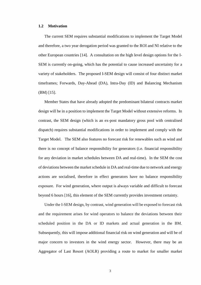
The current SEM requires substantial modifications to implement the Target Model

and therefore, a two year derogation period was granted to the ROI and NI relative to the

other European countries [14]. A consultation on the high level design options for the I-

SEM is currently on-going, which has the potential to cause increased uncertainty for a

variety of stakeholders. The proposed I-SEM design will consist of four distinct market

timeframes; Forwards, Day-Ahead (DA), Intra-Day (ID) and Balancing Mechanism

(BM) [15].

Member States that have already adopted the predominant bilateral contracts market

design will be in a position to implement the Target Model without extensive reforms. In

contrast, the SEM design (which is an ex-post mandatory gross pool with centralised

dispatch) requires substantial modifications in order to implement and comply with the

Target Model. The SEM also features no forecast risk for renewables such as wind and

there is no concept of balance responsibility for generators (i.e. financial responsibility

for any deviation in market schedules between DA and real-time). In the SEM the cost

of deviations between the market schedule in DA and real-time due to network and energy

actions are socialised, therefore in effect generators have no balance responsibility

exposure. For wind generation, where output is always variable and difficult to forecast

beyond 6 hours [16], this element of the SEM currently provides investment certainty.

Under the I-SEM design, by contrast, wind generation will be exposed to forecast risk

and the requirement arises for wind operators to balance the deviations between their

scheduled position in the DA or ID markets and actual generation in the BM.

Subsequently, this will impose additional financial risk on wind generation and will be of

major concern to investors in the wind energy sector. However, there may be an

Aggregator of Last Resort (AOLR) providing a route to market for smaller market

4

participants to manage their imbalances [17]. For instance, empirical evidence from the

Irish wind energy industry suggests the AOLR could provide aggregates of energy output

from multiple wind generators to participate across the different market timeframes and

this could become a precursor to wind not being subsidised through a Renewable Energy

Feed in Tariff (REFIT) or similar policy.

The TSOs will balance supply and demand in the BM timeframe within the I-SEM by

wind curtailment and/or using market participants’ decremental bids in times of surplus

energy or inversely using incremental bids in times of deficit. The cost of procuring

balancing services will be allocated to the imbalanced market participants (i.e. that

deviated from their schedule) and will reflect the marginal costs of energy balancing

actions taken by the TSOs. The increasing amount of wind capacity due for connection

by 2020 and beyond as a result of the Irish government’s electricity targets introduces a

new challenge for the TSOs in maintaining the security and stability of the system. The

use of large scale energy storage such as Pumped Hydro Energy Storage (PHES) and

Compressed Air Energy Storage (CAES) could represent improvements in the AII system

configuration which would reduce the reliance on expensive generation for system

balancing but also reduce the financial risk to wind generation in the I-SEM.

Currently, only one 292 MW PHES plant participates in the SEM and has been

operational since 1974. Furthermore, only one connection agreement has been signed for

a 70 MW PHES plant and there is also a proposal for a sea water PHES plant on the west

coast of Ireland [18]. However, despite PHES being considered a mature technology,

further development in Ireland has ceased mainly due to the lack of suitable sites, high

initial capital costs and environmental impact concerns. Apart from PHES, CAES is the

only commercial large scale energy storage technology to have been deployed at utility

scale and a number of studies have indicated CAES as a solution to improving wind

5

integration and reducing wind curtailment [19]–[21]. A potential CAES site with suitable

geological conditions has been identified in Larne, NI [19], [22]. Hence, the potential

exists for a CAES plant to be connected to the AII system and to participate in the

forthcoming I-SEM [23].

1.3 Aim and Objectives

The aim of this research is to estimate the economic performance of wind generation

with and without CAES, in the I-SEM. Specifically, the system marginal prices, total

generation costs and operational CO2 emissions are estimated under the proposed I-SEM

design in 2020 for various scenarios including with and without CAES. The economic

performances of wind investments under these different scenarios are also assessed.

The specific objectives of this research are to:

collect, verify and analyse technical and financial data from Irish wind energy

projects;

assess the I-SEM from a systems perspective with and without CAES in terms

of system marginal prices, total generation costs and operational CO2

emissions;

evaluate the economic performance of wind generation with respect to balance

responsibility in the I-SEM with and without CAES from a private investor’s

perspective; and

estimate whether investment in CAES is economically viable from a systems

perspective.

6

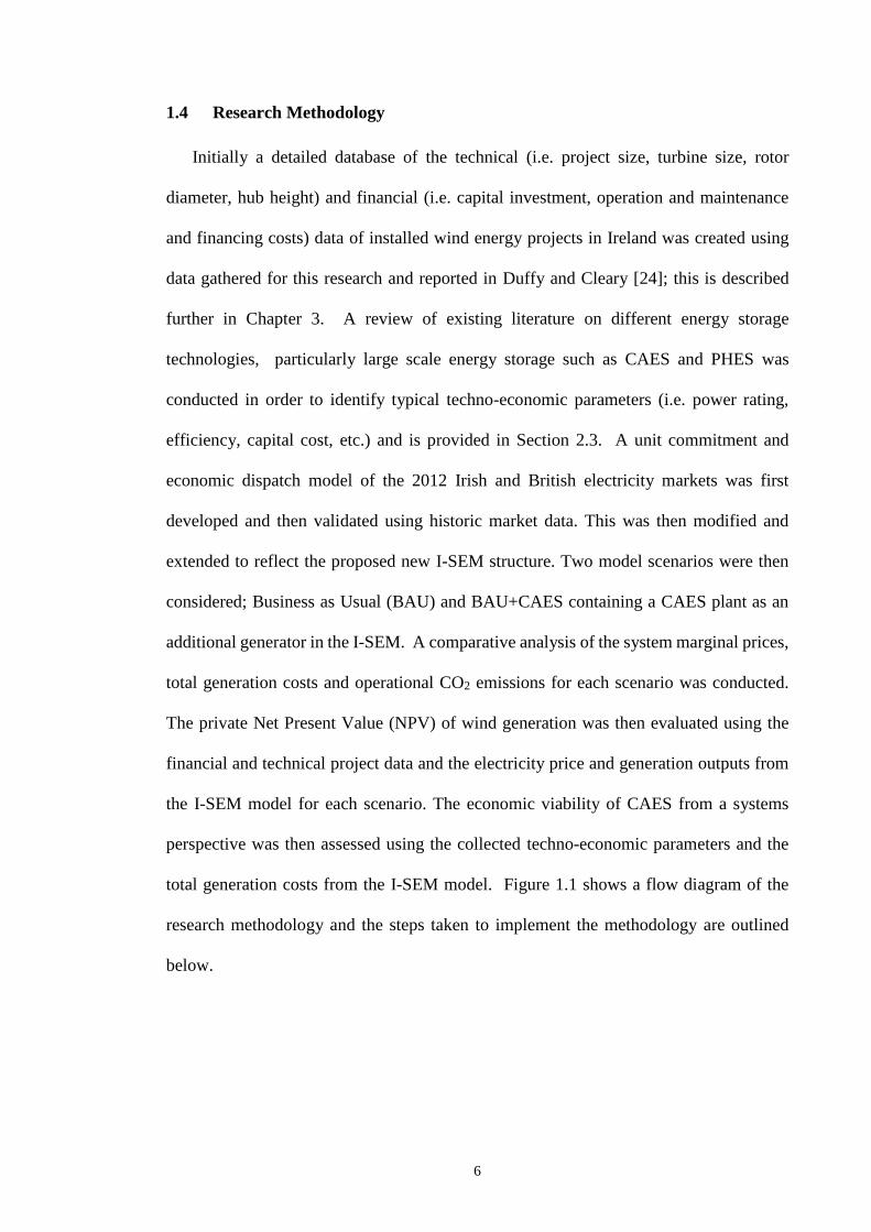
1.4 Research Methodology

Initially a detailed database of the technical (i.e. project size, turbine size, rotor

diameter, hub height) and financial (i.e. capital investment, operation and maintenance

and financing costs) data of installed wind energy projects in Ireland was created using

data gathered for this research and reported in Duffy and Cleary [24]; this is described

further in Chapter 3. A review of existing literature on different energy storage

technologies, particularly large scale energy storage such as CAES and PHES was

conducted in order to identify typical techno-economic parameters (i.e. power rating,

efficiency, capital cost, etc.) and is provided in Section 2.3. A unit commitment and

economic dispatch model of the 2012 Irish and British electricity markets was first

developed and then validated using historic market data. This was then modified and

extended to reflect the proposed new I-SEM structure. Two model scenarios were then

considered; Business as Usual (BAU) and BAU+CAES containing a CAES plant as an

additional generator in the I-SEM. A comparative analysis of the system marginal prices,

total generation costs and operational CO2 emissions for each scenario was conducted.

The private Net Present Value (NPV) of wind generation was then evaluated using the

financial and technical project data and the electricity price and generation outputs from

the I-SEM model for each scenario. The economic viability of CAES from a systems

perspective was then assessed using the collected techno-economic parameters and the

total generation costs from the I-SEM model. Figure 1.1 shows a flow diagram of the

research methodology and the steps taken to implement the methodology are outlined

below.

7

Technical & financial

data gathered for Irish

wind projects

Net Present Value

of wind (€ bn)

Total Generation

Costs (€ bn)

Build 2012 models

CO2 Emissions

(MtCO2)

System Marginal

Prices (€/MWh)

Generation Output

(MWh)

Define model

scenarios

Net Revenue of

CAES (€)

Techno-economic data

gathered for CAES

Step 1

Step 2

Step 3

Step 6

Step 8

Validate 2012 models Step 4

Step 9

Step 7

Build

2020 I-SEM model Step 5

Figure 1.1 Flow diagram of the research methodology

The main steps taken to achieve the research methodology are listed below:

1. Gather and collate detailed technical and financial data for installed wind

energy projects in Ireland.

2. Review existing literature in order to identify the typical techno-economic

parameters of energy storage technologies, particularly CAES.

3. Build detailed 2012 models of the current Irish and British electricity market

structures using PLEXOS.

4. Validate the 2012 model outputs with historic Irish and British electricity

markets data.

8

5. Modify and extend the validated 2012 models to reflect the I-SEM design

and year of study in 2020, respectively.

6. Define and setup the model scenarios BAU and BAU+CAES in the 2020 I-

SEM model.

7. Run the I-SEM model scenarios and determine the system marginal prices,

total generation costs and operational CO2 emissions

8. Estimate the private NPV of wind generation with and without CAES.

9. Estimate the net revenue of CAES from a systems perspective.

1.5 Thesis structure

This section provides an outline of the main topics covered in the succeeding chapters

of this thesis. The thesis comprises seven chapters, commencing with an introduction in

Chapter 1 and ending with conclusions and recommendations in Chapter 7.

Chapter 2 contains a description of the literature in the research area and is split into

five sections. The first section provides an overview of the Global, European and Irish

energy policies and the influence they have on the current and proposed Irish and British

electricity market structures. The global and national evolution of wind power is

described in the second section in terms of the growth of installed wind capacity, growth

of wind turbine sizes and the challenges associated with wind power integration. The third

section provides a brief overview of the different energy storage technologies including

their technological maturity and typical technical and economic characteristics. The next

section presents a high level comparative analysis of the main proprietary modelling

software tools for power systems and market modelling. Lastly, a summary of the

literature review and its implications for the research is presented.

9

Chapter 3 introduces the importance of wind energy costs including trends and drivers

and their relevance to this research. The second section provides details of the

methodology implemented for calculating the Levelised Cost of Energy (LCOE) as well

as the process for collecting and verifying the technical and financial data for Irish wind

energy projects. It also presents the technical and financial data trends for Irish wind

energy projects between 2007 and 2012.

Chapter 4 outlines the methodology implemented for the 2012 base case unit

commitment and economic dispatch model for the SEM and BETTA markets. It consists

of four sections and describes the main model input assumptions and the validation of the

model with historic market data. The chapter introduces the modelling software tool

PLEXOS and provides a brief outline of the approach used to model both SEM and

BETTA markets. It provides a brief description of the model including the main data

sources for the model inputs and the model equations. A detailed description of the model

input assumptions such as the generation portfolio, system demand, interconnectors and

cost input data is also provided. In the final section the base model validation approach

between the base PLEXOS model outputs and the actual SEM and BETTA markets data

is presented.

Chapter 5 outlines the methodology implemented for modifying and extending the

validated base case model to reflect the 2020 I-SEM model. The main model input

assumptions, scenarios and sensitivities are described. The chapter provides a description

of the 2020 I-SEM model including the modifications which were applied to the validated

2012 base model presented in Chapter 4. A detailed description of the model input

assumptions such as the generation portfolio, wind generation, system demand,

interconnectors and cost input data is also provided. The I-SEM model scenarios BAU

and BAU+CAES are described and details of the CAES plant configuration and the

10

modelling approach are outlined. A methodological overview of the economic

assessment of wind generation is also provided. The final section outlines the I-SEM

model sensitivities such as the wind and demand forecast error, generator increments and

decrements, and fuel and carbon prices.

Chapter 6 presents and discusses the main results of the I-SEM model including

system marginal prices, total generation costs and operational CO2 emissions for the

BAU and BAU+CAES scenarios.

Chapter 7 provides final conclusions for the research presented and further

recommendations for future work in the area.

1.6 Research contribution

The contribution to knowledge for research in this area is summarised as follows:

1. Acquisition, analysis and presentation of the first comprehensive technical and

financial data trends analysis of Irish wind energy projects

A review of current literature revealed that very limited up to date technical and

financial data for individual wind energy projects in Ireland currently exists. Therefore,

it is difficult to conduct an accurate economic analysis of wind energy in Ireland.

2. The development and validation of detailed PLEXOS models for the current SEM and

BETTA markets.

PLEXOS has been used by the TSOs, regulators, SEM market participants and

academia for various Irish case studies. Similarly, it has been used for several GB case

studies. Although, a very limited number of these studies validated their PLEXOS model

outputs with historic market data as discussed further in Section 4.4.

11

3. The research represents the first market model simulations of the high-level I-SEM

design under different scenarios and sensitivities.

A review of current literature revealed that no extensive analyses of the I-SEM

design have been conducted and therefore, this prompts further consideration.

Moreover, no I-SEM model development using modelling software tools such as

those described in Section 2.4 have been carried out to date by academia, while the

Irish TSOs have conducted some preliminary I-SEM model simulations which are not

yet publically available. Furthermore, the Single Electricity Market Operator (SEMO)

are coordinated a working group made up of market participants to trial the

EUPHEMIA pricing algorithm for the DA market in the I-SEM.

12

2 LITERATURE REVIEW

2.1 Introduction

This chapter first provides a brief history of global, European and Irish energy

policies. It then describes the current and proposed Irish and British electricity market

structures. The global and national evolution of wind power and wind integration is

described in Sections 2.2 and 2.3. A review of modelling software tools for power

systems and electricity markets is provided in Section 2.4. Finally, a summary is provided

of the current-state-of-the-art as it applies to the research area.

2.1.1 Global energy policy and trends

Global energy use is changing rapidly due to a number of factors including growing

wealth, changing demographics, natural resource depletion, security of supply issues and

environmental concerns. The increased use of unconventional oil and gas and the shift

away from nuclear energy and towards renewable energy for electricity production is

further influencing this change. According to the IEA [25] oil (31%), coal (29%) and

natural gas (21%) are the dominant fossil fuels in the global energy mix as shown in

Figure 2.1. Similarly, in 2012 the share of fossil fuels for global electricity production

was dominated by coal (40.4%) and natural gas (29%) with renewable energy

contributing 5% of total production. Moreover, in the same year, the share of total global

electricity production from fossil fuels in China, the United States (US) and India was

41%, 18% and 9%, respectively [25].

13

Figure 2.1 Share of fuels of global total primary energy (Mtoe) supply in 2012

(*Geothermal, solar, wind, heat; **Peat and oil shale are aggregated with coal)

Globally, China is a key consumer of energy and is currently the world’s largest coal

user, producer and now importer. It has announced plans to reduce the share of coal in

total primary energy demand from 67% to 65% by 2017 and to fast track the introduction

of new vehicle emissions standards [26]. In 2012, China published the 12th Five-Year

Plan (2011-2015) which aims to reduce carbon intensity by 17% by 2015 relative to 2010

levels and raise energy consumption intensity by 16% relative to Gross Domestic Product

(GDP) [27]. Furthermore, China seeks to meet 11.4% of its primary energy requirements

from non-fossil sources by 2015. In 2013, China was the world’s leading renewable

energy producer and had a total installed capacity of 378 GW, mainly from hydropower

and wind power representing 20% and 5% of the total generation capacity mix,

respectively [28].

On the 25th of June 2013 the Obama administration announced the Climate Action

Plan for confronting climate change [29]. It proposes to introduce: (1) new standards

for power plants; (2) additional funding and incentives for energy efficiency and

14

renewable energy; (3) provisions to protect the country from the impacts of climate

change; and (4) steps to provide global leadership to reduce carbon emissions [26].

The so-called shale or unconventional gas revolution, aided by the use of hydraulic

fracturing techniques has emerged as a key aspect of US energy policy. The abundant

supply of shale gas caused energy commodity prices to drop two to threefold in US

markets between 2008 and 2012, creating a range of opportunities, challenges and

unexpected outcomes [30]. In contrast, the US renewables industry continues to be

hampered by inconsistent policy including numerous expirations of the federal renewable

electricity production tax credit (PTC) [31].

In Canada, the government’s Responsible Resource Development (RRD) plan,

introduced in the 2012 budget, has delivered several changes to strengthen responsibility

and ensure a more effective and efficient regulatory system [32]. The RRD plan aims to

enhance Canada’s regulatory system by: (1) making project reviews more predictable and

timely; (2) reducing duplication of these reviews; (3) strengthening environmental

protection; and (4) enhancing Aboriginal consultations [32]. The proposed Keystone XL

pipeline project between Alberta, Canada and Nebraska, US remains high on the US and

Canadian energy policy agenda. The pipeline project will allow Canadian and American

oil producers greater access to the large refineries in the Midwest and Gulf coast of the

US. The pipeline will have a capacity to transport up to 830,000 barrels of oil per day

and will reduce the US dependence on oil from Venezuela and the Middle East by up to

40% [33]. However the project has been hampered by numerous delays as a result of

permitting issues and environmental impact concerns.

India’s energy policy is largely framed around the country’s increasing energy deficit

and the development of alternative energy sources particularly nuclear, wind and solar

power. India has the fifth largest wind power market in the world and proposes to install

15

20 GW of solar power capacity by 2022. It also hopes to increase the share of nuclear

power in the electricity production mix by more than two fold within 25 years and aims

to supply 25% of electricity from it by 2050. Like China, India is highly dependent on

coal and accounts for approximately 55% of commercial energy supply [30]. India also

publishes revolving five year plans, the current 12th Five-Year Plan (2012-2017) sets out

a GDP growth rate of 8% [34].

In 2011, Japan commenced altering its energy policy as a result of the Great East

Japan Earthquake, the Fukushima nuclear plant accident and the subsequent mothballing

of its existing nuclear plants. In May 2013, the Japanese government amended its Act on

the Rational Use of Energy [32]. The Act’s first pillar aims to improve the thermal

insulation performance of houses and buildings with the use of more energy efficient

insulators and windows. It also aims to reduce peak demand by promoting the

introduction of technologies such as smart meters, energy management systems and

energy storage.

Recently, the 196 parties to the United Nations Framework Convention on Climate

Change (UNFCCC) reached an agreement on tackling global climate change on

December 12th 2015 at a conference in Paris. The key outcomes of the conference and

agreement, entitled the 21st session of the UNFCCC Conference of the Parties or COP 21

were [35]:

A long-term goal of limiting the global average temperature increase well below

2oC, while encouraging efforts to limit the increase to 1.5oC;

Establish binding commitments by all parties to make Nationally Determined

Contributions (NDCs) and to pursue domestic measures aimed at achieving them;

16

Commit all countries to report regularly on their emissions and progress made in

implementing and achieving their NDCs, which will undergo international

review;

Commit all countries to submit new NDCs every five years, with a clear

expectation that they will represent progression beyond the previous years;

Reassert the binding obligations of developed countries under the UNFCCC to

support the efforts of developing countries, while for the first time encouraging

voluntary contributions by developing countries too;

Extend the current goal of mobilizing $100 billion a year in support by 2020

through 2025, with a new, higher goal to be set for the period after 2025;

Extend a mechanism to address loss and damage resulting from climate change,

which explicitly will not involve or provide a basis for any liability or

compensation;

Require parties engaging in international emissions trading to avoid double

counting (i.e. where two or more Parties claim the same emission reduction to

comply with their mitigation targets or whereby more than one emission reduction

unit is registered for the same mitigation benefit under different mitigation

mechanisms [36]); and

Call for a new mechanism, similar to the Clean Development Mechanism under

the Kyoto Protocol, enabling emission reductions in one country to be counted

toward another country’s NDC.

While the Paris agreement may be considered aspirational, it requires for the first time

that all parties report regularly on their emissions and implementation efforts which are

internationally reviewed [37]. Furthermore, it will provide a framework that will ensure

that developing countries, like China and India, will alter their energy and climate policy,

17

while developed countries and regions like the US and European Union (EU) will

investigate further decarbonisation of their energy systems. The Paris agreement will be

open for signature on the 22nd of April 2016 and in order to become a party to the

agreement, a country must provide approval to be bound through a formal process of

ratification, acceptance, approval or accession [37].

2.1.2 European Union energy policy

The EU has always played a significant role in alleviating global climate change and

was the driving force behind the Kyoto Protocol implementation in 1997. However, it

was not until 2006 that the basic principles of the EU energy policy were outlined with

the publication of the European Commission’s green paper ‘A European Strategy for

Sustainable, Competitive and Energy’ [38]. The main proposals put forward by the

European strategy were:

a reduction of at least 20% in greenhouse gas (GHG) emissions from all primary

energy sources (electricity, heat, transport, agriculture and built environment) by

2020 relative to 1990 levels, while pursuing an international agreement to succeed

the Kyoto Protocol aimed at achieving a 30% reduction by all developed nations

by 2020;

a reduction of up to 95% in carbon emissions from primary energy sources by

2050, relative to 1990 levels;

a minimum target of 10% for the use of biofuels by 2020;

unbundling of energy supply and generation activities of energy companies from

their distribution networks to further increase market competition;

improving energy relations with the EU's neighbours, including Russia;

the development of a European Strategic Energy Technology Plan to develop

technologies in areas including renewable energy, energy conservation, low-

18

energy buildings, fourth generation nuclear reactor, clean coal and carbon

capture; and

developing an Africa-Europe Energy partnership, to help Africa leap-frog to low-

carbon technologies and to help develop the continent as a sustainable energy

supplier.

While these proposals are considered ambitious, they provided momentum to the EC

and individual EU Member States to create, implement and achieve targets. In 2007, the

most evident was the introduction of the 20/20/20 climate and energy targets, which

defined EU energy and climate change policy in recent years. These targets refer to the

three 20% goals, to be reached by 2020 which involve: a reduction in EU GHG emissions

of at least 20% below 1990 levels, 20% of EU energy consumption to come from RES

and a 20% reduction in primary energy use, to be achieved by improving energy

efficiency [39]. These targets are more ambitious than the targets set out by the Kyoto

protocol and shows that Europe is willing to lead by example when it comes to climate

change mitigation.

A suite of EU directives were enacted in order to ensure the 20/20/20 targets are

achieved. For instance, the Directive 2009/28/EC on renewable energy sets specific

targets for all EU Member States, subject to their renewable potential [1]. The Directive

2002/91/EC on the energy performance of buildings was introduced in 2002 and recast

in 2010 to regulate building standards within EU Member States and focuses on the

delivery of energy efficiency commitments within the building sector. Since its adoption,

member states are required to develop a national framework for the calculation of energy

performances of buildings [40].

A major pillar of the EU’s energy and climate change policy is the European Union

Emissions Trading Scheme (EU-ETS), a cap-and-trade scheme whose members include

19

the largest GHG emitters (circa 11,000 members) in the electrical, industrial and aviation

sectors [41]. For the non-EU-ETS sectors (such as transport, built environment and

agriculture), the EU Effort Sharing Decision (Decision No. 406/2009/EC) establishes

binding annual GHG emissions targets for each Member State’s emissions from each

sector. In 2020, it is envisaged that the emissions from the sectors covered under the EU-

ETS will be 21% lower than in 2005. In the same year, it is envisaged the national targets

will deliver a reduction of around 10 % in total EU emissions from the non-EU-ETS

sectors compared with 2005 levels [42].

The EU-ETS has not performed as expected due to an increasing surplus of

allowances, resulting in the collapse of the carbon price from €30/tCO2 in 2008 to €6/tCO2

in 2014 [43]. The EC has taken the step to postpone (or ‘back-load’) the auctioning of

some of these allowances [44]. The EU-ETS was not designed to be flexible enough to

adapt to the economic crisis depressing growth rates and in turn reducing demand.

Subsequently, the EU-ETS did not attract investment in decarbonisation the power sector

and only had a marginal effect in meeting GHG targets. For instance, in 2012, the

electrical sector remained the largest emitter (circa 38%) relative to the total EU CO2

emissions per sector [43].

In terms of progress towards meeting the 20/20/20 targets, the EU in general is on

track but across each Member State progress varies. The EU reduced emissions between

1990 and 2013 by 19%, therefore it is already close to the target of 20% emissions

reduction by 2020 and seven years ahead of time [45]. Furthermore, aggregated

projections from Member States indicate that total EU-28 emissions will further decrease

between 2013 and 2020. The EU is also on track towards achieving its common target

for renewable energy consumption, with renewables contributing to 14.1% of final energy

consumption in 2012 and higher than the 13% predicted for 2012.

20

Of the EU-28, 22 Member States were on track with their renewable energy

trajectories as defined in their National Renewable Energy Action Plans (NREAPs), while

the remaining 6 underperformed [46]. As regards the interim targets defined in the

Directive 2009/28/EC on renewable energy, 26 Member States met their 2011/2012 goal.

The third EU target on energy efficiency remains a significant challenge, although the EU

is currently on track towards achieving its target mainly due though to the economic crisis

[45]. As economic growth gradually increases across Europe, further efforts will be

required to implement and enforce energy efficiency policies at national level, in order to

ensure that the target is actually met.

Overall, the Member States progress at national level across the three policy target

areas indicate that the EU is making good progress towards meeting its 20/20/20 targets.

However, no EU Member State is on track towards meeting targets across all three policy

areas and 2030 is fast approaching. Therefore, the European Commission is now shifting

its attention beyond 2020 and has been deliberating on a 2030 framework for climate and

energy policies including the extent of any binding targets.

The 2030 framework builds on the experience of, and lessons learnt from, the

20/20/20 targets framework. On the 22nd January 2014, the European Commission

adopted a white paper on energy policy until 2030 at the level of the EU-28.

Subsequently, in February 2014, the European Parliament voted in favour of binding 2030

targets on renewables, emissions and energy efficiency: a 40% cut in GHG emissions,

compared with 1990 levels; at least 30% of energy to come from renewable sources; and

a 40% improvement in energy efficiency, respectively. As of October 2014, the EU

leaders agreed on a 40% cut in GHG emissions relative to 1990 levels, at least 27% of

energy to come from renewable sources and a 27% improvement in energy efficiency

[47].

21

2.1.3 Irish energy policy

EU energy policy heavily influences each Member State’s energy policy including

Ireland’s which is framed within the 20/20/20 targets. Ireland’s NREAP, which is

consistent with the EU Directive 2009/28/EC on renewable energy, was published in

2009 [5]. Under the NREAP, Ireland’s overall target is to ensure at least 16% of gross

final energy consumption is produced from renewable sources by 2020 (compared with

3.1% in 2005). The overall mandatory target consists of a 40% of electricity consumption

from renewable sources (RES-E), 12% renewable heat (RES-H) and 10% renewable

transport (RES-T). The majority of the RES-E share (circa 37%) will be met from land-

based wind energy, given the significant wind resource which exists in Ireland and the

maturity of the technology nationally. Similarly in Northern Ireland, the Department of

Enterprise, Trade and Investment published the Strategic Energy Framework in

September 2010 which sets out a 40% RES-E share by 2020 [48]. In 2013, Ireland was

on average, half way towards meeting its 2020 targets, having achieved 21% of electricity

generation, 4.9% of transportation and 5.7% of heat production from RES [49]. Ireland

is likely to achieve the RES-E share of the 2020 target, however rapid growth in the RES-

H and –C shares needs to accelerate if the 2020 target is to be achieved.

The development of renewable energy is central to energy policy in Ireland and the

majority of the RES-E target (circa 37%) will be met from onshore wind energy given

the significant wind resource which exists in Ireland. The Renewable Energy Feed-In

Tariff (REFIT) scheme was introduced to help meet the RES-E target and thus provided

a relatively stable investment environment. As a result of such schemes, in 2013, Ireland

produced approximately 18% of its electricity demand from wind, with an installed

capacity of 1,999 MW [49]. A total installed onshore wind capacity of 3,575 MW is

planned for 2020 to meet policy targets, requiring the addition of 1,576 MW in the period

22

2014-2020 [7]. Also, after several years of debate, a carbon tax was implemented in 2010

to help decarbonise the Irish economy, which applies to much of the economy that is not

covered by the EU-ETS [50].

The 2007 Irish government energy policy white paper, ‘Delivering a Sustainable

Energy Future for Ireland’ set out three main pillars of Irish energy policy:

competitiveness, energy security, and sustainability [51]. Since its publication, it has

provided policy certainty and a wide range of detailed action plans, schemes, measures

and investment programmes up to 2020 as outlined above. As the European Commission

now shifts its attention towards 2030 and 2050, the Department of Communications,

Energy and Natural Resources (DCENR) published a green paper on energy policy in

May 2014, which invites written views, observations and suggestions from stakeholders

on the future of Ireland’s energy policy [52]. On completion of the consultation process,

a new energy policy white paper will be developed which sets out an energy policy

framework for the medium and long terms. Furthermore, more recently, the Irish State’s

first ‘Climate Action and Low Carbon Development Bill 2015’ was published in January

2015 and sets out a more generalised approach to enabling the transition towards a low

carbon economy by 2050 [53]. However, there is no explicit targets contained in the Bill

but it formally obliges the Irish State to adhere to EU targets or global agreements.

2.1.4 Ireland’s electricity market

Electricity plays an important role within the Irish energy mix and the SEM, which

forms the backbone of the AII power system, is poised to play an increasingly strategic

role in achieving Ireland’s energy policy ambitions. The SEM is the current AII wholesale

electricity market covering the ROI and NI, which has been operational since November

2007 [9], [10]. However, the current market arrangements are subject to change by 2018

23

due to EU legislation designed to harmonise cross border trading arrangements across all

European electricity markets [11].

The SEM is an ex-post mandatory pool market operating on a bid-based exchange with

dual currencies and in multiple jurisdictions. Electricity is bought and sold from the pool

through a market clearing mechanism by which generators bid in their offers and, where

they are dispatched, receive the System Marginal Price (SMP) for each trading period as

shown in Figure 2.2 [54].

Figure 2.2 SEM overview (Source: [55])

Generator offers consist of commercial offer data (.i.e. fuel cost, no-load cost and

start-up cost) and technical offer data (.i.e. max capacity, min stable level and ramp rates).

The SMP consists of two components known as the “shadow” and “uplift’’ prices. The

shadow price makes up most of the SMP and relates to the incremental short run marginal

cost (SRMC) bids from generators comprising mainly of fuel costs. The uplift price is a

payment put in place to avoid generators making short term losses and covers the

generator’s start-up and no-load costs [10]. Any generator whose SRMC is at or below

the cost of the marginal generator which meets the last unit of demand is instructed at this

time if it will be dispatched and the quantity of generation required for dispatch. If it is

24

“out of merit”, i.e. if it is SRMC is above the cost of the marginal generator it will know

at this time that it will not be dispatched as shown in Figure 2.3 [10].

Figure 2.3 Indicative SEM schedule (Source: [56])

Generators participating in the SEM receive payments for energy via the SMP but

they also receive a capacity payment for making their capacity available which

contributes towards their fixed costs and ensures security of the system. There are also a

number of other payments to generators in the SEM including uninstructed imbalances

and constraint payments. In particular, alterations to the scheduled dispatch which

inevitably occur in the real time system operation result in the issue of constraint

payments to ensure the generators stay financially neutral due to the difference between

the market and actual dispatch schedules. In 2014, the energy, capacity and constraints

costs made up 74% (70% “shadow” and 30% “uplift” costs) , 20% and 6% of the annual

SEM wholesale costs, respectively [9]. The electricity price which the Irish consumer

pays is generally made up of wholesale costs (circa 60%), network costs (circa 30%) and

supplier costs (circa 10%) [56].

25

According to Gorecki [57] ‘the SEM has been successful in meeting the challenges of

mitigating market power, facilitating entry and ensuring adequate generation capacity’.

However, one aspect of the SEM which has not worked efficiently is the trading of

electricity across the interconnectors between the SEM and BETTA markets [57], [58].

An analysis by McInerney et al. [58] indicates significant power flows against the

efficient price spread direction (i.e. at times the flows go from the high price to the low

price jurisdiction) which implies higher costs than necessary for consumers in Ireland

and/or in GB. The main reasons cited for the inefficiencies include ex-post pricing in the

SEM (i.e. the final ex-post SMP is not published until four days after the trading day),

intermittent wind and strategic behaviour by dominant firms [58]. For instance, if high

levels of wind generation are forecasted in the ex-ante SMP run in combination with the

final interconnector power flows and less wind generation is dispatched in real time. This

will affect the final ex-post SMP run and the optimal price spread direction as the GB

price remains fixed while the SMP is subject to change.

The SEM is currently being redesigned to achieve compliance with the European

Target Model and ensure more efficient use of the interconnectors, which should provide

increased access to lower cost generation, and facilitate increased exports [59]. The main

challenge is integrating the redesigned SEM with the adjacent electricity markets and it

will require substantial modifications to implement the Target Model, thus a two year

derogation period was granted to Ireland relative to the other European countries.

In September 2014, the regulators published the high level design for the I-SEM and

a consultation process on the detailed design is currently on-going [17]. The I-SEM

design will consist of four distinct markets: Forwards, DA, ID and BM as shown in Figure

2.4. In the Forwards market only financial trading instruments are permitted for forward

trading. For instance, power traded across the Irish interconnectors to Britain will be

26

traded using Financial Transmission Rights (FTRs) as opposed to Physical Transmission

Rights (PTRs), which operate on most of the interconnectors in Europe. The FTRs could

be structured as options or obligations and may take the form of a Contract for Difference

(CfD) against a DA reference price.

Figure 2.4 Proposed high level design for I-SEM

The DA market will be the exclusive route to a physical contract nomination within

the DA time frame. Participants will be required to submit hourly price-quantity bids in

advance of gate closure (11:00am) for the trading day starting at 11:00pm Greenwich

Mean Time (GMT) [17]. Participation for generation will generally be on a unit-basis

with aggregation for demand (i.e. demand side units) and some variable renewable

generation. The ID market will involve continuous intraday trading and will be the

exclusive route to physical contract nominations (with scope to introduce periodic

implicit auctions if these develop at the European level). The ID market will open after

27

the DA market results have been published with trading expected to be on an hourly basis

until one hour prior to the delivery hour [17].

Mandatory participation in the BM will be required after the DA market and

participants will be required to submit incremental and decremental bids so they can be

moved from their nominated position if required. Participation in the BM will be on a unit

basis and there will be marginal pricing for unconstrained energy balancing actions (i.e.

to balance supply and demand) and ‘pay as bid’ for non-energy actions (i.e. to ensure all

system constraints are respected in order to maintain a secure power system) [17]. The

imbalances between metered generation and nominated position will be settled on a unit

basis based on a single imbalance price. It is envisaged that the imbalance price will be

based on the cost of the marginal energy balancing action.

As stated earlier, participants in the SEM receive a capacity payment for making their

capacity available which contributes towards their fixed costs. The capacity payments

are paid on a monthly basis from a predetermined annual capacity payment ”pot”, which

is calculated by the CER based on the capital costs and required quantity of generation.

The capital costs and quantity of generation are based on the cost of the ‘Best New

Entrant’ and the expected annual peak demand as forecast by the TSOs, respectively [60].

In 2014, the capacity requirement and annual capacity payment sum was 7,049 MW and

€565,819,301, respectively [60]. At present, capacity is paid for by dividing the capacity

payment “pot” among all available generators. Gas generators are the largest recipient of

capacity payments based on their high levels of availability and the large volume of gas

generation in the SEM [56].

Under the I-SEM design, the current SEM’s capacity payment mechanism will be

replaced by a quantity-based Capacity Remuneration Mechanism (CRM) based on

reliability options [17]. In accordance with the CRM, the capacity requirement will be

28

determined according to a defined adequacy standard set by the regulators (the CER). The

capacity requirement for a given period will be procured through a competitive auction

by a central buyer (most likely the TSO) in advance of the period. The generators

participate in the competitive auction in order to hold reliability options in a given year.

The total amount of options sold in the auction will be equal to the estimated maximum

level of electricity demand for the year at a pre-announced strike price [61], [62]. The

strike price will be determined during the detailed design of the I-SEM by the regulators

and announced in advance of the auction [17].

Generators which hold reliability options can be called upon by the TSO to generate

at periods of system stress. These are identified as periods when the wholesale market

prices (e.g. spot price) rise above a strike price [62]. For instance, where the market price

is greater than the strike price, generators holding reliability options pay the difference

between the market price and strike price back to the TSO and where the market price is

less than the strike price, there is no payment from the generator to the TSO. This

difference payment incentivises generators (i.e. the capacity providers) to be available

during periods of high prices and protects the consumers from price spikes above the

strike price. Reliability options have been implemented in the Columbian and New

England, USA electricity markets and are currently being implemented in the Italian

market [61].

An early study on the implications of the European Target model for Ireland by

Gorecki [63] evaluates and identifies the important issues which need to be addressed

through further research. It concludes that the creation of the EU internal market should

benefit Ireland in terms of lower electricity prices, a more competitive market and greater

security of supply. However, there are three important caveats; first, it assumes no major

policy failure in UK energy policy that results in an unanticipated increase in electricity

29

prices that cannot be offset by increasing interconnection between GB and continental

Europe. Second, it assumes that in complying with the EU’s Third Energy Package, that

Ireland will be given sufficient flexibility in order to avoid potentially costly changes to

the SEM. Thirdly, it assumes that the internal market and interconnection do not become

used as a reason for exporting subsidised renewable energy, leading to higher prices

through increased Transmission Use of System (TUoS) and Public Service Obligation

(PSO) charges.

Based on Gorecki’s [63] caveats, the forthcoming referendum on the UK withdrawal

from the EU referred to as Brexit may result in UK energy policy uncertainty. If the UK

were permitted to participate in the EU following a Brexit, it is envisaged they will need

to negotiate an appropriate partnership with the EU and adopt and comply with the

relevant European legislation such as the EU’s Third Energy Package. The difference,

however, would be that the UK is unlikely to have a say in the formulation and

interpretation of the rules, unless they manage to negotiate to remain part of the

institutions which co-ordinate EU energy regulation such as ACER and ENTSO-E [64].

If the UK fails to do so, it may result in divergence of the UK and EU energy regulatory

regimes.

A more recent study by Gorecki [57] states that ‘aligning the SEM with the European

Target model appears very much to be a matter of fitting a square peg into a round hole’

given the ex-post gross mandatory pool SEM design in comparison to the bilateral

contracts market design under the Target model. The solution to this is changing the

shape of the peg (i.e. the redesign of the SEM) but Gorecki [57] suggests this is not a

sensible choice. Instead, some kind of device needs to be implemented which permits the

peg to fit into the hole in the form of CfDs which act as a mediating device between the

SEM and the rest of the EU internal electricity market [57].

30

Di Cosmo et al. [61] also examined the redesign of the SEM and in particular the high

level of supplier concentration which exists in the market. They cite that the I-SEM

design raises concerns regarding ‘the potential to realise competitive outcomes in the

spot, retail and capacity markets’. Furthermore, they suggest that due to the lack of

competition in the deregulated retail market; vertically integrated firms will potentially

exploit market power and the new CRM will also be vulnerable to the exploitation of

market power in the auction of the reliability options [61]. Therefore, they recommend

that the dominant firms face regulation of the prices and quantities they bid into the new

CRM [61], [62]. Finally, Di Cosmo et al. [61] states that ‘spot market prices and retail

prices should be closely monitored and retail margins should be made publicly available’

in order to ensure a competitive outcome for consumers.

As well as introducing different energy trading timeframes to the SEM through the I-

SEM design, there is also a significant on-going redesign of the current ancillary services

(or system services) mechanism. The ancillary services mechanism is operated outside

of the SEM by the TSO which compensates generators from a “pot” of up to

approximately €60 million for the provision of three services: black start, reactive power

and operating reserve [65]. The number of services and the payment structures for these

services is currently under review by the TSOs, which are in consultation with market

stakeholders under the Delivering a Secure Sustainable Electricity System (DS3)

programme of work [6], [66]. The DS3 programme is a large project which includes

eleven work streams; two of the most important of these are Rate of Change of Frequency

(RoCoF) and System Services, requiring significant stakeholder and regulatory input. If

fully implemented the DS3 programme will deliver significant changes to the operation

of the SEM, not least the facilitation of a SNSP limit of renewable electricity of up to

75%. Moreover, the SEM’s 37% of Variable Non-Synchronous Renewable (VNSR)

31

generation of electricity demand in 2020 is far greater than the three main synchronous

systems with proposed VNSR penetration levels of 22% in GB, 18% in Continental

Europe and 8% in Scandinavia [6].

The TSOs plan to expand the number of services to include: Synchronous Inertial

Response, Fast Frequency Response, Dynamic Reactive Response, Ramping (1, 3 and 8

hour) and Fast Post Fault Active Power Recovery as shown in Table 2.1.

System Services Products Product type Status

Synchronous Inertial Response (SIR) Frequency Proposed

Fast Frequency Response (FFR) Frequency Proposed

Fast Post-Fault Active Power Recovery

(FPFAPR) Frequency Proposed

Ramping margin (RM1,RM3,RM8) Frequency Proposed

Operating reserve (POR,SOR,TOR1,TOR2)2 Frequency Existing

Replacement Reserve (RR) Frequency Existing

Dynamic Reactive Response (DRR) Voltage Proposed

Steady State Reactive Power (SRP) Voltage Existing

Blackstart

System

restoration Existing

Table 2.1 Existing and proposed system services (Source: [67])

In order to incentivise electricity generators to provide additional services, the TSO

attributes costs to these additional services, based on the cost that curtailment imposes on

the system (i.e. when variable renewable generation such as wind is curtailed it is

necessary for other generators to be brought onto the system at short notice) and the cost

foregone when renewable generation, which has a marginal cost of zero, is replaced on

the system by another fuel source.

The SEM Committee (SEMC) at present approves of the policy, rates and overall

monies for the new ancillary services and has decided that an annual expenditure cap

(i.e. the cap limits expenditure to a maximum level but does not guarantee that this level

2Primary Operating Reserve (POR), Secondary Operating Reserve (SOR) and two classes of Tertiary

Operating Reserve (TOR1 and TOR2)

32

of monies will be spent) of €235 million will apply in 2020 [68]. The purpose of setting

an expenditure cap is to limit the exposure of consumers to costs associated with system

services. In the intervening years, the annual cap will increase incrementally from its

current level (€60 million per annum) in line with the delivered volume of system services

and increased SNSP [68]. The modelling work conducted by the TSO indicates that by

2020 the benefit to consumers will be €177 million per annum, which is essentially the

benefit to consumers of moving from a 50% to 75% SNSP limit by 2020 so more low

cost variable renewable generation can be accommodated by the AII system. The SEMC

[68] suggested that the current €60 million system service expenditure is added to the

€177 million additional benefit from further expansion of the SNSP limit. This would

equate to an expenditure cap of €237 million but the SEMC has rounded down to €235

million per annum. The SEMC [68] state that ‘a glide path (with an annual expenditure

cap) to the cap of €235m in 2020 will be established in the detailed design and

implementation phase’. This will be based upon the required volumes of system services

for each of the years 2016 – 2020, which will be developed by the TSO following public

consultation and aligned to deliver a 75% SNSP limit [68].

The SEMC [68] considers that the relative value of the revenue streams coming from

energy, system services and capacity payments will change, but the total revenues should

not alter significantly as shown indicatively in Figure 2.5.

33

Figure 2.5 Indicative rebalancing of revenue streams from SEM to I-SEM

(adapted from [68])

Accordingly the SEMC has designed the system services procurement mechanism to

interact with the energy trading arrangements and CRM in the I-SEM in order to provide

appropriate economic signals for generators to provide increased value to the end

consumer [68]. For instance, as the level of zero marginal cost generation such as wind

on the system increases, this should result in a lower level of revenue in the energy

payments portion as shown in Figure 2.5 for the I-SEM. However, in order to deliver

this low marginal cost generation, a higher portion of revenues will need to be allocated

to system services provision. This will mean that system services will now become an

important aspect of a generator’s revenue streams in order to recover their capital costs.

34

Therefore, lower variable costs and higher fixed costs may result in lower energy

payments but higher system service payments, which should also lower capacity

payments [68].

A major expansion of the AII transmission network is also required between now and

2020 in order to meet Ireland’s RES-E targets and to ensure the secure and efficient

operation of the AII power system and electricity market. In recognition of these

requirements, the TSOs published a €3.2 billion transmission network capital investment

plan up to 2025 entitled Grid25 [6]. In 2011, the scale of the Grid25 strategy was revised

from €4 billion to €3.2 billion to adjust for the downturn in the economy. The Grid25

project includes the building of approximately 1,150 km of new high voltage power lines

and the upgrading of 2,300 km of existing lines, which will double the size of today’s

electricity transmission grid [6]. An independent study by Indecon suggests the

expenditure programme for Grid25 will directly and indirectly support 2,896 jobs on

average for 15 years [69]. More recently, the TSOs published a consultation paper on

Ireland’s grid development [70]. The paper states ‘Ireland’s energy transmission needs

can be met with reduced new infrastructure build because of new technological

developments and updated projections of future electricity demand’. Subsequently,

subject to public consultation and a review of future energy needs and technological

possibilities, the total cost of Grid25 will be revised down from €4 billion in 2008 to

between €2.7 billion and €3.9 billion.

2.1.5 Great Britain’s electricity market

The Great Britain (GB) electricity market, abbreviated as BETTA has been

operational since April 2005 as an energy only market which does not offer any form of

capacity payments [71]. The arrangements under BETTA are based on bilateral trading

between generators, suppliers, traders and customers across a series of markets operating

35

on a rolling half-hourly basis. Under these arrangements generators self-dispatch rather

than being centrally dispatched by National Grid Plc., the TSO. There are four stages to

the BETTA market: forwards/futures contract market, short-term bilateral market (Power

Exchanges), balancing mechanism and imbalance settlement as shown in Figure 2.6. The

contract and bilateral markets typically account for 98% of total traded volumes with the

remaining 2% taking place through the balancing mechanism [72].

Figure 2.6 BETTA market structure (Source:[73])

The forwards/futures contract market allows trading typically up to a year or more

ahead of real time but trading up to gate closure (1 hour before real time) is also possible

[74]. Trading within this market largely comprises of confidential commercial bilateral

transactions and consequently, prices and volumes traded are not publicly available. The

short-term bilateral market operates under similar conditions but trading tends to take

place 24 hours prior to gate closure [74]. This enables generators and suppliers to adjust

their rolling half hour trade contract positions as their own demand and supply forecasts

become more accurate as real time approaches. Trading within the forwards and short-

36

term markets can take place on exchanges, Over the Counter (OTC) (by phone or directly

via the broker trading screens) and bilaterally between two counter parties.

There is also an opportunity for generators and suppliers to participate in the balancing

mechanism. The balancing mechanism operates from gate closure through to real time

delivery and is managed by the TSO. This involves generators and suppliers submitting

offers and bids to alter their generation and demand, respectively, one hour prior to real

time delivery, which helps to balance the system [74]. Finally, the imbalance settlement

is used to settle discrepancies between the amount of electricity which a market

participant contracted to generate or consume and the metered volumes of electricity

which they actually generated or consumed. There are two cash-out prices known as

‘Energy Imbalance Prices’ which are calculated each half hour. They are the ‘System Buy

Price’ (SBP) and the ‘System Sell Price’ (SSP). The SSP is paid to those with a net surplus

of imbalance energy and SBP is paid by those with a net deficit [74].

A consultation on the redesign of the BETTA market structure is currently on-going.

The UK government’s Electricity Market Reform (EMR) programme is designed to

modify the BETTA market instead of replacing it with a new market [75]. Pursuant to

the Energy Act 2013 [76] , the EMR programme aims to provide two key mechanisms:

Contract for Differences (CfDs), and capacity payments, in order to incentivise

investment in low carbon technologies and ensure security of supply, respectively [77].

The CfDs will support low-carbon technologies by providing eligible generators

increased price certainty through a long-term contract. The capacity payments will

provide investors with the certainty they require to put adequate reliable capacity in place.

Another market reform which is currently on-going is the introduction of a single

marginal cash-out price instead of the existing dual cash-out prices for the imbalance

37

settlement process [78]. This cash-out price mechanism will align with the European

Target Model and also the proposed I-SEM design.

2.2 Wind power

This research is primarily concerned with the techno-economic modelling of wind

power integration and large scale energy storage on the Irish power system. The following

subsections therefore provide an overview of the global and national evolution of wind

power in terms installed wind capacity, growth of wind turbine sizes and the associated

challenges with wind power integration. In particular, subsection 2.2.2 outlines the key

enabling technologies (i.e. large scale energy storage) for wind power integration and

reviews a number of interrelated studies on the Irish power system.

2.2.1 Evolution of wind power

Wind power is a mature technology long exploited by humans. For thousands of years

wind was used to provide propulsion for boats along the Nile River and it was harnessed

by the Persians to pump water and grind grain between 500 and 900 B.C [79]. The use

of windmills spread from Persia to the surrounding areas in the Middle East, where they

were mainly used for food production and processing. Around 1,000 A.D., wind power

technology spread to northern European countries such as the Netherlands, which adapted

windmills to help drain lakes and marshes in the Rhine River Delta. However, with the

emergence of cheap fossil fuels and rural electrification in the late 19th and 20th centuries,

the use of wind power declined. During the 20th century and partially due to the onset

of World Wars I and II (i.e. small wind generators were used on U-boats to recharge

batteries) interest in wind power in Europe began to emerge [80]. However, despite some

technological advances during the 1950s and 1960s, interest and research in wind turbines

38

and the power they generated did not advance until the price of oil rose dramatically in

1973. This caused a renewed interest in wind technology for electricity production.

Since 1980, wind power has gained remarkable popularity worldwide as countries

strive to increase the production of renewable energy in order to meet future energy

demand, mitigate global warming and achieve binding policy targets. The global

cumulative installed wind capacity at the end of 2014 was 369.6 GW as shown in Figure

2.7, with an average annual growth rate of almost 23% over the last decade (2005-2014)

[2].

Figure 2.7 Global cumulative installed wind capacity 1997-2014 (Source: [2])

A record year in 2014 was achieved by the wind industry as annual global installations

exceeded 51 GW, a sharp increase in comparison to 2013, when just over 35.6 GW was

installed [2]. The previous record was set in 2012 when over 45 GW of new capacity

was installed globally. Wind power has become the least-cost option for new renewable

power generating capacity in an increasing number of locations, and new markets

continue to emerge in Africa, Asia, and Latin America [2]. Asia remains the largest

market for the seventh consecutive year, led by China, and has overtaken Europe in total

installed capacity. In 2014 total investments in the clean energy sector reached a high of

0

50

100

150

200

250

300

350

400

1997

1998

1999

2000

2001

2002

2003

2004

2005

2006

2007

2008

2009

2010

2011

2012

2013

2014

Cap

aci

ty (

GW

)

Year

39

€277 billion [2]. The global wind sector experienced an investments rise of 11% to a

record €88.9 billion during that year. This was a significant growth in comparison to 2013

investment of €71.7 billion and €72.3 billion in 2012.

Recent global capital investment costs for wind projects reached a peak around 2010

and have declined in most countries since then despite the increase in wind turbine sizes

[81]. This trend is most evident in Denmark and the United States. However, Germany,

Ireland and Norway do not demonstrate this decline, although it may be realised in the

near term [81]. The country specific cost of wind of energy in Ireland is outlined and

discussed in more detail in Chapter 3.

In 2014, 12.9 GW of wind power was installed across Europe, with the EU-28

Member States accounting for 11.8 GW of the total. Moreover, the EU-28 installed more

new wind capacity than gas (2.3GW) and coal (3.3GW) combined in 2014 [82]. In 2014,

there was almost 128.8 GW of installed wind capacity in the EU-28 with a total

cumulative capacity of 134 GW for all of Europe. The cumulative market growth rate in

2014 was 10.5%, although the annual market growth rate was only 4.2% in the EU-28,

and 5.1% in Europe as a whole [82]. At the end of 2014, wind power provided

approximately 10.2% of the EU’s electricity needs. Wind met 8% of the EU’s electricity

demand by the end of 2013, up from 7% at the end of 2012, 6.3% at the end of 2011 and

4.8% at the end of 2009 [82].

For Ireland, the cumulative and annual installed wind capacity for each year since

2000 is shown in Figure 2.9. Prior to 2000, the majority of electricity demand in Ireland

was met by traditional forms of generation such as gas, coal and oil. The installed wind

capacity increased almost four-fold between 2000 and 2005, from 114 MW to 506 MW.

This included the first offshore wind plant with an installed capacity of 25 MW in 2003.

However, the rate of capacity growth fluctuated throughout the period 2000–2013 for a

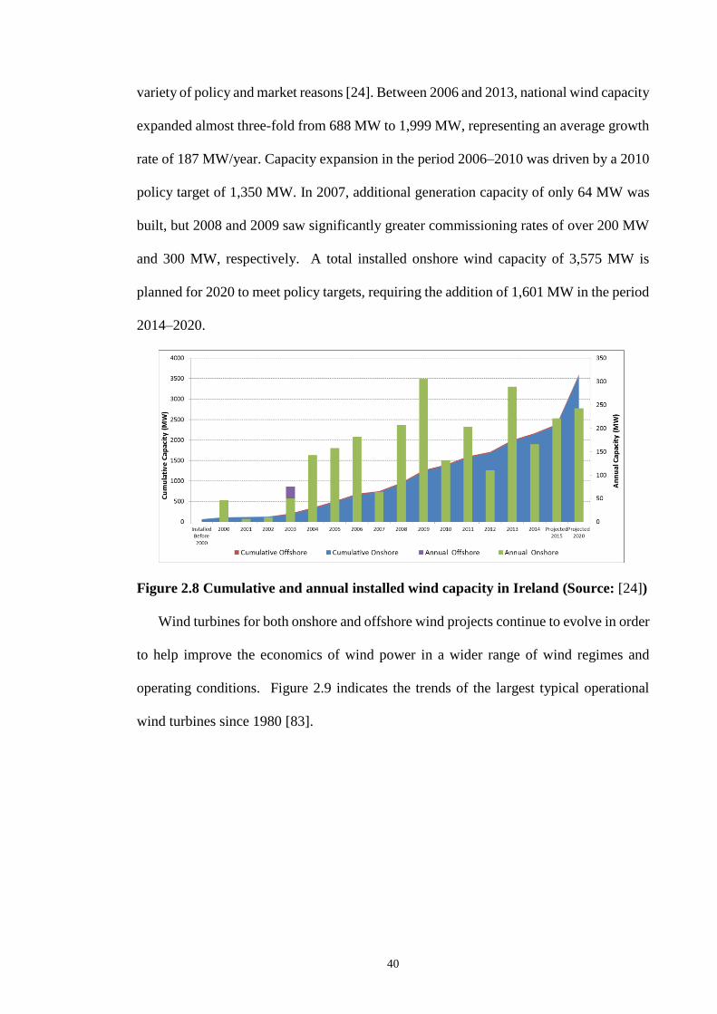
40

variety of policy and market reasons [24]. Between 2006 and 2013, national wind capacity

expanded almost three-fold from 688 MW to 1,999 MW, representing an average growth

rate of 187 MW/year. Capacity expansion in the period 2006–2010 was driven by a 2010

policy target of 1,350 MW. In 2007, additional generation capacity of only 64 MW was

built, but 2008 and 2009 saw significantly greater commissioning rates of over 200 MW

and 300 MW, respectively. A total installed onshore wind capacity of 3,575 MW is

planned for 2020 to meet policy targets, requiring the addition of 1,601 MW in the period

2014–2020.

Figure 2.8 Cumulative and annual installed wind capacity in Ireland (Source: [24])

Wind turbines for both onshore and offshore wind projects continue to evolve in order

to help improve the economics of wind power in a wider range of wind regimes and

operating conditions. Figure 2.9 indicates the trends of the largest typical operational

wind turbines since 1980 [83].

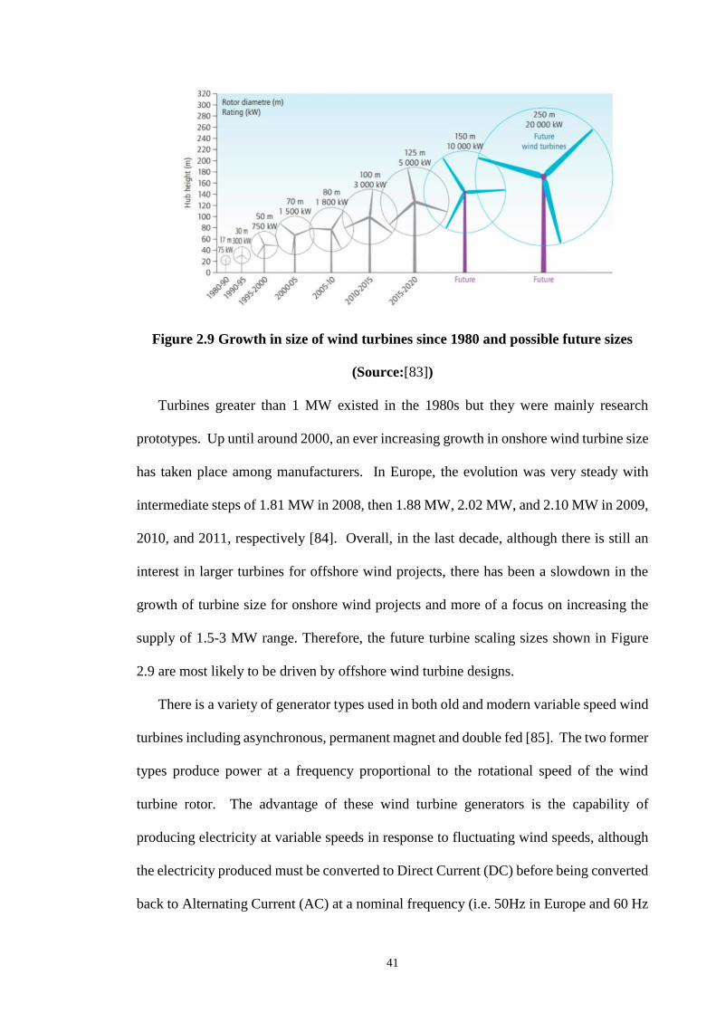
41

Figure 2.9 Growth in size of wind turbines since 1980 and possible future sizes

(Source:[83])

Turbines greater than 1 MW existed in the 1980s but they were mainly research

prototypes. Up until around 2000, an ever increasing growth in onshore wind turbine size

has taken place among manufacturers. In Europe, the evolution was very steady with

intermediate steps of 1.81 MW in 2008, then 1.88 MW, 2.02 MW, and 2.10 MW in 2009,

2010, and 2011, respectively [84]. Overall, in the last decade, although there is still an

interest in larger turbines for offshore wind projects, there has been a slowdown in the

growth of turbine size for onshore wind projects and more of a focus on increasing the

supply of 1.5-3 MW range. Therefore, the future turbine scaling sizes shown in Figure

2.9 are most likely to be driven by offshore wind turbine designs.

There is a variety of generator types used in both old and modern variable speed wind

turbines including asynchronous, permanent magnet and double fed [85]. The two former

types produce power at a frequency proportional to the rotational speed of the wind

turbine rotor. The advantage of these wind turbine generators is the capability of

producing electricity at variable speeds in response to fluctuating wind speeds, although

the electricity produced must be converted to Direct Current (DC) before being converted

back to Alternating Current (AC) at a nominal frequency (i.e. 50Hz in Europe and 60 Hz

42

in North America) thereby incurring energy losses [86]. Conventional fossil fuel-based

generators use so-called synchronous generators to produce electricity and are connected

to the power system via a direct, electro-mechanical link and have a considerable amount

of spinning mass (inertia) [87]. Wind turbines are generally linked to the power system

more indirectly via power electronics and have less or no spinning mass (inertia) and are

non-synchronous generation technologies.

The most common variable speed wind turbines connected to power systems

worldwide use with either asynchronous or permanent magnet generators which do not

contribute to power system reserves and total system inertia. However, wind turbines

with double fed generators do provide synchronous inertia to the power system, and

therefore have the ability to counteract increases or decreases in system frequency in a

similar way to conventional fossil fuel-based generators [85]. The use of double fed

generators is expected to become more common in the coming years as grid codes become

more demanding in order to cope with of the instantaneous penetration level of wind

power increasing in regional power systems [88]. Increasing amounts of installed wind

capacity have therefore meant that, at times of high wind output, the system inertia has

dropped resulting in systems where the frequency can fluctuate faster than normal. This

can create problems for the TSOs and has led some systems such as Ireland to limit the

proportion of electricity that wind is permitted to contribute to its system [89]. Wind

turbine suppliers have acknowledged the lack of inertia response provided by the

generators and the impact this could have on the long-term growth of the wind industry,

hence they are actively pursuing a variety of solutions to counteract this issue [90]. The

following section discusses the challenges of wind power integration and the potential

enabling solutions.

43

2.2.2 Challenges of wind power integration

Traditionally, most power systems and markets were designed to deal with variability

of supply and demand on different timescales, primarily using controllable conventional

synchronous generators. However, nowadays power systems and their associated

electricity markets are under additional pressure due to the integration of RES, in

particular non-synchronous sources such as wind, which has variable operational

characteristics.

A report by Sims et al. [86] states that as variable wind penetration levels increase,

maintaining system reliability becomes more challenging and costly. As power systems

and electricity markets are considerably different worldwide, there is no one set of

guidelines to apply to the problem of RES integration. Consequently, depending on the

specifics of a given power system and electricity market, a portfolio of solutions to

minimise the risks to the system and the costs of RES integration can include the

development of flexible generation, strengthening and extending the network

infrastructure, interconnection, energy storage technologies and modified institutional

arrangements including regulatory and market mechanisms [86].

According to Nikolakakis et al. [91] the rapid growth of solar and wind power has

challenged power systems and the impact of variable RES integration and its associated

costs can be reduced by a set of complementary solutions. These solutions include adding

flexible generation, combining resources such as solar and wind to reduce variability,

using smart grids and storing electricity. In Foley et al. [92] the focus is solely based on

the role and relevance of energy storage and smart grid technologies to integrate the next

generation of renewable power systems. However, they highlight that the weakest links

in terms of delivering a RES future using such technologies is the lack of international

44

standards, real competitive market environments as well as government and regulatory

policies [92].

A study by the IEA [87] investigated the technical flexibility options including grid

infrastructure, dispatchable generation, storage and demand-side management for

Variable Renewable Energy (VRE) integration based on seven case studies in 15

countries; Brazil, Electric Reliability Council of Texas (Texas, United States), Iberia

(Portugal and Spain), India, Italy, Japan East (Hokkaido, Tohoku and Tokyo) and North

West Europe (Denmark, Finland, France, Germany, Ireland, Norway, Sweden and the

United Kingdom). A major finding of this study is that large shares of VRE (up to 45%

in annual generation) can be integrated without significantly increasing power system

costs in the long run. Moreover, it highlights that it is not a significant technical challenge

to operate a power system at low shares of VRE (5-10% of annual generation), and

countries that have reached or exceeded such shares include Denmark, Ireland, Germany,

Portugal, Spain, Sweden and the UK [87]. However, the IEA [87] states that cost-

effective integration calls for a system-wide transformation and each country may need

to deal with different circumstances in achieving such a transformation.

The market challenges to high wind power integration in Ireland, together with

certain mitigation measures are outlined in Foley et al. [93]. They state that ‘there are a

number of key technical challenges associated with large scale wind power integration,

linked firstly to the stochastic nature of the wind and secondly to the fact that wind

generation does not use directly connected synchronous machines’[93]. The use of

demand-side management, electric vehicles and PHES are deemed suitable for the

technical development of wind power integration. However, Foley et al. [93] cite that the

main challenges to the deployment of these solutions are the capital investment costs, the

unknowns associated with planning, operation and management and the existing SEM

45

structure. Foley et al. [93] also suggest that wind power forecasting has a major role to

play in optimal wind power integration in order to estimate the size and scale of system

reinforcements/upgrades and the amount of balancing, reserves and storage required.

More specifically, in order to facilitate the successful transition towards increasing

amounts of renewable generation on the AII power system, a number of comprehensive

interrelated studies to better understand the behaviour of the system have been undertaken

by the Irish TSOs. The first of these was the All-Island Grid study, which concluded that

up to 42% of renewable generation could be accommodated on the AII power system

[94]. This was subject to the delivery of the required infrastructure and further

investigation into the underlying technical aspects of a power system with large amounts

of variable non-synchronous generation sources. Since the publication of this study, the

TSOs Eirgrid and SONI have been working together to integrate increasing amounts of

renewable generation. In 2008, the Grid25 and Network25 projects were launched to

ensure the ROI and NI would have the necessary grid infrastructure in place to enable the

transition, respectively [95].

In 2010, the findings of the ‘Facilitation of Renewables (FoR)’ suite of studies were

published [89]. These publications were an important step towards providing a more

complete view of the operational implications of managing high levels of variable

renewable generation on the AII power system and provided the basic foundation of

understanding the power system in this new context. In particular, the FoR studies

showed that it was possible to securely operate the power system with up to 50% of the

system demand coming from non-synchronous generation (essentially HVDC imports

and renewable generation mainly from wind) [89]. The follow up ‘Ensuring a Secure,

Sustainable Power System’ study, indicated that efficient management of the power

system with large amounts of renewable generation, mainly wind, was possible [6].

46

Furthermore, the study indicated that it was possible to operate the system with up to

75% of non-synchronous generation but mitigating actions would be required to resolve

a number of technical challenges [6]. The study indicated that secure operation beyond a

75% SNSP limit was not possible given known technology capabilities. The challenge

identified was to develop, by 2020, the necessary system operational policies to utilise

the system performance capability to efficiently and securely manage the AII power

system. The TSOs established the DS3 programme of work to allow this to happen, which

was described earlier in Section 2.1.4.

Energy storage technologies are recognised internationally as a technology which can

help integrate RES, particularly wind (Sims et al. [86], Nikolakakis et al. [91], Foley et

al. [92] and the IEA [87]). Moreover, the stoRE [96] study aimed to facilitate the

realisation of the 20/20/20 energy targets and beyond by assessing the potential for energy

storage infrastructure. The study focused on large scale energy storage technologies

including PHES and CAES plants. The issues addressed included the environment,

regulations and market structures both at a European level and for six target countries.

Results indicated that the Irish system will need energy storage facilities in the year 2020

and for an 80% RES scenario the total required storage capacity reaches 2.7 TWh [96].

The suggested alternatives to storage in Ireland were the curtailment of wind energy or

electricity export/import to/from the UK [96].

In the UK, the Carbon Trust commissioned a study [97] to establish the role and

quantify the value of energy storage, alongside alternative technologies, in facilitating a

cost-effective transition to a low-carbon future. The key objective of the study was to

model and analyse the value of grid-scale storage in the future GB electricity systems

(based on Department of Energy and Climate Change Pathways), with the outputs

intended to inform the UK energy policy. The study [97] indicates that energy storage

47

can provide benefits to several sectors in the electricity industry, including generation,

transmission and distribution, while providing services to support real-time balancing of

demand and supply, network congestion management and reduce the need for investment

in system reinforcement. In particular, the value of storage was the highest in Pathways

with a large share of RES, where storage can provide significant operational savings

through reduced renewable generation curtailment [97]. Although, it concludes that

further work is needed to understand how different market and policy frameworks would

impact the deployment of energy storage technologies.

Similarly, a study by Denholm et al. [98] examined the potential value of different

general classes of energy storage technologies in western United States when providing

services: energy only; reserves only for both spinning contingency and regulation

reserves; Reserves and energy combined. Denholm et al. [98] indicate that due to

suppression of on-/off-peak price differentials and the incomplete capture of system

benefits (such as the system cost savings of reducing power plant starts), the revenue

obtained by storage can be substantially less than the net benefit provided to the system.

Moreover, Denholm et al. [98] highlighted that as an energy storage plant buys and sells

energy it can increase the system efficiency and reduce the overall cost of generation

which affects the marginal price of energy but this has a knock-on effect to the energy

storage remuneration. However, Denholm et al. [98] concluded that further work is

required to estimate the impact of renewable penetration and generation mix on the value

of energy storage in an evolving grid under current and alternative market rules.

An energy storage technology roadmap by the IEA [99] states that such a technology

can help to better integrate our electricity and heat systems and can play a crucial role in

energy system decarbonisation by helping to integrate higher levels of variable RES. The

IEA [99] cite that some energy storage technologies are mature or near maturity but most

48

are still in the early stages of development and currently struggle to compete with other

non-storage technologies due to high costs. Moreover, the IEA [99] indicate that energy

storage technologies will require further investigation before their potential can be fully

realised and governments can help accelerate the development and deployment of these

technologies by supporting demonstration projects and by eliminating price distortions

that prevent storage technologies from being compensated for the various services they

provide. The following section provides a brief overview of the different energy storage

technologies including their technological maturity and typical technical and economic

characteristics.

2.3 Energy storage technologies

This section provides a high level overview of the most common energy storage

technologies including their technical and economic characteristics. Energy storage

technologies can be classified into four main categories based on the type of energy

stored. They consist of mechanical, electrical, thermal and chemical energy storage

technologies as shown in Figure 2.10. The available data such as power and energy rating,

efficiency, capital cost, lifetime, response and charge time and maturity of each energy

storage technology were collected from literature [100]–[103] and are summarised in

Table 2.2. Mechanical energy storage technologies can be achieved in forms of potential

and kinetic energy. Potential energy storage consists of CAES and PHES, while the

kinetic energy storage is in flywheels. Most relevant to this research, large scale energy

storage technologies such as PHES and CAES are discussed in more detail in subsections

2.3.1and 2.3.2 and in particular their use in energy systems with a large proportion of

renewable generation in subsection 2.3.3. Flywheels can be viewed as an

electromechanical system which use electric energy input to store energy in the form of

kinetic energy. A flywheel is a mass that stores/retrieves energy according to its change

49

in rotational velocity. Flywheels offer rapid response times and a very large numbers of

charge cycles, but must be housed in robust containment and require high engineering

precision components which currently results in a relatively high cost. It is a promising

technology because of its long lifetime of approximately 15 years, long cycle life of

greater than 100,000 cycles, and high efficiency of 93–95% as shown in Table 2.2.

However, the average capital cost for flywheels is high at €4581/kWh.

Electrical energy storage can be achieved in the forms of electrostatic such as

capacitors and supercapacitors or magnetic/current storage including Superconducting

Magnetic Energy Storage (SMES). Capacitors operate by storing energy in an electric

field between two electrodes separated by an insulating material called the dielectric. The

technology is promoted with increasing electrode surface area and reduced thickness of

the dielectric. Capacitors are limited in their energy storage potential due to low capacity

and energy density and have been superseded for large scale energy storage applications

by supercapacitors [100]. Supercapacitors store energy in large electrostatic fields

between two conductive plates, which are separated by a small distance. Electricity can

be quickly stored and released using this technology in order to produce short bursts of

power [97]. Due to their high power density but relatively low energy density,

supercapacitors are sufficient for voltage and frequency stabilisation. This technology

offers high cycling capability and rapid response, but currently has a relatively low energy

density and high cost, and suffers from a relatively high rate of self-discharge when

compared to other electrochemical energy storage technologies [102].

50

Energy Storage Technologies

Mechanical Electrical Thermal Chemical

Potential Kinetic

Compressed air

Pumped hydro Flywheels

Electrostatic Magnetic

Capacitors

Supercapacitors

Superconducting

magnetic

Low

temperature

High

temperature

Aquifer

Cryogenic

Sensible

Latent

Chemical Electrochemical Thermochemical

Batteries Fuel cells Solar - hydrogen, -

metal, -ammonia,

& -methane

Figure 2.10 Classification of energy storage technologies

51

Table 2.2 Technical and economic characteristics of energy storage technologies (Source: [100]–[103])

Power

rating

(MW)

Energy

rating

(MWh)

Energy

density

(Wh/kg)

Efficiency

(%)

Capital

Cost

(€/kW)

Capital

Cost

(€/kWh)

Lifetime

(years)

Lifetime

cycling

capability

(no.) Response time Charge time

Technogical

maturity Applications

Mechanical

- CAES underground 5-400 580-2860 30-60 50-70 733 46 20-40 >13000 Fast Hours Commercial 1, 2, 3, 4

- CAES overground 3-15 6-60 - 50 1833 92 20-40 >13000 Fast Hours Developed 1, 2, 3, 4

- Pumped hydro 100-5000 500-8000 0.5-1.5 75-85 1200 92 40-60 >13000 Fast Hours Mature 1, 2, 3, 4

- Flywheels 0.25 0.025-5 10-30 93-95 321 4581 15 >100000 Very fast (< 4 ms) Minutes Demonstration 1, 2, 4, 5, 6

Electrical

- Capacitors 0.05 0.001 0.05-5 60-65 367 916 5 >50000 Very fast Seconds Developed 1, 2, 4, 5, 6

- Supercapacitors 0.3 0.01 2.5-15 90-95 275 1833 20 >100000 Very fast Seconds Developed 1, 2, 4, 5, 6

- Superconducting magnetic 0.1-10 0.015 0.5-5 95-98 275 9163 20 >100000 Very fast (< 3 ms) Minutes to hours Developed 1, 2, 3, 4, 5, 6

Thermal

- Low temperature (Cryogenic) 0.1-300 - 150-250 40-50 275 27 20-40 >13000 - Hours Developing 1, 2, 3, 4, 5, 6

- High temperature 0-60 - 80-200 30-60 - 55 5-15 >13000 - Hours Developed 1, 2, 3, 4, 5, 6

Chemical

- Fuel cells 0-50 1.2-60 800-10000 20-50 9163 - 5-15 >1000 Good (< 1 s) Hours Developing 1, 2, 3, 4, 5, 6

- Lead acid battery 0-40 0.001-40 30-50 70-90 275 367 5-15 2000 Fast (ms) Hours Mature 1, 2, 3, 4, 5, 6

- Lithium-ion battery 0.1 0.0015-50 75-200 85-90 3665 2291 5-15 4500 Fast (ms) - Demonstration 1, 2, 3, 4, 5, 6

- Nickel-cadmium battery 40 6.75 50-75 60-65 1374 1275 10-20 3000 Fast (ms) Hours Commercial 1, 2, 3, 4

- Sodium-sulphur battery 0.05-8 0.4-244.8 150-240 80-90 2749 458 10-15 4500 Fast (ms) Hours Commercial 1, 2, 3, 4, 5, 6

1 - Energy arbitrage, 2 - Ancillary services, 3 - Renewable integration & smoothing, 4 - Transmission & distribution support, 5 - Energy management, 6 - Reliability & power quality

52

Thermal energy storage technologies consist of low and high temperature thermal

options. They operate by storing energy for later use as either heating or cooling capacity

and can provide an array of applications including seasonal storage on the supply side

and demand side management services for the energy system [99]. The low temperature

thermal options can be divided into aquifer low temperature and cryogenic energy

storage. The aquifer low temperature energy storage is not used to store energy for

electricity generation but cryogenic energy storage is a developing technology, using off-

peak power or RES to generate cryogenic fluid, which can then be used in a cryogenic

heat engine to generate electricity [100]. Cryogenic energy storage uses liquefied air or

liquid nitrogen which can be stored in large volumes at atmospheric pressure. Its energy

generation is very similar to a CAES plant and consists of three discrete modules for

charging, discharging and storage. As this technology is still under development, it has

not yet been proven, but it is expected to have a relatively high energy density, low capital

cost and long storage time as shown in Table 2.2. However, due to the current high energy

consumption of air liquefaction, it has a low efficiency of only 40–50% [101]. A UK

company Highview Power Storage has successfully tested and demonstrated a fully

operational liquid air energy storage plant in Greater London [104].

Chemical energy storage can be classified into electrochemical and thermochemical

energy storage as shown in Figure 2.10. Chemical energy storage refers to conventional

batteries such as lead-acid (Pb-acid), lithium-ion (Li-ion), nickel-cadmium (Ni-Cd) and

sodium-sulphur (Na-S). Electrochemical energy storage is achieved in fuel cells, most

commonly hydrogen fuel cells. Thermochemical storage options include solar hydrogen,

solar metal, solar ammonia and solar methane dissociation–recombination methods. The

electrical, thermal and chemical energy storage technologies outlined above are generally

developed at small scale and therefore, they are not relevant to scope of this research.

53

However, the following subsections describe large scale energy technologies such as

CAES and PHES in more detail.

2.3.1 Compressed Air Energy Storage (CAES)

CAES is more than 40 years old, dating from the 1970s when it was first deployed as

a means of providing energy during peak demand and bridging supply shortfalls from

slow ramping base load plants [105]. CAES is a hybrid form of storage and is a

modification of the conventional Gas Turbine (GT) technology. A CAES plant consists

of a power train motor used to drive a compressor to compress air into a reservoir, a high

and low pressure turbine and a generator as shown in Figure 2.11. The reservoir is either

an aboveground vessel/pipe or an underground geologic formation such as salt, rock and

saline aquifers.

Figure 2.11 Layout of a CAES plant (Source: [102])

A CAES plant operates similarly to a conventional GT with the compression and

expansion stages occurring independently or concurrently depending on the plant type.

During the compression stage, excess electricity or off peak low cost electricity is used

to run a chain of compressors which injects air into the reservoir. During the expansion

stage, when electricity is required, pressurized air is released from the reservoir and used

to run a turbine which produces electricity. In order to improve the power output of the

turbine, natural gas is used in the combustion cycle. This allows electricity to be generated

54

using only 33% of the natural gas required to generate the same amount of electricity as

a conventional GT [106]. The capital cost of a CAES plant depends on the required air

storage volume and construction of the reservoir. Underground CAES plants are more

cost effective with a potential to store up to 2860 MWh whereas above ground CAES

have a much lower rating of up to 60 MWh with capital costs of €733/kW and €1833/kW,

respectively, as shown in Table 2.2.

CAES plant designs are categorized based on the methods employed to manage heat

from the compression and expansion cycles. These categories are diabatic, adiabatic and

isothermal. In diabatic CAES (often referred to as ‘conventional’ or ‘first generation’

CAES) the heat of compression is removed and dissipated during compression and the

air is reheated during expansion [107]. Second generation CAES is similar to first

generation except a modified design leads to improved compression and/or expansion

stages using air injection techniques to increase efficiency. In adiabatic CAES (referred

to as ‘third generation’ CAES) the heat of compression is stored in a solid or fluid and

returned to the air during expansion [107]. Therefore, no natural gas is required to heat

the compressed air in the combustion chamber.

Similarly, in an advanced adiabatic (AA) CAES plant, the waste heat is captured and

re-released into the compressed air, so that no gas co-combustion to heat the compressed

air is required. The key benefits of adiabatic and AA CAES are higher efficiencies and

reduced carbon emissions as there is no fuel consumption required during generation. In

Isothermal CAES, the compression and expansion stages are conducted in a slow manner

to ensure the air is maintained at an approximate constant temperature through heat

exchanges with the environment [107]. The theoretical efficiency of isothermal CAES

approaches 100% for perfect heat transfer to the environment. However, in practice

perfect thermodynamic cycles are not obtainable as some heat loss occurs. Both AA and

55

isothermal CAES are still at the research and development stage and it could be sometime

before large scale deployment, of these particular CAES technologies, occurs.

Currently, there are two first generation diabatic CAES plants in operation, one in

Huntorf, Germany where a 290 MW plant was constructed in 1978 and another in

Alabama, USA where a 110 MW plant was constructed in 1991 [100]. They were mainly

built for their black start capabilities and peak shaving services. Some pilot CAES plants

have been built in Japan, Italy (25MW) and are proposed for Israel and Russia. In the

United States (US), construction of a diabatic 317 MW CAES plant near Tennessee

Colony, Texas is due to commence in Spring 2015 [108]. Moreover, it will be the first

CAES plant to be built in the US since the plant in Alabama.

In Europe, the idea of developing CAES is obtaining momentum due to the deployment

of intermittent wind and solar power plants. In particular, the TSOs in the ROI and NI

are in discussions with an energy company about the connection of a proposed 268 MW

CAES plant in the Larne area, NI [109]. This plant has been listed as a one of the Projects

of Community Interest within the European Union and is envisaged to be listed as critical

infrastructure under the SEM [110]. The European Commission has supported the first

advanced adiabatic (AA) CAES plant due for construction in Germany by 2016, entitled

the “ADELE” project [111]. The aim of the project is to further advance the necessary

components for this technology and to develop the basic concept for the first AA CAES

plant. The world’s first 1.5 MW Isothermal CAES plant is located at SustainX

headquarters in Seabrook, New Hampshire, US [112]. The process involves capturing

the heat produced during compression, trapping it in water, and storing the warmed air-

water mixture in pipes. When electricity is required by the grid, the isothermal expansion

delivers electricity with no requirement for natural gas combustion.

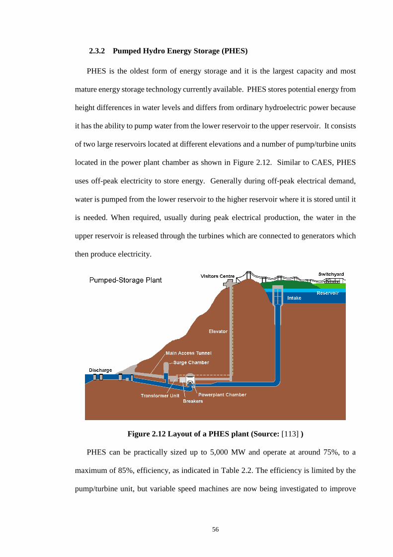
56

2.3.2 Pumped Hydro Energy Storage (PHES)

PHES is the oldest form of energy storage and it is the largest capacity and most

mature energy storage technology currently available. PHES stores potential energy from

height differences in water levels and differs from ordinary hydroelectric power because

it has the ability to pump water from the lower reservoir to the upper reservoir. It consists

of two large reservoirs located at different elevations and a number of pump/turbine units

located in the power plant chamber as shown in Figure 2.12. Similar to CAES, PHES

uses off-peak electricity to store energy. Generally during off‐peak electrical demand,

water is pumped from the lower reservoir to the higher reservoir where it is stored until it

is needed. When required, usually during peak electrical production, the water in the

upper reservoir is released through the turbines which are connected to generators which

then produce electricity.

Figure 2.12 Layout of a PHES plant (Source: [113] )

PHES can be practically sized up to 5,000 MW and operate at around 75%, to a

maximum of 85%, efficiency, as indicated in Table 2.2. The efficiency is limited by the

pump/turbine unit, but variable speed machines are now being investigated to improve

57

this [114]. The capital cost of PHES is in the region of €1200/kW but is very dependent

on a number of factors such as size, location and vicinity of the power grid. Currently,

approximately 140 GW of large scale energy storage is installed in electricity grids

worldwide [99]. PHES is currently the most widely implemented storage technology

worldwide, representing around 99% of the global grid scale energy storage capacity.

De-regulation and environmental concerns related to building large dams have influenced

the decline in the popularity of the PHES but in recent years increased demand for energy

storage installation rates are increasing interest in this technology again [100]. There are

several working examples of PHES plants exceeding 200 MW installed capacity

worldwide including Bath County, USA (2710 MW), Kannagawa, Japan (2700 MW),

Guangzhou, China (2400 MW), Lac des Dix, Switzerland (2009 MW) and Dinorwig, UK

(1800 MW) [100].

In the Republic of Ireland (ROI) there is currently only one large scale energy storage

plant, the Turlough Hill PHES plant. It was commissioned in 1974 and has an installed

capacity of 292 MW [115]. In 2011, Turlough Hill was unavailable due to maintenance

works and it was notable that during that time higher levels of wind curtailment were

reported than would otherwise have been expected [116]. In 2009, a new project was

launched entitled the Spirit of Ireland which promoted the large scale deployment of wind

farms and PHES in Ireland [117]. The PHES plants in the proposal would utilise U‐shaped

valleys along the Irish coastline as their upper reservoirs and the sea as their lower

reservoirs. However, no detailed analysis in terms of the size of the PHES plants and the

economic benefits of the proposal has been provided to date. Moreover, there is also a

proposal for a seawater PHES plant on the west coast of Ireland, which would store excess

wind energy from the surrounding wind farms and also have a direct transmission

58

connection from North Co.Mayo to the terminus of the East-West Interconnector in Co.

Dublin [118]. There is currently no large scale energy storage plant in Northern Ireland.

2.3.3 Energy storage in high renewable energy systems

Internationally, numerous studies have investigated the impact of different energy

storage technologies, in particular large scale energy storage in conjunction with high

renewable energy systems. Denholm et al. [119] investigated the role of energy storage

in the US electricity grid, focusing on the effects of large scale deployment of variable

RES, mainly wind and solar. Denholm et al. [119] state that ‘it is clear that high

penetration of variable generation increases the need for all flexibility options including

storage, and it also creates market opportunities for these technologies’. However, energy

storage has been difficult to sell into US markets, not only due to high costs, but because

of the array of services it provides and the difficulties in quantifying the value of these

services, particularly the operational benefits such as ancillary services. Therefore,

Denholm et al. [119] conclude that in order to examine the role of storage with variable

generation, continued analysis, improved data (i.e. representative techno-economic data

for energy storage technologies), and new techniques are required.

The stoRE study [96] as cited previously in Section 2.2.2 assessed the potential for

energy storage infrastructure, focusing on large scale energy storage technologies

including PHES and CAES plants at a European level for six target countries. The study

suggested the harmonisation of the European balancing energy markets in order to create

new trans-border means of income for energy storage plants. It also suggested the

development of an innovative support mechanism which could help them to contribute in

the high renewable power systems without distorting the energy market [96].

In Loisel et al. [21] the market value of PHES and CAES is examined in Germany

and France in 2030 in terms of wind generation confronted with a grid bottleneck. Loisel

59

et al. [21] indicate that PHES and CAES plants can be economically viable in the future

under favourable conditions. However, the extent to which the results indicated by Loisel

et al. [21] could be generalised to other countries depends on a number of factors such as

the flexibility of the generation mix, the strength of the transmission grid and

interconnection with other regions. Grunewald et al. [120] assessed, based on results

from an intermittency model, what issues policy makers may need to address for storage

(CAES, Hydrogen and Flow battery) to support future system balancing and energy

security in an economical way in GB. Grunewald et al. [120] indicated that under certain

assumptions large scale energy storage with long storage durations can become

commercially viable. In particular, for scenarios with high penetration of intermittent

generation, current storage technologies with low energy related capital costs can yield

positive returns but at the expense of efficiency. However, Grunewald et al. [120] cited

that the key areas of concern for energy storage developers and investors are the future

generation mix, technology development and market structures.

A number of Irish studies which have been undertaken examined the Irish energy

system with high renewable energy and large scale energy storage such as PHES and

CAES plants. For instance, Tuohy et al. [121] examined the Irish power system using

unit commitment model WILMAR for five different levels of installed wind capacity (6

GW, 7.5 GW, 9 GW, 10.5 GW and 12 GW) with and without PHES. The study indicated

that PHES reduced wind curtailment at high wind penetration levels and therefore,

captured more wind generation. However, even though it reduced curtailment and the

operating costs of the system, the high capital costs and inefficiencies of PHES were too

high to justify its development. Connolly et al. [122] also investigated how large scale

energy storage such as PHES can assist the integration of fluctuating RES by simulating

the Irish power system in the EnergyPLAN software tool. They determined that PHES

60

can feasibly increase the penetration of wind on the Irish power system and reduce its

operating costs [122]. However, Connolly et al. [122] state that the operational savings

are too small based on a conventional 6% interest rate and the predicted fuel prices for

2020 to warrant an investment in PHES. Their model was sensitive to changes in the

PHES capacities used, fuel prices, interest rates and the annual wind production [122]. In

Nyamdash et al. [123] the impact of combining wind generation and different types of

large scale energy storage (CAES, PHES, lead acid and vanadium redox batteries) on the

conventional thermal plant mix of the Irish power system is examined using 2006 SMP,

demand and wind generation data. Their main findings were that a merchant type storage

plant was unprofitable under an operational strategy of ‘buy-low and sell-high’ when

wind and load forecasts are assumed to be perfect and the network has no congestion

[123]. This is mainly due to the high capital costs and low round trip efficiencies of the

energy storage technologies, even though CAES was the most preferable technology

compared the other three in terms of capital costs [123]. Foley et al. [20] investigated

the techno-economic impact of a CAES plant in the SEM in 2020 using the PLEXOS

software tool. The key findings by Foley et al. [20] was that a CAES plant could

sufficiently optimise energy arbitrage opportunities, increase overall pool revenues for

most power producers and decrease CO2 emissions by 3% while sustaining a high

renewable energy system.

2.4 Modelling software tools

The key to performing reliable analyses of technologies such as energy storage in high

renewable energy systems is the use of modelling software tools which can produce

credible results when modelling a well-defined energy system. The main proprietary

modelling software tools used in different countries for power systems and market

modelling are PLEXOS, EMCAS, EnergyPLAN, WASP and WILMAR [124]. This

61

research is concerned with the Irish and British power systems, for which the most

common modelling software tools include: PLEXOS, BALMOREL, WILMAR and

EnergyPLAN [124], [125]. A brief outline of each software tool including their

commercial availability, applicability and input data availability based on a review of

literature and industry engagement is shown in Table 2.3. The following subsections

outline these tools in more detail.

Software

Tool

Software

Availability

Applicable

Energy

Sectors

Input Data

Availability

for Irish &

British

Systems

PLEXOS

Commercial/Free

for academic

institutions

Electricity &

Heat Good

BALMOREL Free to download

Electricity &

Heat (Partial) Limited

WILMAR Commercial

Electricity,

Heat (Partial)

& Transport

(Partial) Good

EnergyPLAN Free to download

Electricity,

Heat &

Transport Good

Table 2.3 Common electricity market modelling software tools

2.4.1 PLEXOS

PLEXOS was originally developed by Glenn Drayton of Drayton Analytics (now

called Energy Exemplar) in 1999 to model electricity markets. It is now an integrated

energy software tool supported by Energy Exemplar and is used for power and gas market

modelling worldwide [126]. PLEXOS is normally issued as a commercial modelling tool

but is free to academic institutions for non-commercial research. It can be used for power

and market analyses, market design and capacity expansion planning and portfolio

62

optimisation. As of January 2015, Energy Exemplar states PLEXOS installations (i.e.

licenced users) have exceeded 1025 at more than 165 sites in 36 countries [127].

PLEXOS is a proven power and natural gas market simulation tool which uses

mathematical programming, optimisation (Linear Relaxation, Rounded Relaxation and

Mixed Integer Programming) and stochastic techniques. Power and natural gas system

models developed in PLEXOS are scalable to thousands of generators (thermal, hydro

and renewable), transmission lines, well heads, pipelines, and storages in zonal or detailed

nodal network simulations. The main drawbacks of PLEXOS is the difficulty interacting

with third party software such as Matlab and R and compatibility issues in terms of

upgrading and downgrading of files for new releases of the software.

PLEXOS offers multiple horizon simulations, including 5 minute to hourly in order

to model and capture the effects of both the day-ahead and real time markets. It supports

multiple spatial analyses, from a full nodal network model to a zonal or regional model.

As such, it is capable of calculating the system electricity price, transmission congestion

costs and losses, and other market metrics. It also offers the same algorithms which TSOs

worldwide use to dispatch their markets and it is often used by the TSOs for internal and

external market analyses [128], [129].

PLEXOS has been widely used for the simulation of mixed integer unit commitment

and economic dispatch problems in the UK, Ireland, Poland, Turkey, Germany, as well

as projects outside of Europe, in particular in the USA, Africa and Australia [98], [130],

[131]. In particular, since 2007, PLEXOS has been used in Ireland by the TSOs Eirgrid

and SONI, Commission for Energy Regulation (CER) and SEM participants to validate

and forecast SEM outcomes [128], [132]. The CER [132] provides publically accessible

validated forecast PLEXOS models annually and documents the accuracy of these

models. Similarly, the UK’s TSO National Grid uses PLEXOS to calculate the efficiency

63

of the balancing mechanism in the BETTA market [129]. Moreover, it is considered by

academia as a well proven tool for policy analysis and development in several countries

[133]–[139].

2.4.2 BALMOREL

BALMOREL was originally developed as a collaboration project between research

and regulatory organisations in the Baltic Sea region financed by the Danish Energy

Agency [140]. The original purpose of this project was to develop a publically available

and flexible model for analysing the power and heat sectors in the Baltic Sea Region in

the face of increasing internationalisation of the electricity sector [141]. It was initially

used as a template for the development of Wind Power Integration in Liberalised

Electricity Markets (WILMAR) software tool and is today developed and distributed

under open source [124].

BALMOREL has been applied to projects in Ireland, Great Britain, Denmark,

Norway, Estonia, Latvia, Lithuania, Poland, Germany including projects outside of

Europe, in particular China, Eastern Africa and Canada [140]. Moreover, a comparative

validation analysis was conducted by Cleary et al. [142] between PLEXOS and

BALMOREL for the SEM and BETTA markets in 2012. It has been mainly used to

analyse security of electricity supply, wind power development, development of

international electricity markets, unit commitment, electric vehicle integration in the

power system, environmental policy evaluation and investigating the expansion of district

heating in Copenhagen.

BALMOREL has different versions used for various studies. Add-ons can be applied

for time aggregation, unit commitment, investments, policy requirements, etc. The model

has a number of different options for expanding the optimisation range. It can optimise a

64

year at a time, or it can optimise individual weeks. It also has an option for aggregating

time resolution to improve simulation time.

2.4.3 WILMAR

The WILMAR software tool was developed by Risoe National Laboratory as a

collaborative effort with industry and academic partners supported by the European

Commission under the fifth framework project [143]. The first version was issued in

2006 and was specifically created to analyse the integration of wind power for two power

pools; NordPool and the European Energy Exchange [124]. It was later modified to

analyse the Irish power system as part of the All-Island Grid Study in 2008 [94].

WILMAR is an advanced stochastic, mixed integer unit commitment and economic

dispatch model. The main functionality of the software tool is embedded in the scenario

tree tool and scheduling model [144]. The scenario tree tool is used to generate the

scenarios that are used as inputs in the scheduling model. The scenario tree tool can

produce forecasted time series for wind, demand and forced unit outages represented by

scenario trees. Each branch of the scenario tree represents a different forecast of wind and

demand including its probability of occurrence. The scheduling model minimises the

expected cost of the system over the optimisation horizon taking into account all the

scenarios generated by the scenario tree tool and subject to the generators operational

constraints.

WILMAR is primarily used to simulate global energy systems over a yearly time

horizon using an hourly or half hourly time step. Conventional and renewable generation

aswell as small and large scale energy storage can be incorporated in WILMAR with the

exception of solar thermal and geothermal [125]. WILMAR has been applied to projects

in Ireland, Great Britain and the Nordic countries. It has been mainly used to analyse

65

the integration of wind power, increased interconnection, generator cycling and energy

storage in electricity systems [121], [143], [145]–[147].

2.4.4 EnergyPLAN

EnergyPLAN was initially developed in 1999 by Aalborg University in Denmark

[125]. Since then it has been revised on a continuous basis with approximately ten

versions released to date. At present, it is developed and maintained by the Sustainable

Energy Planning Research Group at Aalborg University, Denmark. As of January 2015,

the EnergyPLAN website states downloads have exceeded 1200 [148]. EnergyPLAN

which is open source can be freely downloaded along with a range of training material.

The training period required can range from a few days up to a month, subject to the level

of complexity required [125].

EnergyPLAN simulates and optimises the operation of energy systems primarily on

an hourly basis. It is a user friendly tool designed in a series of tab sheets and programmed

in Delphi Pascal. It can incorporate complete national or regional energy systems

including heat and electricity aswell as the transport and industrial sectors. Conventional,

renewable, storage and transport technologies can be modelled by EnergyPLAN. It is a

deterministic input-output tool and general inputs are demand, renewable energy sources,

generator capacities and costs [125]. It optimises the operation of a given system as

opposed to tools which optimise investments in the system.

EnergyPLAN is used by academia, consultancies and policymakers for projects in

countries such as Ireland, Denmark, Italy, Greece, USA and China [148]. It has been

used to analyse the integration of wind power, 100% renewable energy penetration in

islanded systems, the effect energy storage in electricity systems, CHP and thermal

storage [149]–[153].

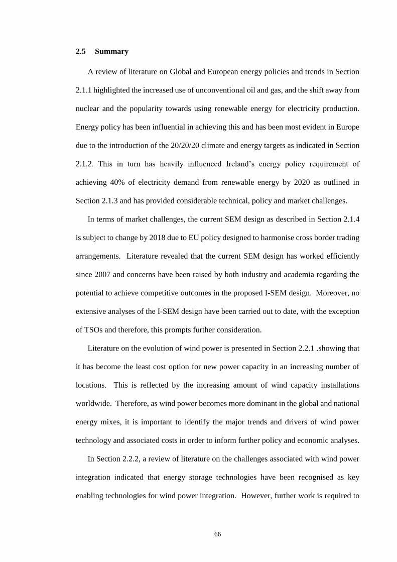
66

2.5 Summary

A review of literature on Global and European energy policies and trends in Section

2.1.1 highlighted the increased use of unconventional oil and gas, and the shift away from

nuclear and the popularity towards using renewable energy for electricity production.

Energy policy has been influential in achieving this and has been most evident in Europe

due to the introduction of the 20/20/20 climate and energy targets as indicated in Section

2.1.2. This in turn has heavily influenced Ireland’s energy policy requirement of

achieving 40% of electricity demand from renewable energy by 2020 as outlined in

Section 2.1.3 and has provided considerable technical, policy and market challenges.

In terms of market challenges, the current SEM design as described in Section 2.1.4

is subject to change by 2018 due to EU policy designed to harmonise cross border trading

arrangements. Literature revealed that the current SEM design has worked efficiently

since 2007 and concerns have been raised by both industry and academia regarding the

potential to achieve competitive outcomes in the proposed I-SEM design. Moreover, no

extensive analyses of the I-SEM design have been carried out to date, with the exception

of TSOs and therefore, this prompts further consideration.

Literature on the evolution of wind power is presented in Section 2.2.1 .showing that

it has become the least cost option for new power capacity in an increasing number of

locations. This is reflected by the increasing amount of wind capacity installations

worldwide. Therefore, as wind power becomes more dominant in the global and national

energy mixes, it is important to identify the major trends and drivers of wind power

technology and associated costs in order to inform further policy and economic analyses.

In Section 2.2.2, a review of literature on the challenges associated with wind power

integration indicated that energy storage technologies have been recognised as key

enabling technologies for wind power integration. However, further work is required to

67

understand how different market and policy frameworks may impact the deployment of

such technologies. A literature review of storage techno-economic parameters and their

impacts in conjunction with high renewable energy systems was conducted in Section

2.3. Literature revealed that high renewable energy systems, such as Irelands, increase

the need for flexibility options including large scale energy storage. In particular, a

number of Irish studies examined the Irish power system with high renewable energy

penetration and large scale energy storage such as PHES and CAES plants. However,

these studies focussed on simulating the current SEM design using various modelling

software tools. Currently, no simulation of the I-SEM design has been carried out by

academia, while the Irish TSOs have conducted some preliminary simulations.

A review of the main proprietary modelling software tools used in different countries

for power systems and market modelling were presented in Section 2.4. Existing

literature revealed that PLEXOS, BALMOREL, WILMAR and EnergyPLAN are the

most widely used software tools for modelling power systems and markets. In particular,

PLEXOS has been used by the TSOs, Regulators, SEM market participants and academia

for various Irish case studies given the availability of publically accessible PLEXOS

models of the SEM. However, a very limited number of these studies validated their

PLEXOS model outputs with actual SEM data, which is discussed further in Section 4.4.

68

3 THE COST OF WIND ENERGY

3.1 Introduction

As wind energy becomes a more important source of electricity generation in global

electricity markets, it is vital to identify the major trends and drivers of wind energy costs

(i.e. capital investment, operation and maintenance and financing costs). A better

understanding of the trends and cost drivers of the past, present and future cost of wind

energy both in Ireland and worldwide would help contribute to the national and global

policy debate in relation to the development and deployment of wind energy, respectively.

This chapter presents the technical and financial trends in the Irish wind industry since

2007 based on cost data and technical information collected from various sources, which

aligns with the first specific objective of this research as highlighted earlier in Section

1.3.The collected cost data can be used for the NPV analysis of wind generation as

indicated by step eight of the research methodology in Section 1.4. The following

subsections describe the cost of wind energy in Ireland and the associated methodology

and technology trends in more detail.

3.2 Methodology

The Sustainable Energy Authority of Ireland’s [154] wind farm database containing

installed capacity and year of connection for individual wind farms was used as a starting

point to create a detailed database of installed wind energy projects in Ireland between

2007 and 2012. Additional technical data were obtained from the Irish Wind Energy

Association (IWEA) including wind turbine make and model [155]. Performance data

such as full load hours and capacity factors were calculated based on aggregated county

wind energy production data provided by Eirgrid [156]. The wind production data at

quarter-hourly intervals from 143 wind farms operating during various time periods

69

2002–2013 was filtered and the yearly individual wind farm energy outputs were obtained

by using:

(3.1)

where:

Ei is the energy from wind farm i (MWh/annum)

Ec is the energy from county (MWh/annum)

Ci is the installed capacity of wind farm i

n is number of wind farms in county

The investment costs and operation and maintenance (O&M) costs were extracted

from financial reports filed by wind project owners with the Irish Companies Registration

Office [157], further details are provided in Sections 3.5 and 3.6. Financing costs were

obtained from literature and verified with major Irish lending institutions [158]. The

sample size for the technical and financial data for each year is contained in the appendix

in Duffy and Cleary [24].

After collection and verification of the data, the historical trends between 2007 and 2012

for wind projects in Ireland are presented in box and whiskers formats (with median

(horizontal line), average (diamond), 25th to 75th percentile (box), and minimum and

maximum (whiskers). The trend averages from the data represent the elements required

to calculate the Levelised Cost of Energy (LCOE) of a typical wind project in Ireland in

2008 and 2012. A detailed LCOE cash flow model developed by the Energy Research

Centre of the Netherlands (ECN) for use in the International Energy Agency (IEA) Wind

Task 26 [159] is used for the analysis presented in Section 3.9. It is acknowledged that

Irish wind projects can contribute to the costs associated with the DS3 and Grid 25

programmes for system services and grid development to integrate wind, respectively,

n

i

i

ici

C

CEE

1

70

however this is outside the scope of the analysis and is not included in the LCOE

calculation. The formulae used in the model’s calculation of LCOE are as follows:

(3.2)

(3.3)

where:

NPC is the life cycle net present cost

CC is the capital cost in year 0

MC is the maintenance cost in year i

OC is the operating cost in year i

DC is the decommissioning cost in year n

r is the discount rate (%)

Ei is the electricity produced in year i (kWh)

n is the lifespan (years)

3.3 Wind project features

Onshore wind energy projects in Ireland are generally in the form of clusters and

range from 2 to 19 wind turbines. Since 2007, the average wind project size in Ireland

has remained between 10 MW and 17 MW as shown in Figure 3.1. The largest wind

farms of between approximately 40 MW and 60 MW were installed between 2008 and

2011. The largest wind project size is 57 MW with 19 wind turbines. The average wind

project size was largest in 2008 and 2009 with 17 MW and 15 MW, respectively. In 2011,

average wind project size returned to 2007 levels.

n

i

i

i rE1

1 NPC = LCOE

nirDCr

11OC MC CC = NPC

n

1i

71

Figure 3.1 Wind project size trends from 2007 to 2012

The increasing trend of wind turbine capacity rating for each year since 2007 is

shown in Figure 3.2. The average wind turbine capacity rating increased almost two-fold

from 1.2 MW to 2.3 MW between 2007 and 2012. In 2010, the average wind turbine

capacity rating returned close to 2007 levels given that similar turbine sizes were installed

in these years compared to other years. However, there is no single apparent reason for

similar installed turbine sizes in 2007 and 2010. The maximum rated turbine capacity

was 3 MW, which occurred in 2009 and 2012. As the development of more advanced

wind turbine components has progressed and, in turn, larger turbines have evolved, wind

projects in Ireland have progressively used larger wind turbines. Moreover, empirical

evidence from the Irish wind energy industry suggests that larger wind turbines have been

used in recent years in order to ensure the available low wind resource locations were

financially viable.

72

Figure 3.2 Wind turbine capacity rating trends from 2007 to 2012

The trend since 2007 of increasing wind turbine rotor diameter (shown in Figure

3.3) coincided with the increase in wind turbine capacity referred to above. Generally, as

wind turbines became larger, so did their dimensions, such as the rotor diameter and hub

height. Between 2007 and 2012, the average wind turbine rotor diameter increased from

57 m to 78 m. In particular, between 2011 and 2012, the use of larger rotor diameters was

noticeable with a maximum of 100m in 2011. This increasing trend was reflective of the

emergence of larger wind turbines and wind projects in Ireland being sited in locations

with lower wind speeds as suggested by empirical evidence from the Irish wind energy

industry.

73

Figure 3.3 Wind turbine rotor diameter trends from 2007 to 2012

Average wind turbine hub height increased from 50 m in 2007 to 73 m in 2012 as

shown in Figure 3.4. Again, this trend can be attributed to wind projects being sited in

lower wind resource locations than previous years, thus requiring higher hub heights to

capture greater wind speeds.

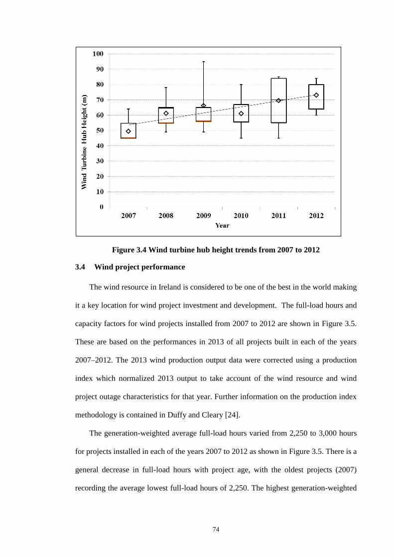
74

Figure 3.4 Wind turbine hub height trends from 2007 to 2012

3.4 Wind project performance

The wind resource in Ireland is considered to be one of the best in the world making

it a key location for wind project investment and development. The full-load hours and

capacity factors for wind projects installed from 2007 to 2012 are shown in Figure 3.5.

These are based on the performances in 2013 of all projects built in each of the years

2007–2012. The 2013 wind production output data were corrected using a production

index which normalized 2013 output to take account of the wind resource and wind

project outage characteristics for that year. Further information on the production index

methodology is contained in Duffy and Cleary [24].

The generation-weighted average full-load hours varied from 2,250 to 3,000 hours

for projects installed in each of the years 2007 to 2012 as shown in Figure 3.5. There is a

general decrease in full-load hours with project age, with the oldest projects (2007)

recording the average lowest full-load hours of 2,250. The highest generation-weighted

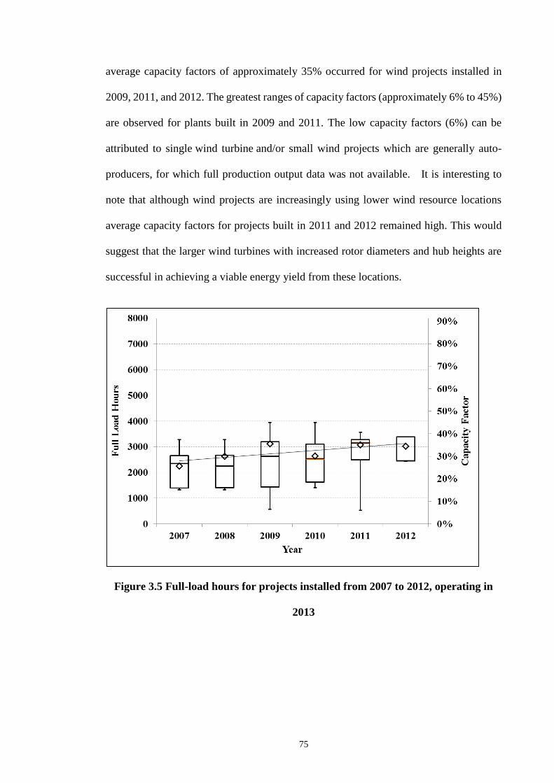
75

average capacity factors of approximately 35% occurred for wind projects installed in

2009, 2011, and 2012. The greatest ranges of capacity factors (approximately 6% to 45%)

are observed for plants built in 2009 and 2011. The low capacity factors (6%) can be

attributed to single wind turbine and/or small wind projects which are generally auto-

producers, for which full production output data was not available. It is interesting to

note that although wind projects are increasingly using lower wind resource locations

average capacity factors for projects built in 2011 and 2012 remained high. This would

suggest that the larger wind turbines with increased rotor diameters and hub heights are

successful in achieving a viable energy yield from these locations.

Figure 3.5 Full-load hours for projects installed from 2007 to 2012, operating in

2013

76

3.5 Investment costs

The capacity-weighted average investments costs of Irish wind projects ranged from

€990/kW to €1,658/kW (2012 prices) between 2007 and 2012 as shown in Figure 3.6.

Overall the cost trend was upwards over the period, although in 2011 average costs fell.

It did not prove possible to obtain a breakdown of the individual cost components of wind

projects investment costs. However, empirical evidence from the Irish wind energy

industry suggests that wind turbine and civil works costs (i.e. due to reduced demand in

Irish construction market) may be declining, resulting in an overall decrease in investment

costs. However, this is not clearly reflected in the data obtained in this study, which is

now a few years out of date. There is no single obvious explanation for the observed

upward cost trend. This may be due to a variety of factors such as: tight construction

market conditions (particularly 2007/8 feeding into 2009); high international demand for

wind turbines; increased rotor diameters and associated increased turbine costs; and other

cost components such as higher grid connection costs.

In terms of projections beyond 2012 and 2013, several projects in 2014 will be located

in the midlands of Ireland where suitable land for wind project development is available.

These areas of land tend to have lower wind speeds and may require low specific power

turbines in order to ensure financial viability. It was suggested by industry sources that

investment costs may vary between €1,400/kW and €1,600/kW for large-scale (>5MW)

wind projects in 2014, which was based on market conditions at the time.

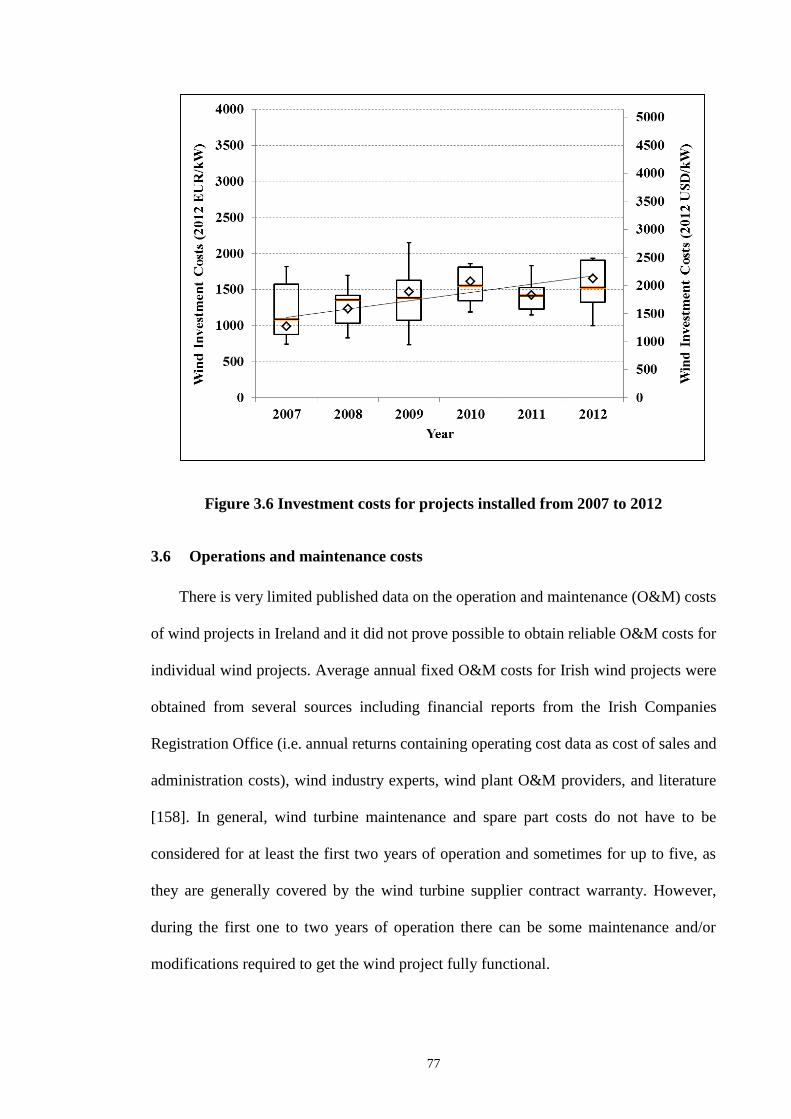
77

Figure 3.6 Investment costs for projects installed from 2007 to 2012

3.6 Operations and maintenance costs

There is very limited published data on the operation and maintenance (O&M) costs

of wind projects in Ireland and it did not prove possible to obtain reliable O&M costs for

individual wind projects. Average annual fixed O&M costs for Irish wind projects were

obtained from several sources including financial reports from the Irish Companies

Registration Office (i.e. annual returns containing operating cost data as cost of sales and

administration costs), wind industry experts, wind plant O&M providers, and literature

[158]. In general, wind turbine maintenance and spare part costs do not have to be

considered for at least the first two years of operation and sometimes for up to five, as

they are generally covered by the wind turbine supplier contract warranty. However,

during the first one to two years of operation there can be some maintenance and/or

modifications required to get the wind project fully functional.

78

For this analysis, an average fixed O&M cost of €55/kW/yr (expressed as capacity-

based with performance guaranteed in terms of time) was estimated between 2007 and

2012 over the 20-year wind projects lifetime based primarily on industry sources. This

includes land rent, maintenance by the turbine manufacturer, insurance, county council

rates and transmission use of system (TUOS) charges. TUOS charges are charges

imposed by the Irish TSO on generators for their use of the national grid. Empirical

evidence from the Irish wind energy industry suggests that since 2007, O&M costs have

increased mainly due to land rent, county council rates, and TUOS charges.

3.7 Financing costs

During the period 2007–2012, there were a limited number of active lenders for wind

projects in Ireland as a result of the great recession and a national financial crisis. Due to

the financial crisis, lenders have been very selective in the project types and project

developers they have financed. There is limited published data on financing costs for Irish

wind projects and it did not prove possible to obtain these costs for individual projects.

Based on interviews (consisting of discussions on the main financing parameters between

2007 and 2012) with two of the major Irish lending institutions and a literature review,

representative financing costs were compiled as shown in Table 3.1.

2008 2012

Return on equity (%) 14 14

Return on debt (%) 6 6

Equity share (%) 20 20

Debt share (%) 80 80

Loan duration (years) 15 15

Corporate tax rate (%) 12.5 12.5

WACC (after-tax,

nominal) 7 7

Table 3.1 Wind project financing parameters in 2008 and 2012

79

All values are presented in after-tax nominal terms, but subsequent LCOE

calculations are formulated in after-tax real terms. The Irish Corporate Tax Rate (CTR)

of 12.5% is one of the lowest in Europe applicable on trading income of Irish resident

companies and Irish branches of foreign companies. The Return on Equity (RoE) was

estimated to be 14% while 6% was taken as the interest Return on Debt. Equity (E) and

Debt (D) shares of 20% and 80% are thought to have remained stable between 2007 and

2012 This produces an after-tax, nominal Weighted Average Cost of Capital (WACC) of

7% using Equation (3.4) for both 2008 and 2012 wind projects.

(3.4)

3.8 Policy incentives

A variety of incentives have been used in the wind industry over the last 25 years.

However, the current Renewable Energy Feed in Tariff (REFIT) has been in place for

eight years and has thus provided a relatively stable investment environment. The REFIT

scheme was delivered in two phases [160]. REFIT 1 contracts were awarded between

2006 and 2010, and qualifying projects can be executed up to the end of 2015. The

replacement REFIT 2 scheme was opened for applications in March 2012 and has a

deadline of the end of 2017 for the energizing of qualifying projects. The payments

defined under REFIT 1 and REFIT 2 are identical, but the arrangements for market

compensation accruing to Power Purchase Agreements (PPA) counterparties are

modified under REFIT 2. The REFIT scheme for wind is funded through a European

Commission (EC) state-aid sanctioned, Public Service Obligation (PSO) levy on all

electricity consumers. The total PSO amount levied in 2012/2013 was €131 million; peat

generation, provision for security of supply generation, and renewable electricity

generation accounted for 39%, 19%, and 42% of the PSO, respectively [161].

CTR) -(1*RoD* D +RoE*D)-(1 = WACCnominal tax,-After

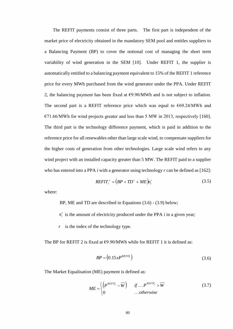
80

The REFIT payments consist of three parts. The first part is independent of the

market price of electricity obtained in the mandatory SEM pool and entitles suppliers to

a Balancing Payment (BP) to cover the notional cost of managing the short term

variability of wind generation in the SEM [10]. Under REFIT 1, the supplier is

automatically entitled to a balancing payment equivalent to 15% of the REFIT 1 reference

price for every MWh purchased from the wind generator under the PPA. Under REFIT

2, the balancing payment has been fixed at €9.90/MWh and is not subject to inflation.

The second part is a REFIT reference price which was equal to €69.24/MWh and

€71.66/MWh for wind projects greater and less than 5 MW in 2013, respectively [160].

The third part is the technology difference payment, which is paid in addition to the

reference price for all renewables other than large scale wind, to compensate suppliers for

the higher costs of generation from other technologies. Large scale wind refers to any

wind project with an installed capacity greater than 5 MW. The REFIT paid to a supplier

who has entered into a PPA i with a generator using technology r can be defined as [162]:

(3.5)

where:

BP, ME and TD are described in Equations (3.6) - (3.9) below;

r

in is the amount of electricity produced under the PPA i in a given year;

r is the index of the technology type.

The BP for REFIT 2 is fixed at €9.90/MWh while for REFIT 1 it is defined as:

(3.6)

The Market Equalisation (ME) payment is defined as:

(3.7)

0

WPME

jREFIT

otherwise

WPif jREFIT

115.0REFIT

xPBP

r

i

rr

i nMETDBPREFIT

81

If the average wholesale SEM price W is less than the REFIT reference price

jREFITP (where j indexes either REFIT 1 or 2), the supplier receives the difference between

the two prices [162]. Wind projects enter into a 15-year PPA with electricity suppliers at

a negotiated price per unit of electricity. The supplier then sells the electricity into the

SEM pool. If the SEM price a supplier receives for each half-hourly trading period during

the year is less than the jREFITP , then the difference is paid through the PSO mechanism.

When the SEM price a supplier receives for each trading period during the year is higher

than the jREFITP , those generators in the AER scheme pay back the additional market

revenue to the PSO fund, while generators in the REFIT scheme retain the market revenue

[163].

The technology difference payment TDr depends on the REFIT phase. Under

REFIT 1, Equation (3.8 indicates that the technologies depend on PPPA, the price per

MWh specified in the PPA between the generator and supplier; Gr the relevant technology

reference price for each generation type r; and the appropriate REFIT reference price

jREFITP [162].

(3.8)

For technologies that fall under REFIT 2, the technology payment depends on the

average wholesale SEM priceW , PPPA and Gr as shown in Equation (3.9). In practice it

is unlikely that PPPA would be lower than Gr [162].

(3.9)

0

WP

WG

TD PPA

r

r

1

1

REFITPPA

rPPAREFIT

rPPA

PPif

GPPif

GPif

0

1

1

REFITPPA

REFITr

r PP

PG

TD

WPif

GPWif

WGPif

PPA

rPPA

rPPA

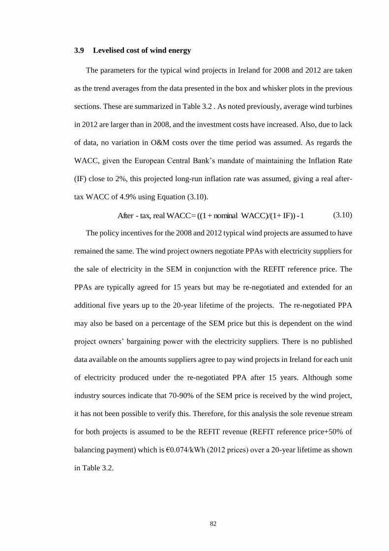
82

3.9 Levelised cost of wind energy

The parameters for the typical wind projects in Ireland for 2008 and 2012 are taken

as the trend averages from the data presented in the box and whisker plots in the previous

sections. These are summarized in Table 3.2 . As noted previously, average wind turbines

in 2012 are larger than in 2008, and the investment costs have increased. Also, due to lack

of data, no variation in O&M costs over the time period was assumed. As regards the

WACC, given the European Central Bank’s mandate of maintaining the Inflation Rate

(IF) close to 2%, this projected long-run inflation rate was assumed, giving a real after-

tax WACC of 4.9% using Equation (3.10).

(3.10)

The policy incentives for the 2008 and 2012 typical wind projects are assumed to have

remained the same. The wind project owners negotiate PPAs with electricity suppliers for

the sale of electricity in the SEM in conjunction with the REFIT reference price. The

PPAs are typically agreed for 15 years but may be re-negotiated and extended for an

additional five years up to the 20-year lifetime of the projects. The re-negotiated PPA

may also be based on a percentage of the SEM price but this is dependent on the wind

project owners’ bargaining power with the electricity suppliers. There is no published

data available on the amounts suppliers agree to pay wind projects in Ireland for each unit

of electricity produced under the re-negotiated PPA after 15 years. Although some

industry sources indicate that 70-90% of the SEM price is received by the wind project,

it has not been possible to verify this. Therefore, for this analysis the sole revenue stream

for both projects is assumed to be the REFIT revenue (REFIT reference price+50% of

balancing payment) which is €0.074/kWh (2012 prices) over a 20-year lifetime as shown

in Table 3.2.

1-IF))+ WACC)/(1nominal+((1 = WACCreal tax,-After

83

2008 2012

Unit size (MW) 1.5 2.1

Number of turbines (no.) 9 6

Rotor Diameter / Hub height

(m/m) 64/58 76/73

Production (full-load hours) 2,653 3,194

Investment costs (€2012/kW) 1,226 1,689

O&M costs fixed (€2012/kW/yr) 55 55

WACC (after-tax, real) (%) 4.9 4.9

Corporate Tax Rate (%) 12.5 12.5

REFIT revenue (€2012/kWh) 0.074 0.074

REFIT policy period (years) 20 20

Depreciation period (years) 20 20

Economic life (years) 20 20

Table 3.2 Wind project technical and financial features in 2008 and 2012

The LCOE (defined by Equation (3.2) is calculated for each project in 2008 and 2012

using the ECN LCOE cash flow model developed for use in the IEA Wind Task 26 [159].

A common assumption across all countries participating in the IEA Task 26 is that the

LCOE estimates include a 20-year straight-line depreciation of 100% of the investment

costs; this is assumed to be representative of generic tax treatment across all countries for

any asset and is also assumed for this research. Furthermore, tax treatment such as

accelerated depreciation specific to wind energy is considered a policy incentive and for

the purposes of this research, the REFIT is considered the only policy incentive for Irish

wind projects.

The LCOE for each typical project in 2008 and 2012 is shown in Table 3.3. The

difference between the estimated LCOE and the REFIT revenue is the required revenue

which represents the impact of the Irish REFIT support scheme. A positive revenue

required value indicates insufficient revenues to cover all wind project costs whereas a

negative value implies all costs are covered. For the 2008 project, the LCOE of

€59.45/MWh is covered by €74.43/MWh in the form of the REFIT revenue over the

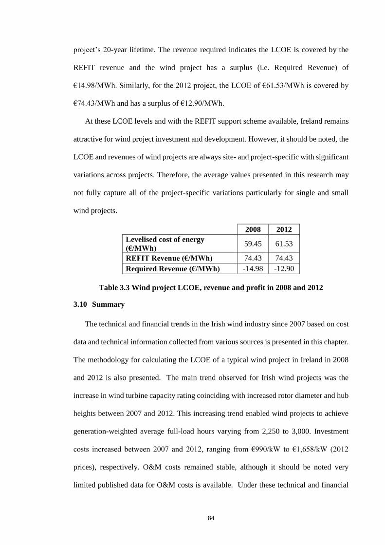
84

project’s 20-year lifetime. The revenue required indicates the LCOE is covered by the

REFIT revenue and the wind project has a surplus (i.e. Required Revenue) of

€14.98/MWh. Similarly, for the 2012 project, the LCOE of €61.53/MWh is covered by

€74.43/MWh and has a surplus of €12.90/MWh.

At these LCOE levels and with the REFIT support scheme available, Ireland remains

attractive for wind project investment and development. However, it should be noted, the

LCOE and revenues of wind projects are always site- and project-specific with significant

variations across projects. Therefore, the average values presented in this research may

not fully capture all of the project-specific variations particularly for single and small

wind projects.

2008 2012

Levelised cost of energy

(€/MWh) 59.45 61.53

REFIT Revenue (€/MWh) 74.43 74.43

Required Revenue (€/MWh) -14.98 -12.90

Table 3.3 Wind project LCOE, revenue and profit in 2008 and 2012

3.10 Summary

The technical and financial trends in the Irish wind industry since 2007 based on cost

data and technical information collected from various sources is presented in this chapter.

The methodology for calculating the LCOE of a typical wind project in Ireland in 2008

and 2012 is also presented. The main trend observed for Irish wind projects was the

increase in wind turbine capacity rating coinciding with increased rotor diameter and hub

heights between 2007 and 2012. This increasing trend enabled wind projects to achieve

generation-weighted average full-load hours varying from 2,250 to 3,000. Investment

costs increased between 2007 and 2012, ranging from €990/kW to €1,658/kW (2012

prices), respectively. O&M costs remained stable, although it should be noted very

limited published data for O&M costs is available. Under these technical and financial

85

features, typical Irish wind projects in 2008 and 2012 achieved LCOEs of €59.45/MWh

and €61.53/MWh, respectively. At these LCOE levels and with the REFIT support

scheme available, Ireland remains attractive for wind project investment and

development. However, the LCOE of wind projects are always site- and project-specific

with significant variations across projects. Therefore, the average values presented in this

chapter may not capture all of the project specific variations. In the next chapter, the

methodology implemented for the 2012 unit commitment and economic dispatch

PLEXOS base case model including the main model input assumptions is presented.

86

4 BASE MODEL

4.1 Introduction

In this chapter, the methodology implemented for the 2012 PLEXOS base case model

is presented, which aligns with steps three and four of the research methodology in

Section 1.4. Initially a representation of the SEM and BETTA market in 2012 was created

in PLEXOS as the base year model given that detailed data were available for that year.

PLEXOS as outlined in Section 2.4.1 is an integrated energy software tool used for power

and gas market modelling worldwide. PLEXOS has been used extensively by industry

and academia for policy analysis and development in both Ireland and the UK [133]–

[139]. Therefore, PLEXOS versions 6.4 R02 was used to build and run the models for

this analysis. The 2012 base model was populated with the individual generator technical

and commercial characteristics and used to simulate the markets under normal conditions

for that year. The 2012 base model was then validated using market data in that year.

The analysis employed a deterministic model using the assumptions as described in

Section 4.3. It assumed perfect foresight (i.e. fixed time series profiles are used) for all

variable renewable generation and system demand with no design or rules changes to the

SEM and BETTA markets. The analysis therefore applied the current SEM rules and

assumed the current bidding principles and methodology for calculating the various cost

and revenue streams remained unchanged. The BETTA market was treated as a

centralised pool market with the assumption it produces similar outcomes to the bilateral

trading arrangements which exist in the current market. The following subsections

describe the modelling software, base model description and assumptions, and base

model validation in more detail.

87

4.2 Base model description

A number of publicly available sources were used for the creation of the 2012

PLEXOS base model. The CER validated forecast model of 2011-2012 was used as a

starting point from which the 2012 PLEXOS model for this analysis was developed [132].

The 2012 model was populated with the individual generator technical and commercial

characteristics which have signed agreements and confirmed dates to connect to the SEM

[164]. The demand and wind capacity for 2012 were obtained from the CER [132] and

cross-checked with Eirgrid and SONI [164]. A detailed model of the BETTA market was

created using the Deane et al. [165] model as a starting point. The model was populated

with the individual generator technical characteristics based on the reported installed

capacities from DECC [166]. The model also includes interconnector flows between

SEM and BETTA as well as flows from the simplified French and Dutch markets in the

form of flows produced by a BALMOREL model from Cleary et al. [142].

The model treats the SEM and BETTA markets as centralised pool markets. The

BETTA market is particularly difficult to model given the bilateral contracts which exist

between generators and suppliers and the strategic bidding practices by vertically

integrated utilities. Moreover, it is acknowledged there will be discrepancies between the

PLEXOS model outputs and the actual market outputs; this is discussed further in Section

4.4. However, it is assumed that the centralised pool approach will yield similar outcomes

to the bilateral trading arrangements in the BETTA market. This approach has also been

adopted by Curtis et al. [167] and Deane et al. [168].

The PLEXOS base model simulation engine reads the input data such as system

demand and wind data as shown in Figure 4.1 [133]. The graphical user interface of

PLEXOS consists of a modern ribbon style of menus. The menu icons are organised in

88

main tabs “File”, “Home” and “Window”. The ribbon consolidates all functionality to

create and edit databases, run models and review simulation results.

Figure 4.1 PLEXOS system modelling structure (Source: [133])

PLEXOS simulates 365 individual daily optimisations at 48 half-hourly intervals

while ensuring the generation portfolio meets demand at least cost while taking into

account the individual generator’s techno-economic parameters as in shown in Equation

(4.1) [139]:

(4.1)

subject to the constraints:

(4.2)

(4.3)

where:

di is the binary number indicating whether a generator has been scheduled (1) or

not (0)

Ci is the generation cost of generator i (€)

Pi is the power output of generator i (MW)

Pd is the system demand (MW)

1,0,min48

1 1

i

t

uplift

N

i

iii dCPCd

N

i

di PP1

maxmin

iii PPP

89

Pimin and Pi

max are the power output limits of generator i (MW)

Cuplift is the uplift cost which is determined from start-up and no-load costs

N is the number of dispatchable generators

i is the index of generators

Prior to dispatch, the model calculates the availability of each generator for the year

taking into account their planned and unplanned maintenance, which is described further

in subsection 4.3.1. Similar to the SEM and BETTA markets, the model calculates the

electricity prices and generator output schedules for each half hour trading period,

therefore providing an accurate representation of the dispatch of generators in both

markets. Further details of the base model equations are shown in Appendix A and the

typical equations for modelling the SEM are also outlined in Deane et al. [135]. The

following subsections describe the model assumptions in more detail.

4.3 Base model assumptions

4.3.1 Generation portfolio

The base model incorporates detailed characteristics for individual generator types

for both the SEM and BETTA markets. Table 4.1 shows the aggregated conventional

generation portfolio for the SEM and BETTA markets in 2012. The gas- and coal-fired

generators provide the largest contribution to the generation portfolio in both markets.

Subsequently, gas has been the predominant marginal generator type in both markets and

a high correlation exists between the price of gas and the electricity prices in the markets

[132]. A restriction on the number of operating hours of the BETTA coal generators was

enforced to reflect the Large Combustion Plant Directive (LCPD, 2001/80/EC) [169],

therefore a maximum annual load factor of 38% was set in both models. Nuclear

generation in the UK also experienced reduced operating hours due to technical problems

and annual load factors of 80% for 2012 were set in both models.

90

Generator type SEM BETTA

Coal 1,331 25,774

Gas 5,478 36,070

Oil 804 4,032

Nuclear 0 9,231

Distillate Oil 640 0

Peat 346 0

Total (MW) 8,598 75,107

Table 4.1 2012 aggregated conventional generation portfolio capacity (MW)

The renewable generation portfolio for the 2012 SEM and BETTA markets is shown

in Table 4.2. Onshore and offshore wind provides the predominant share of the renewable

generation portfolio in both markets. There is only 25 MW of installed offshore wind

capacity from a single wind project in the SEM compared to 2,995 MW in the BETTA

market. The modelling approach for wind generation is described further in Section 4.3.2.

Generator type SEM BETTA

Hydropower 216 1,680

Pumped hydro storage 292 2,828

Onshore wind 2,224 5,438

Offshore wind 25 2,995

Solar PV 0 1,700

Solid Biomass 0 1,014

Biogas 0 1,223

Waste 17 0

Total (MW) 2,774 16,878

Table 4.2 2012 aggregated renewable generation portfolio capacity (MW)

Hourly profiles for solar PV were obtained from Deane et al. [165] and implemented

in the model. Although, the solar profiles are in hourly intervals, the PLEXOS simulator

interpolates between each hourly data point to reflect each market’s half hourly trading

period, this simplification could lead to an under and/or over estimation of solar

generation. The pumped hydro storage generators are optimised and dispatched based

on the pumping and generation cycles which are subject to the head and tail reservoir

capacities. The hydro generators in the SEM are optimised based on fixed daily hydro

91

resource limits for each month in 2012. In the BETTA market, the hydro generators are

assigned a 36% annual capacity factor as detailed hydro resource limits were not

publically available. The biogas and biomass generators are assigned 56% and 75%

annual capacity factors set within the model based on historic market data, respectively

[166].

Embedded generation in the SEM, which is classified as small scale generation such

as Combined Heat and Power (CHP) and small scale renewables connected to commercial

properties is implemented in the base model. The embedded generation with an installed

capacity ranging from 112 to 211 MW follows an hourly profile which is different for

weekdays and weekends. The complete transmission network is not included in the

model and localised network constraints are not modelled. Instead, the model consists of

two separate nodes representing the SEM and BETTA markets, with all the generator

types assigned to the respective node. The model applies on average 2% transmission

losses (as per the TSOs recommendations) to all generator types to account for the

possible losses within the SEM and BETTA markets [170].

4.3.2 Wind generation

Wind generation in the SEM is modelled in the base model under the assumption of

perfect foresight in aggregated form, split into 13 regions as shown in Figure 4.2. Each

region has an associated hourly capacity factor profile which represents the wind

availability in that region for a typical meteorological year obtained from CER [132].

92

Figure 4.2 Base model wind regions (Source: [132])

The onshore and offshore wind for the BETTA market is represented by hourly

profiles for the GB region for the year taken from Deane et al. [165]. Moreover, British

wind power output is assumed to lag Irish wind power output by 3 hours, meaning that

the wind appears in GB later than it has appeared in Ireland. Similar studies have used a

time lag ranging from 2-4 hours [18], [139]. Although, the wind profiles are in hourly

intervals, the PLEXOS simulator interpolates between each hourly data point to reflect

each market’s half hourly trading period, this simplification could lead to an under and/or

over estimation of wind generation.

4.3.1 Maintenance schedules

The planned and unplanned maintenance outage schedules for each generator during

the year are taken into account. The former is assigned manually based on the 2012

schedule and the latter is modelled as a random event using forced outage rates and mean

time to repair from CER [132] for the SEM in the model. For the BETTA market, planned

maintenance outage schedules were not publically available; therefore maintenance

outage schedules for each generator are modelled as a random event based on the forced

93

outage rates and mean time to repair from Deane et al. [165]. The frequency and duration

of the outages are determined randomly by the base model using a method known as

Convergent Monte Carlo. The Convergent Monte Carlo method works by pre-filtering

patterns of outages to eliminate statistically unlikely outcomes while ensuring generators

are being scheduled according to the status of the SEM and BETTA markets capacity

margins (i.e. available capacity over and above the capacity needed to meet demand).

The use of pre-filtering involves selecting a number of generator outage patterns by

computing a chi-square statistic which chooses the pattern closest to the expected

outcome for each final pattern used in the simulation.

4.3.2 System demand

The system demand for each half hourly period in 2012 is included in the base model

based on the 2012 system demand profile from CER [132]. The annual demand is

estimated to be 36.5 TWh with a peak demand of 6.5 GW and 308.6 TWh with a peak

demand of 55.8 GW for SEM and BETTA markets, respectively. Therefore, the demand

in the BETTA market is approximately nine times greater than the SEM and this is

reflected by the total generation portfolio capacity in each market.

4.3.3 Interconnectors

The Moyle Interconnector (MI) links the SEM to BETTA market and flows on the

interconnector are largely driven by arbitrage of the relative prices in the two markets.

There is uncertainty in relation to the actual maximum import and export capacity of the

MI for the foreseeable future due to an undersea cable fault [109]. Therefore, in the base

model, the MI is assumed to be limited to exporting 250 MW and importing 450 MW

November-March and 410 MW April-October all year. The BritNed interconnector and

England-France interconnector (IFA) links the BETTA market to the Dutch and French

94

markets, respectively. The import and export flows for the BritNed and IFA

interconnectors are fixed within the base model based on historic 2012 data [171]. This

simplified approach was adopted as it reduces the need to create a detailed representation

of the Dutch and French markets and significantly reduces computational time.

4.3.4 Cost input data

Fuel prices for the ROI, NI and GB are based on quarterly predictions for 2012 as

shown in Table 4.3 from two main sources [163], [172]. The fuel prices are based on the

quarterly spot market prices in 2012 and include transportation costs to the generator. The

transportation costs are calculated using a fuel delivery calculator developed by the CER

[132].

Fuel price (€/GJ)

Fuel type Q1

2012

Q2

2012

Q3

2012

Q4

2012

NI Gas 8.01 7.73 7.74 8.60

RoI Gas 7.98 7.69 7.70 8.57

NI Oil 17.20 16.10 16.72 15.41

RoI Oil 17.55 16.45 17.07 15.75

NI Coal 3.51 3.11 3.17 3.06

RoI Coal 3.10 2.70 2.76 2.65

NI Distillate 21.63 21.26 21.90 20.50

RoI

Distillate 21.99 21.62 22.25 20.86

GB Coal 3.37 3.33 3.05 2.93

GB Oil 16.11 15.63 16.56 15.24

GB Gas 7.83 7.28 7.21 7.93

GB Diesel 16.11 15.63 16.56 15.24

GB Nuclear 0.71 0.71 0.71 0.71

GB Biomass 1.53 1.53 1.53 1.53

GB

Bioenergy 1.53 1.53 1.53 1.53

Table 4.3 Quarterly fuel prices for 2012 (Source: [163], [172])

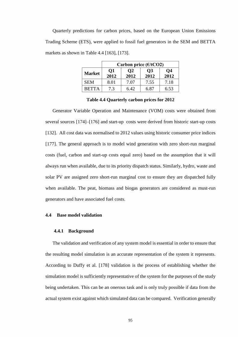
95

Quarterly predictions for carbon prices, based on the European Union Emissions

Trading Scheme (ETS), were applied to fossil fuel generators in the SEM and BETTA

markets as shown in Table 4.4 [163], [173].

Carbon price (€/tCO2)

Market Q1

2012

Q2

2012

Q3

2012

Q4

2012

SEM 8.01 7.07 7.55 7.18

BETTA 7.3 6.42 6.87 6.53

Table 4.4 Quarterly carbon prices for 2012

Generator Variable Operation and Maintenance (VOM) costs were obtained from

several sources [174]–[176] and start-up costs were derived from historic start-up costs

[132]. All cost data was normalised to 2012 values using historic consumer price indices

[177]. The general approach is to model wind generation with zero short-run marginal

costs (fuel, carbon and start-up costs equal zero) based on the assumption that it will

always run when available, due to its priority dispatch status. Similarly, hydro, waste and

solar PV are assigned zero short-run marginal cost to ensure they are dispatched fully

when available. The peat, biomass and biogas generators are considered as must-run

generators and have associated fuel costs.

4.4 Base model validation

4.4.1 Background

The validation and verification of any system model is essential in order to ensure that

the resulting model simulation is an accurate representation of the system it represents.

According to Duffy et al. [178] validation is the process of establishing whether the

simulation model is sufficiently representative of the system for the purposes of the study

being undertaken. This can be an onerous task and is only truly possible if data from the

actual system exist against which simulated data can be compared. Verification generally

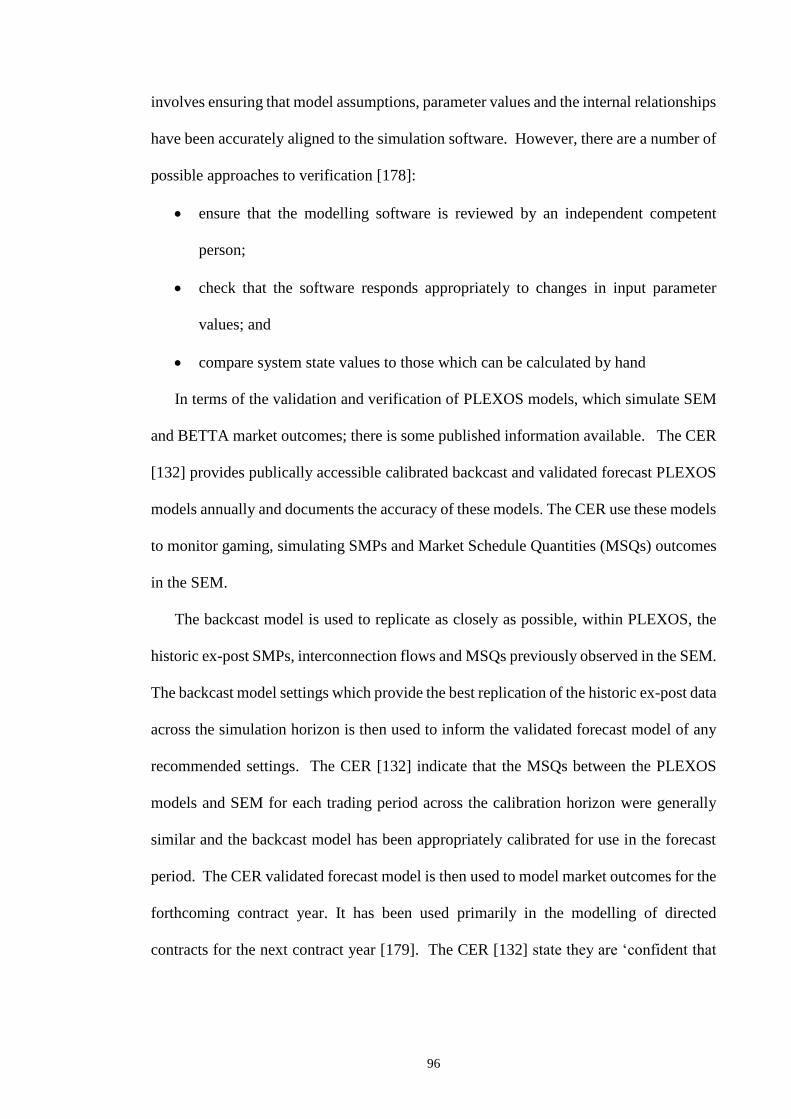
96

involves ensuring that model assumptions, parameter values and the internal relationships

have been accurately aligned to the simulation software. However, there are a number of

possible approaches to verification [178]:

ensure that the modelling software is reviewed by an independent competent

person;

check that the software responds appropriately to changes in input parameter

values; and

compare system state values to those which can be calculated by hand

In terms of the validation and verification of PLEXOS models, which simulate SEM

and BETTA market outcomes; there is some published information available. The CER

[132] provides publically accessible calibrated backcast and validated forecast PLEXOS

models annually and documents the accuracy of these models. The CER use these models

to monitor gaming, simulating SMPs and Market Schedule Quantities (MSQs) outcomes

in the SEM.

The backcast model is used to replicate as closely as possible, within PLEXOS, the

historic ex-post SMPs, interconnection flows and MSQs previously observed in the SEM.

The backcast model settings which provide the best replication of the historic ex-post data

across the simulation horizon is then used to inform the validated forecast model of any

recommended settings. The CER [132] indicate that the MSQs between the PLEXOS

models and SEM for each trading period across the calibration horizon were generally

similar and the backcast model has been appropriately calibrated for use in the forecast

period. The CER validated forecast model is then used to model market outcomes for the

forthcoming contract year. It has been used primarily in the modelling of directed

contracts for the next contract year [179]. The CER [132] state they are ‘confident that

97

the dataset used in building the forecast model provides a reasonable and consistent

representation of the market’.

A recent study by Clancy et al. [180] validated a PLEXOS model with actual 2012

SEM data. The predicted share of each generation type from the PLEXOS model

simulations is compared to the actual 2012 SEM data including the accuracy of generator

dispatch predicted from the model relative to the actual recorded SEM data at a daily

resolution. Clancy et al. [180] observed that the simulated MSQs of Combined Cycle

Gas Turbines (CCGTs), coal, peat and peaking generators were 61%, 29%, 9% and 0.6%,

respectively, compared to the actual shares of 62%, 27%, 9% and 1% in 2012. However,

Clancy et al. [180] did not conduct a comparative validation analysis between the

PLEXOS model and actual SEM SMPs in 2012.

Denny [134] considered validation of the SMPs between a PLEXOS model and actual

SEM in 2008 but not the MSQs. Denny [134] indicates the accuracy of the PLEXOS

model by comparing the predicted average SMPs in the first four months of the SEM to

the actual average SMPs. Deane [181] only examined the 2008 SEM dispatch profile of

the PHES plant Turlough Hill and compared it to the modelled dispatch profile from a

PLEXOS model. It was determined that the simulated profile of Turlough Hill followed

quite closely the actual SEM profile with annual generation of 255 GWh and 265 GWh,

respectively [181]. Edmunds et al. [182] developed a 2012 PLEXOS model of the

BETTA market and verified the main model input parameters such as generator installed

capacities against a number of data sources to ensure its accuracy. The study did not

validate the PLEXOS model outputs relative the actual BETTA market outcomes such as

SMPs or MSQs.

In summary, there is some published information available on the validation between

PLEXOS models and the actual market data for the SEM and BETTA markets. However,

98

these studies have attempted to validate such models by either choosing the SMPs or

MSQs as the comparative parameter. Thus, the following subsection aims to validate the

base model based on the average daily SMP and annual production for both the SEM and

BETTA markets.

4.4.2 Validation

A comparative validation analysis was conducted between the base PLEXOS model

outputs and the actual SEM and BETTA markets data in 2012. The Mean Absolute

Percentage Error (MAPE) obtained (using Equation 4.4 below) is 13% for the average

daily half hourly SMP in the SEM for the base model.

(4.5)

where:

ASMP,i is the actual system marginal price i (€/MWh)

FSMP,i is the PLEXOS forecasted system marginal price i (€/MWh)

N is number of time periods

It is difficult to justify whether a MAPE of 13% is acceptable given there are no other

comparable studies. However, the base model produces a profile for the average daily

SMP which is consistent with the actual market as shown in Figure 4.3. It is noticeable

that there were regular price spikes and dips for the on-peak and off-peak hours with

respect to the daily demand profile as observed in the actual market, respectively.

N

i iSMP

iSMPiSMP

A

FA

NMAPE

1 ,

,,100

99

Figure 4.3 Average daily system marginal price and demand profiles for 2012

In general, the base model produces higher SMPs than the actual SEM in 2012. The

discrepancies can be attributed to the models’ tendency to schedule different generator

types and its capability in modelling the uplift component of the SMP which covers the

generator’s start-up and no-load costs. Moreover, quarterly fuel and carbon prices were

used since these were the only publically available data, whereas if daily fuel and carbon

prices had been used, a more representative SMP profile might have been obtained.

The MAPE is 2.4% for the annual production in the SEM for the base model. This

suggests the base model is scheduling a similar amount of total generation capacity over

the year but it has a tendency to schedule different generator types, particularly coal and

gas generators as shown in Figure 4.4. This can be attributed to the base model’s

approach in determining the least-cost optimal solution to meet demand while in the

actual SEM there can be substantial deviations from the optimal solution given that more

100

flexible generators maybe dispatched to account for real time conditions.

Figure 4.4 Annual generation output by type3

Compared to the SEM, it is more difficult to obtain BETTA market data given the

bilateral trading arrangements which exist and the limited public availability of the data.

For the comparative validation analysis, the average of the buy/sell price from Elexon

[183] for the balancing mechanism is used to determine the balancing or spot price which

is then compared with the modelled SMPs. For the BETTA market, the MAPE obtained

is 9.5% for the average daily half hourly SMP for the base model. Again, the base model

produces a profile for the average daily half hourly SMP which is similar to the actual

balancing price profile expect between 12:00 and 16:00 as shown in Figure 4.5. However,

it should be noted that the balancing price is not entirely representative of the BETTA

3 Oil generation contributes a minor amount to the actual SEM and nothing to the base

model and therefore is not shown in Figure 4.4

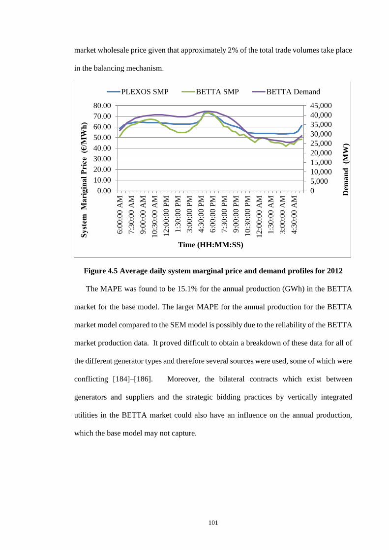
101

market wholesale price given that approximately 2% of the total trade volumes take place

in the balancing mechanism.

Figure 4.5 Average daily system marginal price and demand profiles for 2012

The MAPE was found to be 15.1% for the annual production (GWh) in the BETTA

market for the base model. The larger MAPE for the annual production for the BETTA

market model compared to the SEM model is possibly due to the reliability of the BETTA

market production data. It proved difficult to obtain a breakdown of these data for all of

the different generator types and therefore several sources were used, some of which were

conflicting [184]–[186]. Moreover, the bilateral contracts which exist between

generators and suppliers and the strategic bidding practices by vertically integrated

utilities in the BETTA market could also have an influence on the annual production,

which the base model may not capture.

0

5,000

10,000

15,000

20,000

25,000

30,000

35,000

40,000

45,000

0.00

10.00

20.00

30.00

40.00

50.00

60.00

70.00

80.00

6:0

0:0

0 A

M

7:3

0:0

0 A

M

9:0

0:0

0 A

M

10:3

0:0

0 A

M

12:0

0:0

0 P

M

1:3

0:0

0 P

M

3:0

0:0

0 P

M

4:3

0:0

0 P

M

6:0

0:0

0 P

M

7:3

0:0

0 P

M

9:0

0:0

0 P

M

10:3

0:0

0 P

M

12:0

0:0

0 A

M

1:3

0:0

0 A

M

3:0

0:0

0 A

M

4:3

0:0

0 A

M

Dem

an

d

(MW

)

Syst

em

Mari

gin

al

Pri

ce

(€/M

Wh

)

Time (HH:MM:SS)

PLEXOS SMP BETTA SMP BETTA Demand

102

4.5 Summary

The development of the 2012 PLEXOS base model including the main input

assumptions such as the generation portfolio, system demand and cost input data is

presented in this chapter. A comparative validation analysis between the base model

outputs and the actual SEM and BETTA markets data in 2012 is conducted. The

validated base model in 2012 is used for the analyses presented in this thesis as it can

replicate the SEM and BETTA markets outcomes based on the validation results

presented in this chapter. The validated base model is used as a starting point from which

the 2020 PLEXOS I-SEM model is developed. The methodology implemented for the I-

SEM model is presented in the next chapter.

103

5 I-SEM MODEL

5.1 Introduction

This chapter presents the methodology implemented for the 2020 PLEXOS I-SEM

model, which aligns with step five of the research methodology in Section 1.4. The

validated 2012 PLEXOS base model from Chapter 4 was used as a starting point from

which the 2020 I-SEM model for the analysis in this thesis was developed. The validated

2012 base model was extended to 2020 given that detailed representative data were

available for that year. This provided some certainty regarding the model assumptions

and scenarios. The BETTA market design in the 2020 model was kept the same as in the

2012 model but with a projected generation portfolio for 2020. Two model scenarios are

considered; Business as Usual (BAU) and BAU+CAES containing a CAES plant as an

additional generator, which are setup in the I-SEM model. A number of model

sensitivities are also carried out. The following subsections describe the I-SEM model,

model assumptions, model scenarios, CAES plant representation and model sensitivities.

5.2 I-SEM model description

A number of modifications were applied to the validated 2012 PLEXOS base model

in order to reflect the I-SEM and BETTA markets in 2020. The validated base model

consists of a DA model only and was used as a starting point from which the 2020 I-SEM

DA and BM models were developed. A high level representation of the I-SEM in 2020

was developed in PLEXOS given that detailed projected generation portfolio capacity

and system demand data were available for that year. Consequently, this provides some

certainty regarding the model assumptions and scenarios. However, the I-SEM model

only includes a representation of the short term DA and BM markets given that limited

104

information is currently available for the ID market design and the forwards market is

considered long term. The DA and BM market models were created in the I-SEM model

and the interleave method implemented in PLEXOS. The interleave method is a technique

for linking the outputs of one model with another and has been used in a number of studies

[138], [187], [188]. The interleave method run mode is manually invoked in the I-SEM

model by the user and the DA and BM models pass information back and forth between

each other as shown in Figure 5.1. This includes the optimisation of the DA unit

commitment (DAUC) schedule of generators in the DA model (Di-1) and passing of this

information (DA model output (Di-1)) to the BM model (Di)and the generators end state

(BM model end state (Di)) to the DA model (Di+1) for the next day. This process continues

daily over the year in order to create a realistic market simulation.

Figure 5.1 I-SEM model with interleaved DA and BM models

The I-SEM model reads the input data such as system demand and wind power output

as shown in Figure 5.1. It simulates 365 individual daily optimisations at an hourly time

105

resolution (the proposed time resolution for the I-SEM design) while ensuring the

generation portfolio meets demand at least cost while taking into account the generators’

techno-economic parameters. The purpose of the DA model (Di-1) is the creation of a

DAUC schedule. The scheduling of the DA model (Di-1) is carried out stochastically

using the scenario-wise decomposition method in PLEXOS in order to account for the

uncertainty in system wind and demand.

The scenario-wise decomposition method (which is manually invoked in the I-SEM

model by the user) uses two stage stochastic optimisation and paths are decomposed into

discrete trajectories called scenarios which have discrete probabilities. The probabilities

are assigned to each scenario; similar paths are combined or unlikely paths are removed

and the probabilities are recalculated. An initial unit commitment scheduling decision is

performed in the first stage, after which a random event occurs affecting the outcome of

the first stage decision. A recourse or new decision can then be made in the second stage

that compensates for any suboptimal unit commitment decision in the first stage. The

approach taken by the I-SEM model is a single first stage decision and a collection of

recourse decisions defining which second stage decision should be taken in response to

each random event. Further details of the I-SEM model stochastic equations are shown

in Appendix A. The generators planned maintenance outage schedules are always known

in advance of the DAUC schedule and are included in the model. The generators’ forced

outages are omitted as they occur randomly without advanced knowledge and are

included in the BM model. The interconnector flows are optimised based on the price

differential between the I-SEM and BETTA. The BETTA market design in the 2020 I-

SEM model remains the same as in the validated 2012 base model but with a projected

generation portfolio for 2020.

106

The purpose of the BM model is to re-optimise the DAUC schedule from the DA

model by moving generators dispatch levels up and down. The generators dispatch levels

are subsequently altered based on their decremental and incremental bids in the form of

price quantity pairs in response to the actual outcome of probabilistic events such as

system wind and demand. The interconnector flows are fixed in the BM model based on

the optimised flows from the DA model; as such the BETTA market and its associated

generators are prevented from participating in balancing the I-SEM. This simplication

may lead to suboptimal flows based on the simulated SMPs for the I-SEM and BETTA

markets. However, limited information is currently available in relation to the Irish and

British TSOs counter trading abilities on the interconnectors in the I-SEM. Moreover,

considering the significant amount of variable generation which the TSOs will be required

to balance in each market in 2020, they may be unable and/or reluctant to trade the spare

flexible capacity for balancing over the interconnectors.

5.3 I-SEM model assumptions

5.3.1 Generation portfolio

The I-SEM model was populated with the individual generator techno-economic

parameters for new entrants and retirements which have signed agreements and

confirmed dates to connect to the AII power system over the next 10 years [7]. It is

assumed the I-SEM generation portfolio achieves Ireland’s 2020 RES-E target. For the

BETTA market, the Slow Progression scenario is adopted from National Grid [189]. The

Slow Progression scenario represents a generation portfolio which does not meet the UK

RES-E and emissions targets for 2020. This scenario is chosen given the uncertainty

which the UK faces in achieving its target and it is assumed to be representative of the

projected generation portfolio in 2020 derived from National Grid’s stakeholder

107

engagement programme [189]. A breakdown of the generator types for both the I-SEM

and BETTA markets in 2020 is shown in Table 5.1. It is assumed both peat and distillate

oil generation are still operating in the I-SEM in 2020 as per the TSOs generation capacity

projections for 2020 [7]. However, there is some uncertainty in terms of peat generation

participating in the I-SEM as the PSO levy which currently supports peat generation is

proposed to cease by 2020. The generation portfolio for the BETTA market remains the

same for all the model scenarios and sensitivities. The modifications to the I-SEM

generation portfolio are described further in Section 5.4.

Generator type I-SEM BETTA

Coal 1,331 13,652

Gas 5,282 32,337

Oil 592 951

Nuclear 0 8,980

Distillate Oil 764 0

Peat 346 0

Total (MW) 8,315 55,920

Table 5.1 2020 aggregated conventional generation portfolio capacity (MW)

(Source: [7][189])

The renewable generation portfolio for the 2020 I-SEM and BETTA markets is shown

in Table 5.2. Similar to the 2012 base model, onshore and offshore wind provides the

predominant share of the renewable generation portfolio in both markets. Tidal

generation (assumed to be installed in NI) is the only new source of renewable generation

compared to the 2012 base model and it is assigned a 20% annual capacity factor from

Eirgrid and SONI [7] in the I-SEM model. The modelling approach for remaining

renewable generation is the same as in 2012 base model except for wind generation which

is described further in Section 5.3.2.

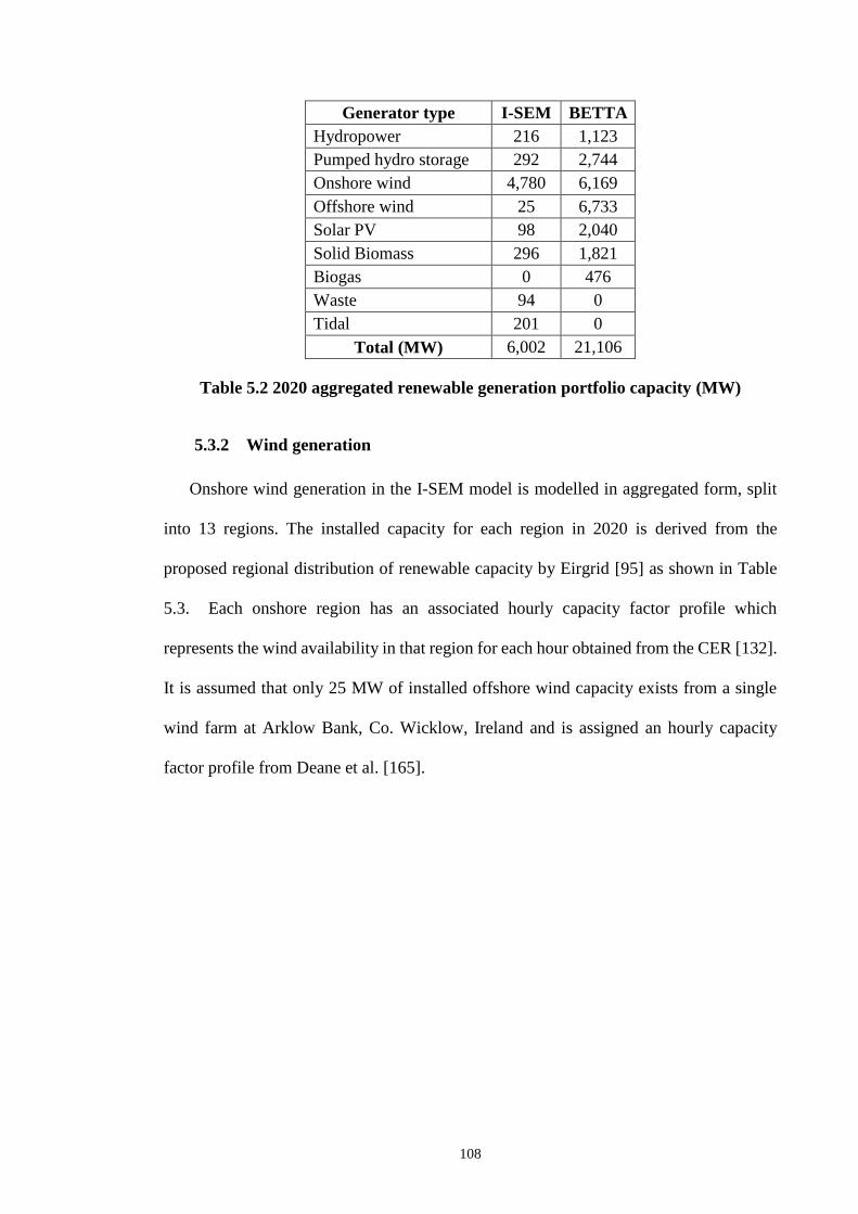
108

Generator type I-SEM BETTA

Hydropower 216 1,123

Pumped hydro storage 292 2,744

Onshore wind 4,780 6,169

Offshore wind 25 6,733

Solar PV 98 2,040

Solid Biomass 296 1,821

Biogas 0 476

Waste 94 0

Tidal 201 0

Total (MW) 6,002 21,106

Table 5.2 2020 aggregated renewable generation portfolio capacity (MW)

5.3.2 Wind generation

Onshore wind generation in the I-SEM model is modelled in aggregated form, split

into 13 regions. The installed capacity for each region in 2020 is derived from the

proposed regional distribution of renewable capacity by Eirgrid [95] as shown in Table

5.3. Each onshore region has an associated hourly capacity factor profile which

represents the wind availability in that region for each hour obtained from the CER [132].

It is assumed that only 25 MW of installed offshore wind capacity exists from a single

wind farm at Arklow Bank, Co. Wicklow, Ireland and is assigned an hourly capacity

factor profile from Deane et al. [165].

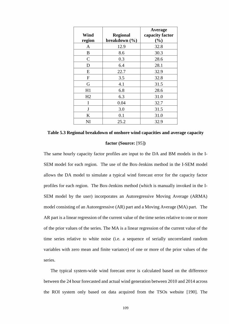
109

Wind

region

Regional

breakdown (%)

Average

capacity factor

(%)

A 12.9 32.8

B 8.6 30.3

C 0.3 28.6

D 6.4 28.1

E 22.7 32.9

F 3.5 32.8

G 4.1 31.5

H1 6.8 28.6

H2 6.3 31.0

I 0.04 32.7

J 3.0 31.5

K 0.1 31.0

NI 25.2 32.9

Table 5.3 Regional breakdown of onshore wind capacities and average capacity

factor (Source: [95])

The same hourly capacity factor profiles are input to the DA and BM models in the I-

SEM model for each region. The use of the Box-Jenkins method in the I-SEM model

allows the DA model to simulate a typical wind forecast error for the capacity factor

profiles for each region. The Box-Jenkins method (which is manually invoked in the I-

SEM model by the user) incorporates an Autoregressive Moving Average (ARMA)

model consisting of an Autoregressive (AR) part and a Moving Average (MA) part. The

AR part is a linear regression of the current value of the time series relative to one or more

of the prior values of the series. The MA is a linear regression of the current value of the

time series relative to white noise (i.e. a sequence of serially uncorrelated random

variables with zero mean and finite variance) of one or more of the prior values of the

series.

The typical system-wide wind forecast error is calculated based on the difference

between the 24 hour forecasted and actual wind generation between 2010 and 2014 across

the ROI system only based on data acquired from the TSOs website [190]. The

110

Normalised Mean Absolute Percentage Error (NMAPE) and Mean Absolute Error (MAE)

for ROI wind only between 2010 and 2014 are shown in Table 5.4. A normalised

NMAPE and MAE of 5.4% and 87 MW were calculated for the typical wind forecast

error, respectively. The statistical control parameters (α, β and σz) associated with the

typical wind forecast error growth and distribution are derived using an ARMA model in

statistical software package R [191]. The statistical control parameters are then used by

the ARMA model in the DA model to randomly generate the typical wind forecast error

for the capacity factor profiles for each region.

Year

NMAPE

(%)

MAE

(MW)

2010 5.66 76

2011 6.29 94

2012 5.36 87

2013 5.30 90

2014 4.47 90

Table 5.4 Annual wind forecast errors for the ROI

The onshore and offshore wind resource for the BETTA market model is represented

by hourly capacity factor profiles for the GB region taken from Deane et al. [165]. The

BETTA market model creates a DAUC schedule based on perfect foresight for all

variable renewable generation with no design or rules changes to the BETTA market. The

schedule is not re-optimised in the BM model timeframe and remains fixed during this

timeframe; therefore it is not contributing to balancing the I-SEM.

The 2020 I-SEM and BETTA market models are essentially unconstrained energy

only models. However, a main constraint restricting the amount of non-synchronous

generation, mainly wind, participating in the I-SEM and BETTA markets is enforced in

the models. This prevents wind contributing 100% to instantaneous demand and

therefore, replicates real conditions. The main constraint is known as the System Non-

111

Synchronous Penetration (SNSP) limit and is a measure of the non-synchronous

generation at an instant in time as shown by Equation 5.1 [89].

SPSNExportsDemand System

ImportsGeneration Wind

(5.1)

The SNSP limit ensures that the amount of wind generation, when added to

interconnector imports, does not exceed the sum of system demand and interconnector

exports. The TSOs in Ireland aim to increase the current SNSP limit of 50% up to 75%

by 2020, while empirical evidence from energy industry sources suggests that the

equivalent SNSP limit in GB will remain at approximately 50%. Therefore, the SNSP

limit is assumed to be 75% and 50% for the I-SEM and BETTA markets model in 2020,

respectively.

5.3.3 Maintenance schedules

Similar to the 2012 base model, the planned and unplanned maintenance outage

schedules for each generator during the year are taken into account in the 2020 I-SEM

and BETTA models. For the I-SEM model, the generators planned maintenance outage

schedules are always known in advance of the DAUC schedule and are included in the

DA model. The generators’ unplanned maintenance represented by forced outage rates

and mean time to repair from CER [132] are omitted in the DA model as they occur

randomly without advanced knowledge and are included in the BM model. For the

BETTA model, maintenance outage schedules for each generator are modelled as a

random event based on the forced outage rates and mean time to repair values from the

2012 base model.

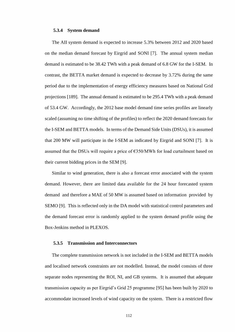
112

5.3.4 System demand

The AII system demand is expected to increase 5.3% between 2012 and 2020 based

on the median demand forecast by Eirgrid and SONI [7]. The annual system median

demand is estimated to be 38.42 TWh with a peak demand of 6.8 GW for the I-SEM. In

contrast, the BETTA market demand is expected to decrease by 3.72% during the same

period due to the implementation of energy efficiency measures based on National Grid

projections [189]. The annual demand is estimated to be 295.4 TWh with a peak demand

of 53.4 GW. Accordingly, the 2012 base model demand time series profiles are linearly

scaled (assuming no time shifting of the profiles) to reflect the 2020 demand forecasts for

the I-SEM and BETTA models. In terms of the Demand Side Units (DSUs), it is assumed

that 200 MW will participate in the I-SEM as indicated by Eirgrid and SONI [7]. It is

assumed that the DSUs will require a price of €350/MWh for load curtailment based on

their current bidding prices in the SEM [9].

Similar to wind generation, there is also a forecast error associated with the system

demand. However, there are limited data available for the 24 hour forecasted system

demand and therefore a MAE of 50 MW is assumed based on information provided by

SEMO [9]. This is reflected only in the DA model with statistical control parameters and

the demand forecast error is randomly applied to the system demand profile using the

Box-Jenkins method in PLEXOS.

5.3.5 Transmission and Interconnectors

The complete transmission network is not included in the I-SEM and BETTA models

and localised network constraints are not modelled. Instead, the model consists of three

separate nodes representing the ROI, NI, and GB systems. It is assumed that adequate

transmission capacity as per Eirgrid’s Grid 25 programme [95] has been built by 2020 to

accommodate increased levels of wind capacity on the system. There is a restricted flow

113

of 450 MW in the NI-ROI and 400 MW ROI-NI directions at present due to system

security issues. However, the full rating of the North-South transmission line between NI

and ROI is assumed to be in place by 2020; therefore flows of 1500 MW both ways are

set within the model [192].

There are a number of new interconnectors due to come online between 2012 and

2020. The East-West interconnector between the I-SEM and BETTA markets is added

to the I-SEM model, a maximum flow of 500 MW was assumed both ways. The proposed

IFA2 interconnector between the BETTA and French markets is included in the model

with a maximum flow of 1,000 MW both ways [193]. The existing interconnectors

(Moyle, BritNed and IFA) which were in the 2012 base model retain the same capacity

and are also included in the I-SEM model. The interconnector flows between the I-SEM

and BETTA markets are allowed to be freely optimised in the DA model but are fixed in

the BM model. The import and export flows for the interconnectors from mainland

Europe to the BETTA market are fixed in both the DA and BM models based on flows

obtained from Cleary et al. [142]. Similar to the 2012 base model, this simplified

approach was adopted as it reduces the need to create a detailed representation of the

Dutch and French markets and significantly reduces computational time.

5.3.6 Cost Input data

Fuel prices from the 2012 base model in Chapter 4 are adjusted based on predictions

for 2020 from DECC [194] and inputted to the I-SEM and BETTA models. It is

acknowledged that fuel prices have fluctuated since these predictions and they will have

an impact on the simulated outputs for this analysis. Therefore, in order to show the

impact of changes in the fuel prices a sensitivity analysis is conducted and is described

further in Section 5.7.

114

A carbon price of €30/t CO2 based on the European Union ETS was applied to fossil

fuel-based generators in the I-SEM model. This figure is based on the carbon taxes used

for previous Irish case studies, which ranged between €15-45/t CO2 [121], [175], [176],

[195], [196]. A carbon price of €34/t CO2 based on the Carbon Price Floor (CPF) was

applied to fossil fuel-based generators in the BETTA model [77]. Generator VOM and

start costs are adjusted accordingly and all cost data were normalised to 2012 values using

historic consumer price indices [177].

5.4 Model scenarios

This section presents the I-SEM model scenarios incorporated in each I-SEM model

simulation, which forms step six of the research methodology in Section 1.4. Two main

operational scenarios in the 2020 I-SEM model are considered; Business as Usual (BAU)

and BAU+CAES containing a CAES plant as an additional generator in the I-SEM. The

generation portfolio for the BETTA market model remains the same for each model

scenario. A description of each scenario is as follows:

1. BAU represents the 2020 I-SEM with a generation portfolio as shown previously

in Table 5.1 and Table 5.2 in Section 5.3.1. This scenario is considered to

represent the I-SEM generation portfolio in 2020 given the new entrants and

retirements planned over the next 10 years for the AII power system [7] [164].

The modelling approach presented in the previous sections replicates the proposed

I-SEM rules and hence, this scenario is considered to represent a simple but

realistic real-time energy only operation of the I-SEM.

2. BAU+CAES is the BAU scenario with a CAES plant included in the 2020 I-SEM

generation portfolio. This scenario is considered to represent a proposed 2020 I-

SEM generation portfolio given the potential which exists for a CAES plant to be

connected to the AII power system [23].

115

5.5 CAES plant representation

A CAES plant is represented in the I-SEM model for the BAU+CAES scenario only

by a PHES plant coupled with a conventional gas plant using constraints to replicate the

operation of the plant as shown in Figure 5.2. This approximation of the CAES plant

configuration was used previously for other case studies [20], [133], [197].

Figure 5.2 CAES plant configuration in 2020 I-SEM model

In compression mode (as shown by the red dashed line in Figure 5.2) the Pumped

Storage Pump draws power from the electricity grid within the I-SEM model to compress

air to Storage, while in generation mode (as shown by the blue dashed line in Figure 5.2)

both the Pump Storage Generator and Gas Generator provide electricity back to the grid.

A constraint limiting the combined output of the Pump Storage Generator and Gas

Generator is set based on the maximum generation capacity of the CAES plant. The

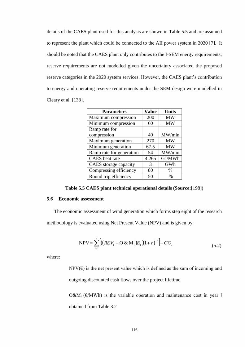
116

details of the CAES plant used for this analysis are shown in Table 5.5 and are assumed

to represent the plant which could be connected to the AII power system in 2020 [7]. It

should be noted that the CAES plant only contributes to the I-SEM energy requirements;

reserve requirements are not modelled given the uncertainty associated the proposed

reserve categories in the 2020 system services. However, the CAES plant’s contribution

to energy and operating reserve requirements under the SEM design were modelled in

Cleary et al. [133].

Parameters Value Units

Maximum compression 200 MW

Minimum compression 60 MW

Ramp rate for

compression 40 MW/min

Maximum generation 270 MW

Minimum generation 67.5 MW

Ramp rate for generation 54 MW/min

CAES heat rate 4.265 GJ/MWh

CAES storage capacity 3 GWh

Compressing efficiency 80 %

Round trip efficiency 50 %

Table 5.5 CAES plant technical operational details (Source:[198])

5.6 Economic assessment

The economic assessment of wind generation which forms step eight of the research

methodology is evaluated using Net Present Value (NPV) and is given by:

(5.2)

where:

NPV(€) is the net present value which is defined as the sum of incoming and

outgoing discounted cash flows over the project lifetime

O&Mi (€/MWh) is the variable operation and maintenance cost in year i

obtained from Table 3.2

0

n

1i

i 1M&O= NPV CCrEREVi

ii

117

CC0 (€/MW) is the capital cost in year 0 obtained from Table 3.2 for the 2012

project and multiplied by the onshore wind capacity from Table 5.2

Ei is the electricity produced in BM in year i (MWh) obtained from the I-SEM

model

r is the WACC (%) obtained from Table 3.2

n is the lifespan (years) obtained from Table 3.2

REVi (€/MWh) is the revenue wind generation earns in year i in the I-SEM

based on the SMPs simulated by the I-SEM model.

REVi = Q1 x P1 + (Q0-Q1) x P0 (5.3)

where:

Q0 (MWh) is the BM wind production

Q1 (MWh) is the DA wind production

P0 (€/MWh) is the BM price

P1(€/MWh) is the DA price

5.7 Model sensitivities

A sensitivity analysis is undertaken in order to determine how sensitive the main I-

SEM model outputs such as the system marginal prices, total generation costs and CO2

emissions are to the underlying model input assumptions, including system demand and

wind forecast errors, fuel and carbon prices as well as generators decremental and

incremental bids. A low and high sensitivity analysis is carried out for both BAU and

BAU+CAES scenarios, which examines the effects of changes in the underlying model

input assumptions. The key sensitivity input parameters assessed for the I-SEM model

118

are the changes in the wind and demand forecast error, generators increments (incs) and

decrements (decs) and the fuel and carbon prices given the uncertainty associated with

these parameters. In particular, fuel prices can be can be extremely unpredictable and

volatile due to geopolitical issues and supply concerns. It should be noted that the CAES

plant and wind generation capital costs were not considered as part of the sensitivity

analysis given they are not input parameters to the I-SEM model. However, the selected

key sensitivity input parameters will impact both the CAES plant and wind generation.

The wind and demand forecast errors are described in Sections 5.3.2 and 5.3.4 and

are represented by the NMAPE and MAE. The forecasted and actual wind generation

between 2010 and 2014 based on data acquired from the TSOs website (as described in

Section 5.3.2) is analysed and used as a basis for the improvement and deterioration of

the wind forecast error. There is limited data available for the system demand, therefore

the same improvement and deterioration for the wind forecast error is applied to the

demand forecast error. Based on improved wind and demand forecast errors relative to

the initial input parameters (defined as central) in the I-SEM model, the low sensitivity

input parameters are set at a MAE of 44 MW and 25 MW assuming the forecast improves

by 50%, respectively. Based on less accurate wind and demand forecast errors relative to

the base case, the high sensitivity input parameters are set at a MAE of 118 MW and 75

MW assuming the forecast deteriorates by 50%, respectively.

The generators incs and decs are more difficult to estimate as they are dependent on

the real time status of the BM market and the strategic bidding behaviour of generators at

that point in time. For instance, if the BM market timeframe is short (i.e. the system

requires additional generation or reduction in demand), generators will need to increase

generation and therefore will require additional remuneration, while if the BM is long

(i.e. the system requires a reduction in generation or increase in demand), generators will

119

generally accept their original DA Short Run Marginal Cost (SRMC) bid. The low and

high sensitivity input parameters for generators incs and decs categorised under baseload,

mid-merit and peaker based on a review of literature and industry engagement is shown

in Table 5.6. It is assumed that generators will take the DA SRMC bid as the dec price

for both low and high sensitivities. If the generator is on or off it will require the SRMC

plus a certain mark-up for the inc price.

The I-SEM model central input parameters for fuel and carbon prices were outlined

earlier in Section 5.3.6. The low and high fuel price sensitivity input parameters are

shown in Table 5.7 and are set based on the DECC [77] low and high fuel price projections

for 2020. A carbon price of €15/t CO2 and €45/t CO2 is set for the low and high carbon

price sensitivity input parameters, respectively. These figures are based on the carbon

taxes used for previous Irish case studies, which ranged between €15-45/t CO2 [121],

[175], [176], [195], [196].

120

Sensitivity

Low Central High

Generator

category Baseload Mid-merit Peaker Baseload Mid-merit Peaker Baseload Mid-merit Peaker

Decrement

price SRMC x 1 SRMC x 1 SRMC x 1 SRMC x 1 SRMC x 1 SRMC x 1 SRMC x 1 SRMC x 1 SRMC x 1

Increment

price

(when

plant on) SRMC x 1 SRMC x 1 SRMC x 1

SRMC x

1.05

SRMC x

1.05

SRMC x

1.05

SRMC x

1.1

SRMC x

1.1

SRMC x

1.1

Increment

price

(when

plant off) No offer No offer

SRMC x

1.05 No offer No offer

SRMC x

1.1 No offer No offer

SRMC x

1.15

Table 5.6 Low, central and high sensitivity input parameters for decrement and increment prices

121

Sensitivity

Low Central High

Fuel price (€/GJ)

Fuel type Q1

2020

Q2

2020

Q3

2020

Q4

2020

Q1

2020

Q2

2020

Q3

2020

Q4

2020

Q1

2020

Q2

2020

Q3

2020

Q4

2020

NI Gas 5.24 5.09 5.09 5.58 9.19 8.92 8.93 9.78 11.76 11.41 11.43 12.52

RoI Gas 5.22 5.06 5.06 5.56 9.16 8.87 8.88 9.75 11.72 11.35 11.37 12.48

NI Oil 13.01 12.17 12.64 11.65 18.06 16.90 17.55 16.18 19.72 20.28 21.06 19.42

RoI Oil 13.27 12.43 12.90 11.91 18.43 17.27 17.92 16.54 20.12 20.72 21.50 19.85

NI Coal 3.76 3.48 3.51 3.44 4.95 4.57 4.63 4.53 5.54 5.13 5.18 5.07

RoI Coal 3.32 3.02 3.06 2.98 4.37 3.97 4.03 3.92 4.89 4.45 4.51 4.39

NI

Distillate 16.35 16.07 16.56 15.50 22.71 22.32 22.99 21.52 27.26 26.79 27.59 25.83

RoI

Distillate 16.62 16.34 16.82 15.77 23.09 22.70 23.36 21.90 27.71 27.24 28.03 26.28

Table 5.7 Low, central and high sensitivity input parameters for fuel prices

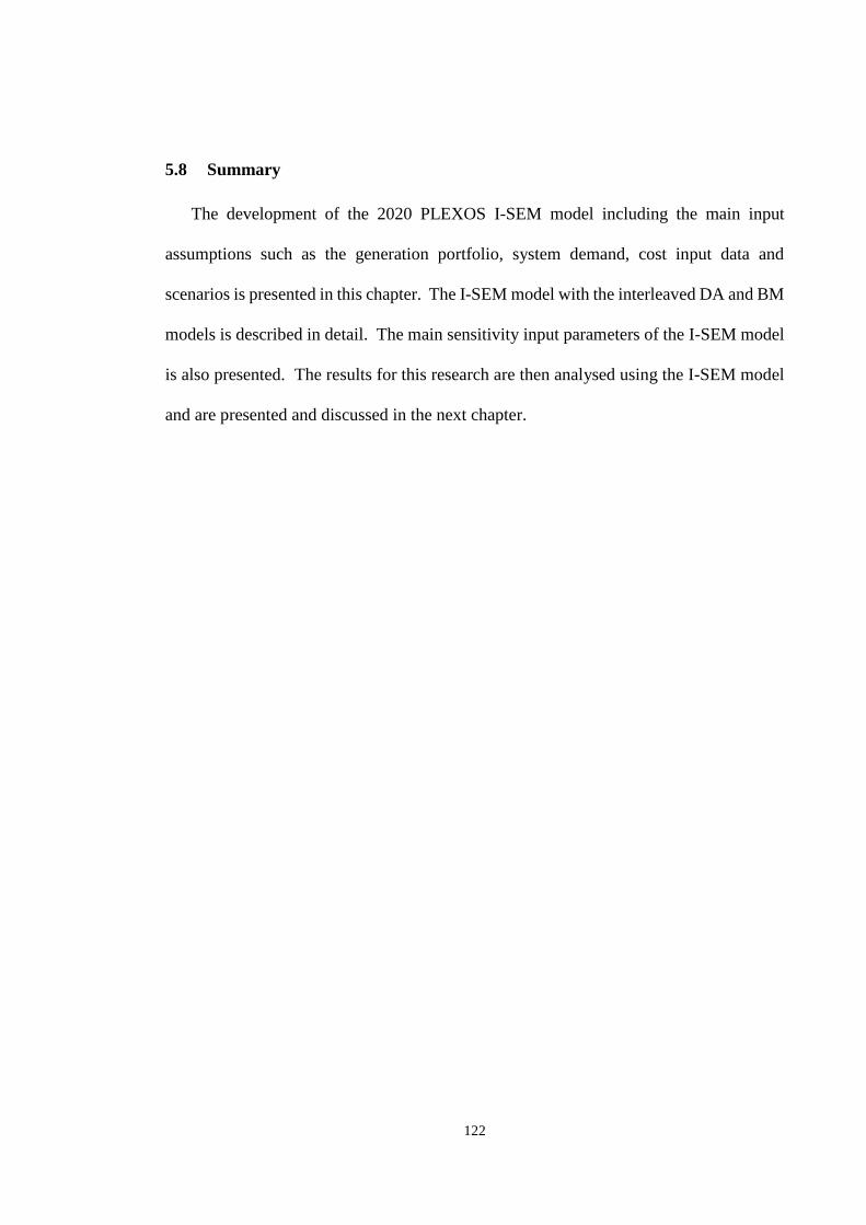
122

5.8 Summary

The development of the 2020 PLEXOS I-SEM model including the main input

assumptions such as the generation portfolio, system demand, cost input data and

scenarios is presented in this chapter. The I-SEM model with the interleaved DA and BM

models is described in detail. The main sensitivity input parameters of the I-SEM model

is also presented. The results for this research are then analysed using the I-SEM model

and are presented and discussed in the next chapter.

123

6 RESULTS AND DISCUSSION

6.1 Introduction

This chapter presents and discusses the main results for this research, which aligns

with the specific research objectives as outlined in Section 1.3. The 2020 I-SEM model

described in Chapter 5 was used to simulate the main results presented in this chapter.

Two model scenario results are presented; Business as Usual (BAU) and BAU+CAES

containing a CAES plant as an additional generator in the I-SEM. The generation output

mix, wind curtailment, system marginal prices, total generation costs and CO2 emissions

are initially presented and discussed. The NPV of wind generation is then assessed using

cost data from Chapter 3 as well as SMP and generation outputs from the I-SEM model

for each scenario. An economic assessment of the CAES plant from systems perspective

is also presented. Finally, sensitivity analysis results for the key I-SEM model input

parameters are presented. The following sections present and discuss the results in more

detail.

6.2 Generation output mix

The I-SEM model estimates of generation output mix for the BAU and BAU+CAES

scenarios are shown in Table 6.1. Gas generation dominates both scenarios, with peat,

other renewables (i.e. biomass and tidal) and wind representing important portions of the

generation output mix. In both scenarios, there is a decrease in wind generation between

the DA and BM markets resulting in increased utilisation of generation mainly from coal,

gas and distillate oil. This increase is primarily due to the increased utilisation of fast

acting generation, in particular gas and distillate oil responding to a 1.9% decrease

(decreasing from 13,582 GWh to 13,333 GWh as shown in Table 6.1) in wind generation.

The introduction of the CAES plant in the BAU+CAES scenario alters the generation

output mix relative to the BAU scenario resulting in increased use of coal generation and

124

decreased use of gas generation and interconnection imports from the BETTA market.

The CAES plant has a generation output of 743 GWh in the BM market displacing the

less flexible and more expensive gas generators. Moreover, the CAES plant increases

system demand while in compression mode, typically during off peak and coal generation

which is generally in merit during these hours, responses to the increase in demand.

Table 6.1 Generation comparison for BAU and BAU+CAES scenarios

6.3 Wind curtailment

The SNSP limit as described in Section 2.1.4 and Section 5.3.2 is imposed by the

TSOs to ensure security of supply and stable voltage and frequency on the power system.

Therefore, with increased levels of wind generation comes the possibility of increased

curtailment of wind generators, such as during high wind generation periods coinciding

with low system demand. Curtailment of wind generators can result in loss of revenue for

wind farm operators. The wind curtailment levels were found to decrease slightly from

1.35% to 1.23% between the BAU and BAU+CAES scenarios, respectively. For

instance, when a curtailment event occurs in the BAU+CAES scenario with a 75% SNSP

limit, for each 100 MW of increased demand created by the CAES plant in compression

mode, it allows 75 MW of wind to remain connected and increases the synchronous

generation by 25 MW to satisfy the SNSP limit.

Generator Type Day-Ahead Balancing

MechanismDifference Day-Ahead

Balancing

MechanismDifference

Coal 431 465 34 622 638 16

Gas 21,310 21,726 416 21,102 21,567 465

Peat 2,172 2,075 -97 2,117 2,026 -90

Distillate oil 0 132 132 0 126 126

Hydro 747 727 -20 743 723 -20

Pumped hydro storage 314 299 -14 260 248 -11

CAES - - - 697 743 46

Wind 13,582 13,333 -249 13,583 13,349 -234

Other renewables 3,749 3,696 -54 3,756 3,702 -55

Interconnection Imports 722 722 0 551 551 0

Interconnection Exports 2844 2844 0 2799 2799 0

Net Total (GWh) 43,027 43,174 147 43,431 43,673 243

BAU Generation (GWh) BAU+CAES Generation (GWh)

125

6.4 System Marginal Prices

A comparison of the simulated annual average wholesale System Marginal Prices

(SMPs) for the DA and BM markets for each scenario are shown in Figure 6.1. It can be

seen that the SMP increases from €80.46/MWh to €124/MWh between the DA and BM

markets for the BAU scenario. This increase is primarily due to the increased utilisation

of fast acting generation, in particular gas and distillate oil (which have higher costs

because they are generally operating either at part load or from start-up) responding to

the decrease in wind generation as highlighted in Section 6.2. Similarly, the SMP

increases from €80.96/MWh to €125.31/MWh between the DA and BM markets in the

BAU+CAES scenario, where wind generation decreases 1.8% (decreasing from 13,583

GWh to 13,349 GWh as shown in Table 6.1), with the more costly generators ramping

and/or starting up to meet the deficit in generation. While there is minor decrease in the

system demand between the DA and BM markets for both scenarios, it has a negligible

effect on the generation output mix and SMPs. Moreover, it should be noted that the

estimated SMPs are highly sensitive to the underlying assumptions including the fuel and

carbon prices, generators decremental and incremental bids. A number of sensitivities

are carried out in Section 6.9 which examines the effects of changes in the underlying

assumptions on the key output parameters.

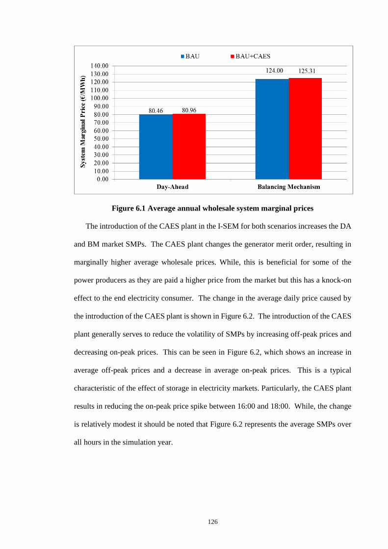
126

Figure 6.1 Average annual wholesale system marginal prices

The introduction of the CAES plant in the I-SEM for both scenarios increases the DA

and BM market SMPs. The CAES plant changes the generator merit order, resulting in

marginally higher average wholesale prices. While, this is beneficial for some of the

power producers as they are paid a higher price from the market but this has a knock-on

effect to the end electricity consumer. The change in the average daily price caused by

the introduction of the CAES plant is shown in Figure 6.2. The introduction of the CAES

plant generally serves to reduce the volatility of SMPs by increasing off-peak prices and

decreasing on-peak prices. This can be seen in Figure 6.2, which shows an increase in

average off-peak prices and a decrease in average on-peak prices. This is a typical

characteristic of the effect of storage in electricity markets. Particularly, the CAES plant

results in reducing the on-peak price spike between 16:00 and 18:00. While, the change

is relatively modest it should be noted that Figure 6.2 represents the average SMPs over

all hours in the simulation year.

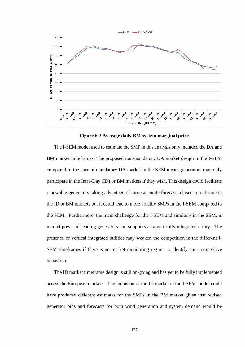
127

Figure 6.2 Average daily BM system marginal price

The I-SEM model used to estimate the SMP in this analysis only included the DA and

BM market timeframes. The proposed non-mandatory DA market design in the I-SEM

compared to the current mandatory DA market in the SEM means generators may only

participate in the Intra-Day (ID) or BM markets if they wish. This design could facilitate

renewable generators taking advantage of more accurate forecasts closer to real-time in

the ID or BM markets but it could lead to more volatile SMPs in the I-SEM compared to

the SEM. Furthermore, the main challenge for the I-SEM and similarly in the SEM, is

market power of leading generators and suppliers as a vertically integrated utility. The

presence of vertical integrated utilities may weaken the competition in the different I-

SEM timeframes if there is no market monitoring regime to identify anti-competitive

behaviour.

The ID market timeframe design is still on-going and has yet to be fully implemented

across the European markets. The inclusion of the ID market in the I-SEM model could

have produced different estimates for the SMPs in the BM market given that revised

generator bids and forecasts for both wind generation and system demand would be

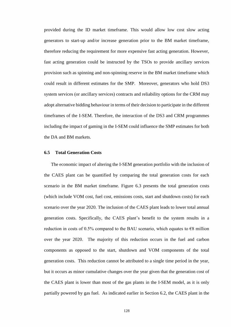
128

provided during the ID market timeframe. This would allow low cost slow acting

generators to start-up and/or increase generation prior to the BM market timeframe,

therefore reducing the requirement for more expensive fast acting generation. However,

fast acting generation could be instructed by the TSOs to provide ancillary services

provision such as spinning and non-spinning reserve in the BM market timeframe which

could result in different estimates for the SMP. Moreover, generators who hold DS3

system services (or ancillary services) contracts and reliability options for the CRM may

adopt alternative bidding behaviour in terms of their decision to participate in the different

timeframes of the I-SEM. Therefore, the interaction of the DS3 and CRM programmes

including the impact of gaming in the I-SEM could influence the SMP estimates for both

the DA and BM markets.

6.5 Total Generation Costs

The economic impact of altering the I-SEM generation portfolio with the inclusion of

the CAES plant can be quantified by comparing the total generation costs for each

scenario in the BM market timeframe. Figure 6.3 presents the total generation costs

(which include VOM cost, fuel cost, emissions costs, start and shutdown costs) for each

scenario over the year 2020. The inclusion of the CAES plant leads to lower total annual

generation costs. Specifically, the CAES plant’s benefit to the system results in a

reduction in costs of 0.5% compared to the BAU scenario, which equates to €8 million

over the year 2020. The majority of this reduction occurs in the fuel and carbon

components as opposed to the start, shutdown and VOM components of the total

generation costs. This reduction cannot be attributed to a single time period in the year,

but it occurs as minor cumulative changes over the year given that the generation cost of

the CAES plant is lower than most of the gas plants in the I-SEM model, as it is only

partially powered by gas fuel. As indicated earlier in Section 6.2, the CAES plant in the

129

BAU+CAES scenario alters the generation output mix relative to the BAU scenario, in

particular resulting in decreased use of gas generation. From a technical perspective, this

reduction is due to the CAES plant’s ability in providing additional flexibility, as the plant

has no minimum up/down times and has larger ramp rates relative to the gas plants.

Therefore, the I-SEM model takes advantage of the CAES plant’s lower generation cost

and flexibility by displacing the more expensive and less flexible generation.

Figure 6.3 Total generation costs for each model scenario

6.6 CO2 emissions

Carbon dioxide (CO2) emissions were estimated for each generator type for each

scenario in the BM market timeframe and are presented in aggregated form in Figure 6.4.

The quantity of CO2 emissions generated is a function of the amount of carbon in the fuel

and the quantity of fuel burnt by each generator type. It can be seen there is a modest

emissions increase of 1% (0.1 MtCO2) between the BAU and BAU+CAES scenarios due

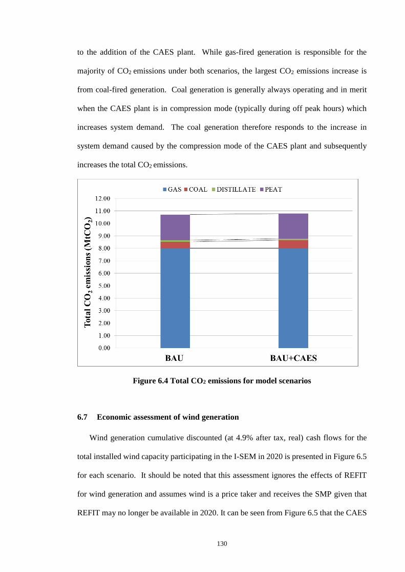
130

to the addition of the CAES plant. While gas-fired generation is responsible for the

majority of CO2 emissions under both scenarios, the largest CO2 emissions increase is

from coal-fired generation. Coal generation is generally always operating and in merit

when the CAES plant is in compression mode (typically during off peak hours) which

increases system demand. The coal generation therefore responds to the increase in

system demand caused by the compression mode of the CAES plant and subsequently

increases the total CO2 emissions.

Figure 6.4 Total CO2 emissions for model scenarios

6.7 Economic assessment of wind generation

Wind generation cumulative discounted (at 4.9% after tax, real) cash flows for the

total installed wind capacity participating in the I-SEM in 2020 is presented in Figure 6.5

for each scenario. It should be noted that this assessment ignores the effects of REFIT

for wind generation and assumes wind is a price taker and receives the SMP given that

REFIT may no longer be available in 2020. It can be seen from Figure 6.5 that the CAES

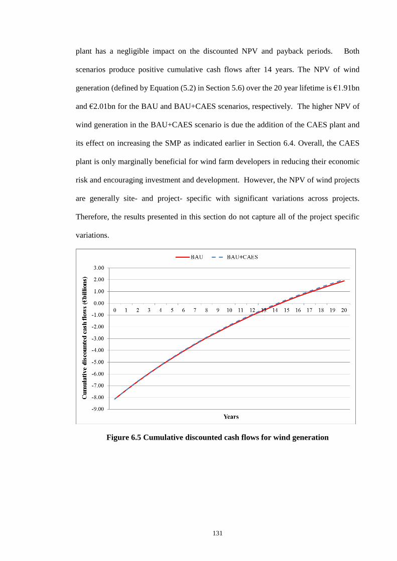
131

plant has a negligible impact on the discounted NPV and payback periods. Both

scenarios produce positive cumulative cash flows after 14 years. The NPV of wind

generation (defined by Equation (5.2) in Section 5.6) over the 20 year lifetime is €1.91bn

and €2.01bn for the BAU and BAU+CAES scenarios, respectively. The higher NPV of

wind generation in the BAU+CAES scenario is due the addition of the CAES plant and

its effect on increasing the SMP as indicated earlier in Section 6.4. Overall, the CAES

plant is only marginally beneficial for wind farm developers in reducing their economic

risk and encouraging investment and development. However, the NPV of wind projects

are generally site- and project- specific with significant variations across projects.

Therefore, the results presented in this section do not capture all of the project specific

variations.

Figure 6.5 Cumulative discounted cash flows for wind generation

132

6.8 Evaluation of CAES

In this section the evaluation of the CAES plant in terms of whether investment in

such a technology is economically viable from a systems perspective is presented. Table

6.2 presents the total generation cost, compression cost, pool revenue and net revenue

(the revenue collected in the energy market minus the total generation cost and

compression cost) for the CAES plant over the year 2020. While additional revenues for

the CAES plant include reserve revenue from the DS3 system services and annual

capacity payments from the CRM, this analysis has not taken these additional revenues

into account. This is due to the uncertainty of how CAES will participate in the different

I-SEM timeframes and whether it receives a DS3 system services contract and holds

reliability options for the CRM. Furthermore, the DS3 and CRM programmes are

currently under regulatory and stakeholder consultation and it is difficult to determine

what these programmes may offer a CAES plant investor.

The sole revenue stream for the CAES plant considered here is from electricity price

arbitrage (i.e. the plant is in compression mode when the electricity price is low and

generates during periods of high electricity price). However, it be should noted that this

could under estimate the economics of the CAES plant given that this assessment ignores

the additional revenue streams outlined above. Table 6.2 presents the total generation

cost (including VOM cost, fuel cost and emissions costs); compression cost (product of

price charged in €/MWh and consumption in MWh); pool revenue (product of price

received in €/MWh and generation in MWh) and net revenue (the pool revenue minus the

total generation cost and compression cost) for the CAES plant. The CAES plant receives

positive net revenue of €21.6 million over the year 2020. From a system perspective, the

CAES plant recovers it costs from the revenue of selling energy to the I-SEM given that

133

the SMP incentives the on-going operation of the plant therefore it is considered

economically viable.

Moreover, based on a capital cost of €733/kW from Table 2.2 for the CAES plant and

annual net revenues of €21.6 million; the simple payback period is less than 10 years. The

typical lifetime of a CAES plant is 30 years and it would be a private investor’s decision

if the investment exposure period of 10 years is acceptable. However, a private NPV

analysis of the CAES plant is outside of the scope of this analysis given the uncertainty

of the DS3 system services and CRM payments to such a plant.

Item Value (€000)

Total generation cost 11,783

Compression cost 30,490

Pool revenue 63,898

Net Revenue 21,626

Table 6.2 CAES plant costs and revenues

6.9 Sensitivity analysis results

6.9.1 System marginal prices

The SMPs from the I-SEM model using the initial input parameters (defined as

central) for the DA and BM market timeframes were presented earlier in Section 6.4. The

BM market SMPs for the BAU and BAU+CAES scenarios were recalculated using the I-

SEM model with the low and high sensitivity input parameters as described in Section

5.7. Figure 6.6 and Figure 6.7 presents the SMPs for the low and high sensitivities for

the BAU and BAU+CAES scenarios. The simulated SMPs from the I-SEM model using

the initial input parameters (defined as central) are represented in both figures by the

vertical axis. It can be seen from Figure 6.6 and Figure 6.7 that the SMPs are most

sensitive to the fuel and carbon prices, while the remaining input parameters have a more

modest impact. The SMPs for the fuel prices decrease and increase for the low and high

sensitivities to €94.32/MWh (24% decrease) and €128.94/MWh (4% increase),

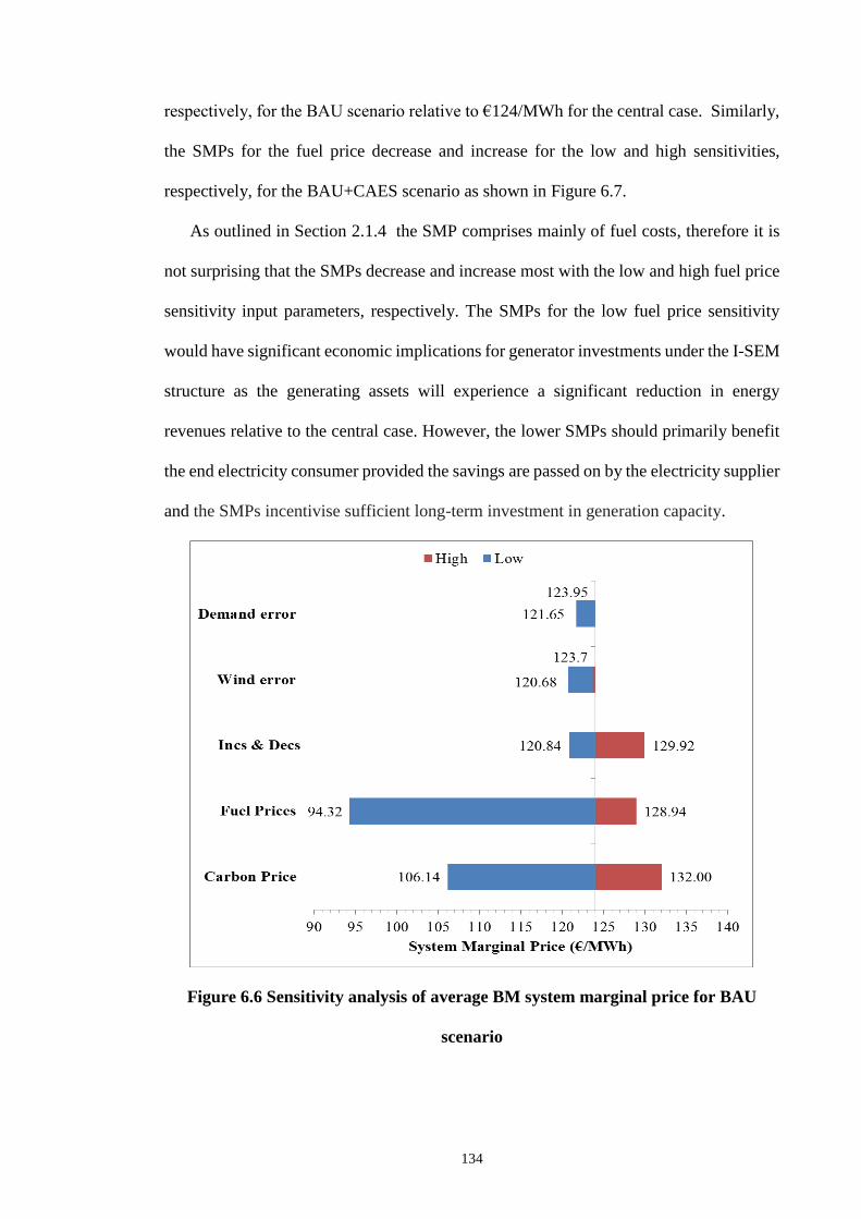
134

respectively, for the BAU scenario relative to €124/MWh for the central case. Similarly,

the SMPs for the fuel price decrease and increase for the low and high sensitivities,

respectively, for the BAU+CAES scenario as shown in Figure 6.7.

As outlined in Section 2.1.4 the SMP comprises mainly of fuel costs, therefore it is

not surprising that the SMPs decrease and increase most with the low and high fuel price

sensitivity input parameters, respectively. The SMPs for the low fuel price sensitivity

would have significant economic implications for generator investments under the I-SEM

structure as the generating assets will experience a significant reduction in energy

revenues relative to the central case. However, the lower SMPs should primarily benefit

the end electricity consumer provided the savings are passed on by the electricity supplier

and the SMPs incentivise sufficient long-term investment in generation capacity.

Figure 6.6 Sensitivity analysis of average BM system marginal price for BAU

scenario

135

Figure 6.7 Sensitivity analysis of average BM system marginal price for

BAU+CAES scenario

6.9.2 Total generation costs

The total generation costs for the I-SEM model using the initial input parameters were

presented earlier in Section 0. The changes in the total generation costs for the low and

high sensitivities for the BAU and BAU+CAES scenarios are shown in Figure 6.8 and

Figure 6.9. The generation costs are highly sensitive to the fuel price for both scenarios,

while the remaining input parameters have a modest impact on the costs. This is

reasonable given that the fuel costs make up a significant portion of the total generation

costs. It can be seen from Figure 6.8 that the generation costs for the fuel price decrease

for the low and high sensitivities to €1.403 billion (26% decrease) and €1.671 billion (6%

decrease), respectively, for the BAU scenario relative to €1.765 billion for the base case.

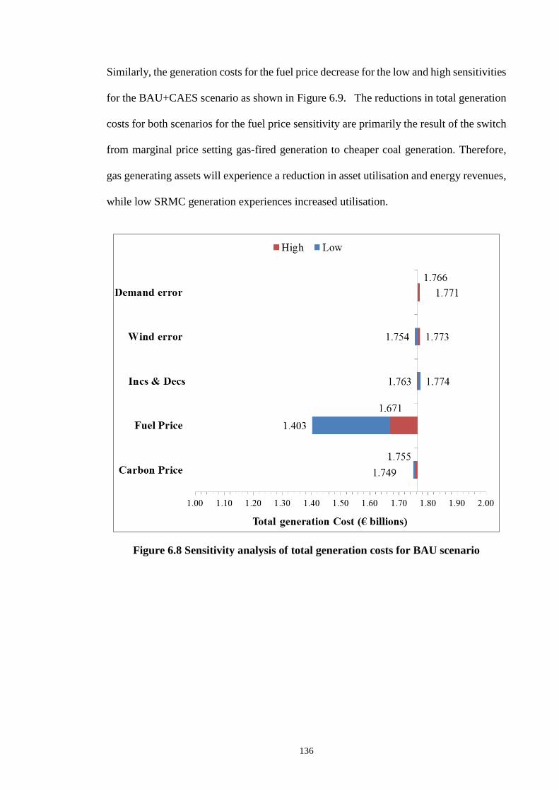
136

Similarly, the generation costs for the fuel price decrease for the low and high sensitivities

for the BAU+CAES scenario as shown in Figure 6.9. The reductions in total generation

costs for both scenarios for the fuel price sensitivity are primarily the result of the switch

from marginal price setting gas-fired generation to cheaper coal generation. Therefore,

gas generating assets will experience a reduction in asset utilisation and energy revenues,

while low SRMC generation experiences increased utilisation.

Figure 6.8 Sensitivity analysis of total generation costs for BAU scenario

137

Figure 6.9 Sensitivity analysis of total generation costs for BAU+CAES scenario

6.9.3 CO2 emissions

The CO2 emissions for the I-SEM model were presented in Section 0, while the

change in the CO2 emissions for the low and high sensitivities for the BAU and

BAU+CAES scenarios is shown in Figure 6.10 and Figure 6.11. The CO2 emissions are

highly sensitive to the carbon price for both scenarios, while their impacts on the

remaining input parameters have a modest effect on the emissions. This is reasonable

given that an increase in the carbon price should prevent carbon intensive generators from

being dispatched as their SRMC will increase and be out of merit. Moreover, this also

reduces the overall CO2 emissions if such carbon intensive generators are economically

constrained by the carbon price. It can be seen from Figure 6.10 that the emissions for

the carbon price increase and decrease for the low and high sensitivities to 14.65 MtCO2

(37% increase) and 8.87 MtCO2 (21% decrease), respectively, for the BAU scenario

relative to 10.71 MtCO2 for the central case. For the BAU+CAES scenario, the emissions

138

for the carbon price increase and decrease for the low and high sensitivities to 15.15

MtCO2 (40% increase) and 8.8 MtCO2 (23% decrease), respectively, relative to 10.79

MtCO2 for the central case. Overall the high carbon price sensitivity for both the BAU

and BAU+CAES scenarios is the most beneficial for reducing CO2 emissions and helping

to decarbonise the electricity sector. This would be beneficial for society but as indicated

earlier in Section 6.9.1 there is an increase in the SMP for both scenarios when a high

carbon price is implemented.

Figure 6.10 Sensitivity analysis of CO2 emissions for BAU scenario

139

Figure 6.11 Sensitivity analysis of CO2 emissions for BAU+CAES scenario

6.10 Summary

This chapter presented and discussed the main results for this research including the

sensitivity analysis results. A comparison of the simulated annual average wholesale

SMPs for the DA and BM markets for each scenario were presented. It was observed that

the SMPs increase between the DA and BM markets for the both scenarios. Moreover,

the SMPs are most sensitive to the fuel and carbon prices, while the remaining input

parameters have a more modest impact. A comparison of the total generation costs

revealed that the inclusion of the CAES plant in the I-SEM led to savings of €8 million

over the year 2020. The CO2 emissions were estimated for each scenario and a modest

emissions increase of 1% (0.1 MtCO2) between the BAU and BAU+CAES scenarios

occurred due to the addition of the CAES plant. The NPV of wind generation was

estimated as €1.91bn and €2.01bn for the BAU and BAU+CAES scenarios, respectively.

The CAES plant receives a positive net revenue of €21.6 million over the year and is

140

considered economically viable given that it recovers it costs from the revenue of selling

energy to the I-SEM. The conclusions for this research are presented in the next chapter.

141

7 CONCLUSIONS

7.1 Conclusions

The requirement for the I-SEM has arisen due to the European Union’s Third Energy

Package. The current SEM requires substantial modifications to implement the proposed

I-SEM design. The detailed I-SEM design is currently on going, which has the potential

to cause increased uncertainty for certain stakeholders. Under the I-SEM, wind

generation will be exposed to forecast risk and the requirement to be balance responsible.

The use of a CAES plant could represent a better system configuration which would

reduce the reliance on expensive generation for system balancing and reduce the financial

risk to wind generation.

A review of current literature revealed that very limited up to date technical and

financial data for Irish wind energy projects currently exists and no extensive analyses of

the I-SEM design have been conducted to date. This research collected and analysed the

technical and financial data from Irish wind energy projects. Furthermore, the economic

performance of wind generation with respect to balance responsibility in the I-SEM with

and without CAES from a private investor’s perspective was evaluated using the collected

data and the I-SEM model. More specifically, the system marginal prices, total

generation costs and operational CO2 emissions were estimated from a system’s

perspective using the I-SEM model.

The main trend observed for Irish wind projects based on the collected data was the

increase in wind turbine capacity rating coinciding with increased rotor diameter and hub

heights between 2007 and 2012. This increasing trend enabled wind projects to achieve

generation-weighted average full-load hours varying from 2,250 to 3,000. Investment

costs increased between 2007 and 2012, ranging from €990/kW to €1,658/kW (2012

prices), respectively. There was very limited published data on the O&M costs of wind

142

projects in Ireland and it did not prove possible to obtain reliable O&M costs for

individual wind projects. An average fixed O&M cost of €55/kW/yr was estimated

between 2007 and 2012 based primarily on industry sources. This cost data was then

used to evaluate the economic performance of wind generation in the I-SEM.

Based on the simulated I-SEM model scenarios, it was estimated that the SMPs

increase between the DA and BM markets for both the BAU and BAU+CAES scenarios

primarily due to the increased utilisation of fast acting generation, in particular gas and

distillate oil. The SMP increases from €80.46/MWh to €124/MWh between the DA and

BM markets for the BAU scenario. The inclusion of a CAES plant in the BAU+CAES

scenario results in additional flexible generation in the DA and BM markets and in turn,

reduces the reliance on costly fast acting generators, particularly gas. However, the

CAES plant in the I-SEM for both scenarios increases the DA and BM market SMPs, as

it changes the generator merit order. The estimated SMPs were highly sensitive to the

underlying assumptions in particular the fuel and carbon prices. The SMPs for the fuel

prices decrease and increase for the low and high sensitivities to €94.32/MWh (24%

decrease) and €128.94/MWh (4% increase), respectively, for the BAU scenario relative

to €124/MWh for the central case.

The economic impact from a systems perspective of altering the I-SEM generation

portfolio with the inclusion of the CAES plant was quantified by comparing the total

generation costs for each scenario in the BM market timeframe. The inclusion of the

CAES plant led to lower total annual generation costs. Specifically, the CAES plant’s

benefit to the system results in a reduction in costs of 0.5% compared to the BAU

scenario, which equates to €8 million over the year 2020. The generation costs are highly

sensitive to the fuel price for both scenarios, while the remaining input parameters have

a modest impact on the costs. The generation costs for the fuel price decrease for the low

143

and high sensitivities to €1.403 billion (26% decrease) and €1.671 billion (6% decrease),

respectively, for the BAU scenario relative to €1.765 billion for the base case. Similarly,

the generation costs for the fuel price decrease for the low and high sensitivities for the

BAU+CAES scenario.

The CO2 emissions were estimated for each scenario in the BM market timeframe.

There was a modest emissions increase of 1% (0.1 MtCO2) between the BAU and

BAU+CAES scenarios due to the addition of the CAES plant. While gas-fired generation

is responsible for the majority of CO2 emissions under both scenarios, the largest CO2

emissions increase is from coal-fired generation. The sensitivity analysis revealed the

CO2 emissions are highly sensitive to the carbon price for both scenarios, while their

impacts on the remaining input parameters have a modest effect on the emissions. The

emissions for the carbon price increase and decrease for the low and high sensitivities to

14.65 MtCO2 (37% increase) and 8.87 MtCO2 (21% decrease), respectively, for the BAU

scenario relative to 10.71 MtCO2 for the central case. For the BAU+CAES scenario, the

emissions for the carbon price increase and decrease for the low and high sensitivities to

15.15 MtCO2 (40% increase) and 8.8 MtCO2 (23% decrease), respectively, relative to

10.79 MtCO2 for the central case.

The economic performance of wind generation was evaluated using NPV. The NPV

of wind generation over a 20 year lifetime was €1.91bn and €2.01bn for the BAU and

BAU+CAES scenarios, respectively. The higher NPV of wind generation in the

BAU+CAES scenario is due the addition of the CAES plant and its effect on increasing

the SMP. Overall, the CAES plant is only marginally beneficial for wind farm developers

in reducing their economic risk and encouraging investment and development.

The evaluation of the CAES plant in terms of whether investment in such a technology

is economically viable from a system perspective was also presented. The CAES plant

144

receives positive net revenue of €21.6 million over the year and is considered

economically viable given that it recovers it costs from the revenue of selling energy to

the I-SEM. However, based on a capital cost of €733/kW for the CAES plant and annual

net revenues of €21.6 million; the simple payback period is less than 10 years. It would

be a private investor’s decision if the investment exposure period of 10 years is acceptable

and it remains for further research to study the additional revenue to be gained from the

DS3 system services and CRM payments.

7.2 Recommendations for further research

The research presented here used a unit commitment and economic dispatch model

which was developed in PLEXOS in order to determine the economic performance of

wind generation in conjunction with CAES in the I-SEM under various conditions. In

order to further examine this topic, it is important both to improve the I-SEM model

described in Chapter 5 and to refine the I-SEM model input parameters based on energy

policy scenarios which may arise in the future. Therefore, possible recommendations for

further research can be divided into two main areas: model improvements and future

energy policy scenarios.

In terms of model improvements, EUPHEMIA is the DA price coupling algorithm

currently in use throughout European markets. The I-SEM high level design committee

has indicated that the EUPHEMIA algorithm will be used for the DA market. In order to

assess how this will best be implemented, SEMO have coordinated a working group made

up of traders to trial the EUPHEMIA algorithm for I-SEM participants. The integration

of the EUPHEMIA algorithm into PLEXOS is required in order to replicate the DA

operation of the I-SEM. Moreover, Energy Exemplar (the developer of PLEXOS) is

currently investigating the integration of the EUPHEMIA algorithm.

145

Furthermore, the I-SEM model developed for this research only included the DA and

BM market timeframes. The Intra-Day (ID) market timeframe design is still on-going and

has yet to be fully implemented across the European markets. The European power

exchanges together with TSOs from 14 countries have launched an initiative called the

XBID Market Project to create a joint integrated ID cross-zonal market. The purpose of

the XBID Market Project is to enable continuous cross-zonal trading and increase the

overall efficiency of ID trading on the single cross-zonal ID market across Europe. As

outlined in Section 6.4, the inclusion of the ID market could produce different estimates

for the SMPs. Therefore, further consider should be given to including the EUPHEMIA

algorithm for the DA timeframe and the finalised XBID Market Project design for the ID

timeframe in the I-SEM model.

In terms of the main I-SEM model time series inputs such as system wind and demand

as outlined in Sections 5.3.2 and 5.3.4, improvements in terms of the forecasting

techniques and data used for these inputs could be explored further. As mentioned

previously in Section 6.8, the DS3 and CRM programmes are currently under consultation

and the interaction of these programmes with the energy only I-SEM would be interesting.

For instance, generators (i.e. CAES) who hold DS3 system services contracts and

reliability options for the CRM may adopt alternative bidding behaviour in terms of their

decision to participate in the different timeframes of the I-SEM. Therefore, the interaction

of the DS3 and CRM programmes including the impact of gaming in the I-SEM merits

further investigation by adapting and using the I-SEM model.

This research investigated two main scenarios in 2020 as outlined in Section 5.4.

However, there are several potential future energy policy scenarios which could be

investigated given the regulatory and policy decisions which have been made in Ireland

146

and at a European level since this research commenced. A non-exhaustive list is as

follows:

pre 2020 scenarios could consist of examining the impact of data centres load

(with estimates ranging between 900 MW and 1400 MW by 2020) or

alternative energy storage technologies such as batteries and flywheels;

post 2020 scenarios could consist of examining the impact of the closure

and/or conversion of coal and peat plants in Ireland, additional interconnection

such as an interconnector between Ireland and France and the build out of

additional RES such as offshore wind, biomass, tidal/wave and solar; and

the proposed EU 2030 RES-E targets and the influence these would have on

the Irish generation portfolio, electricity prices and the overall power system

dynamics.

147

References

[1] European Parliament, Directive 2009/28/EC of the European Parliament and of

the council of the European Union on the promotion of the use of energy from

renewable sources. European Parliament, 2009, pp. 16–62.

[2] Global Wind Energy Council (GWEC), “Global wind report annual market

update,” Belgium, 2014.

[3] Sustainable Energy Authority of Ireland (SEAI), “Renewable Energy Use Grew

by 10 % in 2014 Primary energy use fell while economy grew,” Dublin, pp. 1–2,

2015.

[4] D. Williams, “Wind sector records positive results in Europe,” 2015. [Online].

Available: http://www.powerengineeringint.com/articles/2015/01/wind-sector-

records-positive-results-in-europe.html. [Accessed: 20-Jan-2015].

[5] Department of Communications, Energy and Natural Resources (DCENR),

“National Renewable Energy Action Plan,” 2009.

[6] Eirgrid and SONI, “Ensuring a Secure , Reliable and Efficient Power System in a

Changing Environment,” Dublin/Belfast, 2011.

[7] Eirgrid and SONI, “Generation Capacity Statement 2015-2024,” Dublin/Belfast,

2015.

[8] EirGrid Group, “DS3 Programme Operational Capability Outlook,” Dublin, 2016.

[9] Single Electricity Market Operator (SEMO), “About SEMO.” [Online]. Available:

http://www.sem-o.com/AboutSEMO/Pages/default.aspx. [Accessed: 27-Mar-

2014].

[10] Commission for Energy Regulation (CER), “CER Factsheet on the Single

148

Electricity Market,” Dublin, 2011.

[11] Single Electricity Market Committee (SEMC), “Proposals for Implementation of

the European Target Model for the Single Electricity Market,” Dublin, 2012.

[12] European Network of Transmission System Operators for Electricity (ENTSOE),

“Overview of Internal Electricity Market- related project work,” Brussels, 2014.

[13] P. Newsome, “European Market Integration Regulatory Perspective,” Dublin,

2011.

[14] Commission for Energy Regulation (CER), “A New Electricity Market for

Northern Ireland and Ireland from 2016 - Integrated Single Electricity Market ( I-

SEM ),” Dublin, 2014.

[15] Single Electricity Market Committee (SEMC), “Integrated Single Electricity

Market Energy Trading Arrangements Detailed Design Markets Consultation

Paper,” Dublin/Belfast, 2015.

[16] J. F. Courtney, P. Lynch, and C. Sweeney, “High resolution forecasting for wind

energy applications using Bayesian model averaging,” Tellus A, vol. 65, pp. 1–13,

2013.

[17] Single Electricity Market Committee (SEMC), “Integrated Single Electricity

Market ( I-SEM ) SEM Committee Decision on High Level Design,” Dublin, 2014.

[18] T. Weiss, A. Wänn, P. Leahy, and E. V. Mc Garrigle, “Power system overview and

RES integration Ireland,” 2013.

[19] D. J. Evans, D. M. Reay, N. J. Riley, W. I. Mitchell, and J. Busby, “Appraisal of

underground energy storage potential in Northern Ireland,” Keyworth, 2006.

[20] A. Foley and I. Díaz Lobera, “Impacts of compressed air energy storage plant on

149

an electricity market with a large renewable energy portfolio,” Energy, vol. 57, pp.

85–94, Aug. 2013.

[21] R. Loisel, A. Mercier, C. Gatzen, N. Elms, and H. Petric, “Valuation framework

for large scale electricity storage in a case with wind curtailment,” Energy Policy,

vol. 38, no. 11, pp. 7323–7337, Nov. 2010.

[22] Gaelectric Energy Storage, “Larne,” 2011. [Online]. Available:

http://www.gaelectric.ie/index.php/energy-storage/larne/. [Accessed: 03-May-

2013].

[23] Gaelectric, “Project-CAES, Larne NI: Location of CAES station moving from

Carnduff to Islandmagee,” 2015. [Online]. Available:

http://www.gaelectric.ie/index.php/2015/05/14/project-caes-larne-ni-location-of-

caes-station-moving-from-carnduff-to-islandmagee/. [Accessed: 24-May-2015].

[24] A. Duffy and B. Cleary, “‘Wind Energy Development in Ireland,’ Chapter 3. Hand,

M. M., ed., IEA Wind Task 26 - Wind Technology, Cost, and Performance Trends:

2007–2012,” Golden, CO: National Renewable Energy Laboratory, 2015.

[25] International Energy Agency (IEA), “Key World Energy Statistics,” Paris, 2014.

[26] International Energy Agency (IEA), “World energy outlook 2013,” Paris, 2013.

[27] The National Development and Reform Commission, “China’s Policies and

Actions for Addressing Climate Change,” 2012.

[28] US Energy Information Administration, “International Energy Statistics,” 2014.

[Online]. Available:

http://www.eia.gov/cfapps/ipdbproject/iedindex3.cfm?tid=2&pid=29&aid=12&ci

d=regions&syid=2008&eyid=2011&unit=BKWH#. [Accessed: 25-Nov-2014].

150

[29] B. Obama, “THE PRESIDENT’S CLIMATE ACTION PLAN,” 2013.

[30] E. D. Coyle and R. A. Simmons, Understanding the Global Energy Crisis. 2014.

[31] American Wind Enery Association (AWEA), “Federal Production Tax Credit for

wind energy,” 2014. [Online]. Available:

http://www.awea.org/Advocacy/content.aspx?ItemNumber=797. [Accessed: 19-

Nov-2014].

[32] International Energy Agency (IEA), “Energy Policy Highlights,” OECD

Publishing, Apr. 2014.

[33] TransCanada, “Keystone XL Pipeline.” [Online]. Available: http://keystone-

xl.com/about/the-keystone-xl-oil-pipeline-project/. [Accessed: 19-Nov-2014].

[34] Planning Comission (Government of India), “Twelfth Five Year Plan (2012–

2017),” 2012.

[35] United Nations, “Adoption of the Paris Agreement,” 2015.

[36] Climate Focus, “Double Counting in the Paris Agreement,” Amsterdam, 2016.

[37] Center for Climate and Energy Solutions, “Outcomes of the UN Climate Change

Conference in Paris,” Arlington, 2015.

[38] European Commission, “A European Strategy for Sustainable, Competitive and

Secure Energy,” Brussels, 2006.

[39] European Commission, “The 2020 climate and energy package.” [Online].

Available: http://ec.europa.eu/clima/policies/package/documentation_en.htm.

[Accessed: 26-Nov-2014].

[40] European Parliament, DIRECTIVE 2002/91/EC on the energy performance of

buildings. 2003, pp. 65–71.

151

[41] M. Rogers and A. Duffy, Engineering Project Appraisal, 2nd ed. Wiley-Blackwell,

2012.

[42] Eurosat, “Europe 2020 indicators - climate change and energy,” 2014. [Online].

Available: http://ec.europa.eu/eurostat/statistics-

explained/index.php/Europe_2020_indicators_-

_climate_change_and_energy#cite_note-4. [Accessed: 10-Jun-2016].

[43] International Energy Agency (IEA), “Energy Policies of IEA Countries,” Paris,

2014.

[44] European Commission, “The EU Emissions Trading System (EU ETS).” [Online].

Available: http://ec.europa.eu/clima/policies/ets/index_en.htm. [Accessed: 27-

Nov-2014].

[45] European Environmnet Agency, “Trends and projections in Europe 2014,” 2014.

[46] EUFORES, “EU Tracking Roadmap 2014,” 2014.

[47] European Commission, “2030 framework for climate and energy policies.”

[Online]. Available: http://ec.europa.eu/clima/policies/2030/index_en.htm.

[Accessed: 01-Dec-2014].

[48] Trade and Investment Department of Enterprise, “A strategic framework for

Nothern Ireland,” Belfast, 2010.

[49] M. Howley, M. Holland, and D. Dineen, “Energy in Ireland 1990 – 2013,” 2014.

[50] J. Fitzgerald and L. M. Valeri, “Irish Energy Policy : An Analysis of Current

Issues,” Dublin, 2014.

[51] Department of Communications, Energy and Natural Resources “Delivering a

Sustainable Energy Furture in Ireland,” Dublin, 2007.

152

[52] Department of Communications, Energy and Natural Resources, “Green Paper on

Energy Policy in Ireland,” Dublin, 2014.

[53] House of the Oireachtas, Climate Action and Low Carbon Development Bill 2015,

no. 2. Dublin, 2015.

[54] Commission for Energy Regulation (CER), “Trading and Settlement code -

Helicopter guide,” 2013.

[55] Single Electricity Market Operator (SEMO), “The Single Electricity Market :

Market update (April-June 2014),” Dublin, 2014.

[56] Single Electricity Market Committee (SEMC), “The Single Electricity Market :

Market update (January- March 2014),” Dublin, 2014.

[57] P. K. Gorecki, “Ensuring compatibility of the all-island electricity system with the

target model: Fitting a square peg into a round hole?,” Energy Policy, vol. 52, no.

September 2012, pp. 677–688, 2013.

[58] C. McInerney and D. Bunn, “Valuation anomalies for interconnector transmission

rights,” Energy Policy, vol. 55, pp. 565–578, 2013.

[59] Commission for Energy Regulation (CER), “CER Response to Government

Consultation on Green Paper on Energy Policy in Ireland,” Dublin, 2014.

[60] Commission for Energy Regulation (CER), “Single Electricity Market Fixed Cost

of a Best New Entrant Peaking Plant , Capacity Requirement Annual Capacity

Payment Sum for the Calendar Year 2011,” Dublin, 2013.

[61] V. Di Cosmo and M. Á. Lynch, “Competition and the Single Electricity Market :

Which Lessons for Ireland?,” Work. Pap., no. 497, 2015.

[62] V. Di Cosmo and M. Á. Lynch, “The Irish Electricity Market: New Regulation to

153

Preserve Competition,” Dublin, 2015.

[63] P. K. Gorecki, “The Internal EU Electricity Market: Implications for Ireland,”

Dublin, 2011.

[64] Norton Rose Fulbright, “Impact of a Brexit on the energy sector,” 2016. [Online].

Available:

http://www.nortonrosefulbright.com/knowledge/publications/136979/impact-of-

a-brexit-on-the-energy-sector. [Accessed: 10-Jun-2016].

[65] Eirgrid and SONI, “Harmonised Ancillary Services and Other System Charges

Market Participant Perspective,” Dublin/Belfast, 2010.

[66] Eirgrid, “Delivering a Secure Sustainable Electricity System (DS3),” 2011.

[Online]. Available: http://www.eirgrid.com/operations/ds3/. [Accessed: 10-Jul-

2013].

[67] Single Electricity Market Committee (SEMC), “Integrated Single Electricity

Market Energy Trading Arrangements Detailed Design Markets Consultation

Paper,” Dublin/Belfast, 2015.

[68] Single Electricity Market Committee (SEMC), “DS3 System Services

Procurement Design and Emerging Thinking,” Dublin, 2014.

[69] Indecon, “Evaluation of the Wider Economic Benefits of GRID25 Investment

Programme,” Dublin, 2013.

[70] Eirgrid and SONI, “Your Grid, Your Views, Your Tomorrow. A discussion paper

on Ireland’s Grid Development Strategy,” Dublin/Belfast, 2015.

[71] Ofgem/DTI, “BETTA User Guide,” 2005.

[72] NZIER, “Market Design Report International Practice Review Paper,” Wellington,

154

2005.

[73] National Grid, “National Electricity Transmission System Seven Year Statement,”

2010.

[74] National Grid, “GB Seven Year Statement,” 2009.

[75] Department of Energy and Climate Change (DECC), “Maintaining UK energy

security - Electricity Market Reform,” 2013. [Online]. Available:

https://www.gov.uk/government/policies/maintaining-uk-energy-security--

2/supporting-pages/electricity-market-reform. [Accessed: 12-Oct-2014].

[76] UK Parliament, Energy Act 2013. Great Britain, 2013, p. 238.

[77] Department of Energy and Climate Change (DECC), “Electricity Market Reform

Delivery Plan,” London, 2013.

[78] ELEXON, “Introduction of a single marginal cash-out price,” 2015. [Online].

Available: https://www.elexon.co.uk/mod-proposal/p316/. [Accessed: 04-Apr-

2015].

[79] P. Gipe, Wind Energy Comes of Age, 1st ed. Canada: John Wiley & Sons, 1995.

[80] E. Hau, Wind Turbines: Fundamentals, Technologies, Application, Economics,

2nd ed. Berlin: Springer, 2006.

[81] M. Hand, “IEA Wind Task 26 - Wind Technology, Cost, and Performance Trends

in Denmark, Germany, Ireland, Norway, the European Union, and the United

States: 2007–2012,” Golden, CO, 2015.

[82] Renewable Energy Policy Network for the 21st Century, “Renewables Global

Status Report,” Paris, 2015.

[83] DNV GL, “Electrifying the future,” 2015. [Online]. Available:

155

https://www.dnvgl.com/technology-innovation/broader-view/electrifying-the-

future/third-generation-wind-power.html. [Accessed: 21-Feb-2015].

[84] R. L. Arántegui, “‘Wind Energy Development in the European Union,’ Chapter 5.

Hand, M. M., ed., IEA Wind Task 26 - Wind Technology, Cost, and 6 Performance

Trends,” Golden, CO, 2015.

[85] W. Uijlings and J. Timpert, “RoCoF Alternative Solutions Technology

Assessment,” London, 2015.

[86] R. Sims, P. Mercado, W. Krewitt, G. Bhuyan, D. Flynn, H. Holttinen, G. Jannuzzi,

S. Khennas, Y. Liu, L. J. Nilsson, O. Joan, K. Ogimoto, M. O’Malley, H. Outhred,

Ø. Ulleberg, and F. van Hulle, “Integration of Renewable Energy into Present and

Future Energy Systems,” 2011.

[87] International Energy Agency, “The Power of Transformation - Wind, Sun and the

Economics of Flexible Power Systems,” pp. 1–234, 2014.

[88] R. Lacal Arantegui, “JRC wind status report,” Petten, 2014.

[89] Eirgrid, “All Island TSO Facilitation of Renewables studies,” Dublin, 2010.

[90] G. S. Wiser, R., Z. Yang, M. Hand, O. Hohmeyer, D. Infi eld, P. H. Jensen, V.

Nikolaev, M. O’Malley and A. Zervos, “Wind Energy. In IPCC Special Report on

Renewable Energy Sources and Climate Change Mitigation [O. Edenhofer, R.

Pichs-Madruga, Y. Sokona, K. Seyboth, P. Matschoss, S. Kadner, T. Zwickel, P.

Eickemeier, G. Hansen, S. Schlömer, C. von Stechow (eds)],” United Kingdom

and New York, 2011.

[91] T. Nikolakakis and D. Chatopadhyay, “Integrating Renewable Energy into Power

Systems Operations,” Washington, 2015.

156

[92] A. Foley, D. Connolly, P. Leahy, and B. Vad, “Electrical Energy Storage & Smart

Grid Technologies to Integrate the next generation of Renewable Power Systems,”

in Sustainable Energy and Environmental Protection, 2010.

[93] A. Foley, B. P. Ó Gallachóir, E. J. McKeogh, D. Milborrow, and P. G. Leahy,

“Addressing the technical and market challenges to high wind power integration

in Ireland,” Renew. Sustain. Energy Rev., vol. 19, pp. 692–703, Mar. 2013.

[94] Department of Communications, Energy and Natural Resources (DCENR), “All

Island Electricity Grid Study,” 2008. [Online]. Available:

http://www.dcenr.gov.ie/Energy/North-South+Co-

operation+in+the+Energy+Sector/All+Island+Electricity+Grid+Study.htm.

[95] Eirgrid, “Grid 25 A Strategy for the Development of Irelands Electricity Grid for

a Sustainable and Competitive Future,” 2010.

[96] stoRE, “Facilitating energy storage to allow high penetration of intermittent

renewable energy,” Munich, 2014.

[97] G. Strbac, M. Aunedi, D. Pudjianto, P. Djapic, F. Teng, A. Sturt, D. Jackravut, R.

Sansom, V. Yufit, and N. Brandon, “Strategic Assessment of the Role and Value

of Energy Storage Systems in the UK Low Carbon Energy Future,” London, 2012.

[98] P. Denholm, J. Jorgenson, T. Jenkin, D. Palchak, B. Kirby, and M. O. Malley, “The

Value of Energy Storage for Grid Applications,” Golden, CO, 2013.

[99] International Energy Agency (IEA), “Technology Roadmap, Energy Storage,”

Paris, 2014.

[100] A. Evans, V. Strezov, and T. J. Evans, “Assessment of utility energy storage

options for increased renewable energy penetration,” Renew. Sustain. Energy Rev.,

157

vol. 16, no. 6, pp. 4141–4147, Aug. 2012.

[101] H. L. Ferreira, R. Garde, G. Fulli, W. Kling, and J. P. Lopes, “Characterisation of

electrical energy storage technologies,” Energy, vol. 53, pp. 288–298, 2013.

[102] F. Díaz-González, A. Sumper, O. Gomis-Bellmunt, and R. Villafáfila-Robles, “A

review of energy storage technologies for wind power applications,” Renew.

Sustain. Energy Rev., vol. 16, no. 4, pp. 2154–2171, 2012.

[103] M. Beaudin, H. Zareipour, A. Schellenberglabe, and W. Rosehart, “Energy storage

for mitigating the variability of renewable electricity sources : An updated review,”

Energy Sustain. Dev., vol. 14, no. 4, pp. 302–314, 2010.

[104] Highview Power Storage, “Basic principles of Liquid Air Energy Storage

(LAES).” [Online]. Available: http://www.highview-power.com/technology/.

[Accessed: 02-Jan-2015].

[105] I. Glendenning, “Long-term prospects for compressed air storage,” Appl. Energy,

vol. 2, no. 1, pp. 39–56, Jan. 1976.

[106] EPRI-DOE, “Handbook of Energy Storage for Transmission & Distribution

Applications,” Palo Alto, CA, Washington, 2003.

[107] J. Ilic, M. Prica, S. Rabiei, J. Goellner, D. Wilson, and C. Shih, “Technical and

Economic Analysis of Various Power Generation Resources Coupled with CAES

Systems,” Golden, CO, 2011.

[108] A. CAES, “APEX CAES,” 2013. [Online]. Available: http://www.apexcaes.com/.

[Accessed: 31-Oct-2013].

[109] Eirgrid and SONI, “All-Island Generation Capacity Statement 2013-2022,”

Dublin/Belfast, 2013.

158

[110] Sunday Business Post, “Gaelectric to tap into EIB funds for plant,” no. September,

Dublin, 22-Sep-2013.

[111] RWE Power, “ADELE – Adiabatic Compressed Air Energy Storage for Electricity

Supply,” 2011. [Online]. Available:

http://www.rwe.com/web/cms/mediablob/en/399030/data/365478/2/rwe/innovati

on/projects-technologies/energy-storage/project-adele-adele-ing/ADELE-

Adiabatic-Compressed-Air-Energy-Storage-for-electricity-supply.pdf.

[112] T. Mcbride, A. Bell, and D. Kepshire, “ICAES Innovation: Foam-based Heat

Exchange,” Seabrook, 2013.

[113] Wikipedia, “Pumped‐storage hydroelectricity.” [Online]. Available:

https://commons.wikimedia.org/wiki/File:Pumpstor_racoon_mtn.jpg. [Accessed:

08-Jul-2012].

[114] D. Connolly, “The Integration of Fluctuating Renewable Energy Using Energy

Storage,” PhD thesis, University of Limerick, 2010.

[115] Electricity Supply Boad (ESB), “ESB celebrating 40 years at Turlough Hill.”

[Online]. Available: https://www.esb.ie/main/education/Turlough-Hill-40-

years.jsp. [Accessed: 02-Jan-2015].

[116] Eirgrid and SONI, “2011 Curtailment Report,” Dublin/Belfast, 2012.

[117] The Instiute of International and European Affairs, “O’Donnell & Shvets on Spirit

of Ireland,” 2009. [Online]. Available: http://www.iiea.com/events/spirit-of-

ireland-group?gclid=COa67ZHo9sYCFaJQ2wodgTEMfA. [Accessed: 08-Jul-

2012].

[118] Organic Power Ltd, “Glinsk PHES,” 2011. [Online]. Available:

159

http://www.organicpower.ie/pdf/glinsk/OP18 web brochure issue 3 August

2011.pdf. [Accessed: 08-Jul-2012].

[119] P. Denholm, E. Ela, B. Kirby, and M. Milligan, “The Role of Energy Storage with

Renewable Electricity Generation,” Golden, CO, 2010.

[120] P. Grünewald, T. Cockerill, M. Contestabile, and P. Pearson, “The role of large

scale storage in a GB low carbon energy future: Issues and policy challenges,”

Energy Policy, vol. 39, no. 9, pp. 4807–4815, 2011.

[121] A. Tuohy and M. O’Malley, “Pumped storage in systems with very high wind

penetration,” Energy Policy, vol. 39, no. 4, pp. 1965–1974, Apr. 2011.

[122] D. Connolly, H. Lund, B. V. Mathiesen, E. Pican, and M. Leahy, “The technical

and economic implications of integrating fluctuating renewable energy using

energy storage,” Renew. Energy, vol. 43, pp. 47–60, Jul. 2012.

[123] B. Nyamdash, E. Denny, and M. O’Malley, “The viability of balancing wind

generation with large scale energy storage,” Energy Policy, vol. 38, no. 11, pp.

7200–7208, Nov. 2010.

[124] A. Foley, B. P. Ó Gallachóir, J. Hur, R. Baldick, and E. J. McKeogh, “A strategic

review of electricity systems models,” Energy, vol. 35, no. 12, pp. 4522–4530,

Dec. 2010.

[125] D. Connolly, H. Lund, B. V. Mathiesen, and M. Leahy, “A review of computer

tools for analysing the integration of renewable energy into various energy

systems,” Appl. Energy, vol. 87, no. 4, pp. 1059–1082, 2010.

[126] Energy Exemplar, “PLEXOS® Integrated Energy Model,” 2013. [Online].

Available: http://www.energyexemplar.com/. [Accessed: 13-Nov-2014].

160

[127] Energy Exemplar, “PLEXOS Hits Over 1000 Installations Worldwide,” 2015.

[Online]. Available: http://energyexemplar.com/2015/01/plexos-hits-over-1000-

installations-worldwide/. [Accessed: 07-Mar-2015].

[128] Eirgrid and SONI, “System Services Consultation Finance Arrangements,”

Dublin/Belfast, 2012.

[129] Energy Exemplar, “National Grid licences PLEXOS® Software,” 2011. [Online].

Available: http://energyexemplar.com/2011/03/national-grid-licences-plexos-

software/. [Accessed: 11-Dec-2014].

[130] S. Diaz and M. Zecevic, “Case Study: Analysis of the Australian South Eastern

Gas System using PLEXOS,” Adelaide, 2013.

[131] J. Wright, “Developing an Integrated Energy Model for the Eastern African Power

Pool,” Kenya, 2014.

[132] Commission for Energy Regulation (CER), “Validation of Market Simulation

Software in SEM to end 2012,” Dublin, 2011.

[133] B. Cleary, A. Duffy, A. O. Connor, M. Conlon, and V. Fthenakis, “Assessing the

Economic Benefits of Compressed Air Energy Storage for Mitigating Wind

Curtailment,” IEEE Trans. Sustain. Energy, vol. 6, no. 3, pp. 1021–1028, 2015.

[134] E. Denny, “The economics of tidal energy,” Energy Policy, vol. 37, no. 5, pp.

1914–1924, May 2009.

[135] J. P. Deane, G. Drayton, and B. P. Ó Gallachóir, “The impact of sub-hourly

modelling in power systems with significant levels of renewable generation,” Appl.

Energy, vol. 113, pp. 152–158, Jan. 2014.

[136] R. Edmunds, “Thermal Power Plant Operation Regimes in Future Power Systems

161

with Increasing Renewable Penetration.,” Leeds, 2014.

[137] G. Haines, “Assessing the value of flexibility in the electricity system,” Elsevier,

London, 2014.

[138] P. Higgins, A. Foley, R. Douglas, and K. Li, “Impact of offshore wind power

forecast error in a carbon constraint electricity market,” Energy, no. December

2012, pp. 1–11, 2014.

[139] E. V. Mc Garrigle, J. P. Deane, and P. G. Leahy, “How much wind energy will be

curtailed on the 2020 Irish power system?,” Renew. Energy, vol. 55, pp. 544–553,

Jul. 2013.

[140] RAM-lose, “Balmorel Energy System Model.” [Online]. Available:

http://www.balmorel.com/. [Accessed: 14-Jul-2014].

[141] A. G. H. F. Ravn, M. Hindsberger, M. Petersen, R. Schmidt, R. Bø g, P. E.

Grohnheit, H. V. Larsen, J. Munksgaard, J. Ramskov, M. R. Esop, G. Klavs, A.

Galinis, R. Paprocki, M. Wawrzyszczuk, “Balmorel : A Model for Analyses of the

Electricity and CHP Markets in the Baltic Sea Region,” 2001.

[142] B. Cleary, A. Duffy, B. Bach, A. Vitina, A. O’Connor, and M. Conlon, “Estimating

the electricity prices,generation costs and CO2 emissions of large scale wind

energy exports from Ireland to Great Britain,” Energy Policy, vol. 91, pp. 38–48,

2015.

[143] H. Larsen, “Wind Power Integration in Liberalised Electricity Markets,” 2002.

[Online]. Available: http://www.wilmar.risoe.dk/index.htm. [Accessed: 07-Mar-

2015].

[144] P. Meibom, R. Barth, and C. Weber, “Wilmar Joint Market Model

162

Documentation,” Roskilde, 2006.

[145] E. Denny, A. Tuohy, P. Meibom, A. Keane, D. Flynn, A. Mullane, and M.

O’Malley, “The impact of increased interconnection on electricity systems with

large penetrations of wind generation: A case study of Ireland and Great Britain,”

Energy Policy, vol. 38, no. 11, pp. 6946–6954, 2010.

[146] Department of Communications, Energy and Natural Resources (DCENR), “All

Island Electricity Grid Study,” 2008. .

[147] N. Troy, E. Denny, and M. O’Malley, “Base-Load Cycling on a System With

Significant Wind Penetration,” IEEE Trans. POWER Syst., vol. 25, no. 2, pp.

1088–1097, 2010.

[148] Aalborg University Department of Development and Planning, “EnergyPLAN

Advanced energy system analysis computer model,” 2015. [Online]. Available:

http://www.energyplan.eu/. [Accessed: 01-Jan-2015].

[149] D. Connolly, H. Lund, B. V. Mathiesen, and M. Leahy, “The first step towards a

100% renewable energy-system for Ireland,” Appl. Energy, vol. 88, no. 2, pp. 502–

507, Feb. 2011.

[150] H. Lund, “Large-scale integration of wind power into different energy systems,”

Energy, vol. 30, no. 13, pp. 2402–2412, Oct. 2005.

[151] D. Connolly, H. Lund, P. Finn, B. V. Mathiesen, and M. Leahy, “Practical

operation strategies for pumped hydroelectric energy storage (PHES) utilising

electricity price arbitrage,” Energy Policy, vol. 39, no. 7, pp. 4189–4196, Jul. 2011.

[152] M. B. Blarke and H. Lund, “The effectiveness of storage and relocation options in

renewable energy systems,” Renew. Energy, vol. 33, no. 7, pp. 1499–1507, Jul.

163

2008.

[153] H. Lund, N. Duić, G. Krajac˘ić, and M. da Graça Carvalho, “Two energy system

analysis models: A comparison of methodologies and results,” Energy, vol. 32, no.

6, pp. 948–954, Jun. 2007.

[154] Sustainable Energy Authority of Ireland (SEAI), “Sustainable Energy Authority

of Ireland.” [Online]. Available: http://www.seai.ie/. [Accessed: 01-Jan-2013].

[155] “Irish Wind Energy Association.” [Online]. Available:

http://www.iwea.com/_windenergy_onshore. [Accessed: 20-Sep-2014].

[156] Eirgrid, “Eirgrid.” [Online]. Available: http://www.eirgrid.com/. [Accessed: 20-

Sep-2014].

[157] “Company Registrations Office.” [Online]. Available: https://www.cro.ie/.

[Accessed: 20-Sep-2014].

[158] Frontier Economics, “International support for onshore wind,” 2013.

[159] International Energy Agency (IEA), “Task 26 Cost of Wind Energy.” [Online].

Available: http://www.ieawind.org/task_26.html.

[160] Department of Communications, Energy and Natural Resources (DCENR),

“REFIT.” [Online]. Available:

http://www.dcenr.gov.ie/Energy/Sustainable+and+Renewable+Energy+Division/

REFIT.htm. [Accessed: 14-Aug-2009].

[161] Commission for Energy Regulation (CER), “Public Service Obligation Levy

2012/2013,” 2013.

[162] C. Devitt and L. M. Valeri, “The Effect of REFIT on Irish Wholesale,” Econ. Soc.

Rev. (Irel)., vol. 42, no. 3, pp. 343–369, 2011.

164

[163] M. Clancy and F. Gaffney, “Quantifying Ireland’s Fuel and CO2 Emissions

Savings from Renewable Electricity in 2012,” Dublin, 2014.

[164] Eirgrid and SONI, “All-Island Generation Capacity Statement 2012-2021,”

Dublin/Belfast, 2012.

[165] J. P. Deane, A. Driscoll, and B. O’Gallachoir, “Quantifying the Impacts of

National Renewable Electricity Ambitions using a North-West European

Electricity Market Model,” Renew. Energy, vol. 80, pp. 604–609, 2013.

[166] DECC, “Digest of UK energy statistics (DUKES),” 2013. [Online]. Available:

https://www.gov.uk/government/collections/digest-of-uk-energy-statistics-

dukes#2012. [Accessed: 14-Feb-2014].

[167] J. Curtis, D. Cosmo, and J. P. Deane, “Climate policy, interconnection and carbon

leakage: the effect of unilateral UK policy on electricity and GHG emissions in

Ireland,” Working Paper, Dublin, 2013.

[168] J. P. Deane, J. Fitzgerald, and M. Valeri, “Irish and British electricity prices: what

recent history implies for future prices,” Econ. Energy Environ. Policy, vol. 4, no.

1, 2013.

[169] National Grid, “Large Combustion Plant Directive,” 2007.

[170] EirGrid Group, “Transmission Loss Adjustment Factors,” TLAFs, 2012. [Online].

Available: http://www.eirgridgroup.com/customer-and-industry/general-

customer-information/tlafs/. [Accessed: 05-Mar-2015].

[171] Unicorn, “Common FUI Portal.” [Online]. Available: http://www.fui-portal.eu/.

[Accessed: 16-Oct-2013].

[172] Department of Energy and Climate Change (DECC), “Quarterly energy prices,”

165

London, 2012.

[173] National Grid, “National Grid EMR Analytical Report,” no. December, pp. 1–66,

2013.

[174] Mott MacDonald, “UK Electricity Generation Costs Update,” Brighton, 2010.

[175] D. Connolly, H. Lund, B. V. Mathiesen, and M. Leahy, “Modelling the existing

Irish energy-system to identify future energy costs and the maximum wind

penetration feasible,” Energy, vol. 35, no. 5, pp. 2164–2173, May 2010.

[176] R. Doherty, H. Outhred, and M. O. Malley, “Establishing the Role That Wind

Generation May Have in Future Generation Portfolios,” IEEE Trans. Power Syst.,

vol. 21, no. 3, pp. 1415–1422, 2006.

[177] Central Statisitcs Office, “Annual percentage change of consumer price index,”

2013. [Online]. Available:

http://www.cso.ie/quicktables/GetQuickTables.aspx?FileName=CPA01C3.asp&

TableName=Annual+Percentage+Change&StatisticalProduct=DB_CP.

[Accessed: 01-Nov-2013].

[178] A. Duffy, M. Rogers, and L. Ayompe, Renewable Energy and Energy Efficiency:

Assessment of Projects and Policies. Dublin: Wiley-Blackwell, 2015.

[179] Single Electricity Market Committee (SEMC), “Round 11 of Quarterly Directed

Contracts - Q2 2015 to Q1 2016 Information Paper,” Dublin, 2015.

[180] J. M. Clancy, F. Gaffney, J. P. Deane, J. Curtis, and B. P. Ó Gallachóir, “Fossil

fuel and CO2 emissions savings on a high renewable electricity system – A single

year case study for Ireland,” Energy Policy, vol. 83, pp. 151–164, 2015.

[181] J. P. Deane, “Improved modelling of pumped hydro energy storage,” PhD

166

Thesis,University College Cork, Cork, Ireland, 2012.

[182] R. Edmunds, Li. Davies, J. P. Deane, and M. Pourkashanian, “Thermal Power

Plant Operating Regimes in Future British Power Systems with Increasing

Renewable Penetration,” Leeds, 2015.

[183] ELEXON, “ELEXON portal,” 2014. [Online]. Available:

https://www.elexonportal.co.uk/news/latest?cachebust=bufg7x239o. [Accessed:

14-Dec-2017].

[184] “European network of transmission system operators for electricity,” 2014.

[Online]. Available: https://www.entsoe.eu/Pages/default.aspx. [Accessed: 14-

Dec-2017].

[185] Gridwatch, “UK National Grid Status,” 2014. [Online]. Available:

http://www.gridwatch.templar.co.uk/. [Accessed: 14-Nov-2017].

[186] Department of Energy and Climate Change (DECC), “Historical electricity data:

1920 to 2013,” 2014. [Online]. Available:

https://www.gov.uk/government/statistical-data-sets/historical-electricity-data-

1920-to-2011. [Accessed: 14-Nov-2017].

[187] T. Guo and Z. Zhou, “Evaluating the Hydro Wind/Solar Synergy Using Day-

Ahead and Real-Time Interleaved Simulation,” in FERC Technical Conference on

Increasing Real-Time and Day-Ahead Market Efficiency through Improved

Software, 2012.

[188] E. V. Mc Garrigle and P. G. Leahy, “Quantifying the value of improved wind

energy forecasts in a pool-based electricity market,” Renew. Energy, vol. 80, pp.

517–524, 2015.

167

[189] National Grid, “Electricity Ten Year Statement,” 2013.

[190] Eirgrid, “Wind Generation,” 2014. [Online]. Available:

http://www.eirgrid.com/operations/systemperformancedata/windgeneration/.

[Accessed: 20-Jan-2014].

[191] The R Foundation, “The R Project for Statistical Computing.” [Online]. Available:

http://www.r-project.org/.

[192] Eirgrid, “North-South 400kV Interconnection Development,” Dublin, 2013.

[193] National Grid, “Interconnexion France-Angleterre (IFA).” [Online]. Available:

http://www2.nationalgrid.com/About-us/European-business-

development/Interconnectors/france/. [Accessed: 20-Oct-2014].

[194] Department of Energy and Climate Change (DECC), “Electricity Generation Costs

2013,” Dep. Energy Clim. Chang., no. July, pp. 1–67, 2013.

[195] P. Grant and E. Phillips, “The impact of wind on pricing within the Single

Electricity Market,” London, 2011.

[196] J. P. Deane, G. Dalton, and B. P. Ó Gallachóir, “Modelling the economic impacts

of 500MW of wave power in Ireland,” Energy Policy, vol. 45, pp. 614–627, Jun.

2012.

[197] N. Ming, Z. Zhou, and D. Osbo, “Economic and operation benefits of energy

storage - A case study at MISO,” IEEE, pp. 1–7, 2012.

[198] T. Thorner, S. Pratt, S. Green, S. Weaver, S. Gonzalez, and A. Lau, “The Economic

Impact of CAES on Wind in TX , OK , and NM,” Houston, 2005.

168

Appendix A

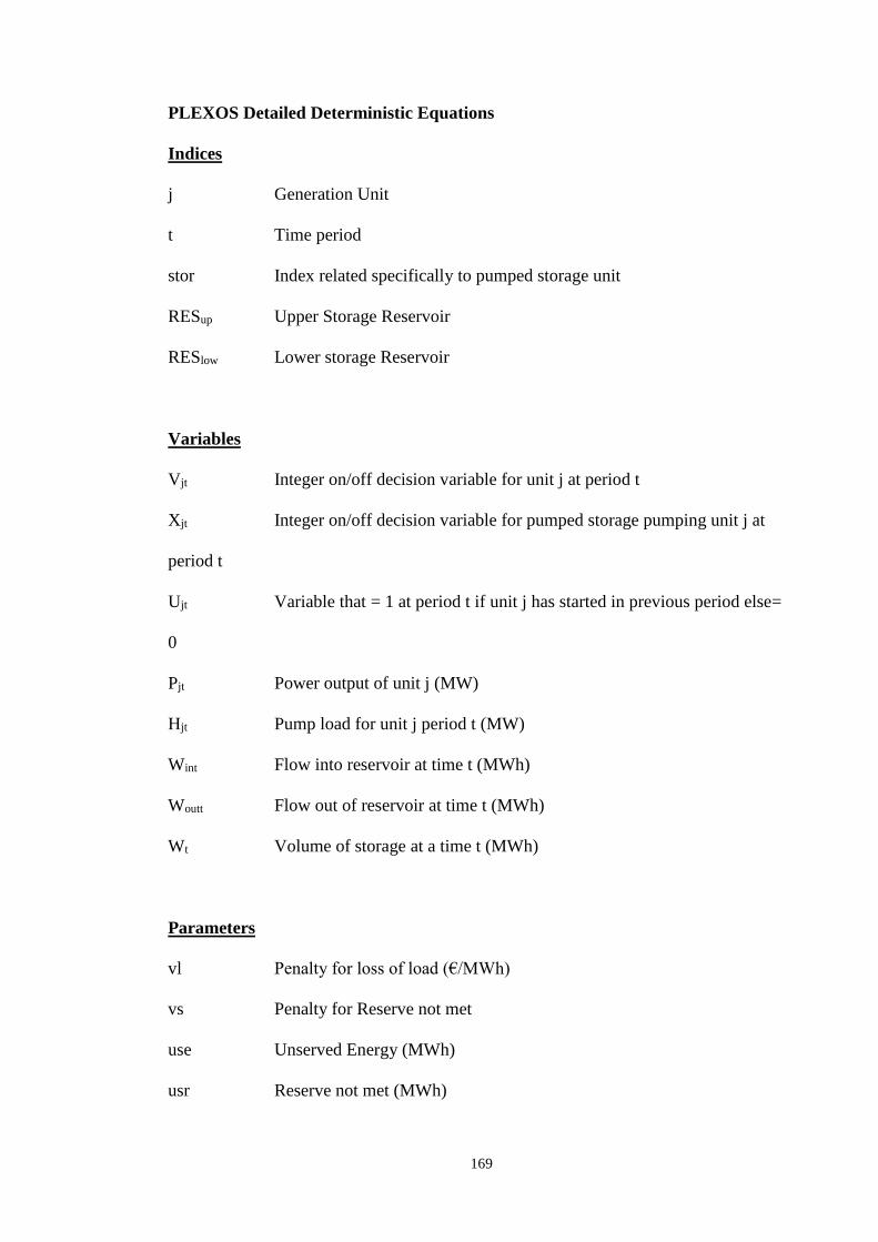
169

PLEXOS Detailed Deterministic Equations

Indices

j Generation Unit

t Time period

stor Index related specifically to pumped storage unit

RESup Upper Storage Reservoir

RESlow Lower storage Reservoir

Variables

Vjt Integer on/off decision variable for unit j at period t

Xjt Integer on/off decision variable for pumped storage pumping unit j at

period t

Ujt Variable that = 1 at period t if unit j has started in previous period else=

0

Pjt Power output of unit j (MW)

Hjt Pump load for unit j period t (MW)

Wint Flow into reservoir at time t (MWh)

Woutt Flow out of reservoir at time t (MWh)

Wt Volume of storage at a time t (MWh)

Parameters

vl Penalty for loss of load (€/MWh)

vs Penalty for Reserve not met

use Unserved Energy (MWh)

usr Reserve not met (MWh)

170

D Demand (MW)

OBJ Objective Function

njt No load cost unit j in period t (€)

cjt Start cost unit j in period t (€)

mjt Production Cost unit j in period t (€)

estor Efficiency of pumping unit (%)

Pmaxj Max power output of unit j (MW)

Pminj Min stable generation of unit j (MW)

Pmpmaxstor Max pumping capacity of pumping unit

Jj Available units in each generator

Jstor Number of pumping units

MRUj Maximum ramp up rate (MW/min)

MRDj Maximum ramp down rate (MW/min)

MUTj Minimum up time (hrs)

Ap Number of hours a unit must initially be online due to its MUT

constraint

WINT Initial volume of reservoir (GWh)

W Maximum volume of storage (GWh)

Objective Function

(7.1)

The objective function in PLEXOS is to minimise the start-up cost of each unit (start cost

(€) x number of starts of a unit) + the no load cost of each online unit + production

costs(fuel, carbon & VOM) of each online unit + the penalty for unserved load+ the

Tt

ttjtjtjtjtjtjt usrvsusevlPmVnUcMinOBJ .....

171

penalty of unserved reserve. The objective function is minimised within each simulation

period. The simulation must also satisfy the following constraints:

Energy Balance Equation

(7.2)

The energy balance equation states that the power output from each unit at each interval

minus the pump load from pumped storage units for each interval + unserved energy must

equal the demand for power at each interval. (Note that line losses can also be included

here but is not shown). As the penalty for unserved energy is high (approx. €10,000/MW)

and part of the objective function, the model will generally try to meet demand.

Operation Constraints on Units

Basic operational constraints that limit the operation and flexibility of units such as

maximum generation, minimum stable generation, minimum up/down times and ramp

rate. Equations (7.3) and (7.4) define the start definition of each unit and are used to track

the on/off status of units.

(7.3)

(7.4)

Max Export Capacity

A units power output cannot be greater than its maximum export capacity.

(7.5)

t

Tt

tjtjt DuseHP

1 jtjt UV 1t

011 jtjtjt UVV

0.max jtjjt VPP

172

Minimum Stable Generation

A units output must be greater than its minimum stable generation when the unit is online.

(7.6)

Pumping load must less than maximum pumping capacity for each pumping unit

(7.7)

The constraints below limit a pumped storage unit from pumping and generating at same

time.

(7.8)

(7.9)

Minimum Up Times

The variable Ap tracks if any starts have occurred on the unit inside the periods preceding

p with a window equal to MUT ( i.e. if no starts happen in the last MUT periods then Ap

will be zero, but if one (or more) starts have occurred then Ap will equal unity). The MUT

constraints then sets a lower bound on the unit commitment that is normally below zero,

but when a unit is started, the bound rises above zero until the minimum up time has

expired. This fractional lower bound when considered in an integer program forces the

unit to stay on for its minimum up time.

0.min jtjjt VPP

0.max jtstorjt XPmpH

1 jtjt XV storjwhere

jj VV JstorX j Jj

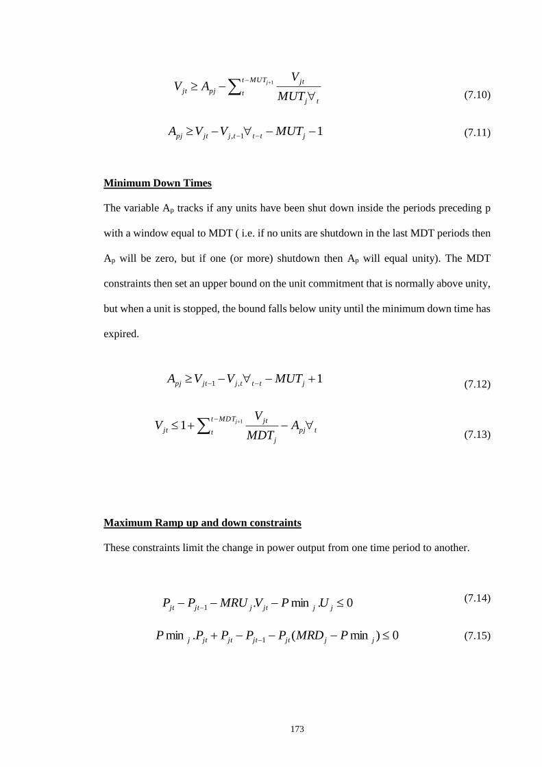
173

(7.10)

(7.11)

Minimum Down Times

The variable Ap tracks if any units have been shut down inside the periods preceding p

with a window equal to MDT ( i.e. if no units are shutdown in the last MDT periods then

Ap will be zero, but if one (or more) shutdown then Ap will equal unity). The MDT

constraints then set an upper bound on the unit commitment that is normally above unity,

but when a unit is stopped, the bound falls below unity until the minimum down time has

expired.

(7.12)

(7.13)

Maximum Ramp up and down constraints

These constraints limit the change in power output from one time period to another.

(7.14)

(7.15)

1,1 jtttjjtpj MUTVVA

1jMUTt

ttj

jt

pjjtMUT

VAV

11, jtttjjtpj MUTVVA

tpj

MDTt

tj

jt

jt AMDT

VV

j

1

1

0.min.1 jjjtjjtjt UPVMRUPP

0)min(.min 1 jjjtjtjtjtj PMRDPPPPP

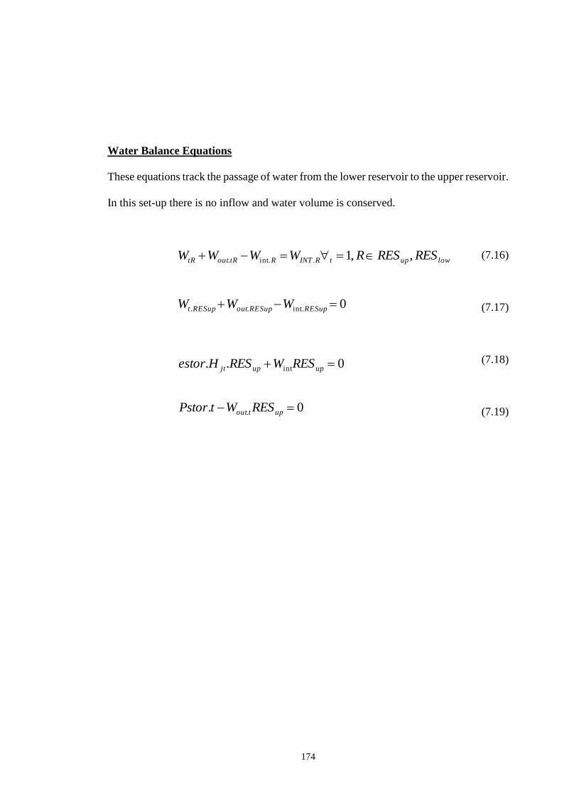
174

Water Balance Equations

These equations track the passage of water from the lower reservoir to the upper reservoir.

In this set-up there is no inflow and water volume is conserved.

(7.16)

(7.17)

(7.18)

(7.19)

lowuptRINTRtRouttR RESRESRWWWW ,,1..int.

0.int.. RESupRESupoutRESupt WWW

0.. int upupjt RESWRESHestor

0. . uptout RESWtPstor

175

PLEXOS Stochastic Equations

Indices

j Generation Unit

t Time period

s Stochastic scenario

stor Index related specifically to pumped storage unit

RESup Upper Storage Reservoir

RESlow Lower storage Reservoir

Variables

Vjt Integer on/off decision variable for unit j at period t

Xjt Integer on/off decision variable for pumped storage pumping unit j at

period t

Ujt Variable that = 1 at period t if unit j has started in previous period else=

0

Pjt Power output of unit j (MW)

Hjt Pump load for unit j period t (MW)

Wint Flow into reservoir at time t (MWh)

Woutt Flow out of reservoir at time t (MWh)

Wt Volume of storage at a time t (MWh)

Parameters

176

vl Penalty for loss of load (€/MWh)

vs Penalty for Reserve not met

use Unserved Energy (MWh)

usr Reserve not met (MWh)

D Demand (MW)

OBJ Objective Function

ks Probability of scenarios

njt No load cost unit j in period t (€)

cjt Start cost unit j in period t (€)

mjt Production Cost unit j in period t (€)

Jj Available units in each generator

Objective Function

(7.20

)

The objective function in PLEXOS using the scenario-wise decomposition method is to

minimise the start-up cost of each unit (start cost (€) x number of starts of a unit) + the

no load cost of each online unit + production costs(fuel, carbon & VOM) of each online

unit + the penalty for unserved load+ the penalty of unserved reserve. The objective

function is minimised within each simulation period and it must also satisfy the following

energy balance equation:

(7.21)

Ss Tt

tstsjtjtsjtjtsjtjts usrvskusevlkPmkVnkUckMinOBJ ..........

ts

Ss

tjst

Tt

jst DuseHP

177

List of Publications

Journal Publications

Cleary, B., Duffy, A., Bach, B.,Vitina, A.,O'Connor, A. and Conlon, M. (2015)

Estimating the electricity prices,generation costs and CO2 emissions of large scale wind

energy exports from Ireland to Great Britain, Energy Policy, vol. 91, pp. 38–48, 2015.

Cleary, B., Duffy, A., O Connor, A., Conlon, M., and Fthenakis, V. (2015) Assessing the

Economic Benefits of Compressed Air Energy Storage for Mitigating Wind

Curtailment, IEEE Transactions on Sustainable Energy, vol.6, no.3, pp.1021-1028.

Cleary, B., Duffy, A.,O'Connor, A., Conlon, M. (2015) Assessing the future economic

performance of wind generation in conjunction with compressed air energy storage in

the new proposed Irish electricity market. Economic and Business Letters, vol.4, no. 3

pp.87-97.

Conference Proceedings

Cleary, B., Duffy, A., O Connor, A., Conlon, M., and Fthenakis, V. (2013) Assessing

the benefits of compressed air energy storage on the 2020 Irish Power System, 48th

Universities' Power Engineering Conference (UPEC 2013), 2-5 September 2013, Dublin

Institute of Technology, Dublin, Ireland.

Cleary, B., Duffy, A., and O’Connor, A. (2012) Incorporation of Life Cycle Models in

determining Optimal Wind Energy Infrastructural Provision, Bridge and Concrete

Research in Ireland – BCRI 2012, 6 - 7 September 2012, Dublin, Ireland.

178

Cleary, B., Duffy, A., and O’Connor, A. (2012) Using life cycle assessment to compare

wind energy infrastructure, International Symposium on Life Cycle Assessment and

Construction, 10 - 12 July 2012, Nantes, France.

Reports

Duffy, A., Cleary, B., (2015). “Wind Energy Development in the Republic of Ireland,”

Chapter 3. Hand, M., ed., IEA Wind Task 26 - Wind Technology, Cost, and Performance

Trends: 2007–2012. NREL/TP-6A20-64332. Golden, CO: National Renewable Energy

Laboratory.