A Tale of Two Ports: The EconomicGeography of Inter-City Rivalry

Ngo Van LongMcGill University

Kar-yiu WongUniversity of Washington

August 7, 2001

Abstract

This paper examines how two geographically separated ports compete fora market consisting of manufacturing firms located between the two ports.There is a firm in each port, and these two firms, taking the infrastructureprovided by their governments as given, compete in a Bertrand sense. Thegovernments, however, can also compete in terms of investment in infrastruc-ture. This paper shows that there are cases in which both the firm and thegovernment in the port that has a longer history in the market may have thefirst mover advantage. In particular, the government can provide a crediblethreat by overinvesting in infrastructure.

This paper was presented at the conference “International Trade, IndustrialOrganization, and Asia” held at City University of Hong Kong, August 1999.Thanks are due to the participants of the conference for helpful comments.

c° 1999-2001 by Ngo Van Long and Kar-yiu Wong

1 Introduction

This paper presents a model of rivalry between two cities that are distributioncentres for goods produced in a long narrow region connecting the two cities.Rivalry between cities is a common feature of economic life. An example

that comes immediately to mind is the potential rivalry between Hong Kongand Shanghai. There are many other examples in the world that fit thepresent description. For example, in the United States, San Francisco andLos Angeles, and Seattle and Tacoma have long histories of competition.In Australia, Sydney and Melbourne have been known to be rivals for along time, both in the commercial and in the cultural spheres. In Canada,Montreal and Toronto used to be (almost) equal competitors. In Germany,Dresden and Leipzig have a long history of rivalry. Hong Kong and Singaporeare possible contenders for being the principal financial centre for East andSoutheast Asia (not including Japan.)When cities compete, the respective city governments may have an in-

centive to interfere, possibly to help locally based firms. This may reflect thedesire of each city to maximize a conventional social (or, rather, city-based)welfare function. Alternatively, one may adopt the political-economy viewthat city officials want to be reelected, and their campaign funds can be in-creased if they help local businesses (possibly at the expenses of local taxpayers.)Our paper is an attempt to model the commercial rivalry between two

cities. We abstract from considerations such as population size, agglomera-tion effects, labor market externalities, or diversification of business activi-ties1. Our main focus is on the investment in city infrastructure, such as theroad system, the law enforcement and regulatory system (e.g., how effectiveis the body that regulates the activities of the city stock exchange in HongKong, as compared with Singapore?). We model the rivalry between the twocities as follows. We assume that in each city there is a single distributor(or a cartel of distributors). The two distributors compete in service pricesthat they offer to manufacturing firms that are located in a long, narrow re-gion joining the two cities. Each distributor’s cost of supplying distributionservices depends on the quality of the city’s infrastructure, the provision ofwhich is the responsibility of the city’s government. The two governmentscompete against each other, because each wants its city to be the most pros-perous centre of commerce.In the model considered in the present paper, there are two levels of

1For models that deal with these issues, see, for example, North (1955), Thisse (1987),Glaeser et al. (1992), Fujita and Thisse (1996), Long and Soubeyran (1998), and Fujita,Krugman and Venebles (1999).

1

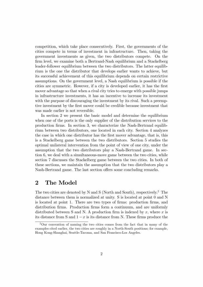
competition, which take place consecutively. First, the governments of thecities compete in terms of investment in infrastructure. Then, taking thegovernment investments as given, the two distributors compete. On thefirm level, we examine both a Bertrand-Nash equilibrium and a Stackelbergleader-follower equilibrium between the two distributors. The latter equilib-rium is the one the distributor that develops earlier wants to achieve, butits successful achievement of this equilibrium depends on certain restrictiveassumptions. On the government level, a Nash equilibrium is possible if thecities are symmetric. However, if a city is developed earlier, it has the firstmover advantage so that when a rival city tries to emerge with possible jumpsin infrastructure investments, it has an incentive to increase its investmentwith the purpose of discouraging the investment by its rival. Such a preemp-tive investment by the first mover could be credible because investment thatwas made earlier is not reversible.In section 2 we present the basic model and determine the equilibrium

when one of the ports is the only supplier of the distribution services to theproduction firms. In section 3, we characterize the Nash-Bertrand equilib-rium between two distributors, one located in each city. Section 4 analyzesthe case in which one distributor has the first mover advantage, that is, thisis a Stackelberg game between the two distributors. Section 5 studies theoptimal unilateral intervention from the point of view of one city, under theassumption that the two distributors play a Nash-Bertrand game. In sec-tion 6, we deal with a simultaneous-move game between the two cities, whilesection 7 discusses the Stackelberg game between the two cities. In both ofthese sections, we maintain the assumption that the two distributors play aNash-Bertrand game. The last section offers some concluding remarks.

2 The Model

The two cities are denoted by N and S (North and South), respectively.2 Thedistance between them is normalized at unity. S is located at point 0 and Nis located at point 1. There are two types of firms: production firms, anddistribution firms. Production firms form a continuum, and are uniformlydistributed between S and N. A production firm is indexed by x, where x isits distance from S and 1−x is its distance from N. These firms produce the

2Our convention of naming the two cities comes from the fact that in many of theexamples cited earlier, the two cities are roughly in a North-South positions; for example,Hong Kong-Shanghai, Seattle-Tacoma, and San Francisco-Los Angeles.

2

same good.3

For simplicity, assume that each production firm produces either one unitof output, or nothing. The cost of producing the output is a given constant,which is normalized as zero. The cost to firm x of shipping its output fromlocation x to S is bx2/2, and the cost of shipping the output from location xto N is (b/2)(1− x)2.4In city S, there is a single distribution firm labeled distributor S (or,

equivalently, a cartel of distributors) that provides the service of sending(and marketing) the goods to a foreign market. The cost of providing thisservice is CS per unit of good sold, which is taken as given by the distributor.The cost CS depends on the quality of the city’s infrastructure, IS, (such asthe quality of the road network, and of the law enforcement system), asdescribed by the following function,

CS = CS(IS),

where C 0S(IS) < 0 and C00S(IS) > 0.

5 It should be noted that IS is labeled asinvestment for simplicity, but it is in fact the accumulated investment in thepast less depreciation. It is therefore a stock, not a flow.Distributor charges a price θS ≥ CS, the same for all production firms,

for its distribution service.6 The world price of the good is P , assumed to begiven exogenously.In city N, there is a rival distributor labeled distributor N, with unit cost

of distribution CN given by

CN = CN(IN),

where C 0N(IN) < 0, C00N(IN) > 0.

3 Monopoly Distributor

We begin by focusing on one distributor. Suppose that initially the cost ofthe rival distributor in N is so high that it cannot compete with distributorS, e.g., the quality level IN is so low that CN(IN) > P. Then the southerndistributor is a monopolist.

3Many features of this model are borrowed from the spatial competition model ofHotelling (1927).

4Our assumption that the transport cost is quadratic in distance is in line withd’Aspremont et al. (1979).

5This means that an increase in the quality of the city’s infrastructure will lower thecost of the distribution service, but the rate of change in CS with respect to IS increaseswith the latter.

6Charging the same price to all production firms implies no price discrimination byeach distribution firm.

3

3.1 Optimal Production of Distributor S

The objective of distributor S is to maximize its profit by choosing a serviceprice θS and a cut off point xm ≤ 1 such that all firms with distance x > xmwill be excluded. For firms that are not excluded, the participation constraintis that they should earn non-negative profit. Formally, the distributor seeksto

maxθS ,xm

πS =Z xm

0(θS − CS)dx = (θS − CS)xm, (1)

subject to

P − θS − b2x2 ≥ 0, ∀x ∈ [0, xm], (2)

and0 ≤ xm ≤ 1. (3)

It is convenient to define the mark-up on distribution cost as z,

z = θS − CS. (4)

It is clear that problem (1) is equivalent to

maxz,xm

πS = zxm, (5)

subject to (3) and

P − CS − z − b2(xm)2 ≥ 0. (6)

To analyze problem (5), we make use of Figure 1. In the (x, z) space, wefirst construct various iso-profit contours, each of which corresponds to thesame profit. Each iso-profit contour, such as XZ, has a slope of

∂z

∂x

¯¯XZ

= −zx< 0, (7)

and is convex to the origin. Condition (6) is the area bounded from aboveby curve PC, which has a slope of

∂z

∂x

¯¯PC

= −bx < 0, (8)

and is concave to the origin. Constraint (3) refers to the region boundedby the vertical axis and the vertical line x = 1. The problem of the firmis to choose (x, z) that reaches the highest iso-profit contour subject to theconstraints (6) and (3). Depending on the nature of the solution, two casescan be distinguished.

4

The Whole Market Case (Corner Solution) – This case, in whichdistributor S serves all the production firms, is defined by the following con-dition:

P − CS ≥ 3b2. (9)

To see why there is a corner solution, note that at xm = 1, conditions (9)and (6) (the latter with an equality) imply that at (1, P − CS − b)

∂z

∂x

¯¯PC

≥ ∂z

∂x

¯¯XZ

, (10)

or that contour XZ is at least as steep as curve PC. This is the case shownin Figure 1 (with a strict inequality in condition (10)). The optimal pointwith the highest possible profit is E.At this point, condition (6) implies that the optimal price of the good is

θ∗S = P − b/2, giving a profit to the firm of

πSM = π∗SC(CS) = P − CS −b

2. (11)

The Partial Market Case (Interior Solution) – This case, in whichdistributor S serves some of the production firms closer to itself, is definedby the following condition:

P − CS < 3b

2. (12)

Let us suppose that starting from point E there is a drop in the price P,or a rise in the cost CS, or both, so that curve PC shifts down to, say, PC,satisfying condition (12). This produces a point of tangency, E, betweenPC and iso-profit contour XZ, it is optimal for distributor S to serve allthe production firms within the interval (0, x). Using (7) and (8), with (6)holding as an equality, we get the solution to the profit-maximizing problem:z∗ = 2(P − CS)/3, and

xm∗ =q2(P − CS)/(3b) (13)

θ∗S =2P + CS

3. (14)

Firm S is able to get a profit of

5

πSM = π∗SI(CS) =1√b

"2(P − CS)

3

#3/2, (15)

which is what contour XZ represents. Note that in these two cases with allproduction firms as price takers distributor S will set the service price θS sothat the production firm being served and farthest away from port S earns azero profit.

3.2 Optimal Investment by Government S

The government of port S is to choose the optimal investment in infras-tructure, IS, which determines the cost of distribution firm S takes as given.The government chooses IS to maximize the welfare function VS of the portdefined as

VS = πSM − (1 + β)IS, (16)

where β is the marginal cost of public finance7, and πSM is the profit of thedistribution firm as a monopolist, defined by either (11) or (15) dependingon whether an interior solution exists. Problem (16) yields the first ordercondition

π0SM(CS)C0S(IS) = (1 + β). (17)

In condition (17), π0SM(CS) = −1 and π00SM(CS) = 0 in the Whole Marketcase, or π0SM(CS) = −

q2(P − CS)/(3b) and π00SM(CS) = [2/(3b)]1/2[P −

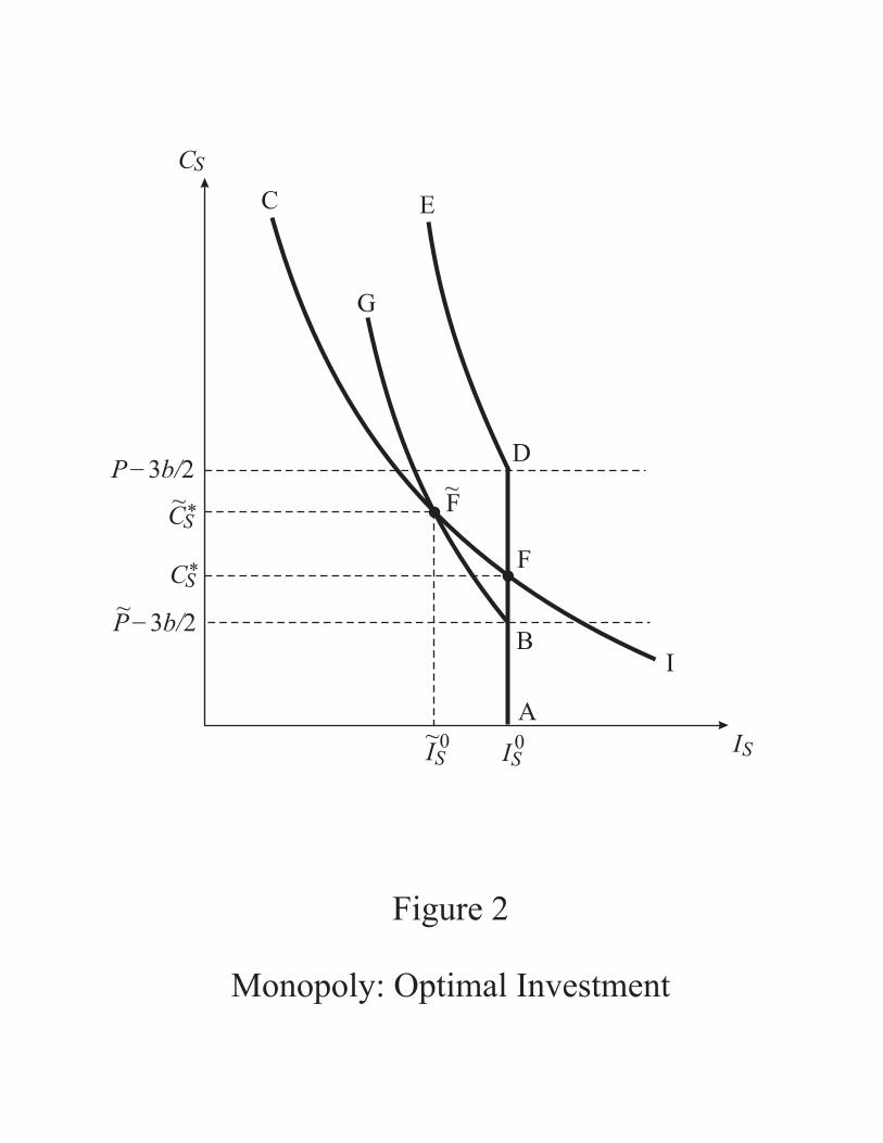
CS]−1/2 in the Partial Market case.When given the market price of the good, condition (17) is illustrated by

schedule ABFDE in Figure 2. This schedule has two components. SegmentABFD is a vertical line, corresponding to the Whole Market case (CS <P−3b/2), in which (17) reduces to an equation with one unknown, IS. Denotethe unique solution by I0S. Curve DE corresponds to the Partial Market case(CS > P − 3b/2). Condition (17) is differentiated to give the slope of curveDE:

dCSdIS

¯¯DE

= −π0SMC00S

C 0Sπ00SM

< 0. (18)

Also illustrated in Figure 2 is schedule CI, which represents CS = CS(IS),which, by assumption, is downward sloping and convex to the origin. Theintersection between schedules ABFDE and CI gives the optimal infrastruc-ture investment. At the initial market price, the optimal point occurs at F in

7It measures the deadweight loss caused by raising an extra dollar of tax.

6

the figure, with an infrastructure investment of I0S, leading to a service costof C∗S. Distributor S chooses to serve the whole market.

8

Suppose now that there is a significant decrease in P to, say, P . As aresult, the curve that represents condition (17) shifts to ABFG, with itsportion BFG corresponds to the case in which distributor S serves only partof the market. With the slope in (18) sufficiently large in magnitude, BFGcuts schedule CI at point F, leading to an optimal infrastructure investmentof I0S and a corresponding service cost of C

∗S.9 Making use of Figure 2 and

the previous analysis, the following proposition can easily be established, theproof of which is given in the appendix:

Proposition 1: (a) If currently CS ≤ P − 3b/2, a small rise in P will notaffect the government’s infrastructure investment while distributor S contin-ues to serve the whole market. The service price charged by distributor Sincreases by the same amount. (b) If currently CS > P −3b/2, a small rise inP will lead to an increase in the government’s infrastructure investment anda fall in the service cost, while distributor S serves more firms. The change inthe service price charged by distributor S is determined by condition (14).10

4 Duopoly in Distribution

Now consider the duopoly case, in which both distributors S and N mayprovide services to the production firms. These two distributors set serviceprices, θS and θN , respectively. To simplify the analysis, we assume that the

8As an example, one may take the special functional form

CS(IS) =γSIS,

where γS is a positive parameter. Assumingt that the market price is high enough so thatfirm S serves the whole market, we obtain the optimal investment condition

IS =

·γS1 + β

¸1/2.

9To satisfy the second-order condition, schedule GB is steeper than schedule CI, asshown in Figure 2. See the appendix for a proof.10Note that for simplicity we have not explicitly imposed the condition that investment

is irreversible, i.e., IS ≥ 0. Under irreversibility, there is an asymmetry between anincrease in P and a decrease in P. While a government may be interested in increasingits investment in response to an increase in P, it does not destroy some of its previousinvestment in the case of a drop in P.

7

market price is high enough so that if one distributor serves the market, itserves the whole market (the Whole Market case).11

Production firms take the service prices θN and θS as given, and choosethe distributor with the lower distribution cost. Denote xc as the firm indif-ferent between dealing with N or S, satisfying

θS +bx2c2= θN +

b(1− xc)22

,

orxc =

1

2+1

b(θN − θS) . (19)

Given that xc ∈ [0, 1], three cases can be distinguished:12

• Case S: θN − θS ≥ b/2. From (19), xc = 1, with all production firmsserved by distributor S.

• Case N: θS − θN ≥ b/2, implying that xc = 0, with all productionfirms served by distributor N .

• Case B: |θN − θS| < b/2. In this case, 0 < xc < 1, with distributorS serving firms located at (0, xc) while distributor N serving those at(xc, 1).

4.1 Reaction Functions of the Distributors

Define y ≡ θN − θS, and φ(y) ≡ xc. Let us first consider distributor S, whichmaximizes its profit, taking θN as given:

πS =Z φ(y)

0(θS − CS)dx = (θS − CS)φ(y), (20)

subject toP − θS − b[φ(y)]2/2 ≥ 0. (21)

Condition (21), which makes sure that all production firms served by thedistributor do not have negative profits, is assumed to be not binding. Thereaction curve of distributor S is derived as follows and is illustrated in Figure3:

Case N (region A): In this region, φ(y) = 0, and is bounded below bythe line XKL, θS = θN + (b/2), with distributor S serving no firm.

11This simplifies the analysis and guarantees interactions between the two distributors.12In all these cases, the market price is assumed to be high enough so that no production

firms concerned make a loss.

8

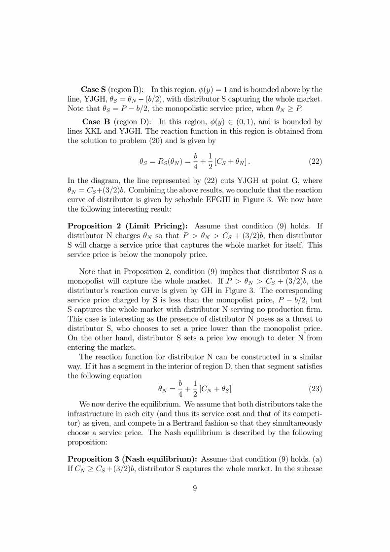
Case S (region B): In this region, φ(y) = 1 and is bounded above by theline, YJGH, θS = θN − (b/2), with distributor S capturing the whole market.Note that θS = P − b/2, the monopolistic service price, when θN ≥ P.

Case B (region D): In this region, φ(y) ∈ (0, 1), and is bounded bylines XKL and YJGH. The reaction function in this region is obtained fromthe solution to problem (20) and is given by

θS = RS(θN) =b

4+1

2[CS + θN ] . (22)

In the diagram, the line represented by (22) cuts YJGH at point G, whereθN = CS+(3/2)b. Combining the above results, we conclude that the reactioncurve of distributor is given by schedule EFGHI in Figure 3. We now havethe following interesting result:

Proposition 2 (Limit Pricing): Assume that condition (9) holds. Ifdistributor N charges θN so that P > θN > CS + (3/2)b, then distributorS will charge a service price that captures the whole market for itself. Thisservice price is below the monopoly price.

Note that in Proposition 2, condition (9) implies that distributor S as amonopolist will capture the whole market. If P > θN > CS + (3/2)b, thedistributor’s reaction curve is given by GH in Figure 3. The correspondingservice price charged by S is less than the monopolist price, P − b/2, butS captures the whole market with distributor N serving no production firm.This case is interesting as the presence of distributor N poses as a threat todistributor S, who chooses to set a price lower than the monopolist price.On the other hand, distributor S sets a price low enough to deter N fromentering the market.The reaction function for distributor N can be constructed in a similar

way. If it has a segment in the interior of region D, then that segment satisfiesthe following equation

θN =b

4+1

2[CN + θS] (23)

We now derive the equilibrium. We assume that both distributors take theinfrastructure in each city (and thus its service cost and that of its competi-tor) as given, and compete in a Bertrand fashion so that they simultaneouslychoose a service price. The Nash equilibrium is described by the followingproposition:

Proposition 3 (Nash equilibrium): Assume that condition (9) holds. (a)If CN ≥ CS+(3/2)b, distributor S captures the whole market. In the subcase

9

in which CN < P, distributor S charges a service price of

θS = CN − b2. (24)

If CN ≥ P, distributor S will charge the monopoly price θS = P − (b/2).(b) If CN < CS + (3/2)b, and CS < CN + (3/2)b, or more concisely,

|CN − CS| < (3/2)b, then we have an interior Nash equilibrium, satisfyingboth conditions (22) and (23), and the equilibrium charges are

θ∗S =b

2+1

3(2CS + CN) , (25)

and

θ∗N =b

2+1

3(2CN + CS) , (26)

provided that P is sufficiently great so that the indifferent production firmxc earns non-negative profit.13

(c) If CS ≥ CN +(3/2)b, distributor N captures the whole market . In thesubcase in which CS < P, distributor N charges a service price of

θN = CS − b2. (27)

If CS ≥ P, distributor N will charge the monopoly price θN = P − (b/2).

Remarks: The above proposition indicates that (i) distributor S will usethe limit pricing strategy if CN is below P but is sufficiently greater thanCS (precisely, CN ≥ CS + (3/2)b). If CN falls, then the limit price θS,given by (24) will also be adjusted downwards, and (ii) in the case whereboth distributors have positive market shares, a fall in CN will cause bothequilibrium charges to fall, but θS falls by less than θN .

4.2 Services Costs and Nash Equilibrium

Construct a diagram (Figure 4) in the (CN , CS) space, for a given P, whichwe assume to be greater than (3/2)b. We first examine how Case S isaffected by the distributors’ service costs. In region WS, which is defined byCN > P > CS+(3/2)b, firm S is the monopoly that serves the whole market,and its profit is

πSM = P − CS − (b/2) = πSM(CS), (28)

13This condition requires that P ≥ θ∗S + (b/2)x2c where xc = (1/2) + (1/3)b(CN − CS)and where θ∗S is as given above.

10

where the subscript M indicates that the distributor is in effect a full mo-nopolist. In triangle TN, which is defined by (3/2)b < CN < P , 0 < CS <P − (3/2)b, and CS < CN − 3b/2, both distributors offer a service price lessthan P , but distributor S captures the whole market by setting the limitprice θSL = CN − (b/2), thus earning the profit

πSL = θSL − CS = CN − CS − (b/2), (29)

where the subscript L indicates that the distributor is charging a limit price.We now turn to case N. In region WN defined by CS > P > CN + (3/2)b,firm N is the monopoly that serves the whole market, and its profit is

πNM = P − CS − (b/2) = πNM(CS). (30)

Similarly, in triangle TS defined by (3/2)b < CS < P , 0 < CN < P − (3/2)b,and CN < CS − 3b/2, both distributors offer a service price less than P , butdistributor N captures the whole market by setting the limit price θNL =CS − (b/2), thus earning the profit

πNL = θNL − CN = CS − CN − (b/2) > b. (31)

Finally, for case B, if the cost configuration (CN , CS) is in the region Xdefined by the square {(CN , CS) : 0 ≤ CN ≤ P , 0 ≤ CS ≤ P} excluding thetwo triangles TN and TS and a small region Q in the north-east corner ofthis square,14 then we have a unique and interior Nash equilibrium, i.e., bothdistributors have positive market shares. The market share of distributor Sat this equilibrium is

xS =1

2+1

3b[CN − CS] ,

and its Nash equilibrium profit is

πnashSI = [θS − CS]xS = 1

b

"b

2+1

3(CN − CS)

#2, (32)

where the subscript I indicates that the equilibrium is an interior one.

14In the small region Q, the costs of both distributors are so close to P that some subsetof production firms are not served by either distributor. The lower boundary of Q is givenby the condition that the marginal production firm earns zero profit and is indifferentbetween the two distributors.

11

5 Stackelberg Leadership by A Distributor

In the preceding sections, it was assumed that the two distributors play aNash-Bertrand game, choosing their service prices simultaneously. There are,however, some cases in which one of them can play as a Stackelberg leader.One possible case is now described.To describe such a possibility, let us first investigate more properties of

the distributors’ reaction curves. Consider Figure 5, which is obtained fromFigure 3, with some added details. Distributor S’s reaction function in Figure3 is reproduced in Figure 5, and is labelled JNKH, where K is the kink. Theco-ordinates of points J, K and H are respectively (0, CS/2+b/4), (CS+3b/2,CS+b) and (P , P−b/2). In the region in which both distributors serve someproduction firms (region D in Figure 3), the profit of distributor S is givenby

πS = [θS − CS]xc = [θS − CS]·1

2+1

b(θN − θS)

¸. (33)

The loci of (θN , θS) that give the same profit of distributor S, which can becalled an iso-profit contour, has the slope

∂θS∂θN

= −∂πS/∂θN∂πS/∂θS

=1

1− k , (34)

where

k =b+ 2 (θN − θS)

2 [θS − CS] .

Note that the slope of an iso-profit contour at a point on line JK, partof the distributor’s reaction curve, is infinity, implying that k = 1. Thisfurther implies that the slope of the contour is positive (negative) above(below) JK. In Figure 5, a Stackelberg equilibrium is depicted at point S,where distributor N’s reaction curve LNM is tangent to distributor S’s iso-profit curve πsS, which is higher that what distributor S can get at a Nashequilibrium. Since the slope of distributor N’s reaction curve NM is equal to2, k = 1/2 at point S.Now suppose that currently the infrastructure investments by government

N is very low, making the service cost of distributor N very high, so thatdistributor N chooses not to serve any production firms. So distributor Sis a monopolist and charges a service price of θmS = P − b/2. Suppose nowthat government invests significantly in infrastructures, lowering distributorN’s service cost so that its reaction curve is now represented by LNSM inFigure 5. If both distributors play Bertrand, the equilibrium is at point N.Distributor S will observe a considerable drop in its service price (to θnS) andprofit.

12

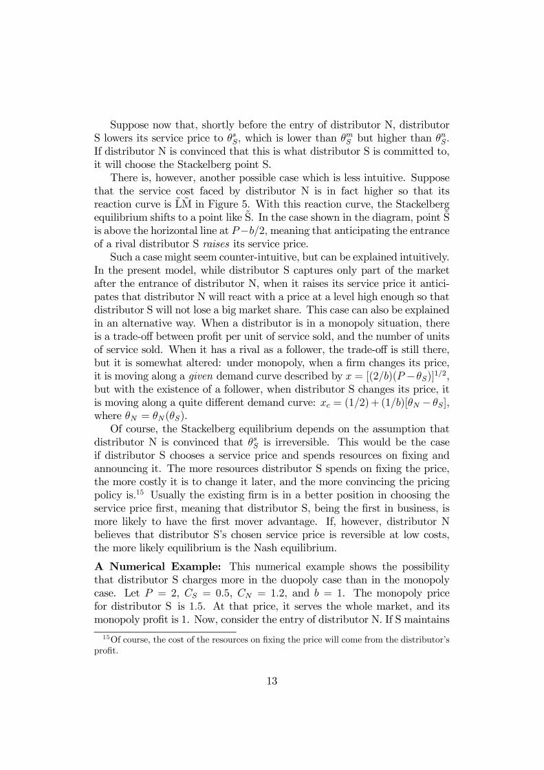
Suppose now that, shortly before the entry of distributor N, distributorS lowers its service price to θsS, which is lower than θmS but higher than θnS.If distributor N is convinced that this is what distributor S is committed to,it will choose the Stackelberg point S.There is, however, another possible case which is less intuitive. Suppose

that the service cost faced by distributor N is in fact higher so that itsreaction curve is LM in Figure 5. With this reaction curve, the Stackelbergequilibrium shifts to a point like S. In the case shown in the diagram, point Sis above the horizontal line at P−b/2,meaning that anticipating the entranceof a rival distributor S raises its service price.Such a case might seem counter-intuitive, but can be explained intuitively.

In the present model, while distributor S captures only part of the marketafter the entrance of distributor N, when it raises its service price it antici-pates that distributor N will react with a price at a level high enough so thatdistributor S will not lose a big market share. This case can also be explainedin an alternative way. When a distributor is in a monopoly situation, thereis a trade-off between profit per unit of service sold, and the number of unitsof service sold. When it has a rival as a follower, the trade-off is still there,but it is somewhat altered: under monopoly, when a firm changes its price,it is moving along a given demand curve described by x = [(2/b)(P −θS)]

1/2,but with the existence of a follower, when distributor S changes its price, itis moving along a quite different demand curve: xc = (1/2)+ (1/b)[θN − θS],where θN = θN(θS).Of course, the Stackelberg equilibrium depends on the assumption that

distributor N is convinced that θsS is irreversible. This would be the caseif distributor S chooses a service price and spends resources on fixing andannouncing it. The more resources distributor S spends on fixing the price,the more costly it is to change it later, and the more convincing the pricingpolicy is.15 Usually the existing firm is in a better position in choosing theservice price first, meaning that distributor S, being the first in business, ismore likely to have the first mover advantage. If, however, distributor Nbelieves that distributor S’s chosen service price is reversible at low costs,the more likely equilibrium is the Nash equilibrium.

A Numerical Example: This numerical example shows the possibilitythat distributor S charges more in the duopoly case than in the monopolycase. Let P = 2, CS = 0.5, CN = 1.2, and b = 1. The monopoly pricefor distributor S is 1.5. At that price, it serves the whole market, and itsmonopoly profit is 1. Now, consider the entry of distributor N. If S maintains

15Of course, the cost of the resources on fixing the price will come from the distributor’sprofit.

13

the previous monopoly service price θS = 1.5, then N will charge θN = 1.6,and S’s market share will fall to 0.6, and its profit will be πS = 0.6. Clearly,S can do better by maximizing (33) where θN = θN(θS) as given by (23).This yields θS = 1.60, and θN = 1.65, resulting in a smaller market share forS, xc = 0.55 and a higher profit, πS = 0.605.

6 Optimal Unilateral Intervention

Assume that initially the costs are C0S and C0N , and the equilibrium is an

interior one, i.e., both distributors serve some production firms. Supposethat the government of city S wants to maximize the welfare function VS bychoosing investment level IS, taking as given the amount IN . We assumethat government S first chooses a new (possibly higher) investment level,with government N remaining passive. Both distributors take the investmentlevels as given and compete in a Bertrand fashion.Let us assume that by spending IS > 0, the cost CS will fall to a level

below C0S. This fall is represented by a function FS(IS), where FS(0) = 0,F 0S(.) < 0, and F

00S (.) > 0, and CS = C

0S − FS(IS).16 The government of city

S maximizes

VS =1

b

"b

2+1

3(CN − CS)

#2− (1 + β)IS. (35)

The first-order condition isdVSdIS

= −ω(IN , I∗S)F 0S(I∗S)− (1 + β) ≤ 0, = 0 if I∗S > 0, (36)

whereω(IN , I

∗S) =

1

3+1

9b

³C0N − FS(IN)− C0S + FS(I∗S)

´> 0, (37)

and at an interior Nash equilibrium |CN − CS| < (3/2)b. It follows thatcondition (36) is satisfied at some I∗S > 0 if |F 0(0)| > (1 + β)/ω(I 0N , 0), thatis, if the first dollar spent on investment has a very substantial marginaleffect on cost reduction. In what follows we assume that this is the case, sothat, given IN , at the optimal investment level I∗S, we have

F 0(I∗S) = −(1 + β)/ω(IN , I∗S). (38)

The second-order condition isd2VSdI2S

= −ω(IN , I∗S)F 00(I∗S)−1

9b[F 0(I∗S)]

2 ≡ ∆S < 0, (39)

16Notice that it is assumed that the fall in cost is independent of the existing level ofcost. A more general formulation would have C0S appear as a parameter in the functionFS .

14

which is satisfied.

Proposition 4: Assume that |F 0S(0)| > (1 + β)/ω(IN , 0). Then the opti-mal policy for the government of S is to raise taxes to invest in the city’sinfrastructure, until condition (38) is satisfied.

Remark: Because of upward sloping reaction functions, if we are consideringoptimal output tax, we would get a result similar to that of Eaton andGrossman (1986), who found that if a foreign firm and a home firm competein prices (and their reaction functions have positive slope) then the optimalpolicy for the home government is to increase the cost of the home firm bytaxing its exports. In our model, we deal with modifying real costs, and theoptimal policy is to reduce the cost of the home firm, if the initial cost is high.There are two features worth noting. Firstly, since the production firms thatare located on the long narrow region linking N and S are the purchasers ofthe services, they are the analog of the consumers in the third market in theEaton-Grossman model. However, in our model, the “demand” for serviceof S, given by (19), remains unchanged if both distributors slightly raisetheir service prices by the same amount. This is not the case in the Eaton-Grossman model. The second feature is that while in the Eaton-Grossmanmodel a dollar of subsidy reduces the cost of the home firm by a dollar,in our model a dollar of spending in infrastructure reduces the cost of thedistributor by F 0S which is not a constant (recall that F

00S > 0).

7 Simultaneous Government Policies

Now suppose that both cities are engaged in the infrastructure-investmentgame. The governments first choose an investment level simultaneously.Then the distributors, taking these investment levels as given, compete ina Bertrand fashion.For a given initial pair (C0S, C

0N), let us find the reaction function of each

city. From (36), we obtain city S’s reaction function IS = rS(IN), with anegative slope given by

dISdIN

¯¯S

≡ r0S(IN) =1

∆S

"F 0NF

0S

9b

#< 0, (40)

where ∆S is defined in (39). By condition (40), the magnitude of the slopeis less than unity if |F 0S(IS)| ≥ |F 0N(IN)|. The reaction function IS = rS(IN)is illustrated in Figure 6. Note that there is a maximum value of city S’sinvestment, as represented by the flat part AB of the reaction schedule.

15

This is the optimal investment of the government when distributor S is amonopolist.17

Similarly, for city N, the reaction function of government N is IN =rN(IS), which satisfies

dINdIS

¯¯N

≡ r0N(IS) =1

∆N

"F 0NF

0S

9b

#< 0, (41)

where ∆N is defined in a similar way to ∆S above. The reaction function isillustrated in Figure 6, with CD representing the maximum value of govern-ment N’s investment.In general, there is the possibility of multiple equilibria, as illustrated in

Figure 6. If the initial costs C0S and C0N are identical, and the functions FN(.)

and FS(.) are the same, then there exists a symmetric Nash equilibrium thatis stable, see point E3 in Figure 6. However, there may exist non-symmetricstable equilibria, such as points E1 and E5.In the case of multiple equilibria, it can be shown, by construction of

iso-welfare curves, Vi = constant (i = S,N), that city N prefers E5 to E3 toE1, and similarly, city S prefers E1 to E3 to E5.In what follows, we will restrict attention to the case where there is only

one Nash equilibrium. We assume that such equilibrium is stable. See Figure7, where the unique Nash equilibrium is E.

8 Stackelberg Game between Cities

As explained earlier, it is possible that one of the cities, say S, develops first.Suppose that initially city N has a very low investment in infrastructure,such as I0N so that distributor N cannot compete with distributor S.

18 In theabsence of active investment by city N, the government of S and distributorS reach the monopoly equilibrium as described in Section 3. This equilibriumcan be represented by a point in between A and B in Figure 7. Note thatthe investment by city N that corresponds to point B, denoted by IBN inFigure 7, is the one that will yield a service cost to distributor N equal to themarket price of the good, CN = P. With this service cost and market price,distributor N will not want to provide any distribution service.Suppose now that city N invests in infrastructure. What is the new equi-

librium? The reaction curve of city S is ABEF. Since city S develops earlier,it has the first mover advantage. Note that AB is a horizontal line, showing

17Point B gives the value of IN that gives a service cost CN = P.18In other words, we assume that CN (I0N ) > P.

16

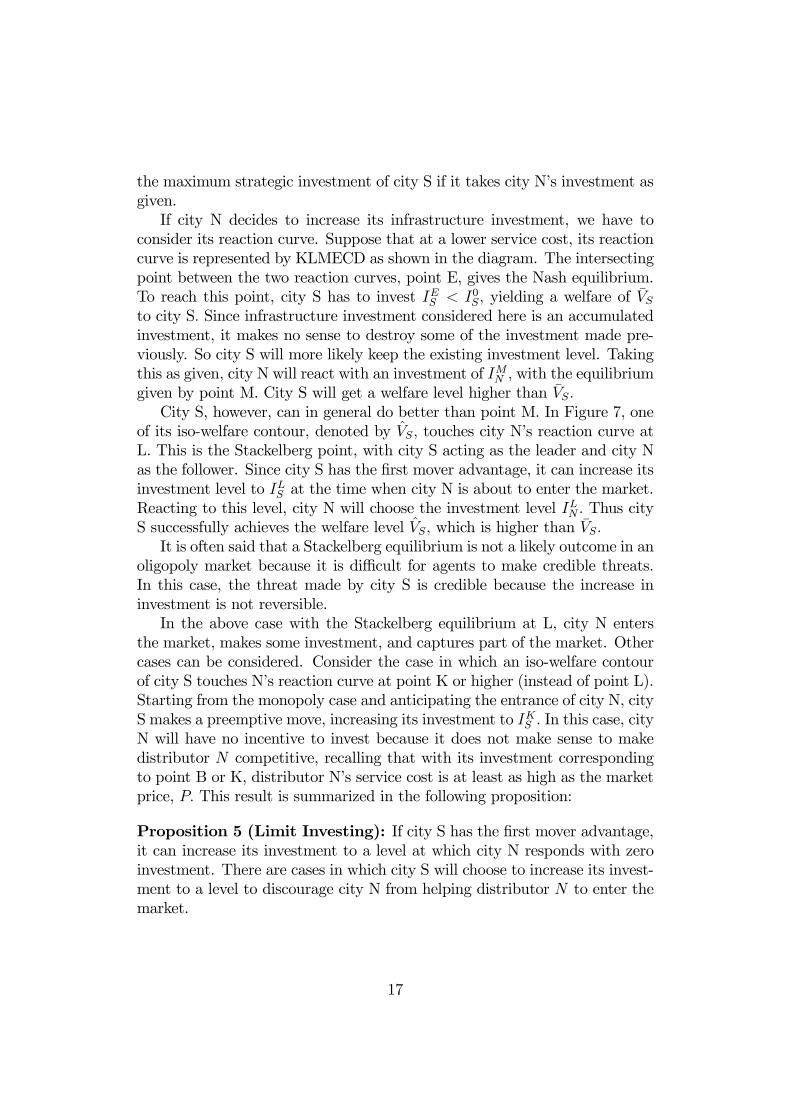
the maximum strategic investment of city S if it takes city N’s investment asgiven.If city N decides to increase its infrastructure investment, we have to

consider its reaction curve. Suppose that at a lower service cost, its reactioncurve is represented by KLMECD as shown in the diagram. The intersectingpoint between the two reaction curves, point E, gives the Nash equilibrium.To reach this point, city S has to invest IES < I0S, yielding a welfare of VSto city S. Since infrastructure investment considered here is an accumulatedinvestment, it makes no sense to destroy some of the investment made pre-viously. So city S will more likely keep the existing investment level. Takingthis as given, city N will react with an investment of IMN , with the equilibriumgiven by point M. City S will get a welfare level higher than VS.City S, however, can in general do better than point M. In Figure 7, one

of its iso-welfare contour, denoted by VS, touches city N’s reaction curve atL. This is the Stackelberg point, with city S acting as the leader and city Nas the follower. Since city S has the first mover advantage, it can increase itsinvestment level to ILS at the time when city N is about to enter the market.Reacting to this level, city N will choose the investment level ILN . Thus cityS successfully achieves the welfare level VS, which is higher than VS.It is often said that a Stackelberg equilibrium is not a likely outcome in an

oligopoly market because it is difficult for agents to make credible threats.In this case, the threat made by city S is credible because the increase ininvestment is not reversible.In the above case with the Stackelberg equilibrium at L, city N enters

the market, makes some investment, and captures part of the market. Othercases can be considered. Consider the case in which an iso-welfare contourof city S touches N’s reaction curve at point K or higher (instead of point L).Starting from the monopoly case and anticipating the entrance of city N, cityS makes a preemptive move, increasing its investment to IKS . In this case, cityN will have no incentive to invest because it does not make sense to makedistributor N competitive, recalling that with its investment correspondingto point B or K, distributor N’s service cost is at least as high as the marketprice, P. This result is summarized in the following proposition:

Proposition 5 (Limit Investing): If city S has the first mover advantage,it can increase its investment to a level at which city N responds with zeroinvestment. There are cases in which city S will choose to increase its invest-ment to a level to discourage city N from helping distributor N to enter themarket.

17

9 Concluding Remarks

We have modelled the rivalry between two cities, focussing on infrastructureinvestment. We have shown that at the firm level, equilibrium may involvelimit pricing by a distributor. At the city level, preemptive investment by thecity that exists first is possible. Such preemptive investment could discouragethe latecomer from entering the market.There are a few issues that could be taken up in future research. Firstly,

what is the optimal cooperative outcome, where the cooperation may bebetween the two cities, at the expense of the production firms in the longnarrow strip that join them? One can also involve the welfare of the owners ofthese firms as well. Secondly, cities may compete in more than one dimension.When the model is extended to allow for this, is it possible that the non-cooperative equilibrium may maximize, rather than minimize, the differencebetween the two cities? Could it be the case that one city becomes a financialcentre while the other becomes a goods distribution centre?

18

Appendix

Proof of Proposition 1: The proof of part (a) is simple and is omitted.To prove (b), write the first-order condition (17) as

G(P, IS) ≡ π0SM(CS(IS))C0S(IS)− (1 + β) = 0. (42)

The second-order condition is

∂G

∂IS= (C 0S)

2π00SM + π0SMC

00S,

is assumed to be negative, i.e.,

−π0SMC00S

C 0Sπ00SM

< C 0S,

or in Figure 2, curve CI is less steep than the GB curve. The response of ISto an increase in P is obtained from (42):

dISdP

= − ∂G/∂P

∂G/∂IS=

π00SMC0S

(C 0S)2 π00SM + π0SMC

00S

> 0. (43)

From (13), (14) and (43),

dxm∗

dP=

s3b

8(P − CS)Ã1− C 0S

dISdP

!> 0

dθ∗SdP

=2

3+1

3C 0SdISdP.

The sign of dθ∗S/dP is ambiguous.

19

O

Figure 1

Monopoly: Optimal Market Size

P Cs_

P Cs_ _

b/2

1 x

X

Z

E

z

Z~

E~..

P Cs_~ ~

P

P

CC~

~

X~

CS

IS

C

I

..P

_3 2b/

F

F~

A

B

D

E

G

CS*

CS*

~

P_

3 2b/~

Figure 2

Monopoly: Optimal Investment

IS0IS

0~

Figure 3

Reaction Functions and Nash Equilibrium

�S

�Nb_2

b

b/ C4 + S/2

/2

b_4

CS+CN__2

+

P_ b_

2

CS +b

3b__2

P_

P

Pb_2

RS(�N

)

RN

(S)

D

B:

( ) = 0y�

_ b_2

CN

E

FG

H I

J

KL

M

( ) = 1y�

A:

�

Y

X

Figure 4

Nash Equilibrium and Cost Structures

3b2 P

_

P

P

CS

CN

3b2

3b2

P_ 3b

2

WN

WS

TN

�SL* = CN

_ b2

TS Q

�S* =

P_ b

2

X

Figure 5

Distributor S as a Stackelberg Leader

�S

�Nb_2

b

b/ C4 + S/2

/2

P_

P

Pb_2

. .M

LJ

NK

H

S

S~

M

L

~

.

~

.

�Ss

�Ss~

�Ss

�Ss

�Sm

~

�Sn

IS

IN

rN ( )IS

r N( )IS

..

..

.

E1

E3

E2

E4E5

Figure 6

Nash Equilibria for Government Policies

45o

AB

C

D

IS

IN

Figure 7

Port S as a Stackelberg Leader

.E

.L

rN ( )IS

r N( )IS

VS

_

VS

A B

C

D

.M

EINL

IS0

ISE

ISK

NIINMIN

B

K.IS

L

F

References

[1] d’Aspremont, Claude J., Jean Gabszewicz, and Jacques-François Thisse(1979), “On Hotelling’s Stability in Competition,” Econometrica, 17:1145—51.

[2] Eaton, Jonathan, and Gene M. Grossman (1986), “Optimal Trade andIndustrial Policy under Oligopoly,” Quarterly Journal of Economics, 101:385—406.

[3] Fujita, Masahisa and Jacques-François Thisse (1996), “Economics of Ag-glomeration,” Journal of International and Japanese Economies, 10 (4,December): 339—78.

[4] Fujita, Masahisa, Paul Krugman, and Anthony J. Venebles (1999), TheSpatial Economy: Cities, Regions, and International Trade, Cambridge,MA: MIT Press.

[5] Glaeser, E., H.D. Kallal, J. A. Scheinkman, and A. Shleifer (1992),“Growth in Cities,” Journal of Political Economy, 100: 1126—56.

[6] Hotelling, Harold (1929), “Stability in Competition,” Economic Journal,39: 41-57.

[7] Long, Ngo Van and Antoine Soubeyran (1998), “R&D Spillovers andLocation Choice under Cournot Rivalry,” Pacific Economic Review, 3(2): 105—119.

[8] North, Douglas (1955), “Location Theory and Regional EconomicGrowth,” Journal of Political Economy, 62: 243—258.

[9] Thisse, Jacques-François (1987), “Location Theory, Regional Science, andEconomics,” Journal of Regional Science, 27: 519—528.

20