1

A Systematic Study ofFunctional Language Implementations

Rémi Douence and Pascal Fradet

INRIA / IRISA

Campus de Beaulieu, 35042 Rennes Cedex, France

douence@irisa.fr fradet@irisa.fr

Abstract: We introduce a unified framework to describe, relate, compare and classify functional lan-guage implementations. The compilation process is expressed as a succession of program transforma-tions in the common framework. At each step, different transformations model fundamental choices. Abenefit of this approach is to structure and decompose the implementation process. The correctnessproofs can be tackled independently for each step and amount to proving program transformations inthe functional world. This approach also paves the way to formal comparisons by making it possible toestimate the complexity of individual transformations or compositions of them. Our study aims at cov-ering the whole known design space of sequential functional languages implementations. In particular,we consider call-by-value, call-by-name and call-by-need reduction strategies as well as environmentand graph-based implementations. We describe for each compilation step the diverse alternatives asprogram transformations. In some cases, we illustrate how to compare or relate compilation tech-niques, express global optimizations or hybrid implementations. We also provide a classification ofwell-known abstract machines.

Key-words: functional programming, compilers, optimization, program transformation, combinators

1 INTRODUCTION

One of the most studied issues concerning functional languages is their implementation.Since Landin’s seminal proposal, 30 years ago [31], a plethora of new abstract machines orcompilation techniques have been proposed. The list of existing abstract machines includesthe SECD [31], the Cam [10], the CMCM [36], the Tim [20], the Zam [32], the G-machine[27] and the Krivine-machine [11]. Other implementations are not described via an abstractmachine but as a collection of transformations or compilation techniques such as compilersbased on continuation passing style (CPS) [2][22][30][52]. Furthermore, numerous paperspresent optimizations often adapted to a specific abstract machine or a specific approach[3][8][28]. Looking at this myriad of distinct works, obvious questions spring to mind: whatare the fundamental choices? What are the respective benefits of these alternatives? What areprecisely the common points and differences between two compilers? Can a particular opti-mization, designed for machineA, be adapted to machineB? One finds comparatively veryfew papers devoted to these questions. There have been studies of the relationship betweentwo individual machines [37][43] but, to the best of our knowledge, no global approach tostudy implementations.

2

The goal of this paper is to fill this gap by introducing a unified framework to describe,relate, compare and classify functional language implementations. Our approach is to ex-press the whole compilation process as a succession of program transformations. The com-mon framework considered here is a hierarchy of intermediate languages all of which aresubsets of the lambda-calculus. Our description of an implementation consists of a series oftransformationsΛ T1→ Λ1 →T2 … →Tn Λn, each one compiling a particular task by mappingan expression from one intermediate language into another. The last languageΛn consists offunctional expressions that can be seen as assembly code (essentially, combinators with ex-plicit sequencing and calls). For each step, different transformations are designed to repre-sent fundamental choices or optimizations. A benefit of this approach is to structure anddecompose the implementation process. Two seemingly disparate implementations can befound to share some compilation steps. This approach also has interesting payoffs as far ascorrectness proofs and comparisons are concerned. The correctness of each step can be tack-led independently and amounts to proving a program transformation in the functional world.Our approach also paves the way to formal comparisons by estimating the complexity of in-dividual transformations or compositions of them.

We concentrate on pureλ-expressions and our source languageΛ is E ::= x | λx.E | E1 E2.Most fundamental choices can be described using this simple language. The two steps whichcause the greatest impact on the compiler are the implementation of the reduction strategy(searching for the next redex) and the environment management (compilation of theβ-re-duction). Other steps include the implementation of control transfers (calls & returns), theimplementation of closure sharing and update (implied by the call-by-need strategy), therepresentation of components like the data stack or environments and various optimizations.

In Section 2 we describe the framework used to model the compilation process. In Sec-tion 3, we present the alternatives to compile the reduction strategy (i.e. call-by-value andcall-by-name). The compilation of control used by graph reducers is peculiar. A separatesection (3.3) is dedicated to this point. Section 3 ends with a comparison of two compilationtechniques of call-by-value and a study of the relationship between the compilation of con-trol in the environment and graph-based models. Section 4 (resp. Section 5) describes thedifferent options to compile theβ-reduction (resp. the control transfers). Call-by-need isnothing but call-by-name with redex sharing and update and we present in Section 6 how itcan be expressed in our framework. Section 7 embodies our study in a taxonomy of classicalfunctional implementations. In Section 8, we outline some extensions and applications of theframework. Section 9 is devoted to a review of related work and Section 10 concludes by in-dicating directions for future research.

In order to alleviate the presentation, some more involved material such as proofs, vari-ants of transformations and other technical details have been kept out of the main text. Werefer the motivated reader to the (electronically published) appendix. References to the ap-pendix are noted “

x”. A previous conference paper [16] concentrates on call-by-value and

can be used as a short introduction to this work. Additional details can also be found in twocompanion technical reports ([17], [18]) and a PhD thesis [19].

3

2 GENERAL FRAMEWORK

Each compilation step is represented by a transformation from an intermediate language toanother one that is closer to machine code. In this paper, the whole implementation processis described via a transformation sequenceΛ T1→ Λs

T2→ ΛeT3→ Λk

T4→ Λh starting withΛand involving four intermediate languages (very close to each other). This framework pos-sesses several benefits:

• It has astrong formal basis. Each intermediate language can be seen either as a formalsystem with its own conversion rules or as a subset of theλ-calculus by defining its con-structs asλ-expressions. The intermediate languages share many laws and properties; themost important being that every reduction strategy is normalizing. These features facili-tate program transformations, correctness proofs and comparisons.

• It is (relatively)abstract. Since we want to model completely and precisely implementa-tions, the intermediate languages must come closer to an assembly language as weprogress in the description. The framework nevertheless possesses many abstract featureswhich do not lessen its precision. The combinators of the intermediate languages andtheir conversion rules allow a more abstract description of notions such as instructions,sequencing, stacks,… than an encoding asλ-expressions. As a consequence, the compi-lation of control is expressed more abstractly than using CPS expressions and the imple-mentation of components (e.g. data stack, environment stack,…) is a separate step.

• It is modular. Each transformation implements one compilation step and can be definedindependently from the former steps. Transformations implementing different steps arefreely composed to specify implementations. Transformations implementing the samestep represent different choices and can be compared.

• It is extendable. New intermediate languages and transformations can be defined and in-serted into the transformation sequence to model new compilation steps (e.g. register al-location).

2.1 Overview

The first step is the compilation of control which is described by transformations fromΛ toΛs. The intermediate languageΛs (Figure 1) is defined using the combinatorso, pushs and anew form ofλ-abstractionλsx.E. Intuitively, o is a sequencing operator andE1 o E2 can beread “evaluateE1 then evaluateE2”, pushs E returnsE as a result andλsx.E binds the previ-ous intermediate result tox before evaluatingE. The pair (pushs, λs) specifies a component(noteds) storing intermediate results (e.g. a data stack). So,pushs andλs can be seen as“store” and “fetch” in s.

The most notable syntactic feature ofΛs is that it rules out unrestricted applications. Itsmain property is that the choice of the next weak redex is not relevant anymore: all weak re-dexes are needed. This is the key point to view transformations fromΛ to Λs as compilingthe evaluation strategy.

Transformations fromΛs to Λe are used to compile theβ-reduction. The languageΛeexcludes unrestricted uses of variables which are now only needed to define macro-combina-

4

tors. The encoding of environment management is made possible using the new pair(pushe, λe). They behave exactly aspushs andλs; they just act on a (at least conceptually)

different componente (e.g. a stack of environments).

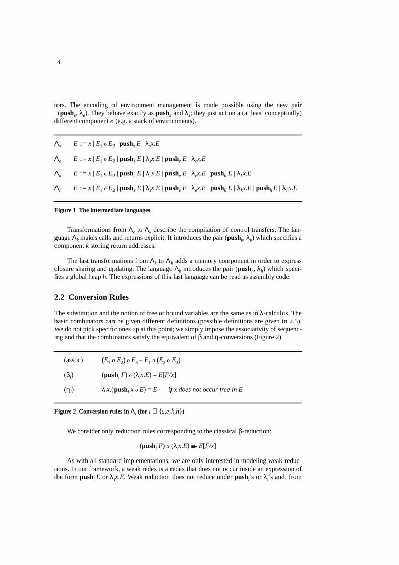
Λs E ::= x | E1 o E2 | pushs E | λsx.E

Λe E ::= x | E1 o E2 | pushs E | λsx.E | pushe E | λex.E

Λk E ::= x | E1 o E2 | pushs E | λsx.E | pushe E | λex.E | pushk E | λkx.E

Λh E ::= x | E1 o E2 | pushs E | λsx.E | pushe E | λex.E | pushk E | λkx.E | pushh E | λhx.E

Figure 1 The intermediate languages

Transformations fromΛe to Λk describe the compilation of control transfers. The lan-guageΛk makes calls and returns explicit. It introduces the pair (pushk, λk) which specifies acomponentk storing return addresses.

The last transformations fromΛk to Λh adds a memory component in order to expressclosure sharing and updating. The languageΛh introduces the pair (pushh, λh) which speci-fies a global heaph. The expressions of this last language can be read as assembly code.

2.2 Conversion Rules

The substitution and the notion of free or bound variables are the same as inλ-calculus. Thebasic combinators can be given different definitions (possible definitions are given in 2.5).We do not pick specific ones up at this point; we simply impose the associativity of sequenc-ing and that the combinators satisfy the equivalent ofβ andη-conversions (Figure 2).

(assoc) (E1 o E2) o E3 = E1 o (E2 o E3)

(βi) (pushi F) o (λix.E) = E[F/x]

(ηi) λix.(pushi x o E) = E if x does not occur free in E

Figure 2 Conversion rules inΛi (for i ∈ s,e,k,h )

We consider only reduction rules corresponding to the classicalβ-reduction:

(pushi F) o (λix.E) E[F/x]

As with all standard implementations, we are only interested in modeling weak reduc-tions. In our framework, a weak redex is a redex that does not occur inside an expression ofthe formpushi E or λix.E. Weak reduction does not reduce underpushi’s or λi’s and, from

5

here on, we write “redex” (resp. reduction, normal form) for weak redex (resp. weak reduc-tion, weak normal form).

The following example illustratesβi-reduction (note thatpushs F o λsz.G is not a (weak)redex of the global expression).

pushe E o pushs (pushs F o λsz.G) o λsx.λey.pushs(pushe y o x)

pushe E o λey.pushs(pushe y o pushs F o λsz.G)

pushs (pusheE o pushs F o λsz.G)

Any two redexes are clearly disjoint and theβi-reductions are left-linear so the term re-writing system is orthogonal hence confluent [29]. Alternatively, it is very easy to show thatthe relation is strongly confluent therefore confluenta . Furthermore, any redex is needed(a rewrite cannot suppress a redex) thus

Property 1 All Λi reduction strategies are normalizing.

This property is the key point to view transformations fromΛ to Λs as compiling the re-duction order.

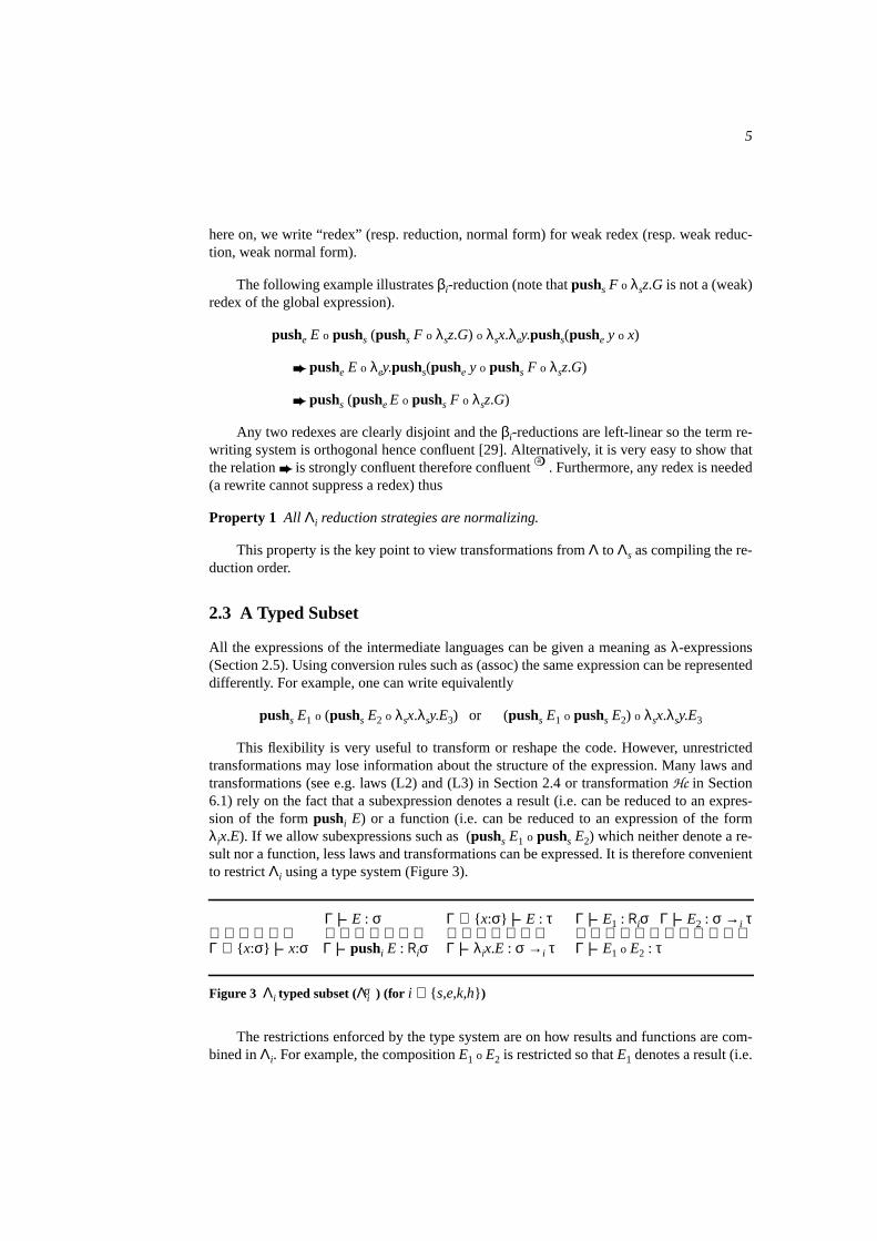
2.3 A Typed Subset

All the expressions of the intermediate languages can be given a meaning asλ-expressions(Section 2.5). Using conversion rules such as (assoc) the same expression can be representeddifferently. For example, one can write equivalently

pushs E1 o (pushs E2 o λsx.λsy.E3) or (pushs E1 o pushs E2) o λsx.λsy.E3

This flexibility is very useful to transform or reshape the code. However, unrestrictedtransformations may lose information about the structure of the expression. Many laws andtransformations (see e.g. laws (L2) and (L3) in Section 2.4 or transformationHc in Section6.1) rely on the fact that a subexpression denotes a result (i.e. can be reduced to an expres-sion of the formpushi E) or a function (i.e. can be reduced to an expression of the formλix.E). If we allow subexpressions such as (pushs E1 o pushs E2) which neither denote a re-sult nor a function, less laws and transformations can be expressed. It is therefore convenientto restrictΛi using a type system (Figure 3).

Γ |− E : σ Γ ∪ x:σ |− E : τ Γ |− E1 : Riσ Γ |− E2 : σ →i τ Γ ∪ x:σ |− x:σ Γ |− pushi E : Riσ Γ |− λix.E : σ →i τ Γ |− E1 o E2 : τ

Figure 3 Λi typed subset (Λiσ ) (for i ∈ s,e,k,h )

The restrictions enforced by the type system are on how results and functions are com-bined inΛi. For example, the compositionE1 o E2 is restricted so thatE1 denotes a result (i.e.

6

has typeRiσ, Ri being a type constructor) andE2 denotes a function. The type system re-stricts the set of normal forms (which in general includes expressions such aspushi E1 o

pushj E2) and we have the following natural factsb

Property 2 - If a closed expression E:Riσ has a normal form then E* pushi V

- If a closed expression E:σ →i τ has a normal form then E* λix.F

So, the reduction of any well-typed expressionA o F either reaches an expression of theform pushi A’ o λix.F’or loops.

Our transformations implementing compilation steps will produce well-typed expres-sions denoting results and, during all the compilation process, the compiled program will bewell-typed. Typing is used to maintain some structure in the expression and does not imposeany restrictions on sourceλ-expressions

b. It should regarded as a syntactic tool not a se-

mantic one. Ill-typedΛi-expressions have a meaning in terms ofλ-expressions as well (seeSection 2.5).

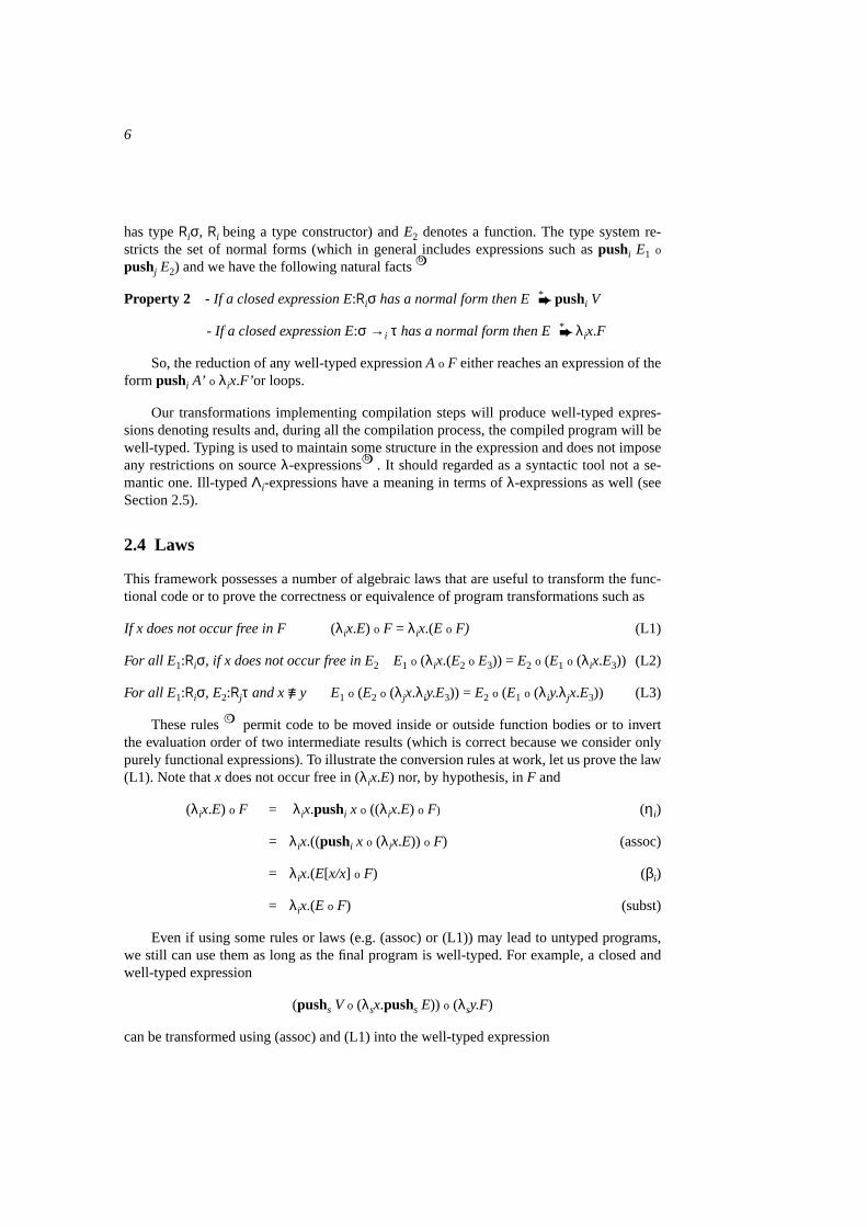
2.4 Laws

This framework possesses a number of algebraic laws that are useful to transform the func-tional code or to prove the correctness or equivalence of program transformations such as

If x does not occur free in F (λix.E) o F = λix.(E o F) (L1)

For all E1:Riσ, if x does not occur free in E2 E1 o (λix.(E2 o E3)) = E2 o (E1 o (λix.E3)) (L2)

For all E1:Riσ, E2:Rjτ and x≡/ y E1 o (E2 o (λjx.λiy.E3)) = E2 o (E1 o (λiy.λjx.E3)) (L3)

These rulesc

permit code to be moved inside or outside function bodies or to invertthe evaluation order of two intermediate results (which is correct because we consider onlypurely functional expressions). To illustrate the conversion rules at work, let us prove the law(L1). Note thatx does not occur free in (λix.E) nor, by hypothesis, inF and

(λix.E) o F = λix.pushi x o ((λix.E) o F) (ηi)

= λix.((pushi x o (λix.E)) o F) (assoc)

= λix.(E[x/x] o F) (βi)

= λix.(E o F) (subst)

Even if using some rules or laws (e.g. (assoc) or (L1)) may lead to untyped programs,we still can use them as long as the final program is well-typed. For example, a closed andwell-typed expression

(pushs V o (λsx.pushs E)) o (λsy.F)

can be transformed using (assoc) and (L1) into the well-typed expression

7

pushs V o λsx.(pushs E o (λsy.F))

To simplify the presentation, we often omit parentheses and write for examplepushi E o

λix.F o G for (pushi E) o (λix.(F o G)). We also use syntactic sugar such as tuples (x1,…,xn)and simple pattern-matchingλi(x1,…,xn).E.

2.5 Instantiation

The intermediate languagesΛi are subsets of theλ-calculus made of combinators. An impor-tant point is that we do not have to give a precise definition to combinators. We just assumethat they respect properties (βi), (ηi) and (assoc). Definitions can be chosen only after the lastcompilation step. This feature allows us to shift from theβi-reduction inΛi to a state-ma-chine-like expression reduction. Moreover, it permits to specify the implementation of com-ponents independently from the other steps. For example, we may eventually choose toimplement the data components and the environment componente either as a single stack oras two separate ones. We present in Section 7 an example of instantiation for the Cam.

In order to provide some intuition, we nevertheless give here some possible definitionsin terms of standardλ-expressions. The most natural definition for the sequencing combina-tor is o = λabc.a (b c), that isE1 o E2 = λc.E1 (E2 c). The (fresh) variablec can be seen as acontinuation and implements the sequencing.

The pairs of combinators (λi, pushi) can be seen as encoding a component of an under-lying abstract machine and their definitions as specifying the state transitions. A sequence ofcode such aspushi E1 o … o pushi En o … suggests that the underlying machine must pos-sess a componenti (such as a stack, a list, a tree or a vector) in order to store intermediate re-sults. We can choose to keep the components separate or merge (some of) them.

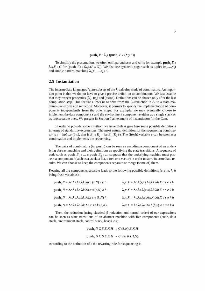
Keeping all the components separate leads to the following possible definitions (c, s, e, k, hbeing fresh variables):

pushsN = λc.λs.λe.λk.λh.c (s,N) e k h λsx.X = λc.λ(s,x).λe.λk.λh.X c s e k h

pusheN = λc.λs.λe.λk.λh.c s(e,N) k h λex.X = λc.λs.λ(e,x).λk.λh.X c s e k h

pushk N = λc.λs.λe.λk.λh.c s e(k,N) h λkx.X = λc.λs.λe.λ(k,x).λh.X c s e k h

pushh N = λc.λs.λe.λk.λh.c s e k(h,N) λhx.X = λc.λs.λe.λk.λ(h,x).X c s e k h

Then, the reduction (using classicalβ-reduction and normal order) of our expressionscan be seen as state transitions of an abstract machine with five components (code, datastack, environment stack, control stack, heap), e.g.:

pushs N C S E K H→ C (S,N) E K H

pushh N C S E K H→ C S E K (H,N)

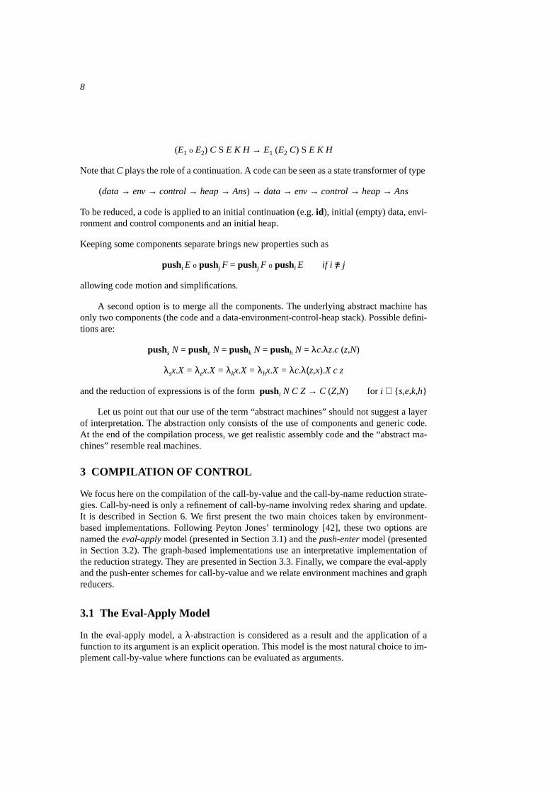
According to the definition ofo the rewriting rule for sequencing is

8

(E1 o E2) C S E K H → E1 (E2 C) S E K H

Note thatC plays the role of a continuation. A code can be seen as a state transformer of type

(data→ env→ control→ heap→ Ans) → data→ env→ control→ heap→ Ans

To be reduced, a code is applied to an initial continuation (e.g.id), initial (empty) data, envi-ronment and control components and an initial heap.

Keeping some components separate brings new properties such as

pushi E o pushj F = pushj F o pushi E if i ≡/ j

allowing code motion and simplifications.

A second option is to merge all the components. The underlying abstract machine hasonly two components (the code and a data-environment-control-heap stack). Possible defini-tions are:

pushs N = pushe N = pushk N = pushh N = λc.λz.c (z,N)

λsx.X = λex.X = λkx.X = λhx.X = λc.λ(z,x).X c z

and the reduction of expressions is of the formpushi N C Z→ C (Z,N) for i ∈ s,e,k,h

Let us point out that our use of the term “abstract machines” should not suggest a layerof interpretation. The abstraction only consists of the use of components and generic code.At the end of the compilation process, we get realistic assembly code and the “abstract ma-chines” resemble real machines.

3 COMPILATION OF CONTROL

We focus here on the compilation of the call-by-value and the call-by-name reduction strate-gies. Call-by-need is only a refinement of call-by-name involving redex sharing and update.It is described in Section 6. We first present the two main choices taken by environment-based implementations. Following Peyton Jones’ terminology [42], these two options arenamed theeval-apply model (presented in Section 3.1) and thepush-enter model (presentedin Section 3.2). The graph-based implementations use an interpretative implementation ofthe reduction strategy. They are presented in Section 3.3. Finally, we compare the eval-applyand the push-enter schemes for call-by-value and we relate environment machines and graphreducers.

3.1 The Eval-Apply Model

In the eval-apply model, aλ-abstraction is considered as a result and the application of afunction to its argument is an explicit operation. This model is the most natural choice to im-plement call-by-value where functions can be evaluated as arguments.

9

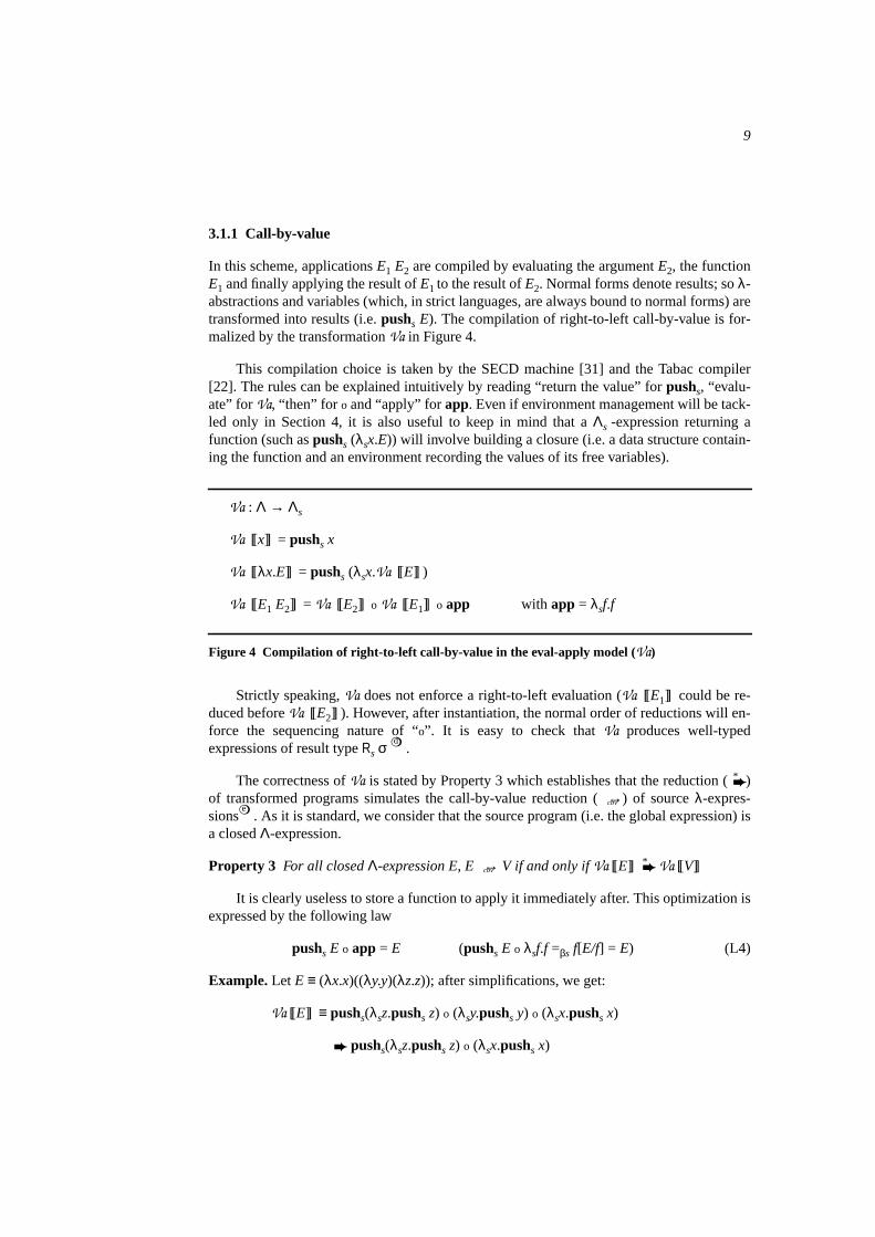
3.1.1 Call-by-value

In this scheme, applicationsE1 E2 are compiled by evaluating the argumentE2, the functionE1 and finally applying the result ofE1 to the result ofE2. Normal forms denote results; soλ-abstractions and variables (which, in strict languages, are always bound to normal forms) aretransformed into results (i.e.pushs E). The compilation of right-to-left call-by-value is for-malized by the transformationVa in Figure 4.

This compilation choice is taken by the SECD machine [31] and the Tabac compiler[22]. The rules can be explained intuitively by reading “return the value” forpushs, “evalu-ate” forVa, “then” for o and “apply” forapp. Even if environment management will be tack-led only in Section 4, it is also useful to keep in mind that aΛs -expression returning afunction (such aspushs (λsx.E)) will involve building a closure (i.e. a data structure contain-ing the function and an environment recording the values of its free variables).

Va : Λ → Λs

Va [[x]] = pushs x

Va [[λx.E]] = pushs (λsx.Va [[E]] )

Va [[E1 E2]] = Va [[E2]] o Va [[E1]] o app with app = λsf.f

Figure 4 Compilation of right-to-left call-by-value in the eval-apply model (Va)

Strictly speaking,Va does not enforce a right-to-left evaluation (Va [[E1]] could be re-duced beforeVa [[E2]] ). However, after instantiation, the normal order of reductions will en-force the sequencing nature of “o”. It is easy to check thatVa produces well-typedexpressions of result typeRs σ d .

The correctness ofVa is stated by Property 3 which establishes that the reduction (*)

of transformed programs simulates the call-by-value reduction (cbv→) of sourceλ-expres-sions

e. As it is standard, we consider that the source program (i.e. the global expression) is

a closedΛ-expression.

Property 3 For all closedΛ-expression E, Ecbv→ V if and only ifVa [[E]] * Va [[V]]

It is clearly useless to store a function to apply it immediately after. This optimization isexpressed by the following law

pushs E o app = E (pushs E o λsf.f =βs f[E/f] = E) (L4)

Example. Let E ≡ (λx.x)((λy.y)(λz.z)); after simplifications, we get:

Va [[E]] ≡ pushs(λsz.pushs z) o (λsy.pushs y) o (λsx.pushs x)

pushs(λsz.pushs z) o (λsx.pushs x)

10

pushs(λsz.pushs z) ≡ Va [[λz.z]]

The source expression has two redexes (λx.x)((λy.y)(λz.z)) and (λy.y)(λz.z) but only the lattercan be chosen by a call-by-value strategy. In contrast,Va [[E]] has only the compiled versionof (λy.y)(λz.z) as redex. The illicit (in call-by-value) reductionE → (λy.y)(λz.z) cannot occurwithin Va [[E]] . This illustrates the fact that the reduction strategy has been compiled andthat the choice of redex inΛs is not semantically relevant.

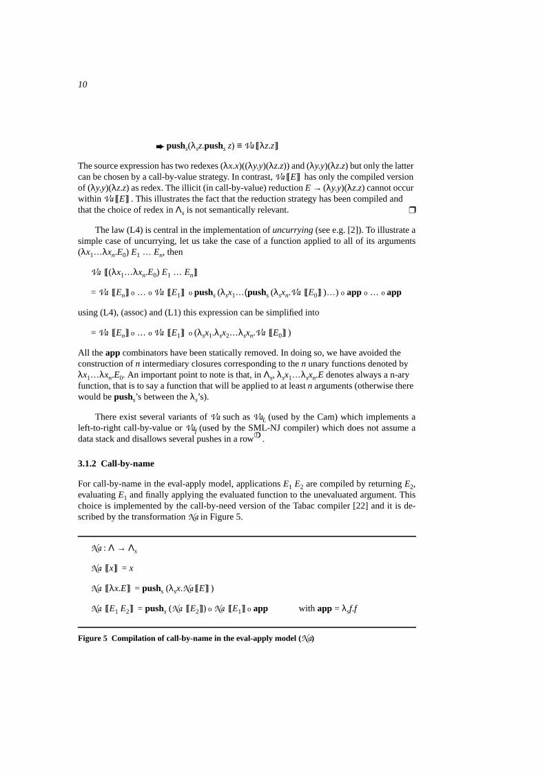
The law (L4) is central in the implementation ofuncurrying (see e.g. [2]). To illustrate asimple case of uncurrying, let us take the case of a function applied to all of its arguments(λx1…λxn.E0) E1 … En, then

Va [[(λx1…λxn.E0) E1 … En]]

= Va [[En]] o … o Va [[E1]] o pushs (λsx1…(pushs (λsxn.Va [[E0]] )…) o app o … o app

using (L4), (assoc) and (L1) this expression can be simplified into

= Va [[En]] o … o Va [[E1]] o (λsx1.λsx2…λsxn.Va [[E0]] )

All the app combinators have been statically removed. In doing so, we have avoided theconstruction ofn intermediary closures corresponding to then unary functions denoted byλx1…λxn.E0. An important point to note is that, inΛs, λsx1…λsxn.E denotes always a n-aryfunction, that is to say a function that will be applied to at leastn arguments (otherwise therewould bepushs’s between theλs’s).

There exist several variants ofVa such asVaL (used by the Cam) which implements aleft-to-right call-by-value orVaf (used by the SML-NJ compiler) which does not assume adata stack and disallows several pushes in a rowf .

3.1.2 Call-by-name

For call-by-name in the eval-apply model, applicationsE1 E2 are compiled by returningE2,evaluatingE1 and finally applying the evaluated function to the unevaluated argument. Thischoice is implemented by the call-by-need version of the Tabac compiler [22] and it is de-scribed by the transformationNa in Figure 5.

Na : Λ → Λs

Na [[x]] = x

Na [[λx.E]] = pushs (λsx.Na [[E]] )

Na [[E1 E2]] = pushs (Na [[E2]]) o Na [[E1]] o app with app = λsf.f

Figure 5 Compilation of call-by-name in the eval-apply model (Na)

11

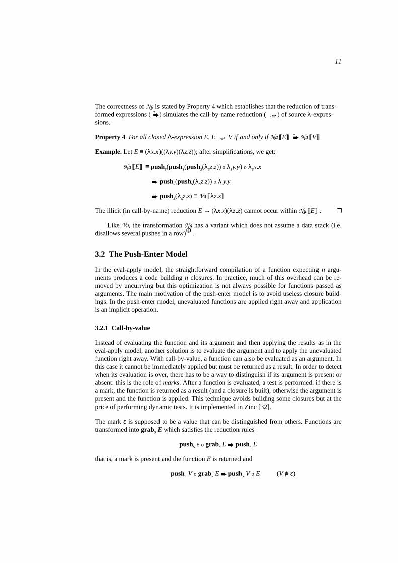
The correctness ofNa is stated by Property 4 which establishes that the reduction of trans-formed expressions (*) simulates the call-by-name reduction (cbn→) of sourceλ-expres-sions.

Property 4 For all closedΛ-expression E, Ecbn→ V if and only ifNa [[E]] * Na [[V]]

Example. Let E ≡ (λx.x)((λy.y)(λz.z)); after simplifications, we get:

Na [[E]] ≡ pushs(pushs(pushs(λsz.z)) o λsy.y) o λsx.x

pushs(pushs(λsz.z)) o λsy.y

pushs(λsz.z) ≡ Va [[λz.z]]

The illicit (in call-by-name) reductionE → (λx.x)(λz.z) cannot occur withinNa [[E]] .

Like Va, the transformationNa has a variant which does not assume a data stack (i.e.disallows several pushes in a row)g .

3.2 The Push-Enter Model

In the eval-apply model, the straightforward compilation of a function expectingn argu-ments produces a code buildingn closures. In practice, much of this overhead can be re-moved by uncurrying but this optimization is not always possible for functions passed asarguments. The main motivation of the push-enter model is to avoid useless closure build-ings. In the push-enter model, unevaluated functions are applied right away and applicationis an implicit operation.

3.2.1 Call-by-value

Instead of evaluating the function and its argument and then applying the results as in theeval-apply model, another solution is to evaluate the argument and to apply the unevaluatedfunction right away. With call-by-value, a function can also be evaluated as an argument. Inthis case it cannot be immediately applied but must be returned as a result. In order to detectwhen its evaluation is over, there has to be a way to distinguish if its argument is present orabsent: this is the role ofmarks. After a function is evaluated, a test is performed: if there isa mark, the function is returned as a result (and a closure is built), otherwise the argument ispresent and the function is applied. This technique avoids building some closures but at theprice of performing dynamic tests. It is implemented in Zinc [32].

The markε is supposed to be a value that can be distinguished from others. Functions aretransformed intograbs E which satisfies the reduction rules

pushs ε o grabs E pushs E

that is, a mark is present and the functionE is returned and

pushs V o grabs E pushs V o E (V ≡/ ε)

12

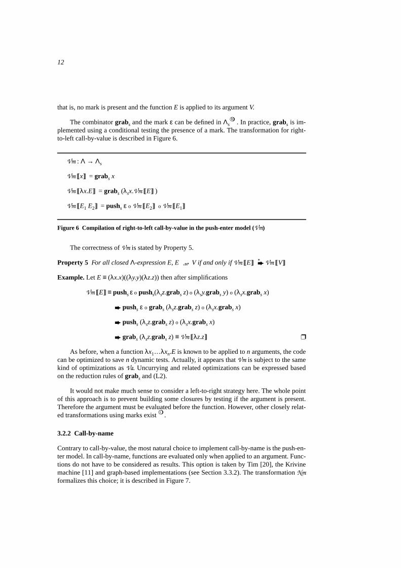
that is, no mark is present and the functionE is applied to its argumentV.

The combinatorgrabs and the markε can be defined inΛsh . In practice,grabs is im-

plemented using a conditional testing the presence of a mark. The transformation for right-to-left call-by-value is described in Figure 6.

Vm : Λ → Λs

Vm [[x]] = grabs x

Vm [[λx.E]] = grabs (λsx.Vm [[E]] )

Vm [[E1 E2]] = pushs ε o Vm [[E2]] o Vm [[E1]]

Figure 6 Compilation of right-to-left call-by-value in the push-enter model (Vm)

The correctness ofVm is stated by Property 5.

Property 5 For all closedΛ-expression E, Ecbv→ V if and only ifVm [[E]] * Vm [[V]]

Example. Let E ≡ (λx.x)((λy.y)(λz.z)) then after simplifications

Vm [[E]] ≡ pushsε o pushs(λsz.grabs z) o (λsy.grabs y) o (λsx.grabs x)

pushs ε o grabs (λsz.grabs z) o (λsx.grabs x)

pushs (λsz.grabs z) o (λsx.grabs x)

grabs (λsz.grabs z) ≡ Vm [[λz.z]]

As before, when a functionλx1…λxn.E is known to be applied ton arguments, the codecan be optimized to saven dynamic tests. Actually, it appears thatVm is subject to the samekind of optimizations asVa. Uncurrying and related optimizations can be expressed basedon the reduction rules ofgrabs and (L2).

It would not make much sense to consider a left-to-right strategy here. The whole pointof this approach is to prevent building some closures by testing if the argument is present.Therefore the argument must be evaluated before the function. However, other closely relat-ed transformations using marks existi .

3.2.2 Call-by-name

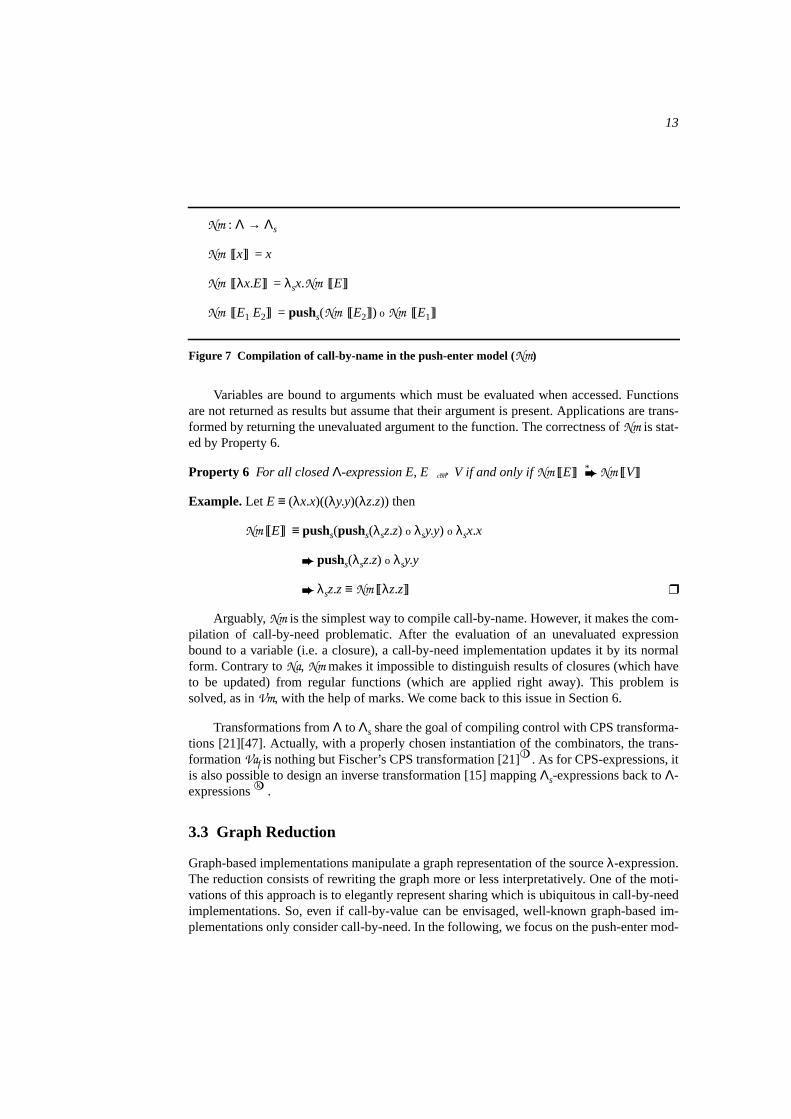
Contrary to call-by-value, the most natural choice to implement call-by-name is the push-en-ter model. In call-by-name, functions are evaluated only when applied to an argument. Func-tions do not have to be considered as results. This option is taken by Tim [20], the Krivinemachine [11] and graph-based implementations (see Section 3.3.2). The transformationNmformalizes this choice; it is described in Figure 7.

13

Nm : Λ → Λs

Nm [[x]] = x

Nm [[λx.E]] = λsx.Nm [[E]]

Nm [[E1 E2]] = pushs(Nm [[E2]]) o Nm [[E1]]

Figure 7 Compilation of call-by-name in the push-enter model (Nm)

Variables are bound to arguments which must be evaluated when accessed. Functionsare not returned as results but assume that their argument is present. Applications are trans-formed by returning the unevaluated argument to the function. The correctness ofNm is stat-ed by Property 6.

Property 6 For all closedΛ-expression E, Ecbn→ V if and only ifNm [[E]] * Nm [[V]]

Example. Let E ≡ (λx.x)((λy.y)(λz.z)) then

Nm [[E]] ≡ pushs(pushs(λsz.z) o λsy.y) o λsx.x

pushs(λsz.z) o λsy.y

λsz.z ≡ Nm [[λz.z]]

Arguably,Nm is the simplest way to compile call-by-name. However, it makes the com-pilation of call-by-need problematic. After the evaluation of an unevaluated expressionbound to a variable (i.e. a closure), a call-by-need implementation updates it by its normalform. Contrary toNa, Nm makes it impossible to distinguish results of closures (which haveto be updated) from regular functions (which are applied right away). This problem issolved, as inVm, with the help of marks. We come back to this issue in Section 6.

Transformations fromΛ to Λs share the goal of compiling control with CPS transforma-tions [21][47]. Actually, with a properly chosen instantiation of the combinators, the trans-formationVaf is nothing but Fischer’s CPS transformation [21]j . As for CPS-expressions, itis also possible to design an inverse transformation [15] mappingΛs-expressions back toΛ-expressions

k.

3.3 Graph Reduction

Graph-based implementations manipulate a graph representation of the sourceλ-expression.The reduction consists of rewriting the graph more or less interpretatively. One of the moti-vations of this approach is to elegantly represent sharing which is ubiquitous in call-by-needimplementations. So, even if call-by-value can be envisaged, well-known graph-based im-plementations only consider call-by-need. In the following, we focus on the push-enter mod-

14

el for call-by-name which is largely adopted by existing graph reducers. Its refinement intocall-by-need is presented in Section 6.2.2.

3.3.1 Graph building

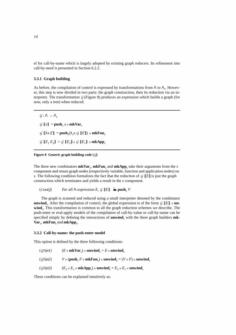
As before, the compilation of control is expressed by transformations fromΛ to Λs. Howev-er, this step is now divided in two parts: the graph construction, then its reduction via an in-terpreter. The transformationG (Figure 8) produces an expression which builds a graph (fornow, only a tree) when reduced.

G : Λ → Λs

G [[x]] = pushs x o mkVar s

G [[λx.E]] = pushs(λsx.G [[E]]) o mkFuns

G [[E1 E2]] = G [[E2]] o G [[E1]] o mkApp s

Figure 8 Generic graph building code (G)

The three new combinatorsmkVar s, mkFuns andmkApp s take their arguments from thescomponent and return graph nodes (respectively variable, function and application nodes) ons. The following condition formalizes the fact that the reduction ofG [[E]] is just the graphconstruction which terminates and yields a result in thes component.

(CondG) For all Λ-expression E, G [[E]] * pushs V

The graph is scanned and reduced using a small interpreter denoted by the combinatorunwinds. After the compilation of control, the global expression is of the formG [[E]] o un-winds. This transformation is common to all the graph reduction schemes we describe. Thepush-enter or eval-apply models of the compilation of call-by-value or call-by-name can bespecified simply by defining the interactions ofunwinds with the three graph buildersmk-Vars, mkFunsandmkApp s.

3.3.2 Call-by-name: the push-enter model

This option is defined by the three following conditions:

(GNm1) (E o mkVar s) o unwinds = E o unwinds

(GNm2) V o (pushs F o mkFuns) o unwinds = (V o F) o unwinds

(GNm3) (E2 o E1 o mkApp s) o unwinds = E2 o E1 o unwinds

These conditions can be explained intuitively as:

15

• (GNm1) The reduction of a variable node amounts to reducing the graph which has beenbound to the variable. The combinatormkVar s may seem useless since it is bypassed byunwinds. However, when call-by-need is considered,mkVar s is needed to implementupdating without losing sharing properties. As the combinatorI in [53], it represents in-direction nodes.

• (GNm2) The reduction of a function node amounts to applying the function to its argu-ment and to reducing the resulting graph. This rule makes the push-enter model clear.The reduction of the function node does not return the functionF as a result, but immedi-ately applies it.

• (GNm3) The reduction of an application node amounts to storing the argument graph andto reducing the function graph.

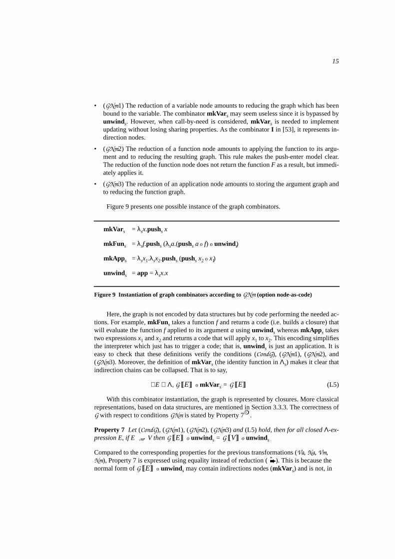
Figure 9 presents one possible instance of the graph combinators.

mkVar s = λsx.pushs x

mkFuns = λsf.pushs (λsa.(pushs a o f) o unwinds)

mkApp s = λsx1.λsx2.pushs (pushs x2 o x1)

unwinds = app = λsx.x

Figure 9 Instantiation of graph combinators according toGNm (option node-as-code)

Here, the graph is not encoded by data structures but by code performing the needed ac-tions. For example,mkFuns takes a functionf and returns a code (i.e. builds a closure) thatwill evaluate the functionf applied to its argumenta usingunwinds whereasmkApp s takestwo expressionsx1 andx2 and returns a code that will applyx1 to x2. This encoding simplifiesthe interpreter which just has to trigger a code; that is,unwinds is just an application. It iseasy to check that these definitions verify the conditions (CondG), (GNm1), (GNm2), and(GNm3). Moreover, the definition ofmkVar s (the identity function inΛs) makes it clear thatindirection chains can be collapsed. That is to say,

∀E ∈ Λ, G [[E]] o mkVar s = G [[E]] (L5)

With this combinator instantiation, the graph is represented by closures. More classicalrepresentations, based on data structures, are mentioned in Section 3.3.3. The correctness ofG with respect to conditionsGNm is stated by Property 7l .

Property 7 Let (CondG), (GNm1), (GNm2), (GNm3) and (L5) hold, then for all closedΛ-ex-pression E, if E cbn→ V thenG [[E]] o unwinds = G [[V]] o unwinds

Compared to the corresponding properties for the previous transformations (Va, Na, Vm,Nm), Property 7 is expressed using equality instead of reduction (*

). This is because thenormal form ofG [[E]] o unwinds may contain indirections nodes (mkVar s) and is not, in

16

general, syntactically identical toG [[V]] o unwinds. Actually,G verifies a stronger (but lesseasily formalized) property than Property 7:G [[E]] o unwinds reduces to an expressionXwhich, after removal of indirection chains, is syntactically equal to the graph ofG [[V]] .

Example. Let E ≡ (λx.x)((λy.y)(λz.z)) and

Iw ≡ (λsa. (pushs a o (λsw.pushs w o mkVar s)) o unwinds) then

G [[E]] o unwinds ≡ (G [[λz.z]] o G [[λy.y]] o mkApp s) o G [[λx.x]] o mkApp so unwinds

* pushs(pushs(pushs Iz o Iy) o Ix) o unwinds

pushs(pushs Iz o Iy) o (λsa. (pushs a o (λsx.pushs x o mkVar s)) o unwinds)

* pushs (pushs Iz o Iy) o unwinds

pushs Izo (λsa. (pushs a o (λsy.pushs y o mkVar s)) o unwinds)

* (pushs Izo mkVar s) o unwinds pushs Izo unwinds

In this example, there is no indirection chain and the result is syntactically equal to the graphof the source normal form. That is,pushs Izo unwinds is exactlyG [[λz.z]] o unwinds after thefew reductions corresponding to graph construction.

The first sequence of reductions corresponds to the graph construction. Thenunwinds scansthe (leftmost) spine (the firstpushs represents an application node). The graph representingthe function (λx.x) is applied. The result is the application nodepushs (pushs Iz o Iy) which isscanned byunwinds. Then, the reduction proceeds in the same way until it reaches the nor-mal form.

Because of the interpretative essence of the graph reduction, a naive implementation ofcall-by-need is possible without introducing marks (as opposed toNm in Section 3.2.2).Such a scheme performs many useless updates some of which can be detected by simplesyntactic criteria or a sharing analysis. An optimized implementation, performing selectiveupdates, can be defined by introducing marks. These two points are presented in Section6.2.2.

3.3.3 Other choices

A graph and its associated reducer can be seen as an abstract data type with different imple-mentations [41]. We have already used one encoding that represents nodes by code (i.e. clo-sures). Another natural solution is to represent the graph by a data structure. It amounts tointroducing three data constructorsVarNode, FunNode andAppNode and to defining theinterpreterunwinds by a case expression. A refinement, exploited by the G-machine, is toenclose in nodes the code to be executed when it is unwound. Adding code in data structurescomes very close to the solution using closures described in Figure 9. The interpreterun-winds can just execute the code and does not have to perform a dynamic test. In any case, thenew combinator definitions should still verify theGNm properties in order to implement apush-enter model of the compilation of call-by-name.

17

By far, the most common use of graph reduction is the implementation of call-by-needin the push-enter model. However, the eval-apply model or the compilation of call-by-valuecan be expressed as well. These choices are specified by redefining the interactions ofun-winds with the three graph builders (mkVar s, mkFuns, mkApp s). In each case, it amountsto defining new properties like (GNm1), (GNm2), and (GNm3).

More details on these alternate choices can be found in [18].

3.4 Comparisons

We compare the efficiency of codes produced by transformationsVa (eval-apply CBV) andVm (push-enter CBV). Then, we exhibit the precise relationship between the environmentand graph approaches. In particular, it is shown how to derive the transformationNm from Gand the properties (GNmi). We take only these two examples to show the advantages of a uni-fied framework in terms of formal comparisons. It should be clear that such comparisonscould be carried on for other transformations and compilation steps.

3.4.1 Va versusVm

Let us first emphasize that our comparisons focus on finding complexity upper bounds. Theydo not take the place of benchmarks which are still required to take into account compleximplementation aspects (e.g. interactions with memory cache or the garbage collector).

A code produced byVm builds less closures than the correspondingVa-code. Since amark can be represented by one bit (e.g. in a bit stack parallel to the data stack),Vm is likelyto be, on average, more efficient with respect to space resources. Concerning time efficiency,the size of compiled expressions provides a first approximation of the cost entailed by theencoding of the reduction strategy (assumingpushs, grabs andapp have a constant time im-plementation). It is easy to show that code expansion is linear with respect to the size of thesource expression. More precisely, forVx = Va or Vm, we have

If Size (E) = n thenSize (Vx [[E]]) < 3n.

This upper bound can be reached by taking for exampleE ≡ λx.x … x (n occurrences ofx). A more thorough investigation is possible by associating costs with the different combi-nators encoding the control:push for the cost of “pushing” a variable or a mark,clos for thecost of building a closure (i.e.pushs E), app andgrab for the cost of the corresponding com-binators. If we takenλ for the number ofλ-abstractions andnv for the number of occurrencesof variables in the source expression, we have

Cost (Va [[E]]) = nλ clos + nv push + (nv-1) app

and Cost (Vm [[E]]) = (nλ + nv) grab+ (nv-1) push

The benefit ofVm overVa is to sometimes replace a (useless) closure construction by atest. When a closure has to be built,Vm involves a useless test compared toVa. So ifclos iscomparable to the cost of a test (for example, when returning a closure amounts to building a

18

pair as in Section 4.1.2)Vm will produce more expensive code thanVa. If closure building isnot a constant time operation (as in Section 4.1.3)Vm can be arbitrarily better thanVa. Actu-ally, it can change the program complexity in contrived cases. In practice, however, the situ-ation is not so clear. When no mark is present,grabs is implemented by a test followed by anapp. If a mark is present, the test is followed by apushs (i.e. a closure building forλ-ab-stractions). So, we have

Cost (Vm [[E]]) = (nλ+nv) test+ p (nλ+nv) app + p nλ clos+ p nv push + (nv-1) push

with p (resp.p) representing the likelihood (p+p=1) of the presence (resp. absence) of amark which depends on the program. The best situation forVm is when no closure has to bebuilt, that isp=0 andp=1. If we take some reasonable hypothesis such astest=app andnλ <nv<3nλ, we find that the cost of closure construction must be 3 to 5 times more costlythanappor test to makeVm advantageous. With less favorable odds such asp=p=1/2, closmust be worth 7 or 8app.

We are led to conclude thatVm should be considered only when closure building is po-tentially costly (such as theAc2 transformation in Section 4.1.3 which builds closures bycopying part of the environment). Even so, tests may be too costly in practice compared tothe construction of small closures. The best way would probably be to perform an analysis todetect cases whenVm is profitable. Such information could be taken into account to get thebest of each approach. We present in [17] howVa andVm could be mixed.

3.4.2 Environment machineversus graph reducer

Even if their starting points are utterly different, graph reducers and environment machinescan be related. This has been done for specific implementations such as [43] which showshow to transform a G-machine into a Tim. We focus here on the compilation of control andcompare the transformationNm with theGNm approach to graph reduction.

The two main departures of graph reduction from the environment approach are

• The potentially useless graph constructions. For example, the ruleG [[E1 E2]] = G[[E2]] o G [[E1]] o mkApps builds a graph forE2 even ifE2 is never reduced (i.e. if it isnot needed). On the other hand,Nm suspends all operations (such as variable instantia-tion) onE2 by building a closure (Nm [[E1 E2]] = pushs (Nm [[E2]]) o Nm [[E1]] ).

• The interpretative nature of graph reduction. Even in the “node-as-code” instantiation,each application node (mkApps) is “interpreted” byunwinds. In the environment family,no interpreter is needed and this approach can be seen as the specialization of the inter-preterunwinds according to the source graph built byG [[]] .

In order to formalize these two points, we first change the rule for graph building in thecase of applications by

G [[E1 E2]] = pushs (G [[E2]] o unwinds) o G [[E1]] o mkApp s

19

This corresponds to a lazy graph construction where the graph argument is built only ifneeded. In particular, variables will be bound to unbuilt graphs. This new kind of graph en-tails replacing property (GNm1) with

(GNm1) (pushs E o mkVar s) o unwinds = E

We can now show thatNm [[E]] is merely the specialization ofunwinds with respect to thegraph ofE; that is

Nm [[E]] = G [[E]] o unwinds

For example, the specialization for the application case is:

G [[E1 E2]] o unwinds

= pushs(G [[E2]] o unwinds) o G [[E1]] o mkApp s o unwinds (unfoldingG)

= pushs (G [[E2]] o unwinds) o G [[E1]] o unwinds (GNm3)

= pushs (Nm [[E2]]) o Nm [[E1]] (induction hypothesis)

= Nm [[E1 E2]] (folding N)

This property shows that, as far as the compilation of control is concerned, environmentbased transformations are more efficient than their graph counterpart. However, optimizedgraph reducers avoid as much as possible interpretative scans of the graph or graph buildingand are similar to environment-based implementations.

4 COMPILATION OF THE β-REDUCTION

This compilation step implements the substitution using transformations fromΛs to Λe.These transformations are akin to abstraction algorithms and consist of replacing variableswith combinators. Compared toΛs, Λe adds the pair (pushe, λe) encoding an environmentcomponent and it uses variables only to define combinators. Graph reducers use specific(usually environment-less) transformations. We express in our framework theSKI abstrac-tion algorithm (Section 4.2).

4.1 Environment Based Abstractions

In theλ-calculus, theβ-reduction is defined as a textual substitution. In environment-basedimplementations, substitutions are compiled by storing the value to be substituted in a datastructure (an environment). Values are then accessed in the environment only when needed.This technique can be compared with the activation records used by imperative languagecompilers. The main choice is using list-like (shared) environments or vector-like (copied)environments. For the latter choice, there are several transformations depending when theenvironments are copied.

20

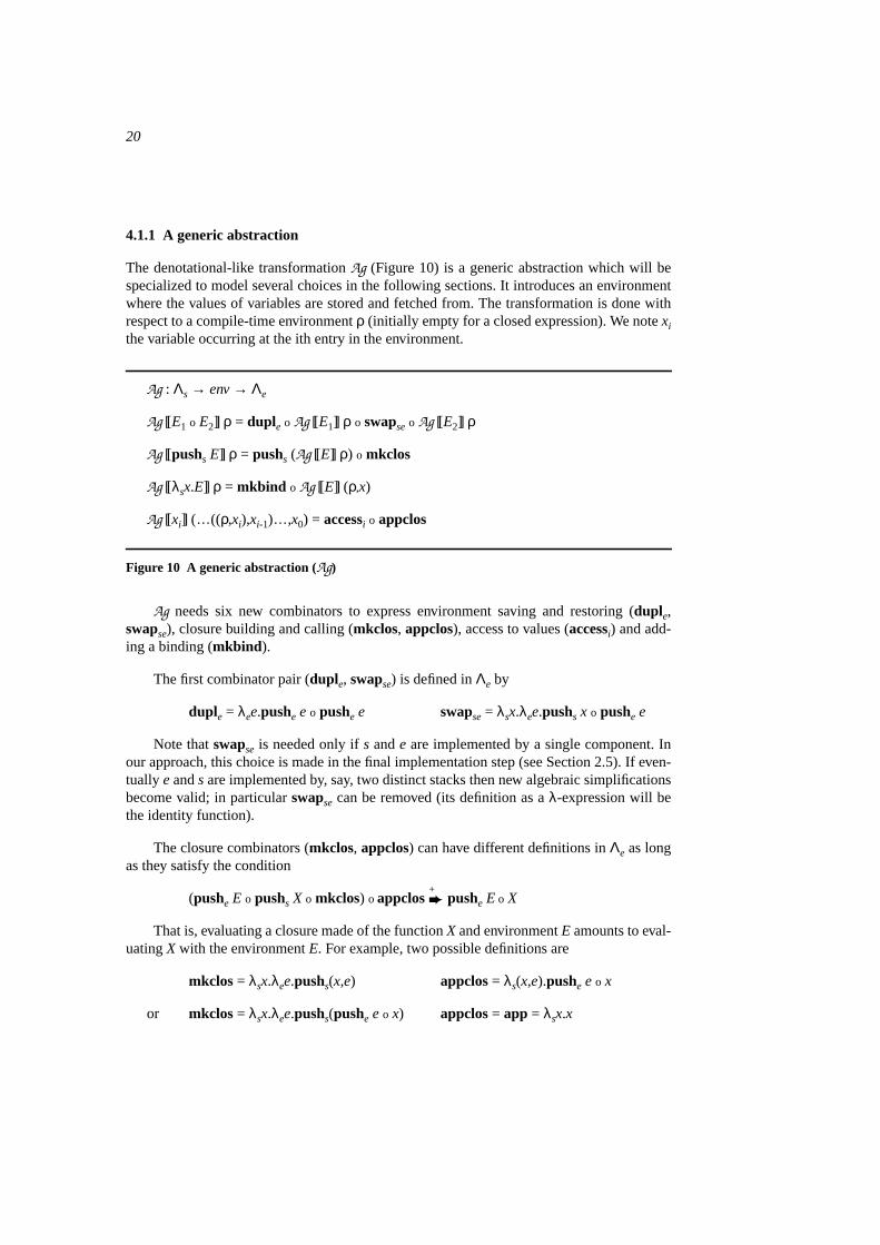
4.1.1 A generic abstraction

The denotational-like transformationAg (Figure 10) is a generic abstraction which will bespecialized to model several choices in the following sections. It introduces an environmentwhere the values of variables are stored and fetched from. The transformation is done withrespect to a compile-time environmentρ (initially empty for a closed expression). We notexithe variable occurring at the ith entry in the environment.

Ag : Λs → env→ Λe

Ag [[E1 o E2]] ρ = duple o Ag [[E1]] ρ o swapseo Ag [[E2]] ρ

Ag [[pushs E]] ρ = pushs (Ag [[E]] ρ) o mkclos

Ag [[λsx.E]] ρ = mkbind o Ag [[E]] (ρ,x)

Ag [[xi]] (…((ρ,xi),xi-1)…,x0) = accessi o appclos

Figure 10 A generic abstraction (Ag)

Ag needs six new combinators to express environment saving and restoring (duple,swapse), closure building and calling (mkclos, appclos), access to values (accessi) and add-ing a binding (mkbind ).

The first combinator pair (duple, swapse) is defined inΛe by

duple = λee.pushe e o pushe e swapse = λsx.λee.pushs x o pushe e

Note thatswapse is needed only ifs ande are implemented by a single component. Inour approach, this choice is made in the final implementation step (see Section 2.5). If even-tually e ands are implemented by, say, two distinct stacks then new algebraic simplificationsbecome valid; in particularswapse can be removed (its definition as aλ-expression will bethe identity function).

The closure combinators (mkclos, appclos) can have different definitions inΛe as longas they satisfy the condition

(pushe E o pushs X o mkclos) o appclos+

pushe E o X

That is, evaluating a closure made of the functionX and environmentE amounts to eval-uatingX with the environmentE. For example, two possible definitions are

mkclos = λsx.λee.pushs(x,e) appclos = λs(x,e).pushe e o x

or mkclos = λsx.λee.pushs(pushe e o x) appclos = app = λsx.x

21

The first option uses pairs and is, in a way, more concrete than the other one. The sec-ond option abstracts from representation considerations. It simplifies the expression of cor-rectness properties and it will be used in the rest of the paper.

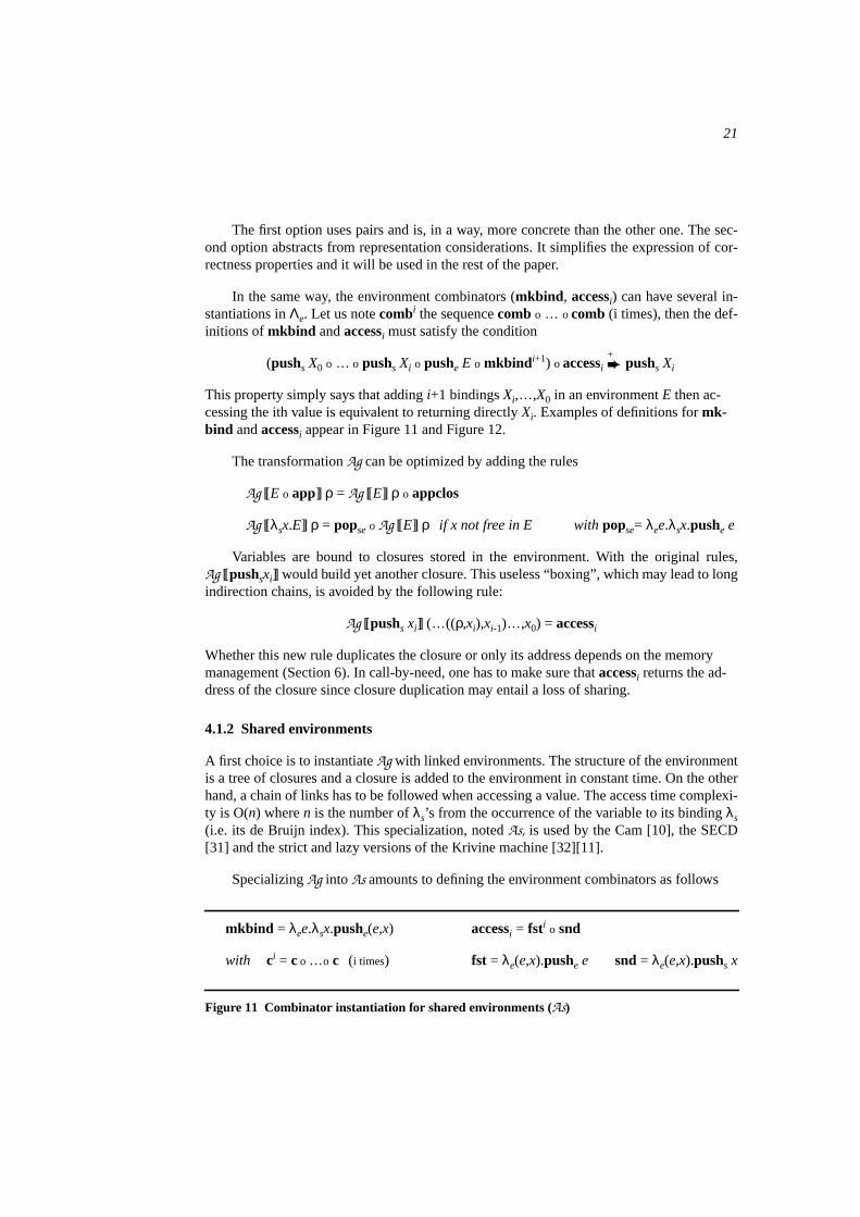
In the same way, the environment combinators (mkbind , accessi) can have several in-stantiations inΛe. Let us notecombi the sequencecomb o … o comb (i times), then the def-initions ofmkbind andaccessi must satisfy the condition

(pushs X0 o … o pushs Xi o pushe E o mkbind i+1) o accessi +

pushs Xi

This property simply says that addingi+1 bindingsXi,…,X0 in an environmentE then ac-cessing the ith value is equivalent to returning directlyXi. Examples of definitions formk-bind andaccessi appear in Figure 11 and Figure 12.

The transformationAg can be optimized by adding the rules

Ag [[E o app]] ρ = Ag [[E]] ρ o appclos

Ag [[λsx.E]] ρ = popseo Ag [[E]] ρ if x not free in E withpopse= λee.λsx.pushe e

Variables are bound to closures stored in the environment. With the original rules,Ag [[pushsxi]] would build yet another closure. This useless “boxing”, which may lead to longindirection chains, is avoided by the following rule:

Ag [[pushs xi]] (…((ρ,xi),xi-1)…,x0) = accessi

Whether this new rule duplicates the closure or only its address depends on the memorymanagement (Section 6). In call-by-need, one has to make sure thataccessi returns the ad-dress of the closure since closure duplication may entail a loss of sharing.

4.1.2 Shared environments

A first choice is to instantiateAg with linked environments. The structure of the environmentis a tree of closures and a closure is added to the environment in constant time. On the otherhand, a chain of links has to be followed when accessing a value. The access time complexi-ty is O(n) wheren is the number ofλs’s from the occurrence of the variable to its bindingλs(i.e. its de Bruijn index). This specialization, notedAs, is used by the Cam [10], the SECD[31] and the strict and lazy versions of the Krivine machine [32][11].

SpecializingAg into As amounts to defining the environment combinators as follows

mkbind = λee.λsx.pushe(e,x) accessi = fsti o snd

with ci = co …o c (i times) fst = λe(e,x).pushe e snd = λe(e,x).pushs x

Figure 11 Combinator instantiation for shared environments (As)

22

Example. As [[λsx1.λsx0.pushs E o x1]] ρ = mkbind o mkbind o duple o

pushs (As [[E]] ((ρ,x1),x0)) o mkclos o swapseo access1 o appclos

Two bindings are added (mkbind o mkbind ) to the current environment and thex1 access iscoded byaccess1 = fst o snd.

The correctness ofAs is stated by Property 8m

.

Property 8 For all closed well-typedΛs-expression E,pushe () o As [[E]] () = E

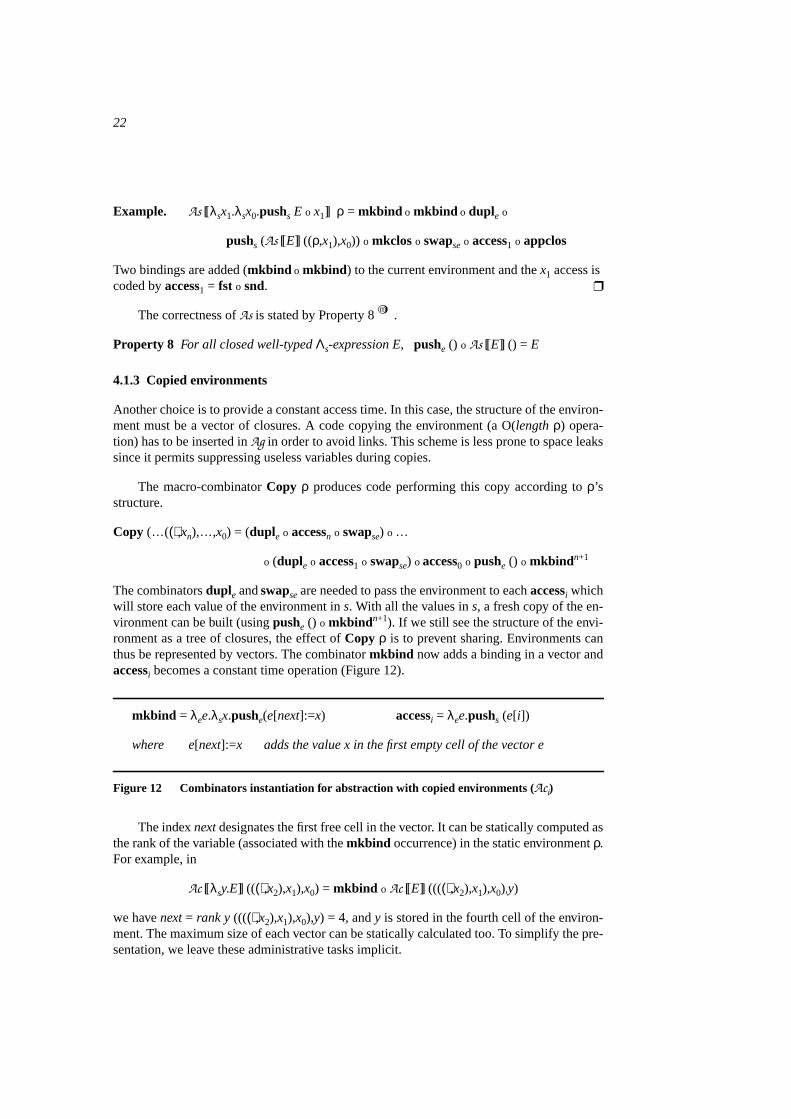
4.1.3 Copied environments

Another choice is to provide a constant access time. In this case, the structure of the environ-ment must be a vector of closures. A code copying the environment (a O(lengthρ) opera-tion) has to be inserted inAg in order to avoid links. This scheme is less prone to space leakssince it permits suppressing useless variables during copies.

The macro-combinatorCopy ρ produces code performing this copy according toρ’sstructure.

Copy (…((),xn),…,x0) = (duple o accessn o swapse) o …

o (duple o access1 o swapse) o access0 o pushe () o mkbindn+1

The combinatorsduple andswapse are needed to pass the environment to eachaccessi whichwill store each value of the environment ins. With all the values ins, a fresh copy of the en-vironment can be built (usingpushe () o mkbindn+1). If we still see the structure of the envi-ronment as a tree of closures, the effect ofCopy ρ is to prevent sharing. Environments canthus be represented by vectors. The combinatormkbind now adds a binding in a vector andaccessi becomes a constant time operation (Figure 12).

mkbind = λee.λsx.pushe(e[next]:=x) accessi = λee.pushs (e[i])

where e[next]:=x adds the value x in the first empty cell of the vector e

Figure 12 Combinators instantiation for abstraction with copied environments (Aci)

The indexnext designates the first free cell in the vector. It can be statically computed asthe rank of the variable (associated with themkbind occurrence) in the static environmentρ.For example, in

Ac [[λsy.E]] (( (),x2),x1),x0) = mkbind o Ac [[E]] ((( (),x2),x1),x0),y)

we havenext = rank y((((),x2),x1),x0),y) = 4, andy is stored in the fourth cell of the environ-ment. The maximum size of each vector can be statically calculated too. To simplify the pre-sentation, we leave these administrative tasks implicit.

23

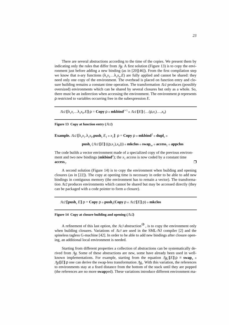
There are several abstractions according to the time of the copies. We present them byindicating only the rules that differ fromAg. A first solution (Figure 13) is to copy the envi-ronment just before adding a new binding (as in [20][46]). From the first compilation stepwe know that n-ary functions (λsx1…λsxn.E) are fully applied and cannot be shared: theyneed only one copy of the environment. The overhead is placed on function entry and clo-sure building remains a constant time operation. The transformationAc1 produces (possiblyoversized) environments which can be shared by several closures but only as a whole. So,there must be an indirection when accessing the environment. The environmentρ representsρ restricted to variables occurring free in the subexpressionE.

Ac1 [[λsxi…λsx0.E]] ρ = Copy ρ o mkbind i+ 1 o Ac1 [[E]] (…(ρ,xi)…,x0)

Figure 13 Copy at function entry (Ac1)

Example.Ac1 [[λsx1.λsx0.pushs E1 o x1]] ρ = Copy ρ o mkbind2 o duple o

pushs (Ac1 [[E]] ((ρ,x1),x0))) o mkclos o swapseo access1 o appclos

The code builds a vector environment made of a specialized copy of the previous environ-ment and two new bindings (mkbind2); thex1 access is now coded by a constant timeaccess1.

A second solution (Figure 14) is to copy the environment when building and openingclosures (as in [22]). The copy at opening time is necessary in order to be able to add newbindings in contiguous memory (the environment has to remain a vector). The transforma-tion Ac2 produces environments which cannot be shared but may be accessed directly (theycan be packaged with a code pointer to form a closure).

Ac2 [[pushs E]] ρ = Copy ρ o pushs(Copy ρ o Ac2 [[E]] ρ) o mkclos

Figure 14 Copy at closure building and opening (Ac2)

A refinement of this last option, theAc3 abstractionn

, is to copy the environment onlywhen building closures. Variations ofAc3 are used in the SML-NJ compiler [2] and thespineless tagless G-machine [42]. In order to be able to add new bindings after closure open-ing, an additional local environment is needed.

Starting from different properties a collection of abstractions can be systematically de-rived from Ag. Some of these abstractions are new, some have already been used in well-known implementations. For example, starting from the equationAgs [[E]] ρ = swapn o

Ag [[E]] ρ one can derive the swap-less transformationAgs. With this variation, the referencesto environments stay at a fixed distance from the bottom of the stack until they are popped(the references are no moreswapped). These variations introduce different environment ma-

24

nipulation schemes avoiding stacks elements reordering (swap-less), environment duplica-tion (dupl-less), environment building (mkbind-less) or closure building (mkclos-less)o .

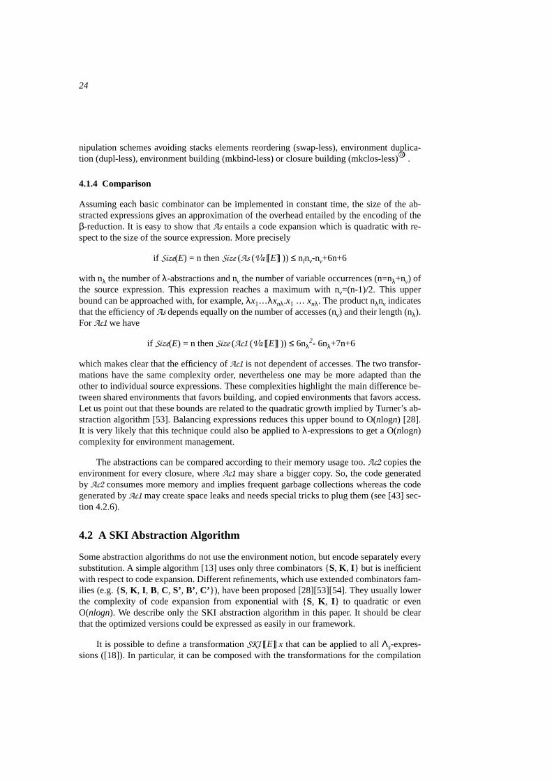
4.1.4 Comparison

Assuming each basic combinator can be implemented in constant time, the size of the ab-stracted expressions gives an approximation of the overhead entailed by the encoding of theβ-reduction. It is easy to show thatAs entails a code expansion which is quadratic with re-spect to the size of the source expression. More precisely

if Size(E) = n thenSize (As (Va [[E]] )) ≤ nlnv-nv+6n+6

with nλ the number ofλ-abstractions and nv the number of variable occurrences (n=nλ+nv) ofthe source expression. This expression reaches a maximum with nv=(n-1)/2. This upperbound can be approached with, for example,λx1…λxnλ.x1 … xnλ. The product nλnv indicatesthat the efficiency ofAs depends equally on the number of accesses (nv) and their length (nλ).For Ac1 we have

if Size(E) = n thenSize (Ac1 (Va [[E]] )) ≤ 6nλ2- 6nλ+7n+6

which makes clear that the efficiency ofAc1 is not dependent of accesses. The two transfor-mations have the same complexity order, nevertheless one may be more adapted than theother to individual source expressions. These complexities highlight the main difference be-tween shared environments that favors building, and copied environments that favors access.Let us point out that these bounds are related to the quadratic growth implied by Turner’s ab-straction algorithm [53]. Balancing expressions reduces this upper bound to O(nlogn) [28].It is very likely that this technique could also be applied toλ-expressions to get a O(nlogn)complexity for environment management.

The abstractions can be compared according to their memory usage too.Ac2 copies theenvironment for every closure, whereAc1 may share a bigger copy. So, the code generatedby Ac2 consumes more memory and implies frequent garbage collections whereas the codegenerated byAc1 may create space leaks and needs special tricks to plug them (see [43] sec-tion 4.2.6).

4.2 A SKI Abstraction Algorithm

Some abstraction algorithms do not use the environment notion, but encode separately everysubstitution. A simple algorithm [13] uses only three combinators S, K , I but is inefficientwith respect to code expansion. Different refinements, which use extended combinators fam-ilies (e.g. S, K , I , B, C, S’, B’ , C’ ), have been proposed [28][53][54]. They usually lowerthe complexity of code expansion from exponential with S, K , I to quadratic or evenO(nlogn). We describe only the SKI abstraction algorithm in this paper. It should be clearthat the optimized versions could be expressed as easily in our framework.

It is possible to define a transformationSKI [[E]] x that can be applied to allΛs-expres-sions ([18]). In particular, it can be composed with the transformations for the compilation

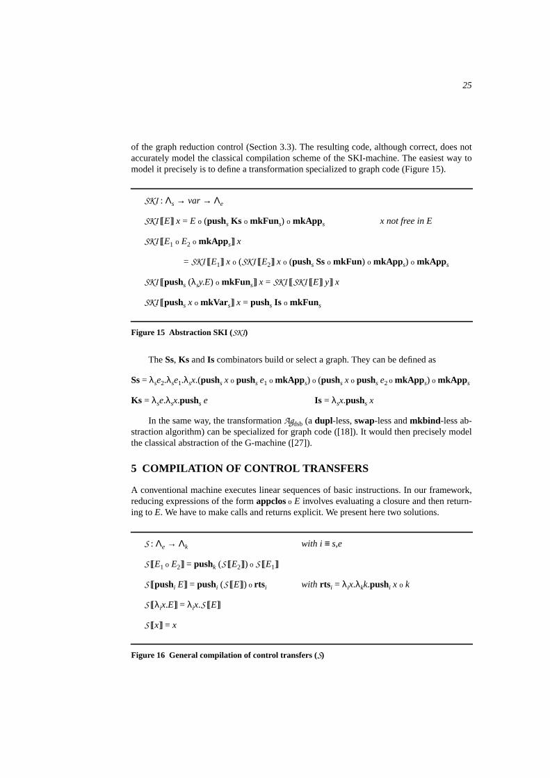
25

of the graph reduction control (Section 3.3). The resulting code, although correct, does notaccurately model the classical compilation scheme of the SKI-machine. The easiest way tomodel it precisely is to define a transformation specialized to graph code (Figure 15).

SKI : Λs → var → Λe

SKI [[E]] x = E o (pushs Ks o mkFuns) o mkApp s x not free in E

SKI [[E1 o E2 o mkApp s]] x

= SKI [[E1]] x o (SKI [[E2]] x o (pushs Sso mkFun) o mkApp s) o mkApp s

SKI [[pushs (λsy.E) o mkFuns]] x = SKI [[SKI [[E]] y]] x

SKI [[pushs x o mkVar s]] x = pushs Is o mkFuns

Figure 15 Abstraction SKI (SKI)

TheSs, Ks andIs combinators build or select a graph. They can be defined as

Ss= λse2.λse1.λsx.(pushs x o pushs e1 o mkApp s) o (pushs x o pushs e2 o mkApp s) o mkApp s

Ks = λse.λsx.pushs e Is = λsx.pushs x

In the same way, the transformationAgdsb (adupl-less,swap-less andmkbind -less ab-straction algorithm) can be specialized for graph code ([18]). It would then precisely modelthe classical abstraction of the G-machine ([27]).

5 COMPILATION OF CONTROL TRANSFERS

A conventional machine executes linear sequences of basic instructions. In our framework,reducing expressions of the formappclos o E involves evaluating a closure and then return-ing toE. We have to make calls and returns explicit. We present here two solutions.

S : Λe → Λk with i ≡ s,e

S [[E1 o E2]] = pushk (S [[E2]]) o S [[E1]]

S [[pushi E]] = pushi (S [[E]]) o rts i with rts i = λix.λkk.pushi x o k

S [[λix.E]] = λix.S [[E]]

S [[x]] = x

Figure 16 General compilation of control transfers (S)

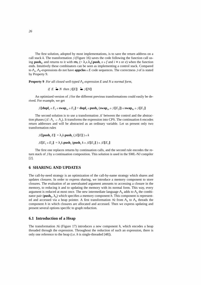
26

The first solution, adopted by most implementations, is to save the return address on acall stackk. The transformationS (Figure 16) saves the code following the function call us-ing pushk, and returns to it withrts i (= λix.λkf.pushi x o f and i ≡ s or e) when the functionends. Intuitively these combinators can be seen as implementing a control stack. Comparedto Λe, Λk-expressions do not haveappcloso E code sequences. The correctnessS of is statedby Property 9.

Property 9 For all closed well-typedΛe-expression E and N a normal form,

if E * N thenS [[E]] *

S [[N]]

An optimized version ofS for the different previous transformations could easily be de-rived. For example, we get

S [[duple o E1 o swapseo E2]] = duple o pushk (swapseo S [[E2]]) o swapke o S [[E1]]

The second solution is to use a transformationSl between the control and the abstrac-tion phases (Sl : Λs → Λs). It transforms the expression into CPS. The continuationk encodesreturn addresses and will be abstracted as an ordinary variable. Let us present only twotransformation rules

Sl [[pushs E]] = λsk.pushs (Sl [[E]] ) o k

Sl [[E1 o E2]] = λsk.pushs (pushs k o Sl [[E2]] ) o Sl [[E1]]

The first one replaces returns by continuation calls, and the second rule encodes the re-turn stack ofS by a continuation composition. This solution is used in the SML-NJ compiler[2].

6 SHARING AND UPDATES

The call-by-need strategy is an optimization of the call-by-name strategy which shares andupdates closures. In order to express sharing, we introduce a memory component to storeclosures. The evaluation of an unevaluated argument amounts to accessing a closure in thememory, to reducing it and to updating the memory with its normal form. This way, everyargument is reduced at most once. The new intermediate languageΛh adds toΛk the combi-nator pair (pushh, λh) which specifies a memory componenth. This component is represent-ed and accessed via a heap pointer. A first transformationHc from Λk to Λh threads thecomponenth in which closures are allocated and accessed. Then we express updating andpresent several options specific to graph reduction.

6.1 Introduction of a Heap

The transformationHc (Figure 17) introduces a new componenth, which encodes a heapthreaded through the expression. Throughout the reduction of such an expression, there isonly one reference to the heap (i.e.h is single-threaded [48]).

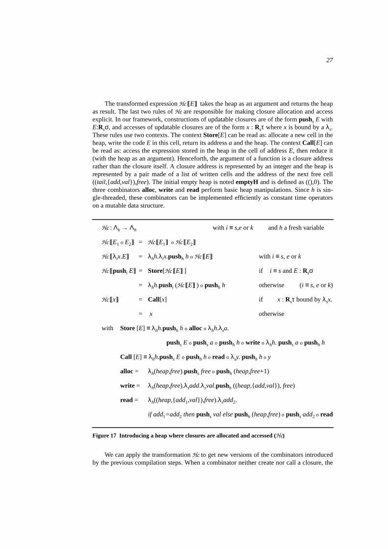
27

The transformed expressionHc [[E]] takes the heap as an argument and returns the heapas result. The last two rules ofHc are responsible for making closure allocation and accessexplicit. In our framework, constructions of updatable closures are of the formpushs E withE:Rsσ, and accesses of updatable closures are of the formx : Rsτ wherex is bound by aλs.These rules use two contexts. The contextStore[E] can be read as: allocate a new cell in theheap, write the codeE in this cell, return its addressa and the heap. The contextCall[E] canbe read as: access the expression stored in the heap in the cell of addressE, then reduce it(with the heap as an argument). Henceforth, the argument of a function is a closure addressrather than the closure itself. A closure address is represented by an integer and the heap isrepresented by a pair made of a list of written cells and the address of the next free cell((tail,add,val), free). The initial empty heap is notedemptyH and is defined as ((),0). Thethree combinatorsalloc, write andread perform basic heap manipulations. Sinceh is sin-gle-threaded, these combinators can be implemented efficiently as constant time operatorson a mutable data structure.

Hc : Λk → Λh with i ≡ s,e or k andh a fresh variable

Hc [[E1 o E2]] = Hc [[E1]] o Hc [[E2]]

Hc [[λix.E]] = λhh.λix.pushh h o Hc [[E]] with i ≡ s, e or k

Hc [[pushi E]] = Store[Hc [[E]] ] if i ≡ s andE : Rsσ

= λhh.pushi (Hc [[E]] ) o pushh h otherwise (i ≡ s, e or k)

Hc [[x]] = Call[x] if x : Rsτ bound byλsx.

= x otherwise

with Store [E] ≡ λhh.pushh h o alloc o λhh.λsa.

pushs E o pushs a o pushh h o write o λhh. pushs a o pushh h

Call [E] ≡ λhh.pushs E o pushh h o read o λsy. pushh h o y

alloc = λh(heap,free).pushs free o pushh (heap,free+1)

write = λh(heap,free).λsadd.λsval.pushh ((heap,add,val), free)

read = λh((heap,add1,val) ,free).λsadd2.

if add1=add2 thenpushs val elsepushh (heap,free) o pushs add2 o read

Figure 17 Introducing a heap where closures are allocated and accessed (Hc)

We can apply the transformationHc to get new versions of the combinators introducedby the previous compilation steps. When a combinator neither create nor call a closure, the

28

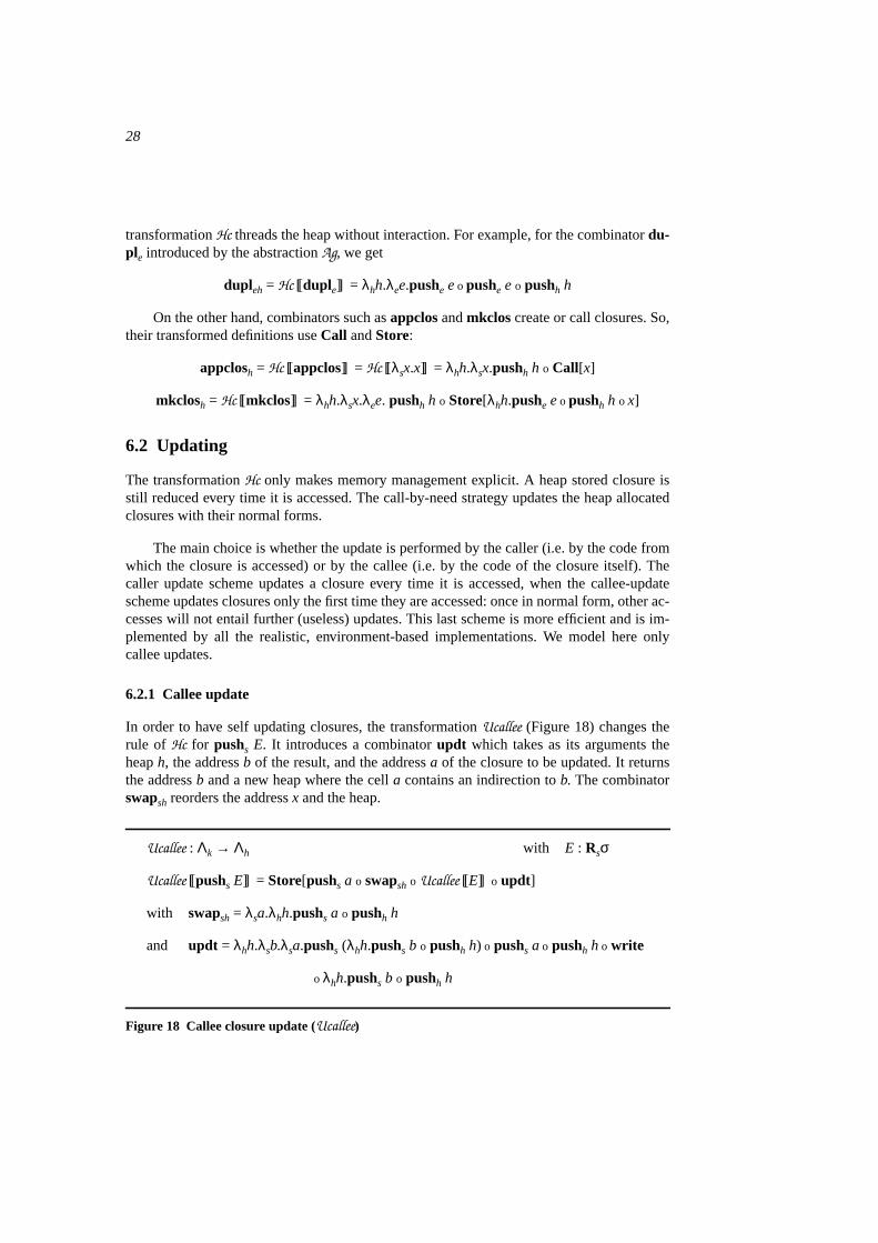
transformationHc threads the heap without interaction. For example, for the combinatordu-ple introduced by the abstractionAg, we get

dupleh = Hc [[duple]] = λhh.λee.pushe e o pushe e o pushh h

On the other hand, combinators such asappclos andmkclos create or call closures. So,their transformed definitions useCall andStore:

appclosh = Hc [[appclos]] = Hc [[λsx.x]] = λhh.λsx.pushh h o Call[x]

mkclosh = Hc [[mkclos]] = λhh.λsx.λee. pushh h o Store[λhh.pushe e o pushh h o x]

6.2 Updating

The transformationHc only makes memory management explicit. A heap stored closure isstill reduced every time it is accessed. The call-by-need strategy updates the heap allocatedclosures with their normal forms.

The main choice is whether the update is performed by the caller (i.e. by the code fromwhich the closure is accessed) or by the callee (i.e. by the code of the closure itself). Thecaller update scheme updates a closure every time it is accessed, when the callee-updatescheme updates closures only the first time they are accessed: once in normal form, other ac-cesses will not entail further (useless) updates. This last scheme is more efficient and is im-plemented by all the realistic, environment-based implementations. We model here onlycallee updates.

6.2.1 Callee update

In order to have self updating closures, the transformationUcallee (Figure 18) changes therule of Hc for pushs E. It introduces a combinatorupdt which takes as its arguments theheaph, the addressb of the result, and the addressa of the closure to be updated. It returnsthe addressb and a new heap where the cella contains an indirection tob. The combinatorswapsh reorders the addressx and the heap.

Ucallee : Λk → Λh with E : Rsσ

Ucallee [[pushs E]] = Store[pushs a o swapsh o Ucallee [[E]] o updt]

with swapsh = λsa.λhh.pushs a o pushh h

and updt = λhh.λsb.λsa.pushs (λhh.pushs b o pushh h) o pushs a o pushh h o write

o λhh.pushs b o pushh h

Figure 18 Callee closure update (Ucallee)

29

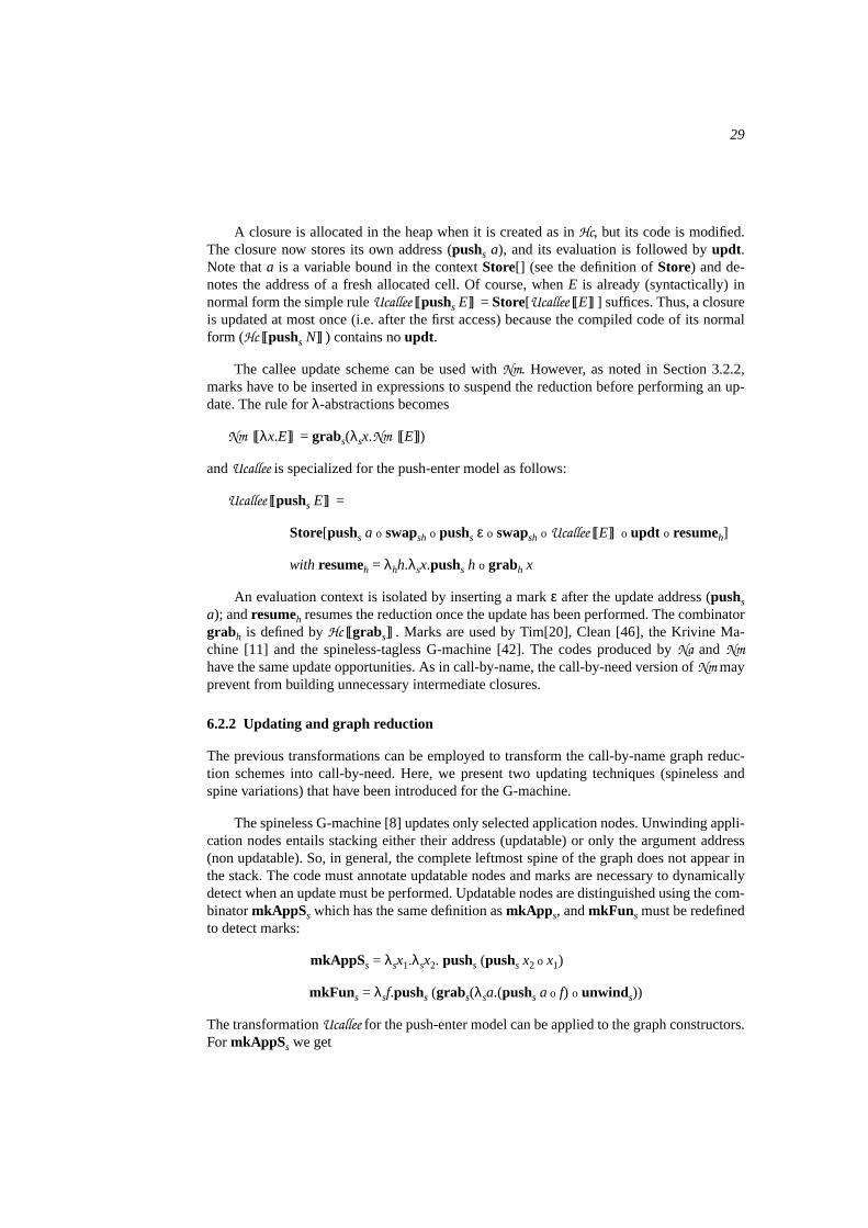
A closure is allocated in the heap when it is created as inHc, but its code is modified.The closure now stores its own address (pushs a), and its evaluation is followed byupdt.Note thata is a variable bound in the contextStore[] (see the definition ofStore) and de-notes the address of a fresh allocated cell. Of course, whenE is already (syntactically) innormal form the simple ruleUcallee [[pushs E]] = Store[Ucallee [[E]] ] suffices. Thus, a closureis updated at most once (i.e. after the first access) because the compiled code of its normalform (Hc [[pushs N]] ) contains noupdt.

The callee update scheme can be used withNm. However, as noted in Section 3.2.2,marks have to be inserted in expressions to suspend the reduction before performing an up-date. The rule forλ-abstractions becomes

Nm [[λx.E]] = grabs(λsx.Nm [[E]])

andUcallee is specialized for the push-enter model as follows:

Ucallee [[pushs E]] =

Store[pushs a o swapsh o pushs ε o swapsh o Ucallee [[E]] o updt o resumeh]

with resumeh = λhh.λsx.pushs h o grabh x

An evaluation context is isolated by inserting a markε after the update address (pushsa); andresumeh resumes the reduction once the update has been performed. The combinatorgrabh is defined byHc [[grabs]] . Marks are used by Tim[20], Clean [46], the Krivine Ma-chine [11] and the spineless-tagless G-machine [42]. The codes produced byNa and Nmhave the same update opportunities. As in call-by-name, the call-by-need version ofNm mayprevent from building unnecessary intermediate closures.

6.2.2 Updating and graph reduction

The previous transformations can be employed to transform the call-by-name graph reduc-tion schemes into call-by-need. Here, we present two updating techniques (spineless andspine variations) that have been introduced for the G-machine.

The spineless G-machine [8] updates only selected application nodes. Unwinding appli-cation nodes entails stacking either their address (updatable) or only the argument address(non updatable). So, in general, the complete leftmost spine of the graph does not appear inthe stack. The code must annotate updatable nodes and marks are necessary to dynamicallydetect when an update must be performed. Updatable nodes are distinguished using the com-binatormkAppSs which has the same definition asmkApp s, andmkFuns must be redefinedto detect marks:

mkAppSs = λsx1.λsx2. pushs (pushs x2 o x1)

mkFuns = λsf.pushs (grabs(λsa.(pushs a o f) o unwinds))

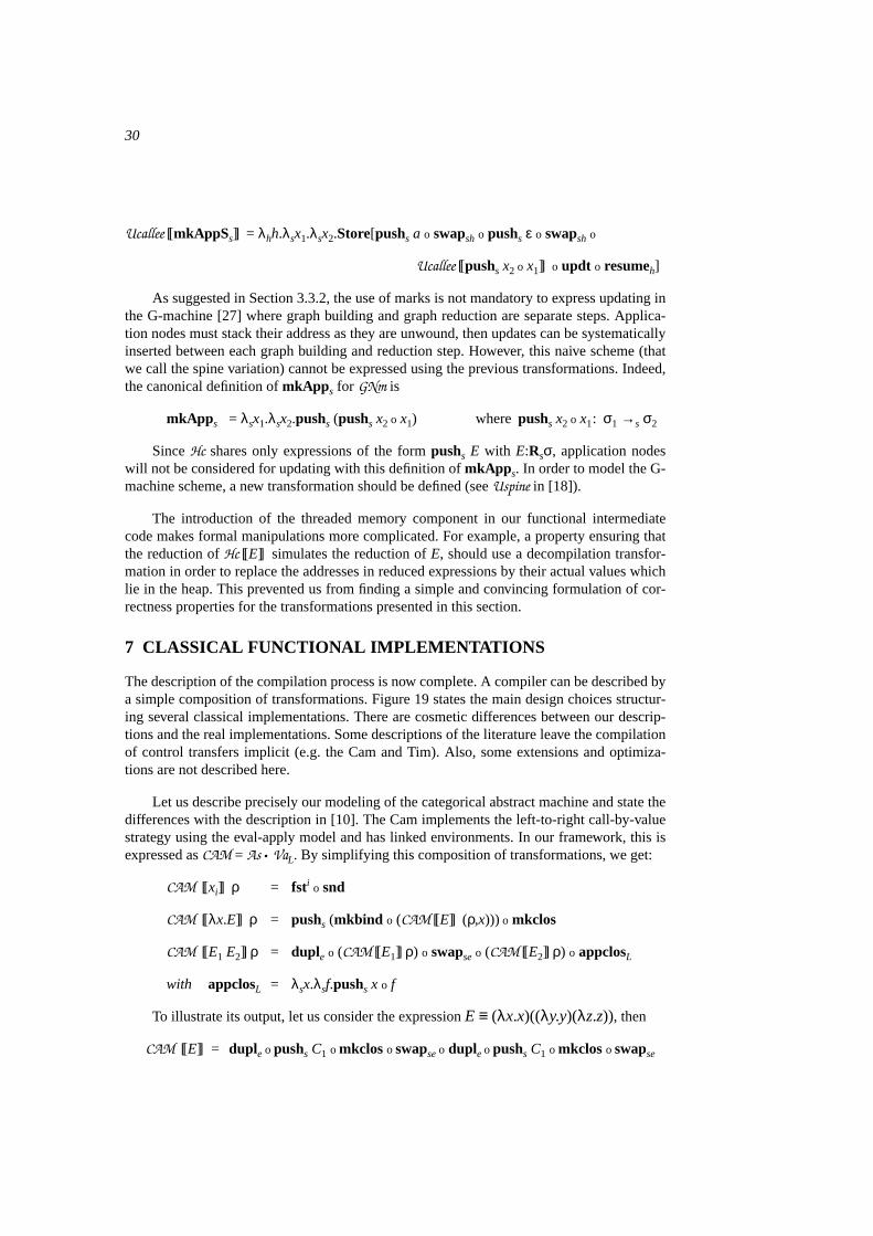
The transformationUcallee for the push-enter model can be applied to the graph constructors.For mkAppSs we get

30

Ucallee [[mkAppSs]] = λhh.λsx1.λsx2.Store[pushs a o swapsh o pushs ε o swapsh o

Ucallee [[pushs x2 o x1]] o updt o resumeh]

As suggested in Section 3.3.2, the use of marks is not mandatory to express updating inthe G-machine [27] where graph building and graph reduction are separate steps. Applica-tion nodes must stack their address as they are unwound, then updates can be systematicallyinserted between each graph building and reduction step. However, this naive scheme (thatwe call the spine variation) cannot be expressed using the previous transformations. Indeed,the canonical definition ofmkApp s for GNm is

mkApp s = λsx1.λsx2.pushs (pushs x2 o x1) where pushs x2 o x1 : σ1 →s σ2

SinceHc shares only expressions of the formpushs E with E:Rsσ, application nodeswill not be considered for updating with this definition ofmkApp s. In order to model the G-machine scheme, a new transformation should be defined (seeUspine in [18]).

The introduction of the threaded memory component in our functional intermediatecode makes formal manipulations more complicated. For example, a property ensuring thatthe reduction ofHc [[E]] simulates the reduction ofE, should use a decompilation transfor-mation in order to replace the addresses in reduced expressions by their actual values whichlie in the heap. This prevented us from finding a simple and convincing formulation of cor-rectness properties for the transformations presented in this section.

7 CLASSICAL FUNCTIONAL IMPLEMENTATIONS

The description of the compilation process is now complete. A compiler can be described bya simple composition of transformations. Figure 19 states the main design choices structur-ing several classical implementations. There are cosmetic differences between our descrip-tions and the real implementations. Some descriptions of the literature leave the compilationof control transfers implicit (e.g. the Cam and Tim). Also, some extensions and optimiza-tions are not described here.

Let us describe precisely our modeling of the categorical abstract machine and state thedifferences with the description in [10]. The Cam implements the left-to-right call-by-valuestrategy using the eval-apply model and has linked environments. In our framework, this isexpressed asCAM = As • VaL. By simplifying this composition of transformations, we get:

CAM [[xi]] ρ = fsti o snd

CAM [[λx.E]] ρ = pushs (mkbind o (CAM [[E]] (ρ,x))) o mkclos

CAM [[E1 E2]] ρ = duple o (CAM [[E1]] ρ) o swapseo (CAM [[E2]] ρ) o appclosL

with appclosL = λsx.λsf.pushs x o f

To illustrate its output, let us consider the expressionE ≡ (λx.x)((λy.y)(λz.z)), then

CAM [[E]] = duple o pushs C1 o mkclos o swapse o dupleo pushs C1 o mkclos o swapse

31

o pushs C1 o mkclos o appclosL o appclosL

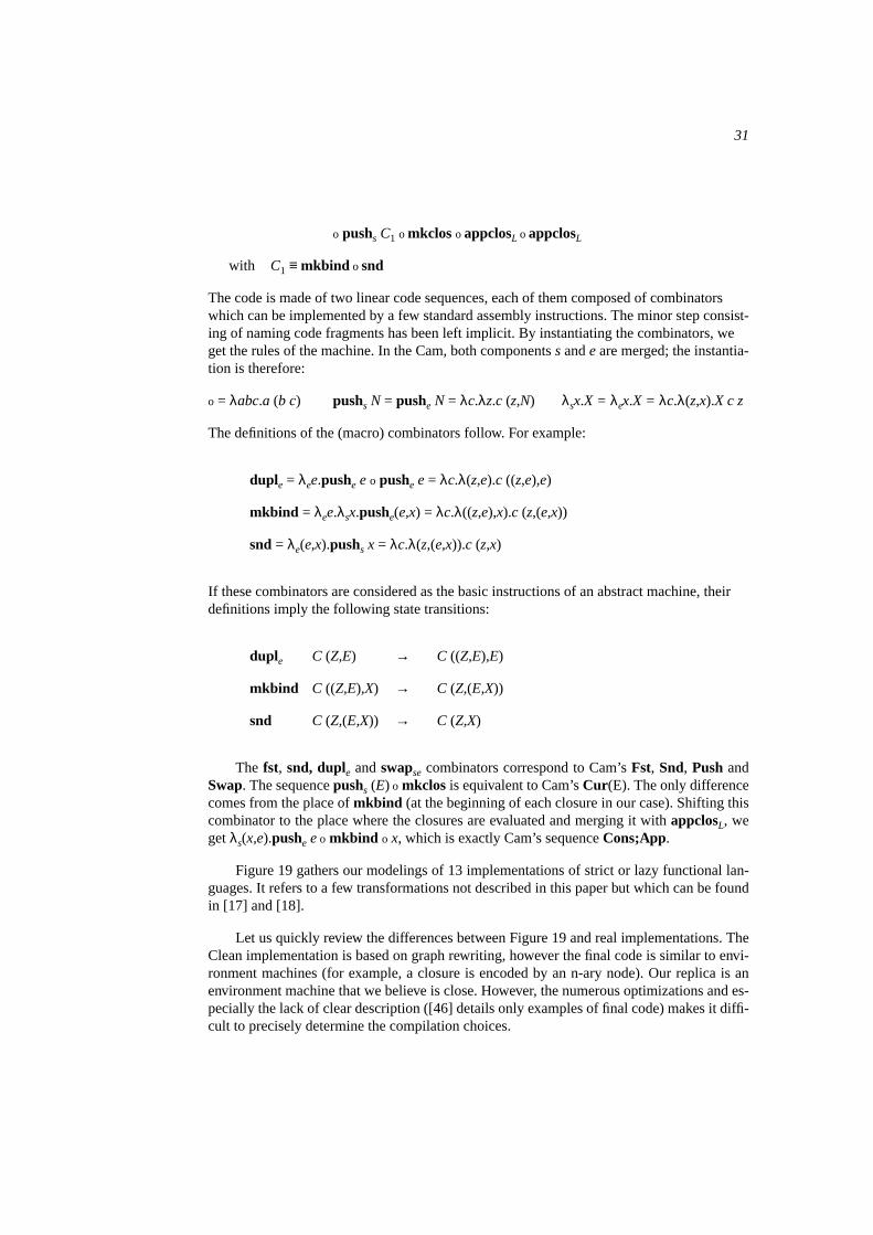
with C1 ≡ mkbind o snd

The code is made of two linear code sequences, each of them composed of combinatorswhich can be implemented by a few standard assembly instructions. The minor step consist-ing of naming code fragments has been left implicit. By instantiating the combinators, weget the rules of the machine. In the Cam, both componentss ande are merged; the instantia-tion is therefore:

o = λabc.a (b c) pushs N = pushe N = λc.λz.c (z,N) λsx.X = λex.X = λc.λ(z,x).X c z

The definitions of the (macro) combinators follow. For example:

duple = λee.pushe e o pushe e= λc.λ(z,e).c ((z,e),e)

mkbind = λee.λsx.pushe(e,x) = λc.λ((z,e),x).c (z,(e,x))

snd = λe(e,x).pushs x = λc.λ(z,(e,x)).c (z,x)

If these combinators are considered as the basic instructions of an abstract machine, theirdefinitions imply the following state transitions:

duple C (Z,E) → C ((Z,E),E)

mkbind C ((Z,E),X) → C (Z,(E,X))

snd C (Z,(E,X)) → C (Z,X)

The fst, snd, duple andswapse combinators correspond to Cam’sFst, Snd, Push andSwap. The sequencepushs (E) o mkclos is equivalent to Cam’sCur (E). The only differencecomes from the place ofmkbind (at the beginning of each closure in our case). Shifting thiscombinator to the place where the closures are evaluated and merging it withappclosL, wegetλs(x,e).pushe e o mkbind o x, which is exactly Cam’s sequenceCons;App.

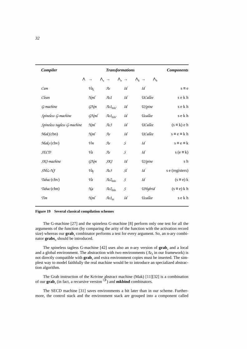
Figure 19 gathers our modelings of 13 implementations of strict or lazy functional lan-guages. It refers to a few transformations not described in this paper but which can be foundin [17] and [18].

Let us quickly review the differences between Figure 19 and real implementations. TheClean implementation is based on graph rewriting, however the final code is similar to envi-ronment machines (for example, a closure is encoded by an n-ary node). Our replica is anenvironment machine that we believe is close. However, the numerous optimizations and es-pecially the lack of clear description ([46] details only examples of final code) makes it diffi-cult to precisely determine the compilation choices.

32

Compiler Transformations Components

Λ → Λs → Λe → Λk → Λh

Cam VaL As Id Id s≡ e

Clean Nml Ac1 Id UCallee s e k h

G-machine GNm Ac1dsb’ Id USpine s e k h

Spineless G-machine GNml Ac1dsb’ Id Ucallee s e k h

Spineless tagless G-machine Nml Ac3 Id UCallee (s≡ k) e h

Mak (cbn) Nml As Id UCallee s≡ e ≡ k h

Maks (cbv) Vm As S Id s≡ e ≡ k

SECD Va As S Id s (e≡ k)

SKI-machine GNm SKI Id USpine s h

SML-NJ Vaf Ac3 Sl Id s e (registers)

Tabac (cbv) Va Ac2dsb S Id (s≡ e) k

Tabac (cbn) Na Ac2dsb S UHybrid (s≡ e) k h

Tim Nml Ac1m Id Ucallee s e k h

Figure 19 Several classical compilation schemes

The G-machine [27] and the spineless G-machine [8] perform only one test for all thearguments of the function (by comparing the arity of the function with the activation recordsize) whereas ourgrabs combinator performs a test for every argument. So, an n-ary combi-natorgrabsn should be introduced.

The spineless tagless G-machine [42] uses also an n-ary version ofgrabs and a localand a global environment. The abstraction with two environments (Ac3 in our framework) isnot directly compatible withgrabs and extra environment copies must be inserted. The sim-plest way to model faithfully the real machine would be to introduce an specialized abstrac-tion algorithm.

The Grab instruction of the Krivine abstract machine (Mak) [11][32] is a combinationof ourgrabs (in fact, a recursive version

i) andmkbind combinators.

The SECD machine [31] saves environments a bit later than in our scheme. Further-more, the control stack and the environment stack are grouped into a component called

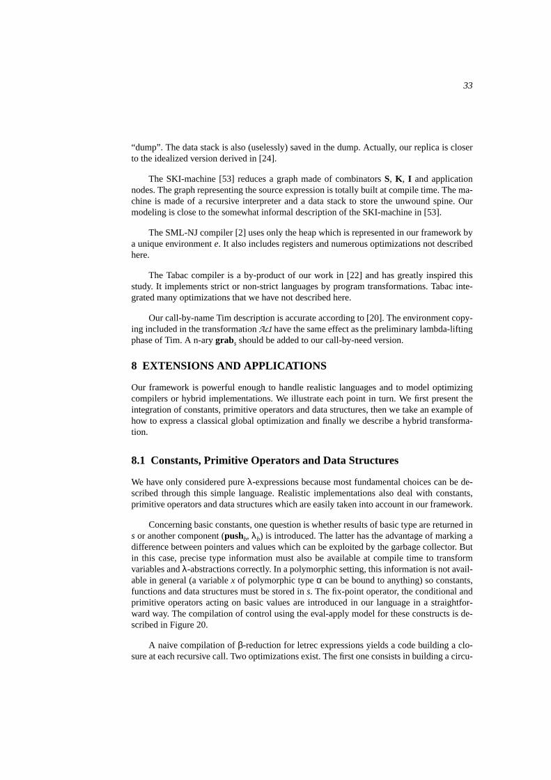
33

“dump”. The data stack is also (uselessly) saved in the dump. Actually, our replica is closerto the idealized version derived in [24].

The SKI-machine [53] reduces a graph made of combinatorsS, K , I and applicationnodes. The graph representing the source expression is totally built at compile time. The ma-chine is made of a recursive interpreter and a data stack to store the unwound spine. Ourmodeling is close to the somewhat informal description of the SKI-machine in [53].

The SML-NJ compiler [2] uses only the heap which is represented in our framework bya unique environmente. It also includes registers and numerous optimizations not describedhere.

The Tabac compiler is a by-product of our work in [22] and has greatly inspired thisstudy. It implements strict or non-strict languages by program transformations. Tabac inte-grated many optimizations that we have not described here.

Our call-by-name Tim description is accurate according to [20]. The environment copy-ing included in the transformationAc1 have the same effect as the preliminary lambda-liftingphase of Tim. A n-arygrabs should be added to our call-by-need version.

8 EXTENSIONS AND APPLICATIONS

Our framework is powerful enough to handle realistic languages and to model optimizingcompilers or hybrid implementations. We illustrate each point in turn. We first present theintegration of constants, primitive operators and data structures, then we take an example ofhow to express a classical global optimization and finally we describe a hybrid transforma-tion.

8.1 Constants, Primitive Operators and Data Structures

We have only considered pureλ-expressions because most fundamental choices can be de-scribed through this simple language. Realistic implementations also deal with constants,primitive operators and data structures which are easily taken into account in our framework.

Concerning basic constants, one question is whether results of basic type are returned ins or another component (pushb, λb) is introduced. The latter has the advantage of marking adifference between pointers and values which can be exploited by the garbage collector. Butin this case, precise type information must also be available at compile time to transformvariables andλ-abstractions correctly. In a polymorphic setting, this information is not avail-able in general (a variablex of polymorphic typeα can be bound to anything) so constants,functions and data structures must be stored ins. The fix-point operator, the conditional andprimitive operators acting on basic values are introduced in our language in a straightfor-ward way. The compilation of control using the eval-apply model for these constructs is de-scribed in Figure 20.

A naive compilation ofβ-reduction for letrec expressions yields a code building a clo-sure at each recursive call. Two optimizations exist. The first one consists in building a circu-

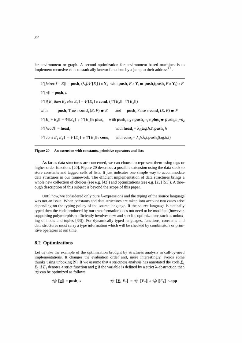
34

lar environment or graph. A second optimization for environment based machines is toimplement recursive calls to statically known functions by a jump to their addressp .

V [[ letrec f= E]] = pushs (λsf.V [[E]] ) o Ys with pushs F o Ys pushs(pushs F o Ys) o F

V [[n]] = pushs n

V [[ if E1 then E2 else E3]] = V [[E1]] o conds (V [[E2]] , V [[E3]] )

with pushs Trueo conds (E, F) E and pushs Falseo conds (E, F) F

V [[E1 + E2]] = V [[E2]] o V [[E1]] o pluss with pushs n2 o pushsn1 o pluss pushsn1+n2

V [[head]] = heads with heads= λs(tag,h,t).pushs h

V [[cons E1 E2]] = V [[E2]] o V [[E1]] o conss with conss= λsh.λst.pushs(tag,h,t)

Figure 20 An extension with constants, primitive operators and lists

As far as data structures are concerned, we can choose to represent them using tags orhigher-order functions [20]. Figure 20 describes a possible extension using the data stack tostore constants and tagged cells of lists. It just indicates one simple way to accommodatedata structures in our framework. The efficient implementation of data structures brings awhole new collection of choices (see e.g. [42]) and optimizations (see e.g. [23] [51]). A thor-ough description of this subject is beyond the scope of this paper.

Until now, we considered only pureλ-expressions and the typing of the source languagewas not an issue. When constants and data structures are taken into account two cases arisedepending on the typing policy of the source language. If the source language is staticallytyped then the code produced by our transformation does not need to be modified (however,supporting polymorphism efficiently involves new and specific optimizations such as unbox-ing of floats and tuples [33]). For dynamically typed languages, functions, constants anddata structures must carry a type information which will be checked by combinators or prim-itive operators at run time.

8.2 Optimizations

Let us take the example of the optimization brought by strictness analysis in call-by-needimplementations. It changes the evaluation order and, more interestingly, avoids somethunks using unboxing [9]. If we assume that a strictness analysis has annotated the codeE1E2 if E1 denotes a strict function andx if the variable is defined by a strictλ-abstraction thenNa can be optimized as follows

Na [[x]] = pushs x Na [[E1 E2]] = Na [[E2]] o Na [[E1]] o app

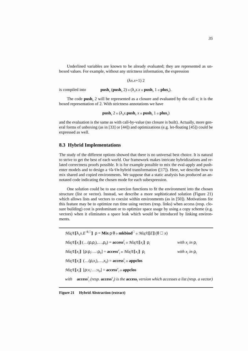
35

Underlined variables are known to be already evaluated; they are represented as un-boxed values. For example, without any strictness information, the expression

(λx.x+1) 2

is compiled into pushs (pushs 2) o (λsx.x o pushs 1 o pluss).

The codepushs 2 will be represented as a closure and evaluated by the callx; it is theboxed representation of 2. With strictness annotations we have

pushs 2 o (λsx.pushs x o pushs 1 o pluss)

and the evaluation is the same as with call-by-value (no closure is built). Actually, more gen-eral forms of unboxing (as in [33] or [44]) and optimizations (e.g. let-floating [45]) could beexpressed as well.

8.3 Hybrid Implementations

The study of the different options showed that there is no universal best choice. It is naturalto strive to get the best of each world. Our framework makes intricate hybridizations and re-lated correctness proofs possible. It is for example possible to mix the eval-apply and push-enter models and to design aVa-Vm hybrid transformation ([17]). Here, we describe how tomix shared and copied environments. We suppose that a static analysis has produced an an-notated code indicating the chosen mode for each subexpression.

One solution could be to use coercion functions to fit the environment into the chosenstructure (list or vector). Instead, we describe a more sophisticated solution (Figure 21)which allows lists and vectors to coexist within environments (as in [50]). Motivations forthis feature may be to optimize run time using vectors (resp. links) when access (resp. clo-sure building) cost is predominant or to optimize space usage by using a copy scheme (e.g.vectors) when it eliminates a space leak which would be introduced by linking environ-ments.

MixA [[λsx.E θ,⊕]] ρ = Mix ρ θ o mkbind⊕ o MixA [[E]] (θ ⊕ x)

MixA [[xi]] (…(ρ,ρi),…,ρ0) = accessli o MixA [[xi]] ρi with xi in ρi

MixA [[xi]] [ ρ:ρi:…:ρ0] = accessvi o MixA [[xi]] ρi with xi in ρi

MixA [[xi]] (…(ρ,xi),…,x0) = accessli o appclos

MixA [[xi]] [ ρ:xi:…:x0] = accessvi o appclos

with accessli (resp.accessvi) is theaccessi version which accesses a list (resp. a vector)

Figure 21 Hybrid Abstraction (extract)

36

Eachλ-abstraction is annotated by a new mixed environment structureθ and ⊕ (∈v,l) which indicates how to bind the current value (as a vector “v” or as a link “l”). Mixedstructures are built bymkbind v, mkbind l and the macro-combinatorMix which copies andrestructures the environmentρ according to the annotationθ (Figure 21). Paths to values arenow expressed by sequences ofaccessli andaccessvi. The abstraction algorithm distinguishesvectors from lists in the compile time environment using constructors “:” and “,”.

9 RELATED WORK

We review in this section the different formalisms used in the description of functional im-plementations: theλ-calculus,λ-calculi with explicit substitutions, combinators, monads.We also present papers comparing specific implementations and the related area of seman-tic-directed compiler derivation.

Our approach and this paper stem from our previous work on compilation of functionallanguages by program transformation [22]. Our goal then was to show that the whole imple-mentation process could be described in the functional framework. The two main steps werethe compilation of control using a CPS conversion and the compilation of theβ-reductionusing indexed combinators that could be seen as basic instructions on a stack. We remainedthroughout within theλ-calculus and did not have to introduce an ad-hoc abstract machine.We described only one particular implementation; our main motivation was to make correct-ness proofs of realistic implementations simpler not to describe and compare various imple-mentation techniques. The SML-NJ compiler has also been described using programtransformations including CPS and closure conversions [2]. Other compilers use the CPStransformation to encode the reduction strategy within theλ-calculus [30][52]. Encodingimplementation issues within theλ-calculus leads to complex expressions (e.g. sequencingis coded as a composition of continuations). The constructorspushi, o and λi make ourframework more abstract and simplify the expressions. The instantiation of these construc-tors asλ-expressions provides an interesting new implementation step (Section 2.5): thechoice of the number and the representation of the components of the underlying abstractmachine are kept apart. Within theλ-calculus, one has to choose before describing an imple-mentation whether, for example, data and environments are stored in two separate compo-nents or in a single one.

The de Bruijnλ-calculus [14], which uses indices instead of variables, has been used asan intermediate language by several abstract machines. As we saw in Section 4.1.2, a deBruijn index can be seen as the address of a value in the run-time environment. A collectionof formalisms, theλ-calculi with explicit substitutions, emphasize also the environmentmanagement and can be seen as calculi of closures [1]. These calculi help formal reasoningon substitution and make some implementation details explicit. However, important imple-mentation choices such as the representation of the environments (lists or vectors) are, ingeneral, not tackled in these formalisms. Hardin &al. [25] introduceλσw, a weakλ-calculuswith explicit substitutions, which can serve as the output language of functional compilers.They describe several abstract machines in this framework. However, their goal is to exhibitthe common points of implementations not to model precisely existing implementations.Another variant,λσw

a [7], can describe sharing and eases the proofs concerning memory

37

management. Theλσwa -expressions stay at a higher level than real machine code since, for

example, sharing is modeled by formal labels and parallel reductions.

A closely related framework used as intermediate language is combinatory logic [13].Combinators have been used to encode the compilation of theβ-reduction. Some compila-tion issues, such as the representation of environments, are usually not dealt with. Differentset of combinators, such as S,K ,I ,B,C[53], have been used to define abstraction algo-rithms for graph reducers [28][36]. The categorical combinators [12] have been used in envi-ronment machines such as the Cam [10] and the Krivine machine [4].

Arising from different roots, our first intermediate languageΛs is surprisingly close toMoggi’s computational metalanguage [40]. In particular, we may interpret the monadic con-struct [E] aspushs E and (let x ⇐ E1 in E2) asE1 o λsx.E2 and get back the monadic laws(let.β), (let.η) and (ass). The monadic framework is more abstract. For example, one canwrite monadic expressions such as

let _ ⇐ writeStack(X) in (let e ⇐ readEnv()in E)

whereas, in our formalism, we need to reorder data and environment with aswap combina-tor:

pushs X o swapseo λee.E

These administrative combinators allow us to merge several components in the instanti-ation step. The abstract features of monads can be an hindrance to express low level imple-mentation details and to get closer to a machine code. For example, the monadic call-by-value CPS expression (let a ⇐ A in (let f ⇐ F in [ f a])) evaluates the argumentA, the func-tion F and returns the application (f a), but does not state if the application is reduced beforeit is returned. InΛs, we disallow unrestricted applications and make the previous reductionexplicit with anapp combinator. A key feature of our approach is to describe and structurethe compilation process as a composition of individualized transformations. The monadicframework does not appear to be well suited to this purpose since monads are notoriouslydifficult to compose. Liang & al. [35] needs complex parametrized monads to describe andcompose different compilation steps. The difficulties to compose monads and to representlow level details are serious drawbacks with respect to our goals. Overall, the monadicframework is a general tool to structure functional programs [55] whereas our small frame-work has been tailor-made to describe implementations.

Besides benchmarks, few functional language implementations have been compared.Some particular compilation steps have been studied. For example, [28] compare differentabstraction algorithms and [26] expresses CPS transformations in the monadic framework.A few works explore the relationship between two abstract machines such as CMC and Tim[37] and Tim and the G-machine [43]. Their goal is to show the equivalence between seem-ingly very different implementations. CMC and Tim are compared by defining transforma-tions between the states of the two machines. The comparison of Tim and the G-machine ismore informal but highlights the relationship between an environment machine and a graphreducer. Also, let us mention Asperti [4] who provides a categorical understanding of theKrivine machine and an extended Cam and Crégut [11] who has studied the relationship be-

38

tween the Tim and the Krivine machine. All these implementation comparisons focus onparticular compilation steps or machines but do not define a global approach to compare im-plementations.

Related work also includes the derivation of abstract machines from denotational or op-erational semantics. Starting from a denotational semantics with continuations, Wand [56]compiles theβ-reduction using combinators and linearizes expressions in sequences of ab-stract code. The semantics of the program is translated into a sequence representing the codeand a machine to execute it. In our approach, semantics or machines do not appear explicitly.Hannan [24] and Sestoft [49] start from a “big step” (natural) operational semantics, incre-mentally suppress ambiguities (e.g. impose a left-to-right reduction order) and refine com-plex operation (e.g.β-reduction), until they get a “small step” (structural) operationalsemantics. Some of the refinement steps have to deal with operations specific to their frame-work (e.g. suppressing unification). Meijer [38] uses program algebra to calculate some sim-ple compilers from a denotational semantics via a series of refinements. All these derivationtechniques aim at providing a methodology to formally develop implementations from se-mantics. Their focus is on the refinement process and correction issues and, usually, they de-scribe the derivation of a single implementation. Not surprisingly, the derived compilers donot model precisely existing implementations. They are best described as idealized than so-phisticated or optimized implementations. Comparisons of implementation choices seemharder with a description based on semantics refinement than with a description by programtransformations. Also, some choices seem difficult to naturally obtain by derivation (e.g. thepush-enter model for call-by-value). On the other hand, these semantics based methodolo-gies can potentially be applied to any language that can be described in their semanticsframework.

10 CONCLUSION

Let us review the implementation choices encountered in our study. The most significantchoice for the compilation of control is using the eval-apply model (Va, Na) or the push-en-ter model (Vm, Nm). There are other minor options such as stackless variations (Vaf, Naf) orright-to-leftvs. left-to-right call-by-value. We have shown that the transformations employedby graph reducers can be seen as interpretative versions of the environment-based transfor-mations. For the compilation ofβ-reduction, the main choice is using environment-less (e.g.SKI) abstraction algorithms, list-like (shared) environments (As) or vector-like (copied) en-vironments (Ac). For the latter choice, there are several transformations depending on theway environments are copied (Ac1, Ac2, Ac3). Actually, a complete family of generic trans-formations modeling different managements of the environment stack can be derived. Forcontrol transfers, one can introduce a return address stack or use CPS conversion. Self up-datable closures (i.e. callee update) is the standard way to implement updating but graph re-duction brings other options.

Our approach focuses on (but is not restricted to) the description and comparison offundamental options. The transformations are designed to model a precise compilation step;they are generic with respect to the other steps. It is then not surprising that, often, simplecompositions of transformations do not model accurately real implementations whose de-

39

sign is more ad-hoc than generic. In most cases, the differences are nevertheless superficialand it is sufficient to specialize the transformations to obtain existing implementations.

The use of program transformations appears to be well suited to precisely and com-pletely model the compilation process. Many standard optimizations (uncurrying, unboxing,hoisting, peephole optimizations) can be expressed as program transformations as well. Thisunified framework simplifies correctness proofs. For example, we do not introduce explicitlyan abstract machine and therefore we do not have to prove that its operational definition iscoherent with the semantics of the language (as in [47] and [34]). Program transformationsmakes it possible to reason about the efficiency of the produced code as well as about thecomplexity of transformations themselves. Actually, these advantages appear clearly beforethe last compilation step. The introduction of a threaded state seriously complicates programmanipulations and correctness proofs. This is not surprising because our final code is similarto a real assembly code.

Our main goal was to structure and clarify the design space of functional language im-plementations. The exploration is still far from complete. There are still many avenues forfurther research:

• It would be interesting to give a concrete form to our framework by implementing all thetransformations presented. This compiler construction workbench would make it possi-ble to implement a wide variety of implementations just by composing transformations.This would be useful to try completely new associations of compilation choices and toassess the implementations and optimizations in practice.

• A last step towards high quality machine code would be the modeling of register alloca-tion. This could be done via the introduction of another component: a vector of registers.

• A systematic description of standard optimizations and program transformations shouldbe undertaken. A benefit would be to clarify the impact of a program transformation de-pending on the implementation choices. Let us consider, for example,λ-lifting, a contro-versial transformation [27][39]. Intuitively, λ-lifting can be beneficial forimplementations using linked environments. Indeed, in this case, its effect is to shortenaccesses to variables by performing copies. Whether the gain is worth the cost dependson how many times a variable is accessed. We believe that this question could be studiedand settled in our framework. Also, proving the correctness of optimizations based onstatic analyses is a difficult (and largely neglected) problem [9]. Expressing these optimi-zations as program transformations in our unified framework should make this task easi-er.

• Another research direction is the design of hybrid transformations (mixing several com-pilation schemes). We hinted at a solution to mix copied and linked environments in Sec-tion 8.3 and a solution to mix the eval-apply and the push-enter model in [18]. Othershybrid transformations as well as the analyses needed to make these transformationsworthwhile have yet to be devised. Without the help of a formal framework, such trans-formations would be quite difficult to design and prove correct. The description of previ-ously unknown compositions of transformations, the mechanical derivation of newabstraction algorithms and hybrid transformations all indicate that our approach can alsosuggest new implementation techniques.

40

• Many interesting formal comparisons of transformations remain to be done. At the mo-ment, we have just compared a few couples of transformations (Va andVm, Na andNm[18], As andAc1). It might be the case that a specific choice for a compilation step desig-nates a best candidate for the compilation of another step. This could be established bycomparing compositions of transformations (e.g.As • Va andAc1 • Va).

We believe that the accomplished work already shows that our framework is expressiveand powerful enough to tackle these problems.

AKNOWLEDGMENTS

We are grateful to Luke Hornof and Daniel Le Métayer for their comments on several ver-sions of this paper. Thanks are also due to the referees who provided helpful suggestions.

REFERENCES

[1] M. Abadi, L. Cardelli, P. L. Curien and J. J. Levy. Explicit Substitutions. In Proc ofPOPL’1990,pp. 31-46, 1990.

[2] A. W. Appel.Compiling with Continuations. Cambridge University Press. 1992.

[3] G. Argo. Improving the three instruction machine. InProc. of FPCA’89, pp. 100-115, 1989.

[4] A. Asperti. A categorical understanding of environment machines.Journal of Functional Pro-gramming, 2(1), pp. 23-59,1992.

[5] H.P. Barendregt.The lambda calculus. Its syntax and semantics. North-Holland, 1981.

[6] H.P. Barendregt and K. Hemerik. Types in lambda calculi and programming languages. In3rdEuropean Symp. on Programming, LNCS Vol. 432, pp. 1-35, 1990.

[7] Z. Benaissa, P. Lescanne and K. H. Rose: Modeling Sharing and Recursion for Weak ReductionStrategies Using Explicit Substitution. In Proc of PLILP’1996, pp. 393-407, 1996.

[8] G. Burn, S.L. Peyton Jones and J.D. Robson. The spineless G-machine. InProc. of LFP’88, pp.244-258, 1988.

[9] G. Burn and D. Le Métayer. Proving the correctness of compiler optimisations based on a globalanalysis.Journal of Functional Programming, 6(1), pp. 75-110, 1996.

[10] G. Cousineau, P.-L. Curien and M. Mauny, The categorical abstract machine.Science of Com-puter Programming, 8(2), pp. 173-202, 1987.

[11] P. Crégut.Machines à environnement pour la réduction symbolique et l’évaluation partielle.Thèse de l’université de Paris VII, 1991.

[12] P. L. Curien.Categorical Combinators, Sequential Algorithms and Functional Programming.Birkauser, 1993.

[13] H.B. Curry and R. Feys.Combinatory Logic, Vol. 1, North-Holland. 1958.

[14] N. G. De Brujin.λ-calculus notation with nameless dummies: a tool for automatic formula ma-nipulation, with application to Church Rosser theorem. InIndagationes mathematicae, 34, pp.381-392, 1972.

[15] O. Danvy. Back to direct style. InProc. of ESOP’92, LNCS Vol. 582, pp. 130-150, 1992.

[16] R. Douence and P. Fradet. Towards a taxonomy of functional language implementations. InProcof PLILP’95,LNCS 982, pp. 27-44, 1995.

41

[17] R. Douence and P. Fradet. A taxonomy of functional language implementations. Part I: call-by-value.INRIA research report 2783, Jan. 1996.

[18] R. Douence and P. Fradet. A taxonomy of functional language implementations. Part II: call-by-name, call-by-need, and graph reduction.INRIA research report 3050, Nov. 1996.

[19] R. Douence.Décrire et comparer les mises en œuvre de langages fonctionnels. PhD Thesis, Uni-versity of Rennes I, 1996.

[20] J. Fairbairn and S. Wray. Tim: a simple, lazy abstract machine to execute supercombinators. InProc of FPCA’87,LNCS 274, pp. 34-45, 1987.

[21] M. J. Fischer. Lambda-calculus schemata. InProc. of the ACM Conf. on Proving Propertiesabout Programs, Sigplan Notices, Vol. 7(1), pp. 104-109,1972.

[22] P. Fradet and D. Le Métayer. Compilation of functional languages by program transformation.ACM Trans. on Prog. Lang. and Sys., 13(1), pp. 21-51, 1991.

[23] C. Hall. Using Hindley-Milner type inference to optimise list representation. InProc. of LFP’94,pp. 162-172,1994.

[24] J. Hannan. From operational semantics to abstract machines.Math. Struct. in Comp. Sci.,2(4),pp. 415-459, 1992.

[25] T. Hardin, L. Maranget and B. Pagano. Functional back-ends within the lambda-sigma calculus.In Proc. ofICFP’1996, pp. 25-33, 1996.

[26] J. Hatcliff and O. Danvy. A generic account of continuation-passing styles. InProc. of POPL’94,pp. 458-471, 1994.

[27] T. Johnsson.Compiling Lazy Functional Languages. PhD Thesis, Chalmers University, 1987.

[28] M. S. Joy, V. J. Rayward-Smith and F. W. Burton. Efficient combinator code.Computer Lan-guages, 10(3), 1985.

[29] J.W. Klop. Term rewriting systems. InHandbook of Logic in Computer Science. Vol. 2, pp. 2-108, Oxford University Press, 1992.

[30] D. Kranz, R. Kesley, J. Rees, P. Hudak, J.Philbin, and N. Adams. ORBIT: An optimizing com-piler for Scheme.SIGPLAN Notices, 21(7), pp. 219-233, 1986.

[31] P. J. Landin. The mechanical evaluation of expressions.The Computer Journal, 6(4), pp. 308-320, 1964.

[32] X. Leroy. The Zinc experiment: an economical implementation of the ML language.INRIATechnical Report 117, 1990.

[33] X. Leroy. Unboxed objects and polymorphic typing. InACM Symp. on Princ. of Prog. Lang., pp.177-188, 1992.

[34] D. Lester,Combinator Graph Reduction: a congruence and its application. PhD thesis, OxfordUniversity, 1989.

[35] S. Liang, P. Hudak, M. P. Jones. Monad transformers and modular interpreters. In Proc. ofPOPL’95, pp. 333-343, 1995.

[36] R. D. Lins. Categorical multi-combinators. InProc. of FPCA’87, LNCS 274, pp. 60-79, 1987.

[37] R. Lins, S. Thompson and S.L. Peyton Jones. On the equivalence between CMC and TIM.Jour-nal of Functional Programming, 4(1), pp. 47-63, 1992.

[38] E. Meijer,Calculating Compilers. PhD thesis, Nijmegen University, 1992.

[39] E. Meijer and R. Paterson. Down with lambda lifting.Unpublished paper. copies available at:erik@cs.kun.nl, 1991.

[40] E. Moggi. Notions of computation and monads.Inf. and Comp., 93:55-92, 1991.

42

[41] S.L. Peyton-Jones.The implementation of functional programming languages.Prentice Hall,1987.

[42] S.L. Peyton Jones. Implementing lazy functional languages on stock hardware: the spinelesstagless G-machine.Journal of Func. Prog., 2(2):127-202, 1992.

[43] S. L. Peyton Jones and D. Lester.Implementing functional languages, a tutorial. Prentice Hall,1992.

[44] S. L. Peyton Jones and J. Launchbury. Unboxed values as first class citizens in a non-strict func-tional language. InProc. of FPCA’91, LNCS 523, pp. 636-666, 1991.

[45] S. L. Peyton Jones, W. Partain and A. Santos. Let-floating: moving bindings to give faster pro-grams. InProc. of ICFP’96, pp. 1-12, 1996.

[46] R. Plasmeijer and M. van Eekelen.Functional Programming and Parallel Graph Rewriting. Ad-dison-Wesley, 1993.

[47] G. D. Plotkin: Call-by-Name, Call-by-Value and the lambda-Calculus. InTCS 1(2), pp. 125-159,1975.

[48] D. Schmidt.Denotational Semantics, a Methodology for Language Development. W.C. BrownPublishers, 1986.

[49] P. Sestoft. Deriving a lazy abstract machine.Technical Report 1994-146, Technical University ofDenmark, 1994.

[50] Z. Shao and A. Appel. Space-efficient closure representations. InProc. of LFP’94, pp. 150-161,1994.

[51] Z. Shao, J. Reppy and A. Appel. Unrolling lists. InProc. of LFP’94, pp. 185-195,1994.

[52] G.L. Steele. Rabbit: a compiler for scheme. AI-TR-474, MIT, Cambridge, Mass., 1978.

[53] D.A. Turner. A new implementation technique for applicative languages.Soft. Pract. and Exper.,9, pp. 31-49, 1979.

[54] D.A. Turner. Another algorithm for bracket abstraction.J. of Symbolic Logic, 44, pp. 267-270,1979.

[55] P. Wadler. The essence of functional programming. InProc. of POPL’92, pp. 1-14, 1992.

[56] M. Wand. Deriving target code as a representation of continuation semantics.ACM Trans. onProg. Lang. and Sys., 4(3), pp. 496-517, 1982.

43

APPENDIX

a. The strong confluence of theβi-reduction is evident. The important point to note is thatdifferent redexes are always disjoints. Therefore, an expressionE with two redexesR1, R2can always been written asC[R1][R2] (C[ ][ ] being a context) and two different reductions

E F1 andE F2

can be seen as C[R1][R2] C[N1][R2] andC[R1][R2] C[R1][N2]

with E ≡ C[R1][R2], N1 andN2 the reduced redexes (i.e.F1≡ C[N1][R2] andF2≡ C[R1][N2]).Then clearly, the expression G≡ C[N1][N2] is such thatF1 G andF2 G

b. Proof of Property 2 and other typing issues.

For simplicity reasons, we implicitly assume that the source language can be typed using astandard type system. Let us note however that we could allow reflexive types (e.g. using atype system similar toλµ-Curry [6]) to type any source expression and its compiled version.For example, the expressionλx.x x would have typeµα.α → β whereas its compiled formusing, for example,Va (Section 3.1) ispushs(λsx.pushsx o x) and would have typeRs(µα.α→s Rsβ). Typing inΛi does not impose any restrictions on sourceλ-expressions. The restric-tions enforced by the type system are on how results and functions are combined inΛi.

In order to prove Property 2, we must first show a subject reduction property

Property 10 If E * F thenΓ |− E : τ ⇒ Γ |− F : τ

Proof. It is clearly sufficient to show the property for one reduction step. The proof for theinductive rules such asE N ⇒ E o F N o F is obvious. The interesting rule is theβi-re-duction and the proof boils down to the proof ofΓ |− F : σ andΓ ∪ x:σ |− E : τ ⇒ Γ |− E[F/x] : τ. This is shown by structural induction.

• E ≡ x then σ ≡ τ andx[F/x] ≡ F soΓ |− F:σ ⇒ Γ |− E [F/x](≡ F) : τ (≡ σ)

• x ∉ E (i.e.E ≡ y ≡/ x or E ≡ λix.E’) thenΓ ∪ x:σ |− E : τ ⇒ Γ |− E[F/x] (≡ E) : τ

• E ≡ λiz.E’ (z ≡/ x) then

Γ ∪ x:σ |− λiz.E’ : τ (≡ τ1→iτ2) ⇔ Γ ∪ x:σ ∪ z:τ1 |− E’ : τ2sincez ≡/ x, Γ ∪ z:τ1 ∪ x:σ |− E’ : τ2 and since the definition ofsubstitution enforcesz not to occur free inF (by variable renaming orconvention)Γ |− F : σ ⇒ Γ ∪ z:τ1 |− F : σ. So, by induction hypothe-sis,Γ ∪ z:τ1 |− E’ [F/x] : τ2 which impliesΓ |− λiz.E’ [F/x] : τ1→iτ2.

• E ≡ E1 o E2 then

44

Γ ∪ x:σ |− E1 o E2 : τ ⇒ Γ ∪ x:σ |− E1: Riτ1 andΓ ∪ x:σ |− E2:τ1→iτ. UsingΓ |− F : σ and the induction hypothesis we getΓ ∪ x:σ|− E1[F/x]: Riτ1 andΓ ∪ x:σ |− E2[F/x]: τ1→iτ soΓ ∪ x:σ |− (E1 o

E2) [F/x]: τ

• E ≡ pushi E’ then

Γ ∪ x:σ |− pushi E’: τ(≡ Riτ1) ⇒ Γ ∪ x:σ |− E’: τ1 ⇒ Γ ∪ x:σ |−E’[F/x]: τ1 (by induction hypothesis)⇒ Γ ∪ x:σ |− pushi E’[F/x]:Riτ1(≡ τ)

We also have the following property:

Property 11 A closed expression E:τ is either canonical (i.e. E≡ pushi V or λix.F) or reduc-ible.

Proof. Structural induction. We have to show that an expressionE1Riσ oE2

σ →i τ is reducible.If E1 ≡ pushi E then eitherE2 ≡ λix.F (andE1 o E2 is a redex) orE2 ≡ E’2 o E” 2 and by hy-pothesisE2 has a redex (thusE1 o E2 is reducible). OtherwiseE1 ≡ E’1 o E” 1 and by hypoth-esisE1 has a redex (thusE1 o E2 is reducible).

Property 2 is a direct consequence of the two previous properties. IfE:Riτ has a normal formN thenE *

N. By Property 10 ,N:Riτ and by Property 11 (N is not reducible)N≡ pushi V,soE *

pushi V. Same thing withE:σ→iτ

Another consequence of the type system, is that the reduction of typed closed expres-sions can be specified by the following natural semantics:

E1 pushi V E2 λix.F F[V/x] N (with N a normal form)

E1 o E2 N

and we have

Property 12 For all typed closed expression E E* N ⇔ E N (with N a normal form)

Proof. Induction on the reduction tree. Evident ifE is canonical (by the implicit ruleN N). If E ≡ E1 o E2, since all reduction strategies are normalizing :

E * N ⇔ E1

* pushs V and E2

* λsx.F andF[V/x] *

N (Property 2)

⇔ E1 pushs V and E2 λsx.F andF[V/x] N (by induction hypothesis)

⇔ E N

c. Laws (L2) and (L3)

As stated, laws (L2) and (L3) are valid only within the corresponding of a classical consis-tent extension of theλ-calculus. Our framework comprises the two additional rules:

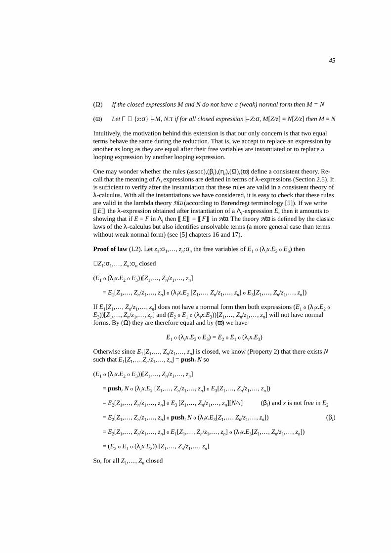
45

(Ω) If the closed expressions M and N do not have a (weak) normal form then M = N

(ω) LetΓ ∪ z:σ |−M, N:τ if for all closed expression|−Z:σ, M[Z/z] = N[Z/z] then M= N

Intuitively, the motivation behind this extension is that our only concern is that two equalterms behave the same during the reduction. That is, we accept to replace an expression byanother as long as they are equal after their free variables are instantiated or to replace alooping expression by another looping expression.

One may wonder whether the rules (assoc),(βi),(ηi),(Ω),(ω) define a consistent theory. Re-call that the meaning ofΛi expressions are defined in terms ofλ-expressions (Section 2.5). Itis sufficient to verify after the instantiation that these rules are valid in a consistent theory ofλ-calculus. With all the instantiations we have considered, it is easy to check that these rulesare valid in the lambda theoryHω (according to Barendregt terminology [5]). If we write[[ E]] the λ-expression obtained after instantiation of aΛi-expressionE, then it amounts toshowing that ifE = F in Λi then [[E]] = [[ F]] in Hω. The theoryHω is defined by the classiclaws of theλ-calculus but also identifies unsolvable terms (a more general case than termswithout weak normal form) (see [5] chapters 16 and 17).

Proof of law (L2). Let z1:σ1,…, zn:σn the free variables ofE1 o (λix.E2 o E3) then

∀Z1:σ1,…, Zn:σn closed

(E1 o (λix.E2 o E3))[Z1,…, Zn/z1,…, zn]

= E1[Z1,…, Zn/z1,…, zn] o (λix.E2 [Z1,…, Zn/z1,…, zn] o E3[Z1,…, Zn/z1,…, zn])

If E1[Z1,…, Zn/z1,…, zn] does not have a normal form then both expressions (E1 o (λix.E2 o

E3))[Z1,…, Zn/z1,…, zn] and (E2 o E1 o (λix.E3))[Z1,…, Zn/z1,…, zn] will not have normalforms. By (Ω) they are therefore equal and by (ω) we have

E1 o (λix.E2 o E3) = E2 o E1 o (λix.E3)

Otherwise sinceE1[Z1,…, Zn/z1,…, zn] is closed, we know (Property 2) that there existsNsuch thatE1[Z1,…,Zn/z1,…, zn] = pushi N so

(E1 o (λix.E2 o E3))[Z1,…, Zn/z1,…, zn]

= pushi N o (λix.E2 [Z1,…, Zn/z1,…, zn] o E3[Z1,…, Zn/z1,…, zn])

= E2[Z1,…, Zn/z1,…, zn] o E3 [Z1,…, Zn/z1,…, zn][N/x] (βi) andx is not free inE2

= E2[Z1,…, Zn/z1,…, zn] o pushi N o (λix.E3[Z1,…, Zn/z1,…, zn]) (βi)

= E2[Z1,…, Zn/z1,…, zn] o E1[Z1,…, Zn/z1,…, zn] o (λix.E3[Z1,…, Zn/z1,…, zn])

= (E2 o E1 o (λix.E3)) [Z1,…, Zn/z1,…, zn]

So, for allZ1,…, Zn closed

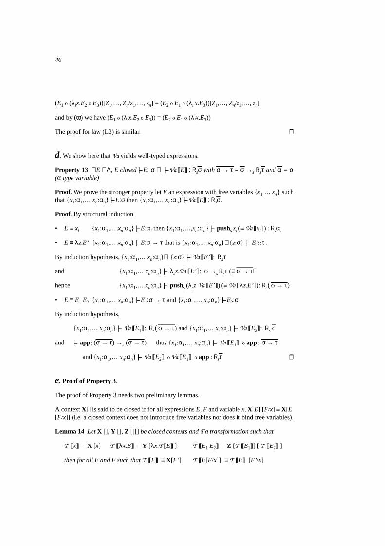
46

(E1 o (λix.E2 o E3))[Z1,…, Zn/z1,…, zn] = (E2 o E1 o (λi x.E3))[Z1,…, Zn/z1,…, zn]

and by (ω) we have (E1 o (λix.E2 o E3)) = (E2 o E1 o (λix.E3))

The proof for law (L3) is similar.

d. We show here thatVa yields well-typed expressions.

Property 13 ∀E ∈Λ, E closed|−E: σ ⇒ |−Va [[E]] : Rsσ with σ → τ = σ →s Rsτ andα = α(α type variable)

Proof. We prove the stronger property letE an expression with free variables x1 … xn suchthat x1:α1,… xn:αn |−E:σ then x1:α1,… xn:αn |−Va [[E]] : Rsσ.

Proof. By structural induction.

• E ≡ xi x1:α1,…,xn:αn |−E:αi then x1:α1,…,xn:αn |− pushsxi (≡ Va [[xi]]) : Rsαi

• E ≡ λz.E’ x1:α1,…,xn:αn |−E:σ → τ that is x1:α1,…,xn:αn ∪ z:σ |− E’::τ .

By induction hypothesis, x1:α1,… xn:αn ∪ z:σ |− Va [[E’]]: Rsτ

and x1:α1,… xn:αn |− λsz.Va [[E’]]: σ →sRsτ (≡ σ → τ)

hence x1:α1,…,xn:αn |− pushs(λsz.Va [[E’]]) (≡ Va [[λz.E’]]): Rs( σ → τ)

• E ≡ E1 E2 x1:α1,… xn:αn |−E1:σ → τ and x1:α1,… xn:αn |−E2:σ

By induction hypothesis,

x1:α1,… xn:αn |− Va [[E1]]: Rs( σ → τ) and x1:α1,… xn:αn |− Va [[E2]]: Rs σ

and |− app: (σ → τ) →s (σ → τ) thus x1:α1,… xn:αn |− Va [[E1]] o app : σ → τ

and x1:α1,… xn:αn |− Va [[E2]] o Va [[E1]] o app : Rsτ

e. Proof of Property 3.

The proof of Property 3 needs two preliminary lemmas.

A contextX[] is said to be closed if for all expressionsE, F and variablex, X[E] [F/x] ≡ X[E[F/x]] (i.e. a closed context does not introduce free variables nor does it bind free variables).

Lemma 14 LetX [], Y [], Z [][] be closed contexts andT a transformation such that

T [[x]] = X [x] T [[λx.E]] = Y [λx.T [[E]] ] T [[E1 E2]] = Z [T [[E1]]] [ T [[E2]] ]

then for all E and F such thatT [[F]] ≡ X[F’ ] T [[E[F/x]]] ≡ T [[E]] [ F’ /x]

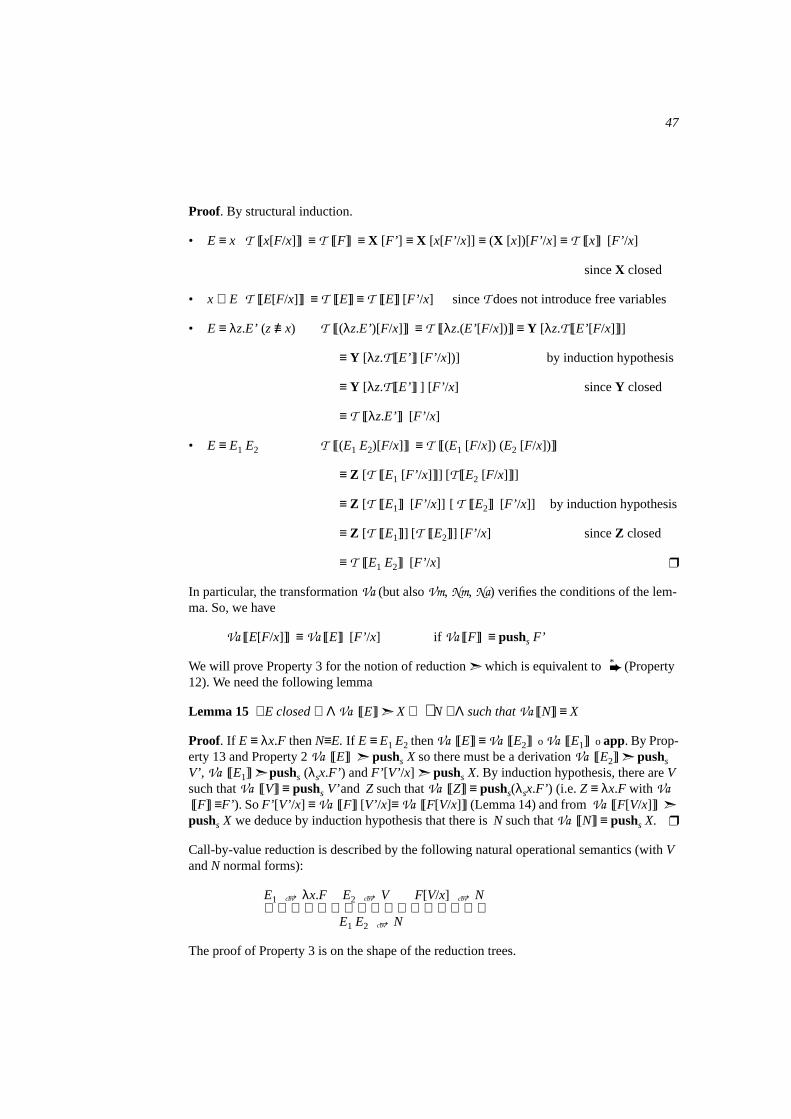
47

Proof. By structural induction.

• E ≡ x T [[x[F/x]]] ≡ T [[F]] ≡ X [F’ ] ≡ X [x[F’ /x]] ≡ (X [x])[F’ /x] ≡ T [[x]] [ F’ /x]

sinceX closed

• x ∉ E T [[E[F/x]]] ≡ T [[E]] ≡ T [[E]] [ F’ /x] sinceT does not introduce free variables

• E ≡ λz.E’ (z ≡/ x) T [[(λz.E’)[F/x]]] ≡ T [[λz.(E’[F/x])]] ≡ Y [λz.T [[E’[F/x]]]]

≡ Y [λz.T [[E’]] [ F’ /x])] by induction hypothesis

≡ Y [λz.T [[E’]] ] [ F’ /x] sinceY closed

≡ T [[λz.E’]] [ F’ /x]

• E ≡ E1 E2 T [[(E1 E2)[F/x]]] ≡ T [[(E1 [F/x]) (E2 [F/x])]]

≡ Z [T [[E1 [F’ /x]]]] [ T [[E2 [F/x]]]]

≡ Z [T [[E1]] [ F’ /x]] [ T [[E2]] [ F’ /x]] by induction hypothesis

≡ Z [T [[E1]]] [ T [[E2]]] [ F’ /x] sinceZ closed

≡ T [[E1 E2]] [ F’ /x]

In particular, the transformationVa (but alsoVm, Nm, Na) verifies the conditions of the lem-ma. So, we have

Va [[E[F/x]]] ≡ Va [[E]] [ F’ /x] if Va [[F]] ≡ pushs F’

We will prove Property 3 for the notion of reduction which is equivalent to* (Property

12). We need the following lemma

Lemma 15 ∀E closed∈ Λ Va [[E]] X ⇒ ∃N ∈Λ such thatVa [[N]] ≡ X

Proof. If E ≡ λx.F thenN≡E. If E ≡ E1 E2 thenVa [[E]] ≡ Va [[E2]] o Va [[E1]] o app. By Prop-erty 13 and Property 2Va [[E]] pushs X so there must be a derivationVa [[E2]] pushsV’, Va [[E1]] pushs (λsx.F’ ) andF’ [V’/x] pushs X. By induction hypothesis, there areVsuch thatVa [[V]] ≡ pushs V’ and Z such thatVa [[Z]] ≡ pushs(λsx.F’ ) (i.e.Z ≡ λx.F with Va[[F]] ≡F’ ). SoF’ [V’/x] ≡ Va [[F]] [ V’/x]≡ Va [[F[V/x]]] (Lemma 14) and fromVa [[F[V/x]]] pushs X we deduce by induction hypothesis that there isN such thatVa [[N]] ≡ pushs X.

Call-by-value reduction is described by the following natural operational semantics (withVandN normal forms):

E1 cbv→ λx.F E2 cbv→ V F[V/x] cbv→ N

E1 E2 cbv→ N

The proof of Property 3 is on the shape of the reduction trees.

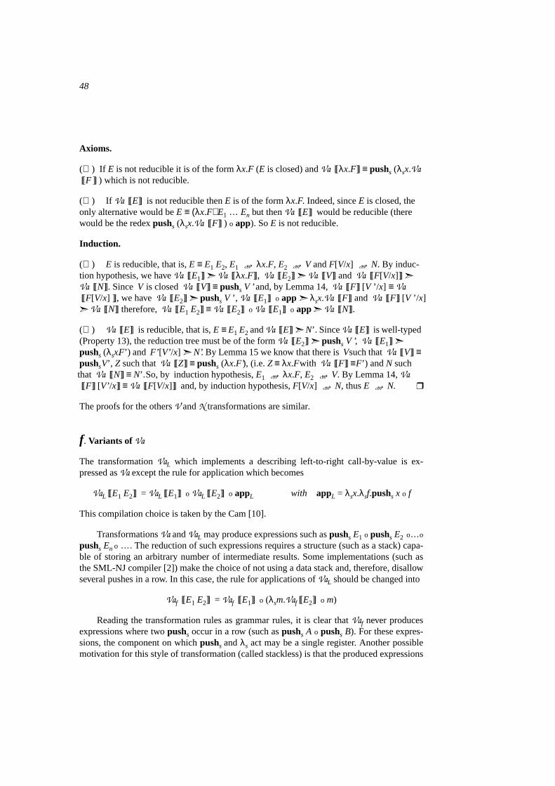
48

Axioms.

(⇒) If E is not reducible it is of the formλx.F (E is closed) andVa [[λx.F]] ≡ pushs (λsx.Va[[F ]] ) which is not reducible.

(⇐) If Va [[E]] is not reducible thenE is of the formλx.F. Indeed, sinceE is closed, theonly alternative would beE ≡ (λx.F) E1 … En but thenVa [[E]] would be reducible (therewould be the redexpushs (λsx.Va [[F]] ) o app). SoE is not reducible.

Induction.

(⇒) E is reducible, that is,E ≡ E1 E2, E1 cbv→ λx.F, E2 cbv→ V andF[V/x] cbv→ N. By induc-tion hypothesis, we haveVa [[E1]] Va [[λx.F]], Va [[E2]] Va [[V]] and Va [[F[V/x]]] Va [[N]]. Since V is closedVa [[V]] ≡ pushs V ’ and, by Lemma 14,Va [[F]] [ V ’/x] ≡ Va[[F[V/x] ]], we have Va [[E2]] pushs V ’, Va [[E1]] o app λsx.Va [[F]] and Va [[F]] [ V ’/x] Va [[N]] therefore,Va [[E1 E2]] ≡ Va [[E2]] o Va [[E1]] o app Va [[N]].

(⇐) Va [[E]] is reducible, that is,E ≡ E1 E2 andVa [[E]] N’. SinceVa [[E]] is well-typed(Property 13), the reduction tree must be of the formVa [[E2]] pushs V ’, Va [[E1]] pushs (λsx.F’) and F’ [V’/x] N’. By Lemma 15 we know that there isV such thatVa [[V]] ≡pushsV’, Z such thatVa [[Z]] ≡ pushs (λx.F’), (i.e.Z ≡ λx.F with Va [[F]] ≡F’) andN suchthat Va [[N]] ≡ N’.So, by induction hypothesis,E1 cbv→ λx.F, E2 cbv→ V. By Lemma 14,Va[[F]] [ V’/x]] ≡ Va [[F[V/x]]] and, by induction hypothesis,F[V/x] cbv→ N, thusE cbv→ N.

The proofs for the othersV andN transformations are similar.

f. Variants of Va

The transformationVaL which implements a describing left-to-right call-by-value is ex-pressed asVa except the rule for application which becomes

VaL [[E1 E2]] = VaL [[E1]] o VaL [[E2]] o appL with appL = λsx.λsf.pushs x o f

This compilation choice is taken by the Cam [10].

TransformationsVa andVaL may produce expressions such aspushs E1 o pushs E2 o…o

pushs En o …. The reduction of such expressions requires a structure (such as a stack) capa-ble of storing an arbitrary number of intermediate results. Some implementations (such asthe SML-NJ compiler [2]) make the choice of not using a data stack and, therefore, disallowseveral pushes in a row. In this case, the rule for applications ofVaL should be changed into

Vaf [[E1 E2]] = Vaf [[E1]] o (λsm.Vaf [[E2]] o m)

Reading the transformation rules as grammar rules, it is clear thatVaf never producesexpressions where twopushs occur in a row (such aspushs A o pushs B). For these expres-sions, the component on whichpushs andλs act may be a single register. Another possiblemotivation for this style of transformation (called stackless) is that the produced expressions

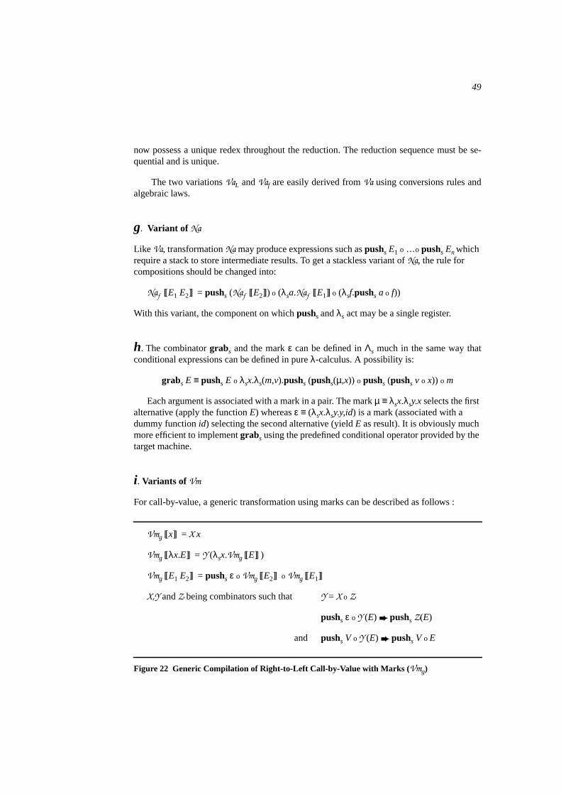
49

now possess a unique redex throughout the reduction. The reduction sequence must be se-quential and is unique.

The two variationsVaL andVaf are easily derived fromVa using conversions rules andalgebraic laws.

g. Variant of Na

Like Va, transformationNa may produce expressions such aspushs E1 o …o pushs En whichrequire a stack to store intermediate results. To get a stackless variant ofNa, the rule forcompositions should be changed into:

Naf [[E1 E2]] = pushs (Naf [[E2]]) o (λsa.Naf [[E1]] o (λsf.pushs a o f))

With this variant, the component on whichpushs andλs act may be a single register.

h. The combinatorgrabs and the markε can be defined inΛs much in the same way thatconditional expressions can be defined in pureλ-calculus. A possibility is:

grabs E ≡ pushs E o λsx.λs(m,v).pushs (pushs(µ,x)) o pushs (pushs v o x)) o m

Each argument is associated with a mark in a pair. The markµ ≡ λsx.λsy.x selects the firstalternative (apply the functionE) whereasε ≡ (λsx.λsy.y,id) is a mark (associated with adummy functionid) selecting the second alternative (yieldE as result). It is obviously muchmore efficient to implementgrabs using the predefined conditional operator provided by thetarget machine.

i. Variants of Vm

For call-by-value, a generic transformation using marks can be described as follows :

Vmg [[x]] = X x

Vmg [[λx.E]] = Y (λsx.Vmg [[E]] )

Vmg [[E1 E2]] = pushs ε o Vmg [[E2]] o Vmg [[E1]]

X,Y andZ being combinators such that Y = X o Z

pushs ε o Y (E) pushs Z(E)

and pushs V o Y (E) pushs V o E

Figure 22 Generic Compilation of Right-to-Left Call-by-Value with Marks (Vmg)

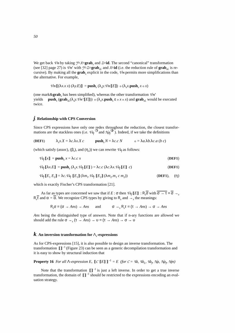
50

We get backVm by takingY=X=grabs andZ=id. The second “canonical” transformation(see [32] page 27) isVm’ with Y=Z=grabsL andX=id (i.e. the reduction rule ofgrabsL is re-cursive). By making all thegrabs explicit in the code,Vm permits more simplifications thanthe alternative. For example,

Vm [[(λx.x x) (λy.E)]] = pushs (λsy.Vm [[E]]) o (λsx.pushs x o x)

(one mark&grabs has been simplified), whereas the other transformationVm’yields pushs (grabsL(λsy.Vm’ [[E]])) o (λsx.pushs ε o x o x) andgrabsL would be executedtwice.

j. Relationship with CPS Conversion

Since CPS expressions have only one redex throughout the reduction, the closest transfor-mations are the stackless ones (i.e.Vaf

f and Nafg ). Indeed, if we take the definitions

(DEF1) λsx.X = λc.λx.X c pushsN = λc.c N o = λa.λb.λc.a (b c)

(which satisfy (assoc), (βs), and (ηs)) we can rewriteVaf as follows:

Vaf [[x]] = pushs x = λc.c x (DEF1)

Vaf [[λx.E]] = pushs (λsx.Vaf [[E]] ) = λc.c (λc.λx.Vaf [[E]] c) (DEF1)

Vaf [[E1 E2]] = λc.Vaf [[E1]] (λm1.Vaf [[E2]] (λm2.m1 c m2)) (DEF1), (η)

which is exactly Fischer’s CPS transformation [21].

As far as types are concerned we saw that ifE : σ thenVaf [[E]] : Rsσ with σ → τ = σ →sRsτ andα = α. We recognize CPS types by giving toRs and→s the meanings:

Rsσ = (σ → Ans) → Ans and σ →s Rsτ = (τ → Ans) → σ → Ans

Ans being the distinguished type of answers. Note that if n-ary functions are allowed weshould add the ruleσ →s (τ → Ans) → υ = (τ → Ans) → σ → υ

k. An inversion transformation for Λs-expressions

As for CPS-expressions [15], it is also possible to design an inverse transformation. Thetransformation [[]]-1 (Figure 23) can be seen as a generic decompilation transformation andit is easy to show by structural induction that

Property 16 For all Λ-expression E,[[C [[E]] ]] -1 = E (for C = Va, VaL, Vaf, Na, Naf, Nm)

Note that the transformation [[]]-1 is just a left inverse. In order to get a true inversetransformation, the domain of [[]]-1 should be restricted to the expressions encoding an eval-uation strategy.

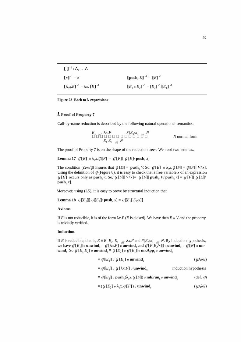
51

[[ ]] -1 : Λs → Λ

[[x]] -1 = x [[pushs E]] -1 = [[E]] -1

[[λsx.E]] -1 = λx. [[E]] -1 [[E1 o E2]]-1 = [[E2]]

-1 [[E1]]-1

Figure 23 Back toλ-expressions

l. Proof of Property 7

Call-by-name reduction is described by the following natural operational semantics:

E1 cbn→ λx.F F[E2/x]

cbn→ N

N normal formE1 E2 cbn

→ N

The proof of Property 7 is on the shape of the reduction trees. We need two lemmas.

Lemma 17 G [[E]] o λsx.G [[F]] = G [[F]][ G [[E]]/ pushs x]

The condition (CondG) insures thatG [[E]] = pushs V. So,G [[E]] o λsx.G [[F]] = G [[F]][ V/ x].Using the definition ofG (Figure 8), it is easy to check that a free variablex of an expressionG [[E]] occurs only aspushs x. So,G [[F]][ V/ x]= G [[F]][ pushs V/ pushs x] = G [[F]][ G [[E]]/pushs x].

Moreover, using (L5), it is easy to prove by structural induction that

Lemma 18 G [[E1]][ G [[E2]]/ pushs x] = G [[E1[ E2/x]]]

Axioms.

If E is not reducible, it is of the formλx.F (E is closed). We have thenE ≡ V and the propertyis trivially verified.

Induction.

If E is reducible, that is,E ≡ E1 E2, E1 cbn→ λx.F andF[E2/x]

cbn→ N. By induction hypothesis,

we haveG [[E1]] o unwinds = G [[λx.F]] o unwinds andG [[F[E2/x]]] o unwinds = G [[N]] o un-winds. SoG [[E1 E2]] o unwinds ≡ G [[E2]] o G [[E1]] o mkApp s o unwinds

= G [[E2]] o G [[E1]] o unwinds (GNm3)

= G [[E2]] o G [[λx.F]] o unwinds induction hypothesis

≡ G [[E2]] o pushs(λsx.G [[F]]) o mkFunso unwinds (def.G)

= (G [[E2]] o λsx.G [[F]]) o unwinds (GNm2)

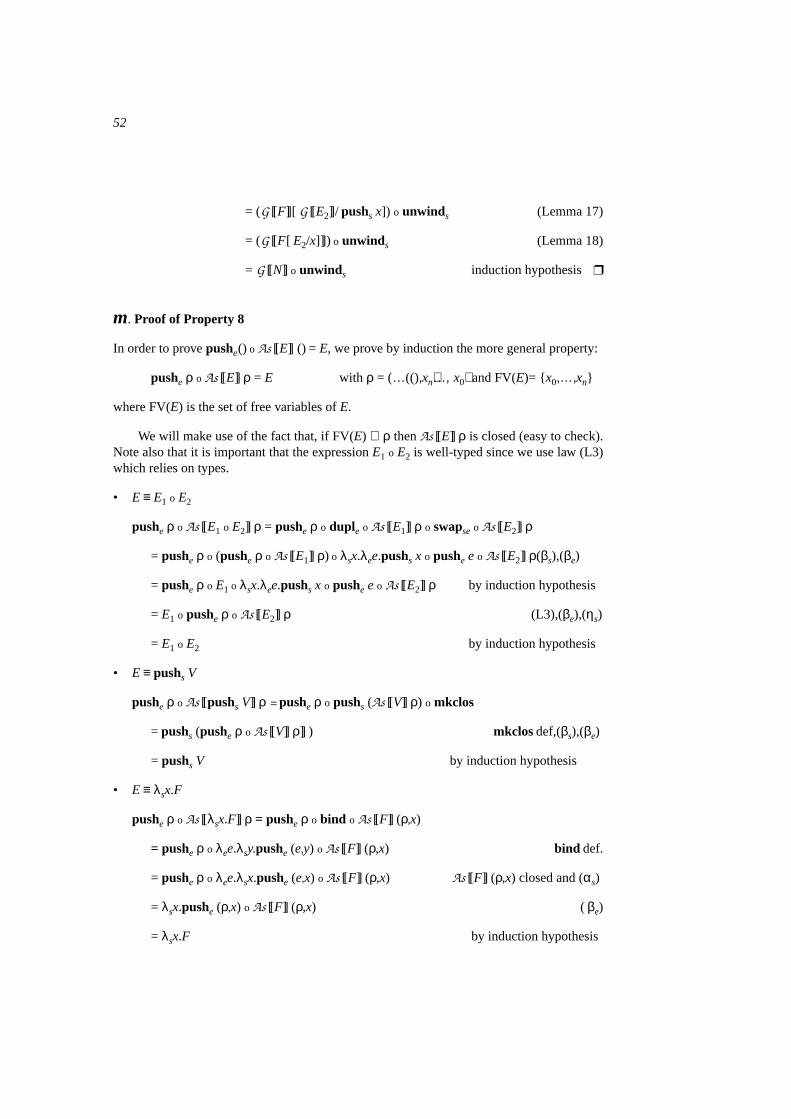
52

= (G [[F]][ G [[E2]]/ pushs x]) o unwinds (Lemma 17)

= (G [[F[ E2/x]]]) o unwinds (Lemma 18)

= G [[N]] o unwinds induction hypothesis

m. Proof of Property 8

In order to provepushe() o As [[E]] () = E, we prove by induction the more general property:

pushe ρ o As [[E]] ρ = E with ρ = (…((),xn)…,x0) and FV(E)= x0,…,xn

where FV(E) is the set of free variables ofE.

We will make use of the fact that, if FV(E) ⊆ ρ thenAs [[E]] ρ is closed (easy to check).Note also that it is important that the expressionE1 o E2 is well-typed since we use law (L3)which relies on types.

• E ≡ E1 o E2

pushe ρ o As [[E1 o E2]] ρ = pushe ρ o duple o As [[E1]] ρ o swapseo As [[E2]] ρ

= pushe ρ o (pushe ρ o As [[E1]] ρ) o λsx.λee.pushs x o pushe e o As [[E2]] ρ(βs),(βe)

= pushe ρ o E1 o λsx.λee.pushs x o pushe e o As [[E2]] ρ by induction hypothesis

= E1 o pushe ρ o As [[E2]] ρ (L3),(βe),(ηs)

= E1 o E2 by induction hypothesis

• E ≡ pushs V

pushe ρ o As [[pushs V]] ρ = pushe ρ o pushs (As [[V]] ρ) o mkclos

= pushs (pushe ρ o As [[V]] ρ]] ) mkclosdef,(βs),(βe)

= pushs V by induction hypothesis

• E ≡ λsx.F

pushe ρ o As [[λsx.F]] ρ = pushe ρ o bind o As [[F]] (ρ,x)

= pushe ρ o λee.λsy.pushe (e,y) o As [[F]] (ρ,x) bind def.

= pushe ρ o λee.λsx.pushe (e,x) o As [[F]] (ρ,x) As [[F]] (ρ,x) closed and (αs)

= λsx.pushe (ρ,x) o As [[F]] (ρ,x) ( βe)

= λsx.F by induction hypothesis

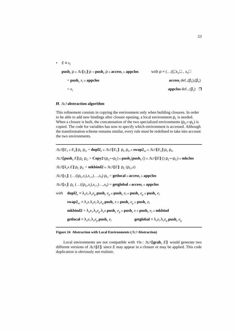
53

• E ≡ xi

pushs ρ o As [[xi]] ρ = pushe ρ o accessi o appclos with ρ = (…((),xn)…,x0)

= pushs xi o appclos accessi def.,(βs),(βe)

= xi appclosdef., (βs)

n. Ac3 abstraction algorithm

This refinement consists in copying the environment only when building closures. In orderto be able to add new bindings after closure opening, a local environmentρL is needed.When a closure is built, the concatenation of the two specialized environments (ρG++ρL) iscopied. The code for variables has now to specify which environment is accessed. Althoughthe transformation scheme remains similar, every rule must be redefined to take into accountthe two environments.

Ac3 [[E1 o E2]] ρL ρG = dupl2e o Ac3 [[E1]] ρL ρG o swap2seo Ac3 [[E2]] ρL ρG

Ac3 [[pushs E]] ρL ρG = Copy2(ρG++ρL) o pushs(pushe () o Ac3 [[E]] () ρL++ρG) o mkclos

Ac3 [[λsx.E]] ρL ρG = mkbind2 o Ac3 [[E]] ρL (ρG,x)

Ac3 [[xi]] (…((ρL,xi),xi-1)…,x0) ρG = getlocalo accessi o appclos

Ac3 [[xi]] ρL (…((ρG,xi),xi-1)…,x0) = getglobalo accessi o appclos

with dupl2e = λeel.λeeg.pushe eg o pushe el o pushe eg o pushe el

swap2se = λsx.λeel.λeeg.pushs x o pushe eg o pushe el

mkbind2 = λeel.λeeg.λsx.pushe eg o pushs x o pushe el o mkbind

getlocal= λeel.λeeg.pushe el getglobal= λeel.λeeg.pushe eg

Figure 24 Abstraction with Local Environments (Ac3 Abstraction)

Local environments are not compatible withVm : Ac3 [[grabs E]] would generate twodifferent versions ofAc3 [[E]] sinceE may appear in a closure or may be applied. This codeduplication is obviously not realistic.

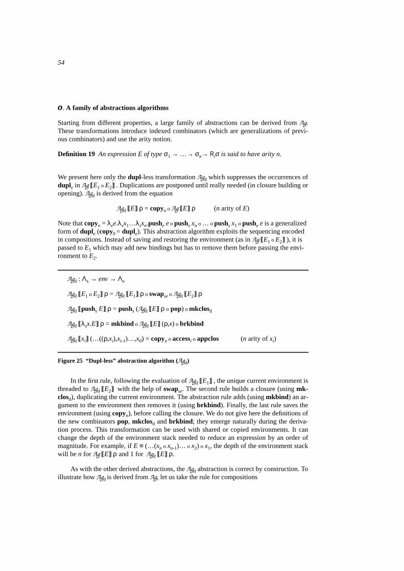
54

o. A family of abstractions algorithms

Starting from different properties, a large family of abstractions can be derived fromAg.These transformations introduce indexed combinators (which are generalizations of previ-ous combinators) and use the arity notion.

Definition 19 An expression E of typeσ1 → …→ σn→ Riσ is said to have arity n.

We present here only thedupl-less transformationAgd which suppresses the occurrences ofduple in Ag [[E1 o E2]] . Duplications are postponed until really needed (in closure building oropening).Agd is derived from the equation

Agd [[E]] ρ = copyn o Ag [[E]] ρ (n arity ofE)

Note thatcopyn = λee.λsx1…λsxn.pushe e opushs xn o… opushs x1 opushe e is a generalizedform of duple (copy0 = duple). This abstraction algorithm exploits the sequencing encodedin compositions. Instead of saving and restoring the environment (as inAg [[E1 o E2]] ), it ispassed toE1 which may add new bindings but has to remove them before passing the envi-ronment toE2.

Agd : Λs → env→ Λe

Agd [[E1 o E2]] ρ = Agd [[E1]] ρ o swapse o Agd [[E2]] ρ

Agd [[pushs E]] ρ = pushs (Agd [[E]] ρ o pop) o mkclosd

Agd [[λsx.E]] ρ = mkbind o Agd [[E]] (ρ,x) o brkbind

Agd [[xi]] (…((ρ,xi),xi-1)…,x0) = copyn o accessi o appclos (n arity ofxi)

Figure 25 “Dupl-less” abstraction algorithm (Agd)

In the first rule, following the evaluation ofAgd [[E1]] , the unique current environment isthreaded toAgd [[E2]] with the help ofswapse. The second rule builds a closure (usingmk-closd), duplicating the current environment. The abstraction rule adds (usingmkbind ) an ar-gument to the environment then removes it (usingbrkbind ). Finally, the last rule saves theenvironment (usingcopyn), before calling the closure. We do not give here the definitions ofthe new combinatorspop, mkclosd andbrkbind ; they emerge naturally during the deriva-tion process. This transformation can be used with shared or copied environments. It canchange the depth of the environment stack needed to reduce an expression by an order ofmagnitude. For example, ifE ≡ (…(xn o xn-1)… o x2) o x1, the depth of the environment stackwill be n for Ag [[E]] ρ and 1 forAgd [[E]] ρ.

As with the other derived abstractions, theAgd abstraction is correct by construction. Toillustrate howAgd is derived fromAg, let us take the rule for compositions

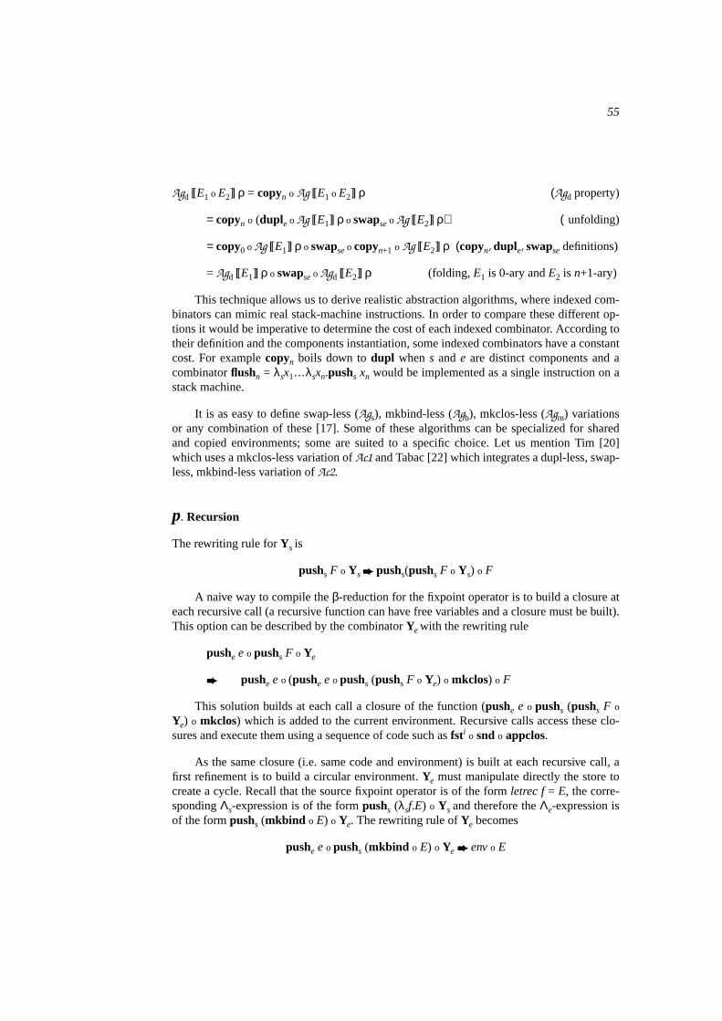
55

Agd [[E1 o E2]] ρ = copyn o Ag [[E1 o E2]] ρ (Agd property)

= copyn o (duple o Ag [[E1]] ρ o swapse o Ag [[E2]] ρ) (unfolding)

= copy0 o Ag [[E1]] ρ o swapse o copyn+1 o Ag [[E2]] ρ (copyn, duple, swapse definitions)

= Agd [[E1]] ρ o swapse o Agd [[E2]] ρ (folding, E1 is 0-ary andE2 is n+1-ary)

This technique allows us to derive realistic abstraction algorithms, where indexed com-binators can mimic real stack-machine instructions. In order to compare these different op-tions it would be imperative to determine the cost of each indexed combinator. According totheir definition and the components instantiation, some indexed combinators have a constantcost. For examplecopyn boils down todupl whens ande are distinct components and acombinatorflushn = λsx1…λsxn.pushs xn would be implemented as a single instruction on astack machine.

It is as easy to define swap-less (Ags), mkbind-less (Agb), mkclos-less (Agm) variationsor any combination of these [17]. Some of these algorithms can be specialized for sharedand copied environments; some are suited to a specific choice. Let us mention Tim [20]which uses a mkclos-less variation ofAc1 and Tabac [22] which integrates a dupl-less, swap-less, mkbind-less variation ofAc2.

p. Recursion

The rewriting rule forYs is

pushs F o Ys pushs(pushs F o Ys) o F

A naive way to compile theβ-reduction for the fixpoint operator is to build a closure ateach recursive call (a recursive function can have free variables and a closure must be built).This option can be described by the combinatorYewith the rewriting rule

pushe e o pushs F o Ye

pushe e o (pushe e o pushs (pushs F o Ye) o mkclos) o F

This solution builds at each call a closure of the function (pushe e o pushs (pushs F o

Ye) o mkclos) which is added to the current environment. Recursive calls access these clo-sures and execute them using a sequence of code such asfsti o sndo appclos.

As the same closure (i.e. same code and environment) is built at each recursive call, afirst refinement is to build a circular environment.Ye must manipulate directly the store tocreate a cycle. Recall that the source fixpoint operator is of the formletrec f= E, the corre-spondingΛs-expression is of the formpushs (λsf.E) o Ys and therefore theΛe-expression isof the formpushs (mkbind o E) o Ye. The rewriting rule ofYe becomes

pushe e o pushs (mkbind o E) o Ye envo E

56

with env = pushe e o (pushe env o pushs E o mkclos) o mkbind

The closure (pushe env o pushs E o mkclos) is built only once for each series of recur-sive calls (note that the initialmkbind has been suppressed). The circular environmentenvof this closure is made of the environment of the recursive function and the closure itself.When accessing the closure, circularity makes the code reinstall the environmentenv forfree.

A second refinement used in environment based machines is to implement recursivecalls to statically known functions by a jump to their address. It is sufficient to replace a re-cursive callfsti o sndo appclos by fsti o E. A recursive call is not anymore the evaluation ofa closure, but consists in installing the environment (i.e. the free variables) of the function(fsti) and calling its code (E). Of course, in order to get a real code machine, this call shouldbe implemented by a jump to a label. With this solution, recursive functions appear in clo-sures only when they are passed as argument.