A System-Level Framework for Energy and Performance Estimation
146
A System-Level Framework for Energy and Performance Estimation of System-on-Chip Architectures SANDRO PENOLAZZI Doctoral Thesis in Electronic and Computer Systems Stockholm, Sweden 2011
Transcript of A System-Level Framework for Energy and Performance Estimation
A System-Level Framework for Energy andPerformance Estimation of System-on-Chip
Architectures
SANDRO PENOLAZZI
Doctoral Thesis in Electronic and Computer SystemsStockholm, Sweden 2011
TRITA-ICT/ECS AVH 11:02ISSN 1653-6363ISRN KTH/ICT/ECS/AVH-11/02-SEISBN 978-91-7415-881-6
KTH School of Information andCommunication Technology
SE-164 40 KistaSWEDEN
Akademisk avhandling som med tillstånd av Kungl Tekniska högskolan framläggestill offentlig granskning för avläggande av teknologie doktorsexamen onsdagen den6 april 2011 klockan 13.00 i Sal C1, Electrum, Isafjordsgatan 26, Kista.
© Sandro Penolazzi, April 2011
Tryck: Universitetsservice US AB
iii
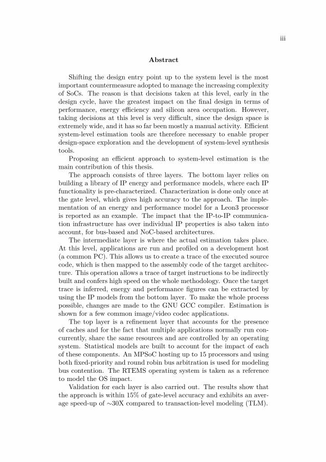
Abstract
Shifting the design entry point up to the system level is the mostimportant countermeasure adopted to manage the increasing complexityof SoCs. The reason is that decisions taken at this level, early in thedesign cycle, have the greatest impact on the final design in terms ofperformance, energy efficiency and silicon area occupation. However,taking decisions at this level is very difficult, since the design space isextremely wide, and it has so far been mostly a manual activity. Efficientsystem-level estimation tools are therefore necessary to enable properdesign-space exploration and the development of system-level synthesistools.
Proposing an efficient approach to system-level estimation is themain contribution of this thesis.
The approach consists of three layers. The bottom layer relies onbuilding a library of IP energy and performance models, where each IPfunctionality is pre-characterized. Characterization is done only once atthe gate level, which gives high accuracy to the approach. The imple-mentation of an energy and performance model for a Leon3 processoris reported as an example. The impact that the IP-to-IP communica-tion infrastructure has over individual IP properties is also taken intoaccount, for bus-based and NoC-based architectures.
The intermediate layer is where the actual estimation takes place.At this level, applications are run and profiled on a development host(a common PC). This allows us to create a trace of the executed sourcecode, which is then mapped to the assembly code of the target architec-ture. This operation allows a trace of target instructions to be indirectlybuilt and confers high speed on the whole methodology. Once the targettrace is inferred, energy and performance figures can be extracted byusing the IP models from the bottom layer. To make the whole processpossible, changes are made to the GNU GCC compiler. Estimation isshown for a few common image/video codec applications.
The top layer is a refinement layer that accounts for the presenceof caches and for the fact that multiple applications normally run con-currently, share the same resources and are controlled by an operatingsystem. Statistical models are built to account for the impact of eachof these components. An MPSoC hosting up to 15 processors and usingboth fixed-priority and round robin bus arbitration is used for modelingbus contention. The RTEMS operating system is taken as a referenceto model the OS impact.
Validation for each layer is also carried out. The results show thatthe approach is within 15% of gate-level accuracy and exhibits an aver-age speed-up of ∼30X compared to transaction-level modeling (TLM).


Acknowledgments
Stockholm, February 2011
I would like first of all to thank my supervisor, Professor Ahmed Hemani. He hasalways been very present and supported me with his valuable advice and knowledge,especially at the beginning of my PhD, when the path to take still looked uncertain.A great thank you also goes to Ingo Sander, who accepted to be my co-supervisorduring the second half of my PhD and who has always given me very useful guidance.
I am very thankful to all my colleagues and friends that shared part of the lastfive years with me at the department. A warm thanks to Haider Abbas, DavideCalusini, Dr. Zhonghai Lu, Omer Malik, Ali Shami, Adeel Tajammul and ChenZhipeng for the nice conversations we had, always a valid excuse to take a break.I am particularly grateful to Mohammad Badawi, Luca Bolognino and Bin Liu:each of them has helped me in a different phase of my research and it is also inpart thanks to them if the accomplishment of this PhD thesis has been possible.I also want to thank Jean-Michel Chabloz and Shohreh Sharif Mansouri, two dearfriends with whom I have shared my thoughts, worries and moments of joy. Thankyou also to Jun Zhu for helping me with the practicalities related to the process ofhanding in the thesis.
I am very grateful to my parents whom, despite the distance, I have always feltnear during these long five years of doctoral studies. It is thanks to their supportand encouragement if I did not lose my motivation and if I was able to get over themany challenges that appeared on my way. Finally, I want to express my sinceregratitude to a person that has a special place in my life: thank you, Evanny, foralways staying close to me and understanding me. Your presence and your wordshave given me the energy and the optimism I needed to complete this long work.
Sandro Penolazzi
v

Contents
Contents vii
List of Tables xi
List of Figures xiii
1 Introduction 11.1 Background: the Increasing Complexity of Electronic Devices . . . . 1
1.1.1 Progress in the semiconductor industry . . . . . . . . . . . . 21.1.2 Increased applications demand . . . . . . . . . . . . . . . . . 2
1.2 System Partitioning . . . . . . . . . . . . . . . . . . . . . . . . . . . 31.3 Abstraction: from Physical to System Level . . . . . . . . . . . . . . 41.4 System-Level Estimation . . . . . . . . . . . . . . . . . . . . . . . . . 51.5 Thesis Contribution . . . . . . . . . . . . . . . . . . . . . . . . . . . 81.6 Thesis Layout . . . . . . . . . . . . . . . . . . . . . . . . . . . . . . . 11
2 Common Approaches to System-Level Estimation and DesignToday 132.1 Introduction . . . . . . . . . . . . . . . . . . . . . . . . . . . . . . . . 132.2 Simulation-Based Estimation Tools . . . . . . . . . . . . . . . . . . . 14
2.2.1 An overview of SystemC and Transaction Level Modeling(TLM) . . . . . . . . . . . . . . . . . . . . . . . . . . . . . . . 21
2.2.2 Time representation in TLM . . . . . . . . . . . . . . . . . . 232.2.3 TLM advantages . . . . . . . . . . . . . . . . . . . . . . . . . 242.2.4 TLM drawbacks . . . . . . . . . . . . . . . . . . . . . . . . . 252.2.5 Examples of SystemC/TLM usage in RTOS and MPSoCs
modeling . . . . . . . . . . . . . . . . . . . . . . . . . . . . . 262.3 Analytical Estimation Tools . . . . . . . . . . . . . . . . . . . . . . . 272.4 Estimation Tools Based on the Combination of Multiple Approaches 272.5 Which Category Does Funtime Belong to? . . . . . . . . . . . . . . . 28
3 An Overview of the Funtime Estimation Framework 313.1 Introduction . . . . . . . . . . . . . . . . . . . . . . . . . . . . . . . . 31
vii
viii CONTENTS
3.2 Funtime User Interface . . . . . . . . . . . . . . . . . . . . . . . . . . 323.3 Level A – The IP Level . . . . . . . . . . . . . . . . . . . . . . . . . 33
3.3.1 Level A1 – Individual IPs . . . . . . . . . . . . . . . . . . . . 333.3.2 Level A2 – Architecture of IPs . . . . . . . . . . . . . . . . . 34
3.4 Level B – The Algorithmic Level . . . . . . . . . . . . . . . . . . . . 353.4.1 Instrumentation and trace generation for applications mapped
to software . . . . . . . . . . . . . . . . . . . . . . . . . . . . 373.4.1.1 Advantages and challenges of the estimation ap-
proach for applications mapped to software . . . . . 393.4.1.2 Enhancing the GNU GCC compiler . . . . . . . . . 40
3.4.2 Estimation of applications mapped to hardware . . . . . . . . 413.5 Level C – The Refinement Level . . . . . . . . . . . . . . . . . . . . 443.6 From Single Transactions to a Final Trace . . . . . . . . . . . . . . . 473.7 Time Representation in Funtime . . . . . . . . . . . . . . . . . . . . 473.8 Engineering Effort in Funtime . . . . . . . . . . . . . . . . . . . . . . 503.9 Refinements Order and Interaction . . . . . . . . . . . . . . . . . . . 50
4 Level A1 – Implementing IP Energy and Performance Models:The Leon3 Processor Case 534.1 Introduction . . . . . . . . . . . . . . . . . . . . . . . . . . . . . . . . 534.2 Related Work . . . . . . . . . . . . . . . . . . . . . . . . . . . . . . . 544.3 Configuration and Synthesis . . . . . . . . . . . . . . . . . . . . . . . 554.4 Energy Characterization . . . . . . . . . . . . . . . . . . . . . . . . . 55
4.4.1 1-instruction-based model . . . . . . . . . . . . . . . . . . . . 564.4.2 2-instruction-based model . . . . . . . . . . . . . . . . . . . . 58
4.5 Data Switching Activity . . . . . . . . . . . . . . . . . . . . . . . . . 594.6 Registers Correlation . . . . . . . . . . . . . . . . . . . . . . . . . . . 604.7 Validating the Leon3 Model Estimation Accuracy . . . . . . . . . . 614.8 Summary . . . . . . . . . . . . . . . . . . . . . . . . . . . . . . . . . 65
5 Level A2 – Modeling IPs Composite Transactions 675.1 Introduction . . . . . . . . . . . . . . . . . . . . . . . . . . . . . . . . 675.2 Bus-based and NoC-based SoC: Architectural Similarities and Dif-
ferences . . . . . . . . . . . . . . . . . . . . . . . . . . . . . . . . . . 685.3 Characterizing Composite Transactions . . . . . . . . . . . . . . . . 695.4 Validating the Accuracy of the Extended Model for Leon3 . . . . . . 745.5 Summary . . . . . . . . . . . . . . . . . . . . . . . . . . . . . . . . . 76
6 Level B – Inferring Primary Transactions and Refinements forTransactions Interdependency and Caches 776.1 Introduction . . . . . . . . . . . . . . . . . . . . . . . . . . . . . . . . 776.2 Transactions Interdependency Refinement . . . . . . . . . . . . . . . 786.3 Validating the Algorithmic Level and the Accuracy of the Transac-
tions Interdependency Refinement . . . . . . . . . . . . . . . . . . . 80

CONTENTS ix
6.4 Cache Effect Refinement . . . . . . . . . . . . . . . . . . . . . . . . . 826.5 Comparing Funtime and Untimed TLM Estimation Speed . . . . . . 83
7 Level C – Refining Bus Contention Effects on Energy and Per-formance 857.1 Introduction . . . . . . . . . . . . . . . . . . . . . . . . . . . . . . . . 857.2 Characterizing Bus Contention . . . . . . . . . . . . . . . . . . . . . 87
7.2.1 Factor 1: number of processors . . . . . . . . . . . . . . . . . 897.2.2 Factor 2: number of w/r accesses to memory . . . . . . . . . 927.2.3 Summary . . . . . . . . . . . . . . . . . . . . . . . . . . . . . 93
7.3 Predicting Bus Contention . . . . . . . . . . . . . . . . . . . . . . . . 947.3.1 Case study . . . . . . . . . . . . . . . . . . . . . . . . . . . . 94
7.4 Validating the Accuracy of Bus Contention Prediction . . . . . . . . 967.5 Summary . . . . . . . . . . . . . . . . . . . . . . . . . . . . . . . . . 97
8 Level C – Refining the Operating System Overhead on Energyand Performance 998.1 Introduction . . . . . . . . . . . . . . . . . . . . . . . . . . . . . . . . 998.2 RTOS Characterization . . . . . . . . . . . . . . . . . . . . . . . . . 101
8.2.1 Characterizing a group of RTOS routines . . . . . . . . . . . 1018.3 RTOS Activity Prediction . . . . . . . . . . . . . . . . . . . . . . . . 103
8.3.1 Round Robin scheduler activity prediction . . . . . . . . . . . 1058.3.1.1 Case study 1 . . . . . . . . . . . . . . . . . . . . . . 1058.3.1.2 Case study 2 . . . . . . . . . . . . . . . . . . . . . . 1058.3.1.3 Case study 3 . . . . . . . . . . . . . . . . . . . . . . 107
8.3.2 Prediction of Priority-Driven Scheduler Activity . . . . . . . 1078.3.2.1 Case study 1 . . . . . . . . . . . . . . . . . . . . . . 1088.3.2.2 Case study 2 . . . . . . . . . . . . . . . . . . . . . . 110
8.4 Validation of Refinement Accuracy . . . . . . . . . . . . . . . . . . . 1138.4.1 Round Robin scheduler . . . . . . . . . . . . . . . . . . . . . 1138.4.2 Priority-driven scheduler . . . . . . . . . . . . . . . . . . . . . 114
8.5 Summary . . . . . . . . . . . . . . . . . . . . . . . . . . . . . . . . . 116
9 Conclusions and Future Work 1179.1 Conclusions . . . . . . . . . . . . . . . . . . . . . . . . . . . . . . . . 1179.2 Future Work . . . . . . . . . . . . . . . . . . . . . . . . . . . . . . . 119
Bibliography 121


List of Tables
4.1 Leon3 area . . . . . . . . . . . . . . . . . . . . . . . . . . . . . . . . . . 554.2 Leon3 LUT for energy and performance . . . . . . . . . . . . . . . . . . 574.3 Energy models: 1-instr. vs. 2-instr. . . . . . . . . . . . . . . . . . . . . . 584.4 Analysis of data switching activity . . . . . . . . . . . . . . . . . . . . . 594.5 Registers correlation analysis . . . . . . . . . . . . . . . . . . . . . . . . 614.6 Leon3 energy models (1-instr-based with/without data dependency) vs.
gate-level energy measurement (no cache) . . . . . . . . . . . . . . . . . 614.7 Leon3 energy models (1-instr-based with/without data dependency) vs.
gate-level energy measurement (4kB I/D-cache) . . . . . . . . . . . . . . 624.8 Leon3 energy models (1-instr-based/2-instr-based with data dependency)
vs. gate-level energy measurement (no cache) . . . . . . . . . . . . . . . 634.9 Leon3 energy models (1-instr-based/2-instr-based with data dependency)
vs. gate-level energy measurement (4kB I/D-cache) . . . . . . . . . . . . 64
5.1 Summary of the characterization results for simple and composite trans-actions in Leon3 (no cache) . . . . . . . . . . . . . . . . . . . . . . . . . 72
5.2 Leon3 model validation versus gate-level energy measurement . . . . . . 75
6.1 Comparison between ideal and real average cycles per instruction . . . . 816.2 2 sources of inaccuracy: Leon3 energy & performance model + estimated
number of cycles (stalls) . . . . . . . . . . . . . . . . . . . . . . . . . . . 816.3 3 sources of inaccuracy: Leon3 energy & performance model + estimated
number of cycles (stalls) + estimated number of instructions . . . . . . 826.4 Timing comparison between Funtime and untimed TLM . . . . . . . . . 84
7.1 Percentage of cycles difference C%N,1 between N and 1-processor case . . 89
7.2 Percentage of cycles difference C%N,N−1 . . . . . . . . . . . . . . . . . . . 90
7.3 Value of Estall
cycle [pJ ] calculated by Equation 7.2 for 2 ≤ N ≤ 7 . . . . . . 927.4 Percentage of instruction-level cycles difference C%
7,1 for the FFT . . . . 927.5 Average C%
wr,na,1 and C%wr,na,1 calculated on the FFT, Fibonacci and
Viterbi benchmarks . . . . . . . . . . . . . . . . . . . . . . . . . . . . . 95
xi

xii List of Tables
7.6 Measured vs. predicted execution time exi[ms] and Ei[µJ ]. 3 differentapplications on a 3-processor SoC. . . . . . . . . . . . . . . . . . . . . . 97
8.1 Energy and performance characterization for RTEMS on Leon3 (no cache)1038.2 Validating Funtime vs. gate level for energy estimation: 2 RR-scheduled
tasks of different length . . . . . . . . . . . . . . . . . . . . . . . . . . . 1148.3 Validating Funtime vs. gate level for energy estimation: priority-driven
scheduling . . . . . . . . . . . . . . . . . . . . . . . . . . . . . . . . . . . 115

List of Figures
1.1 CPU transistors count from 1971 to 2008 . . . . . . . . . . . . . . . . . 21.2 Complexity increase for newer Windows versions [44] . . . . . . . . . . 31.3 Gajski-Kuhn Y-chart . . . . . . . . . . . . . . . . . . . . . . . . . . . . . 41.4 System-level design challenge: the mapping phase . . . . . . . . . . . . . 61.5 Design space width versus abstraction level . . . . . . . . . . . . . . . . 7
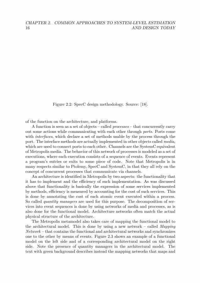
2.1 Ptolemy hierarchical model using two different domains. Source: [19]. . 152.2 SpecC design methodology. Source: [18]. . . . . . . . . . . . . . . . . . . 162.3 Mapping network in Metropolis. The functional network on the left side
and the architectural network on the right side. Source: [8]. . . . . . . . 172.4 Mapping between the application and the architecture model in SPADE.
Source: [41]. . . . . . . . . . . . . . . . . . . . . . . . . . . . . . . . . . . 182.5 Left: mapping between the application and the architecture model in
Artemis. Right: integration between DSE activity and use of reconfig-urable architectures. Source: [64]. . . . . . . . . . . . . . . . . . . . . . . 18
2.6 MILAN design, DSE and estimation framework. Source: [49]. . . . . . . 192.7 TAPES trace example. Source: [76]. . . . . . . . . . . . . . . . . . . . . 202.8 C++, SystemC and TLM relation. . . . . . . . . . . . . . . . . . . . . . 222.9 Time abstraction levels. Source: [9]. . . . . . . . . . . . . . . . . . . . . 232.10 TLM-based design flow. Figure taken from [26]. . . . . . . . . . . . . . . 25
3.1 Funtime 3-layer estimation framework . . . . . . . . . . . . . . . . . . . 323.2 Example: database of IP models A . . . . . . . . . . . . . . . . . . . . . 343.3 Example: architecture composition of IPs . . . . . . . . . . . . . . . . . 353.4 Instrumentation of applications mapped to software . . . . . . . . . . . 383.5 The GNU GCC execution flow . . . . . . . . . . . . . . . . . . . . . . . 413.6 Example of source execution trace . . . . . . . . . . . . . . . . . . . . . 413.7 Example: Applications mapped to software and hardware . . . . . . . . 433.8 Example: Real scenario including RTOS, concurrent execution and com-
petition for shared resources (bus) . . . . . . . . . . . . . . . . . . . . . 463.9 Visual representation of a single transaction . . . . . . . . . . . . . . . . 47
xiii
xiv List of Figures
3.10 From single transactions to a full trace of primary and secondary trans-actions . . . . . . . . . . . . . . . . . . . . . . . . . . . . . . . . . . . . . 48
3.11 Comparison between the time representation in TLM and Funtime . . . 483.12 First refinement: transaction interdependency . . . . . . . . . . . . . . . 51
4.1 The IP Level – Individual IPs (Level A1) . . . . . . . . . . . . . . . . . 544.2 EnIUT1+EnIUT2 versus EnIUT1_IUT2 . . . . . . . . . . . . . . . . . . . 584.3 Energy change vs. data switching activity . . . . . . . . . . . . . . . . . 594.4 Distribution of simultaneously switching bits per register . . . . . . . . 60
5.1 The IP Level – Architecture of IPs (Level A2) . . . . . . . . . . . . . . . 685.2 Leon3-based SoC Architecture . . . . . . . . . . . . . . . . . . . . . . . 685.3 Leon3-based McNoC Architecture . . . . . . . . . . . . . . . . . . . . . 695.4 Different cases considered for characterization of composite transactions 705.5 Cycles and energy statistics for the ld instruction . . . . . . . . . . . . 74
6.1 The Algorithmic Level (Level B) . . . . . . . . . . . . . . . . . . . . . . 786.2 Validating the cache refinement . . . . . . . . . . . . . . . . . . . . . . . 836.3 Cycles variation as a function of the cache miss ratio . . . . . . . . . . . 84
7.1 The Refinement Level (Level C) - Refining bus contention . . . . . . . . 867.2 Reference SoC . . . . . . . . . . . . . . . . . . . . . . . . . . . . . . . . 887.3 Execution time exi (in number of cycles) for FFT, Fibonacci and Viterbi 897.4 Execution time exi (in cycles) for FFT, 1 ≤ N ≤ 15 . . . . . . . . . . . 907.5 MPSoC execution time for N processors and N different applications . 95
8.1 The Refinement Level (Level C) – Refining the OS overhead . . . . . . . 1008.2 Leon3-based platform . . . . . . . . . . . . . . . . . . . . . . . . . . . . 1018.3 Example of an objdump output . . . . . . . . . . . . . . . . . . . . . . . 1028.4 RTOS Modeler . . . . . . . . . . . . . . . . . . . . . . . . . . . . . . . . 1028.5 RR scheduling: ∀Ti, trel,i = 0 and exi = EX . . . . . . . . . . . . . . . 1058.6 Round Robin scheduling: ∀Ti, trel,i = 0, exi 6= EX and exi 6= exj . . . . 1068.7 Round Robin scheduling: ∀Ti, trel,i 6= 0, exi 6= EX, exi 6= exj , exsc(rdy(t))
and exct(rdy(t)) . . . . . . . . . . . . . . . . . . . . . . . . . . . . . . . 1078.8 3 independent tasks T1, T2 and T3. trel,i 6= trel,j . . . . . . . . . . . . . 1098.9 3 inter-dependent tasks T1, T2, T3 and T4. trel,i 6= trel,j . . . . . . . . . 1118.10 RTEMS-based signal-processing software . . . . . . . . . . . . . . . . . . 115

List of Publications
1. S. Penolazzi, I. Sander and A. Hemani, "Estimating Bus Contention Effects onEnergy and Performance in Multi-Processor SoCs". In Proceedings of Design,Automation and Test in Europe (DATE’11), Grenoble, France, 2011.
2. S. Penolazzi, I. Sander and A. Hemani, "Predicting Energy and PerformanceOverhead of Real-Time Operating Systems". In Proceedings of Design, Au-tomation and Test in Europe (DATE’10), Dresden, Germany, 2010, pp. 15-20.
3. S. Penolazzi, I. Sander and A. Hemani, "Inferring Energy and PerformanceCost of RTOS in Priority-Driven Scheduling". In Proceedings of Symposiumon Industrial Embedded Systems (SIES’10), Trento, Italy, 2010, pp. 1-8.
4. S. Penolazzi, A. Hemani and L. Bolognino, "A General Approach to High-Level Energy and Performance Estimation in SoCs". In Proceedings of VLSIConference (VLSI’09), New Delhi, India, 2009, pp. 200-205.
5. S. Penolazzi, L. Bolognino and A. Hemani, "Energy and Performance Model ofa SPARC Leon3 Processor". In Proceedings of the 12th Euromicro Conferenceon Digital System Design (DSD’09), Patras, Greece, 2009, pp. 651-656.
6. S. Penolazzi, A. Hemani and L. Bolognino, "A General Approach to High-Level Energy and Performance Estimation in SoCs". In Journal of Low PowerElectronics (JOLPE’09), Volume 5, Number 3, October 2009, pp. 373-384.
7. S. Penolazzi, M. Badawi, and A. Hemani, "A Step Beyond TLM: InferringArchitectural Transactions at Functional Untimed Level". In Proceedings ofVLSI-SoC Conference (VLSI-SoC’08), Rhodes, Greece, 2008, pp. 505-509.
8. S. Penolazzi, A. Hemani and M. Badawi, "Modelling Embedded Systems atFunctional Untimed Application Level". In Proceedings of IP Conference(IP’07), Grenoble, France, 2007, pp. 107-112.
9. S. Penolazzi and A. Hemani, "A Layered Approach to Estimating Power Con-sumption". In Proceedings of Norchip Conference (Norchip’06), Linkoping,Sweden, 2006, pp. 93-98.
xv

xvi List of Figures
10. S. Penolazzi and A. Jantsch, "A High-Level Power Model for the NostrumNoC". In Proceedings of the 9th Euromicro Conference on Digital SystemDesign (DSD’06), August 2006, pp. 673-676.
List of Acronyms
ABS Anti-lock Braking System
API Application Programming Interface
AS Architecture Specification
CAD Computer Aided Design
CLT Central Limit Theorem
CPU Central Processing Unit
DSE Design Space Exploration
DSP Digital Signal Processor
EDA Electronic Design Automation
HDL Hardware Description Language
HLL High-Level Language
HLS High-Level Synthesis
IP Intellectual Property
IPC Inter-Process Communication
ISS Instruction-Set Simulation
ITRS International Technology Roadmap for Semiconductors
MoC Model of Computation
MPSoC Multi-Processor SoC
NoC Network on Chip
OS Operating System
xvii

xviii List of Figures
OSCI Open SystemC Initiative
PBD Platform-Based Design
RTL Register Transfer Level
RTOS Real-Time OS
SLD System-Level Design
SLE System-Level Estimation
SLOC Source Lines of Code
SoC System on Chip
TLM Transaction Level Modeling
UCS Use Case Specification
VHDL Very high speed HDL
WCET Worst-Case Execution Time
Chapter 1
Introduction
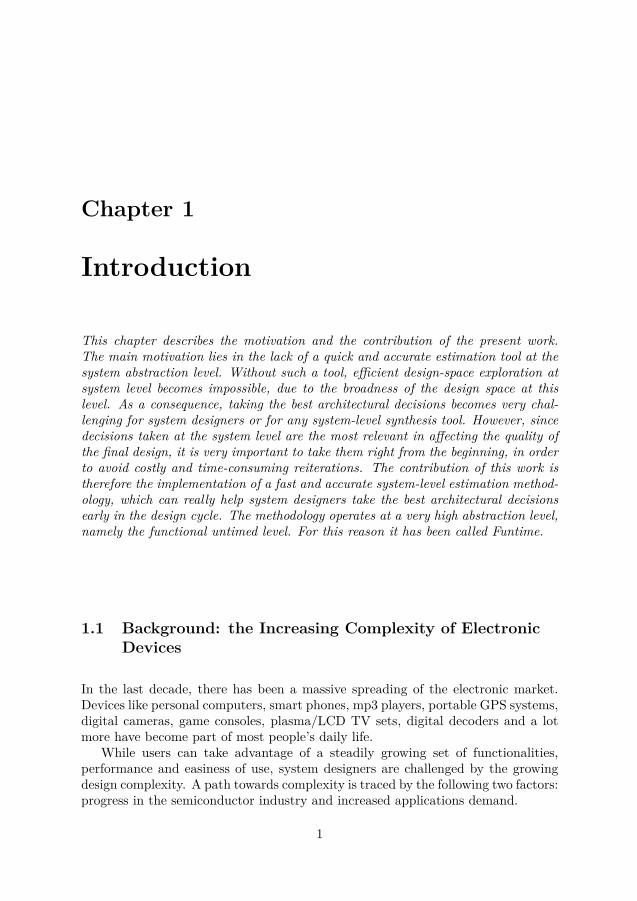
This chapter describes the motivation and the contribution of the present work.The main motivation lies in the lack of a quick and accurate estimation tool at thesystem abstraction level. Without such a tool, efficient design-space exploration atsystem level becomes impossible, due to the broadness of the design space at thislevel. As a consequence, taking the best architectural decisions becomes very chal-lenging for system designers or for any system-level synthesis tool. However, sincedecisions taken at the system level are the most relevant in affecting the quality ofthe final design, it is very important to take them right from the beginning, in orderto avoid costly and time-consuming reiterations. The contribution of this work istherefore the implementation of a fast and accurate system-level estimation method-ology, which can really help system designers take the best architectural decisionsearly in the design cycle. The methodology operates at a very high abstraction level,namely the functional untimed level. For this reason it has been called Funtime.
1.1 Background: the Increasing Complexity of ElectronicDevices
In the last decade, there has been a massive spreading of the electronic market.Devices like personal computers, smart phones, mp3 players, portable GPS systems,digital cameras, game consoles, plasma/LCD TV sets, digital decoders and a lotmore have become part of most people’s daily life.
While users can take advantage of a steadily growing set of functionalities,performance and easiness of use, system designers are challenged by the growingdesign complexity. A path towards complexity is traced by the following two factors:progress in the semiconductor industry and increased applications demand.
1
2 CHAPTER 1. INTRODUCTION
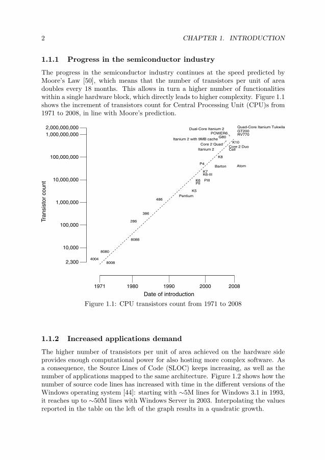
1.1.1 Progress in the semiconductor industryThe progress in the semiconductor industry continues at the speed predicted byMoore’s Law [50], which means that the number of transistors per unit of areadoubles every 18 months. This allows in turn a higher number of functionalitieswithin a single hardware block, which directly leads to higher complexity. Figure 1.1shows the increment of transistors count for Central Processing Unit (CPU)s from1971 to 2008, in line with Moore’s prediction.
Figure 1.1: CPU transistors count from 1971 to 2008
1.1.2 Increased applications demandThe higher number of transistors per unit of area achieved on the hardware sideprovides enough computational power for also hosting more complex software. Asa consequence, the Source Lines of Code (SLOC) keeps increasing, as well as thenumber of applications mapped to the same architecture. Figure 1.2 shows how thenumber of source code lines has increased with time in the different versions of theWindows operating system [44]: starting with ∼5M lines for Windows 3.1 in 1993,it reaches up to ∼50M lines with Windows Server in 2003. Interpolating the valuesreported in the table on the left of the graph results in a quadratic growth.

1.2. SYSTEM PARTITIONING 3
1992 1994 1996 1998 2000 2002 20040
10
20
30
40
50
60 YearMillionsofsourcecodelinesFigure 1.2: Complexity increase for newer Windows versions [44]
1.2 System Partitioning
Design partitioning is one of the two main countermeasures taken to manage thegrowing complexity. In general, this concept relies on the idea that one problemcan be simplified by decomposing it in several smaller sub-problems. When appliedto VLSI design, this means that a design is no longer seen as a whole flat sea oftransistors; instead, it is considered as an aggregate of smaller and hierarchicalsub-designs connected together. Multiple layers of hierarchy may coexist and eachsub-design is normally representative of a certain functionality. In other words, hi-erarchy helps reduce complexity by hiding it within each sub-system block/module.Note that the partitioning process is a manual activity.
As complexity increases, so does the granularity of the basic building blocks. Inaddition, the trend goes towards a standardization of very commonly used blocks,which are usually known as Intellectual Property (IP)s. Examples of IPs are micro-processors, DSP cores, codecs, modems, etc. Such IPs are taken from a library andused as black boxes to build new system architectures, thus being a fundamentalhelp in reducing design complexity and improving the time to market. Buildingnew components from scratch is in fact very time consuming and expensive.
A further increase in the partitioning granularity has led to an extension of theIP concept and has led to the introduction of the Platform-Based Design (PBD)term. PBD goes beyond the standardization of individual IPs and proposes insteadthe standardization of entire platforms. Although different interpretations of PBDexist, the following definition given by Alberto Sangiovanni-Vincentelli can be takenas an example: a platform is “a layer of abstraction with two views: the upper viewis the abstraction of the design below so that an application could be developedon the abstraction without referring to the lower levels of abstraction. The lowerview is the set of rules that integrates components as part of the platform.” Thisdefinition suggests that a platform can be seen as an Application ProgrammingInterface (API), thus allowing applications to be written without caring about theactual underlying architecture, as long as the interface rules are followed.
4 CHAPTER 1. INTRODUCTION
1.3 Abstraction: from Physical to System Level
The second countermeasure taken to manage complexity is raising the design ab-straction level. While design partitioning reduces complexity by basically hidingit in each subsystem block, raising the design abstraction eliminates complexity,in the sense that automatic tools, known as Electronic Design Automation (EDA)tools, are normally developed to automatically deal with it through a process calledsynthesis. In other words, synthesis automatically accounts for complexity by trans-lating a description made by the designer at a certain abstraction level into a lowerlevel. Note that the increase of granularity proposed by system partitioning andthe increase of abstraction usually go in parallel.
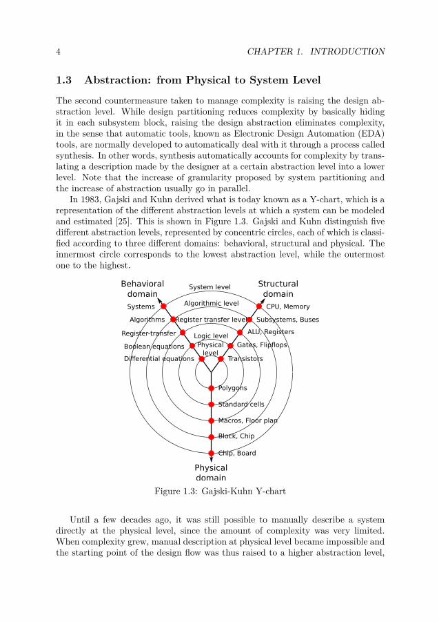
In 1983, Gajski and Kuhn derived what is today known as a Y-chart, which is arepresentation of the different abstraction levels at which a system can be modeledand estimated [25]. This is shown in Figure 1.3. Gajski and Kuhn distinguish fivedifferent abstraction levels, represented by concentric circles, each of which is classi-fied according to three different domains: behavioral, structural and physical. Theinnermost circle corresponds to the lowest abstraction level, while the outermostone to the highest.
Structural domain
Behavioraldomain
Physicaldomain
CPU, Memory
Subsystems, Buses
ALU, Registers
Gates, Flipflops
Transistors
Systems
Algorithms
Register-transfer
Boolean equations
Differential equations
Standard cells
Polygons
Macros, Floor plan
Block, Chip
Chip, Board
System level
Algorithmic level
Register transfer level
Logic levelPhysical
level
Figure 1.3: Gajski-Kuhn Y-chart
Until a few decades ago, it was still possible to manually describe a systemdirectly at the physical level, since the amount of complexity was very limited.When complexity grew, manual description at physical level became impossible andthe starting point of the design flow was thus raised to a higher abstraction level,
1.4. SYSTEM-LEVEL ESTIMATION 5
i.e. the gate level. Place&Route tools were instead developed to automaticallytranslate (synthesize) a gate-level description into a layout design. Similarly, ascomplexity kept growing, the starting point of the design flow was further raisedup to the RT level and RTL synthesis was introduced to automatically translateRTL into gate level. Two very well-known examples of languages used for RTLdescription are Very high speed HDL (VHDL) and Verilog. Along with the increaseof complexity, today’s trend is to further shift the entry level for automatic synthesisup to the system level. The idea with System-Level Design (SLD) is to abstractaway even the register-transfer-level details and, instead, focus on describing thesystem functionality and how this has to be mapped to the underlying architecture.
1.4 System-Level Estimation
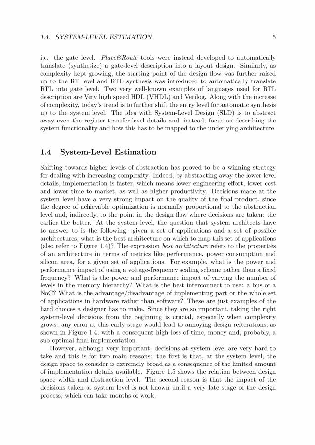
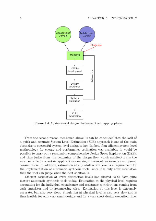
Shifting towards higher levels of abstraction has proved to be a winning strategyfor dealing with increasing complexity. Indeed, by abstracting away the lower-leveldetails, implementation is faster, which means lower engineering effort, lower costand lower time to market, as well as higher productivity. Decisions made at thesystem level have a very strong impact on the quality of the final product, sincethe degree of achievable optimization is normally proportional to the abstractionlevel and, indirectly, to the point in the design flow where decisions are taken: theearlier the better. At the system level, the question that system architects haveto answer to is the following: given a set of applications and a set of possiblearchitectures, what is the best architecture on which to map this set of applications(also refer to Figure 1.4)? The expression best architecture refers to the propertiesof an architecture in terms of metrics like performance, power consumption andsilicon area, for a given set of applications. For example, what is the power andperformance impact of using a voltage-frequency scaling scheme rather than a fixedfrequency? What is the power and performance impact of varying the number oflevels in the memory hierarchy? What is the best interconnect to use: a bus or aNoC? What is the advantage/disadvantage of implementing part or the whole setof applications in hardware rather than software? These are just examples of thehard choices a designer has to make. Since they are so important, taking the rightsystem-level decisions from the beginning is crucial, especially when complexitygrows: any error at this early stage would lead to annoying design reiterations, asshown in Figure 1.4, with a consequent high loss of time, money and, probably, asub-optimal final implementation.
However, although very important, decisions at system level are very hard totake and this is for two main reasons: the first is that, at the system level, thedesign space to consider is extremely broad as a consequence of the limited amountof implementation details available. Figure 1.5 shows the relation between designspace width and abstraction level. The second reason is that the impact of thedecisions taken at system level is not known until a very late stage of the designprocess, which can take months of work.
6 CHAPTER 1. INTRODUCTION
ApplicationsDomain
ArchitecturesDomain
HW/SWdevelopment
Systemprototype
Systemvalidation
Mapping?
Chipfabrication
Reiteration
Challenge
Figure 1.4: System-level design challenge: the mapping phase
From the second reason mentioned above, it can be concluded that the lack ofa quick and accurate System-Level Estimation (SLE) approach is one of the mainobstacles to successful system-level design today. In fact, if an efficient system-levelmethodology for energy and performance estimation was available, it would bepossible to carry out a reasonably comprehensive Design Space Exploration (DSE),and thus judge from the beginning of the design flow which architecture is themost suitable for a certain applications domain, in terms of performance and powerconsumption. In addition, estimation at any abstraction level is a requirement forthe implementation of automatic synthesis tools, since it is only after estimationthat the tool can judge what the best solution is.
Efficient estimation at lower abstraction levels has allowed us to have quitemature automatic synthesis tools today. Estimation at the physical level requiresaccounting for the individual capacitance and resistance contributions coming fromeach transistor and interconnecting wire. Estimation at this level is extremelyaccurate, but also very slow. Simulation at physical level is also very slow and isthus feasible for only very small designs and for a very short design execution time.

1.4. SYSTEM-LEVEL ESTIMATION 7
Design space width
Abst
ract
ion level
Physicallevel
Gate level
RTL levelSystem
level
Figure 1.5: Design space width versus abstraction level
At the gate level, estimation is simplified by the fact that standard cells are used,whose physical properties are pre-characterized. Only the impact of cell-to-cellconnecting wires has to be estimated separately, which is done using so called wireload models. Estimation at this level is less accurate, although faster, and biggerdesign sizes can be simulated. At the RT level, Hardware Description Language(HDL) languages are used to describe in words what RTL synthesis translates intologic gates. Simulation is very common at RT level and reasonably fast for medium-size designs running very short chunks of application. However, estimation madeat this level loses accuracy due to the lack of enough physical details. In general,the increase of the abstraction level is directly proportional to an increase of theestimation speed and inversely proportional to the estimation accuracy.
When it comes to system level, the lack of an efficient estimation methodol-ogy has been an obstacle to having mature automatic system-level synthesis toolsavailable today. In fact, the operation of mapping the system-level functional de-scription to the actual architecture is still largely done manually. The decisionmaking approach used by system designers has been mostly relying on their ac-quired experience, on the comparison with previous designs and on rules of thumb.However, while this approach can still work with small/medium-size systems, itsapplication to today’s more and more complex systems has become unrealistic andthe need for a more systematic and accurate approach has become a necessity. TLMhas appeared at the beginning of the last decade as a simulation-based approachraising the abstraction level above RTL and as a starting point for synthesis. Inessence, TLM abstracts away the RTL details and models functionality and com-munication among the system modules. Communication is seen as an exchangeof transactions between architectural resources. As a result, TLM has proved tobe much faster than RTL [26]. In spite of that, even TLM could be too slow toallow proper simulation of future complex systems. More details about the TLMmethodology are given in Chapter 2. In addition, the problem remains of how toobtain for example accurate power estimation at the system level, since TLM does
8 CHAPTER 1. INTRODUCTION
not provide intrinsic support for power estimation, and waiting until reaching thegate-level design phase is not an option. The natural question that comes as aconclusion of the above discussion and that is thus also the motivation behind thisthesis work is as follows:
As it has been discussed that system-level estimation is essential for a successfulsystem-level design, how is it possible to implement a fast and accurate methodologyfor efficient system-level estimation?
Answering this question is instead the contribution of this thesis.
1.5 Thesis Contribution
The present work contributes to the area of system-level estimation by proposinga system-level estimation framework for energy and performance prediction, whichcan indeed help system designers take the best architectural decisions early in thedesign flow.
The approach consists of three layers. The bottom layer is called IP Level (LevelA) and relies on building a library of IP energy and performance models, whereindividual IP functionalities are pre-characterized in terms of number of cyclesand energy consumption. This activity is justified by the fact that, as discussedbefore, the Design&Reuse concept has become a common industrial practice, andthe modeling process is therefore only a one-time effort. Such models can come inthe form of look-up tables or mathematical expressions. Characterization is doneat the gate level and back-annotated with physical design data to enable highlyaccurate characterization. The availability of a physical layout for each IP alsoallows preliminary floorplans to be made for different architectures. This in turnenables us to get reasonably good estimates of the global wires length, which alsoplays a critical role in affecting the overall system energy and performance. Notethat the characterization activity performed at this level is the prerogative of the IPprovider and not of the system designer, who is the tool end user. As an example,Chapter 4 describes the implementation of an energy and performance model fora SPARC-based Leon3 processor. The impact that the external communicationinfrastructure – connecting IPs to each other – has on the individual IP propertiesis also taken into account. Chapter 5 discusses the case of switching from a bus-based to a NoC-based architecture.
The intermediate layer is called Algorithmic Level (Level B) and is where theactual estimation takes place. As opposed to the IP Level, this level directly con-cerns the system designer. At this level, applications are run and profiled on adevelopment host (a common PC). This allows us to create a trace of the executedsource code, which is then mapped to the assembly code of the target architec-ture. This operation allows a trace of target instructions to be indirectly builtwithout having to run the applications natively on the target architecture. Thishas a few clear advantages: first, the engineering effort is kept low, since there isno need of implementing a high-level simulation model of the target architecture,
1.5. THESIS CONTRIBUTION 9
for instance a transaction-level model. Second, the level of abstraction at whichthe approach proposed in this thesis performs estimation is the functional untimedlevel – from here the whole approach has been called Funtime – which is higherthan the transaction level. As a consequence, estimation is faster. Once the targettrace is inferred, energy and performance figures can be extracted by using the IPmodels from the bottom layer. To make the whole process possible, changes havebeen made to the GNU GCC compiler. Estimation examples are shown for a setof common image/video codec applications in Chapter 6.
The top layer is called Refinement Level (Level C) and accounts for non-idealitiesneglected at the layer below, such as the presence of caches and the fact thatmultiple applications normally run concurrently, share the same resources and arecontrolled by an operating system. Statistical models are built to predict the energyand performance impact of each of these components through extensive simulation.However, this is a one-time activity. When estimation is carried out, these statisticalmodels are used and no simulation is run at all. An MPSoC hosting up to 15processors and using both fixed-priority and round robin bus arbitration is usedfor modeling bus contention. This is part of Chapter 7. The RTEMS operatingsystem is taken as a reference to model the OS energy and performance impact. OSmodeling has considered both the round robin and fixed-priority scheduling cases.This is part of Chapter 8.
Validation for each layer is also carried out. The results show that the approachis within 15% of gate-level accuracy and exhibits an average speed-up of ∼30Xwhen compared to transaction-level modeling (TLM).
Note that the use-case size and the amount of factors that have to be takeninto account when doing system-level estimation are extremely large. Since it wasnot possible to deal with all these aspects within this work, the Funtime frameworkpresented in this thesis comes as a proof of concept. Smaller use-cases have beenused as case studies and sensible simplifications have been made, the goal being toshow the overall feasibility of the Funtime approach as a system-estimation tool.Further extensions are required to make this framework more general and complete,as is discussed in the future work section, at the end of the thesis.
The contribution of this thesis can also be classified into three components:
• Concept-related: this component concerns the definition of the Funtime esti-mation framework and the actual implementation of each of its layers. Start-ing from an initial abstract idea, each layer has in time been shaped andenriched with increasing details.
• Tool-related: each of the three layers has required consistent scripting work,aimed at speeding up and automating operations that could not have beencarried out manually. For instance, at the IP Level, scripts have been writtento automate the Leon3 processor characterization. At the Algorithmic Level,scripts have been written to profile the application running on the develop-ment host and to map it to the target. This activity has also implied a set of

10 CHAPTER 1. INTRODUCTION
changes to the GNU GCC compiler. Finally, at the Refinement Level, scriptshave been written to automate the OS characterization process. Configuringthe RTEMS OS has also required quite some effort, including writing basicdriver routines.
• Experiment-related: experiments have been conducted throughout the entiredevelopment of the Funtime methodology to validate both its estimation ac-curacy and speed. At the IP Level, the accuracy of the Leon3 energy andperformance model has been validated against gate-level measurements for aset of common applications. At the algorithmic level, the same applicationshave been used to test the accuracy of Funtime in inferring a trace of targettransactions and in estimating its energy consumption. At the RefinementLevel, experiments have been conducted to verify the accuracy of Funtime ininferring the OS overhead, the bus contention overhead, as well as the effectof caches. A transaction-level model has been also used to validate Funtime’sestimation speed. The target architectures used as a reference for the exper-iments are a shared-bus MPSoC based on the AMBA AHB bus, and a NoCusing deflective routing algorithm. Leon3 has been taken as the referenceprocessor.
The following publications have been used as a basis for the present thesis:
• Paper [61] gives first an overview of the three layers of the Funtime approachand then presents in more detail the bottom and intermediate layers. Thework presented in this paper has been largely conducted by the author of thethesis, who has defined the details of the Funtime layers and has producedpart of the numerical results. Luca Bolognino was a master’s student whohelped produce the remaining part of the numerical results. Ahmed Hemanicontributed by giving feedback and by conceptually discussing with the thesisauthor the role played by each of the Funtime layers.
• Paper [53] proposes an instruction-level characterization of the Sparc-basedLeon3 processor. The resulting model, in the form of look-up tables, reportsnumber of cycles and energy for each processor instruction. The steps of thecharacterization methodology proposed in the paper have been decided bythe author of this thesis. Luca Bolognino was a master’s student who helpedthe author by doing the tool-related work, according to the guidelines givenby the thesis author. Ahmed Hemani has supported the author with usefulfeedback.
• Papers [58] and [57] investigate the operating system overhead in terms ofenergy and performance. Characterization is first carried out by executingextensive simulation and energy extraction at the gate level. The resultsfrom characterization are then used to implement a high-level model for rapidand accurate OS overhead prediction. Paper [58] considers Round Robinscheduling, while paper [57] considers priority-driven scheduling. The work

1.6. THESIS LAYOUT 11
presented in these papers has been conducted by the author of this thesis andsupported by feedback from Ahmed Hemani and Ingo Sander.
• Paper [59] investigates the effects of bus contention on energy and perfor-mance in MPSoCs. Characterization is first carried out by executing exten-sive simulation and energy extraction at the gate level. The results fromcharacterization are then used to implement a high-level model for rapid andaccurate prediction of bus contention. The work presented in this paper hasbeen conducted by the author of this thesis and supported by feedback fromAhmed Hemani and Ingo Sander.
The following publications, although not used as a basis for this thesis, arereported for the sake of completeness:
• Paper [54] is an initial concept paper which gives a general idea of the Funtimeapproach and its layers. The author of this thesis and Ahmed Hemani haveequally contributed to this work.
• Paper [56] implements an energy and performance model for a switch of theNostrum NoC. The model reports the switch energy per clock cycle, basedon the variation of the switch inputs. The entire work has been conducted bythe author of the thesis and supported by the feedback from Axel Jantsch.
• Paper [55] presents an initial work on the Algorithmic Level, where a set ofapplications is used to validate the accuracy of Funtime in inferring a targetexecution trace. No energy estimation results are presented in this paper,however. The work presented in this paper has been mainly conducted bythe author of this thesis. Mohammad Badawi was a master’s student whohelped with the experimental part. Ahmed Hemani has contributed withuseful feedback.
• Paper [60] extends the paper in [55] by also validating Funtime estimationspeed against a TLM implementation. The work presented in this paper hasbeen mainly conducted by the author of this thesis. Mohammad Badawihas helped with the implementation of the transaction-level model. AhmedHemani has contributed with useful feedback.
• Journal paper [62] is an invited work, as a follow-up of the VLSI 2009 con-ference. It merges and partially extends the contents of the papers in [61]and [53]. The journal paper has been written by the author of this thesis.
1.6 Thesis Layout
Chapter 2 presents an overview of the most common approaches to system-leveldesign/estimation in use today and compares them to the Funtime approach. Largespace is given to the description of simulation-based approaches to system-level
12 CHAPTER 1. INTRODUCTION
design/estimation, with particular focus on Transaction Level Modeling (TLM).The reason is that TLM is a very common approach. Examples of TLM usage inreal projects are then proposed, which also include modeling of Multi-ProcessorSoC (MPSoC)s and Operating System (OS). A minor section is left for discussinganalytical approaches and combinations of multiple approaches.
Chapter 3 presents an overview of the whole Funtime approach. After describingthe methodology user interface, a description follows of the purpose of each of thethree layers of which Funtime consists. In particular, taking a bottom-up approach,an IP Level (Level A), an Algorithmic Level (Level B) and a Refinement Level(Level C) are identified. Afterward, the chapter continues by covering miscellaneousaspects relative to Funtime, with the purpose of providing a more complete andconsistent picture of the approach.
Chapter 4 and 5 go into the details of the IP Level. Chapter 4 shows how to buildan energy and performance model for a processor IP, namely for a Leon3. Chapter 5shows instead how to account for the effects of IP-to-IP external communicationwhen building IP models. A bus-based SoC and a NoC-based SoC are compared.
Chapter 6 gives further details about the Algorithmic Level. This chapter showsexamples of energy and performance estimation on common applications. It alsoshows the accuracy and speedup obtained by Funtime against gate-level extrac-tion and TLM respectively. Due to its tight binding with the Algorithmic Level,this chapter also includes two refinements from the Refinement Level, concerningtransactions interdependency and the effects of caches.
Chapter 7 and 8 present extensively two other refinements. In particular, Chap-ter 7 proposes a high-level method to predict bus contention in MPSoCs, whileChapter 8 presents a high-level method to predict the overhead of OS.
Chapter 9 draws the conclusions on the entire work and leaves space for somefuture work.

Chapter 2
Common Approaches toSystem-Level Estimation andDesign Today
This chapter presents a survey of the most important methodologies for system-level estimation and design found in the literature, and compares them to Funtime.Three categories of tools are identified: simulation-based tools, analytical tools andtools that are a combination of multiple approaches. While discussing each of thesecategories, larger space is dedicated to simulation-based tools and, in particular, todescribing SystemC/TLM. The reason is that Transaction-Level Modeling has be-come quite popular today, both in industry and academia, and is taken as a referencemethodology to which Funtime is compared throughout this thesis.
2.1 Introduction
In the previous chapter, the conclusion was drawn that being able to efficientlycarry out system-level estimation (SLE) is a prerequisite to making design-spaceexploration (DSE) at system level possible. In turn, DSE is critical to enable asuccessful system-level design (SLD), since it both helps system designers take thebest architectural decisions and it is also an essential component for system-levelsynthesis.
Due to their importance and to the lack of a standard approach, both system-level estimation and system-level design in general are a hot research topic todayand the focus of a high number of research groups. The present chapter presents asurvey of the most significant estimation tools for SLD/SLE found in the literature.In doing so, the surveys presented in [79] and [28] are partially taken as a referenceand adapted to the purposes of this work. At the same time, a comparison ispresented between these approaches and Funtime, which emphasizes key similaritiesand differences.
13

14CHAPTER 2. COMMON APPROACHES TO SYSTEM-LEVEL ESTIMATION
AND DESIGN TODAY
System-level estimation tools can roughly be classified into three broad cate-gories: simulation-based tools, analytical tools, and tools that are a combinationof different approaches. Although the following subsections review each category,large space is dedicated to the simulation-based approaches and, in particular, todescribing SystemC and Transaction Level Modeling (TLM). The reason is that thissimulation-based approach has lately gained consensus and has become quite pop-ular in both the industrial and academic community. This is why SystemC/TLMis also used in this work as the reference system-level approach when validatingFuntime for estimation speed.
2.2 Simulation-Based Estimation Tools
As the name suggests, these tools rely on simulation to produce estimation results.Simulation allows us to trace the behavior of the system in specific states and givena certain set of input stimuli. Simulation-based approaches are therefore suitablefor non-deterministic system behavior and their results are generally representativeof the average-case scenario. Simulation-based approaches have two drawbacks:one is the large engineering effort required to develop a model of the system – thearchitectural model – and the second is that the simulation of an application modelin such an architectural model is very slow and for large and complex use casesthe simulation time can be unreasonably large. Below, a few simulation-based ap-proaches are presented.
Ptolemy [19] is a framework capable of modeling and simulating concurrentand hierarchical heterogeneous systems. Hierarchy is supported in that the wholesystem model can consist of a tree of nested sub-models. At each level of hierarchy,such sub-models are composed to form a network of interacting components. Eachlocal network is constrained to be homogeneous, whereas heterogeneity is allowedbetween networks at different levels of hierarchy. The interaction mechanism withina certain local network of components handles both data and control flow among thelocal components. Such an interaction mechanism is called model of computation(MoC). Note that, since different MoCs are allowed at different levels of hierarchy,different parts of the system can be modeled at different levels of abstraction,depending on the required degree of detail.
More concretely, Ptolemy relies on an actor-oriented view of a system, whereactors are concurrent components communicating with each other by using com-munication channels connected to the actor’s ports. Every actor can either run inits own thread or multiple actors can run sequentially in a unique thread. Thisis determined by the local MoC. An actor is called atomic if it is at the bottomof the hierarchy, while it is called composite when it contains other actors. Theimplementation of a MoC related to a composite actor is called domain. A domaindefines both the communication semantics and the order of execution among thelocal actors. In detail, communication is controlled by receivers, which are located

2.2. SIMULATION-BASED ESTIMATION TOOLS 15
at each actor input port and are unique for each channel. Receivers can representFIFOs, mailboxes, proxies for a global queue or rendezvous points. The executionorder of the local actors is instead controlled by a director.
Figure 2.1 shows a hierarchical example with two domains which are, by defini-tion, associated with two composite actors. The top-level actor contains a directorD1, an atomic actor A1 and a composite actor A2, which contains a director D2and the atomic actors A3 and A4. D1 controls the execution order of A1 and A2,while D2 the execution order of A3 and A4.
Figure 2.1: Ptolemy hierarchical model using two different domains. Source: [19].
SpecC [24], [13] is both a system-level design language and methodology inwhich computation is separated from communication. Computation happens insideso called behaviors, while communication is implemented by channels. Channels areconnected to behaviors through behaviors’ ports, as long as the respective interfacesmatch. Hierarchy is also supported, in that both behaviors and channels can residewithin a parent behavior. Execution occurs within each behavior and synchroniza-tion among behaviors is implemented by events. An example of a SpecC design isshown in Figure 2.2.
SpecC is based on the C language, which is extended with hardware and soft-ware modeling constructs. As will be evident in the next few subsections, SpecCis in many respect similar to SystemC, as this also allows a separation betweencomputation and communication. However, SystemC is an extension of C++.
Metropolis [8] provides a tool-set targeting embedded systems development,which supports simulation, formal analysis and synthesis. The authors state thatusing a unified framework, rather than a collection of unlinked tools, as is the casetoday, can considerably speed up the entire design flow, by making it more efficientand less error prone.
The Metropolis infrastructure relies on a so called metamodel, which is a modelwith precise semantics and general enough to support both existing and new mod-els of computation. In this respect, Metropolis includes a standard API, whichallows feeding the tool with inputs coming from any external tool. The Metropolismetamodel is a language, similar to SystemC, that specifies networks of concurrentobjects. This metamodel can be used to represent function, architecture, mapping
16CHAPTER 2. COMMON APPROACHES TO SYSTEM-LEVEL ESTIMATION
AND DESIGN TODAY
Figure 2.2: SpecC design methodology. Source: [18].
of the function on the architecture, and platforms.A function is seen as a set of objects – called processes – that concurrently carry
out some actions while communicating with each other through ports. Ports comewith interfaces, which declare a set of methods usable by the process through theport. The interface methods are actually implemented in other objects calledmedia,which are used to connect ports to each other. Channels are the SystemC equivalentof Metropolis media. The behavior of this network of processes is modeled as a set ofexecutions, where each execution consists of a sequence of events. Events representa program’s entries or exits to some piece of code. Note that Metropolis is inmany respects similar to Ptolemy, SpecC and SystemC, in that they all rely on theconcept of concurrent processes that communicate via channels.
An architecture is identified in Metropolis by two aspects: the functionality thatit has to implement and the efficiency of such implementation. As was discussedabove that functionality is basically the expression of some services implementedby methods, efficiency is measured by accounting for the cost of such services. Thisis done by annotating the cost of each atomic event executed within a process.So called quantity managers are used for this purpose. The decomposition of ser-vices into event sequences is done by using networks of media and processes, as isalso done for the functional model. Architecture networks often match the actualphysical structure of the architecture.
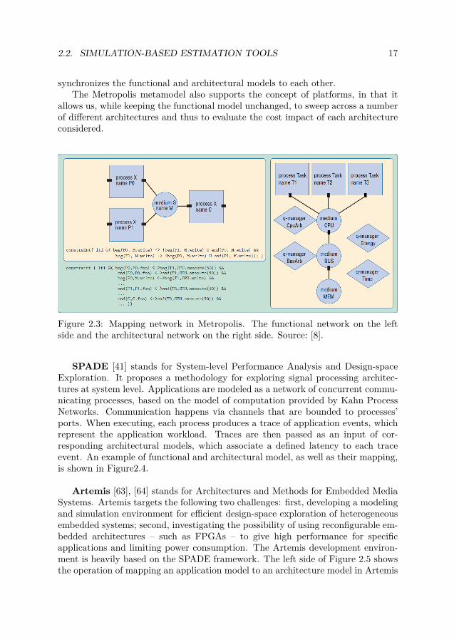
The Metropolis metamodel also takes care of mapping the functional model tothe architectural model. This is done by using a new network – called MappingNetwork – that contains the functional and architectural networks and synchronizesone to the other by means of events. Figure 2.3 shows an example of a functionalmodel on the left side and of a corresponding architectural model on the rightside. Note the presence of quantity managers in the architectural model. Thetext with green background describes instead the mapping networks that maps and
2.2. SIMULATION-BASED ESTIMATION TOOLS 17
synchronizes the functional and architectural models to each other.The Metropolis metamodel also supports the concept of platforms, in that it
allows us, while keeping the functional model unchanged, to sweep across a numberof different architectures and thus to evaluate the cost impact of each architectureconsidered.
Figure 2.3: Mapping network in Metropolis. The functional network on the leftside and the architectural network on the right side. Source: [8].
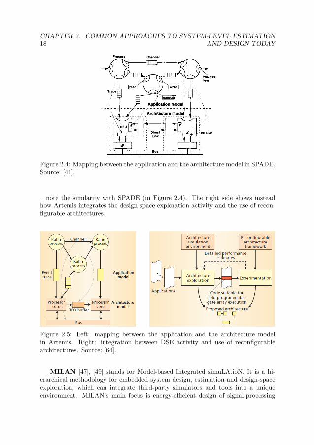
SPADE [41] stands for System-level Performance Analysis and Design-spaceExploration. It proposes a methodology for exploring signal processing architec-tures at system level. Applications are modeled as a network of concurrent commu-nicating processes, based on the model of computation provided by Kahn ProcessNetworks. Communication happens via channels that are bounded to processes’ports. When executing, each process produces a trace of application events, whichrepresent the application workload. Traces are then passed as an input of cor-responding architectural models, which associate a defined latency to each traceevent. An example of functional and architectural model, as well as their mapping,is shown in Figure2.4.
Artemis [63], [64] stands for Architectures and Methods for Embedded MediaSystems. Artemis targets the following two challenges: first, developing a modelingand simulation environment for efficient design-space exploration of heterogeneousembedded systems; second, investigating the possibility of using reconfigurable em-bedded architectures – such as FPGAs – to give high performance for specificapplications and limiting power consumption. The Artemis development environ-ment is heavily based on the SPADE framework. The left side of Figure 2.5 showsthe operation of mapping an application model to an architecture model in Artemis
18CHAPTER 2. COMMON APPROACHES TO SYSTEM-LEVEL ESTIMATION
AND DESIGN TODAY
Figure 2.4: Mapping between the application and the architecture model in SPADE.Source: [41].
– note the similarity with SPADE (in Figure 2.4). The right side shows insteadhow Artemis integrates the design-space exploration activity and the use of recon-figurable architectures.
Figure 2.5: Left: mapping between the application and the architecture modelin Artemis. Right: integration between DSE activity and use of reconfigurablearchitectures. Source: [64].
MILAN [47], [49] stands for Model-based Integrated simuLAtioN. It is a hi-erarchical methodology for embedded system design, estimation and design-spaceexploration, which can integrate third-party simulators and tools into a uniqueenvironment. MILAN’s main focus is energy-efficient design of signal-processing

2.2. SIMULATION-BASED ESTIMATION TOOLS 19
applications. The following steps are identified in this framework flow: applicationmodels are first created using synchronous data flow (SDF) graphs. MILAN sup-ports hierarchical modeling of SDF graphs. Functional simulation is enabled bythe generation of high-level source code in C or Matlab and by the integration offunctional simulators. Second, a model for the architectural resources is created,on which the user defines a set of performance constraints, in terms of latencyand energy. Once these steps are completed, the user invokes the DSE tools. Thepredefined DSE tool in MILAN is called DESERT. This tool relies on Ordered Bi-nary Decision Diagrams for constraint satisfaction. The authors also report thatDESERT is able to cover a design space of around 1020 ∼ 1040 designs in a fewminutes. The output of DESERT is then passed to and evaluated by the High-levelPerformance Estimator (HiPerE) tool. This tool estimates system-level energy dis-sipation and latency. Estimation is carried out at the task level abstraction, whichconfers the tool high speed. Both this tool and the actual architectural model arebased on a so called General Model (GenM) [48]. The designs selected by HiPerEare then passed to lower-level simulator/estimator for the final design selection.Figure 2.6 shows the complete MILAN flow. From left to right, it is possible toidentify the user’s application and architectural resources model, together with theconstraints definition; the usage of DESERT and of HiPerE is also shown.
Figure 2.6: MILAN design, DSE and estimation framework. Source: [49].
TAPES [76] stands for Trace-based Architecture Performance Evaluation withSystemC. In order to keep simulation as fast as possible, the functionality of eachresource is modeled as a sequence of processing delays interleaved with externaltransactions, and resources are considered as black boxes. Such a sequence is calleda trace. External transactions are typically read/write transactions used to model

20CHAPTER 2. COMMON APPROACHES TO SYSTEM-LEVEL ESTIMATION
AND DESIGN TODAY
communication which, as opposed to functionality, is not modeled with the samedegree of abstraction. A more detailed model for communication is considerednecessary in order to properly account for the occurrence of contention events. Atthe communication level, the read/write transactions emitted by functional modelsare thus expanded to account for the actual communication behavior. An exampleis shown in Figure 2.7: the trace on the top reflects the functionality of a CPU,which emits two consecutive read transactions, executes some internal functionalitymodeled by a delay, and finally emits a write and read transaction. The trace atthe bottom shows instead how the CPU trace is transformed during architecturalsimulation, to account for the bus and memory accesses.
Figure 2.7: TAPES trace example. Source: [76].
TAPES is not only an estimation tool, but also a framework in which to carryout architectural exploration. Besides high simulation speed, this also implies thatfast changes of the system architecture must be made possible. For this purpose,the hardware configuration of the simulation model is dynamically changed at thebeginning of the simulation according to a system configuration file. This meansthat users do not have to manually modify the SystemC description. Note that thetrace specification for the system architecture is instead a manual process, and thetiming behavior of the resources is taken either from data sheets or, for the CPU,by using an instruction-set simulator.
MESH [52], [46] stands for Modeling Environment for Software and Hardware.It is defined by the authors as a thread-level simulator, as opposed to traditionalinstruction-set simulators. In this way, the authors want to emphasize that MESHincreases the granularity for which estimation is carried out and thus the simula-tion speed can be much higher. MESH is a three-layer approach, which considersresources (hardware blocks), software and schedulers. Such layers are modeled bysoftware threads on the evaluation host. Software threads are annotated with timebudgets for the corresponding hardware elements. Such time budgets are extractedbeforehand by estimation or profiling. Scheduler threads work as arbiters for thesoftware threads. Power estimation capabilities are also implemented in MESH. As

2.2. SIMULATION-BASED ESTIMATION TOOLS 21
far as microprocessors are concerned, the authors rely on the fact that compilerstend to produce quite regular instructions patterns, from which a power estimatecan be extracted, that is representative of the average case.
As part of the ASSET project, Joshi et al. [34] propose a performance evalu-ation methodology for system-level design exploration. The application behavioris modeled as a set of statistical parameters, which are generated either by staticanalysis and profiling of the application, or by using some simulation frameworklike SimpleScalar [7]. Application parameters are independent of the architectureand their extraction is a one-time activity. The target architecture componentsare instead modeled using SystemC. A set of components on which to map theapplication models is taken from a library. Building these components also relieson probabilistic models, which are extracted by making a compromise between an-alytical and cycle-accurate simulation, and which only account for the interactionthe component has with the outside, while the internal functionality is modeled asa delay. Note that, during the mapping phase, application parameters must alsomatch with the parameters of the component the application is mapped to. Forexample, an application parameter could be the distribution of load instructions,whereas the corresponding architectural parameter could be the number of wordsto be loaded.
J. Kreku et al. in [35] also present a methodology for system-level design andperformance evaluation. Their work relies on describing application workloads inUML and platform services in SystemC. The methodology is meant to enable earlysystem-level performance modeling and evaluation through transaction-level simu-lation, which also allows timing information to be collected.
Simulators have also been developed to investigate the properties of some pro-cessor micro-architectures. Such simulators are often cycle-accurate. Some exam-ples are SimpleScalar [7] or SimOS [65]. Simics [42] is instead a virtualizationframework that allows entire platforms to be emulated.
2.2.1 An overview of SystemC and Transaction LevelModeling (TLM)
Among the simulation-based approaches, those relying on SystemC/TLM or anequivalent modeling style deserve a dedicated section. The reason is that, in recentyears, SystemC/TLM has become quite popular and has found a relatively widerange of applications both in academia and industry. SystemC’s popularity is inpart also the result of backing by leading industrial players like Coware (now partof Synopsys), Synopsys and Cadence.
SystemC is both an HDL and a High-Level Language (HLL) [30]. In fact, itmodels hardware at a higher abstraction level than Register Transfer Level (RTL)and, in order to do this, it uses C++ as a programming language. Higher ab-straction level means higher simulation speed but also less accuracy. The way Sys-temC/TLM trades-off these two important metrics has been characterized in [67].
22CHAPTER 2. COMMON APPROACHES TO SYSTEM-LEVEL ESTIMATION
AND DESIGN TODAY
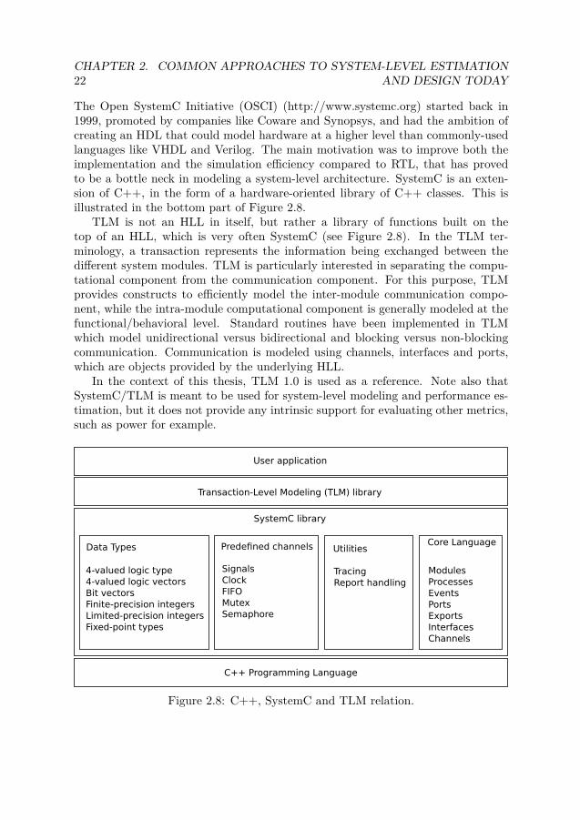
The Open SystemC Initiative (OSCI) (http://www.systemc.org) started back in1999, promoted by companies like Coware and Synopsys, and had the ambition ofcreating an HDL that could model hardware at a higher level than commonly-usedlanguages like VHDL and Verilog. The main motivation was to improve both theimplementation and the simulation efficiency compared to RTL, that has provedto be a bottle neck in modeling a system-level architecture. SystemC is an exten-sion of C++, in the form of a hardware-oriented library of C++ classes. This isillustrated in the bottom part of Figure 2.8.
TLM is not an HLL in itself, but rather a library of functions built on thetop of an HLL, which is very often SystemC (see Figure 2.8). In the TLM ter-minology, a transaction represents the information being exchanged between thedifferent system modules. TLM is particularly interested in separating the compu-tational component from the communication component. For this purpose, TLMprovides constructs to efficiently model the inter-module communication compo-nent, while the intra-module computational component is generally modeled at thefunctional/behavioral level. Standard routines have been implemented in TLMwhich model unidirectional versus bidirectional and blocking versus non-blockingcommunication. Communication is modeled using channels, interfaces and ports,which are objects provided by the underlying HLL.
In the context of this thesis, TLM 1.0 is used as a reference. Note also thatSystemC/TLM is meant to be used for system-level modeling and performance es-timation, but it does not provide any intrinsic support for evaluating other metrics,such as power for example.
C++ Programming Language
Data Types
4-valued logic type4-valued logic vectorsBit vectorsFinite-precision integersLimited-precision integersFixed-point types
ModulesProcessesEventsPortsExportsInterfacesChannels
Predefined channels
SignalsClockFIFOMutexSemaphore
Utilities
TracingReport handling
Transaction-Level Modeling (TLM) library
User application
SystemC library
Core Language
Figure 2.8: C++, SystemC and TLM relation.
2.2. SIMULATION-BASED ESTIMATION TOOLS 23
2.2.2 Time representation in TLM
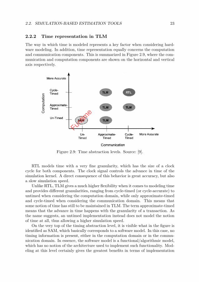
The way in which time is modeled represents a key factor when considering hard-ware modeling. In addition, time representation equally concerns the computationand communication components. This is summarized in Figure 2.9, where the com-munication and computation components are shown on the horizontal and verticalaxis respectively.
Computation
Figure 2.9: Time abstraction levels. Source: [9].
RTL models time with a very fine granularity, which has the size of a clockcycle for both components. The clock signal controls the advance in time of thesimulation kernel. A direct consequence of this behavior is great accuracy, but alsoa slow simulation speed.
Unlike RTL, TLM gives a much higher flexibility when it comes to modeling timeand provides different granularities, ranging from cycle-timed (or cycle-accurate) tountimed when considering the computation domain, while only approximate-timedand cycle-timed when considering the communication domain. This means thatsome notion of time has still to be maintained in TLM. The term approximate-timedmeans that the advance in time happens with the granularity of a transaction. Asthe name suggests, an untimed implementation instead does not model the notionof time at all, thus allowing a higher simulation speed.
On the very top of the timing abstraction level, it is visible what in the figure isidentified as SAM, which basically corresponds to a software model. In this case, notiming information is present, either in the computation domain or in the commu-nication domain. In essence, the software model is a functional/algorithmic model,which has no notion of the architecture used to implement such functionality. Mod-eling at this level certainly gives the greatest benefits in terms of implementation

24CHAPTER 2. COMMON APPROACHES TO SYSTEM-LEVEL ESTIMATION
AND DESIGN TODAY
and simulation speed, but at the same time introduces the biggest challenges topreserving estimation accuracy. It is at this level that the estimation approach pro-posed in this work, i.e. Funtime, operates. In the upcoming chapters, challenges,advantages and drawbacks of this choice are discussed.
2.2.3 TLM advantagesBased on what has been said so far, using TLM has some clear benefits:
1. Compared to a traditional RTL approach, TLM allows a higher implemen-tation speed. Implementation speed comes from the fact that all the RTLdetails are abstracted away. In practice, this means that the actual imple-mentation details of the computational blocks are omitted and replaced by afunctional/behavioral description. Behavioral description is faster to imple-ment than architectural description. In [26], the author reports a speedup ofup to 10X when modeling in TLM compared to RTL.
2. Compared to a traditional RTL approach, TLM also enables a higher simula-tion speed, which in [26] is estimated to be up to 1000X higher than RTL. Thisresult is mainly related to the time representation in TLM. From what wasdiscussed above, an untimed implementation in the computational domaincombined with an approximate-timed implementation in the communicationdomain give the best TLM simulation performance.
3. F. Ghenassia in [26] states that using the TLM design flow can allow a moreefficient HW/SW co-design. This is shown in Figure 2.10. In essence, theTLM flow would allow a concurrent development of hardware and software:the architectural TLM of the hardware infrastructure enables early softwaredevelopment and verification of hardware software interfaces. This is also aconsequence of the fact that, in the classic design flow, software is usuallyimplemented in C/C++, while hardware in VHDL/Verilog. In the TLM flowinstead, both the software and hardware models are implemented in C/C++;thus concurrent testing becomes more feasible and the overall design timeshorter.
4. According to Yi et al. in [78], TLM, and SystemC in general, have helpedto solve some annoying synchronization issues. This aspect is mainly relatedto the fact that, in a simulation-based approach, multiple simulation modelsmay have to run together and synchronize to each other. The introductionof SystemC has contributed to reducing the severity of this problem by pro-viding a homogeneous environment for hardware/software co-simulation, thusreplacing the considerable Inter-Process Communication (IPC) overhead witha light-weighted thread switch overhead. However, Yi et al. state that “formore accurate cosimulation, ISSs are typically used in SystemC cosimulation[...]. ISSs are attached to a cycle accurate transaction level communication ar-chitecture model and communicate via IPC.”. Handling and reducing the IPC

2.2. SIMULATION-BASED ESTIMATION TOOLS 25
Figure 2.10: TLM-based design flow. Figure taken from [26].
overhead is therefore an issue that system-level design based on architecturalsimulation still has to cope with. The way Funtime deals with synchroniza-tion and time representation is instead discussed in Section 3.7.
5. Finally, SystemC/TLM is considered the right modeling language from whereHigh-Level Synthesis (HLS) should start. An example to substantiate thisclaim is the CtoS tool sold by Cadence. Starting from a SystemC description,this tool outputs RTL code. In spite of this, HLS is far from being as matureas logic synthesis and therefore requires more research.
2.2.4 TLM drawbacksWhile TLM has many benefits as discussed, it also has some drawbacks. The workproposed in this thesis overcomes these drawbacks.
1. Although the modeling effort happens at a higher abstraction level than RTLand is therefore less time-consuming, TLM is still based on a programminglanguage. This means that the system designer has first to learn how to usethis language – learning SystemC in this case– and then s/he has to implementthe system using this language. Both the learning and implementation processimply a considerable engineering effort and, since the RTL modeling stepcannot yet be replaced by HLS, the TLM step is an extra step in the overallSoC design flow.

26CHAPTER 2. COMMON APPROACHES TO SYSTEM-LEVEL ESTIMATION
AND DESIGN TODAY
2. Although the TLM simulation is more efficient than the RTL time, yet TLMrelies on the availability of a hardware simulation model. Simulation of thetarget system on a host system, which is usually a common x86 PC, is time-consuming and will always introduce a significant overhead compared to na-tive execution. Keeping in mind that the overall HW/SW complexity of SoCsis steadily increasing, even TLM at some point might become too slow to sim-ulate complex and real use-case scenarios.
2.2.5 Examples of SystemC/TLM usage in RTOS and MPSoCsmodeling
In [77], Yi et al. present an approach to Real-Time OS (RTOS) modeling that relieson pre-characterizing the key RTOS components, like the tick interrupt (triggeredby the system timer) and the context switch. The authors rely then on Instruction-Set Simulation (ISS) to run their applications and measure the task duration, inorder to derive the actual number of RTOS occurrences. Once this number is knownand thanks to the pre-characterization activity, the total RTOS impact can thus beestimated. In [78], Yi et al. extend the work done in [77] by using a trace-drivenco-simulation in SystemC. In [11], Brandolese et al. also propose a method to pre-characterize system calls of an OS for embedded applications. To do this, they relyon measurements “based on executing stubs, i.e. suitable programs calling a givenfunction for a large number of times under possibly varying conditions”. However,they only characterize the impact on latency and neglect the impact on energy.
In contrast to [77], [78] and [11], Hessel et al. [32] do not pre-characterize theRTOS, but propose an RTOS model in SystemC, by extending the built-in schedulerthat also does the power estimation. The authors state that “This estimation isbased on previous analysis of the scheduling algorithms. The estimation parameteris update [sic] by back-annotation techniques.”. However it is not very clear whatthis analysis consists of and at what level the back-annotation is done. In [33], theauthors extend the work done in [32] by introducing an abstract RTOS schedulingmodel that “[...] enables the system designer to quickly evaluate different schedulingpolicies and make the best choice in early design stages.”. Partially based on [33],Shaout et al. [69] define and provide the primitives for an ideal API for a genericRTOS model in SystemC.
In a similar fashion, also Le Moigne et al. [40] describe “a generic RTOS modelfor simulation of real-time systems at a high abstraction level with SystemC.”. Intheir implementation, they are particularly concerned with achieving a very accu-rate RTOS time representation, although the RTOS energy impact is ignored. Asan example, when modeling context switches, they distinguish among context loadand save durations and scheduling algorithm duration.
Other research groups have also used the SystemC language as the basis forbuilding their own RTOS models. In [5], an extension of the SystemC simula-tion engine is proposed, where a new simulation library is added to implement theso called T-THREADs, which are Task Thread processes derived from the origi-
2.3. ANALYTICAL ESTIMATION TOOLS 27
nal SystemC SC_THREAD processes. In a similar fashion, in [31] the SystemCSC_THREAD processes are also exploited to create an OS model. The authorsrely on timed OS simulation based on delay annotation, where timing informationis derived from benchmark data provided by the OS vendor.
As for modeling the OS, high-level simulation-based tools are also used formodeling other system-level aspects, such as MPSoCs and bus contention. Many ofthem rely on TLM. In [71] the authors choose an approximately-timed transaction-level implementation to evaluate the timing effects due to bus contention whenmapping applications to MPSoCs. The model is written in SystemC. In [68], theauthors also use TLM to increase communication speed in MPSoC design. However,since they are also interested in speeding up computation, they build abstractprocessor models for fast software simulation. Such processor models, which arebased on SpecC, do not simulate the instruction set architecture; instead, theyabstract it away and only reflect the processor and software behavior. In [66], amethodology is proposed for software estimation in heterogeneous multiprocessorsystems. Applications are represented as a set of tasks forming a fork-join taskgraph, while the architecture is specified using the High-level Machine Description(HMDES) language [16].
2.3 Analytical Estimation Tools
The advantage of analytical methods over simulation-based methods is that theydo not rely on an executable system model and, in general, their estimation speedis much higher than the speed of their simulation-based counterpart. Nonetheless,analytical approaches often take into account the worst-case scenario and thereforethey may be too pessimistic in certain circumstances. For this reason, analyticalmodels are well suited to systems for which it makes sense to assume a deterministicor worst-case behavior, regardless of the input stimuli.
Event stream-based models are an example of an analytical approach. In thiscase, estimation relies on evaluating the task execution on shared resources forevent streams, like periodic events. Network calculus [39] and queuing theory areexamples of how to use event-stream models for making estimation. The former hasbeen applied to network processor design [72], [73], [29] and embedded real-timesystems in general [15]. The latter has been used, among other things, for doingperformance estimation and modeling contention in MPSoCs [6].
2.4 Estimation Tools Based on the Combination ofMultiple Approaches
These tools aim at reducing the total estimation time by running the minimumamount of simulations. From there, all the useful information is collected andreused through analytical considerations to make further estimations.

28CHAPTER 2. COMMON APPROACHES TO SYSTEM-LEVEL ESTIMATION
AND DESIGN TODAY
This approach is common for the evaluation of caches and memory structures.In this case, a single initial simulation generates a trace of all the memory accesses.Since the cache model is known, this trace can then be used to calculate the overallperformance and hit/miss figures. The same trace can be reused for different cachestructures, which allows us to save time otherwise wasted in simulation. Interest-ing work using such trace-driven approach for memory subsystems exploration canbe found in [74], [20], [27]. The same trace-driven technique has also been appliedin [38], [36], [37] to the design of on-chip communication structures: through an ini-tial simulation, a trace recording the inter-module communication history has beengenerated, which has then be used to make estimations on the best communicationconfiguration for the given design.
A variant of this mixed approach consists in going through an initial charac-terization process by running a set of simulations. The information extracted inthis way is collected and given as an input to analytical models for further estima-tion purposes. This technique has been applied to caches performance analysis anddescribed in [21], [22].
In [10], a stochastic bus contention model for MPSoCs is used together withcode execution on the host platform. Estimation relies on the alternation of twophases: a first calibration/characterization phase aims at building and training astochastic model for a sufficiently long time on a cycle-accurate simulation. In asecond phase, the stochastic model is used together with code execution on thehost platform to detect contention. Since this abstraction level is much higher thanthe cycle-accurate level, it allows us to increase the granularity used to model eachsingle advance in time of the target and, consequently, also the estimation speed.The length and the number of times these two phases alternate with each otherduring a use-case estimation is variable. This work has been developed within thecontext of MESH [52].
2.5 Which Category Does Funtime Belong to?
This section compares the key features of Funtime to significant approaches re-viewed so far. This allows us to conclude that Funtime is a combination of simulation-based and stochastic tools.
Funtime as a simulation-based tool. Simulation happens in Funtime duringthe characterization phase, where energy and latency figures are collected from aback-annotated gate-level netlist. This information allows us to create energy andperformance models for IPs (see Chapter 4 and 5), for the OS (see Chapter 8), andit allows us to model bus contention (see Chapter 7) or the effect of caches (seeChapter 6). However none of these are executable models, but just look-up tablesor mathematical expressions. It is emphasized that the characterization phase isa one-time activity to be carried out by the IP or the OS provider and, as such,gate-level simulation is not part of the actual estimation activity and does not

2.5. WHICH CATEGORY DOES FUNTIME BELONG TO? 29
at all concern the system designer using Funtime. In fact, estimation in Funtimedoes not involve simulating the architecture, either at gate level or at a higherabstraction level. Instead, it only involves running and profiling an instrumentedapplication on the development host (a common PC). In this last aspect, Funtimedifferentiates itself from the majority of the simulation-based approaches reviewedin the past sections, especially from those based on SystemC/TLM. In fact, many ofthese approaches carry out estimation through a comprehensive simulation, whichincludes simulating architectures and applications.
As far as OS modeling is concerned, Funtime partially resembles the approachpresented in [77], since this approach also uses simulation only to pre-characterizethe OS, and not during the actual estimation. However, in [77] characterizationis done only to factor in the extra latency induced by RTOS and it ignores theimpact on energy, which is instead considered in this work. Besides, the authorsrely on Instruction-Set Simulation (ISS) to run their applications and measure thetask duration, in order to derive the actual number of clock ticks. In [78], Yi etal. extend the work done in [77] by using a trace-driven co-simulation in SystemC.The Funtime methodology, in contrast to both [77] and [78], does not simulatethe architecture in SystemC or in ISS. As described in detail in the next chapters,estimation in Funtime consists of a first phase where applications run on the de-velopment host and are profiled with target-specific details, and of a second phasewhere the estimation of the OS contribution, as well as of bus contention and cacheeffects, comes in the form of a refinement activity which does not involve simulationat all.
Funtime as a stochastic tool. The energy and performance models resultingfrom the characterization activity are in the form of look-up tables or analyticalexpressions. Funtime uses these models during the estimation activity in orderto back-annotate the applications that, let us recall it, are compiled for, and arerunning on the evaluation host. Because it relies on models that are calibrated onthe average case, Funtime can also be considered as a stochastic tool.
As discussed in Section 2.3, the approach adopted in [10] in the context of theMESH framework [52] also estimates bus contention by using stochastic modelstogether with execution of the application on the host. However, Funtime differsmainly in the following two aspects. First, while the authors in [10] alternate mul-tiple times between the training and the execution phases during the estimation ofa single application, training is done in Funtime only once on a set of significantreference benchmarks used to calibrate the contention model. This avoids intro-ducing extra delays. The calibrated model for contention prediction is then appliedat the end of the code execution. For the details about bus contention predictionin Funtime, please refer to Chapter 7. Second, the approach here proposed alsoaccounts for the bus contention impact on energy consumption. In order to haveaccurate energy figures, the stochastic model is trained on a gate-level netlist.


Chapter 3
An Overview of the FuntimeEstimation Framework
This chapter presents an overview of the Funtime estimation framework. The pre-sentation begins with the Funtime user interface, followed by a detailed introductionto the three layers of the Funtime: the IP Level, the Algorithmic Level and the Re-finement Level. This is followed by miscellaneous aspects related to Funtime, withthe purpose of providing a more complete and consistent picture of the approach.
3.1 Introduction
As mentioned in the previous chapters, the contribution of this work is to proposea fast and accurate energy and performance estimation framework that operatesat the functional untimed (or algorithmic) level of abstraction. Subsection 1.5 andChapter 2 have both summarized the key features of the Funtime approach aswell as compared it to other common approaches, with particular focus on TLM.This chapter describes the Funtime methodology in detail. Figure 3.1 is used as areference throughout the chapter in order to ease the approach description.
Figure 3.1 is vertically split into three columns: the external left column identi-fies the Funtime User Interface, the right column identifies the Funtime output interms of energy and performance prediction, while the central column contains theFuntime core. This is further split horizontally into three layers which, adoptinga bottom-up view, are as follows: the IP Level (Level A), the Algorithmic Level(Level B) and the Refinement Level (Level C). In Figure 3.1, annotations in redpoint to the section/chapter where each level is discussed in detail. In addition,while describing each level from A to C in the next sections, a pedagogical exampleis built up with the purpose of helping the reader to better understand the way themethodology operates in reality.
31

32CHAPTER 3. AN OVERVIEW OF THE FUNTIME ESTIMATION
FRAMEWORK
InstrumentationRunning the instrumented
applications on the evaluation host
A1 - Individual IPs
B - Algorithmic Level
C - Refinement LevelRefinements- Transactions interdependency- Hw/sw optimizations (caches, etc.)- Operating System - Bus arbitration
primarytransactions
primary+
secondary transactions
Output
x
A2 - Architecture of IPs
A -
IP L
evel
:= Database of IP energy and performance models
UCS
AS
UserInterface
:= Database of applications (algorithmic models)
(Sec. 3.3.1 and Ch. 4)
(Sec. 3.3.2 and Ch. 5)
(Sec. 3.4 and Ch. 6)
(Sec. 3.2)
(Sec. 3.5)
(Ch. 7)(Ch. 8)
Energy
Exec. time
(Sec. 6.2)(Sec. 6.4)
exte
nd
ed
IP m
od
els
Figure 3.1: Funtime 3-layer estimation framework
3.2 Funtime User Interface
Funtime expects to receive two pieces of information from the user: an ArchitectureSpecification (AS) and a Use Case Specification (UCS). The AS symbolically tellswhich IPs compose the design, how they are connected to each other and how theyare configured. However, this information does not represent or refer to a hardwaresimulation model, since this would go against the whole idea that Funtime restson: avoiding any high-level simulation of the hardware. The IPs that can be usedin the AS must of course have a corresponding model in the IP models databaseA to allow estimation. This constraint is shown in Figure 3.1 by a dashed arrowbetween the IP models database and the AS.
The UCS instead contains information on how the design described in the ASis meant to be used. Examples can be the following: 1. The applications usedfor the specific test case; 2. The way such applications have been mapped to theresources specified in the AS; 3. The time offset at which each application getstriggered; 4. The input data; 5. The I/O from which the data is received, 6.The I/O through which the data is sent out and 7. OS-related details, such asscheduling policy, clock tick frequency, possible interrupts, etc. As for the AS case,the applications mentioned in the UCS must be present in the applications databaseB. This constraint is shown by a dashed arrow between the applications database

3.3. LEVEL A – THE IP LEVEL 33
and the UCS.The AS and UCS can be also seen in this way: while the AS contains the infor-
mation about the physical connection of the IPs, the UCS contains the informationabout the logic one.
As of today, both the AS and UCS information are fixed in an ad hoc manner,while a more formal representation, for example in the form of a file, is part of thefuture work.
3.3 Level A – The IP Level
The IP Level is concerned with characterizing the Intellectual Properties as SoCbuilding blocks. The characterization happens in terms of performance and energy.It is done at gate level and back-annotated with physical design data to enablehighly accurate characterization. The availability of a physical layout for each IPalso allows preliminary floorplans to be made for different architectures. This inturn enables us to get reasonably good estimates of the global wires length, whichalso plays a critical role in affecting the overall system energy and performance,especially in today’s SoCs where the delay in wire length dominates the gate delayby a huge margin.
The accuracy obtained at Level A comes at the expense of large amounts ofengineering time, which is justified as characterization happens only once and isdone by the IP provider, while the end user of the Funtime methodology is notconcerned with it. The energy and performance model can come in the form ofanalytical expression or as a set of look-up tables, depending on the nature of theIP.
3.3.1 Level A1 – Individual IPsSoC systems are largely composed today in terms of IPs in a buy & assemblemodel. System Level Design methodology based on such models has evolved todevelop industry-wide standards like IP-XACT to enable easy exchange of IPs andpromote system-level design and verification in terms of IPs, whose architecturalaspects are captured in the XML-based standard IP-XACT. The IP-level energyand performance models in Funtime can be naturally represented in IP-XACT withsimple extensions. Funtime in this sense is in line with major industry trends andstandards.
The IP-level energy and characterization is done for IP transactions. A trans-action in this context is defined as an atomic IP-level function, such as transmitand receive for modems, encode/decode for codecs, send/receive for buses, instruc-tions for a processor, etc. Transactions can also be the coarse-grain routines ofan operating system (OS), such as those handling the clock tick, the scheduler, orany synchronzation activity in general. In fact, an OS can also be considered asan IP. Transactions have parameters, some design-time and others run-time. Thecharacterization happens for a specific technology and physical design and is in

34CHAPTER 3. AN OVERVIEW OF THE FUNTIME ESTIMATION
FRAMEWORK
terms of energy in Joules and performance in cycles. This energy and performancecharacterization of IP-level transactions then forms the input to the Level B and Cof the Funtime methodology.
The whole database of IP models in the form of countable set is formally denotedwith A, and a1 · · · aM are its elements. Each generic IP model ai contains its setTa of pre-characterized transactions tac1 · · · tacN . The letters E and C are used toexpress the energy and cycles quantities respectively. Keeping in mind that eachgeneric transaction taci has an energy and cycles value associated with it, it can bewritten that taci := taci(E,C). Chapter 4 presents a detailed example of how anenergy and performance model is built for a Leon3 processor.
Figure 3.2 shows a set of IP models that are going to be used in the pedagog-ical example built throughout these sections. As can be seen, the following IPswill be used: processor (P), memory (M), AES (Advanced Encryption System),Ethernet MAC (ETH), AHB controller (AHB Ctrl), APB controller (APB Ctrl)and AHB/APB bridge. At this stage, no assumption is made on how these IPs aregoing to be interconnected in a SoC.
ETH
AES M
AHB Ctrl
APB Ctrl AHB/APBbridge
P
Figure 3.2: Example: database of IP models A
3.3.2 Level A2 – Architecture of IPsWhen characterizing transactions of IPs for energy and performance, Funtime dis-tinguishes between two categories of transactions. The first category, called simpletransactions, is internal. Such transactions can be characterized by treating the IPin isolation. There are other transactions, whose energy and performance modelrequires taking into account that the IP being characterized is connected to otherIPs through an external communication link. Such transactions are called compos-ite transactions and are modeled in Funtime at Level A2. Chapter 5 details howthis is done. With the Leon3 as an example, the simple transactions would be thearithmetic instructions, which act on operands whose value is present in internalregisters. In contrast, Leon3 instructions that deal with the external world dependnot only on the IP at the other end but also on the interconnect in between, whichcould be a shared bus based or the more modern NoC-based scheme. It will alsodepend on the layout. Note that accounting for the impact of the external commu-nication link does not only imply considering what components are present in thelink, but also their accessibility, which could be compromised by contention issues.A classic example in this respect is contention in shared-bus architectures, which isdiscussed in Chapter 7.

3.4. LEVEL B – THE ALGORITHMIC LEVEL 35
Level A2 also introduces the concept of propagation of transactions. This ex-pression is again related to the fact that, once plugged into a system, individualIPs interact to achieve the system functionality. In general, it is always possibleto identify one or more IPs that act as an initiator and one or more IPs thatact as a terminator. What is actually initiated/terminated is the propagation oftransactions, which starts at the initiator side and ends at the terminator side.For instance, a processor is an initiator IP, while a memory is a terminator IP. Atthis layer of the Funtime framework, the granularity considered during estimationhas the size of an initiator-terminator path. As a continuation of the pedagogicalexample, Figure 3.3 is proposed to better visualize the initiator-terminator pathconcept.
AES
AHB Ctrl
APB Ctrl
AHB/APBbridge
UCS
AS M
path 1 path 5
path 2
path
3 path 4
ETH
initiator terminator physical connection logical connection
Figure 3.3: Example: architecture composition of IPs
In the figure, five initiator-terminator paths are identified, which cover the wholesystem functionality. For each path, the green color is used to identify the initiatorand the red color to identify the terminator. Some IPs, namely the AES and theETH, act both as an initiator and terminator. Why this is so is further clarifiedin the following sections. The physical connectivity, denoted by yellow blobs inFigure 3.3, is defined by the Architecture Specification, whereas the logical con-nectivity, denoted by the thick blue lines, is defined by the Use Case Specification.When energy and performance estimation is to be carried out by Funtime, thecontribution of each of the five paths is taken into consideration, starting from theinitiator IP and ending at the terminator IP. In this way, the full system can beevaluated. Note that, at this level, no assumption is yet made about the appli-cations to be run on this system and even less about the way they are going tobe mapped to it. In addition, the system schematic shown in Figure 3.3 is not anexecutable architectural model as TLM requires, but just a symbolic representationof the architecture.
3.4 Level B – The Algorithmic Level
Once each IP transaction has been characterized for energy and performance, thetotal energy and performance of a system can be calculated, provided that it is

36CHAPTER 3. AN OVERVIEW OF THE FUNTIME ESTIMATION
FRAMEWORK
known what applications (algorithmic models) the system is running, how theseapplications have been mapped to the hardware resources, as well as the total num-ber and type of transactions triggered by such applications inside each IP resource.As opposed to Level A, which is a characterization level and is the responsibilityof the IP provider, Level B is therefore Funtime’s main estimation level and is theend user’s entry point for using the Funtime framework. The end user specifies:a) the application, b) the architecture in a symbolic and not executable form, andc) how it is mapped to the architecture in the form of mapping use case. It isemphasized that this information is provided as an input to Level B in the form ofUCS. The whole applications database is formally denoted with B, where b1 · · · bNare its elements.
It is clear that the applications specified in the UCS must be present in theapplications database. This is shown in Figure 3.1 by a dashed arrow between theapplications database and the UCS.
The same figure also shows that the following step at Level B instruments theselected applications. Instrumentation is a key step in the Funtime flow, since itmakes it possible for the applications, which are intrinsically devoid of any archi-tecture information, to become architecture-aware.
Applications can mainly be mapped either to software or hardware and theinstrumentation process is different in the two cases. This section outlines bothcases, although the main focus of the present work is mapping to software. Mappingto hardware is being pursued in another project that deals with a coarse-grainreconfigurable fabric called DRRA [43]. 1
Once the instrumentation step is completed, the applications are executed 2 toinfer and emit a trace of target transactions. Transactions inferred at this level arecalled primary transactions, as opposed to secondary transactions inferred at theRefinement Level (Level C) above. Since for each IP transaction an energy andperformance model is available, provided as an output of the characterization LevelA, the total energy and performance (execution time) numbers can be extractedfor each application. This is summarized in Equations 3.1 and 3.2 respectively.
Ei =J∑j=1
tacj(E) (3.1)
exi = T ·J∑j=1
tacj(C) (3.2)
In essence, Equation 3.1 says that the total energy Ei for the i-th applicationis given by the summation of the energy components associated with each j-th
1DRRA stands for Dynamically Reconfigurable Resource Array. This project, which relies onthe work of several PhD students, is carried out under the supervision of Prof. Ahmed Hemaniat KTH, School of ICT, Electronic Systems Department.
2Note that the execution happens on end user’s machine and not in the target architecture.

3.4. LEVEL B – THE ALGORITHMIC LEVEL 37
transaction in the transactions trace. The same applies to Equation 3.2, where exidefines the execution time for the i-th application and T defines the clock period.C is instead the number of clock cycles associated with a certain transaction, asalready defined at the end of Subsection 3.3.1.
It is emphasized that Funtime generates a trace of architectural transactionsby simulating functional untimed models instrumented with architectural mappingdetails, whereas other approaches generate a trace of architectural transactions byactually simulating a model of architecture, usually in the form of an InstructionSet Simulator or a model of the hardware block. This difference is fundamental toFuntime’s higher simulation efficiency. And since the architectural transactions inFuntime are characterized at gate level and annotated with post-layout parasitics,the accuracy of Funtime estimation is also very high.
Next comes a more detailed presentation of how Funtime instruments applica-tions mapped to software (processors).
3.4.1 Instrumentation and trace generation for applicationsmapped to software
The instrumentation of applications mapped to software resources relies on associ-ating the basic blocks of target assembly instructions with the application sourcelines, typically written in C. By definition, a basic block is the smallest block ofinstructions code that is executed sequentially, from beginning to end, withoutbranching. The whole estimation process for applications mapped to software isnow presented in detail, and Figure 3.4 is used as a reference for the explanation.
1. An application is compiled for the evaluation host (typically a common x86-based PC) with profiling support enabled. In the context of this work, C isalways used as a source code language and the GNU GCC compiler tools chainis used for compilation and profiling purposes. To enable source code profiling,the switch –coverage has to be used at the GCC compiler command line.Alternatively, using the switches -fprofile-arcs and -ftest-coverage together alsogives the same result.
2. Mixed source/assembly code files are generated for the same application forthe target architecture. Figure 3.4(b) shows what a mixed source/assemblyfile for a SPARC architecture can look like. Two areas of the file have beenhighlighted in red color. They correspond to two basic blocks, both relatedto source code line 21, visible in Figure 3.4(a). The reference source code lineis printed on the top of the basic block.
3. The application is executed on the evaluation host (the user’s machine) and acode coverage tool is used to extract the number of times that each source codeline has been executed. The profiled source code is also shown in Figure 3.4(a).In this case, the GCOV tool has been used to annotate the source. Thisfile provides the following useful information: the leftmost column tells the

38CHAPTER 3. AN OVERVIEW OF THE FUNTIME ESTIMATION
FRAMEWORK3 - Instrumented source code (C) 2 - Mixed source (C)/assembly (SPARC) code
4 - Relating source lines to assembly
Report 1 Report 2nopmovretlnopsubcallnopsavesethiorsethiorclrsub
subccbge,astdsubccbge,astdsubccbge,asethiorclrcallnopretl
nopcallnopretlnopcallnopsave
a b
c d
Figure 3.4: Instrumentation of applications mapped to software
number of times that the source line has been executed; the “$” symbolindicates that the source line is never executed; the “-” symbol indicates thatthe line does not contain any source code. Moving to the right, anothercolumn is visible, telling the source line number. Note that the same numbercan appear multiple times, as it is the case for line 21. This depends on thefact that the same source line may have multiple basic blocks associated withit. There are two basic blocks associated with line 21. A classic example isthe for(x=0; x<M; x++) loop construct. In this case, if the code is compiledwith no optimization, there are typically three basic blocks that are created:one block containing the index x initialization, a second block containing theincrement of the index variable x and a third block containing the comparisonbetween the index x value and its up-bound limit M.
4. By associating the information about the number of times that each sourcecode line has been executed with the instructions and basic blocks of thesame application for the target processor, it is possible to generate a report ofprimary transactions. This association process is shown in the figure by twoarrows going from the two lines 21 in the profiled source code to the corre-sponding basic blocks in the mixed source/assembly file. Once the executedprimary transactions are known, each of them can be associated with its ownmodel of energy and number of cycles. By summing up these values for all thetransactions, the total application energy and execution time can be found.
3.4. LEVEL B – THE ALGORITHMIC LEVEL 39
Figure 3.4 also shows two examples of output report files. Figure 3.4(c) containsthe total count of transactions – instructions in this case – inferred for a certainapplication and also a more fine-grain per-transaction count. Figure 3.4(d) containsinstead an example of inferred transactions trace. It is pointed out that these areprimary transactions, which are then fed to the Refinement Level, which uses themto infer the secondary transactions.
3.4.1.1 Advantages and challenges of the estimation approach forapplications mapped to software
The estimation approach detailed above presents some advantages:
1. It is very general, since it does not depend on a specific architecture. Thisleads to high re-usability and requires no extra engineering effort: one justneeds a compiler for the evaluation host, a cross-compiler for the target archi-tecture, a code coverage tool and a relatively simple script that automaticallyperforms the source-to-assembly mapping operation and that is applicationand architecture independent as well.
2. This way of generating a transactions execution trace, i.e. by inferring it fromsource code execution, is much faster than extracting it from simulation of thearchitectural model. As already discussed in the previous chapters, the speedadvantage comes from the fact that no time has to be invested in creatingand simulating a hardware executable model.
This approach also presents some challenges though, which are discussed below:
1. Profiling done with GCOV only allows us by default to count the number oftimes each source code line is executed, but it does not keep track of theirexecution order. As a consequence, the knowledge of the execution order ofthe corresponding assembly instructions is also limited to each single basicblock, which contains sequential code by definition. Knowing the completeinstructions execution order is however critical to allow accurate energy esti-mation. In fact, while there are IPs whose transactions execution order hasno impact on the energy consumption, there are other IPs where the orderconsiderably affects the energy. This is especially true in the case of pipelinedIPs, such as processors. The knowledge of the complete transactions orderalso allows us to know the time when an application will reach a certain pointin its execution. This information is very useful when trying to predict theinter-application synchronization aspects, to establish for instance which ap-plication will lock a shared resource first. This aspect is discussed in moredepth in Chapter 8, where details on how to model the operating systemimpact on energy and performance are presented. Later in this section, adescription follows on enabling the inference of a full execution order trace byenhancing the GNU GCC compiler.
40CHAPTER 3. AN OVERVIEW OF THE FUNTIME ESTIMATION
FRAMEWORK
2. Instrumentation relies first of all on the availability of source code that canbe profiled and of mixed source/assembly code for the target. However, whenthe application under test contains calls to library routines (sin, cos, printf,etc.), no source file is included corresponding to those routines, since theircode has already been pre-compiled into the library – GlibC is the standardC library. As a consequence, there is no source code to profile or from which tocreate a mixed source/assembly file. The contribution made by these routineswould therefore be neglected by Funtime during estimation. While neglectingthis contribution may be harmless if the execution code of these routines isa small percentage of the total, it could instead lead to a large estimationerror if they have a high contribution. A workaround to this problem canbe compiling directly the routines source code files with the profiling switchenabled instead of using the library. This would be feasible in the case of theGlibC routines, since their code is open-source. A real solution, and also theonly viable way for closed-source routines code, should, however, be lookedfor at the library level. The approach adopted in this work is to avoid theproblem by implementing our own routines instead of using the library onesand by commenting out all the print-related routines.
3.4.1.2 Enhancing the GNU GCC compiler
This section describes the implementation of how the GNU GCC 3[2] compiler wasenhanced to enable it to generate a trace of architectural transactions in Funtime.However, the overall principle is general and compiler-independent.
A typical compiler is composed of three main components: a front-end, a middle-end and a back-end. The front-end is responsible for parsing the high-level language(HLL) source code files and generating a language-independent intermediate repre-sentation (IR) in the form of a control-flow graph. The output of the front-end isthe input for the middle-end, which lowers the abstraction level down by applyinga set of transformations and optimizations. The number of steps performed at thisstage is highly dependent on the level of optimization requested and, in general,on the parameters passed at the compiler command line. Finally, the back-end hasto translate the intermediate representation received from the middle-end into amachine-description (MD) file.
GNU GCC can also be described according to the above execution flow, as shownin Figure 3.5. The middle-end is itself composed of three different intermediaterepresentations: GENERIC, which is a language-independent tree representation;GIMPLE, which is a reduced GENERIC subset used during optimization; RTL(Register Transfer Language), where the instructions to be output are defined inan algebraic form describing what the instruction does [45][3][75].
GNU GCC comes with some built-in profiling capabilities. In particular, thecommand-line switch –coverage adds a counter at the end of each basic block, so
3Version 4.4.1
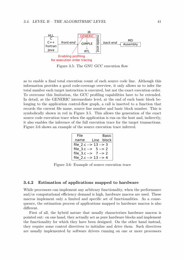
3.4. LEVEL B – THE ALGORITHMIC LEVEL 41
CC++
FortranJava
HLL GENERIC
GIMPLE
RTL
front-end back-end
middle-end
IR
AssemblyMD
Enabling profilingfor execution order tracing
Figure 3.5: The GNU GCC execution flow
as to enable a final total execution count of each source code line. Although thisinformation provides a good code-coverage overview, it only allows us to infer thetotal number each target instruction is executed, but not the exact execution order.To overcome this limitation, the GCC profiling capabilities have to be extended.In detail, at the GENERIC intermediate level, at the end of each basic block be-longing to the application control-flow graph, a call is inserted to a function thatrecords the current file name, source line number and basic block number. This issymbolically shown in red in Figure 3.5. This allows the generation of the exactsource code execution trace when the application is run on the host and, indirectly,it also enables the inference of the full execution trace for the target transactions.Figure 3.6 shows an example of the source execution trace inferred.
file_2.c --> 13 --> 3file_3.c --> 5 --> 2file_3.c --> 7 --> 2file_2.c --> 13 --> 4
Filename Line
Basicblock
Figure 3.6: Example of source execution trace
3.4.2 Estimation of applications mapped to hardwareWhile processors can implement any arbitrary functionality, when the performanceand/or computational efficiency demand is high, hardware macros are used. Thesemacros implement only a limited and specific set of functionalities. As a conse-quence, the estimation process of applications mapped to hardware macros is alsodifferent.
First of all, the hybrid nature that usually characterizes hardware macros ispointed out: on one hand, they actually act as pure hardware blocks and implementthe functionality for which they have been designed. On the other hand instead,they require some control directives to initialize and drive them. Such directivesare usually implemented by software drivers running on one or more processors

42CHAPTER 3. AN OVERVIEW OF THE FUNTIME ESTIMATION
FRAMEWORK
connected to the same SoC. The consequence is that hardware macros act both asan initiator and as a terminator. This is also the reason why the AES and the ETHblocks in Figures 3.3 to 3.8 are highlighted both in green and red.
This aspect has also to be considered when estimating the overall energy andperformance for such hardware macros. In particular, in order to include the con-tribution of the software driver in the model, the method explained above for appli-cations mapped to software could in principle be applied. However, the possibilityto do this is subordinated to the following assumption, which is unlikely to be true.This assumption is that the source code is available for the driver. This is usuallynot the case, since the driver may be covered by copyright and thus the systemarchitect would not have access to its source. Besides, assuming that the sourcecode is available, software drivers are by definition a very special piece of code,implemented to write/read to/from specific hardware. As such, it would be verydifficult to be able to run such software on the evaluation host. Finally, driversare usually required to be as optimized as possible and direct assembly coding istherefore preferred to the general C coding.
Since an IP and its own software driver are usually implemented by the sameIP provider, it makes sense that the IP provider not only implements IP energyand performance models, but that it also characterizes the software drivers for itsIPs. This characterization can be done at the granularity level of a single driverroutine. Since this same idea is applied to the operating systems characterization,the reader may want to see Section 8.2 for further details.
Estimating energy and performance for the actual functional part of the hard-ware macro can instead be enabled as follows. Recalling that estimation in Funtimerelies first of all on the ability to infer the execution trace of target transactionswithout having to implement or simulate the target architecture, two different wayscan be taken.
• If the application to be mapped to hardware shows quite a simple function-ality, the trace of transactions can be inferred through an intuitive approach.For instance, for an AES or ETH, transactions correspond to encrypt/decryptor transmit/receive operations respectively. It is also observed that the num-ber, type and order of transactions only depend in these cases on the totalvolume and the chunk of data consumed by each encrypt/decrypt or trans-mit/receive transaction. These details are known to the system architect andcan be passed to Funtime through the UCS and AS respectively. The rea-son is that the first detail is a run-time configuration parameter, while thesecond is an application-related parameter. For these two macros, a simplemathematical expression can thus be derived as a function of the parameterslisted above and the trace of transactions can be inferred. Also note that theestimation speed in this case is not proportional to the amount of data andto the size of each data chunk, as it would be instead if a simulation-basedestimation was run, but is constant. This is a critical advantage.
• If the hardware macro exhibits a more complex functionality, then another
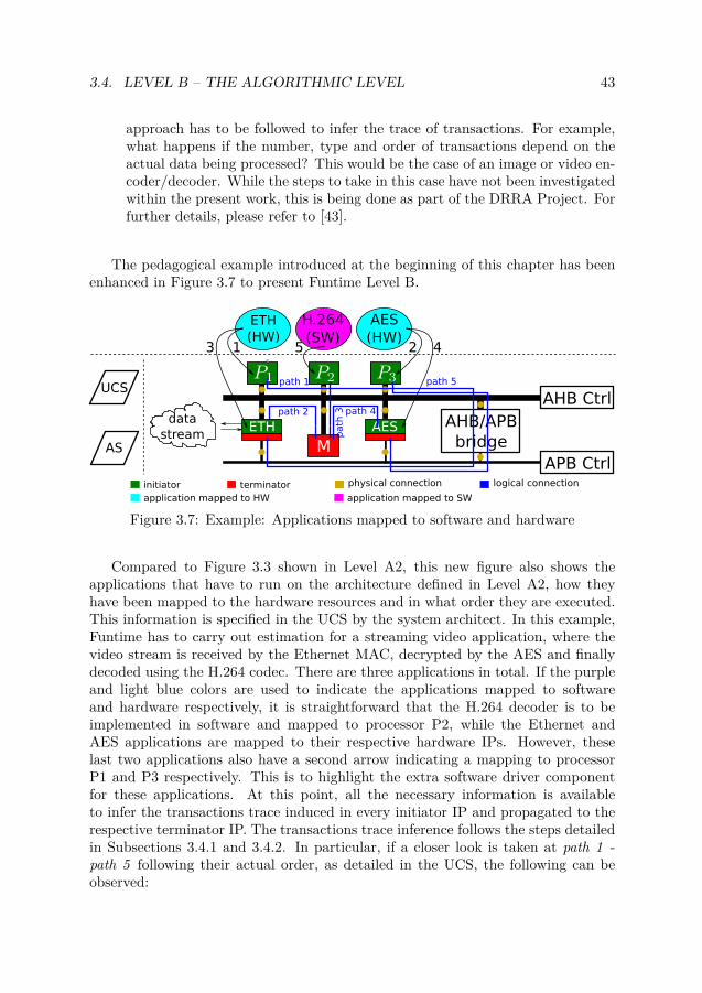
3.4. LEVEL B – THE ALGORITHMIC LEVEL 43
approach has to be followed to infer the trace of transactions. For example,what happens if the number, type and order of transactions depend on theactual data being processed? This would be the case of an image or video en-coder/decoder. While the steps to take in this case have not been investigatedwithin the present work, this is being done as part of the DRRA Project. Forfurther details, please refer to [43].
The pedagogical example introduced at the beginning of this chapter has beenenhanced in Figure 3.7 to present Funtime Level B.
AES
AHB Ctrl
APB Ctrl
AHB/APBbridge
UCS
AS M
path 1 path 5
path 2
path
3 path 4
ETH
H.264(SW)
ETH(HW)
AES(HW)
datastream
1 2 453
initiator terminator physical connection logical connection
application mapped to HW application mapped to SW
Figure 3.7: Example: Applications mapped to software and hardware
Compared to Figure 3.3 shown in Level A2, this new figure also shows theapplications that have to run on the architecture defined in Level A2, how theyhave been mapped to the hardware resources and in what order they are executed.This information is specified in the UCS by the system architect. In this example,Funtime has to carry out estimation for a streaming video application, where thevideo stream is received by the Ethernet MAC, decrypted by the AES and finallydecoded using the H.264 codec. There are three applications in total. If the purpleand light blue colors are used to indicate the applications mapped to softwareand hardware respectively, it is straightforward that the H.264 decoder is to beimplemented in software and mapped to processor P2, while the Ethernet andAES applications are mapped to their respective hardware IPs. However, theselast two applications also have a second arrow indicating a mapping to processorP1 and P3 respectively. This is to highlight the extra software driver componentfor these applications. At this point, all the necessary information is availableto infer the transactions trace induced in every initiator IP and propagated to therespective terminator IP. The transactions trace inference follows the steps detailedin Subsections 3.4.1 and 3.4.2. In particular, if a closer look is taken at path 1 -path 5 following their actual order, as detailed in the UCS, the following can beobserved:
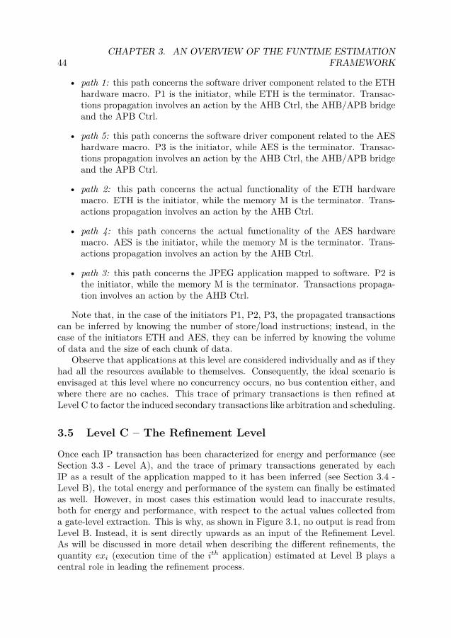
44CHAPTER 3. AN OVERVIEW OF THE FUNTIME ESTIMATION
FRAMEWORK
• path 1: this path concerns the software driver component related to the ETHhardware macro. P1 is the initiator, while ETH is the terminator. Transac-tions propagation involves an action by the AHB Ctrl, the AHB/APB bridgeand the APB Ctrl.
• path 5: this path concerns the software driver component related to the AEShardware macro. P3 is the initiator, while AES is the terminator. Transac-tions propagation involves an action by the AHB Ctrl, the AHB/APB bridgeand the APB Ctrl.
• path 2: this path concerns the actual functionality of the ETH hardwaremacro. ETH is the initiator, while the memory M is the terminator. Trans-actions propagation involves an action by the AHB Ctrl.
• path 4: this path concerns the actual functionality of the AES hardwaremacro. AES is the initiator, while the memory M is the terminator. Trans-actions propagation involves an action by the AHB Ctrl.
• path 3: this path concerns the JPEG application mapped to software. P2 isthe initiator, while the memory M is the terminator. Transactions propaga-tion involves an action by the AHB Ctrl.
Note that, in the case of the initiators P1, P2, P3, the propagated transactionscan be inferred by knowing the number of store/load instructions; instead, in thecase of the initiators ETH and AES, they can be inferred by knowing the volumeof data and the size of each chunk of data.
Observe that applications at this level are considered individually and as if theyhad all the resources available to themselves. Consequently, the ideal scenario isenvisaged at this level where no concurrency occurs, no bus contention either, andwhere there are no caches. This trace of primary transactions is then refined atLevel C to factor the induced secondary transactions like arbitration and scheduling.
3.5 Level C – The Refinement Level
Once each IP transaction has been characterized for energy and performance (seeSection 3.3 - Level A), and the trace of primary transactions generated by eachIP as a result of the application mapped to it has been inferred (see Section 3.4 -Level B), the total energy and performance of the system can finally be estimatedas well. However, in most cases this estimation would lead to inaccurate results,both for energy and performance, with respect to the actual values collected froma gate-level extraction. This is why, as shown in Figure 3.1, no output is read fromLevel B. Instead, it is sent directly upwards as an input of the Refinement Level.As will be discussed in more detail when describing the different refinements, thequantity exi (execution time of the ith application) estimated at Level B plays acentral role in leading the refinement process.

3.5. LEVEL C – THE REFINEMENT LEVEL 45
The reason why refinements are needed is that there are some implications ofsharing resources resulting from mapping, which are ignored at Level B and whichneed to be taken into account as well. Such implications are mainly related to thefact that, in reality, applications do not have all the resources always available tothemselves and often they even have to interact with other applications. The mostvisible effect of these non-idealities is a variation of the total application executionlength, in terms of number of cycles and, consequently, of the final energy too.In traditional cycle-accurate architectural simulations, this would not be an issue,as the exact number of cycles would come along as part of the simulation itself.In contrast, in the approach proposed in this thesis, this contribution needs to befactored in separately. In particular, it is demonstrated that this can be done byrefining the trace of primary transactions collected at the Level B below. Such arefinement produces what has been called secondary transactions. Accounting forthe joint contribution of both primary and secondary transactions enables accurateestimation of the total system energy and overall performance. This is shown asan output of Level C in Figure 3.1. The refinements implemented in this work areas follows.
• Transactions interdependency (Chapter 6): energy and cycles associated witha transaction often not only depend on the properties of the transaction itself,but also on the actual sequence in which transactions are issued. For exam-ple, in a processor case, its instructions execution order plays an importantrole in affecting the total application energy and cycles. Transactions inter-dependency is modeled as stall conditions, which increase the ideal executiontime.
• Caches (Chapter 6): the goal is quantifying and modeling the variation of anapplication length and energy in a system with cache, given the cache missratio and compared to the case with no cache. As opposed to the effect oftransactions interdependency, caches reduce the total number of applicationcycles, since there are fewer stall conditions caused by communication withmemory. It is pointed out that Funtime does not estimate cache miss or hitrates. This is given as input to the Funtime methodology to gauge the impacton total execution time and energy consumption.
• Bus contention (Chapter 7): in a real MPSoC, all the processors are typicallyconnected to the same bus and contention occurs when more than one applica-tion, mapped to a certain processor, requests an exclusive access to a sharedresource. The main consequence of contention is an overall degradation inperformance and an increase in energy consumption.
• Operating System (Chapter 8): although they are critical in allowing multi-tasking and in managing the sharing of hardware resources, operating systemshave an overhead, due to the execution of extra software code, both in termsof latency and energy increase.
46CHAPTER 3. AN OVERVIEW OF THE FUNTIME ESTIMATION
FRAMEWORK
Understanding in what order the different refinements should be applied is alsoimportant and is discussed in Section 3.9.
Although the approach followed in handling each refinement is different in thedetails, they all share a basic idea: characterization is done to quantify, in termsof energy and cycles, the impact of the factor to be refined; the characterizationresults are then translated into an analytical expression or an algorithm for lateruse during the estimation phase.
As for the case of the IP energy and performance models, the characterizationactivity for the Refinement Level is time-consuming, since it relies on gate-levelsimulation for accurate energy and timing extraction. However, it is justified sinceit is a one-time effort, which should be carried out by the IP provider. Note that theoperating system is also considered as an IP. Applying the refinements themselves,during the actual estimation phase by the end user, is in contrast quite fast. Moredetails about this are presented in Section 3.8.
The pedagogical example in Figure 3.8 has been extended to represent the LevelC of Funtime. Compared to Figure 3.7, the new figure points out two non-idealities,
AES
AHB Ctrl
APB Ctrl
AHB/APBbridge
UCS
AS M
path 1 path 5
path 2
path
3 path 4
ETH
H.264(SW)
ETH(HW)
AES(HW)
datastream
12
RTOS
12 2 22 2 2
initiator terminator physical connection logical connection
application mapped to HW application mapped to SW and Operating System
Figure 3.8: Example: Real scenario including RTOS, concurrent execution andcompetition for shared resources (bus)
whose impact has to be accounted for at the Refinement Level. First, the presenceof an operating system can be observed, which controls the scheduling of all theapplications mapped to software, as well as the presence of the software drivers forthe ETH and AES hardware macros. This is visualized by arrows going through

3.6. FROM SINGLE TRANSACTIONS TO A FINAL TRACE 47
the OS circle. Second, applications run concurrently, thus having to deal withbus contention issues. In particular, the applications relative to path 1 and 5 aretriggered first, then all the others are triggered together. Also note that in this casethere are three extra paths caused by the presence of applications b3, b76 and b120.
3.6 From Single Transactions to a Final Trace
This section wants to give the reader a visual example of the way a final trace ofprimary and secondary transactions can be inferred starting from single, unrelatedtransactions. As a starting point, a 2D representation of a single transaction taci isproposed in Figure 3.9. The horizontal axis shows the execution time ex, whereasthe vertical axis shows the power P . The transaction energy is therefore E = P ·ex.
Figure 3.9: Visual representation of a single transaction
Figure 3.10 shows instead how, starting from single transactions taci, Funtimeperforms the inference of a full trace of primary and secondary transactions. Thisfigure maintains the Funtime layered structure as well. Starting from Level A atthe bottom, it is assumed that a23 identifies a processor IP energy and perfor-mance model. Such a model consists of a set Ta of pre-characterized transactionstaci(E,C) with different execution time and power consumption. At Level B, thethree applications b1, b2 and b3 have been mapped to the processor IP for whichthere is model a23. By following the steps described in Section 3.4.1, Funtime in-fers a trace of primary transactions for each of the three applications. The totalprocessor execution time estimated by Funtime is thus given by summing up thetime assigned to each application. The total energy is instead given by summingup each single transaction energy. Level C takes the trace of primary transactionsand injects secondary transactions according to the rules of each refinement. Thisfigure shows three kinds of secondary transactions: stalls introduced by the trans-actions interdependency refinement in red; stalls introduced by the bus contentionrefinement in green; extra instructions introduced by the OS refinement in lightblue. The figure shows how the OS introduces context switches between the threeapplications. At this point, the total energy and execution time can be calculated.
3.7 Time Representation in Funtime
When presenting the related work and especially Transaction-Level Modeling inChapter 2, some space has been dedicated to discussing the time representation

48CHAPTER 3. AN OVERVIEW OF THE FUNTIME ESTIMATION
FRAMEWORK
Level A
Level B
Level C
Transactions interdependency ref. (stalls)
Trace of primary transactions
Bus contention ref. (stalls) OS ref. (extra instructions)
Single transactions
Trace of secondary transactions
Figure 3.10: From single transactions to a full trace of primary and secondarytransactions
in TLM. This section focuses instead on the way Funtime deals with time andcompares it to TLM. Figure 3.11 is used as a reference to discuss the comparison.The graph displayed on the left side represents the TLM case, while the one on theright represents the Funtime.
TLM Funtime
Level B
Level B
Level B
Level C
Figure 3.11: Comparison between the time representation in TLM and Funtime
Two kinds of time are considered: first, the time required by the tool to completeits estimation, which is indicated with extlm and exfuntime in the TLM and Funtimecase respectively; second, the execution time of the system under test, which is theresult of the estimation. This time is indicated as exsut.
In the figure, extlm and exfuntime are plotted on the horizontal axis, while exsut

3.7. TIME REPRESENTATION IN FUNTIME 49
is plotted on the vertical axis. In addition, both graphs show several time windowswi which correspond to different phases of the estimation tool execution time extlmor exfuntime. Note also that, due to practical drawing constraints, the graphs arenot scaled to each other as they would be in reality, and the same applies to thewidth of each wi. In reality, from the experimental results that have been carriedout, the extlm
exfuntimeratio has been found to be on average around 30.
The graph related to TLM is analyzed first. Here, two time windows are identi-fied. Window w1 corresponds to the compilation time of the application that has torun on the executable model of the target. This window only implies an incrementin extlm, but no increment in exsut. Window w2 is instead representative of thesimulation, which also corresponds to the actual estimation process. The length ofthis window is proportional to the duration of the application to be simulated. Inthis case, both extlm and exsut become incremented. However, exsut does not growlinearly, but as a step function. The height of each step y depends on the time gran-ularity chosen for the TLM model. In the case of a cycle-accurate implementation,the simulation advance in time has the granularity of a clock cycle. Conversely, inthe case of an approximately-timed implementation, which is more likely for a TLMmodel, the advance in time has a much higher granularity. The width of each stepx depends instead on the complexity of the system being simulated and can varyfor each advance of time. The higher the complexity, the longer the time extlm tosimulate a single advance in time.
Considering now the graph related to Funtime on the right, four windows areidentified. Window w1 corresponds to the compilation time of the application thathas to run on the evaluation host. Window w2 is representative of the actual timespent to execute the application on the evaluation host. As for the TLM case, thewidth of this window is proportional to the duration of the application. However,for the estimation of the same system, the width of this window in Funtime case ismuch smaller than in the TLM case, since running an application directly on thehost machine is much faster than simulating a system that runs that application.Window w3 corresponds to the time spent by Funtime to process the profiling re-sults and build a trace of primary transactions. In essence, windows w1, w2 and w3identify themselves well with the Level B of Funtime. At the end of w3, the firstestimate on the execution time (and energy) of the application being estimated isproduced. Window w4 corresponds instead to the time spent for refinement andthus to Level C. At the end of this window, the updated trace of primary and sec-ondary transactions and the final execution time exsut for the system under test areproduced. The exfuntime spent for refinement in window w4 has a minor impact onthe total value of exfuntime. The reason is that, as seen in Section 3.5, refinementsare a static activity which relies either on applying an analytical function or oniterating through an algorithm loop. The number of iterations is, however, notproportional to the application length, but to other parameters, different in eachrefinement, which allows the number of iterations to be kept low. For more details,the reader is referred to Chapters 7 and 8, where such algorithms are presented in

50CHAPTER 3. AN OVERVIEW OF THE FUNTIME ESTIMATION
FRAMEWORK
the case of the bus contention and OS refinement respectively.
3.8 Engineering Effort in Funtime
The goal of this section is to quantify the engineering effort required by the Funtimeapproach. For this purpose, the Funtime approach is considered as consisting oftwo well-defined phases: a characterization phase and an estimation phase.
The characterization phase is time-consuming and thus it requires a large en-gineering effort. This phase includes for example implementing IP energy andperformance models (at Level A). As summarized in Section 3.3, the creation ofIP models implies characterizing each IP transaction for energy and number ofcycles. This phase also includes implementing the refinements (at Level C). Assummarized in Section 3.5, refinements consist of a characterization phase as well,where the impact of a certain element (transactions interdependency, caches, buscontention and OS) is quantified and translated into an analytical expression oran algorithm for later use during the estimation phase. None of these activities iscarried out by the end user of Funtime though. In fact, the engineering effort of thischaracterization phase is shared among the different IP providers when creating IPenergy and performance models or implementing the refinements, including the OSrefinement, which can also be considered as an IP. Although time-consuming, thischaracterization phase is justified for the following three reasons: first, it is doneonly once; second, it gives high accuracy to the whole Funtime framework since itis carried out at the gate level; third, it is a shared activity, which helps to bringthe engineering effort down.
As opposed to the characterization phase, the estimation phase is very fast andinteractive, and the engineering effort minimal. In fact, this phase involves Level Band C of Funtime. As seen before, Level B produces a trace of primary transactionsafter running an instrumented application on the evaluation host; Level C adds thecontribution of the secondary transactions by applying the refinement implementedduring the characterization phase. What happens in the evaluation phase is theresponsibility of the system architect.
Based on these considerations, the overall engineering effort required by theFuntime approach is low, and in general lower than the effort required by TLM. Thereason is that TLM also relies on the availability of IP energy models if the systemarchitect expects to get energy numbers out of the TLM simulation. However, inaddition to this, TLM also requires the time-consuming activity of using a HLL tobuild executable models of the target architecture. This step, which is absent inFuntime, is not negligible within the overall design time budget.
3.9 Refinements Order and Interaction
In Section 3.5, the importance of the refinement activity has been justified and anoverview of the refinements implemented in the context of the present work has

3.9. REFINEMENTS ORDER AND INTERACTION 51
been presented. So far, refinements have been presented individually. In practice,however, the refinement order is significant and impacts the estimation accuracy.The following discussion presents this aspect of the refinement process in Funtime.The same MPSoC example presented throughout Sections 3.3 to 3.5 is used hereas a reference architecture.
The initial assumption is made that the reference MPSoC has a single appli-cation mapped on itself and running on one processor. It is also assumed thatexecuting this application only implies write/read operations to/from a memoryconnected to the MPSoC shared bus. In this case, no bus contention is expected,since this processor is the only active initiator. In addition, there is no need toassume any running Operating System either, which means that the OS overheadcan be neglected. The energy and execution time of this unique application canthus be estimated. However, as mentioned in Section 3.5, in doing this it is notpossible just to sum up the energy E and cycles C associated with each individualtransaction taci(E,C): it is also necessary to account for the extra cycles (stallevents) caused by the different order in which transactions – processor instructionsin this case – can be triggered.
The transactions interdependency refinement, which is discussed in Chapter 6,is thus the first refinement to be applied. Its action is symbolically shown in Fig-ure 3.12 and consists of the synthetic injection of extra cycles (in red) after eachtransaction.
TransactionsInterdependency
Refinement
Figure 3.12: First refinement: transaction interdependency
When modeling processor transactions and when applying the transactions in-terdependency refinement, it makes sense to assume either the case where the cachemiss ratio MR = 100% or MR = 0%. Besides, both cases can in principle berepresentative of real-case scenarios. The case of MR = 100% can indicate an ar-chitecture where no cache is used, which is common in systems with hard real-timeconstraints, since they have to be as predictable as possible. Conversely, the case ofMR ' 0%, especially when looking at the instruction cache, can occur when run-ning very regular applications, such as algorithms that often iterate a large numberof times through the same code loop.
The present work, as detailed in Chapter 4, shows how to characterize a pro-cessor assuming both the case of MR = 100% and MR = 0%. Together with thetransactions interdependency refinement, the cache refinement allows us to get thetransactions trace shown on the right side of Figure 3.12. However, in reality, thereare also many cases where intermediate MR values are possible. Accounting forthis possibility is part of the cache refinement, which is discussed in Chapter 6 and

52CHAPTER 3. AN OVERVIEW OF THE FUNTIME ESTIMATION
FRAMEWORK
is thus the second refinement to be applied.In more detail, the cache refinement aims at quantifying and modeling the
variation of an application length and energy in a system with cache, given thecache miss ratio. In principle, this variation can be predicted with respect to thecase of MR = 100% or MR = 0%. The present work uses the case of MR = 100%as a reference. In addition, the variation prediction is done so far with respect to anentire application, and not to its single transactions. The reason is that, to makethis second option possible, it would be necessary to simulate the application onthe target, in order to have the details on which transactions actually cause a cachehit or miss. However, this is not a viable approach, since it would go against thewhole idea Funtime rests on.
Note that the transactions interdependency refinement and the cache refine-ment, i.e. the first and second refinement to be applied, act on individual appli-cations and do not depend on other refinements. In fact, even if in principle thecache miss ratio would be affected by the effects of bus contention and operatingsystem overhead, in Funtime the miss ratio is passed as an input parameter to theUCS by the system designer and the cache refinement is applied as a function ofthis value.
Considering now that the MPSoC can run multiple applications in parallel,where more than one application can be mapped to the same processor, and wherean OS is used to control their execution, the bus contention refinement and theoperating system refinement also start playing an important role. This is the caserepresented in Figure 3.8. The bus contention refinement aims at predicting theextra cycles (stall events) and energy introduced by bus contention based on thenumber of initiators sharing the same bus and on the distinction between store/load-related instructions vs. other instructions. The OS refinement instead aims atpredicting the extra cycles and energy introduced by the presence of an OS.
Unlike the two previous refinements, these refinements have the following de-pendencies. First, they depend on the previous refinements. Intuitively, in fact, theprobability of bus contention events or the number of context switches is likely toincrease along with the application’s execution length, where the estimated applica-tion length is a function of the transactions interdependency and cache refinements.Second, the OS and bus contention refinements also depend on each other. In fact,the OS itself introduces extra instructions, which increase the number of memoryaccesses and thus the probability of bus contention. In turn, a higher bus contentionincreases the overall applications time, thus leading to more context switches/clocktick interrupts and, in general, to a higher OS overhead. This again will affect thebus contention probabilities, and so on.
For these reasons, the order in which the bus contention refinement and the OSrefinement have to be applied cannot be sequential as for the previous refinements.Instead, an iterative process has to be adopted.
Chapter 4
Level A1 – Implementing IPEnergy and Performance Models:The Leon3 Processor Case
This chapter presents a methodology to create the energy and performance model foran IP corresponding to the Level A1 in the Funtime framework. This activity is timeconsuming, but it is justified as being a one-time activity that is used by multipleend-users and is intended to be performed by the IP provider. The methodologyis applied to the Leon3 as a case study. It is also shown that an accuracy can beachieved within 15% of gate-level measurement. The work presented in this chapteris based on the author’s publication in [53].
4.1 Introduction
As discussed in Section 3.3.1, creating IP energy and performance models makessense since, although time-consuming, it is done only once by the IP provider. Thisis possible thanks to the spreading of the Design&Reuse concept, which empha-sizes that reusing already existing IPs is more efficient than writing new ones fromscratch. This modeling activity relies on characterizing each IP transaction in termsof energy in Joules and performance in cycles, where each transaction correspondsto one IP functionality. Examples of transactions can be write/read for a bus,code/decode for a codec, transmit/receive for an I/O, the full instructions set fora processor, or the coarse-grain routines of an operating system.
The activity of building individual IP energy and performance models is partof the Level A1 of the Funtime methodology. Such models are then collected in adatabase and used by the above Level A2. This is shown in Figure 4.1.
In this chapter, the creation of an energy and performance model for the Leon3processor is used as a case study. The Leon3 model proposed in the present workis based on instruction-level characterization. Although this modeling approach
53

54CHAPTER 4. LEVEL A1 – IMPLEMENTING IP ENERGY AND
PERFORMANCE MODELS: THE LEON3 PROCESSOR CASE
A1 - Individual IPs
:= Database of IP energy and performance models
Figure 4.1: The IP Level – Individual IPs (Level A1)
for processors has already been adopted in the past, as reviewed in Section 4.2, afurther contribution is made in the present work through the following:
• instructions interdependency: the energy of an instruction is heavily depen-dent on the actual sequence in which instructions have been issued. Forthis reason, two different energy models are implemented and compared: onewhere characterization is done on a single instruction basis, the other wherecharacterization is done on pairs of instructions.
• data switching activity: it is shown that instructions energy varies signifi-cantly depending on the switching activity of the data that the instructionhandles. As a consequence, a sensible way is proposed to model energy ac-counting for this aspect also.
• registers correlation: it is shown that, for a subset of instructions pairs, whentwo subsequent instructions use at least one same register, the execution timeincreases and, consequently, the energy consumption changes too.
The model is validated on a set of real applications by comparing its estimates tothe numbers extracted from gate-level simulation. An error is obtained within 6%and 12% for the models applied to Leon3 configurations without and with cacherespectively.
4.2 Related Work
Building processor energy models has been the focus of several research groups. In[51], the authors describe a method to create instruction-level power models basedon directly measuring the average current from the board. In order to make thismeasurement more accurate, they suggest executing a sequence where the sameinstruction under test (IUT) is repeated several times in a row, and taking theaverage value.
In [70], the authors characterize instructions for energy by executing a prede-fined sequence of instructions, where the IUT is always interleaved by a certainnumber of NOPs. Besides, measurements are in this case carried out from back-annotated gate-level simulation. The approach presented in this thesis, as detailedin Section 4.4, is similar, but enhanced to consider pairs of instructions, in order tomodel instructions interdependency on energy.
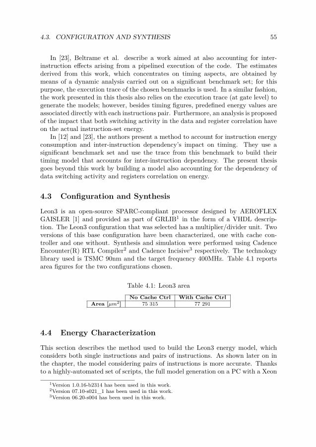
4.3. CONFIGURATION AND SYNTHESIS 55
In [23], Beltrame et al. describe a work aimed at also accounting for inter-instruction effects arising from a pipelined execution of the code. The estimatesderived from this work, which concentrates on timing aspects, are obtained bymeans of a dynamic analysis carried out on a significant benchmark set; for thispurpose, the execution trace of the chosen benchmarks is used. In a similar fashion,the work presented in this thesis also relies on the execution trace (at gate level) togenerate the models; however, besides timing figures, predefined energy values areassociated directly with each instructions pair. Furthermore, an analysis is proposedof the impact that both switching activity in the data and register correlation haveon the actual instruction-set energy.
In [12] and [23], the authors present a method to account for instruction energyconsumption and inter-instruction dependency’s impact on timing. They use asignificant benchmark set and use the trace from this benchmark to build theirtiming model that accounts for inter-instruction dependency. The present thesisgoes beyond this work by building a model also accounting for the dependency ofdata switching activity and registers correlation on energy.
4.3 Configuration and Synthesis
Leon3 is an open-source SPARC-compliant processor designed by AEROFLEXGAISLER [1] and provided as part of GRLIB1 in the form of a VHDL descrip-tion. The Leon3 configuration that was selected has a multiplier/divider unit. Twoversions of this base configuration have been characterized, one with cache con-troller and one without. Synthesis and simulation were performed using CadenceEncounter(R) RTL Compiler2 and Cadence Incisive3 respectively. The technologylibrary used is TSMC 90nm and the target frequency 400MHz. Table 4.1 reportsarea figures for the two configurations chosen.
Table 4.1: Leon3 area
No Cache Ctrl With Cache CtrlArea [µm2] 75 315 77 291
4.4 Energy Characterization
This section describes the method used to build the Leon3 energy model, whichconsiders both single instructions and pairs of instructions. As shown later on inthe chapter, the model considering pairs of instructions is more accurate. Thanksto a highly-automated set of scripts, the full model generation on a PC with a Xeon
1Version 1.0.16-b2314 has been used in this work.2Version 07.10-s021_1 has been used in this work.3Version 06.20-s004 has been used in this work.

56CHAPTER 4. LEVEL A1 – IMPLEMENTING IP ENERGY AND
PERFORMANCE MODELS: THE LEON3 PROCESSOR CASE
processor @2.5GHz takes five hours for the the 1-instruction-based case and around10 days for the 2-instruction-based case.
4.4.1 1-instruction-based modelThe main idea is to isolate and extract energy and number of cycles associatedwith each processor instruction for the selected configurations. Since no Floating-Point Unit (FPU) or Co-Processor (CP) are provided within the present work, thecorresponding instructions are not part of the model.
The method used for characterization relies on executing for 100 consecutivetimes a basic sequence composed of five NOPs, one instruction under test (IUT)and five NOPs, for a total of 1100 executed instructions, as shown in Expression4.1.
100× (5 ·NOP, IUT, 5 ·NOP ) (4.1)
The reason behind choosing such a sequence as a reference is to be able to isolateeach IUT, and this operation is easier if the IUT is surrounded by NOP instructions,which in principle do not have any active functionality, do not show interdependencyand consume the least energy. In effect, in this way each IUT is isolated by 10 NOPs.However, since the pipeline is made of seven stages, seven NOPs would probablyhave been enough.
The basic sequence is then repeated 100 times. The reason is to find a reasonableaverage energy value that can be considered statistically valid. The higher thenumber of iterations, the better the result from a statistical perspective, but theoverhead introduced by the increased simulation time also needs to be considered.That is why the number of iterations is limited to 100.
In addition, in each iteration, different registers are used for the same IUT;this is to keep the correlation between subsequent executions as low as possible.However, this does not apply to instructions that do not operate on any register,like NOP. Correlation between instruction energy and registers usage is dealt within Section 4.6.
The first selected IUT is the NOP itself. From Expression 4.1, this leads to theexecution of 1100 NOPs, for which energy is calculated. The energy and cycles fora single NOP are therefore given by Eq. 4.2 and Eq. 4.3 respectively.
ENOP = E1100_NOP
1100 (4.2)
CNOP = tstop − tstart1100 · Tclk
(4.3)
In Eq. 4.3, tstart and tstop correspond to the initial and final gate-level simulationtime for the 100-time loop of the basic sequence.
Once the energy of a single NOP is known, calculating the energy for the otherIUTs is quite straightforward: since in these cases 100 IUTs and 1000 NOPs are
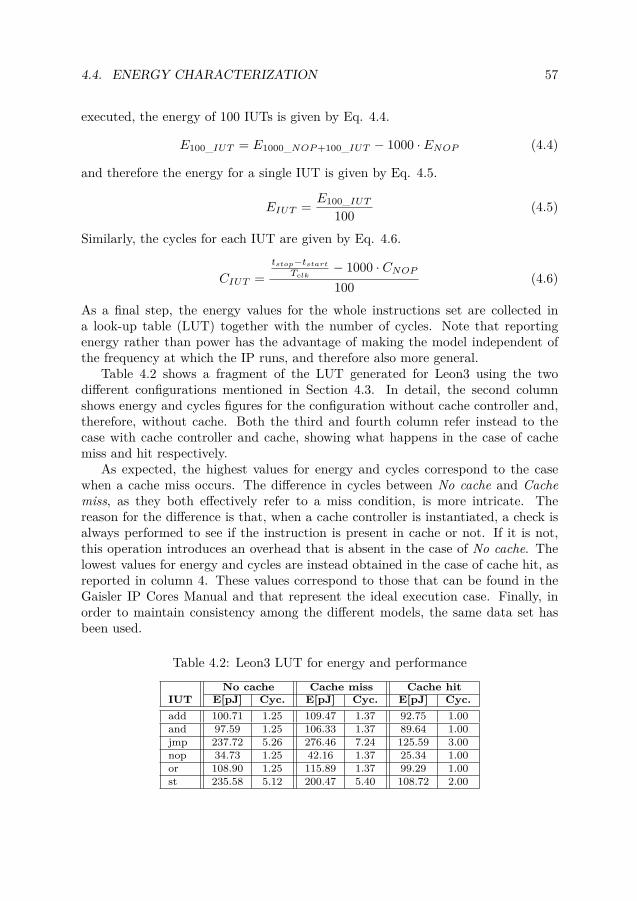
4.4. ENERGY CHARACTERIZATION 57
executed, the energy of 100 IUTs is given by Eq. 4.4.
E100_IUT = E1000_NOP+100_IUT − 1000 · ENOP (4.4)
and therefore the energy for a single IUT is given by Eq. 4.5.
EIUT = E100_IUT
100 (4.5)
Similarly, the cycles for each IUT are given by Eq. 4.6.
CIUT =tstop−tstart
Tclk− 1000 · CNOP100 (4.6)
As a final step, the energy values for the whole instructions set are collected ina look-up table (LUT) together with the number of cycles. Note that reportingenergy rather than power has the advantage of making the model independent ofthe frequency at which the IP runs, and therefore also more general.
Table 4.2 shows a fragment of the LUT generated for Leon3 using the twodifferent configurations mentioned in Section 4.3. In detail, the second columnshows energy and cycles figures for the configuration without cache controller and,therefore, without cache. Both the third and fourth column refer instead to thecase with cache controller and cache, showing what happens in the case of cachemiss and hit respectively.
As expected, the highest values for energy and cycles correspond to the casewhen a cache miss occurs. The difference in cycles between No cache and Cachemiss, as they both effectively refer to a miss condition, is more intricate. Thereason for the difference is that, when a cache controller is instantiated, a check isalways performed to see if the instruction is present in cache or not. If it is not,this operation introduces an overhead that is absent in the case of No cache. Thelowest values for energy and cycles are instead obtained in the case of cache hit, asreported in column 4. These values correspond to those that can be found in theGaisler IP Cores Manual and that represent the ideal execution case. Finally, inorder to maintain consistency among the different models, the same data set hasbeen used.
Table 4.2: Leon3 LUT for energy and performance
No cache Cache miss Cache hitIUT E[pJ] Cyc. E[pJ] Cyc. E[pJ] Cyc.add 100.71 1.25 109.47 1.37 92.75 1.00and 97.59 1.25 106.33 1.37 89.64 1.00jmp 237.72 5.26 276.46 7.24 125.59 3.00nop 34.73 1.25 42.16 1.37 25.34 1.00or 108.90 1.25 115.89 1.37 99.29 1.00st 235.58 5.12 200.47 5.40 108.72 2.00

58CHAPTER 4. LEVEL A1 – IMPLEMENTING IP ENERGY AND
PERFORMANCE MODELS: THE LEON3 PROCESSOR CASE
4.4.2 2-instruction-based modelThe method used for characterization is in principle similar to that presented inSubsection 4.4.1, with the difference that now a sequence of two IUTs is consideredinstead of one. The basic sequence is shown in Expression 4.7.
100× (5 ·NOP, IUT1, IUT2, 5 ·NOP ) (4.7)
Table 4.3 reports a few examples where the energy is compared between the 1-instruction-based and the 2-instruction-based model for the case of cache hit. Sim-ilarly, Figure 4.2 shows the overall energy difference for all the possible 2-tuples ofinstructions, which means around 6000 pairs. In 90% of the cases, the energy of a2-tuple is lower than the energy given by summing single instructions energy, andthe average difference is around -12%. The methodology proposed in the presentwork is, however, general and based on the actual measurement of increment anddecrement in energy and is thus not dependent on a specific architecture property.No table is shown comparing the number of cycles extracted in the two approaches,since they are identical.
Table 4.3: Energy models: 1-instr. vs. 2-instr.
1-instr-model 2-instr-modelIUT E[pJ] Sum IUT_1-2 E[pJ] Diff.[%]add 92.75 182.39 add_and 120.65 -33.85and 89.64and 89.64 188.93 and_or 127.72 -32.40or 99.29ld 75.17 168.30 ld_xor 128.24 -23.81xor 93.13
Figure 4.2: EnIUT1+EnIUT2 versus EnIUT1_IUT2
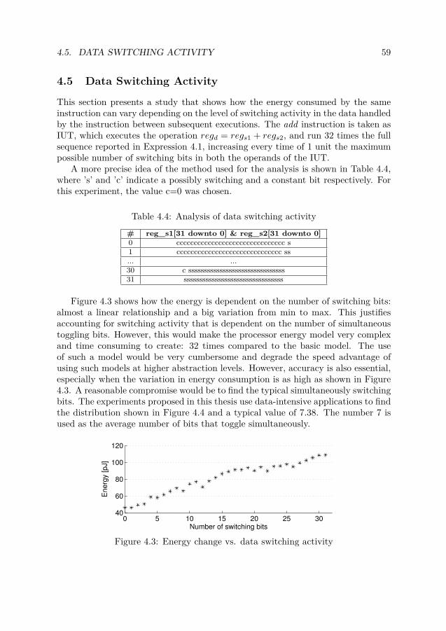
4.5. DATA SWITCHING ACTIVITY 59
4.5 Data Switching Activity
This section presents a study that shows how the energy consumed by the sameinstruction can vary depending on the level of switching activity in the data handledby the instruction between subsequent executions. The add instruction is taken asIUT, which executes the operation regd = regs1 + regs2, and run 32 times the fullsequence reported in Expression 4.1, increasing every time of 1 unit the maximumpossible number of switching bits in both the operands of the IUT.
A more precise idea of the method used for the analysis is shown in Table 4.4,where ’s’ and ’c’ indicate a possibly switching and a constant bit respectively. Forthis experiment, the value c=0 was chosen.
Table 4.4: Analysis of data switching activity
# reg_s1[31 downto 0] & reg_s2[31 downto 0]0 ccccccccccccccccccccccccccccccc s1 cccccccccccccccccccccccccccccc ss... ...30 c sssssssssssssssssssssssssssssss31 ssssssssssssssssssssssssssssssss
Figure 4.3 shows how the energy is dependent on the number of switching bits:almost a linear relationship and a big variation from min to max. This justifiesaccounting for switching activity that is dependent on the number of simultaneoustoggling bits. However, this would make the processor energy model very complexand time consuming to create: 32 times compared to the basic model. The useof such a model would be very cumbersome and degrade the speed advantage ofusing such models at higher abstraction levels. However, accuracy is also essential,especially when the variation in energy consumption is as high as shown in Figure4.3. A reasonable compromise would be to find the typical simultaneously switchingbits. The experiments proposed in this thesis use data-intensive applications to findthe distribution shown in Figure 4.4 and a typical value of 7.38. The number 7 isused as the average number of bits that toggle simultaneously.
0 5 10 15 20 25 3040
60
80
100
120
Number of switching bits
En
erg
y [
pJ]
Figure 4.3: Energy change vs. data switching activity

60CHAPTER 4. LEVEL A1 – IMPLEMENTING IP ENERGY AND
PERFORMANCE MODELS: THE LEON3 PROCESSOR CASE
Figure 4.4: Distribution of simultaneously switching bits per register
4.6 Registers Correlation
This section presents an analysis to evaluate the impact of registers correlationbetween two instructions in sequence on the energy consumption of an instructionspair. The modeling sequence reported in Expression 4.7 is used. Specifically, forregisters correlation the case is meant where the destination register for the firstinstruction becomes a source register for the second instruction. An example isgiven below:
add reg1 + reg2 -> reg3sub reg3 + reg4 -> reg5
Table 4.5 compares the time and energy variations caused by registers correlation tothe case where correlation is not present. This table also refers to the case of cachehit. The table is further split horizontally into two groups: the upwards portionrefers to the case where correlation increases the number of cycles. This increasecan be justified by using the ld_add pair as an example: since one of the twooperands on which the add has to operate is not available until the ld is completed,no advantage can be taken by the pipelined architecture of the processor. As aconsequence, two extra cycles are required for the add to complete.
In principle, this reasoning also applies to the downwards portion of the table.Here however, registers correlation does not affect the execution time. This happensbecause the first instruction in the pair takes only one cycle to execute, which is tooshort a time to allow any level of parallelization, even in the case that no correlationbetween registers exists.
The real occurrence of registers correlation has been estimated on the same testapplications used in Section 4.5. The results show that such a correlation is presenton average for 50% of the executed instructions, despite a relatively high standarddeviation σ '13%. It is therefore sensible to believe that also factoring in thisaspect when building the energy model would increase the estimation accuracy.However, since this work is not yet complete, the present thesis validates a Leon3model that does not yet account for registers correlation.

4.7. VALIDATING THE LEON3 MODEL ESTIMATION ACCURACY 61
Table 4.5: Registers correlation analysis
With corr. No corr. CyclesPair E[pJ] Cyc. E[pJ] Cyc. Diff.
ld_add 269.66 4 125.53 2 +2smul_smul 332.46 11 495.41 10 +1xor_st 180.85 3 184.00 3 ±0sll_add 136.20 2 141.34 2 ±0
Table 4.6: Leon3 energy models (1-instr-based with/without data dependency) vs.gate-level energy measurement (no cache)
FFT Quicksort Fibonacci# Instructions 1 371 584 4 008 651 1 585 313# Cycles 6 485 094 31 649 232 13 902 019Real energy [mJ] 0.2396 1.1508 0.4906
with data dependency(toggle = 7 bits)
Estimated instructions energy [mJ] 0.1388 0.5209 0.1917Estimated stalls energy [mJ] 0.1319 0.6766 0.3218Estimated total energy [mJ] 0.2706 1.1975 0.5135Error [%] +12.96 +4.05 +4.67
without data dependency(toggle = 15 bits)
Estimated instructions energy [mJ] 0.1565 0.5463 0.1981Estimated stalls energy [mJ] 0.1319 0.6766 0.3218Estimated total energy [mJ] 0.2884 1.2228 0.5199Error [%] +20.37 +6.26 +5.98
Viterbi Queens Dhrystone MD5# Instructions 2 452 903 4 266 783 1 950 813 1 802 380# Cycles 17 511 989 24 193 885 15 938 144 14 428 588Real energy [mJ] 0.6250 0.8571 0.5641 0.5228
with data dependency(toggle = 7 bits)
Estimated instructions energy [mJ] 0.3009 0.4389 0.2581 0.2192Estimated stalls energy [mJ] 0.3871 0.5166 0.3529 0.3302Estimated total energy [mJ] 0.6880 0.9555 0.6110 0.5494Error [%] +10.08 +11.48 +8.31 +4.90
without data dependency(toggle = 15 bits)
Estimated instructions energy [mJ] 0.3247 0.4884 0.2711 0.2346Estimated stalls energy [mJ] 0.3871 0.5166 0.3529 0.3302Estimated total energy [mJ] 0.7118 1.0050 0.6240 0.5648Error [%] +13.89 +17.25 +10.61 +7.84
4.7 Validating the Leon3 Model Estimation Accuracy
Validation for the Leon3 model has been carried out on a set of common benchmarkapplications and takes gate-level extraction as a reference. The accuracy of theLeon3 modeling approach has been tested for a processor with and without cache(4k I/D cache). When applying the models, the estimated number of total cyclesis always lower than the actual one extracted from gate-level simulation. Thisdifference has been associated with the occurrence of stall conditions, whose energyper cycle Estall has been modeled according to Eq. 4.8:
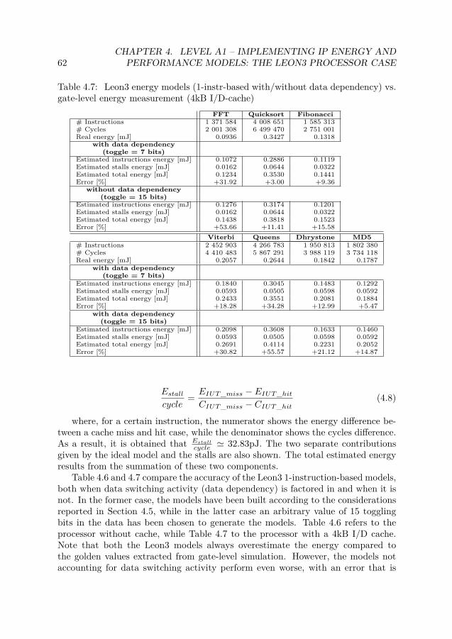
62CHAPTER 4. LEVEL A1 – IMPLEMENTING IP ENERGY AND
PERFORMANCE MODELS: THE LEON3 PROCESSOR CASE
Table 4.7: Leon3 energy models (1-instr-based with/without data dependency) vs.gate-level energy measurement (4kB I/D-cache)
FFT Quicksort Fibonacci# Instructions 1 371 584 4 008 651 1 585 313# Cycles 2 001 308 6 499 470 2 751 001Real energy [mJ] 0.0936 0.3427 0.1318
with data dependency(toggle = 7 bits)
Estimated instructions energy [mJ] 0.1072 0.2886 0.1119Estimated stalls energy [mJ] 0.0162 0.0644 0.0322Estimated total energy [mJ] 0.1234 0.3530 0.1441Error [%] +31.92 +3.00 +9.36
without data dependency(toggle = 15 bits)
Estimated instructions energy [mJ] 0.1276 0.3174 0.1201Estimated stalls energy [mJ] 0.0162 0.0644 0.0322Estimated total energy [mJ] 0.1438 0.3818 0.1523Error [%] +53.66 +11.41 +15.58
Viterbi Queens Dhrystone MD5# Instructions 2 452 903 4 266 783 1 950 813 1 802 380# Cycles 4 410 483 5 867 291 3 988 119 3 734 118Real energy [mJ] 0.2057 0.2644 0.1842 0.1787
with data dependency(toggle = 7 bits)
Estimated instructions energy [mJ] 0.1840 0.3045 0.1483 0.1292Estimated stalls energy [mJ] 0.0593 0.0505 0.0598 0.0592Estimated total energy [mJ] 0.2433 0.3551 0.2081 0.1884Error [%] +18.28 +34.28 +12.99 +5.47
with data dependency(toggle = 15 bits)
Estimated instructions energy [mJ] 0.2098 0.3608 0.1633 0.1460Estimated stalls energy [mJ] 0.0593 0.0505 0.0598 0.0592Estimated total energy [mJ] 0.2691 0.4114 0.2231 0.2052Error [%] +30.82 +55.57 +21.12 +14.87
Estallcycle
= EIUT_miss − EIUT_hit
CIUT_miss − CIUT_hit(4.8)
where, for a certain instruction, the numerator shows the energy difference be-tween a cache miss and hit case, while the denominator shows the cycles difference.As a result, it is obtained that Estall
cycle ' 32.83pJ. The two separate contributionsgiven by the ideal model and the stalls are also shown. The total estimated energyresults from the summation of these two components.
Table 4.6 and 4.7 compare the accuracy of the Leon3 1-instruction-based models,both when data switching activity (data dependency) is factored in and when it isnot. In the former case, the models have been built according to the considerationsreported in Section 4.5, while in the latter case an arbitrary value of 15 togglingbits in the data has been chosen to generate the models. Table 4.6 refers to theprocessor without cache, while Table 4.7 to the processor with a 4kB I/D cache.Note that both the Leon3 models always overestimate the energy compared tothe golden values extracted from gate-level simulation. However, the models notaccounting for data switching activity perform even worse, with an error that is
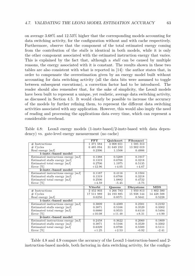
4.7. VALIDATING THE LEON3 MODEL ESTIMATION ACCURACY 63
on average 3.68% and 12.53% higher that the corresponding models accounting fordata switching activity, for the configuration without and with cache respectively.Furthermore, observe that the component of the total estimated energy comingfrom the contribution of the stalls is identical in both models, while it is onlythe other component associated with the estimated instruction energy that varies.This is explained by the fact that, although a stall can be caused by multiplereasons, the energy associated with it is constant. The results shown in these twotables are also consistent with what is reported in [14]: the author states that, inorder to compensate the overestimation given by an energy model built withoutaccounting for data switching activity (all the data bits were assumed to togglebetween subsequent executions), a correction factor had to be introduced. Thereader should also remember that, for the sake of simplicity, the Leon3 modelshave been built to represent a unique, yet realistic, average data switching activity,as discussed in Section 4.5. It would clearly be possible to increase the accuracyof the models by further refining them, to represent the different data switchingactivities associated with any application. However, this would also imply the needof reading and processing the applications data every time, which can represent aconsiderable overhead.
Table 4.8: Leon3 energy models (1-instr-based/2-instr-based with data depen-dency) vs. gate-level energy measurement (no cache)
FFT Quicksort Fibonacci# Instructions 1 371 584 4 008 651 1 585 313# Cycles 6 485 094 31 649 232 13 902 019Real energy [mJ] 0.2396 1.1508 0.4906
1-instr.-based modelEstimated instructions energy [mJ] 0.1388 0.5209 0.1917Estimated stalls energy [mJ] 0.1319 0.6766 0.3218Estimated total energy [mJ] 0.2706 1.1975 0.5135Error [%] +12.96 +4.05 +4.67
2-instr.-based modelEstimated instructions energy [mJ] 0.1187 0.4116 0.1504Estimated stalls energy [mJ] 0.1319 0.6766 0.3218Estimated total energy [mJ] 0.2506 1.0882 0.4722Error [%] +4.59 -5.45 -3.75
Viterbi Queens Dhrystone MD5# Instructions 2 452 903 4 266 783 1 950 813 1 802 380# Cycles 17 511 989 24 193 885 15 938 144 14 428 588Real energy [mJ] 0.6250 0.8571 0.5641 0.5228
1-instr.-based modelEstimated instructions energy [mJ] 0.3009 0.4389 0.2581 0.2192Estimated stalls energy [mJ] 0.3871 0.5166 0.3529 0.3302Estimated total energy [mJ] 0.6880 0.9555 0.6110 0.5494Error [%] +10.08 +11.48 +8.31 +4.90
2-instr.-based modelEstimated instructions energy [mJ] 0.2458 0.3622 0.2060 0.1809Estimated stalls energy [mJ] 0.3871 0.5166 0.3529 0.3302Estimated total energy [mJ] 0.6329 0.8788 0.5589 0.5111Error [%] +1.25 +2.53 -0.92 -2.41
Table 4.8 and 4.9 compare the accuracy of the Leon3 1-instruction-based and 2-instruction-based models, both factoring in data switching activity, for the configu-

64CHAPTER 4. LEVEL A1 – IMPLEMENTING IP ENERGY AND
PERFORMANCE MODELS: THE LEON3 PROCESSOR CASE
ration without and with cache respectively. It can be noticed that the 2-instruction-based model is in general more accurate than the 1-instruction-based one, witha margin of error <6% and <12% compared to gate level, for the configurationwithout and with cache respectively. Besides, the model based on a single instruc-tion always overestimates the actual energy, making a worst-case error up to '32%when considering the configuration with cache; compared to the 2-instruction-basedmodel, it also overestimates on average '8.65% and '17.45% for the configurationwithout and with cache respectively, which is consistent with what has been re-ported in Subsection 4.4.2.
Table 4.9: Leon3 energy models (1-instr-based/2-instr-based with data depen-dency) vs. gate-level energy measurement (4kB I/D-cache)
FFT Quicksort Fibonacci# Instructions 1 371 584 4 008 651 1 585 313# Cycles 2 001 308 6 499 470 2 751 001Real energy [mJ] 0.0936 0.3427 0.1318
1-instr.-based modelEstimated instructions energy [mJ] 0.1072 0.2886 0.1119Estimated stalls energy [mJ] 0.0162 0.0644 0.0322Estimated total energy [mJ] 0.1234 0.3530 0.1441Error [%] +31.92 +3.00 +9.36
2-instr.-based modelEstimated instructions energy [mJ] 0.0843 0.2380 0.0985Estimated stalls energy [mJ] 0.0162 0.0644 0.0322Estimated total energy [mJ] 0.1005 0.3024 0.1307Error [%] +7.37 -11.75 -0.82
Viterbi Queens Dhrystone MD5# Instructions 2 452 903 4 266 783 1 950 813 1 802 380# Cycles 4 410 483 5 867 291 3 988 119 3 734 118Real energy [mJ] 0.2057 0.2644 0.1842 0.1787
1-instr.-based modelEstimated instructions energy [mJ] 0.1840 0.3045 0.1483 0.1292Estimated stalls energy [mJ] 0.0593 0.0505 0.0598 0.0592Estimated total energy [mJ] 0.2433 0.3551 0.2081 0.1884Error [%] +18.28 +34.28 +12.99 +5.47
2-instr.-based modelEstimated instructions energy [mJ] 0.1472 0.2333 0.1224 0.1045Estimated stalls energy [mJ] 0.0593 0.0505 0.0598 0.0592Estimated total energy [mJ] 0.2065 0.2839 0.1822 0.1638Error [%] +0.42 +7.36 -1.10 -8.33
From these results, it is possible to draw two important conclusions: first, ac-counting for data switching activity helps improve the overall model accuracy; sec-ond, the 2-instruction-based model is reasonably accurate and, on average, signifi-cantly more accurate than the 1-instruction-based model, which justifies the extraeffort in making it.
It would also be interesting to compare the results presented in this thesis withsomeone else’s, but at present no equivalent work has been found to compare with.

4.8. SUMMARY 65
4.8 Summary
This chapter has described a methodology to implement an energy and performancemodel for a processor, a Leon3 in this case, based on instruction-level characteri-zation. Specifically, the impact of instructions interdependency on energy has beeninvestigated by building an energy model with two degrees of accuracy, one basedon characterizing each single instruction, the other based on characterizing instruc-tions pairs. The study also takes into account the effect that data switching activityand registers correlation have on energy. Validation has then been done against gatelevel for estimation accuracy, incurring an error within 6% and 12% for the modelsapplied to the configurations without and with cache respectively.
Note that, thanks to the high level of automation applied to the energy mod-els generation process, this approach is quite general and can therefore be easilyadapted and used on different architectures. More important, this modeling ex-ercise has the goal of showing how an IP energy and performance model can beimplemented in practice.
Another example of how an IP energy and performance model can be built fora NoC switch is presented in the previous work published by the author in [56]. Inthis case, due to the different nature of the IP, the model has been expressed usingan analytical representation instead of LUTs.

Chapter 5
Level A2 – Modeling IPsComposite Transactions
This chapter shows how it is possible to model composite transactions. This activityis necessary in order to be able to identify and account for the components repre-senting the external communication aspects. These components are architecture-dependent and change when the system architecture changes. The activity of mod-eling composite transactions is illustrated in this chapter by making a switch froman AHB bus-based SoC to a NoC-based SoC. The model, when adapted for NoC,has an accuracy within 10% compared to the gate-level measurement.
5.1 Introduction
Subsection 3.3.2 has discussed the distinction in Funtime between simple and com-posite transactions. While simple transactions are internal and can be characterizedby treating the IP in isolation, composite transactions consist, as the name suggests,of both an internal and external component, which accounts for the impact of exter-nal communication. The advantage of being able to model composite transactionsis in the possibility to generalize an IP model and to reuse it within architecturesbased on different communication infrastructures.
Modeling composite transactions is part of the Level A2 of the Funtime method-ology, which receives in input the individual IP models from the Level A1 belowand then sends the extended models, accounting for composite transactions, to theLevel B and C above. This is shown in Figure 5.1.
With the Leon3 processor in mind, examples of simple transactions are thearithmetic instructions that act on operands whose value is present in internalregisters. In contrast, composite transactions are store/load-related instructionsthat deal with the external world and depend not only on the Leon3 itself, but alsoon the IP at the other end and on the interconnect in between, which could be ashared bus-based or a NoC-based scheme.
67

68CHAPTER 5. LEVEL A2 – MODELING IPS COMPOSITE TRANSACTIONS
A2 - Architecture of IPs
exte
nd
ed
IP m
od
els
Figure 5.1: The IP Level – Architecture of IPs (Level A2)
This chapter illustrates the activity of modeling composite transactions by mak-ing a switch from an AHB bus-based SoC to a NoC-based SoC. The Leon3 modeledin Chapter 4 is again taken as the reference IP. After discussing the method, theresulting IP model is also validated for energy estimation accuracy. The resultsshow it to be within 10% of gate-level estimation.
5.2 Bus-based and NoC-based SoC: ArchitecturalSimilarities and Differences
This section has the purpose of pointing out the similarities and differences betweenthe original bus-based SoC where the model for the Leon3 processor was first createdand a multi-core NoC-based SoC, which from now on will be called McNoC. To easethe task, Figure 5.2 and 5.3 are used as reference.
Processor(Leon3)
AHB Ctrl
SRAM
othermodules
Mem.Ctrl
Figure 5.2: Leon3-based SoC Architecture
Figure 5.2 shows the reference SoC, where a Leon3 processor communicateswith an SRAM memory, both bound to the same AMBA AHB bus. Figure 5.3shows instead McNoC, which is a multi-processor NoC-based SoC using the sameIP building blocks as for the SoC in Figure 5.2. McNoC is a network of Processor -Memory nodes (PM). This is highlighted in green dashed color in Figure 5.3. Thedifferent PMs communicate with each other using the network infrastructure, whichis mainly composed of interconnects and routers.

5.3. CHARACTERIZING COMPOSITE TRANSACTIONS 69
Processor(Leon3)
AHB Ctrl
Private(SRAM)
othermodules
Mem.Ctrl
DME
Shared
Router(R)
Processor - Memory Node (PM)
PM PM PM
PMPMPM
PM PM PM
R R R
RRR
R R RLocal
memory
Figure 5.3: Leon3-based McNoC Architecture
Besides being based on NoC, the SoC in Figure 5.3 involves a block called DataManagement Engine (DME) [17], which has been highlighted in red dotted colorin Figure 5.3, with the purpose of supporting distributed shared memory, cachecoherence and memory consistency across McNoC.
As a consequence of the point above, the memory architecture is also differentin each single PM compared to the original SoC. In particular, each local memoryis split into two sections: a private section, accessed through a physical addressingscheme, and a shared section, accessed through a virtual addressing scheme. Theprivate section corresponds to the SRAM memory of the original SoC and can beaccessed only by the resources in the local PM node. This is also the memorycontaining all the application instructions. The shared section is instead accessibleboth by the local and any remote PM node. While instructions can by constructiononly be stored in the private memory section, data can be stored in both private andshared memory section, depending on the accessibility level that they are requiredto have.
Note that the considerations above, especially the last one about how instruc-tions and data are stored into memory, are at the basis of the choices made tomodel composite transactions when porting the Leon3 model from the original SoCto McNoC.
5.3 Characterizing Composite Transactions
In order to characterize composite transactions for the Leon3 processor and imple-ment a general model out of it, different scenarios are considered, where the internaltransaction component is kept constant, while the external one - the one relatedto the external communication - is made variable. Four cases are considered, asshown in Figure 5.4. The main difference among all these cases is in the locationof data, which each time are moved to a different SRAM memory. This is how a

70CHAPTER 5. LEVEL A2 – MODELING IPS COMPOSITE TRANSACTIONS
variation in the communication pattern is achieved.
Processor(Leon3)
AHB Ctrl
SRAM
othermodules
Mem.Ctrl
InstructionsData
Processor(Leon3)
AHB Ctrl
Private(SRAM)
othermodules
Mem.Ctrl
DME
Shared
Router(R)
Processor - Memory Node (PM)
Local memory
Processor(Leon3)
AHB Ctrl
Private(SRAM)
othermodules
Mem.Ctrl
DME
Shared
Router(R)
Processor - Memory Node (PM)
Local memory
(a) Original SoC. Both instructions and data are (b) McNoC MP node. Both instructions and data are in the local private memory
(c) McNoC MP node. Instructions are in the local private memory, data are in the local shared memory
(d) McNoC MP node. Instructions are in the local private memory, data are in a remote shared memory
Processor(Leon3)
AHB Ctrl
Private(SRAM)
othermodules
Mem.Ctrl
DME
Shared
Router(R)
Processor - Memory Node (PM)
Local memory
Processor(Leon3)
AHB Ctrl
Private(SRAM)
othermodules
Mem.Ctrl
DME
Shared
Router(R)
Processor - Memory Node (PM)
Local memory
Figure 5.4: Different cases considered for characterization of composite transactions
The instructions location is indicated using a red dotted rectangle and the datalocation using a green dashed rectangle. Sub-figure 5.4(a) shows the original Leon3-based SoC. In this case, both instructions and data are located in the same memory,i.e. the SRAM. The remaining three sub-figures show instead McNoC nodes. Sub-

5.3. CHARACTERIZING COMPOSITE TRANSACTIONS 71
figure 5.4(b) shows an McNoC node where both instructions and data are in thelocal private memory. Note that this condition corresponds to the original SoC,with the only difference that here the DME is also introduced. Sub-figure 5.4(c)shows an McNoC node where instructions are in the local private memory anddata are in the local shared memory. The reader is reminded that, by construction,instructions can only be located in local private memory, while data can be in bothprivate and shared memory [17]. In the former case, data are only accessible bythe resources in the same node; in the latter case, they can also be accessed byresources in other nodes. Finally, sub-figure 5.4(d) shows an McNoC node whereinstructions are in the local private memory and data are in the remote sharedmemory of the adjacent node to the right. This means that the number of nodesN involved in the communication is 2. Although not shown in the figure, the caseswhere N is equal to 3, 4 and 5 are also characterized. Note that N represents theactual hop count between source and destination node, and not their relative (x,y)distance. This also means that contention and any non-ideality are accounted forin N .
Table 5.1 summarizes the most significant results from characterizing compositetransactions for the Leon3 processor. Examples of simple transactions are alsoreported in the table to show their independence from the external communicationand architectural variation. Since it has proved to be more accurate in Chapter 4,the characterization process carried out in this chapter relies on the 2-instruction-based model for the Leon3.
The table only shows the results related to a Leon3 configuration without cache.However, characterization has also been carried out for a Leon3 with a 32kB In-struction cache and an 8kB Data cache. Although the numbers are different fromthose shown in this table, the following considerations still also hold for the Leon3configured with cache.
The table, which has been drawn on two levels due to lack of space, is splithorizontally into three sub-tables. Sub-table 5.1A contains the results for a subsetof instructions that only exhibit an internal component (simple transactions); Sub-table 5.1B and 5.1C contain instead results for all the load/store-related instructionsrespectively (composite transactions). Each sub-table reports energy in pJ andnumber of cycles for any of the cases described above. The following conclusionscan be drawn.
First, energy and cycles for any of the cases in Sub-table 5.1A are identical.This is due to the fact that none of these instructions handles external data com-munication and thus they are not affected by the data location. Second, all theenergy and cycle numbers extracted for the original SoC (Figure 5.4(a)) and theMcNoC in the case of data in the local private memory (Figure 5.4(b)) are alsoidentical, in any of the three sub-tables. This fact proves that the DME compo-nent does not introduce any extra delay and that these two cases are equivalent.Third, energy and cycles start increasing in Sub-tables 5.1B and 5.1C for the casewhere data is in the local shared memory. This is due to the fact that the DMEhas to first perform a virtual-to-physical address translation. This operation takes

72CHAPTER 5. LEVEL A2 – MODELING IPS COMPOSITE TRANSACTIONS
Table 5.1: Summary of the characterization results for simple and composite trans-actions in Leon3 (no cache)
E=energy Original SoC Local private Local sharedC=cycles E[pJ] C[#] E[pJ] C[#] E[pJ] C[#]
(A) Simple transactions (non data-related instructions)nop 96 2.50 96 2.50 96 2.50sethi 132 2.50 132 2.50 132 2.50and 124 2.50 124 2.50 124 2.50andcc 124 2.50 124 2.50 124 2.50andn 128 2.50 128 2.50 128 2.50andncc 130 2.50 130 2.50 130 2.50or 129 2.50 129 2.50 129 2.50orcc 131 2.50 131 2.50 131 2.50
(B) Composite transactions (Load data-related instructions)
load
ldsb 372 11.22 372 11.22 894 31.23ldsh 372 11.22 372 11.22 894 31.23ldub 369 11.22 369 11.22 893 31.23lduh 368 11.22 368 11.22 893 31.23ld 368 11.22 368 11.22 892 31.23ldd 359 11.22 359 11.22 1417 51.33
(C) Composite transactions (Store data-related instructions)
store stb 123 2.62 123 2.62 650 22.63
sth 123 2.62 123 2.62 649 22.63st 118 2.62 118 2.62 644 22.63std 437 12.52 437 12.52 1497 52.53
E=energy Remote shared (2) Remote shared (3) Remote shared (4) Remote shared (5)C=cycles E[pJ] C[#] E[pJ] C[#] E[pJ] C[#] E[pJ] C[#]
(A) Simple transactions (Non data-related instructions)nop 96 2.50 96 2.50 96 2.50 96 2.50sethi 132 2.50 132 2.50 132 2.50 132 2.50and 124 2.50 124 2.50 124 2.50 124 2.50andcc 124 2.50 124 2.50 124 2.50 124 2.50andn 128 2.50 128 2.50 128 2.50 128 2.50andncc 130 2.50 130 2.50 130 2.50 130 2.50or 129 2.50 129 2.50 129 2.50 129 2.50orcc 131 2.50 131 2.50 131 2.50 131 2.50
(B) Composite transactions (Load data-related instructions)
load
ldsb 926 38.29 1137 40.29 1191 42.29 1243 44.29ldsh 926 38.29 1137 40.29 1191 42.29 1243 44.29ldub 925 38.29 1136 40.29 1190 42.29 1242 44.29lduh 925 38.29 1136 40.29 1190 42.29 1242 44.29ld 925 38.29 1135 40.29 1189 42.29 1241 44.29ldd 1478 65.36 1896 69.36 2004 73.36 2109 77.36
(C) Composite transactions (Store data-related instructions)
store stb 681 30.64 918 32.64 972 34.64 1024 36.64
sth 680 30.64 917 32.64 972 34.64 1023 36.64st 675 30.64 912 32.64 967 34.64 1019 36.64std 1564 68.49 2030 72.49 2137 76.49 2243 80.49

5.3. CHARACTERIZING COMPOSITE TRANSACTIONS 73
exactly 20 cycles. In fact, all the load/store instructions handling data in the lo-cal shared memory take 20 cycles more than the cases where data is in the localprivate memory. The only exception is represented by the double-load (ldd) anddouble-store (std) instructions, which take 40 (20 x 2) extra cycles. Fourth, if datais located in a remote shared memory, a further increase in cycles is measured forthe load/store instructions. In particular, when communication occurs between twoadjacent nodes, 7 extra cycles for load instructions (14 in the case of ldd) and 8extra cycles for store instructions (16 in the case of std) are added compared to thecase of data in local shared memory. Given that each router is buffer-less and thatit takes by construction one clock cycle to send a packet from input to output, 4of these extra cycles are due to the path through two routers back and forth. Theremaining cycles are instead due to the DME activity in the remote node. Notealso that, for any extra router included in the path, two extra cycles are added.This is visible in the table for paths composed of 3, 4 and 5 nodes.
The extended Leon3 energy and performance model has to be able to express theimpact of composite transactions as the superposition of the transaction internaland external contribution. This is shown in Equations 5.1 and 5.2, which refer tonumber of cycles and energy associated with the jth composite transaction.
Cj = Cj,int + Cj,ext (5.1)
Ej = Ej,int + Ej,ext (5.2)
While the internal contribution - Cj,int or Ej,int - is constant as depending onthe intrinsic IP properties, the external contribution - Cj,ext or Ej,ext - is variableand a function of the number and type of components in the communication linkfrom initiator to terminator. Note that this information can be extracted from theAS and UCS, which specify the physical and logical connectivity of the architecture,as discussed in Section 3.2. In addition, the delay introduced by each componentin the communication link is known, since it is part of the energy and performancemodel for that specific component, available from Level A1.
Going back now to the Leon3 case study and bearing in mind the considerationsabove, it can be observed that the components in the communication link betweeninitiator (Leon3) and terminator (SRAM) can vary as follows: in the original SoC,there is no intermediate component. In the case of McNoC instead, there is theDME and a number of network switches equal to the number of hops the datapacket has to make across the network.
Based on the characterization results in Table 5.1, the plots in Figure 5.5 sum-marize both the cycles and energy variation for the ld instruction in the six differentcases considered for McNoC. The plots also point out the quantities associated withinternal (Cj,int or Ej,int) and external (Cj,ext or Ej,ext) contributions. Results forother composite transactions have not been reported since they present equivalentbehavior. It is also emphasized that the plots in Figure 5.5 are representative ofapplying Equations 5.1 and 5.2 to the McNoC case. Using other external commu-nication links would produce different trends for Ccomp,j and Ecomp,j .
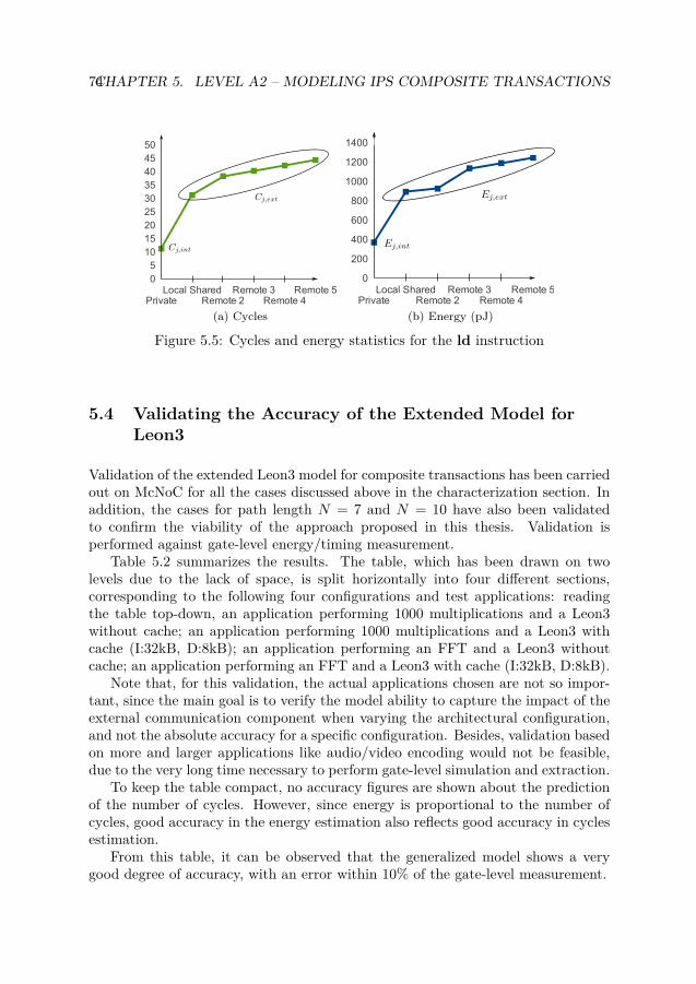
74CHAPTER 5. LEVEL A2 – MODELING IPS COMPOSITE TRANSACTIONS
PrivateLocal Shared
Remote 2Remote 3
Remote 4Remote 5
05101520253035404550
(a) CyclesPrivate
Local SharedRemote 2
Remote 3Remote 4
Remote 50
200
400
600
800
1000
1200
1400
(b) Energy (pJ)
Figure 5.5: Cycles and energy statistics for the ld instruction
5.4 Validating the Accuracy of the Extended Model forLeon3
Validation of the extended Leon3 model for composite transactions has been carriedout on McNoC for all the cases discussed above in the characterization section. Inaddition, the cases for path length N = 7 and N = 10 have also been validatedto confirm the viability of the approach proposed in this thesis. Validation isperformed against gate-level energy/timing measurement.
Table 5.2 summarizes the results. The table, which has been drawn on twolevels due to the lack of space, is split horizontally into four different sections,corresponding to the following four configurations and test applications: readingthe table top-down, an application performing 1000 multiplications and a Leon3without cache; an application performing 1000 multiplications and a Leon3 withcache (I:32kB, D:8kB); an application performing an FFT and a Leon3 withoutcache; an application performing an FFT and a Leon3 with cache (I:32kB, D:8kB).
Note that, for this validation, the actual applications chosen are not so impor-tant, since the main goal is to verify the model ability to capture the impact of theexternal communication component when varying the architectural configuration,and not the absolute accuracy for a specific configuration. Besides, validation basedon more and larger applications like audio/video encoding would not be feasible,due to the very long time necessary to perform gate-level simulation and extraction.
To keep the table compact, no accuracy figures are shown about the predictionof the number of cycles. However, since energy is proportional to the number ofcycles, good accuracy in the energy estimation also reflects good accuracy in cyclesestimation.
From this table, it can be observed that the generalized model shows a verygood degree of accuracy, with an error within 10% of the gate-level measurement.

5.4. VALIDATING THE ACCURACY OF THE EXTENDED MODEL FORLEON3 75
Table 5.2: Leon3 model validation versus gate-level energy measurement
Private Local shared Path through Path throughmemory memory 2 nodes 3 nodes
1000 multiplications – no cache# Instructions 11513 11513 11513 11513Measured energy (µJ) 3.6738 5.2750 5.8626 6.0232Estimated energy (µJ) 3.6058 5.1948 5.2864 5.9438Error (%) -1.85 -1.52 -9.83 -1.32
1000 multiplications - cache (I:32kB, D:8kB)# Instructions 11513 11513 11513 11513Measured energy (µJ) 0.9664 1.3435 1.5619 1.6162Estimated energy (µJ) 1.0253 1.4064 1.5675 1.7114Error (%) 6.10 4.68 0.36 5.89
FFT - no cache# Instructions 683485 683485 683485 683485Measured energy (mJ) 0.1232 0.1237 0.1238 0.1239Estimated energy (mJ) 0.1267 0.1272 0.1272 0.1273Error (%) 2.83 2.83 2.72 2.82
FFT - cache (I:32kB, D:8kB)# Instructions 683485 683485 683485 683485Measured energy (mJ) 0.0431 0.0434 0.0435 0.0436Estimated energy (mJ) 0.0473 0.0477 0.0479 0.0479Error (%) 9.97 10.00 9.96 10.00
Path through Path through Path through Path through4 nodes 5 nodes 7 nodes 10 nodes
1000 multiplications – no cache# Instructions 11513 11513 11513 11513Measured energy (µJ) 6.1841 6.3430 6.6644 7.1480Estimated energy (µJ) 6.1070 6.2638 6.5848 7.0648Error (%) -1.25 -1.25 -1.19 -1.16
1000 multiplications - cache (I:32kB, D:8kB)# Instructions 11513 11513 11513 11513Measured energy (µJ) 1.6713 1.7250 1.8344 1.9998Estimated energy (µJ) 1.7399 1.7915 1.9016 2.0653Error (%) 4.11 3.86 3.66 3.27
FFT - no cache# Instructions 683485 683485 683485 683485Measured energy (mJ) 0.1239 0.1239 0.1240 0.1241Estimated energy (mJ) 0.1274 0.1274 0.1275 0.1276Error (%) 2.82 2.82 2.82 2.81
FFT - cache (I:32kB, D:8kB)# Instructions 683485 683485 683485 683485Measured energy (mJ) 0.0436 0.0437 0.0437 0.0439Estimated energy (mJ) 0.0480 0.0480 0.0481 0.0482Error (%) 10.00 10.00 10.00 9.99

76CHAPTER 5. LEVEL A2 – MODELING IPS COMPOSITE TRANSACTIONS
5.5 Summary
This chapter has presented a method aimed at modeling composite transactionswhen building IP energy and performance models. This is done with the intent ofmaintaining accurate models regardless of the platform used. A Leon3 processorhas been taken as a reference IP, while a System on Chip and a Network on Chiphave been taken as reference platforms. After discussing the method, the resultingIP model has also been validated for energy estimation accuracy. The results haveshown it to be within 10% of gate-level estimation.

Chapter 6
Level B – Inferring PrimaryTransactions and Refinements forTransactions Interdependency andCaches
This chapter applies the steps described in Section 3.4 about inferring primary trans-actions at the Algorithmic Level. At the same time, it also discusses a refinementrelated to transactions interdependency and caches. Inference of primary transac-tions is done for a set of common benchmark applications. Energy and performancenumbers for these applications are then estimated by Funtime and compared againstgate-level extraction. The Funtime estimation speed is instead compared againstTransaction-Level Modeling. It is found out that Funtime estimation accuracy iswithin 15% of the gate-level estimation and that Funtime is about 30X faster thanthe corresponding TLM implementation. The material presented in this chapter isbased on the author’s publication in [61].
6.1 Introduction
As discussed in Section 3.4, the Algorithmic Level (Level B) is Funtime’s mainestimation level and is the end-user’s entry point for using the Funtime framework.By relying on the availability of an applications database B, of an ArchitectureSpecification (AS) and of a Use-Case Specification (UCS), the Algorithmic Levelinfers a trace of transactions (primary transactions) for individual applications.These traces are then passed up to the Refinement Level (Level C), which appliesa set of refinements to them (secondary transactions) and enables accurate energyand performance estimation. For better clarity, a diagram of the Algorithmic Levelis reported in Figure 6.1.
The figure shows that instrumentation is the first step performed at Level B.
77
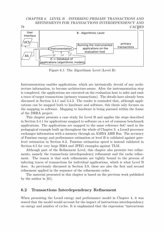
78
CHAPTER 6. LEVEL B – INFERRING PRIMARY TRANSACTIONS ANDREFINEMENTS FOR TRANSACTIONS INTERDEPENDENCY AND
CACHES
InstrumentationRunning the instrumented
applications on the evaluation host
B - Algorithmic Level
primarytransactions
UCS
AS
UserInterface
:= Database of applications (algorithmic models)
Figure 6.1: The Algorithmic Level (Level B)
Instrumentation enables applications, which are intrinsically devoid of any archi-tecture information, to become architecture-aware. After the instrumentation stepis completed, the applications are executed on the evaluation host to infer and emita trace of target transactions (primary transactions). The details have already beendiscussed in Section 3.4.1 and 3.4.2. The reader is reminded that, although appli-cations can be mapped both to hardware and software, this thesis only focuses onthe mapping to software. Mapping to hardware is being pursued within the frameof the DRRA project.
This chapter presents a case study for Level B and applies the steps describedin Section 3.4.1 for applications mapped to software on a set of common benchmarkapplications. The applications are mapped to the same reference SoC used in thepedagogical example built up throughout the whole of Chapter 3: a Leon3 processorexchanges information with a memory through an AMBA AHB Bus. The accuracyof Funtime energy and performance estimation at level B is validated against gate-level estimation in Section 6.3. Funtime estimation speed is instead validated inSection 6.5 for very large H264 and JPEG examples against TLM.
Although part of the Refinement Level, this chapter also presents two refine-ments, namely the transactions interdependency refinement and the cache refine-ment. The reason is that such refinements are tightly bound to the process ofinferring traces of transactions for individual applications, which is what Level Bdoes. As previously discussed in Section 3.9, these are also the first and secondrefinement applied in the sequence of the refinements order.
The material presented in this chapter is based on the previous work publishedby the author in [61].
6.2 Transactions Interdependency Refinement
When presenting the Leon3 energy and performance model in Chapter 4, it wasstated that the model would account for the impact of instructions interdependencyon energy and number of cycles. It is emphasized that the expression “instructions
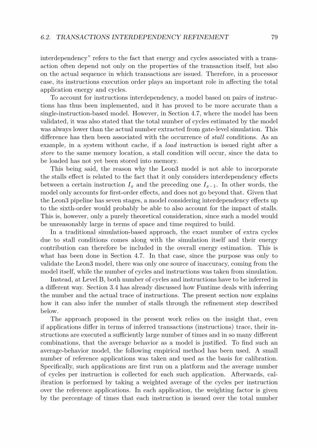
6.2. TRANSACTIONS INTERDEPENDENCY REFINEMENT 79
interdependency” refers to the fact that energy and cycles associated with a trans-action often depend not only on the properties of the transaction itself, but alsoon the actual sequence in which transactions are issued. Therefore, in a processorcase, its instructions execution order plays an important role in affecting the totalapplication energy and cycles.
To account for instructions interdependency, a model based on pairs of instruc-tions has thus been implemented, and it has proved to be more accurate than asingle-instruction-based model. However, in Section 4.7, where the model has beenvalidated, it was also stated that the total number of cycles estimated by the modelwas always lower than the actual number extracted from gate-level simulation. Thisdifference has then been associated with the occurrence of stall conditions. As anexample, in a system without cache, if a load instruction is issued right after astore to the same memory location, a stall condition will occur, since the data tobe loaded has not yet been stored into memory.
This being said, the reason why the Leon3 model is not able to incorporatethe stalls effect is related to the fact that it only considers interdependency effectsbetween a certain instruction Ix and the preceding one Ix−1. In other words, themodel only accounts for first-order effects, and does not go beyond that. Given thatthe Leon3 pipeline has seven stages, a model considering interdependency effects upto the sixth-order would probably be able to also account for the impact of stalls.This is, however, only a purely theoretical consideration, since such a model wouldbe unreasonably large in terms of space and time required to build.
In a traditional simulation-based approach, the exact number of extra cyclesdue to stall conditions comes along with the simulation itself and their energycontribution can therefore be included in the overall energy estimation. This iswhat has been done in Section 4.7. In that case, since the purpose was only tovalidate the Leon3 model, there was only one source of inaccuracy, coming from themodel itself, while the number of cycles and instructions was taken from simulation.
Instead, at Level B, both number of cycles and instructions have to be inferred ina different way. Section 3.4 has already discussed how Funtime deals with inferringthe number and the actual trace of instructions. The present section now explainshow it can also infer the number of stalls through the refinement step describedbelow.
The approach proposed in the present work relies on the insight that, evenif applications differ in terms of inferred transactions (instructions) trace, their in-structions are executed a sufficiently large number of times and in so many differentcombinations, that the average behavior as a model is justified. To find such anaverage-behavior model, the following empirical method has been used. A smallnumber of reference applications was taken and used as the basis for calibration.Specifically, such applications are first run on a platform and the average numberof cycles per instruction is collected for each such application. Afterwards, cal-ibration is performed by taking a weighted average of the cycles per instructionover the reference applications. In each application, the weighting factor is givenby the percentage of times that each instruction is issued over the total number

80
CHAPTER 6. LEVEL B – INFERRING PRIMARY TRANSACTIONS ANDREFINEMENTS FOR TRANSACTIONS INTERDEPENDENCY AND
CACHESof instructions. The resulting numbers are then taken as a model and applied tonew applications to estimate the total applications length in terms of cycles. Thedifference between the total application cycles found by using the refined valuesand the total application cycles found by using the ideal values given by the pro-cessor model represents the contribution of the stalls and, consequently, the effectof transactions interdependency.
The assumption about the possibility of finding typical patterns across differ-ent applications relies on the fact that predictability is usually strongly desired inembedded systems, and especially in those systems that have to fullfill real-time con-straints. In addition, applications often consist of large loops which are identicallyrepeated a large number of times. This further helps to support this assumption.To achieve the highest possible accuracy, applications may be grouped accordingto the main functionality that they implement and calibration can then be doneon each individual group. For example, video, audio and image encoding/decodingapplications could represent individual groups.
Since in Section 4.7 the quantity Estall
cycle has been defined as the stall energyper cycle, it now makes sense to associate the duration of a single stall to onecycle. Under these assumptions, the total number of stalls can be expressed as inEquation 6.1:
#Stalls = Tot_estimated_cycles− Tot_ideal_cycles (6.1)Similarly, the total energy contribution due to the stalls can be calculated as inEq. 6.2.
Estalls = #Stalls · Estallcycle
(6.2)
In the context of the research presented in this thesis, the transactions interde-pendency refinement has been applied to a SoC based on a Leon3 processor thatexchanges information with a memory through an AMBA AHB bus. The Leon3processor has been configured with no cache to avoid the introduction of extrasources of indeterminism. A set of three different applications has been taken as areference and used for calibration, namely an FFT, a Quicksort and a Fibonacci se-ries. Table 6.1 shows a comparison between the ideal processor cycles when a cachehit occurs and the refined ones for a bunch of Leon3 instructions. The transactionsinterdependency refinement applied to the Algorithmic Level has been validated inSection 6.3.
6.3 Validating the Algorithmic Level and the Accuracy ofthe Transactions Interdependency Refinement
Gate level has been used as a reference for validation, since it is very accurate andhas been used to build the Leon3 energy and performance model. The results arereported in Tables 6.2 and 6.3. These tables validate the accuracy of the Algorith-mic Level plus the transactions interdependency refinement for seven benchmarks

6.3. VALIDATING THE ALGORITHMIC LEVEL AND THE ACCURACY OFTHE TRANSACTIONS INTERDEPENDENCY REFINEMENT 81
Table 6.1: Comparison between ideal and real average cycles per instruction
Instr. Ideal cycles Real avg. cyclesadd 1.00 7.58ld 1.00 15.19nop 1.00 3.23st 2.00 5.82... ... ...
by introducing a growing number of sources of inaccuracy. Note that the threeapplications on the top of each table represent the calibration suite referenced inthe refinement section above, whereas the four applications at the bottom are thevalidation set, not part of the calibration. In both tables, the Leon3 configurationwithout cache has been selected.
Table 6.2 introduces two sources of inaccuracy: the first refers to the trans-actions interdependency refinement used to estimate the total number of cycles(ideal + stalls contribution); the second refers to the Leon3 energy and perfor-mance model. The number of actual instructions is measured. Table 6.3 introducesinstead three sources of inaccuracy: the first two are the same as in Table 6.2,while the third refers to the number of transactions (instructions) estimated by theAlgorithmic Level. Even in this case, the maximum error of Funtime for energyestimation is around 15% of the gate level.
Table 6.2: 2 sources of inaccuracy: Leon3 energy & performance model + estimatednumber of cycles (stalls)
Calibration benchmarksFFT Quicksort Fibonacci
# Instructions 1 371 584 4 008 651 1 585 313Real # cycles 6 485 094 31 649 232 13 902 019Estimated # cycles 7 217 187 31 153 927 13 251 730Error [%] +11.29 -1.56 -4.68Real energy [mJ] 0.2396 1.1508 0.4906Estimated energy [mJ] 0.2746 1.0719 0.4509Error [%] +14.62 -6.86 -8.10
Verification benchmarksViterbi Queens Dhrystone MD5
# Instructions 2 452 903 4 266 783 1 950 813 1 802 380Real # cycles 17 511 989 24 193 885 15 938 144 14 428 588Estimated # cycles 18 484 266 24 878 824 15 660 388 14 082 568Error [%] +5.55 +2.83 -1.74 -2.40Real energy [mJ] 0.6250 0.8571 0.5641 0.5228Estimated energy [mJ] 0.6648 0.9013 0.5498 0.4989Error [%] +6.36 +5.15 -2.54 -4.74

82
CHAPTER 6. LEVEL B – INFERRING PRIMARY TRANSACTIONS ANDREFINEMENTS FOR TRANSACTIONS INTERDEPENDENCY AND
CACHESTable 6.3: 3 sources of inaccuracy: Leon3 energy & performance model + estimatednumber of cycles (stalls) + estimated number of instructions
Calibration benchmarksFFT Quicksort Fibonacci
Real # instructions 1 371 584 4 008 651 1 585 313Estimated # instructions 1 273 927 3 824 253 1 517 196Error [%] -7.12 -4.6 -4.3Real # cycles 6 485 094 31 649 232 13 902 019Estimated # cycles 6 731 528 29 427 456 12 185 120Error [%] +3.8 -7.02 -12.35Real energy [mJ] 0.2396 1.1508 0.4906Estimated energy [mJ] 0.2666 1.0417 0.4061Error [%] +11.29 -9.48 -17.23
Verification benchmarksViterbi Queens Dhrystone MD5
Real # instructions 2 452 903 4 266 783 1 950 813 1 802 380Estimated # instructions 2 398 390 4 006 083 1 880 389 1 707 214Error [%] -2.22 -6.11 -3.61 -5.28Real # cycles 17 511 989 24 193 885 15 938 144 14 428 588Estimated # cycles 17 783 529 23 680 975 15 131 674 13 233 901Error [%] +3.55 -2.12 -5.06 -8.28Real energy [mJ] 0.6250 0.8571 0.5641 0.5228Estimated energy [mJ] 0.6611 0.9054 0.5265 0.4588Error [%] +5.78 +5.64 -6.67 -12.25
6.4 Cache Effect Refinement
The presence of caches is an additional factor that affects the estimation accuracyat the Level B of the Funtime approach. The refinement applied in this case aimsat quantifying and modeling the variation of an application execution time andenergy in a system with cache, given the cache miss ratio MR and compared tothe case with no cache. The cache miss ratio must thus be provided as an inputto Funtime, in the UCS. As opposed to the effect of transactions interdependency,caches reduce the total amount of application cycles, since there are fewer stallscaused by communication with memory.
Also in this case, the way in which the refinement is implemented relies on theassumption that the percentage of cycles variation for a given cache miss ratio,compared to the case without cache, is independent from the application and usecase for an application. This assumption is again justified by the fact that anaverage behavior can be modeled using a calibration set as shown in Figure 6.2, as aconsequence of the large number of instructions and instruction sequences generatedby each application. Similarly to the previous refinement, a small set of applicationscan therefore be taken as the basis for calibration and the results of calibration canthen be applied to refine new applications, which form the validation suite as shownin Figure 6.2. Calibration in this case consists in finding an interpolation function.
The same calibration benchmarks and SoC have been used as for the trans-

6.5. COMPARING FUNTIME AND UNTIMED TLM ESTIMATION SPEED83
actions interdependency refinement. A Leon3 has been configured with a 1k, 2k,4k I/D cache. The interpolation function results in this case in a straight line,expressed in Equation 6.3:
C% = 1.09 ·MR% + 19.19 (6.3)
where C% represents the percentage of total application cycles compared to the casewithout cache andMR% the miss ratio in percentage. Note that, for an ideal case ofMR% = 0%, an application would complete in about 20% of the time with respectto the case with no cache. For the opposite case of MR% = 100%, the equationcannot be applied though, as C% > 100%. It is expected that, starting from acertain point, the function should grow with a smaller slope, so that C% = 100%when MR% = 100%. The experiments conducted in this work only consider anMR% up to 25%, value for which the equation still applies.
Validation for the cache refinement is presented in Figure 6.2. In this case,Equation 6.3, found as an interpolation for the calibration benchmarks, has alsobeen used to estimate the cycles variation also for the other four benchmarks onthe right when using a Leon3 with 1k, 2k, 4k I/D cache. Figure 6.3 shows both theinterpolation straight line extracted from the calibration benchmarks (dashed line)and the real interpolation straight line for the other four applications (thick line).The small difference between the two proves that using Equation 6.3 as a referencefor all the applications is sensible and the error introduced is minimal.
Validation benchmarks
Figure 6.2: Validating the cache refinement
6.5 Comparing Funtime and Untimed TLM EstimationSpeed
For speed comparison, untimed TLM has been chosen as a reference. The reasonis that this represents the fastest high-level methodology for system-level estima-tion commonly used at present. For this purpose, a dedicated transaction-levelmodel in SystemC has been implemented for the reference SoC architecture. The
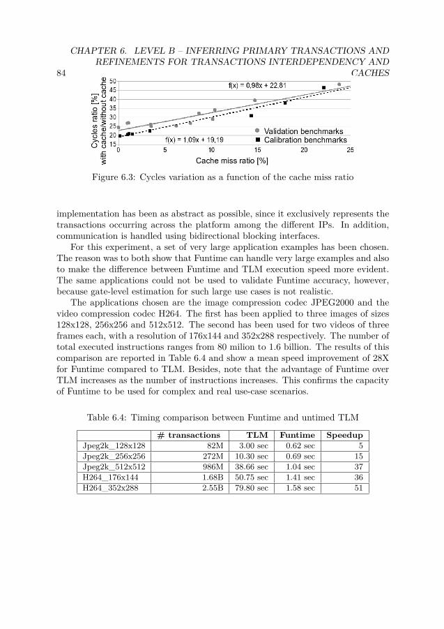
84
CHAPTER 6. LEVEL B – INFERRING PRIMARY TRANSACTIONS ANDREFINEMENTS FOR TRANSACTIONS INTERDEPENDENCY AND
CACHES
Figure 6.3: Cycles variation as a function of the cache miss ratio
implementation has been as abstract as possible, since it exclusively represents thetransactions occurring across the platform among the different IPs. In addition,communication is handled using bidirectional blocking interfaces.
For this experiment, a set of very large application examples has been chosen.The reason was to both show that Funtime can handle very large examples and alsoto make the difference between Funtime and TLM execution speed more evident.The same applications could not be used to validate Funtime accuracy, however,because gate-level estimation for such large use cases is not realistic.
The applications chosen are the image compression codec JPEG2000 and thevideo compression codec H264. The first has been applied to three images of sizes128x128, 256x256 and 512x512. The second has been used for two videos of threeframes each, with a resolution of 176x144 and 352x288 respectively. The number oftotal executed instructions ranges from 80 milion to 1.6 billion. The results of thiscomparison are reported in Table 6.4 and show a mean speed improvement of 28Xfor Funtime compared to TLM. Besides, note that the advantage of Funtime overTLM increases as the number of instructions increases. This confirms the capacityof Funtime to be used for complex and real use-case scenarios.
Table 6.4: Timing comparison between Funtime and untimed TLM
# transactions TLM Funtime SpeedupJpeg2k_128x128 82M 3.00 sec 0.62 sec 5Jpeg2k_256x256 272M 10.30 sec 0.69 sec 15Jpeg2k_512x512 986M 38.66 sec 1.04 sec 37H264_176x144 1.68B 50.75 sec 1.41 sec 36H264_352x288 2.55B 79.80 sec 1.58 sec 51

Chapter 7
Level C – Refining Bus ContentionEffects on Energy and Performance
At Level C, Funtime refines the traces of primary transactions, emitted by LevelB for individual applications, by combining them with a new trace of secondarytransactions. As opposed to Level B, which considers applications in isolation, thisrefinement process basically accounts for the implications of applications having toshare common resources. This chapter shows the case study of an MPSoC, whereapplications mapped to different processors have to share the same bus. A high-level method is proposed for rapidly and accurately predicting the effects of buscontention on energy and performance. The approach consists of two parts: first,a one-time activity performed at Level A2, aimed at identifying and characterizingthe main factors involved in bus contention; second, the development of a predictionmechanism, performed at Level C, to account for the occurrence of such factors foran arbitrary number of processors hosting arbitrary applications. The approach isalso validated against gate-level estimation, and finds out an error within 2%. Thematerial presented in this chapter is based on the previous work published by theauthor in [59].
7.1 Introduction
The ideal scenario has been considered so far where applications are independentand have all the system resources available to themselves. At the Level B, tracesof primary transactions are emitted, which reflect the functionality of applicationstreated in isolation. Nevertheless, in reality there are some implications due to thefact that applications do not have all the resources always available to themselvesand often they even have to interact with other applications. The most visibleeffect of these non-idealities is a variation of the total application execution timeand final energy consumption.
Accounting for the impact of such non-idealities is done in Funtime at the Level
85

86CHAPTER 7. LEVEL C – REFINING BUS CONTENTION EFFECTS ON
ENERGY AND PERFORMANCE
C, also called Refinement Level. At this level, the trace of primary transactionsreceived from Level B is refined through the injection of secondary transactions.The combination of primary and secondary transactions represents the final tracefor which total energy and execution time can be estimated. Estimation is madepossible through the IP energy and performance models, extended at Level A2 andalso passed as an input to Level C.
C - Refinement LevelRefinements- Transactions interdependency- Hw/sw optimizations (caches, etc.)- Operating System - Bus arbitration
primary+
secondary transactions
Output
xUCS
AS
UserInterface
Energy
Exec. time
exte
nded
IP m
odels
pri
mary
tr
ansa
ctio
ns
A2 - Architecture of IPs
Characterizing bus contention
Predicting bus contention
Figure 7.1: The Refinement Level (Level C) - Refining bus contention
Multi-Processor Systems on Chip (MPSoCs) have emerged as one possible so-lution to cope with the demand of increasing performance and computational ef-ficiency in modern embedded architectures. The performance advantage derivesfrom running applications in parallel by distributing them across multiple compu-tational resources, such as processors. In an MPSoC, all the processors are typicallyconnected to the same bus and contention occurs when more than one application,mapped to a certain processor, requests an exclusive access to a shared resource.The main consequence of contention is an overall degradation in performance andan increase in energy consumption.
Refining the effects of bus contention for an MPSoC case study is the purpose ofthis chapter. A high-level method is proposed for rapidly and accurately predictingthe effects of bus contention on energy and performance. The content of this chapteris based on the author’s previous work in [59]. In particular, the bus contentionrefinement is implemented through the following two steps:
1. Characterizing bus contention: this step, which is part of Level A2 and sym-bolically shown at the bottom of Figure 7.1, consists in identifying and charac-
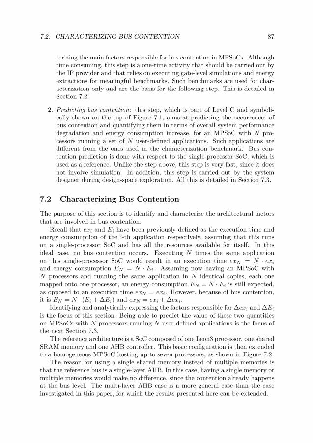
7.2. CHARACTERIZING BUS CONTENTION 87
terizing the main factors responsible for bus contention in MPSoCs. Althoughtime consuming, this step is a one-time activity that should be carried out bythe IP provider and that relies on executing gate-level simulations and energyextractions for meaningful benchmarks. Such benchmarks are used for char-acterization only and are the basis for the following step. This is detailed inSection 7.2.
2. Predicting bus contention: this step, which is part of Level C and symboli-cally shown on the top of Figure 7.1, aims at predicting the occurrences ofbus contention and quantifying them in terms of overall system performancedegradation and energy consumption increase, for an MPSoC with N pro-cessors running a set of N user-defined applications. Such applications aredifferent from the ones used in the characterization benchmark. Bus con-tention prediction is done with respect to the single-processor SoC, which isused as a reference. Unlike the step above, this step is very fast, since it doesnot involve simulation. In addition, this step is carried out by the systemdesigner during design-space exploration. All this is detailed in Section 7.3.
7.2 Characterizing Bus Contention
The purpose of this section is to identify and characterize the architectural factorsthat are involved in bus contention.
Recall that exi and Ei have been previously defined as the execution time andenergy consumption of the i-th application respectively, assuming that this runson a single-processor SoC and has all the resources available for itself. In thisideal case, no bus contention occurs. Executing N times the same applicationon this single-processor SoC would result in an execution time exN = N · exiand energy consumption EN = N · Ei. Assuming now having an MPSoC withN processors and running the same application in N identical copies, each onemapped onto one processor, an energy consumption EN = N · Ei is still expected,as opposed to an execution time exN = exi. However, because of bus contention,it is EN = N · (Ei + ∆Ei) and exN = exi + ∆exi.
Identifying and analytically expressing the factors responsible for ∆exi and ∆Eiis the focus of this section. Being able to predict the value of these two quantitieson MPSoCs with N processors running N user-defined applications is the focus ofthe next Section 7.3.
The reference architecture is a SoC composed of one Leon3 processor, one sharedSRAM memory and one AHB controller. This basic configuration is then extendedto a homogeneous MPSoC hosting up to seven processors, as shown in Figure 7.2.
The reason for using a single shared memory instead of multiple memories isthat the reference bus is a single-layer AHB. In this case, having a single memory ormultiple memories would make no difference, since the contention already happensat the bus level. The multi-layer AHB case is a more general case than the caseinvestigated in this paper, for which the results presented here can be extended.
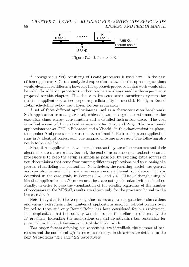
88CHAPTER 7. LEVEL C – REFINING BUS CONTENTION EFFECTS ON
ENERGY AND PERFORMANCE
(Leon3)AHB Ctrl
M(SRAM)
P1(Leon3)
P7......
(Round Robin)
Figure 7.2: Reference SoC
A homogeneous SoC consisting of Leon3 processors is used here. In the caseof heterogeneous SoC, the analytical expressions shown in the upcoming sectionswould clearly look different; however, the approach proposed in this work would stillbe valid. In addition, processors without cache are always used in the experimentsproposed for this chapter. This choice makes sense when considering systems forreal-time applications, whose response predictability is essential. Finally, a RoundRobin scheduling policy was chosen for bus arbitration.
A set of three different applications is used as a characterization benchmark.Such applications run at gate level, which allows us to get accurate numbers forexecution time, energy consumption and a detailed instruction trace. The goalis to find meaningful analytical expressions for ∆exi and ∆Ei. The benchmarkapplications are an FFT, a Fibonacci and a Viterbi. In this characterization phase,the numberN of processors is varied between 1 and 7. Besides, the same applicationruns in N identical copies, each one mapped onto one processor. The following alsoneeds to be clarified.
First, these applications have been chosen as they are of common use and theiralgorithms are quite regular. Second, the goal of using the same application on allprocessors is to keep the setup as simple as possible, by avoiding extra sources ofnon-determinism that come from running different applications and thus easing theprocess of modeling bus contention. Nonetheless, the resulting models are generaland can also be used when each processor runs a different application. This isdescribed in the case study in Sections 7.3.1 and 7.4. Third, although using Nidentical applications on N processors, these are not synchronized with each other.Finally, in order to ease the visualization of the results, regardless of the numberof processors in the MPSoC, results are shown only for the processor bound to thebus at index 0.
Note that, due to the very long time necessary to run gate-level simulationsand energy extractions, the number of applications used for calibration has beenlimited to three and only Round Robin has been considered for bus arbitration.It is emphasized that this activity would be a one-time effort carried out by theIP provider. Extending the applications set and investigating bus contention forpriority-based bus arbitration is part of the future work.
Two major factors affecting bus contention are identified: the number of pro-cessors and the number of w/r accesses to memory. Both factors are detailed in thenext Subsections 7.2.1 and 7.2.2 respectively.
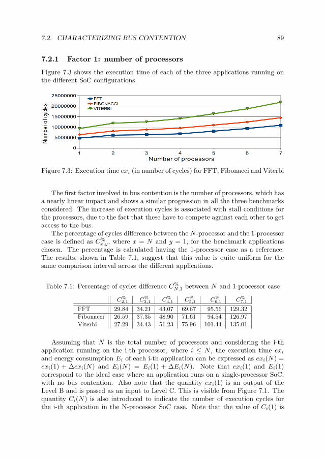
7.2. CHARACTERIZING BUS CONTENTION 89
7.2.1 Factor 1: number of processorsFigure 7.3 shows the execution time of each of the three applications running onthe different SoC configurations.
Figure 7.3: Execution time exi (in number of cycles) for FFT, Fibonacci and Viterbi
The first factor involved in bus contention is the number of processors, which hasa nearly linear impact and shows a similar progression in all the three benchmarksconsidered. The increase of execution cycles is associated with stall conditions forthe processors, due to the fact that these have to compete against each other to getaccess to the bus.
The percentage of cycles difference between the N -processor and the 1-processorcase is defined as C%
x,y, where x = N and y = 1, for the benchmark applicationschosen. The percentage is calculated having the 1-processor case as a reference.The results, shown in Table 7.1, suggest that this value is quite uniform for thesame comparison interval across the different applications.
Table 7.1: Percentage of cycles difference C%N,1 between N and 1-processor case
C%2,1 C%
3,1 C%4,1 C%
5,1 C%6,1 C%
7,1
FFT 29.84 34.21 43.07 69.67 95.56 129.32Fibonacci 26.59 37.35 48.90 71.61 94.54 126.97Viterbi 27.29 34.43 51.23 75.96 101.44 135.01
Assuming that N is the total number of processors and considering the i-thapplication running on the i-th processor, where i ≤ N , the execution time exiand energy consumption Ei of each i-th application can be expressed as exi(N) =exi(1) + ∆exi(N) and Ei(N) = Ei(1) + ∆Ei(N). Note that exi(1) and Ei(1)correspond to the ideal case where an application runs on a single-processor SoC,with no bus contention. Also note that the quantity exi(1) is an output of theLevel B and is passed as an input to Level C. This is visible from Figure 7.1. Thequantity Ci(N) is also introduced to indicate the number of execution cycles forthe i-th application in the N-processor SoC case. Note that the value of Ci(1) is
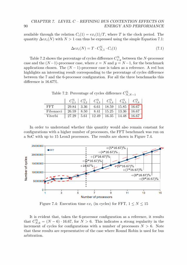
90CHAPTER 7. LEVEL C – REFINING BUS CONTENTION EFFECTS ON
ENERGY AND PERFORMANCE
available through the relation Ci(1) = exi(1)/T , where T is the clock period. Thequantity ∆exi(N) with N > 1 can thus be expressed using the simple Equation 7.1:
∆exi(N) = T · C%N,1 · Ci(1) (7.1)
Table 7.2 shows the percentage of cycles difference C%x,y between theN -processor
case and the (N−1)-processor case, where x = N and y = N−1, for the benchmarkapplications chosen. The (N − 1)-processor case is taken as a reference. A red boxhighlights an interesting result corresponding to the percentage of cycles differencebetween the 7 and the 6-processor configuration. For all the three benchmarks thisdifference is 16.67%.
Table 7.2: Percentage of cycles difference C%N,N−1
In order to understand whether this quantity would also remain constant forconfigurations with a higher number of processors, the FFT benchmark was run ona SoC with up to 15 Leon3 processors. The results are shown in Figure 7.4.
Figure 7.4: Execution time exi (in cycles) for FFT, 1 ≤ N ≤ 15
It is evident that, taken the 6-processor configuration as a reference, it resultsthat C%
N,6 = (N − 6) · 16.67, for N > 6. This indicates a strong regularity in theincrement of cycles for configurations with a number of processors N > 6. Notethat these results are representative of the case where Round Robin is used for busarbitration.

7.2. CHARACTERIZING BUS CONTENTION 91
Three regions are identified in Figure 7.4, highlighted by dashed circles. Thecircle in the middle shows an almost constant number of cycles for the SoC config-urations with 2, 3 and 4 processors. In this case the bus controller allocates to eachprocessor requesting the bus a time slot with the width of a bus transfer. In thecase of a 4-processor SoC, each processor will thus be granted a bus access everyfourth bus transfer. It appears that this time frame is short enough to allow aprocessor to continue its execution without stalling until it regains control over thebus. That is why the performance penalty introduced is insignificant.
However, for configurations with more than 4 processors, this time frame be-comes too long and the processor has to stall for some time before it can access thebus again and continue its execution. This leads to the behavior highlighted by thecircle on the right and to the 16.67% time penalty for any extra processor.
Finally, the circle on the left highlights an execution time difference between theconfigurations with 1 and 2 processors, which apparently contradicts the interpre-tation given above for the configurations with 2 to 4 processors. The explanation isfound in the way the bus controller operates: if there is only one master requestingthe bus, no arbitration is done and thus no arbitration penalty is introduced.
The energy difference has also been measured for the same benchmark applica-tions on the 7 SoC configurations, which results in a linear energy increase propor-tional to the processors number. The increase in energy consumption is a directconsequence of the increased execution time, which has been previously attributedto stall conditions for a processor. Indirectly, it can thus be stated that the energydifference Ei(N) − Ei(1), with N > 1, is also due to stall conditions. In particu-lar, assuming that Estall
cycle is the stall energy overhead per clock cycle, the followingEquation 7.2 can be written:
Estallcycle
= Ei(N)− Ei(1)Ci(N)− Ci(1) (7.2)
The quantity Estall
cycle is expected to be a constant value. Table 7.3 below reportsthe value of Estall
cycle calculated by applying Equation 7.2 to every SoC configurationwith 2 ≤ N ≤ 7 and running the above-mentioned three reference benchmarks. Theconsistency of the results confirms the predictability of the stall energy consumptionper clock cycle, which has an average value Estall
cycle = 24.85 pJ .Note that the value of Estall
cycle reported in this chapter differs from the one cal-culated in Chapter 4 when presenting the Leon3 energy and performance model.This difference can be justified by the difficulty of isolating the exact contributionof each single instruction when building the Leon3 model, and thus by the riskof including extra contributions. Therefore, applying Equation 4.8 to every suchinstruction has not always produced the same result. The average value has thenbeen taken and reported as the reference Estall
cycle value in Chapter 4.With this in mind, the goal is to analytically express the energy overhead
∆Ei(N) for the i-th application as a function of the number of processors N . Thisquantity was previously defined as the extra energy consumed by the i-th applica-

92CHAPTER 7. LEVEL C – REFINING BUS CONTENTION EFFECTS ON
ENERGY AND PERFORMANCE
Table 7.3: Value of Estall
cycle [pJ ] calculated by Equation 7.2 for 2 ≤ N ≤ 7
tion because of bus contention, which is as a function of the number of processorsN . The relation is shown in Equation 7.3.
∆Ei(N) = Estallcycle
· ∆exi(N)T
(7.3)
7.2.2 Factor 2: number of w/r accesses to memoryBesides the number of processors, investigation is also conducted on the impactthat w/r memory accesses have on bus contention compared to instruction fetching.Recall that the reference SoC is composed of processors without cache.
Using the FFT as a reference, the instruction-level difference C%7,1 is measured
in the execution cycles between the 7-processor and the single-processor SoC. Ar-chitectures with such a high different number of processors are compared in orderto make the differences more tangible. Table 7.4 shows the results.
Table 7.4: Percentage of instruction-level cycles difference C%7,1 for the FFT
Table 7.4 consists of two columns, each of which contains three sub-columns.From left to right, these sub-columns show the name of the instruction, its occur-rence compared to the other instructions, and the percentage of execution cyclesdifference C%
7,1. The items are sorted according to increasing values of C%7,1. Clearly,
for all instructions the value of C%7,1 is positive. This makes sense, since processors

7.2. CHARACTERIZING BUS CONTENTION 93
without cache are being used, which implies that all instructions need to be fetcheddirectly from memory. Contention can therefore happen for any instruction.
The reader is reminded that the purpose of this analysis is to see whetherthe value of C%
7,1, for instructions related to store/load operations, is above theaverage compared to the rest of the instructions. If this is the case, consideringthe load/store-related instructions as a second factor in modeling bus contentioncan be useful to improve the estimation accuracy. In our example, the averagevalue of C%
7,1 is 129.32%, when measured on an application-level basis. A dashedline has been used as a separator between those instructions whose C%
7,1 is belowand above average respectively. Red boxes have then been used to highlight all theload/store-related instructions. Not surprisingly, all such instructions show a valuefor C%
7,1 above average. In fact, in this case, not only fetching represents a possibilityfor contention, but also writing/reading data to/from memory. Nonetheless, thereare also some non-store/load-related instructions exhibiting execution time aboveaverage. Some of them operate on data, however, – such as add, sll and sub – anda delay can be introduced if the data is not available when the instruction is issued.
Although the occurrence of load/store-related instructions is lower than 12% ofthe total in the FFT case, this value rises to ∼27% in the Fibonacci and Viterbicases. Thus, it seems that explicitly considering the load/store-related instructionsas a second factor in modeling bus contention can improve the estimation accu-racy for ∆exi. This can be done by separately considering the contribution of theload/store-related instructions and the non-store/load-related ones. If the formerand latter group of instructions are denoted by the symbol wr and wr respectively,Equation 7.1 can be reformulated as Equation 7.4:
∆exi(N,wr) = T · [C%wr,N,1 · Ci,wr(1) + C%
wr,N,1 · Ci,wr(1)] (7.4)
Note that the methodology presented above will be generalized in the nextsections and applied to the case study in Section 7.3.1.
7.2.3 SummaryThe key concepts introduced so far can be summarized as follows:
1) The symbols exi(1) and Ei(1) refer to the execution time and energy con-sumption of the i-th application for the single-processor case, where no contentionoccurs. These are also the quantities produced by the Level B of Funtime.
2) The execution time variation ∆exi(N) and energy variation ∆Ei(N) havebeen analytically expressed for the N-processor case with N > 1 compared to thecase where N = 1. See Equations 7.1 and 7.3.
3) Two main factors affecting bus contention have been considered: the numberof processors and the number of w/r accesses to memory. Considering this secondfactor allows the extension of Equation 7.1 into Equation 7.4.
4) Since simulating and extracting energy at gate level is very time-consuming,the analysis has been limited to three examples using configurations with up to

94CHAPTER 7. LEVEL C – REFINING BUS CONTENTION EFFECTS ON
ENERGY AND PERFORMANCE
seven processors. These examples are used for characterization and for the cre-ation of analytical expressions for ∆exi(N) and ∆Ei(N). During validation inSection 7.4, a different set of examples is used to ensure the generality and ac-curacy of these expressions. Only for the FFT application has the analysis beenextended to a SoC with up to 15 processors. This allowed a very regular behaviorto be measured for configurations with more than seven processors. See Figure 7.4.
5) Despite the very long characterization time, this is a one-time activity, whichshould be done by the IP provider. The equations and the quantities extracted inthis section will be the basis for the upcoming bus contention prediction section.
7.3 Predicting Bus Contention
The present section elaborates on how the results from Section 7.2 can be usedand extended to predict the bus contention occurrences on an N -processor SoCrunning N arbitrary applications. It is emphasized that bus contention occurrencesare evaluated in terms of variation in the execution time ∆exi(N,wr) and energyconsumption ∆Ei(N,wr) for each i-th application.
As opposed to the bus contention characterization process, which is a one-timeactivity carried out by the IP provider at Level A2, the bus contention predictionis made at the Level C by the SoC architect during design-space exploration. Inaddition, while the characterization process is time consuming since it relies on adynamic estimation based on gate-level simulation, the prediction activity is veryfast, since it applies well-defined equations, such as Eq. 7.4 and 7.3, on a codeprofiled during execution on the host and back-annotated with target-specific in-formation. The following case study shows how efficient bus contention predictioncan be made.
7.3.1 Case study
This case study is meant to generalize Equation 7.4, so that it can still be appliedto the case of an MPSoC with N processors running N different applications thatcan start and finish at any time.
An MPSoC execution time exmpsoc is defined as the range of time beginningwhen the first of theN processors starts its execution at time ts and ending when thelast processor finishes its execution at time tf . It is therefore true that exmpsoc =max(tf )−min(ts). In addition, for this case study the number of active processorsna can vary in time, until it becomes 0 when the last application has completedits execution. Thus, it is true that 0 ≤ na ≤ N . Since bus contention can only becaused by an active processor trying to access the bus, exi(N,wr) and Ei(N,wr)can be rewritten more precisely as exi(na, wr) and Ei(na, wr). Keeping track of thevariation of na over time is critical. Note also that, when 0 ≤ na ≤ N , there willbe N − na processors in the idle state. This scenario is shown in Figure 7.5, wherefive different applications are considered running on five processors [P1, ..., P5], and

7.3. PREDICTING BUS CONTENTION 95
where each i-th application starts and finishes at different times ts,i and tf,i. Theprocessors in idle state are represented by dotted lines.
Figure 7.5: MPSoC execution time for N processors and N different applications
Using Equation 7.4 derived in the previous Section 7.2, the goal is to predict thevalue exi(na, wr) for any possible application. The only unknown elements in theequation are C%
wr,N,1 and C%wr,N,1, which indicate the percentage of cycles variation
between the N-processor case and the 1-processor case, for instructions respectivelynon-related and related to store/load operations. The approach proposed in thissection is to use the average values C%
wr,N,1 and C%wr,N,1 (see Table 7.5) calculated
on the characterization benchmarks, i.e. FFT, Fibonacci and Viterbi, and applysuch averages to other applications as well for. Section 7.4 proves the generality ofthe model and that the error introduced is minimal. These average values are shownin Table 7.5. Equation 7.4 generalized to any i-th application becomes therefore:
∆exi(na, wr) = T · [C%wr,na,1 · Ci,wr(1) + C%
wr,na,1 · Ci,wr(1)] (7.5)
Table 7.5: Average C%wr,na,1 and C%
wr,na,1 calculated on the FFT, Fibonacci andViterbi benchmarks
C%2,1 C%
3,1 C%4,1 C%
5,1 C%6,1 C%
7,1
wr 27.38 30.87 37.92 59.66 82.76 112.16wr 27.16 48.77 75.56 108.57 141.03 183.43
Since it also consumes energy, the idle state has to be taken into account. Energyconsumption due to an idle state can be expressed as follows:
Ei,idle = Pidle · (exmpsoc − exi) (7.6)
where Pidle is the power consumption of the processor when in idle state. Thecomplete equations for execution time and energy consumption can thus be rewrit-ten as exi(na, wr) = exi(1, wr) + ∆exi(na, wr) and Ei(na, wr) = Ei(1, wr) +∆Ei(na, wr) + Ei,idle respectively.
Note that the starting time ts,i for each i-th application is a user-defined param-eter. Although ignored in the present paper, normally there would be an operating
96CHAPTER 7. LEVEL C – REFINING BUS CONTENTION EFFECTS ON
ENERGY AND PERFORMANCE
system taking care of releasing the different applications (or tasks) according to theuser settings. The value of tf,i is instead calculated by the prediction algorithm,as explained below. The times ts and tf are the only points where the na valueis updated. The reason is that there is no other time when this value can change.The result is a static decomposition of the whole applications set into multiple timewindows wk. In Figure 7.5, six time windows [w1, w6] are identified.
Based on all these considerations, an algorithm can be used for predicting buscontention, where Equations 7.3, 7.5 and 7.6 introduced above are used iterativelyto predict both execution time and energy consumption for each i-th applicationrunning on an N -processor SoC. Note that, since the values are updated only incorrespondence to the beginning/end of a time window, prediction is very fastand its speed is proportional to the number of applications, not to their executionlength. Specifically, the prediction algorithm consists of the following four mainsteps, which are performed whenever a new window wk starts:
1) The value of na is updated.2) The ending time of the time window is identified as the minimum time be-
tween all the tf,i of the applications that are still running and the next closeststarting time ts,i. The value of tf,i is calculated as a function of the na value forthe present window.
3) For each i-th application, the values of ∆exi(na, wr) and ∆Ei(na, wr) areupdated using Equations 7.5 and 7.3.
4) The process iterates until all applications have completed and na = 0. Thevalue of Ei,idle can then also be updated using Equation 7.6, since exmpsoc is known.
7.4 Validating the Accuracy of Bus Contention Prediction
To validate the accuracy of Funtime in estimating bus contention penalty, gate-levelmeasurements are used as a reference. The reason is that gate-level estimation isvery accurate. The reference SoC architecture is the same as that used during thebus contention characterization phase, as reported in Figure 7.2. The 1-processorconfiguration is taken as a reference and measured values exi(1) and Ei(1) are used.
N different applications are considered, which run on N processors. Each i-thapplication is mapped onto only one processor. The case presented here runs ona 3-processor SoC. The three applications, which are different for the ones usedduring the characterization phase, are a Quicksort on P1, a Dhrystone on P2 andthe N-queen problem on P3. Since there is no OS running, all applications start atthe same time, but can finish at different times.
Table 7.6 shows the results for measured versus predicted execution time andenergy. It also shows the number of active processors na and the current state ofeach processor, i.e. active or idle. The predicted values for execution time andenergy are calculated by using the algorithm described in Subsection 7.3.1. It isfound that the prediction error is below 2%. In the energy prediction case, the idleenergy is also considered in the error calculation.

7.5. SUMMARY 97
Table 7.6: Measured vs. predicted execution time exi[ms] and Ei[µJ ]. 3 differentapplications on a 3-processor SoC.
P1 P2 P3na Quicksort Dhrystone Queens
3measured exi
active
active
98.89Ei 145.18
predicted exi 97.69Ei 143.42
2measured exi 248.87
idle
Ei 377.38
predicted exi 248.94Ei 377.51
1measured exi 463.29
idleEi 760.50
predicted exi 463.36Ei 760.65
Error[%] exi +0.01 +0.03 -1.21Ei +0.02 +0.06 -1.23
7.5 Summary
A high-level method has been presented for rapidly and accurately predicting buscontention effects on energy and performance in MPSoCs. The proposed approachconsists of two steps: first, a one-time activity performed at Level A2, aimed atidentifying and characterizing the main factors involved in bus contention; second,the development of a prediction mechanism, performed at Level C, to accountfor the occurrence of such factors for an arbitrary number of processors hostingarbitrary applications. As a result, a high prediction accuracy is achieved, which iswithin ∼2% of the gate-level estimation.


Chapter 8
Level C – Refining the OperatingSystem Overhead on Energy andPerformance
This chapter continues with the description of the Refinement Level. A high-levelmethod is here presented for rapidly and accurately estimating energy and perfor-mance overhead of Real-Time Operating Systems. Two main components are dis-tinguished in the approach: first, an accurate one-time pre-characterization of themain RTOS functionalities in terms of energy and cycles; this activity is performedat Level A1 by the IP provider. Second, the development of an algorithm to rapidlypredict the occurrences of such RTOS functionalities; this activity is performed atLevel C. The approach is also validated against gate-level estimation, obtaining aworst-case error of 12%. The material presented in this chapter is based on theprevious work published by the author in [58] and [57].
8.1 Introduction
The previous chapter has discussed the Refinement Level (Level C) by presenting amethod for predicting the occurrences of bus contention in MPSoCs. The presentchapter continues the description of the Refinement Level by proposing a methodto account for the operating system overhead.
Real-Time Operating Systems (RTOS) are critical infra-structural componentsof embedded SoCs. They enable and manage sharing of hardware resources: com-putational, storage, interconnect and I/O. However, such services have an overhead,both in latency and energy. This overhead needs to be accounted for when doingdesign-space exploration and energy/performance estimation at system level, earlyin the design cycle. Without factoring in this overhead, the accuracy of the esti-mates would be severely compromised.
At the Level B of the Funtime approach, the simplified scenario has been consid-
99
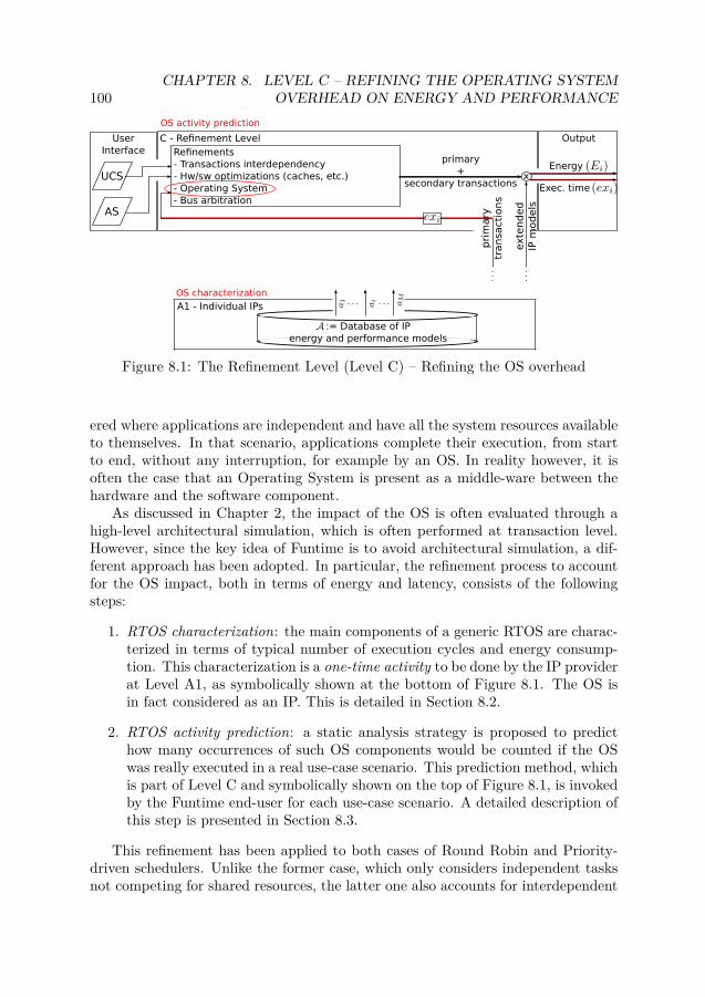
100CHAPTER 8. LEVEL C – REFINING THE OPERATING SYSTEM
OVERHEAD ON ENERGY AND PERFORMANCE
C - Refinement LevelRefinements- Transactions interdependency- Hw/sw optimizations (caches, etc.)- Operating System - Bus arbitration
primary+
secondary transactions
Output
xUCS
AS
UserInterface
Energy
Exec. time
exte
nded
IP m
odels
pri
mary
tr
ansa
ctio
ns
A1 - Individual IPs
:= Database of IP energy and performance models
OS characterization
OS activity prediction
Figure 8.1: The Refinement Level (Level C) – Refining the OS overhead
ered where applications are independent and have all the system resources availableto themselves. In that scenario, applications complete their execution, from startto end, without any interruption, for example by an OS. In reality however, it isoften the case that an Operating System is present as a middle-ware between thehardware and the software component.
As discussed in Chapter 2, the impact of the OS is often evaluated through ahigh-level architectural simulation, which is often performed at transaction level.However, since the key idea of Funtime is to avoid architectural simulation, a dif-ferent approach has been adopted. In particular, the refinement process to accountfor the OS impact, both in terms of energy and latency, consists of the followingsteps:
1. RTOS characterization: the main components of a generic RTOS are charac-terized in terms of typical number of execution cycles and energy consump-tion. This characterization is a one-time activity to be done by the IP providerat Level A1, as symbolically shown at the bottom of Figure 8.1. The OS isin fact considered as an IP. This is detailed in Section 8.2.
2. RTOS activity prediction: a static analysis strategy is proposed to predicthow many occurrences of such OS components would be counted if the OSwas really executed in a real use-case scenario. This prediction method, whichis part of Level C and symbolically shown on the top of Figure 8.1, is invokedby the Funtime end-user for each use-case scenario. A detailed description ofthis step is presented in Section 8.3.
This refinement has been applied to both cases of Round Robin and Priority-driven schedulers. Unlike the former case, which only considers independent tasksnot competing for shared resources, the latter one also accounts for interdependent

8.2. RTOS CHARACTERIZATION 101
tasks that do compete to lock a shared resource. The material presented in thischapter is based on the author’s previous work published in [58] and [57].
8.2 RTOS Characterization
This section proposes a general approach to characterizing the transactions – sec-ondary transactions in this case – due to the RTOS overhead in terms of latencyand energy. RTOS overheads are implied by its components that are called to im-plement the RTOS functionality. Characterization is a one-time activity done bythe RTOS provider. The process consists in simulating the RTOS in a post-layout,back-annotated gate-level netlist of the representative SoC architecture. Althoughtime consuming, this characterization process is justified because it is done onlyonce and the precision gained is important for the accuracy of estimates at high-level. Although this chapter presents the characterization of the RTEMS RTOS [4]for a Leon-based SoC [1], the methods themselves are generic and do not dependon a specific RTOS implementation or SoC architecture.
The characterization process not only considers atomic RTOS calls, as in [11],but also considers coarse-grained RTOS calls like clock tick interrupts and schedulerinvocation. The number and type of atomic RTOS calls involved both in the clocktick interrupt and in the scheduler are OS-dependent. However, thanks to the gen-eral approach that has been adopted, it is easy to specify the sequence of atomic OSroutines that have to be included in the performance and energy characterization.
8.2.1 Characterizing a group of RTOS routinesThe characterization process is explained in five steps using RTEMS for the Leon3-based SoC shown in Figure 8.2.
Leon3
AHB Ctrl
Timer Irq Ctrl
AHB/APBBridge
APB Ctrl
SRAM
Figure 8.2: Leon3-based platform
1. A representative SoC is composed, with essential hardware for hosting anRTOS. An example is given in Figure 8.2. The platform is then synthesized.Synthesis has been carried out in our case for the TSMC-90nm technology.
2. The RTOS and its tasks are compiled and loaded into the system. Fromthe object file, a memory dump of the RTOS and the tasks is also taken. A

102CHAPTER 8. LEVEL C – REFINING THE OPERATING SYSTEM
OVERHEAD ON ENERGY AND PERFORMANCE
fragment of such a dump is shown in Figure 8.3. In the RTEMS case, thiscan be done using the sparc-rtems-objdump command. The dump allowsany routine name to be associated with its memory addresses.
40006944 <rtems_clock_tick>:40006944: 9d e3 bf 98 save %sp, -104, %sp40006948: 40 00 08 09 call 4000896c <_TOD_Tickle_ticks>4000694c: 01 00 00 00 nop 40006950: 11 10 00 71 sethi %hi(0x4001c400), %o040006954: 40 00 16 77 call 4000c330 <_Watchdog_Tickle>
Figure 8.3: Example of an objdump output
3. The system is executed at gate level, with the user-defined tasks, and theRTOS calls are activated a sufficient number of times – around 1000 in ourcase – to make the characterization statistically relevant.
4. As an output of step 3, an execution trace file and a VCD (Value ChangeDump) file are produced from the gate-level simulation. It is required thatthe execution trace file contains both the address of each instruction that hasbeen executed, as well as its time stamp. The VCD file contains instead theswitching activity figures, used by the EDA tools to do power estimation.
5. By using the information in the dump, execution trace, VCD and by providingthe sequence of atomic RTOS routines to be characterized, it is possible toextract the average number of cycles and also the energy for the routinesunder characterization. This last step has been automated by implementingand using a C-based script, which has been called RTOS Modeler and whoseoverall functionality is summarized in Figure 8.4. The advantage of havingsuch a script is that it allows any atomic routine or sequence of routinespresent in the object dump file to be characterized, without needing anyintervention from the user. As a consequence, the whole characterizationprocess gains a significant speedup. In addition, this script is completelyOS-independent; thus, it can be easily reused.
RTOSModeler
- objdump file- exec. trace + VCD- routines sequence
- avg. number of cycles- power figures
INOUT
Figure 8.4: RTOS Modeler

8.3. RTOS ACTIVITY PREDICTION 103
A summary of the coarse-grained RTOS calls that have been characterized forRTEMS is shown in Table 8.1. For each of them is shown the corresponding numberof CPU instructions (secondary transactions), cycles and energy with the associatedstandard deviation σ. Note that the small value of σ is an index of the characteri-zation reliability. The energy values in the table only refer to the Leon3, configuredwithout cache.
Table 8.1: Energy and performance characterization for RTEMS on Leon3 (nocache)
RTOS calls # Leon3 # Cycles σ Energy σinstructions Cycles [nJ] Energy
clock tick interrupt 272 2241 24.00 80.14 0.96scheduler + 880 8434 30.01 263.58 0.96context switchscheduler without 327 2545 3.53 89.94 0.20context switchidle task 3 22 0.04 0.76 0.00msg q. broadcast to 1510 12 263 6.94 434.21 7.773 + context switchmsg q. send + 834 6992 11.01 247.45 5.08context switchmsg q. receive + 830 6912 5.31 243.76 1.81context switch
Table 8.1 only lists a subset of all the possible coarse-grained functionalitiesassociated with an RTOS. This subset is sufficient to represent the case studiesdescribed in the next sections of this chapter. Characterizing and including moreRTOS functionalities is, however, part of the future work, together with the dis-cussion of other case studies.
8.3 RTOS Activity Prediction
Once the one-time RTOS characterization activity is done, it is still necessary topredict how many times the OS calls are triggered during the OS execution in orderto estimate the total OS overhead. This section elaborates on how it is possible toimplement an algorithm that performs such a prediction statically.
Some new quantities are introduced and categorized here, where possible, ac-cording to the Funtime abstraction level where their value is assigned. These quan-tities are in part shared and in part specific to the RR or priority-driven schedulingpolicy.
User-defined parameters: when using RR, all tasks run in turn for the sameamount of time tslice, which is a multiple of the clock tick period ttick. For thepriority-driven case, the notation Π(Ti) is used to define the priority level assigned
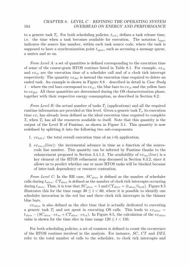
104CHAPTER 8. LEVEL C – REFINING THE OPERATING SYSTEM
OVERHEAD ON ENERGY AND PERFORMANCE
to a generic task Ti. For both scheduling policies, trel,i defines a task release time,i.e. the time when a task becomes available for execution. The notation lsyncindicates the source line number, within each task source code, where the task issupposed to have a synchronization point tsync, such as accessing a message queue,a mutex and so on.
From Level A: a set of quantities is defined corresponding to the execution timeof some of the coarse-grain RTOS routines listed in Table 8.1. For example, exscand exct are the execution time of a scheduler call and of a clock tick interruptrespectively. The quantity exdel is instead the execution time required to delete anended task. An example is shown in Figure 8.8 – described in detail in Case Study1 – where the red bars correspond to exsc, the blue bars to exct and the yellow barsto exdel. All these quantities are determined during the OS characterization phase,together with their respective energy consumption, as described in Section 8.2.
From Level B: the actual number of tasks Ti (applications) and all the requiredruntime information are provided at this level. Given a generic task Ti, its executiontime exi has already been defined as the ideal execution time required to completeTi when Ti has all the resources available to itself. Note that this quantity is theoutput of the Level B of Funtime, as shown in Figure 3.1. This quantity is nowredefined by splitting it into the following two sub-components:
1. extot,i: the total overall execution time of an i-th application.
2. exinc,i(line): the incremental advance in time as a function of the source-code line number. This quantity can be inferred by Funtime thanks to theenhancement proposed in Section 3.4.1.2. The availability of exinc(line) is akey element of the RTOS refinement step discussed in Section 8.3.2, since itallows us to predict whether one or more RTOS tasks will be blocked becauseof inter-task dependency or resource contention.
From Level C: In the RR case, SCslice is defined as the number of schedulercalls during tslice. CTslice is defined as the number of clock tick interrupts occurringduring tslice. Thus, it is true that SCslice = 1 and CTslice = (tslice/ttick). Figure 8.5illustrates this for the time range 30 ≤ t < 60, where it is possible to identify onescheduler invocation in the red bar and three clock tick interrupts in the thinnerblue bars.
exslice is also defined as the slice time that is actually dedicated to executinga generic task Ti and not spent in executing OS calls. This leads to exslice =tslice − (SCslice · exsc + CTslice · exct). In Figure 8.5, the calculation of the exslicevalue is shown for the time slice in time range 120 ≤ t < 150.
For both scheduling policies, a set of counters is defined to count the occurrenceof the RTOS routines involved in the analysis. For instance, SC, CT and DELrefer to the total number of calls to the scheduler, to clock tick interrupts and
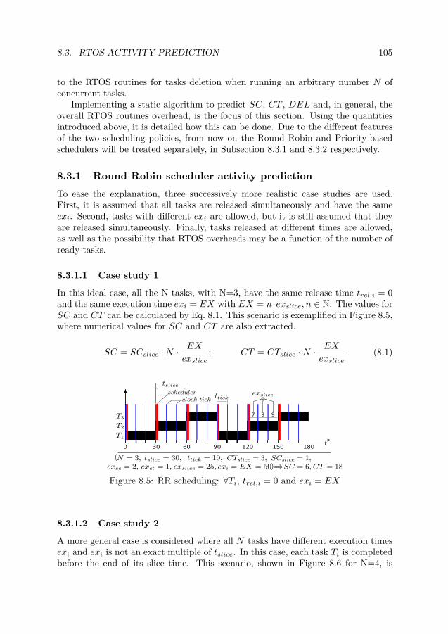
8.3. RTOS ACTIVITY PREDICTION 105
to the RTOS routines for tasks deletion when running an arbitrary number N ofconcurrent tasks.
Implementing a static algorithm to predict SC, CT , DEL and, in general, theoverall RTOS routines overhead, is the focus of this section. Using the quantitiesintroduced above, it is detailed how this can be done. Due to the different featuresof the two scheduling policies, from now on the Round Robin and Priority-basedschedulers will be treated separately, in Subsection 8.3.1 and 8.3.2 respectively.
8.3.1 Round Robin scheduler activity predictionTo ease the explanation, three successively more realistic case studies are used.First, it is assumed that all tasks are released simultaneously and have the sameexi. Second, tasks with different exi are allowed, but it is still assumed that theyare released simultaneously. Finally, tasks released at different times are allowed,as well as the possibility that RTOS overheads may be a function of the number ofready tasks.
8.3.1.1 Case study 1
In this ideal case, all the N tasks, with N=3, have the same release time trel,i = 0and the same execution time exi = EX with EX = n·exslice, n ∈ N. The values forSC and CT can be calculated by Eq. 8.1. This scenario is exemplified in Figure 8.5,where numerical values for SC and CT are also extracted.
SC = SCslice ·N ·EX
exslice; CT = CTslice ·N ·
EX
exslice(8.1)
0 30 60 90 120 150 180t
7 9 9
+
Figure 8.5: RR scheduling: ∀Ti, trel,i = 0 and exi = EX
8.3.1.2 Case study 2
A more general case is considered where all N tasks have different execution timesexi and exi is not an exact multiple of tslice. In this case, each task Ti is completedbefore the end of its slice time. This scenario, shown in Figure 8.6 for N=4, is

106CHAPTER 8. LEVEL C – REFINING THE OPERATING SYSTEM
OVERHEAD ON ENERGY AND PERFORMANCE
highlighted in grey boxes. When this condition occurs, the scheduler is called atthe end of the task and, unless the ready task queue is empty, a context switchoccurs, even if the slice time has not yet expired. This is done to minimize theperformance loss. Note that the behavior described is valid for RTEMS. In thiscase, a more general formula is needed to determine SC and CT .
0 40 80 160120 200 240t
260 300 330 370
+
7 3 7 9 4 9 9 9 5 9 9 7
+ + +
Figure 8.6: Round Robin scheduling: ∀Ti, trel,i = 0, exi 6= EX and exi 6= exj
The quantities Qi and Ri are defined as the quotient and the remainder of thedivision exi/exslice for a generic task Ti. Ri is the portion of Ti for which theexecution time is smaller than a slice time, that is 0 ≤ Ri < exslice. The value ofRi is shown in Figure 8.6 for each of the 4 tasks considered in this example. Letthen SCrem,i and CTrem,i be the number of calls to the scheduler and of clock ticksoccurring during the time Ri. The values of SCrem,i and CTrem,i can be expressedas in Eq. 8.2 and 8.3 respectively.
SCrem,i ={
0 if Ri = 01 if Ri > 0 (8.2)
CTrem,i =
1 if Ri ≤ (ttick − exsc − exct)
1 +⌈Ri − (ttick − exsc − exct)
ttick − exct
⌉if Ri > (ttick − exsc − exct)
(8.3)The total number of calls to the scheduler SC and clock tick interrupts CT
is now calculated through an iterative process, where the number of iterationscorresponds to the number of tasks N. During each iteration, the value of SC andCT is incremented. The main steps are shown in Algorithm 1 below.
Algorithm 1 Assumptions: trel,i = 0, exi 6= exj
SC,CT ← 0;for i = 1 to N doSC ← SC + SCslice ·Qi + SCrem,i;CT ← CT + CTslice ·Qi + CTrem,i;
end for

8.3. RTOS ACTIVITY PREDICTION 107
8.3.1.3 Case study 3
A more real case is considered where N tasks have arbitrary release times trel,i andexecution times exi, as shown in Figure 8.7. In addition, it is assumed that theexecution time of some OS functionalities is related to the number of ready tasksrdy(t) at the time t when such functionalities are triggered. Thus, in this case exscand exct are not constant figures any more, but they depend on rdy(t) and can bedenoted as exsc(rdy(t)) and exct(rdy(t)) respectively.
0 40 80 160120 200 240t
280 320 350
Figure 8.7: Round Robin scheduling: ∀Ti, trel,i 6= 0, exi 6= EX, exi 6= exj ,exsc(rdy(t)) and exct(rdy(t))
When calculating the value of SC and CT , it is therefore also necessary todetermine the value of rdy(t). This process can be eased by restricting the eval-uation of rdy(t) to specific time points, which correspond either to a task releasetime trel,i or completion time tend,i. The reason is that the value of rdy(t) remainsunchanged for all the other values of t. The result is a static decomposition ofthe whole scheduling into multiple time windows wi. This is shown in Figure 8.7,where five time windows [w1, w5] are identified for three tasks and highlighted bydifferent-color areas. In detail, whenever a new time window starts and rdy(t) iscalculated, the ending time of the same time window is identified as the minimumtime between the tend,i for each ready task and the next closest release time trel.Once the time window has been defined, the values of SC and CT for that timewindow are calculated and added to the old ones calculated in the previous win-dow. This process is iterated until all tasks are completed. Note that, even inthis more elaborated implementation, the proposed OS prediction algorithm stillhas an execution time proportional to the number of tasks involved, not to theirexecution time exi. Thus, it is still extremely fast. The pseudo-code for the mainsteps described above is reported in Algorithm 2.
8.3.2 Prediction of Priority-Driven Scheduler ActivityAlso in this case, to ease the explanation, two successively more realistic case studiesare used. First, it is assumed that all independent tasks not competing for sharedresources, but with different release times for the tasks, are allowed, as well as thepossibility that RTOS overheads may be a function of the number of ready tasks.Second, the same assumptions are kept as for the first case study, except that inter-dependent tasks which can compete for shared resources are also allowed. For a

108CHAPTER 8. LEVEL C – REFINING THE OPERATING SYSTEM
OVERHEAD ON ENERGY AND PERFORMANCE
Algorithm 2 trel,i 6= 0, exi 6= exj , exsc(rdy(t)), exct(rdy(t))SC(rdy(t)) = CT (rdy(t)) = 0;total execution time left e_tot_left←
∑Ni=1 exi;
time t← 0;while e_tot_left > 0 dofor i = 1 to N dordy(t)← number of ready tasks at time t;Trdy[i]← which tasks are ready at time t;
end forfor each Trdy[i] at time t docalculate its ending time tend,i;
end fortend_min ← min between each tend,i and next closest trel;update SC(tend_min − t, rdy(t));update CT (tend_min − t, rdy(t));update e_tot_left;t← tend_min
end while
successful OS prediction in this second case study, the importance is demonstratedof the extension to the GCC compiler described in Section 3.4.1.2. Note that,although in this chapter RTEMS is taken as the reference OS, the methodology isgeneral and can be adapted to any OS.
8.3.2.1 Case study 1
This case study considers the case whereN independent tasks with priority Π(T1) >Π(Ti) > Π(TN ) have arbitrary release times trel,i and where the execution time ofsome OS functionalities is dependent on the number of ready tasks rdy(t) at thetime t when such functionalities are triggered. For this reason, exsc, exct and exdelare not constant figures, but depend on rdy(t) and can be denoted as exsc(rdy(t)),exct(rdy(t)) and exdel(rdy(t)) respectively. The availability of the rdy(t) value alsoallows us to infer the possible occurrence of the OS idle task, a condition that istrue for rdy(t) = 0. For this case study, only the component extot,i of the quantityexi is needed.
Figure 8.8 is used as a reference during the algorithm description. Three in-dependent tasks are shown, T1 and T3 being the highest and lowest priority taskrespectively. At the figure bottom, the trel,i and tend,i value associated with eachtask is indicated. Note that, while the value of trel,i is user-assigned, the value oftend,i is calculated at run-time by the prediction algorithm. In addition, althoughtrel,i could in principle be assigned any time value, this value is seen and evaluatedonly at the occurrence of the next closest clock tick, when the scheduler is invoked.For this reason, it is assumed that either the Funtime user or a Funtime routine

8.3. RTOS ACTIVITY PREDICTION 109
can take care of always setting a task trel,i at a time which is a multiple of ttick.The value of tend,i can instead occur at any time, since the scheduler is called bythe OS routine that deletes the ended task. This is represented by the yellow barsin Figure 8.8.
0 30 60 90 120 150t
9
9 9
99 9
7 9
7
7
9 9 9
180
1
32 2
Figure 8.8: 3 independent tasks T1, T2 and T3. trel,i 6= trel,j
The value of trel,i and tend,i is of great importance for the whole predictionalgorithm, since evaluation is restricted to only these specific times. The reasonis that there is no other time when a variation in the tasks state or in the tasksready queue can be encountered. The result is a static decomposition of the wholescheduling into multiple time windows wi. This is shown in Figure 8.8, where fivetime windows [w1, w5] are identified for three tasks and highlighted by different-color areas.
In detail, whenever a new time window starts, the following operations areperformed.
1. The number of ready tasks rdy(t) is calculated. If rdy(t) = 0, the OS Idletask is expected to run for the next time window wi. This case is shown inFigure 8.8 at time t = 42.
2. The ready tasks are sorted according to their priority. The highest-prioritytask TH is expected to run for the next time window wi. For instance, notethat, as shown in Figure 8.8 at time t = 110, task T3 is preempted by taskT1, which has higher priority.
3. The ending time of a time window is identified as the minimum time betweenthe tend,i of the task running in that window and the next closest release timetrel,i.
4. The values of SC, CT and DEL are updated with the related contributionsgiven in the present window. Such contributions are defined as SCw, CTwand DELw.
5. This process is iterated until all tasks are completed.

110CHAPTER 8. LEVEL C – REFINING THE OPERATING SYSTEM
OVERHEAD ON ENERGY AND PERFORMANCE
The value of tend,i, within each time window, is determined through the followingconsiderations. First, the initial OS overhead for the window being estimated istaken into account and the current time tcurrent is updated. For instance, when anew window starts after another task has ended, the OS routine for task deletion isalways executed (yellow bar), followed by a call to the scheduler (red bar). Thus,if the beginning of window w5 in Figure 8.8 is taken as an example, it is true thatexdel + exsc = 2 + 2 = 4 ⇒ tcurrent = 133 + 4 = 137. Second, the time differenceis calculated between the next closest clock tick and the current time, the currenttime is incremented of a quantity equal to the calculated time difference and thatdifference is subtracted from the total task execution time extot,i. This is done toend up exactly at the time when a clock tick occurs and thus ease the calculationof the number of total clock ticks happening until the end of the task. Referringagain to Figure 8.8, this step takes us from an initial tcurrent = 137 to a finaltcurrent = 140. Third, the number of clock tick interrupts for the present window iscalculated. This quantity has been previously defined as CTw. It is true that CTw =d time_leftittick−exct
e. For the example considering w5, it is true that CTw = d 3810−1e = 5.
Finally, tend,i can be calculated as tend,i = tcurrent + time_lefti + exct · CTw. Inour case, tend,3 = 140 + 38 + 1 · 5 = 183, which is correct.
Note that, although the proposed OS behavior prediction algorithm exhibitsan iterative behavior, it still has an execution time proportional to the number ofwindows defined by the algorithm, and not to the tasks execution time extot,ii.Thus, it is still fast and clearly faster than running the actual OS.
8.3.2.2 Case study 2
In this realistic case study, all the considerations made in Case study 1 are keptvalid, but interdependent tasks that can compete for shared resources are alsoallowed. Unlike the previous case study, here the exinc,i(line) component of thequantity exi is also needed.
By interdependent task is meant a task that, at some point of its execution,reaches a synchronization point tsync where it needs to wait for data from anothertask before being able to continue. As an example, consider Figure 8.9: at timet = 33, the highest priority task T1 attempts to receive data from a message queue,but fails and becomes blocked, since the queue is empty. At time t = 83, T2successfully sends some data into the same message queue and then is preemptedby T1, which has now been unblocked and can thus resume its execution.
A shared resource could be a memory, a mutex or, in general, a serially-accessibleresource. A conflict occurs when multiple tasks try to access the same resource atthe same time. In general, the part of code dealing with accessing a resource isdefined as a critical section and normally it cannot be preempted, not even by ahigher-priority task. This case is visible in Figure 8.9: at time t = 132, the lowest-priority task T4 successfully locks a mutex and enters its critical section. The accessto a shared resource R is shown as a white-filled rectangle. At time t = 150, T4is preempted by T3 and, in turn, at time t = 180, T3 is preempted by T2. Then

8.3. RTOS ACTIVITY PREDICTION 111
9397
2
993
27 9 9
2
0 30 60 90 120 150 t
7 9
180
3
9
7
7
210 240 270 300 330
9
9 9
7
R R
R9 9
9 9
91 7
7
3
2
2 9
9 9 9
4 322
Figure 8.9: 3 inter-dependent tasks T1, T2, T3 and T4. trel,i 6= trel,j
at time t = 213, T2 also tries to access resource R by locking the same mutexpreviously locked by T4. However, the locking attempt fails and T2 is blocked untilT4 releases the mutex at time t = 265.
This scenario is known as priority inversion and generally refers to the caseof a high-priority task being blocked by a lower-priority task. Some techniqueshave been developed to avoid this problem. Two of them are known as priorityinheritance and priority ceiling. Observe that the goal of this chapter is not to findthe best scheduling policy for a given scenario, but rather to show how, providedthere is a priority-driven scheduling for a given scenario, Funtime can predict theOS components overhead. Nevertheless, compliance to the priority inheritance andpriority ceiling techniques can be enabled in Funtime too, as part of the priorityprediction algorithm. The user of Funtime will choose which policy to use.
This case study accounts for the implications of having interdependent tasksthat can compete for shared resources, since these factors can heavily affect theamount of OS overhead, i.e. number of context switches, occurrence and durationof the OS Idle task, etc. For example, it is only by knowing at which point in timeT1 tries to read from its message queue that it is possible to estimate the duration ofthe OS Idle task. As another example, by knowing when T4 tries to lock its mutex,it can be predicted whether T4 will be able to get the lock before T3 is released ornot. If it does, then this is the scenario shown in Figure 8.9 and described above.If not, T4 will be able to lock its mutex only after T2 and T3 have finished. In thislatter case, T2 would not be blocked and therefore two context switches less wouldbe counted.
However, to be able to predict the time point tsync when a task tries to accessan OS resource, like a message queue or a mutex (see the top of Figure 8.9), theonly knowledge of the total task execution time extot,i is no longer enough. Instead,the following two conditions must also be satisfied:
1. It must be possible to evaluate the advance of time with the granularity ofa single source-code line. This quantity has been defined as exinc,i(line) andcan be retrieved by instrumenting the compiler as described in Section 3.4.1.2.
2. The Funtime user must specify at what source-code line lsync the synchro-nization point occurs and what dependency relation exists. This information

112CHAPTER 8. LEVEL C – REFINING THE OPERATING SYSTEM
OVERHEAD ON ENERGY AND PERFORMANCE
is provided as part of the UCS.
From the two points above, it gives that tsync = exinc(lsync).As in Case study 1, the proposed OS prediction algorithm relies on taking
decisions at specific time points, which correspond to the end of temporal windowswi. The only difference is that not only trel,i and tend,i are used to identify a windowedges, but also the time points where a task reaches a synchronization point. Thisis shown in Figure 8.9, where 13 windows are identified.
In the case of interdependent tasks, in order to run an application on the devel-opment host at Level B (Algorithmic Level), it is necessary that the Funtime usermanually provides a value to the variables that, at Level C (Refinement Level),would be assigned at a synchronization point. It is emphasized that Level B is theonly level where an application is run in Funtime (see Figure 3.1). In case that anapplication takes different branches depending on the value received, the Funtimeuser chooses the values according to the specific needs, so to have a trace of pri-mary transactions available for the different possibilities. Later on, he/she can alsospecify a percentage value corresponding to the frequency each branch is taken.Note instead that, at Level C, no application is run at all, as well as no OperatingSystem.
Algorithm 3 reports the pseudo-code for the main steps described in Case study1 above. The text in red color instead distinguishes the extra component neededto account for Case study 2.
Algorithm 3/* Initialize all the OS quantities to zero */SC(rdy(t)) = CT (rdy(t)) = · · · = DEL(rdy(t))← 0;total execution time left e_tot_left←
∑Ni=1 exi;
current time tcurrent ← 0;while e_tot_left > 0 dofor i = 1 to N dordy(t)← number of ready tasks at time t;TH(t)← highest priority task ready at time t;
end forcalculate TH ending time tend,TH
;tnext ← min(tend,TH
, closest trel, closest tsync);/* Update all the OS quantities */update SC(tnext − tcurrent, rdy(t));update CT (tnext − tcurrent, rdy(t));...update DEL(tnext − tcurrent, rdy(t));update e_tot_left;tcurrent ← tnext
end while

8.4. VALIDATION OF REFINEMENT ACCURACY 113
8.4 Validation of Refinement Accuracy
Validation of the refinement presented in this chapter has been carried out both forthe Round Robin and Priority-driven scheduler. The accuracy of the refinementestimation, for both the OS energy and latency, has been validated against gate-level estimation. The reason is two-fold: first, gate level is very accurate; second,IP-level energy models and the OS refinements were achieved based on gate-levelcharacterization.
8.4.1 Round Robin schedulerThe SoC platform used for validation is the same as that used for the OS charac-terization and shown in Figure 8.2. The goal is to verify the accuracy of Funtime inpredicting energy and execution time for a software environment where two tasksT1 and T2 run on top of the RTEMS OS and are scheduled using Round Robin.The values of the clock tick period ttick and of the time slice period tslice have beenset to 1ms and 3ms respectively.
T1 and T2 are synthetic applications that have been chosen on purpose withdifferent execution times ex1 6= ex2, but with the same release times trel,1 = trel,2 =0. Such applications are different from those used during the OS characterization.
The results have been collected in Table 8.2, which has been drawn on two linesdue to the lack of space. The table is itself split into three horizontal subtablesconsidering an increasing number of sources of inaccuracy. Subtable 1 only considersthe error deriving from the OS characterization described in Section 8.2, while ex1and ex2, as well as the OS activity are measured from gate level. Subtable 2 hastwo sources of inaccuracy: the OS characterization and the OS activity prediction,described in Section 8.2 and 8.3.1 respectively, while ex1 and ex2 are measured.Finally, Subtable 3 considers three sources of inaccuracy: the first two are the sameas for Subtable 2, while the third comes from using Funtime (Level A and B) to alsoderive ex1 and ex2. Note that the top part of the table reports figures related tothe two tasks T1 and T2, independently of the OS; the bottom part is instead meantto show the OS overhead. The energy values shown refer to the Leon3 processor.
The RTEMS functionalities that are accounted for in Table 8.2 are, from left toright, the clock tick interrupt, the invocation to the scheduler resulting in a contextswitch and the invocation to the scheduler not resulting in a context switch. Foreach such functionality, a comparison is made between energy and time valuesextracted from a gate-level simulation and those inferred by Funtime. In any ofthe three subtables, the results show that the Funtime accuracy increases withthe number of OS system calls. For example, the accuracy achieved for the clocktick interrupt, which occurs 108 times, is much higher than that achieved for thescheduler invocation without context switch, which occurs only eight times. Fromthe OS activity prediction perspective, it is straightforward that a 1-unit errorweighs more on a total of 8 units rather than 108. However, it is emphasized thatthe Funtime methodology is meant to be used on extensive use-case scenarios, where
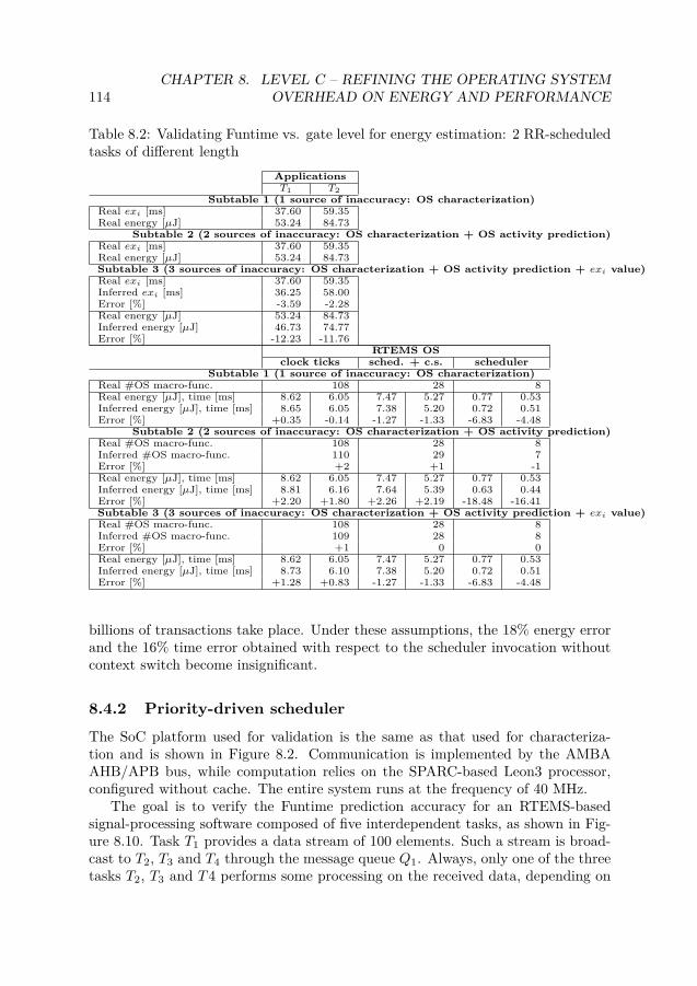
114CHAPTER 8. LEVEL C – REFINING THE OPERATING SYSTEM
OVERHEAD ON ENERGY AND PERFORMANCE
Table 8.2: Validating Funtime vs. gate level for energy estimation: 2 RR-scheduledtasks of different length
ApplicationsT1 T2
Subtable 1 (1 source of inaccuracy: OS characterization)Real exi [ms] 37.60 59.35Real energy [µJ] 53.24 84.73
Subtable 2 (2 sources of inaccuracy: OS characterization + OS activity prediction)Real exi [ms] 37.60 59.35Real energy [µJ] 53.24 84.73Subtable 3 (3 sources of inaccuracy: OS characterization + OS activity prediction + exi value)Real exi [ms] 37.60 59.35Inferred exi [ms] 36.25 58.00Error [%] -3.59 -2.28Real energy [µJ] 53.24 84.73Inferred energy [µJ] 46.73 74.77Error [%] -12.23 -11.76
RTEMS OSclock ticks sched. + c.s. scheduler
Subtable 1 (1 source of inaccuracy: OS characterization)Real #OS macro-func. 108 28 8Real energy [µJ], time [ms] 8.62 6.05 7.47 5.27 0.77 0.53Inferred energy [µJ], time [ms] 8.65 6.05 7.38 5.20 0.72 0.51Error [%] +0.35 -0.14 -1.27 -1.33 -6.83 -4.48
Subtable 2 (2 sources of inaccuracy: OS characterization + OS activity prediction)Real #OS macro-func. 108 28 8Inferred #OS macro-func. 110 29 7Error [%] +2 +1 -1Real energy [µJ], time [ms] 8.62 6.05 7.47 5.27 0.77 0.53Inferred energy [µJ], time [ms] 8.81 6.16 7.64 5.39 0.63 0.44Error [%] +2.20 +1.80 +2.26 +2.19 -18.48 -16.41Subtable 3 (3 sources of inaccuracy: OS characterization + OS activity prediction + exi value)Real #OS macro-func. 108 28 8Inferred #OS macro-func. 109 28 8Error [%] +1 0 0Real energy [µJ], time [ms] 8.62 6.05 7.47 5.27 0.77 0.53Inferred energy [µJ], time [ms] 8.73 6.10 7.38 5.20 0.72 0.51Error [%] +1.28 +0.83 -1.27 -1.33 -6.83 -4.48
billions of transactions take place. Under these assumptions, the 18% energy errorand the 16% time error obtained with respect to the scheduler invocation withoutcontext switch become insignificant.
8.4.2 Priority-driven schedulerThe SoC platform used for validation is the same as that used for characteriza-tion and is shown in Figure 8.2. Communication is implemented by the AMBAAHB/APB bus, while computation relies on the SPARC-based Leon3 processor,configured without cache. The entire system runs at the frequency of 40 MHz.
The goal is to verify the Funtime prediction accuracy for an RTEMS-basedsignal-processing software composed of five interdependent tasks, as shown in Fig-ure 8.10. Task T1 provides a data stream of 100 elements. Such a stream is broad-cast to T2, T3 and T4 through the message queue Q1. Always, only one of the threetasks T2, T3 and T4 performs some processing on the received data, depending on

8.4. VALIDATION OF REFINEMENT ACCURACY 115
Table 8.3: Validating Funtime vs. gate level for energy estimation: priority-drivenscheduling
ApplicationsT1 T2 T3 T4 T5
Subtable 1 (1 source of inaccuracy: OS characterization)Real exi [ms] 0.3 11.3 5.1 14.0 9.8Real en. [µJ] 0.5 15.8 7.1 19.5 13.7
Subtable 2 (2 sources of inaccuracy: OS characterization + OS activity prediction)Real exi [ms] 0.3 11.3 5.1 14.0 9.8Real en. [µJ] 0.5 15.8 7.1 19.5 13.7Subtable 3 (3 sources of inaccuracy: OS characterization + OS activity prediction + exi value)Real exi [ms] 0.3 11.3 5.1 14.0 9.8Inferred exi [ms] 0.3 9.8 5.0 12.8 8.1Error [%] -5.4 -13.0 -1.2 -8.5 -16.3Real en. [µJ] 0.5 15.8 7.1 19.5 13.7Inferred en. [µJ] 0.5 14.8 7.6 19.3 12.2Error [%] -6.3 -5.9 +6.2 -1.4 -10.5
RTEMS OSclock ticks msg q. broadcast(3) msg q. send msg q. receive
+ c.s. + c.s. + c.s.Subtable 1 (1 source of inaccuracy: OS characterization)
Real #OS macro-func. 1174 100 100 400Real en. [µJ], time [ms] 89.0 61.6 44.1 31.4 25.8 18.3 99.0 71.5Inferred en. [µJ], time [ms] 94.1 65.7 43.4 30.7 24.7 17.5 97.5 69.1Error [%] +5.7 +6.6 -1.5 -2.4 -4.0 -4.6 -1.5 -3.4
Subtable 2 (2 sources of inaccuracy: OS characterization + OS activity prediction)Real #OS macro-func. 1174 100 100 400Inferred #OS macro-func. 1263 100 100 400Error [#] +89 0 0 0Real en. [µJ], time [ms] 89.0 61.6 44.1 31.4 25.8 18.3 99.0 71.5Inferred en. [µJ], time [ms] 101.2 70.7 43.4 30.7 24.7 17.5 97.5 69.1Error [%] +13.7 +14.8 -1.5 -2.4 -4.0 -4.6 -1.5 -3.4
Subtable 3 (3 sources of inaccuracy: OS characterization + OS activity prediction + exi value)Real #OS macro-func. 1174 100 100 400Inferred #OS macro-func. 1234 100 100 400Error [#] +60 0 0 0Real en. [µJ], time [ms] 89.0 61.7 44.1 31.4 25.8 18.3 99.0 71.5Inferred en. [µJ], time [ms] 98.9 69.1 43.4 30.7 24.7 17.5 97.5 69.1Error [%] +11.1 +12.0 -1.5 -2.4 -4.0 -4.6 -1.5 -3.4
the actual data value. The processed data is then sent into the message queueQ2 and reaches the output process T5. This modeling flow could be, for instance,representative of an equalizer.
Figure 8.10: RTEMS-based signal-processing software
The RTEMS clock tick period ttick has been set to 200µs. The task priorityhas been assigned as follows: Π(T5) > Π(T2) > Π(T3) > Π(T4) > Π(T1). Thismeans that T5 and T1 have the highest and lowest priority respectively. This isdone since the system is expected to be immediately ready to operate whenever
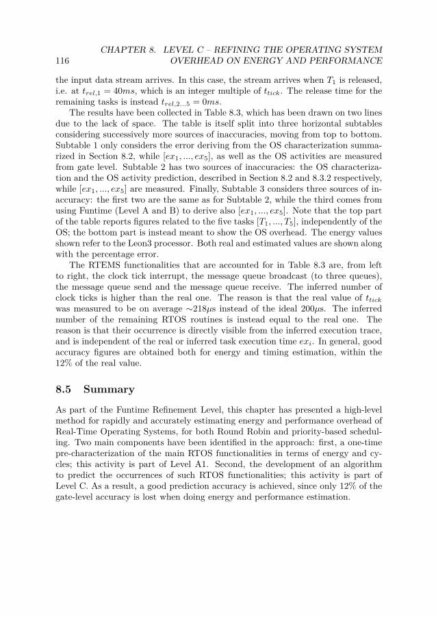
116CHAPTER 8. LEVEL C – REFINING THE OPERATING SYSTEM
OVERHEAD ON ENERGY AND PERFORMANCE
the input data stream arrives. In this case, the stream arrives when T1 is released,i.e. at trel,1 = 40ms, which is an integer multiple of ttick. The release time for theremaining tasks is instead trel,2...5 = 0ms.
The results have been collected in Table 8.3, which has been drawn on two linesdue to the lack of space. The table is itself split into three horizontal subtablesconsidering successively more sources of inaccuracies, moving from top to bottom.Subtable 1 only considers the error deriving from the OS characterization summa-rized in Section 8.2, while [ex1, ..., ex5], as well as the OS activities are measuredfrom gate level. Subtable 2 has two sources of inaccuracies: the OS characteriza-tion and the OS activity prediction, described in Section 8.2 and 8.3.2 respectively,while [ex1, ..., ex5] are measured. Finally, Subtable 3 considers three sources of in-accuracy: the first two are the same as for Subtable 2, while the third comes fromusing Funtime (Level A and B) to derive also [ex1, ..., ex5]. Note that the top partof the table reports figures related to the five tasks [T1, ..., T5], independently of theOS; the bottom part is instead meant to show the OS overhead. The energy valuesshown refer to the Leon3 processor. Both real and estimated values are shown alongwith the percentage error.
The RTEMS functionalities that are accounted for in Table 8.3 are, from leftto right, the clock tick interrupt, the message queue broadcast (to three queues),the message queue send and the message queue receive. The inferred number ofclock ticks is higher than the real one. The reason is that the real value of ttickwas measured to be on average ∼218µs instead of the ideal 200µs. The inferrednumber of the remaining RTOS routines is instead equal to the real one. Thereason is that their occurrence is directly visible from the inferred execution trace,and is independent of the real or inferred task execution time exi. In general, goodaccuracy figures are obtained both for energy and timing estimation, within the12% of the real value.
8.5 Summary
As part of the Funtime Refinement Level, this chapter has presented a high-levelmethod for rapidly and accurately estimating energy and performance overhead ofReal-Time Operating Systems, for both Round Robin and priority-based schedul-ing. Two main components have been identified in the approach: first, a one-timepre-characterization of the main RTOS functionalities in terms of energy and cy-cles; this activity is part of Level A1. Second, the development of an algorithmto predict the occurrences of such RTOS functionalities; this activity is part ofLevel C. As a result, a good prediction accuracy is achieved, since only 12% of thegate-level accuracy is lost when doing energy and performance estimation.
Chapter 9
Conclusions and Future Work
This chapter summarizes the key features of Funtime that have been discussed inthis thesis work and proposes extensions to the present Funtime framework as partof the future work.
9.1 Conclusions
The present work has described in detail a system-level framework for energy andperformance estimation, which has been called Funtime. The need of having effi-cient system-level estimation (SLE) tools is justified by the increasing broadnessof the design space at the system level, which makes it very difficult to take thebest architectural decisions. Decisions taken at the system level, early in the designcycle, are however essential in affecting the quality of the final design. Taking suchdecisions manually, based on the experience matured from previous designs andon rules of thumb, as it has been done so far, is not a feasible approach anymore.Efficient SLE tools are therefore necessary to automate the activities performed atsystem level. Specifically, such tools can be used to perform design-space explo-ration and as a basis for system-level synthesis.
Several of today’s approaches to system-level estimation and design in general,such as Transaction-Level Modeling, still rely on the architectural simulation of thetarget. This implies an extra engineering effort, since a new executable specifica-tion of the target has to be written. Besides, although at a high abstraction level,architectural simulation may still be too slow when modeling large use-case scenar-ios. Unlike these approaches, Funtime does not rely on a high-level simulation ofthe target to carry out estimation. Instead, its estimation activity is based on thefollowing three layers.
First, a characterization layer – the IP Level (Level A) – which creates IP energyand performance models. These are not executable models, since they come in theform of either look-up tables or analytical expressions. Although time-consuming,since performed on a back-annotated gate-level netlist and for each IP transaction,
117

118 CHAPTER 9. CONCLUSIONS AND FUTURE WORK
this step still makes sense since it is a one-time activity performed by the IP providerand it gives high accuracy to the whole estimation tool. A case study has beenpresented in Chapter 4, where one such IP model has been implemented for aLeon3 processor. The accuracy of the model has then been validated against gate-level estimation and has shown to be within 15%. Level A also models the impactthat the external communication link, connecting different IPs, has on individualIP transactions. Chapter 5 presents a case study about switching from a bus-basedSoC to a NoC, and uses the same Leon3 processor as a reference IP. The accuracyof the new model has been measured to be within 10% of the gate-level estimation.
Second, the actual estimation layer – the Algorithmic Level (Level B) – wherethe energy and performance for individual applications are predicted. This layerrelies on inferring a trace of target transactions, called primary transactions, byonly executing the application on the evaluation host while profiling it with target-specific information. This is also the step that confers high estimation speed tothe methodology, and is the end user entry point to Funtime. A case study hasbeen presented in Chapter 6, where Funtime has been used to estimate energy andexecution time for a set of benchmark applications. Funtime estimation accuracyhas been validated against gate-level estimation and proved to be within 15%.Funtime estimation speed has also been validated against transaction-level modeling(TLM), showing an average speedup of 30X.
Third, another estimation layer – the Refinement Level (Level C) – which factorsin some non-idealities neglected at the Level B, where each application was con-sidered individually and as if it had all the system resources at its disposal. Suchnon-idealities, which introduce a variation in the system overall energy and perfor-mance, include the impact of transactions interdependency, the effects of caches,of bus contention and of an operating system. As opposed to the AlgorithmicLevel, the Refinement Level does not run the applications at all, not even on theevaluation host. Instead, it statically applies a set of algorithms, specific to eachindividual refinement, that allow us to infer a trace of extra transactions, calledsecondary transactions, to be added to the original trace of primary transactions.Since every transaction in the resulting trace has been characterized for energy andcycles, the total system energy and performance can thus be predicted. The refine-ments concerning transactions interdependency and caches have been presented inthe Chapter 6, together with the Algorithmic Level, due to the tight relation thatthese refinements have with inferring transactions for individual applications. Acase study about predicting bus contention has been proposed in Chapter 7, wherea homogeneous bus-based MPSoC using Leon3 processors has been taken as a ref-erence platform. Round-robin arbitration scheme has been used. The predictionaccuracy, for the set of applications used, has shown to be within 2% of the gate-level estimation. Chapter 8 has instead presented a case study about predictingthe overhead of operating systems, in terms of energy and performance overhead.RTEMS has been used as a reference OS, for both round-robin and priority-driventask scheduling. The prediction accuracy has been validated also in this case andit has shown to be within 12% of the gate-level estimation.
9.2. FUTURE WORK 119
It is emphasized that, because of the very large size of real use-cases and thelarge amount of factors to be considered when doing system-level estimation, itwas not possible to deal with all these aspects within this work. Instead, smalleruse-cases have been used as case studies and sensible simplifications have beenmade. As a consequence, the Funtime framework presented in this thesis comes asa proof of concept, with the goal of showing the overall feasibility of the Funtimeapproach as a system-estimation tool. Further extensions are required to make thisframework more general and complete, as is discussed in the next section.
9.2 Future Work
Despite the detailed presentation that was given in this thesis work, further devel-opment is needed for Funtime to be used as a complete, stand-alone tool. Amongthe aspects that can be improved, the following ones are considered to be the mostrelevant:
• The Funtime User Interface should be formalized. Specifically, the Archi-tecture Specification (AS) and the Use-Case Specification (UCS) should beexpressed in form of files. Such files could be written for example in XML,which is an efficient machine-readable format. In fact, although throughoutthis thesis it has been assumed that the end-user of Funtime is a humanbeing, in reality Funtime could just be the estimation component within adesign-space exploration (DSE) tool or system-level synthesis tool.
• At the Level A1, the implementation of an energy and performance modelfor a Leon3 processor has been presented as a case study. Although for thisexample no physical layout has been carried out, this activity is consideredimportant for two main reasons: first, it would improve the accuracy of theIP model itself; second, it would provide exact information on the IP area,which is useful to estimate the global wires length as part of the preliminaryfloorplan activity.
• At the Level B, the instrumentation for applications mapped to software canbe enhanced with the possibility to include the contribution coming fromexternal library functions which, as discussed in Section 3.4.1, is not possibleat present. In the context of the present work, the problem has been avoidedby implementing our own routines instead of using the library ones and bycommenting out all the print-related routines.
• At the Level C, as far as bus refinement is concerned, this work has onlyconsidered a homogeneous MPSoC based on Leon3 processors. It would beinteresting to see how the approach that has been proposed in this work canbe adapted to the case of heterogeneous MPSoCs as well. This case wouldprobably be more challenging to model, because of the diverse patterns shownby different resources when accessing the bus. In addition, the bus contention
120 CHAPTER 9. CONCLUSIONS AND FUTURE WORK
refinement proposed in Chapter 7 only considers the case of a round-robinbus arbitration scheme. The priority-driven case should be considered andmodeled as well.
• All the refinements have been so far investigated and presented independently.A significant case study should be taken where all such refinements are ap-plied together according to the guidelines discussed in Section 3.9. Note thatthe main issue that had to be faced in this work when trying to deal withsignificant and realistic examples was the extremely long time required to rungate-level simulation and estimation as part of the Funtime accuracy valida-tion. This fact has often led to selecting smaller examples as case studies,which were anyhow sufficient to prove the validity of the approach.

Bibliography
[1] AEROFLEX GAISLER. http://www.gaisler.com.
[2] GNU Compiler Collection. http://gcc.gnu.org.
[3] GNU Compiler Collection Internals. http://gcc.gnu.org.
[4] RTEMS Homepage. http://www.rtems.com.
[5] M. AbdElSalam Hassan, K. Sakanushi, Y. Takeuchi, and M. Imai. Enablingrtos simulation modeling in a system level design language. In Design Automa-tion Conference, 2005. Proceedings of the ASP-DAC 2005. Asia and SouthPacific, volume 2, pages 936 – 939 Vol. 2, january 2005.
[6] Vikram S. Adve and Mary K. Vernon. Parallel program performance predictionusing deterministic task graph analysis. ACM Trans. Comput. Syst., 22(1):94–136, 2004. ISSN 0734-2071.
[7] T. Austin, E. Larson, and D. Ernst. Simplescalar: an infrastructure for com-puter system modeling. Computer, 35(2):59 –67, feb. 2002. ISSN 0018-9162.
[8] F. Balarin, Y. Watanabe, H. Hsieh, L. Lavagno, C. Passerone, andA. Sangiovanni-Vincentelli. Metropolis: An Integrated Electronic System De-sign Environment. Computer, 36(4):45–52, April 2003. ISSN 0018-9162.
[9] David C Black and Jack Donovan. SystemC: From the Ground Up, chapter 2,page 13. Kluwer Academic Publishers, 2004.
[10] A Bobrek, J Paul, and D Thomas. Stochastic contention level simulation forsingle chip heterogeneous multiprocessors. Computers, IEEE Transactions on,PP(99):1 –1, 2010. ISSN 0018-9340.
[11] C. Brandolese and W. Fornaciari. Measurement, analysis and modeling ofrtos system calls timing. In Digital System Design Architectures, Methods andTools, 2008. DSD ’08. 11th EUROMICRO Conference on, pages 618 –625,Sept. 2008.
121

122 BIBLIOGRAPHY
[12] C. Brandolese, F. Salice, W. Fornaciari, and D. Sciuto. Static power modelingof 32-bit microprocessors. Computer-Aided Design of Integrated Circuits andSystems, IEEE Transactions on, 21(11):1306 – 1316, November 2002. ISSN0278-0070.
[13] L. Cai, D. Gajski, and M. Olivarez. Introduction of system level architectureexploration using the specc methodology. In Circuits and Systems, 2001. IS-CAS 2001. The 2001 IEEE International Symposium on, volume 5, pages 9–12 vol. 5, 2001.
[14] Jean-Michel Chabloz. Instruction-Level Power Modeling of a VLIW Processor.Master’s thesis, Royal Institute of Technology (KTH), 2007.
[15] Samarjit Chakraborty, Simon Kunzli, and Lothar Thiele. A general frameworkfor analysing system properties in platform-based embedded system designs.In Proceedings of the conference on Design, Automation and Test in Europe -Volume 1, DATE ’03, pages 10190–, Washington, DC, USA, 2003. IEEE Com-puter Society. ISBN 0-7695-1870-2. URL http://portal.acm.org/citation.cfm?id=789083.1022725.
[16] Lakshmi N. Chakrapani, John Gyllenhaal, Wen mei W. Hwu, Scott A. Mahlke,Krishna V. Palem, and Rodric M. Rabbah. Trimaran: An infrastructure forresearch in instruction-level parallelism. In In Instruction-Level Parallelism.Lecture notes in Computer Science, page 2005, 2004.
[17] Xiaowen Chen, Zhonghai Lu, A. Jantsch, and Shuming Chen. Supportingdistributed shared memory on multi-core network-on-chips using a dual mi-crocoded controller. In Design, Automation Test in Europe Conference Exhi-bition (DATE), 2010, pages 39 –44, march 2010.
[18] Rainer Domer. The specc language. Tutorial.http://www.cecs.uci.edu/ specc/.
[19] Johan Eker, Joern W. Janneck, Edward A. Lee, Jie Liu, Xiaojun Liu, JozsefLudvig, Stephen Neuendorffer, Sonia Sachs, and Yuhong Xiong. Taming het-erogeneity - the ptolemy approach. In Proceedings of the IEEE, pages 127–144,2003.
[20] William Fornaciari, Donatella Sciuto, Cristina Silvano, and Vittorio Zaccaria.A design framework to efficiently explore energy-delay tradeoffs. In CODES’01: Proceedings of the ninth international symposium on Hardware/softwarecodesign, pages 260–265, New York, NY, USA, 2001. ACM. ISBN 1-58113-364-2.
[21] Mark A. Franklin and Tilman Wolf. A network processor performance and de-sign model with benchmark parameterization. In In Network Processor Work-shop in conjunction with Eighth International Symposium on High Perfor-
BIBLIOGRAPHY 123
mance Computer Architecture (HPCA-8), pages 117–139. Morgan KaufmannPublishers, 2002.
[22] Mark A. Franklin and Tilman Wolf. Power considerations in network processordesign. In In Network Processor Workshop in conjunction with Ninth Inter-national Symposium on High Performance Computer Architecture (HPCA-9),pages 10–22, 2003.
[23] Beltra G., C. Brandolese, W. Fornaciari, F. Salice, D. Sciuto, and V. Trianni.Dynamic modeling of inter-instruction effects for execution time estimation. InProceedings of the 14th international symposium on Systems synthesis, ISSS’01, pages 136–141, New York, NY, USA, 2001. ACM. ISBN 1-58113-418-5.URL http://doi.acm.org/10.1145/500001.500033.
[24] Daniel D Gajski, Zhu Jianwen, Rainer Domer, Andreas Gerstlauer, and ZhaoShuqing. SpecC: Specification Language and Methodology. Springer, 2000.
[25] Daniel D Gajski and Robert H Kuhn. New VLSI Tools. Computer, 16(12):11–14, December 1983.
[26] Frank Ghenassia. Transaction-Level Modeling with SystemC: TLM Conceptsand Applications for Embedded Systems. Springer, 2005.
[27] Tony D. Givargis, Jörg Henkel, and Frank Vahid. Interface and cache powerexploration for core-based embedded system design. In Proceedings of the 1999IEEE/ACM international conference on Computer-aided design, ICCAD ’99,pages 270–273, Piscataway, NJ, USA, 1999. IEEE Press. ISBN 0-7803-5832-5.URL http://portal.acm.org/citation.cfm?id=339492.340025.
[28] Matthias Gries. Methods for evaluating and covering the design space duringearly design development. Integration, the VLSI Journal, 38(2):131–183, 2004.
[29] Matthias Gries, Chidamber Kulkarni, Christian Sauer, and Kurt Keutzer. Ex-ploring trade-offs in performance and programmability of processing elementtopologies for network processors. In Proceedings of Network Processor Work-shop in conjunction with Ninth International Symposium on High PerformanceComputer Architecture (HPCA-9), pages 75–87. Morgan Kaufmann, 2003.
[30] Thorsten Grotker. System Design with SystemC. Kluwer Academic Publishers,Norwell, MA, USA, 2002. ISBN 1402070721.
[31] Z. He, A. Mok, and C. Peng. Timed rtos modeling for embedded system design.In Real Time and Embedded Technology and Applications Symposium, 2005.RTAS 2005. 11th IEEE, pages 448 – 457, march 2005.
[32] F. Hessel, V.M. da Rosa, I.M. Reis, R. Planner, C.A.M. Marcon, and A.A.Susin. Abstract rtos modeling for embedded systems. In Rapid System Proto-typing, 2004. Proceedings. 15th IEEE International Workshop on, pages 210 –216, june 2004.
124 BIBLIOGRAPHY
[33] Fabiano Hessel, Cesar Marcon, and Tatiana Santos. High level rtos schedulermodeling for a fast design validation. In Proceedings of the IEEE ComputerSociety Annual Symposium on VLSI, pages 461–466, Washington, DC, USA,2007. IEEE Computer Society. ISBN 0-7695-2896-1. URL http://portal.acm.org/citation.cfm?id=1260993.1262102.
[34] C.P. Joshi, A. Kumar, and M. Balakrishnan. A new performance evaluationapproach for system level design space exploration. In System Synthesis, 2002.15th International Symposium on, pages 180 – 185, 2002.
[35] Jari Kreku, Yang Qu, Juha-Pekka Soininen, and Kari Tiensyrja. Layered UMLWorkload and SystemC Platform Models for Performance Simulation. ECSI,2006.
[36] K. Lahiri, A. Raghunathan, and S. Dey. Efficient exploration of the soc commu-nication architecture design space. In Computer Aided Design, 2000. ICCAD-2000. IEEE/ACM International Conference on, pages 424 –430, 2000.
[37] Kanishka Lahiri, Anand Raghunathan, and Sujit Dey. Performance analysisof systems with multi-channel communication architectures. In Proceedings ofInternational Symposium on VLSI Design, pages 530–537, 2000.
[38] Kanishka Lahiri, Anand Raghunathan, and Sujit Dey. System-level perfor-mance analysis for designing on-chip communication architectures. IEEETransactions on Computer Aided-Design of Integrated Circuits and Systems,20:768–783, 2001.
[39] Jean-Yves Le Boudec and Patrick Thiran. Network calculus: a theory of deter-ministic queuing systems for the internet. Springer-Verlag, Berlin, Heidelberg,2001. ISBN 3-540-42184-X.
[40] R. Le Moigne, O. Pasquier, and J-P. Calvez. A generic rtos model for real-time systems simulation with systemc. In Proceedings of the conference onDesign, automation and test in Europe - Volume 3, DATE ’04, pages 30082–,Washington, DC, USA, 2004. IEEE Computer Society. ISBN 0-7695-2085-5.URL http://portal.acm.org/citation.cfm?id=968880.969264.
[41] Paul Lieverse, Pieter Van Der Wolf, Kees Vissers, and Ed Deprettere. AMethodology for Architecture Exploration of Heterogeneous Signal ProcessingSystems. J. VLSI Signal Process. Syst., 29(3):197–207, 2001. ISSN 0922-5773.
[42] P.S. Magnusson, M. Christensson, J. Eskilson, D. Forsgren, G. Hallberg,J. Hogberg, F. Larsson, A. Moestedt, and B. Werner. Simics: A full systemsimulation platform. Computer, 35(2):50 –58, February 2002. ISSN 0018-9162.
[43] Omer Malik, Ahmed Hemani, and M. A. Shami. A library framework for acoarse grain reconfigurable architecture. In Proceedings of the 24nd Interna-tional Conference on VLSI Design, 2011.

BIBLIOGRAPHY 125
[44] Vincent Maraia. The Build Master: Microsoft’s Software Configuration Man-agement Best Practices. Addison-Wesley Professional, 2005.
[45] Jason Merrill. Generic and gimple: A new tree representation for entire func-tions. In Proceedings of the GCC Developers Summit, 2003.
[46] Brett H. Meyer, Joshua J. Pieper, JoAnn M. Paul, Jeffrey E. Nelson, Sean M.Pieper, and Anthony G. Rowe. Power-performance simulation and designstrategies for single-chip heterogeneous multiprocessors. IEEE Trans. Com-put., 54:684–697, June 2005. ISSN 0018-9340. URL http://dx.doi.org/10.1109/TC.2005.103.
[47] S. Mohanty, V. K. Prasanna, S. Neema, and J. Davis. Rapid design spaceexploration of heterogeneous embedded systems using symbolic search andmulti-granular simulation. In Proceedings of the joint conference on Languages,compilers and tools for embedded systems: software and compilers for embeddedsystems, LCTES/SCOPES ’02, pages 18–27, New York, NY, USA, 2002. ACM.ISBN 1-58113-527-0. URL http://doi.acm.org/10.1145/513829.513835.
[48] S. Mohanty and V.K. Prasanna. Rapid system-level performance evalua-tion and optimization for application mapping onto soc architectures. InASIC/SOC Conference, 2002. 15th Annual IEEE International, pages 160 –167, september 2002.
[49] Sumit Mohanty and Viktor K. Prasanna. A hierarchical approach for energyefficient application design using heterogeneous embedded systems. In CASES’03: Proceedings of the 2003 international conference on Compilers, architec-ture and synthesis for embedded systems, pages 243–254, New York, NY, USA,2003. ACM. ISBN 1-58113-676-5.
[50] Gordon E Moore. Cramming more components onto integrated circuits. Elec-tronics, 38(8), April 19 1965.
[51] S. Nikolaidis and Th. Laopoulos. Instruction-level power consumption esti-mation of embedded processors for low-power applications. Comput. Stand.Interfaces, 24:133–137, June 2002. ISSN 0920-5489. URL http://portal.acm.org/citation.cfm?id=635203.635208.
[52] Joann M. Paul, Donald E. Thomas, and Andrew S. Cassidy. High-level mod-eling and simulation of single-chip programmable heterogeneous multiproces-sors. ACM Trans. Des. Autom. Electron. Syst., 10(3):431–461, 2005. ISSN1084-4309.
[53] S. Penolazzi, L. Bolognino, and A. Hemani. Energy and performance model ofa sparc leon3 processor. In Digital System Design, Architectures, Methods andTools, 2009. DSD ’09. 12th Euromicro Conference on, pages 651 –656, august2009.

126 BIBLIOGRAPHY
[54] S. Penolazzi and A. Hemani. A layered approach to estimating power con-sumption. In Norchip Conference, 2006. 24th, pages 93 –98, 2006.
[55] S. Penolazzi, A. Hemani, and M. Badawi. Modelling Embedded Systems atFunctional Untimed Application Level. In IP, Grenoble, France, 2007.
[56] S. Penolazzi and A. Jantsch. A High Level Power Model for the NostrumNoC. Digital System Design: Architectures, Methods and Tools, 2006. DSD2006. 9th EUROMICRO Conference on, pages 673–676, 2006.
[57] S. Penolazzi, I. Sander, and A. Hemani. Inferring energy and performance costof rtos in priority-driven scheduling. In Industrial Embedded Systems (SIES),2010 International Symposium on, pages 1 –8, july 2010.
[58] S. Penolazzi, I. Sander, and A. Hemani. Predicting energy and performanceoverhead of real-time operating systems. In Design, Automation Test in EuropeConference Exhibition (DATE), 2010, pages 15 –20, march 2010.
[59] S Penolazzi, I Sander, and A Hemani. Predicting Bus Contention Effects onEnergy and Performance in Multi-Processor SoCs. In Design, Automation Testin Europe Conference Exhibition (DATE), 2011.
[60] Sandro Penolazzi, Mohammad Badawi, and Ahmed Hemani. A Step BeyondTLM Inferring Architectural Transactions at Functional Untimed Level. InVLSI-SoC, Rhodes, Greece, 2008.
[61] Sandro Penolazzi, Ahmed Hemani, and Luca Bolognino. A general approachto high-level energy and performance estimation in socs. In Proceedings of the2009 22nd International Conference on VLSI Design, pages 200–205, Wash-ington, DC, USA, 2009. IEEE Computer Society. ISBN 978-0-7695-3506-7.URL http://portal.acm.org/citation.cfm?id=1494653.1495748.
[62] Sandro Penolazzi, Ahmed Hemani, and Luca Bolognino. A General Approachto High-Level Energy and Performance Estimation in SoCs. Journal of LowPower Electronics, 5(3):373–384, October 2009.
[63] A. D. Pimentel, S. Polstra, F. Terpstra, A.W. van Halderen, J.E. Coffland, andL.O. Hertzberger. Towards efficient design space exploration of heterogeneousembedded media systems. In In Embedded Processor Design Challenges: Sys-tems, Architectures, Modeling, and Simulation, pages 57–73. Springer, LNCS,2002.
[64] A.D. Pimentel, L.O. Hertzbetger, P. Lieverse, P. van der Wolf, and E.E. De-prettere. Exploring embedded-systems architectures with artemis. Computer,34(11):57 –63, nov. 2001. ISSN 0018-9162.

BIBLIOGRAPHY 127
[65] Mendel Rosenblum, Edouard Bugnion, Scott Devine, and Stephen A. Herrod.Using the simos machine simulator to study complex computer systems. ACMTransactions on Modeling and Computer Simulation, 7:78–103, 1997.
[66] Aryabartta Sahu, M. Balakrishnan, and Preeti Ranjan Panda. A generic plat-form for estimation of multi-threaded program performance on heterogeneousmultiprocessors. In Proceedings of the Conference on Design, Automation andTest in Europe, DATE ’09, pages 1018–1023, 3001 Leuven, Belgium, Belgium,2009. European Design and Automation Association. ISBN 978-3-9810801-5-5.URL http://portal.acm.org/citation.cfm?id=1874620.1874867.
[67] Gunar Schirner and Rainer Dömer. Quantitative analysis of thespeed/accuracy trade-off in transaction level modeling. ACM Trans. Embed.Comput. Syst., 8(1):1–29, 2008. ISSN 1539-9087.
[68] Gunar Schirner, Andreas Gerstlauer, and Rainer Dömer. Fast and accurateprocessor models for efficient mpsoc design. ACM Trans. Des. Autom. Electron.Syst., 15(2):1–26, 2010. ISSN 1084-4309.
[69] A. Shaout, K. Mattar, and A. Elkateeb. An ideal api for rtos modeling at thesystem abstraction level. In Mechatronics and Its Applications, 2008. ISMA2008. 5th International Symposium on, pages 1 –6, May 2008.
[70] P Soulard and Y Xu. Accurate System Level Power Estimation through FastGate-Level Power Characterization. In IP, Grenoble, France, 2007.
[71] M. Streubuhr, J. Gladigau, C. Haubelt, and J. Teich. Efficient approximately-timed performance modeling for architectural exploration of mpsocs. In Speci-fication Design Languages, 2009. FDL 2009. Forum on, pages 1 –6, september2009.
[72] Lothar Thiele, Samarjit Chakraborty, Matthias Gries, and Simon Künzli.Design space exploration of network processor architectures. In In NetworkProcessor Design: Issues and Practices, Volume 1, pages 30–41. Morgan Kauf-mann Publishers, 2002.
[73] Lothar Thiele, Samarjit Chakraborty, Matthias Gries, Alexander Maxiaguine,Er Maxiaguine, and Jonas Greutert. Embedded software in network processors- models and algorithms. In In First Workshop on Embedded Software, LNCS2211, pages 416–434. Springer Verlag, 2001.
[74] Richard A. Uhlig and Trevor N. Mudge. Trace-driven memory simulation: Asurvey. ACM Computing Surveys, 29:128–170, 2004.
[75] Abhijat Vichare. The Conceptual Structure of GCC. Indian Institute of Tech-nology, Bombay, 2008.

128 BIBLIOGRAPHY
[76] Thomas Wild, Andreas Herkersdorf, and Gyoo-Yeong Lee. Design Automationfor Embedded Systems, volume 10, chapter TAPES-Trace-based architectureperformance evaluation with SystemC. Springer, 2006.
[77] Youngmin Yi, Dohyung Kim, and Soonhoi Ha. Virtual synchronization tech-nique with os modeling for fast and time-accurate cosimulation. In Hard-ware/Software Codesign and System Synthesis, 2003. First IEEE/ACM/IFIPInternational Conference on, pages 1 – 6, October 2003.
[78] Youngmin Yi, Dohyung Kim, and Soonhoi Ha. Fast and accurate cosimulationof mpsoc using trace-driven virtual synchronization. Computer-Aided Designof Integrated Circuits and Systems, IEEE Transactions on, 26(12):2186–2200,2007.
[79] Vladimir D. Zivkovic and Paul Lieverse. An overview of methodologies andtools in the field of system-level design. In Embedded Processor Design Chal-lenges: Systems, Architectures, Modeling, and Simulation - SAMOS, pages74–88, London, UK, 2002. Springer-Verlag. ISBN 3-540-43322-8.