Remote Sensing of Environment 115 (2011) 2887–2896

Contents lists available at ScienceDirect

Remote Sensing of Environment

j ourna l homepage: www.e lsev ie r.com/ locate / rse

A survey of temporal decorrelation from spaceborne L-Band repeat-pass InSAR

Razi Ahmed a, Paul Siqueira a,⁎, Scott Hensley b, Bruce Chapman b, Kathleen Bergen c

a Department of Electrical and Computer Engineering, University of Massachusetts, Amherst, MA, USAb Jet Propulsion Laboratory, Pasadena, CA, USAc School of Natural Resources and Environment, University of Michigan, Ann Arbor, MI, USA

⁎ Corresponding author.E-mail addresses: ahmed@mirsl.ecs.umass.edu (R. Ah

(P. Siqueira).

0034-4257/$ – see front matter © 2011 Elsevier Inc. Aldoi:10.1016/j.rse.2010.03.017

a b s t r a c t

a r t i c l e i n f o

Article history:Received 14 April 2009Received in revised form 19 December 2009Accepted 12 March 2010Available online 13 May 2011

Keywords:InSARTemporal decorrelationDESDynISIR-CL-Band

In this paper we quantify the effects of temporal decorrelation in repeat pass synthetic aperture radarinterferometry (InSAR). Temporal decorrelation causes significant uncertainties in vegetation parameterestimates obtained using various InSAR techniques, which are desired on a global scale. Because of itsstochastic nature temporal decorrelation is hard to model and isolate. In this paper we analyze temporaldecorrelation statistically as observed in a large swath of SIR-C L-Band InSAR data collected over the easternUnited States, with a repeat pass duration of one day in October 1994 and a near zero perpendicular baseline.The very small baseline for this particular pair makes the effect of volumetric scattering on correlationmagnitude statistics nearly imperceptible, allowing for a quantitative analysis of temporal effects alone. Theswath analyzed in this paper spans more than a million hectares of terrain comprised primarily of deciduousand evergreen forests, agricultural land, water and urban areas. The relationships of these different land-covertypes, phenology and weather conditions (i.e. precipitation and wind) on the measures of interferometriccorrelation is analyzed in what amounts to be the most geographically extensive analysis of this phenomenonto date.

med), siqueira@ecs.umass.edu

l rights reserved.

© 2011 Elsevier Inc. All rights reserved.

1. Introduction

The DESDynI (Deformation Ecosystem Structure and Dynamics ofIce) mission, recommended by the National Research Council (NRC)Decadal Survey (National Research Council, 2007), will use spaceborneradar and lidar instruments to address issues in ecological, cryosphericand solid earth sciences. Repeat orbit interferometric synthetic apertureradar (InSAR), one of the radar components of DESDynI, is beingconsidered in order to allow studies in the above three fields using asingle instrument. In principle, a radar interferometer can obtain veryaccurate height estimates bymeasuring thepath lengthdifference of thescattered electric field received by two antennas separated by somedistance, called a baseline, and relating it to scatterer height (Li &Goldstein, 1990;Rodriguez&Martin, 1992; Rosen et al., 2000) through asimple geometric transformation. The sensitivity of the interferometertoheight increaseswith increasingbaseline lengths. Large baselines onasingle platform (or on two platforms, as in a tandemmission), however,increases system cost and complexity considerably. Repeat orbitinterferometers on the other hand rely on the proximity of two satelliteoverpasses to synthesize a baseline. Such a system utilizes a singleantenna, hence a small platform, and is therefore less expensive andmore realizable. In this case the interferometric pair is formed by a

repeat-pass observationof the satellite, thebaseline is formedbya slightchange (≈1 km) in the satellite orbit. If the baseline of an InSAR systemis zero (or nearly so) the instrument can detect very minute changes ofthe target from one pass of the satellite to another. This allows forstudies of ice dynamics and earth deformation, two of the threeapplications of the DESDynI mission. Large baselines, however, help inaccurately estimating ground topography and the height and verticalprofile of volume scattering targets such as forests.

The knowledge of forest tree heights leads to better estimates ofabove ground carbon stocks and contributes to our understanding ofthe carbon cycle. Improving our understanding of carbon stocks fromspaceborne radar observations can take on one of four differentapproaches. First, it has been shown (Wu, 1987; Le Toan et al., 1992;Dobson et al., 1992) that above ground biomass estimates can beobtained directly from radar backscatter. This however is limited byissues of saturation (Imhoff, 1995), where increasing biomass does notincrease backscatter intensity proportionately at high biomass levels.Techniques in radar interferometry can also provide estimates ofcarbon stocks through measurements of forest height and verticalstructure. The topographic sensitivity of an interferometer can be usedto invert for tree heights if knowledge of the true ground surface andcanopy penetration characteristics are available (Kellendorfer et al.,2004;Walker et al., 2007; Simard et al., 2006). Polarimetric techniquesin interferometry (Cloude & Papathanassiou, 1998; Treuhaft & Cloude,1999; Papathanassiou & Cloude, 2001; Cloude, 2006) can be employedto measure structure over forested terrain. Interferometric correlationmagnitude has also been shown to contain information of tree heights

2888 R. Ahmed et al. / Remote Sensing of Environment 115 (2011) 2887–2896

and stem volumes (Hagberg et al., 1995; Askne et al., 1997; Santoroet al., 2007).

Any repeat pass InSAR observation is susceptible to changes in thescene during the two acquisitions (Papathanassiou & Cloude, 2003;Santoro et al., 2007). This particular loss of coherence, or temporaldecorrelation, is an important contributor to the uncertainty in forestheights and structure estimates from InSAR measurements. In thefollowing, we provide an extensive analysis of this form of error sourcefor repeat pass interferometry. This is done by first clearly defining thequantity and then demonstrating how it may be calculated frominterferometric observations. We then perform this analysis over anextensive geographic region. The L-Band data-set, shown in Fig. 2,collected by the SIR-C shuttle missionwhich flew over the eastern US inOctober 1994 is analyzed in conjunction with the National LandClassification Dataset (NLCD 1992). It is shown that weather, wind,and seasons all play a role of varying degrees on temporal decorrelation.

2. Formulation

The interferometric correlation is defined as

γ =E1E

T2

D EffiffiffiffiffiffiffiffiffiffiffiffiffiffiffiffiffiffiffiffiffiffiffiffiffiffiffiffiffiE1j j2� �

E2j j2� �q ð1Þ

where γ is interferometric correlation, E1 and E2 are electric fieldsreceived by the two antennas as shown in Fig. 1. In the case of a repeatorbit interferometer, E1 would be the scattered field received atthe first and E2 field received at the second pass of the instrument.This observed correlation can be broken down to its components as(Zebker & Villasenor, 1992)

γobs = γgeom:γthermal:γvol:γtemp ð2Þ

where γgeom reflects slight changes of the radar viewing geometryfrom both ends of the interferometer, while γthermal and γvol are thecontributions of system thermal noise and volumetric scatteringrespectively and γtemp represents temporal decorrelation. Amongthese components, because of its stochastic and non-stationary nature,

Fig. 1. Typical configuration for a repeat orbit interferometric SAR (InSAR). E1 and E2represent position of the radar for the two passes separated by the baseline, B. TheInSAR maps pixels of resolution rx, ry in range and azimuth from a look angle of θ.Difference in phase of an electric field scattered from the pixel at the two antennas isused to derive height estimates.

temporal decorrelation is the hardest to model, isolate and analyze invegetated areas. Furthermore, to better manage tradeoffs and re-sources for a repeat pass InSAR design, it is important to understandthis effect to better quantify this potentially dominant error source,especially as it applies to estimating tree heights and vegetationstructure on global scales.

2.1. Components of interferometric correlation

In order to analyze the effect of temporal decorrelation, othercomponents that contribute to overall observed correlationmust eitherbe absent or corrected for. The contributions from γthermal, γgeom and γvol

can all be mathematically modeled (Zebker & Villasenor, 1992; Li &Goldstein, 1990;Rodriguez&Martin, 1992). Adiscussionof these effectsfollows.

Additive thermal noise in interferometric data reduces coherence.This is referred to as γthermal. Assuming that additive noise is incoherentwith the received signal and different in both interferometric channels,it can be shown that thermal effects can bemodeled as a function of thesignal to noise ratios (SNR)

γthermal =1ffiffiffiffiffiffiffiffiffiffiffiffiffiffiffiffiffiffiffiffiffiffiffiffiffi

1 + SNR−11

q ffiffiffiffiffiffiffiffiffiffiffiffiffiffiffiffiffiffiffiffiffiffiffiffiffi1 + SNR−1

2

q ð3Þ

where SNR1 and SNR2 are the signal to noise ratios for the two channels.The observed correlation can be corrected for thermal effects by usingγthermal estimates obtained using Eq. (3) as simply

γgvt =γobs

γthermalð4Þ

where γgvt is the combined effect of volumetric, spatial and temporaleffects. Respective SNR estimates required in Eq. (3) are obtained, inthis case, from the intensity images of each pass.

Geometric decorrelation, 1−γgeom, sometimes referred to asbaseline decorrelation, is reflective of the loss of coherence in an inter-ferogram due to slight changes in the viewing geometry. It is intuitivethat two radar returnswill not be fully correlated if a scatterer is viewedfrom two different angles. This change of viewing angles is proportionalto the projected interferometric baseline. Geometric decorrelation isbroken down further into spatial, γspatial, and rotational, γrot effects,where the former is a function of the across-track component, while thelatter is a function of the along-track component of the interferometricbaseline. Because the orbits of spaceborne sensors are essentiallyparallel, when InSAR observations are processed to a common Dopplerfrequency, rotational effects are essentially zero (i.e. γrot=1). Hence thegeometric correlation is given by

γgeom = 1−2B⊥ry cosθ

λRð5Þ

where B⊥ is the perpendicular baseline in the look direction, θ is thelook angle, ry is the range resolution of the radar, λ is the wavelengthand R is range to the target.

As one can see in Eq. (5) the geometric correlation coefficient tendsto unity when the perpendicular baseline nears zero. Conversely,complete decorrelation occurs at critical baselines (Zebker & Villasenor,1992) as in

B⊥;crit =λR

2ry cosθ: ð6Þ

The volumetric decorrelation in interferometric data is reflective ofscattering of radar signals frommultiple heights within each resolutionelement. The observed correlation signature can be modeled as the

2889R. Ahmed et al. / Remote Sensing of Environment 115 (2011) 2887–2896

Fourier transformof the radarbackscatter volume as a function of height(Treuhaft et al., 1996; Treuhaft & Siqueira, 2000)

γvol =∫ σ zð Þexp−jκzzdz

∫ σ zð Þdzð7Þ

where σ(z) is the effective radar backscatter cross section per unitheight, z, and the vertical wavenumber, κz, is given by

κz =4πB⊥λRsinθ

: ð8Þ

The shape of σ(z) is dependent on the target. In case of a surfacescatterer, such as a flat field, this can be approximated as an impulsefunction, δ(z−z0) with z0 being the height of the ground. In this casethe Fourier integral collapses and no volumetric decorrelation for anyκz is observed, as expected. On the other hand, a volumetric scatteringtargetwith uniformbackscatter as a function of height, say a forest thatextends up to a scattering height of hv, would have nearly a maximumamount of observable decorrelation, thereby reflecting a “worst case”contribution of volume scattering to the overall decorrelation. Thecorresponding Fourier transformgives the volumetric correlation fromsuch a scattering model as

γvol =2sin κzhv = 2ð Þ

κzhv: ð9Þ

This shows that it is possible to estimate the amount of volumetricdecorrelation caused by trees of height hv observed by a system withparameters κz, under the assumptions of uniform effective radarbackscatter cross section, spatial homogeneity in a resolution element

Fig. 2. The SIR-C swath over eastern US. Each of the 11 scenes comprising this swath is represthe white polygon.

and no surface return. In general, this would be an upper limit to theobserved correlation, even when surface and non-uniform scatteringeffects are taken into account. Conversely, itmay be possible to estimatetree heights if the observed decorrelation is composed entirely ofvolumetric effects. This would be hindered by the presence of observa-tional errors (such as temporal decorrelation and thermal noise effects)as well as the unquantified bias introduced by the physical models.

InSAR systems with proportionately large baselines, and thereforelarge κz, have significant volumetric effects, as evident from Eq. (9).However, small baselines reduce the interferometer's sensitivity tovolumetric decorrelation. As discussed earlier small baselines limitgeometric effects as well. Therefore, knowledge of system SNR andsmall baselines allow us to approximate observed interferometriccorrelation as γtemp. A repeat orbit data set with small baselines thenbecomes a good candidate for an analysis of temporal decorrelation.

3. Observations

In this study we use SIR-C L-Band repeat pass data collected overthe eastern United States on October 9 and October 10, 1994. Weanalyzed a composite swath comprised of eleven individual scenepairs described by their processing run numbers: pr52102-pr52126for pass 1 (October 9) and pr52136-pr52160 for pass 2 (October 10).Fig. 2 shows the individual SIR-C scene boundaries overlaid on amapofthis area. The SIR-C L-Band radar collected this fully polarimetricdataset from a nominal altitude of 225 km with a spatial resolution ofapproximately 5 mand a look angle of 25°. The perpendicular baseline,B⊥, for this particular interferometric pair varies from 30 m to less thanameter. The critical perpendicular baseline, B⊥, crit for this pair is 5 km.The maximum baseline of 30 m is such a small percentage of thecritical baseline that there is a negligible spatial component to the

ented by a processing run number (52102 to 52126), and maps the area highlighted by

2890 R. Ahmed et al. / Remote Sensing of Environment 115 (2011) 2887–2896

overall interferometric decorrelation. Eq. (7) shows the highestexpected decorrelation due to scattering from a volume, such as,trees. In the case of this particular SIR-C data, if we use an average treeheight of 50 m (about twice the height of a tall tree in the Eastern U.S.,clearly an extreme), themaximum volumetric decorrelation would be0.03, or 3%. Since most trees are not this tall, and the baseline is lessthan 30 m, the effect of volumetric decorrelation for this data set isessentially non-existent. Hence, one can claim that the observeddecorrelation is dominated mainly by thermal and temporal effects.Once corrected for γthermal, the observed decorrelation is in most partcaused by temporal changes, which makes this dataset ideal for ananalysis of temporal decorrelation.

To estimate interferometric correlationγ given in Eq. (1), the sampleestimate of correlation was used. Sample correlation is obtained byspatial averaging. For this data analysiswe averaged30pixels, 3 in rangeand 10 in azimuth,which amount to an estimated 25 independent looks(Gierull & Sikaneta, 2002). These estimates of the interferometriccorrelation are not ideal and are biased for low coherence values(Touzi et al., 1999). This effect is observed and discussed later.

To correct for thermal effects using Eq. (3) knowledge of noise levelsis required. Power levels seen in dark areas of images were comparedwith published values of the typical noise-equivalent sigma-zero(NESZ) of −36dB for SIR-C (Freeman et al., 1995). The two were inagreement. A NESZ of −36dB was used throughout this analysis as anestimate of noise levels. Due to natural statistical variations incalibration and noise power estimates, the correction for thermal effectsinevitably leads to pixels with coherence larger than unity. Thecoherence of such pixels was set to 1, leading to the conclusion thatno temporal decorrelation was observed for those pixels.

The SIR-C data was processed from reformatted signal dataproducts using the processor from GAMMA remote sensing.

Ancillary data needed for this analysis include digital elevationmodels (DEMs) and land-cover classification data. The Shuttle RadarTopography Mission (SRTM) DEM and the National Elevation Dataset(NED) are available with high spatial resolutions (30 m) over theentire US. SRTM data is derived from C-band radar interferometry(Farr et al., 2007), while NED is based on United States GeologicalSurvey digital topographic data originally compiled from groundsurvey and aerial imagery (Gesch et al., 2002). Vertical accuracy ofboth NED and SRTM is approximately 5–10 m. The SRTM DEM wasused to remove topography from the interferometric phase of the SIR-C data. Even though the SRTMC-bandDEM and SIR-C L-Band datamayhave different scattering phase centers, the gradients observed by bothfrequencies, however, are expected to be similar, and hence thedifferences will have little effect on the estimate correlation magni-tude, which was the focus of this study.

The National Land Cover Database (NLCD) (Anderson et al., 1976),(Vogelmann et al., 1998)was used as the primary land-cover data. ThisU.S. wide dataset was classified and compiled primarily from 30 mspatial resolution Landsat Thematic Mapper (TM) imagery from 1991to 1993. In the NLCD, land-cover is classified into nine major (Level) Icategories and up to 21 minor (Level II) categories. The Level Icategories are water, barren, shrubland, natural grassland, wetland,developed (urban), forest, orchard, and cultivated herbaceous (agri-culture). Agriculture is further classified into pasture, row crops, smallgrain crops and fallow and forest is further classified into deciduous,evergreen or mixed forest. A study of the accuracy of the NLCD overthe eastern U.S. (Stehman et al., 2003) showed an overall accuracy of70–80% for Level I data and up to 66% for Level II data.

SRTM, NED and NLCD datasets have been co-registered with theSIR-C data presented here to sub-pixel level accuracies.Meteorologicaldata from about 1500weather stations around the eastern USwas alsocollected through the National Climate Data Center (NCDC) archives(Guttman & Quayle, 1996). This data includes hourly precipitationlevels, wind speed and direction before and at the time of the SIR-Cdata takes in October 1994.

4. Analysis

There are several physical mechanisms that could cause temporaldecorrelation in interferometric data. It has been observed (Askneet al., 2003), (Santoro et al., 2002) that occurrence of weather eventssuch as precipitation and wind during or between the two passesdecreases coherence. A slow decrease in coherence over time on theorder of weeks and months has also been observed (Zebker &Villasenor, 1992). Another decorrelation mechanism may be human-driven land-cover change, although this is minimal and restricted tosmall geographic scales for short InSAR repeat times. The amount oftemporal decorrelation might also be related to seasons. This includesvegetation phenology (annual changes), for example the lack of leaveson deciduous forests during the fall season, or the presence of a snowlayer on the ground. Furthermore, temporal effects also have adependence on the type of surface. Water, for example, is expectedto have a decorrelation scale on the order of seconds.

The predominant NLCD Level I classes in the eastern U.S. swaths areforest, agriculture, and water. Because these may have differentsignatures for temporal decorrelation for this reason it is essential toseparate pixels based on type of terrain in order to create meaningfulstatistics on large spatial scales. The NLCD land-cover data allows us toseparate pixels in SIR-C interferometric data based on land-cover class.There are, however, some potential error sources associated with usingthe NLCD data that could influence the present analysis. First, there areclassification errors of omission and commission, in particular wheresimilar classes were not completely separable by the Landsat TM. Theseerror rates have been documented (Stehman et al., 2003) and show theoverall accuracy over the eastern US to be 80% and accuracy for forestand agriculture to be 82% and 74% respectively. Secondly, land-coverchanges can occur; however the fact that the NLCD was compiled fromLandsat TM imagery taken from early-mid 1990s, the same time frameas the 1994 SIR-C data, reduces the risk of this type of error. Dataprocessing artifacts introduced by resampling and interpolation for dataco-registration are assumed to be relatively small given the high spatialresolutions. Therefore we expect the classification accuracy statistics torepresent the dataset error for this analysis.

4.1. Temporal decorrelation as a function of land-cover

Figs. 3 and 4 show histograms and density functions of observedtemporal decorrelation in SIR-C data for four predominant land-covertypes in the region and classified by the NLCD at Level I or II: water,agricultural land, evergreen forests and deciduous forests. We choseto use the two Level II forest classes of evergreen and deciduous inorder to separate SIR-C pixels that might have signatures of seasonaleffects on in interferometric correlation. Because of the potential ofgreater misclassification in these finer Level II classes, this diversitycomes at the cost of reduced classification accuracy, down to 55% foreach subclass from 82% for the Level I Forest class.

Each solid line in Figs. 3 and 4 represents the density or distributionfunctions from a single scene, while the shaded curves are therespective statistics for each land-cover class for the entire swath. Themost apparent signature in these statistics is the low coherence ofwater pixels. This is expected. In fact coherence in water pixels of aninterferogramwith a one day temporal baseline should be zero, so themodeof 0.2 thenmay seem too high. This non-zero value of correlationmagnitude is due to a natural bias in estimating correlationmagnitude(Touzi et al., 1999) and in short reflects the inability of the observedcorrelation magnitude to be less than zero or greater than unity. Theamount of bias depends on the number of independent looks averaged(in this case 25). For this number of looks a bias of around 0.19 isexpected for a true coherence value of 0.0. The coherence, thencorrected for thermal effects is seen to have mode of 0.2 in Fig. 3, ingood agreement with this bias estimate. Another feature seen in thecorrelation statistics for water pixels is the secondary mode at

0 0.5 10

2

4

6

Agriculture

Occ

uran

ce (

%)

0 0.5 10

2

4

6

Deciduous forests

Occ

uran

ce (

%)

Correlation Magnitude0 0.5 1

0

2

4

6

Evergreen forests

Occ

uran

ce (

%)

Correlation Magnitude

0 0.5 10

2

4

6

Water

Occ

uran

ce (

%)

Fig. 3. Probability density functions of correlation magnitude are shown for four different land cover types, water, agricultural land, evergreen and deciduous forests. Land-coverclassification data (NLCD 92) is used to separate pixels into these particular categories. Each solid line represents a single scene, while the shaded region is the average statistics forthe entire swath. The bold blue line and the dotted line represent the two scenes 52102 and 52116 that suffer themost and least temporal decorrelation respectively. A high temporaldecorrelation for water pixels is evident for all scenes.

2891R. Ahmed et al. / Remote Sensing of Environment 115 (2011) 2887–2896

coherences closer to unity. This is due slight inaccuracies in landclassification. Open water pixels are not expected to be misclassified,however pixels near the water's edge often include coherent

0

20

40

60

80

100

Hec

tare

s (%

)

0 0.5 10

20

40

60

80

100Evergreen forest

Hec

tare

s (%

)

Correlation Magnitude

0 0.5 1

Water

Fig. 4. Cumulative distribution functions of correlation magnitude derived from the histogramregions are mean statistics. Deviations from mean behavior for agricultural and forested are

scatterers. A large portion of the area mapped in some scenes of thisswath includes coastlines. These pixels add high coherence points tothe histograms, and explain the anomalies seen in these statistics.

0

20

40

60

80

100

Agriculture

Hec

tare

s (%

)

0

20

40

60

80

100

Hec

tare

s (%

)

Deciduous forest

0 0.5 1Correlation Magnitude

0 0.5 1

s shown in Fig. 3. Each solid line represents a single scene from the swath while shadedas are seen in scenes 52102 (highest decorrelation) and 52126 (lowest decorrelation).

2892 R. Ahmed et al. / Remote Sensing of Environment 115 (2011) 2887–2896

Although the difference in correlation statistics between agricul-tural land and forested areas is not as apparent as the differencebetween statistics of these land-cover classes and water, thedifferences, however, are statistically significant in all cases. TheMann–Whitney U-test (Mann & Whitney, 1947) was used to test forsignificance. This is a classic two sample non-parametric hypothesistest, where the null hypothesis, i.e. that two observations are from thesame population and therefore have the same statistics, is rejected atthe 5% significance level (or p-value less than 0.05). The highest p-value calculated for all pairs based on land-cover classification was0.034, showing statistical significance in each case. The large amountof pixels gathered for each land-cover class is one of the primaryreasons for such high confidence in these coherence statistics.

From a mission planning perspective, the distribution functions inFig. 4 are an important resource. According to these curves, one canclaim for example that 60% of predominantly evergreen forests willhave interferometric coherence less than 0.8 compared to only 40% ofagricultural land with coherence less than 0.8.

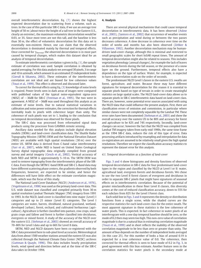
The SIR-C data analyzed in this study is fully polarimetric. Theresults presented in Figs. 3 and 4 are from the HH-HH polarization, i.e.transmission and reception of horizontally polarized waves for bothpasses. Fig. 5 shows the coherence statistics of HH-HH and VV-VVpolarizations for the four land-cover classes discussed so far. Thedifference in temporal decorrelation between land-cover classes forboth polarizations is quite apparent here. Agricultural land suffers theleast amount of temporal decorrelation in either polarization, asevident by the fact that histograms of this land-cover class are morebiased toward unity than any other class. As a scalar measure of theamount of temporal decorrelation, one can consider the mode of eachdensity function. The distribution mode for interferometric coherencein agricultural land lies between 0.96 and 9.97 for the two polari-zations while mode of coherence for pixels from forested terrain isbetween 0.82 and 0.84.

Figs. 6 and 7 show observed correlation statistics for the four mainpolarizations.Water pixels in the cross-polarization data seem to have

0 0.5 1

0 0.5 1

0

1

2

3

4

Occ

uran

ce (

%)

0

1

2

3

4

Occ

uran

ce (

%)

Correlation Magnitude

Fig. 5. Coherence statistics, density (left) and distribution (right) functions of four land-clasthe polarizations HH-HH, and VV-VV. These statistics include pixels from the entire swath.

high coherence. This is the effect of particularly low SNR for cross-polarization data compared to co-polarized data over water, and maybe suggestive of imaging ambiguities which are normal but typicallyinsignificant in regions with higher reflected power. Vertical polar-ization data seems to be better correlated than data from horizontalpolarization in agricultural areas while the opposite can be seen foreither of the forest classifications, an interesting if not slight signature,that may warrant future investigation.

4.2. Extent of atmospheric effects on interferometric coherence

The large scale statistics seen in Figs. 3–7 are inclusive of pixelsfrom all the area mapped by this SIR-C swath. The statistics areinclusive of pixels that may or may not have variations resulting fromweather events or other phenomenon discussed in Section 4.1. Coher-ence statistics from some individual scenes in Figs. 3 and 4 exhibitdeviations from the mean behavior. The density functions of southernscenes 52102 to 52108 for forests have significant contributions fromlow correlation pixels. Scene 52102 in particular (marked in Figs. 3and 4 by the thicker dark blue line) has a near bimodal distribution forforested areas, indicating a high concentration of decorrelated pixels.An inspection of the scene shows patterns of aweather event apparentfrom a sharp gradient in coherence across the scene. Similar patternsare observed from scenes 52104 to 52108, though they are not aspronounced. On the other hand, there is very high coherence innorthern scenes, particularly 52126 (in Figs. 3 and 4 this is representedby the cyan linewith dottedmarkers)withmean coherences as high as0.92 for forested areas.

To further investigate the effects of weather phenomenon, thecoherence for agricultural and forested areas along the entire SIR-Cswath was analyzed as a function of latitude. The result is shown inFig. 8. Each point on this curve is the averaged correlation magnitudeof forested or agricultural land for strips of 100 cross-track InSAR lines,representing roughly 9600 ha for each point and plotted as a functionof the latitude measured at the center of each strip. To assure that the

0 0.5 1

0 0.5 1

0

20

40

60

80

100

Hec

tare

s (%

)

0

20

40

60

80

100

Hec

tare

s (%

)

Correlation Magnitude

AgricultuerDeciduousEvergreenWater

ses, water, agricultural area, deciduous and evergreen forest are plotted as a function ofDifferences between these distributions are statistically significant.

0 0.5 1 0 0.5 10

1

2

3

4

Water

Occ

uran

ce (

%)

0

1

2

3

4

Occ

uran

ce (

%)

0

1

2

3

4

Occ

uran

ce (

%)

0

1

2

3

4

Occ

uran

ce (

%)

Agriculture

0 0.5 1

Evergreen forest

Correlation Magnitude0 0.5 1

Correlation Magnitude

Deciduous forest

HH−HHVV−VVHV−HVVH−VH

Fig. 6. Probability density functions of coherence obtained from pixels from the entire SIR-C swath are shown for four different land-classes (water, agricultural land, evergreen anddeciduous forests) and four polarizations (HH-HH, VV-VV, HV-HV, VH-VH). Agricultural land is better correlated in VV-VV polarization, while forested areas seem to have bettercoherence for HH-HH polarization.

2893R. Ahmed et al. / Remote Sensing of Environment 115 (2011) 2887–2896

averaged coherence value per strip is representative, mean valueswere not considered for sample populations of less than 50 ha (200samples) for each land-cover classification. This was particularlynecessary for strips dominated by water.

0 0.5 10

20

40

60

80

100Water

Hec

tare

s (%

)

0

20

40

60

80

100

Hec

tare

s (%

)

0 0.5 1

Evergreen forest

Correlation Magnitude

Fig. 7. Distribution functions of coherence are shown for four land-classes and four polaAbnormally high coherence in water pixels for these polarizations is explained by lack of S

The first thing to notice in Fig. 8 is that irrespective of latitude thereis always some amount of temporal decorrelation for either land-covertype. Secondly, agricultural areas almost always suffered less temporaldecorrelation than forests. The difference seen between mean

0 0.5 10

20

40

60

80

100

Hec

tare

s (%

)

0

20

40

60

80

100

Hec

tare

s (%

)

Agriculture

0 0.5 1

Correlation Magnitude

Deciduous forest

HH−HHVV−VVHV−HVVH−VH

rizations. Difference between HV-HV and VH-VH pixels is statistically insignificant.NR.

36 37 38 39 40 41 42 43 44 45

0.4

0.5

0.6

0.7

0.8

0.9

1

Latitude (deg)

Cor

rela

tion

Mag

nitu

de

ForestsCrops

Active precipitationduring pass 2

high winds

Peak fall colors occur in midOctober

Peak fall colors occur in earlyNovember

Fig. 8. Correlation magnitude of agricultural and forested land is plotted as a function of latitude. Each point represents mean coherence of respective pixels from 100 cross-trackInSAR lines. Weather and seasonal events such as active precipitation, high winds and fall foliage times are annotated.

2894 R. Ahmed et al. / Remote Sensing of Environment 115 (2011) 2887–2896

coherence for each land-cover class is statistically significant at almostevery latitude except for the points from the very last scene 52126(around 45° latitude). There also seems to be a general upward trendin coherence as a function of latitude, with the highest coherence seenfarthest north. The highest temporal decorrelation is seen at lowerlatitudes, as much as 70% at one point.

As discussed earlier, and indicated in Fig. 8, the reasons for such hightemporal decorrelation at lower latitudes could be weather events. Thesharp gradient visible in coherence scene 52102, shows up as a suddenjump in coherence at a latitude of 36°. This latitude is at the center ofscene 52102. Although the severity of temporal decorrelation dependson land-cover class, the similarity in trends for both classifications also

10th October

Fig. 9. Hourly precipitation leading up to pass 2 with zero indicating the actual time of SIR-Cdot represents a station that reported some amount of precipitation during this time. The cobefore the shuttle overpass, i.e. 5 pm on the 9th, black represents rain at 3 am on the 10th)

points toward aweather event as a possible source of this decorrelation.Similarly, between 37° and 39° of latitude there appears a region ofincreased decorrelation, where the amount of decorrelation peaks near40%, and seems to correspond to gradients observed in scenes 52104 to52108.

The weather events that may have caused this decorrelation over ashort period of 24 h are likely precipitation and high winds. Toinvestigate further we look at the NCDC archives of hourly surfaceclimatological data from some 1500 weather stations in relativeproximity to the area mapped by this swath. Hourly precipitation andwind data collected around the time of the SIR-C overpass from thesestations was analyzed and presented in Figs. 9 and 10. Fig. 9 shows

(pass 2)

0

1

2

3

4

5

6

7

8

9

10hrs

overpass (3 am on the 10th). The radar swath is approximated by the red polygon, eachlor of each dot represents time before the second pass (white is precipitation ten hours.

Pass 2

Pass 1

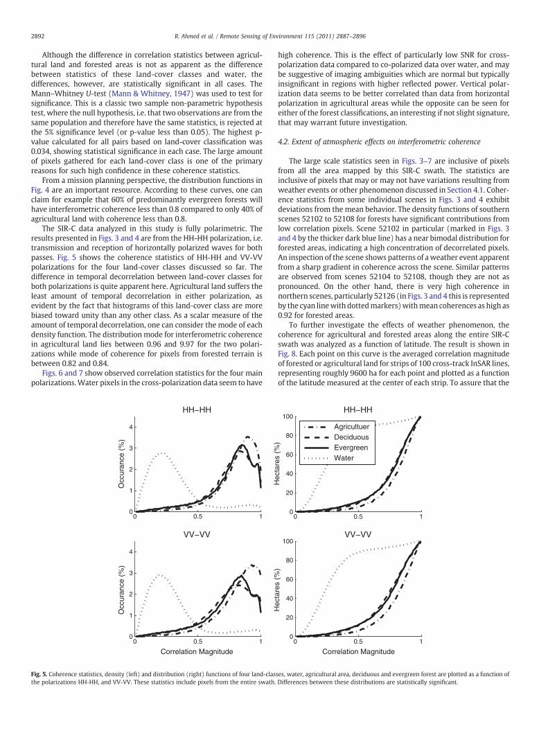
Fig. 10. Wind data from weather stations for the two shuttle passes over the eastern US is plotted. Radar swath is approximated by the gray polygon. Difference between times atwhich wind is measured at the weather stations and SIR-C shuttle overpass is around 3 min. Arrow length indicates wind speed with the largest arrow representing a speed ofaround 14 m/s.

2895R. Ahmed et al. / Remote Sensing of Environment 115 (2011) 2887–2896

precipitation data from weather stations for the second pass of SIR-C.In the figure, a solid red polygon approximates the SIR-C swath, andeach circle represents the weather station that reported a non trivialamount (more than 0.5 mm/h) of precipitation. The color of each circlerepresents how many hours before the second SIR-C pass that thestation recorded precipitation. White, for example represents precip-itation 10 h before the second pass while a black dot representsprecipitation observed at the time of the second SIR-C overpass. Noprecipitation is reported up to 12 h before the first SIR-C data take onOctober 9th from weather stations surrounding the swath in theeastern U.S. One can see from Fig. 9 that a large weather systemdevelops around 2 pm (EST) on the 9th (12 h prior to the second datatake) and moves northeast with some stations reporting moderaterain (up to 8 mm/h). By the time of the second data take (3 am EST onthe 10th) most of the area around the SIR-C swath has no activeprecipitation except at the very southern tip. The amount ofprecipitation recorded by weather stations in this region at this timeis fairly high, up to 13 mm/h, indicative of moderate to heavy rainfall.Hence, these results show that the high temporal decorrelation seen inFig. 8 around 36° is very likely to be caused by active precipitation.

Similarly, wind data at the time of both the SIR-C overpasses isanalyzed and plotted in Fig. 10. Highwinds are seen between latitudes37° and 39°, sometimes as high as 14 m/s. These winds are strongenough to cause branches to move, and may be the reason for thedecorrelation seen in Fig. 8 for this range of latitudes.

The northern most scene (pr52126) is characterized by lowtemporal decorrelation, only about 8%. There is a lack of wind andprecipitation for this area at the time of the SIR-C overpasses. Asindicated on Fig. 8, peak fall color and leaf drying occurs sometimeduring mid-October for latitudes 43° and above with leaf-offconditions occurring two weeks later. Hence, in the northern-mostregion, most deciduous trees would be either dry or in leaf-offconditions. Temperatures for the Washington county (the location ofscene) weather stations at the time of SIR-C overflight suggesttemperature ranges between 40° and 50 °F. A combination of stableweather conditions and dry or no leaves on deciduous forests seem alikely contributor for the low values of temporal decorrelation.

5. Conclusions

In this study a large region, more than a million hectares, over theeastern United States is analyzed using SIR-C L-Band InSAR data. Smallperpendicular baselines allowed analysis of temporal decorrelationeffects. The National Land Classification Dataset (NLCD) was used tocreate large scale statistics of temporal decorrelation for various land-cover types in the form of probability density, and distributionfunctions. These statistics can prove to be useful form amission designstandpoint as an indication of the amount of temporal decorrelationthat might be typically expected for a short repeat-pass InSARmission. Results showed that some amount of temporal decorrelationis present throughout the data, that it varies with land-cover type andthat the degree of temporal decorrelation is likely weather (precip-itation and wind) and seasonally (i.e. phenology and cultivationcycles) dependent. Active precipitation seems to cause up to 70% lossin coherence, wind also seems to decrease coherence, although by notas much. Stable weather and fall foliage conditions might havecontributed to high coherence seen in northern latitudes.

References

Anderson, J., Hardy, E., Roach, J., & Witmer, R. (1976). A land use and land coverclassification system for use with remote sensor data. U.S. Geological Survey Prof.Paper 964 (pp. 28).

Askne, J. I. H., Dammert, P. B. G., Ulander, L. M. H., & Smith, G. (1997). C-band repeat-pass interferometric SAR observations of the forest. IEEE Transactions on Geoscienceand Remote Sensing, 35(1).

Askne, J., Santoro, M., Smith, G., & Fransson, J. (2003). Multitemporal repeat-pass SARinterferometry of boreal forests. IEEE Transactions on Geoscience and RemoteSensing, 41, 1540–1550.

Cloude, S. R. (2006). Polarization coherence tomography. Radio Science, 41(4).Cloude, S. R., & Papathanassiou, K. P. (1998). Polarimetric SAR interferometry. IEEE

Transactions on Geoscience and Remote Sensing, 36(5), 1551–1565.Dobson, M. C., Ulaby, F. T., Toan, T. L., Beaudoin, A., Kasischke, E. S., & Christensen, N.

(1992). Dependence of radar backscatter on coniferous biomass. IEEE Transactionson Geoscience and Remote Sensing, 30(2), 412–415.

Farr, T., Rosen, P. A., Caro, E., Crippen, R., Duren, R., Hensley, S., et al. (2007). The shuttleradar topography mission. Review of Geophysics, 45.

Freeman, A., Alves, M., Chapman, B., Cruz, J., Kim, Y., Shaffer, S., et al. (1995). SIR-C dataquality and calibration results. IEEE Transactions on Geoscience and Remote Sensing,33(4), 848–857.

2896 R. Ahmed et al. / Remote Sensing of Environment 115 (2011) 2887–2896

Gesch, D., Oimoen, M., Greenlee, S., Nelson, C., Steuck, M., & Tyler, D. (2002). The NationalElevation Dataset. Photogrammetric Engineering and Remote Sensing, 68, 5–11.

Gierull, C., & Sikaneta, I. C. (2002). Estimating the effective number of looks ininterferometric SAR data. IEEE Transactions on Geoscience and Remote Sensing, 40(8),1733–1742.

Guttman, N., & Quayle, R. (1996). Historical perspective of the U.S. climate divisions.Bulletin of the American Meteorological Society, 77, 293–303.

Hagberg, J. O., Ulander, L. M. H., & Askne, J. (1995). Repeat-pass SAR interferometry overforested terrain. IEEE Transactions on Geoscience and Remote Sensing, 33(2).

Imhoff, M. L. (1995). Radar backscatter and biomass saturation: Ramifications for globalbiomass inventory. IEEE Transactions on Geoscience and Remote Sensing, 33(2).

Kellendorfer, J., Walker, W. S., Pierce, L. E., Dobson, C., Fites, J. A., Hunsaker, C., et al.(2004). Vegetation height estimation from shuttle radar topography mission andnational elevation datasets. Remote Sensing of the Environment, 93, 339–358.

Le Toan, T., Beaudoin, A., Riom, J., & Guyon, D. (1992). Relating forest biomass to SARdata. IEEE Transactions on Geoscience and Remote Sensing, 30(2), 403–411.

Li, F., & Goldstein, R. M. (1990). Studies of multibaseline spaceborne interferometricsynthetic aperture radars. IEEE Transactions on Geoscience and Remote Sensing, 28,88–98.

Mann, H., & Whitney, D. (1947). On a test of whether one of two random variables isstochastically larger than the other. Annals of Mathematical Science, 18(1), 50–60.

National Research Council (Ed.) (2007), Earth science and applications from space:National imperatives for next decade and beyond, National Academic Press,Washington, D.C.

Papathanassiou, K. P., & Cloude, S. R. (2001). Single-baseline polarimetric SARinterferometry. IEEE Transactions on Geoscience and Remote Sensing, 39(11),2352–2363.

Papathanassiou, K., & Cloude, S. R. (2003). The effect of temporal decorrelation oninversion of forest parameters from Pol-InSAR data. Proc. of IEEE InternationalGeoscience and Remote Sensing Symposium., 3 (pp. 1429–1431).

Rodriguez, E., & Martin, J. M. (1992). Theory and design of interferometric syntheticaperture radars. Proceedings of the Institution of Electrical Engineers, 139(2), 147–159.

Rosen, P., Hensley, S., Joughin, I. R., Li, F. K., Madsen, S. N., Rodriguez, E., et al. (2000).Synthetic aperture radar interferometry. Proceedings of the Institution of ElectricalEngineers, 88(3), 333–382.

Santoro, M., Askne, J., Smith, G., & Fransson, J. (2002). Stem volume retrieval in borealforests from ERS-1/2 interferometry. Remote Sensing of Environment, 81, 19–35.

Santoro, M., Shvidenko, A., McCallum, I., Askne, J., & Schmullius, C. (2007). Properties ofERS-1/2 coherence in the Siberian boreal forest and implications for stem volumeretrieval. Remote Sensing of the Environment, 106, 154–172.

Simard, M., Zhang, K., Rivera-Monroy, V., Ross, M., Ruiz, P., Castaneda-Moya, E., et al.(2006). Mapping height and biomass of mangrove forests in everglades nationalpark with SRTM elevation data. Photogrammetric Engineering and Remote Sensing,72(3), 299–311.

Stehman, S., Wickham, J., Smith, J., & Yang, L. (2003). Thematic accuracy of the 1992national land-cover data for the eastern United States: Statistical methodology andregional results. Remote Sensing of Environment, 86, 500–516.

Touzi, R., Lopez, A., Bruniquel, J., & Vachon, P. W. (1999). Coherence estimation for SARimagery. IEEE Transactions on Geoscience and Remote Sensing, 37(1), 135–149.

Treuhaft, R. N., & Cloude, S. R. (1999). The structure of oriented vegetation frompolarimetric interferometry. IEEE Transactions on Geoscience and Remote Sensing,37(5), 2620–2624.

Treuhaft, R., Madsen, S., Moghaddam, S., & Zyl, J. V. (1996). Vegetation characteristics andunderlying topography from interferometric radar. Radio Science, 31, 1449–1485.

Treuhaft, R., & Siqueira, P. (2000). Vertical structure of vegetated land surfaces frominterferometric and polarimetric radar. Radio Science, 35(1), 141–177.

Vogelmann, J., Sohl, T., Campbell, P., & Shaw, D. (1998). Regional land covercharacterization using LANDSAT thematic mapper data and ancillary data sources.Environmental Monitoring and Assessment, 51, 415–428.

Walker, W., Walker, W., & Pierce, L. E. (2007). Quality assessment of SRTM C- and X-band interferometric data: Implications for the retrieval of vegetation canopyheight. Remote Sensing of the Environment, 106, 428–448.

Wu, S. T. (1987). Potential application of multi-polarization SAR for plantation pinebiomass estimation. IEEE Transactions on Geoscience and Remote Sensing, GRS-25,403–409.

Zebker, H. A., & Villasenor, J. (1992). Decorrelation in interferometric radar echoes. IEEETransactions on Geoscience and Remote Sensing, 30, 950–959.