Journal of

Marine Science and Engineering

Article

A Study on the Effectiveness of the Heading Control on theMooring Line Tension and Position Offset for an Arctic FloatingStructure under Complex Environmental Loads

Hyun Hwa Kang 1 , Dae-Soo Lee 1 , Ji-Su Lim 1, Seung Jae Lee 1, Jinho Jang 2 , Kwang Hyo Jung 3

and Jaeyong Lee 4,*

�����������������

Citation: Kang, H.H.; Lee, D.-S.; Lim,

J.-S.; Lee, S.J.; Jang, J.; Jung, K.H.; Lee,

J. A Study on the Effectiveness of the

Heading Control on the Mooring Line

Tension and Position Offset for an

Arctic Floating Structure under

Complex Environmental Loads. J.

Mar. Sci. Eng. 2021, 9, 102. https://

doi.org/10.3390/jmse9020102

Received: 22 December 2020

Accepted: 11 January 2021

Published: 20 January 2021

Publisher’s Note: MDPI stays neutral

with regard to jurisdictional claims in

published maps and institutional affil-

iations.

Copyright: © 2021 by the authors.

Licensee MDPI, Basel, Switzerland.

This article is an open access article

distributed under the terms and

conditions of the Creative Commons

Attribution (CC BY) license (https://

creativecommons.org/licenses/by/

4.0/).

1 Division of Naval Architecture and Ocean Systems Engineering, Korea Maritime and Ocean University,Busan 49112, Korea; khh20160653@gmail.com (H.H.K.); danelee2601@naver.com (D.-S.L.);20140571@kmou.ac.kr (J.-S.L.); slee@kmou.ac.kr (S.J.L.)

2 Ice-Covered Waters Engineering Research Center, Korea Research Institute of Ships and Ocean Engineering,Daejeon 34103, Korea; jangj@kriso.re.kr

3 Department of Naval Architecture and Ocean Engineering, Pusan National University, Busan 46241, Korea;kjung@pusan.ac.kr

4 Department of Naval Architecture and Ocean Engineering, Dong-eui University, Busan 47340, Korea* Correspondence: jlee@deu.ac.kr; Tel.: +82-51-890-2596

Abstract: Even though interest in developing the Arctic region is increasing continuously, the stan-dard procedure to be used to analyze the station-keeping performance of a floater consideringice loads has not been established yet. In this paper, the effectiveness of heading control with adynamic positioning system is analyzed to evaluate the improvement of the performance of thestation-keeping system in the ice conditions. Complex environmental loads with ice-induced forceswere generated and applied to a ship type floater with dynamic positioning and mooring systems.Three-hour time-domain simulations were conducted for the two different station-keeping systemswith mooring only and mooring with a dynamic positioning system. Position offsets and mooringline tensions for the two scenarios were compared with maximum values and most probable maxima(MPM) values. The results of the simulation showed that the heading control can reduce 8.2% ofMPM values for the mooring lines and improve the station-keeping performance by about 16.3%.The validity of the station-keeping system that was designed was confirmed, and it is expected thatthe specification of mooring lines can be relaxed with the heading control.

Keywords: station-keeping system; dynamic positioning (DP); dynamic positioning assisted mooring(DPAM); most probable maximum (MPM); maximum breaking load (MBL); ice load; heading control;mooring line

1. Introduction

Floating offshore structures must have station-keeping capability to conduct therequested work in stable conditions. The position of a floating-type production platform isrequired to be within 10% of the installed water depth for the safety of risers. Generally,mooring systems and dynamic positioning (DP) systems are used for the station-keeping offloating structures. Two types of mooring systems have been used extensively, i.e., spreadmooring and single point mooring with turret. Turret systems commonly are installedin severe environments. In the Arctic region, the ice induced load must be considered indesigning a station-keeping system.

One of the most serious problems for a turret system in ice conditions is the difficultyin weathervaning, which is the main advantage of the system. The turret makes the floateralign with the direction of the significant environmental load. However, when the attackangle of the ice field is over a certain range, the restoration force is not enough to rotate,

J. Mar. Sci. Eng. 2021, 9, 102. https://doi.org/10.3390/jmse9020102 https://www.mdpi.com/journal/jmse

J. Mar. Sci. Eng. 2021, 9, 102 2 of 17

and the floater begins to drift in the direction that the ice field is moving. This results inexcessive tension on the mooring lines, and they may break [1].

To prevent this situation, either a DP assisted mooring (DPAM) system or a thruster-assisted mooring (TAM) system can be used. DPAM has been used in severe environmentsfor station-keeping purposes. Ice conditions are one such environment, and DPAM can beconsidered as a solution. Thrusters can give enough moment to turn the floating structureto the direction of the wind or the directions of other significant forces. This leads to thereduction of the tension in the mooring lines.

In designing DPAM, the designs of the mooring line and the DP system are con-sidered at the same time. There are two main approaches in designing a mooring sys-tem, i.e., the static frequency-domain approach and the dynamic time-domain approach.The frequency-domain analysis has advantages in time and the possible combination ofvarious environmental conditions. These characteristics are useful in the initial basic de-sign stage. However, due to the limitation of the accuracy of nonlinear coupled analysis,the time-domain analysis also must be conducted [2]. After the analyses of the equilibriumposition analysis and the linear frequency response, variations in the tension of the mooringlines are monitored in a time-domain analysis. The results are used to predict the fatiguedamage during the design life and to decide the final arrangement of the mooring line [3].The performance of DPAM in the time domain can be evaluated by observing the offset ofthe position and monitoring the variation in the tension of the mooring line. The location ofthe floater must be within the allowable radius, and the statistically processed tensions onthe designed mooring lines must be less than 60% of the maximum breaking load (MBL) [4].The previous research on the station-keeping of a floater in the Arctic region is inadequatefor considering complex environmental loads that include ice forces as well as the loadsassociated with the wind, waves, and currents.

In the time domain, the station-keeping performance considers the operational andsurvival conditions in which the designed structure will be operated. The wind, current,and wave conditions are defined well in the many rules and standards of the classificationsocieties. However, to date, evaluation methods and design standards that consider theice load have not been provided. The most difficult thing in considering the ice load is toassess the effect of the load on the station-keeping performance.

There are three major methods that are used to evaluate the station-keeping perfor-mance in ice-covered waters, i.e., on-site operations, ice tank tests, and computer simula-tions. In 2004, the International Ocean Drilling Program (IODP) conducted 302 arctic coringexpedition, and collected data concerning the difficulties associated with maintaining agiven position in the ice [5–7]. As a part of the project entitled dynamic positioning in icecondition, i.e., the DYPIC project, a model test was conducted for an Arctic drilling vesselin 2014 [8,9]. In addition, Canada’s National Research Council (NRC) also conducted anice tank test for a drilling vessel [10]. However, these on-site tests and ice tank tests areexpensive and have limitations when it comes to changing the test conditions.

To overcome these limitations, there are active research programs related to the sim-ulation of ice–structure interactions. The numerical methods generally use the discreteelement method (DEM), and simulations are being conducted on station-keeping in ice con-ditions, ice-structure interactions, and the navigation of ships in ice-covered waters [11–13].To reduce the time required for the simulations, researchers used the graphical process-ing unit (GPU) to develop the GPU event mechanics (GEM) for use in acquiring a goodfloating-point calculation [14,15]. Such software still has limitations, i.e., the direction inwhich the ice is drifting cannot be changed, and other environmental loads, such as thewave load, have not been incorporated in the program.

Recently, ice load generation methods that consist of complex environmental loadshave been suggested for the evaluation of station-keeping performance in the time domain.In [16], an ice load generation method was proposed by combining the mean values of theice load from the ice tank test and the spectrum values from GEM. Another similar method

J. Mar. Sci. Eng. 2021, 9, 102 3 of 17

that generates ice forces on the structure at an arbitrary heading angle was introduced foruse in the time-domain analysis [17].

This paper is focused on the evaluation of the station-keeping performance of afloating production structure using the ice load generation module. The DP system isadded for the heading control to the mooring system, and simulations are conducted toappraise the effectiveness of the DP system. A complex environmental condition was set byconsidering the target site. Then, time-domain simulations are conducted for two scenarios,i.e., mooring only and DPAM. The results are processed, and the effectiveness of the DPAMis examined over the mooring system. The rest of the paper is organized as follows.

The fundamentals in analyzing the performance of the station-keeping are summa-rized in Section 2. The third section describes the information about the target floater,the ice load generation module, and settings for the time-domain simulation. The resultsare reviewed in Section 4. The variations of the position offset and mooring tension areobserved, and the performance was evaluated using the most probable maxima values. Theresults are summarized in Section 5, and the advantage of the heading control is described.Additionally, the limitations of the research and future works are discussed.

2. Dynamics in Ice Condition and Procedure to Evaluate the Station-KeepingPerformance2.1. Frequency-Domain Analysis

An analysis of the motion of an offshore floater is to get a solution of the Laplaceequation, which is composed of velocity potentials. The pressure acting on the surface ofthe floater in a fluid field is derived from the following Equation (1):

PFluid = −ρgz− ρ∂Φ∂t

= −ρgz− ρ

(∂ΦI∂t

+∂ΦD

∂t+

∂ΦR∂t

)= PStatic + PF.K. + PD + PR, (1)

where ρ is the density of water, g is the gravitational acceleration, z is the depth, and t is thetime. ΦI , ΦD, ΦR are the incident, diffraction, and radiation potentials, respectively. In therightmost term, PStatic is the static pressure, PF.K. is the Froude–Krylrov pressure, PD is thediffraction pressure, and PR is the radiation pressure. By integrating the pressure for theentire submerged area of the floater, the pressure terms in Equation (1) can be converted toforces and expressed as Equation (2) by Newton’s law of motion.

M..x = FGravity + Fstatic + FF.K. + FD + FR (2)

After calculating hydrostatic and hydrodynamic coefficients with the incident anglesand frequencies of the waves acting on the structure, the motion ratio amplitude operator(RAO) of the floater is computed in the frequency-domain analysis. The results are used toevaluate the motion characteristics of the floater designed to be operated at the target site.

2.2. Time-Domain Analysis

Since the floater was modeled and designed as a linear system, the characteristicsof the nonlinear elements are not represented well in the frequency-domain analysis.To resolve these limitations, time-domain analysis is required [18]. Generally, the equationof motion for a floater can be expressed as shown in Equation (3) for the time-domainanalysis.

M..x = −Kx + Fexciting − A

..x− C

.x + FExternal (3)

For a floater with mass M, FGravity is the body force, and Fstatic, FF.K, FD, and FRare the surface forces by the fluid. FGravity and Fstatic compose the restoration force (Kx).FF.K and FD are wave excitation forces (Fexciting). The radiation force, FR, is composed ofmass and damping terms (FR = −A

..x − B

.x), where A is the added mass, and B is the

damping coefficient. FExternal means all other environmental forces in the Arctic region,which include wind, current, and ice loads. After transpositioning the added mass term,

J. Mar. Sci. Eng. 2021, 9, 102 4 of 17

the damping and restoration terms on the right side of Equation (3) can be expressed asshown in the following Equation (4):

(M + A)..x + C

.x + Kx = Fexciting + Fwind + Fcurrent + FDP + Fmooring + Fice (4)

where Fwind, Fcurrent, and Fice denote the wind, current, and ice forces, respectively. FDP andFmooring are the forces by the station-keeping system with DP and mooring.

2.3. Forces by the Station Keeping System2.3.1. Force by the DP System

Generally, PID control logic is used for a DP system on a floating offshore structure.Figure 1 shows the general form of a DP control system. The logic uses the error and therate of change of the error from the target state (ηd) and the current state (ηa). Consideringthe proportional gain (KP), derivative gain (Kd), and integral gain (Ki), the required thrustcan be derived from the following Equation (5):

τre f (t) = KPε(t) + KI

∫ t

0ε(τ)dτ + KD

.ε(t) (5)

J. Mar. Sci. Eng. 2021, 9, x FOR PEER REVIEW 4 of 18

damping and restoration terms on the right side of Equation (3) can be expressed as shown in the following Equation (4): (𝑀 + 𝐴)𝑥 + 𝐶𝑥 + 𝐾𝑥 = 𝐹 + 𝐹 + 𝐹 + 𝐹 + 𝐹 + 𝐹 (4)

where 𝐹 , 𝐹 , and 𝐹 denote the wind, current, and ice forces, respectively. 𝐹 and 𝐹 are the forces by the station-keeping system with DP and mooring.

2.3. Forces by the Station Keeping System 2.3.1. Force by the DP System

Generally, PID control logic is used for a DP system on a floating offshore structure. Figure 1 shows the general form of a DP control system. The logic uses the error and the rate of change of the error from the target state (𝜂 ) and the current state (𝜂 ). Considering the proportional gain (𝐾 ), derivative gain (𝐾 ), and integral gain (𝐾 ), the required thrust can be derived from the following Equation (5): 𝝉 (𝑡) = 𝐾 𝜀(𝑡) + 𝐾 𝜀(𝜏) 𝑑𝜏 + 𝐾 𝜀(𝑡) (5)𝐹 , , 𝐹 , , and 𝑀 , are the forces required to restore the surge, sway, and yaw mo-tion of the floater. Then, the required thrust can be summarized as shown in Equation (6): 𝝉 = [𝐹 , , 𝐹 , , 𝑀 , ] (6)

Figure 1. General form of a dynamic positioning (DP) control system.

For a DP system with n thrusters, the thrust vector for each propulsion system can be expressed as follows: 𝒖 = (𝑢 , , 𝑢 , ), (7)

where 𝑢 , and 𝑢 , are the forces of the ith propulsion system acting in the x-direction and y-direction in the body-fixed coordinate. The moment is calculated based on the cen-ter of gravity (𝑥 , 𝑦 ) and the locations of the thruster (𝑥 , 𝑦 ), i.e.,: 𝐿 , = 𝑥 − 𝑥 , 𝐿 , = 𝑦 − 𝑦 .

(8)

Forces on the floater by 𝑢 can be summarized as: 𝐹 , = 𝑢 , , 𝐹 , = 𝑢 , , 𝑀 , = 𝐿 , 𝑢 , − 𝐿 , 𝑢 , ,

(9)

Figure 1. General form of a dynamic positioning (DP) control system.

Fx,re f , Fy,re f , and Mz,re f are the forces required to restore the surge, sway, and yawmotion of the floater. Then, the required thrust can be summarized as shown in Equation (6):

τre f =[

Fx,re f , Fy,re f , Mz,re f

]T(6)

For a DP system with n thrusters, the thrust vector for each propulsion system can beexpressed as follows:

ui =(ui,x , ui,y

), (7)

where ui,x and ui,y are the forces of the ith propulsion system acting in the x-direction andy-direction in the body-fixed coordinate. The moment is calculated based on the center ofgravity (xCoG, yCoG) and the locations of the thruster (xCoG, yCoG), i.e.,:

Li,x = xi − xCoG,Li,y = yi − yCoG. (8)

Forces on the floater by ui can be summarized as:

Fi,x = ui,x,Fi,y = ui,y,Mi,z = Li,xui,y − Li,yui,x, (9)

J. Mar. Sci. Eng. 2021, 9, 102 5 of 17

which can be formularized as the following; 1 00 1−Li,y Li,x

[ ui,xui,y

]=

Fi,xFi,yMi,z

↔ Biui = Fi (10)

To keep the floater at the desired position, n thrusters are required to generate therequired thrust, as shown in Equation (11):

Bu = τre f (11)

whereB = [B1 . . . Bi . . . Bn], u = [u1 . . . ui . . . un]

T (12)

The Lagrange multiplier method is the most popular method for the allocation of thethrust for each propulsion system, and it can be stated as follows:

minu

uTWu s.t.Bu = τre f (13)

where W is the weight matrix (W ∈ R2n×2n, B ∈ R3×2n and u ∈ R2n). Using the Karush–Kuhn–Tucker (KKT) conditions provides the following optimal solution:

u = W−1BT(

BW−1BT)−1

τre f (14)

2.3.2. Force by the Mooring Lines

For a motion analysis in the time domain, mooring lines are modeled with the lumpedmass method or the Morison elements method. In this paper, the Morison elements methodis used to consider the drag force. As shown in Figure 2a, a mooring line is assumed tobe the combination of circular slender cylinders [19]. Figure 2b shows the hydrodynamic

force (⇀Fh), inertial load (

⇀W), and structural loads (

→T ,→V,

→T) that are applied to each

element (cylinder). ∇Se and De are the length and diameter of the cylinder, respectively.Each element has two nodes, i.e., one at the anchor side (first node) and one at the floater

side (second node). At the first node,→T is the tension vector,

→M is the bending moment

vector, and→V is the shear force vector. Then, the equation of motion for the circular cylinder

can be expressed as:

∂→T

∂se+

∂→V

∂se+

⇀W +

⇀Fh = m

∂2→R

∂t2∂→M

∂se+

∂→R

∂se×→V = −→q (15)

where m is the mass per unit length,→q is the distributed moment, and

→R is the posi-

tion vector. Hydrodynamic force is the combination of buoyance force, drag force, andthe acceleration terms at nodes Nj and Nj+2 with added mass, and it can be expressedas follows:

Fh = Fb + Fd −ma

[→a j,→a j+2

]T(16)

where ma

[→a j,→a j+2

]Tis the radiation force. The buoyance force is expressed as:

Fb =

{0, 0,

12

ρw AcjLjg, 0, 0,12(ρw AcjLj + Mb)g

}T(17)

where ρw is the density of water, Acj is the cross-sectional area at jth node, Lj is the lengthof the jth element, and Mb is the mass of the displaced water. Drag force is expressed in

J. Mar. Sci. Eng. 2021, 9, 102 6 of 17

terms of the relative velocity between the current velocity (Uj+1) and the element (Vj+1),drag coefficient and projected area, as follows:

Fd(t) =

{fd(j)

fd(j + 1)− 12 CdbSbρw

∣∣Uj+1(t)−Vj+1(t)∣∣{Uj+1(t)−Vj+1(t)

} } (18)

J. Mar. Sci. Eng. 2021, 9, x FOR PEER REVIEW 6 of 18

𝐹 (𝑡) = 𝑓 (𝑗)𝑓 (𝑗 + 1) − 12 𝐶 𝑆 𝜌 𝑈 (𝑡) − 𝑉 (𝑡) 𝑈 (𝑡) − 𝑉 (𝑡) (18)

(a) (b)

Figure 2. (a) Model of a dynamic mooring line; (b) free body diagram for a Morison element.

2.4. Ice-Induced Load The ice-induced load on the structure is related to mass and acceleration. To calculate

the load, the direction of the ice drift and the angle of attack must be determined. Accord-ing to the research associated with the long-term tracking of ice, the movement is influ-enced by both the wind and currents [20]. Generally, the acceleration of the pack ice is determined by the items such as the velocity of the ice, the Coriolis parameter, the air–ice drag acceleration, and the water–ice drag acceleration. The air–ice drag acceleration is computed based on the wind speed, the density of the seawater, the density of air, and the air–ice drag coefficient. The velocity of the current, the thickness of the ice, the density of the seawater, and the water–ice drag coefficient are considered for the water–ice drag coefficient.

The drift direction of an ice pack is regarded to be similar to the direction of the cur-rent. Sensors were installed on the ice flow, and the metocean data were compared with the movement of the ice. However, the wind effect must be considered in designing a floating offshore structure because the severe wind is one of the key causes of the motion of a vessel. Therefore, in this research, the drift of the ice is assumed to be influenced by both the wind and the current. The ice load is generated from the experimental data from the ice tank, and it is used in the analysis of the motion in the time domain. In the ice tank test, a model floater is towed while being restrained for 6D movement, and the resistance forces are measured. For this research, experiments were repeated for nine different head-ing angles at 10° intervals from −40° to 40° at the ice tank of the Korea Research Institute of Ships and Ocean Engineering (KRISO). The data were post-processed with the statisti-cal method, and the ice load was calculated at an arbitrary heading angle in the time-domain simulation. This method cannot precisely represent the motion of a floater in an actual ice-covered sea with a large initial heading angle. However, meaningful results can be derived if the heading is kept within small angles, as was carried out in this research.

2.5. Procedure for the Statistical Analysis on the Performance The mooring system that was designed is evaluated by observing the tension on the

mooring lines and the offset of the position. Tension is generally observed at the fairlead and the anchor. However, simulation results for the maximum line tension on the moor-ing lines and the position offset have different values based on the seed number of irreg-ular waves used in the 3-h simulation [4,21,22]. The decision to judge whether the system

Figure 2. (a) Model of a dynamic mooring line; (b) free body diagram for a Morison element.

2.4. Ice-Induced Load

The ice-induced load on the structure is related to mass and acceleration. To calculatethe load, the direction of the ice drift and the angle of attack must be determined. Accordingto the research associated with the long-term tracking of ice, the movement is influenced byboth the wind and currents [20]. Generally, the acceleration of the pack ice is determined bythe items such as the velocity of the ice, the Coriolis parameter, the air–ice drag acceleration,and the water–ice drag acceleration. The air–ice drag acceleration is computed based on thewind speed, the density of the seawater, the density of air, and the air–ice drag coefficient.The velocity of the current, the thickness of the ice, the density of the seawater, and thewater–ice drag coefficient are considered for the water–ice drag coefficient.

The drift direction of an ice pack is regarded to be similar to the direction of thecurrent. Sensors were installed on the ice flow, and the metocean data were comparedwith the movement of the ice. However, the wind effect must be considered in designing afloating offshore structure because the severe wind is one of the key causes of the motion ofa vessel. Therefore, in this research, the drift of the ice is assumed to be influenced by boththe wind and the current. The ice load is generated from the experimental data from theice tank, and it is used in the analysis of the motion in the time domain. In the ice tank test,a model floater is towed while being restrained for 6D movement, and the resistance forcesare measured. For this research, experiments were repeated for nine different headingangles at 10◦ intervals from −40◦ to 40◦ at the ice tank of the Korea Research Institute ofShips and Ocean Engineering (KRISO). The data were post-processed with the statisticalmethod, and the ice load was calculated at an arbitrary heading angle in the time-domainsimulation. This method cannot precisely represent the motion of a floater in an actualice-covered sea with a large initial heading angle. However, meaningful results can bederived if the heading is kept within small angles, as was carried out in this research.

2.5. Procedure for the Statistical Analysis on the Performance

The mooring system that was designed is evaluated by observing the tension on themooring lines and the offset of the position. Tension is generally observed at the fairleadand the anchor. However, simulation results for the maximum line tension on the mooringlines and the position offset have different values based on the seed number of irregularwaves used in the 3-h simulation [4,21,22]. The decision to judge whether the system passed

J. Mar. Sci. Eng. 2021, 9, 102 7 of 17

or failed at satisfying the design standard, including the safety factor, can be different fordifferent seed numbers. Regarding these difficulties, classification societies request thatstatistical analysis be conducted. API requires statistical treatment for 10 different seeds.For BV, the evaluation should be carried out by multiplying the given factor based onthe mooring analysis method and the number of repetitions. DNVGL requests that theevaluation be carried out by using the most probable maximum value (MPM) in the time-domain analysis for 20 different seeds. MPM is derived from the 3-parameter Weibulldistribution and the Gumbel extreme value distribution.

In this paper, the station-keeping performance is evaluated using the statistical proce-dure suggested by DNVGL. Position offset and the line tensions are processed to analyzethe effect of the DP system on the mooring system.

The statistical process is shown in Figure 3. This process is applied both to the linetensions and position offset. This is summarized briefly in the following five steps:

1. Time-domain simulations are conducted for 20 different cases with different irregularwave seed under survival or operational condition.

2. Global maxima data (mean-up crossing peak value) are sampled from each simulationresult.

3. The sampled data are rearranged as a probability density function with the 3-parameterWeibull model.

4. Since the sampled data are statistically independent, the data are expressed as anextreme distribution by assuming a cumulative distribution function to the powerof n. The Gumbel distribution model is recommended for extreme distribution.

5. The point at which the tangential slope of the probability density function of theGumbel extreme distribution is zero is defined as the most MPM value. Twenty MPMvalues are averaged and compared with the standard of the classification societies,which generally is 60% of MBL.

J. Mar. Sci. Eng. 2021, 9, x FOR PEER REVIEW 7 of 18

passed or failed at satisfying the design standard, including the safety factor, can be dif-ferent for different seed numbers. Regarding these difficulties, classification societies re-quest that statistical analysis be conducted. API requires statistical treatment for 10 differ-ent seeds. For BV, the evaluation should be carried out by multiplying the given factor based on the mooring analysis method and the number of repetitions. DNVGL requests that the evaluation be carried out by using the most probable maximum value (MPM) in the time-domain analysis for 20 different seeds. MPM is derived from the 3-parameter Weibull distribution and the Gumbel extreme value distribution.

In this paper, the station-keeping performance is evaluated using the statistical pro-cedure suggested by DNVGL. Position offset and the line tensions are processed to ana-lyze the effect of the DP system on the mooring system.

The statistical process is shown in Figure 3. This process is applied both to the line tensions and position offset. This is summarized briefly in the following five steps: 1. Time-domain simulations are conducted for 20 different cases with different irregu-

lar wave seed under survival or operational condition. 2. Global maxima data (mean-up crossing peak value) are sampled from each simula-

tion result. 3. The sampled data are rearranged as a probability density function with the 3-param-

eter Weibull model. 4. Since the sampled data are statistically independent, the data are expressed as an

extreme distribution by assuming a cumulative distribution function to the power of n. The Gumbel distribution model is recommended for extreme distribution.

5. The point at which the tangential slope of the probability density function of the Gumbel extreme distribution is zero is defined as the most MPM value. Twenty MPM values are averaged and compared with the standard of the classification societies, which generally is 60% of MBL.

Figure 3. Statistical process to calculate most probable maxima (MPM) from the time history of line tensions.

3. Conditions for the Environment and Simulation 3.1. Information for the Target Site

The Arctic floater in this research is targeted to be used in the Barents Sea, as shown in Figure 4 [23]. The site is selected based on the analysis of the prospects concerning fu-ture possible oil and gas development. Even though the average depth of the seawater is about 230 m, the depth is assumed to be 200 m, and it is assumed that the seafloor is flat. The environmental conditions are analyzed from the ocean wave 2012 (GROW2012) data by Ocean Weather, Inc., and the parameters are shown in Table 1. Metocean data are

Figure 3. Statistical process to calculate most probable maxima (MPM) from the time history of line tensions.

3. Conditions for the Environment and Simulation3.1. Information for the Target Site

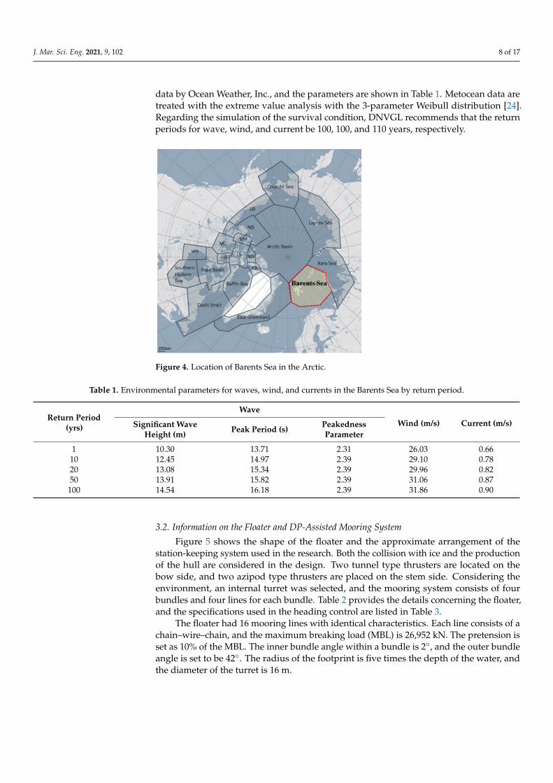
The Arctic floater in this research is targeted to be used in the Barents Sea, as shownin Figure 4 [23]. The site is selected based on the analysis of the prospects concerningfuture possible oil and gas development. Even though the average depth of the seawateris about 230 m, the depth is assumed to be 200 m, and it is assumed that the seafloor isflat. The environmental conditions are analyzed from the ocean wave 2012 (GROW2012)

J. Mar. Sci. Eng. 2021, 9, 102 8 of 17

data by Ocean Weather, Inc., and the parameters are shown in Table 1. Metocean data aretreated with the extreme value analysis with the 3-parameter Weibull distribution [24].Regarding the simulation of the survival condition, DNVGL recommends that the returnperiods for wave, wind, and current be 100, 100, and 110 years, respectively.

J. Mar. Sci. Eng. 2021, 9, x FOR PEER REVIEW 8 of 18

treated with the extreme value analysis with the 3-parameter Weibull distribution [24]. Regarding the simulation of the survival condition, DNVGL recommends that the return periods for wave, wind, and current be 100, 100, and 110 years, respectively.

Figure 4. Location of Barents Sea in the Arctic.

Table 1. Environmental parameters for waves, wind, and currents in the Barents Sea by return period.

Return Period (yrs) Wave

Wind (m/s) Current (m/s) Significant Wave Height (m) Peak Period (s) Peakedness Parameter

1 10.30 13.71 2.31 26.03 0.66 10 12.45 14.97 2.39 29.10 0.78 20 13.08 15.34 2.39 29.96 0.82 50 13.91 15.82 2.39 31.06 0.87 100 14.54 16.18 2.39 31.86 0.90

3.2. Information on the Floater and DP-Assisted Mooring System Figure 5 shows the shape of the floater and the approximate arrangement of the sta-

tion-keeping system used in the research. Both the collision with ice and the production of the hull are considered in the design. Two tunnel type thrusters are located on the bow side, and two azipod type thrusters are placed on the stem side. Considering the environ-ment, an internal turret was selected, and the mooring system consists of four bundles and four lines for each bundle. Table 2 provides the details concerning the floater, and the specifications used in the heading control are listed in Table 3.

(a) (b)

Figure 4. Location of Barents Sea in the Arctic.

Table 1. Environmental parameters for waves, wind, and currents in the Barents Sea by return period.

Return Period(yrs)

Wave

Wind (m/s) Current (m/s)Significant WaveHeight (m) Peak Period (s) Peakedness

Parameter

1 10.30 13.71 2.31 26.03 0.6610 12.45 14.97 2.39 29.10 0.7820 13.08 15.34 2.39 29.96 0.8250 13.91 15.82 2.39 31.06 0.87100 14.54 16.18 2.39 31.86 0.90

3.2. Information on the Floater and DP-Assisted Mooring System

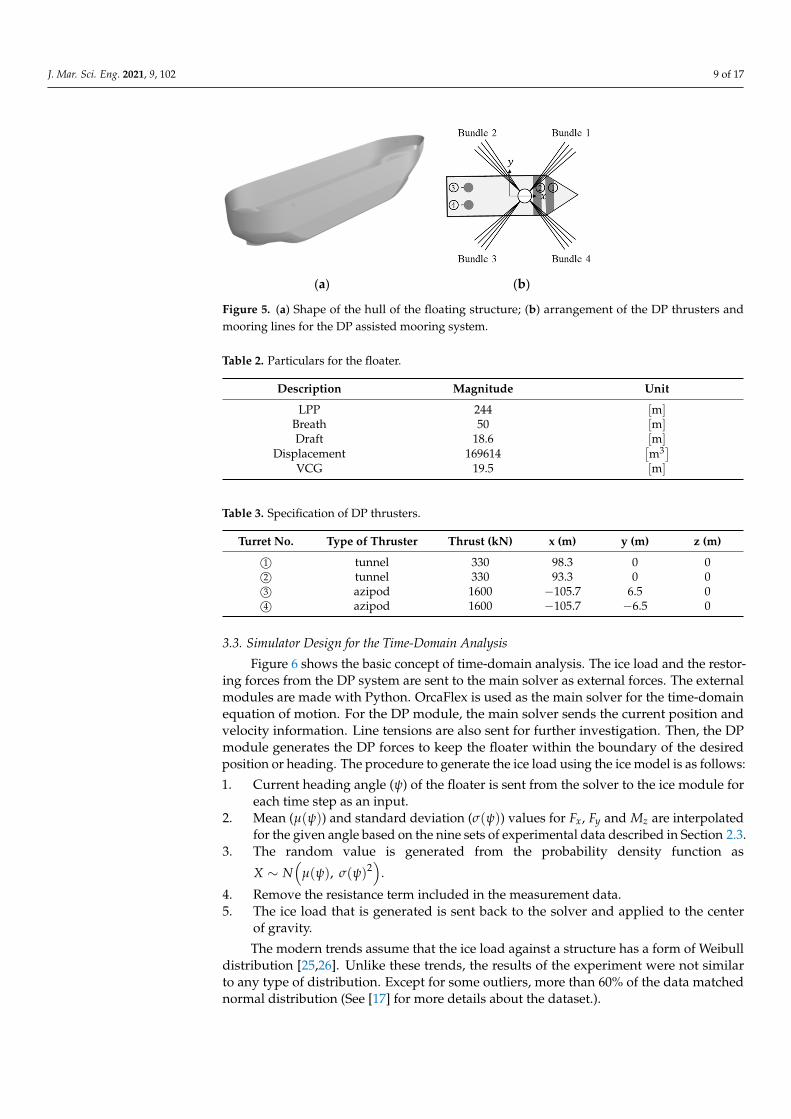
Figure 5 shows the shape of the floater and the approximate arrangement of thestation-keeping system used in the research. Both the collision with ice and the productionof the hull are considered in the design. Two tunnel type thrusters are located on thebow side, and two azipod type thrusters are placed on the stem side. Considering theenvironment, an internal turret was selected, and the mooring system consists of fourbundles and four lines for each bundle. Table 2 provides the details concerning the floater,and the specifications used in the heading control are listed in Table 3.

The floater had 16 mooring lines with identical characteristics. Each line consists of achain–wire–chain, and the maximum breaking load (MBL) is 26,952 kN. The pretension isset as 10% of the MBL. The inner bundle angle within a bundle is 2◦, and the outer bundleangle is set to be 42◦. The radius of the footprint is five times the depth of the water, andthe diameter of the turret is 16 m.

J. Mar. Sci. Eng. 2021, 9, 102 9 of 17

J. Mar. Sci. Eng. 2021, 9, x FOR PEER REVIEW 8 of 18

treated with the extreme value analysis with the 3-parameter Weibull distribution [24]. Regarding the simulation of the survival condition, DNVGL recommends that the return periods for wave, wind, and current be 100, 100, and 110 years, respectively.

Figure 4. Location of Barents Sea in the Arctic.

Table 1. Environmental parameters for waves, wind, and currents in the Barents Sea by return period.

Return Period (yrs) Wave

Wind (m/s) Current (m/s) Significant Wave Height (m) Peak Period (s) Peakedness Parameter

1 10.30 13.71 2.31 26.03 0.66 10 12.45 14.97 2.39 29.10 0.78 20 13.08 15.34 2.39 29.96 0.82 50 13.91 15.82 2.39 31.06 0.87 100 14.54 16.18 2.39 31.86 0.90

3.2. Information on the Floater and DP-Assisted Mooring System Figure 5 shows the shape of the floater and the approximate arrangement of the sta-

tion-keeping system used in the research. Both the collision with ice and the production of the hull are considered in the design. Two tunnel type thrusters are located on the bow side, and two azipod type thrusters are placed on the stem side. Considering the environ-ment, an internal turret was selected, and the mooring system consists of four bundles and four lines for each bundle. Table 2 provides the details concerning the floater, and the specifications used in the heading control are listed in Table 3.

(a) (b)

Figure 5. (a) Shape of the hull of the floating structure; (b) arrangement of the DP thrusters andmooring lines for the DP assisted mooring system.

Table 2. Particulars for the floater.

Description Magnitude Unit

LPP 244 [m]Breath 50 [m]Draft 18.6 [m]

Displacement 169614[m3]

VCG 19.5 [m]

Table 3. Specification of DP thrusters.

Turret No. Type of Thruster Thrust (kN) x (m) y (m) z (m)

1© tunnel 330 98.3 0 02© tunnel 330 93.3 0 03© azipod 1600 −105.7 6.5 04© azipod 1600 −105.7 −6.5 0

3.3. Simulator Design for the Time-Domain Analysis

Figure 6 shows the basic concept of time-domain analysis. The ice load and the restor-ing forces from the DP system are sent to the main solver as external forces. The externalmodules are made with Python. OrcaFlex is used as the main solver for the time-domainequation of motion. For the DP module, the main solver sends the current position andvelocity information. Line tensions are also sent for further investigation. Then, the DPmodule generates the DP forces to keep the floater within the boundary of the desiredposition or heading. The procedure to generate the ice load using the ice model is as follows:

1. Current heading angle (ψ) of the floater is sent from the solver to the ice module foreach time step as an input.

2. Mean (µ(ψ)) and standard deviation (σ(ψ)) values for Fx, Fy and Mz are interpolatedfor the given angle based on the nine sets of experimental data described in Section 2.3.

3. The random value is generated from the probability density function as

X ∼ N(

µ(ψ), σ(ψ)2)

.

4. Remove the resistance term included in the measurement data.5. The ice load that is generated is sent back to the solver and applied to the center

of gravity.

The modern trends assume that the ice load against a structure has a form of Weibulldistribution [25,26]. Unlike these trends, the results of the experiment were not similarto any type of distribution. Except for some outliers, more than 60% of the data matchednormal distribution (See [17] for more details about the dataset.).

J. Mar. Sci. Eng. 2021, 9, 102 10 of 17

J. Mar. Sci. Eng. 2021, 9, x FOR PEER REVIEW 9 of 18

Figure 5. (a) Shape of the hull of the floating structure; (b) arrangement of the DP thrusters and mooring lines for the DP assisted mooring system.

Table 2. Particulars for the floater.

Description Magnitude Unit LPP 244 [m]

Breath 50 [m] Draft 18.6 [m]

Displacement 169614 [m ] VCG 19.5 [m]

Table 3. Specification of DP thrusters.

Turret No. Type of Thruster Thrust (kN) x (m) y (m) z (m) ① tunnel 330 98.3 0 0 ② tunnel 330 93.3 0 0 ③ azipod 1600 −105.7 6.5 0 ④ azipod 1600 −105.7 −6.5 0

The floater had 16 mooring lines with identical characteristics. Each line consists of a chain–wire–chain, and the maximum breaking load (MBL) is 26,952 kN. The pretension is set as 10% of the MBL. The inner bundle angle within a bundle is 2°, and the outer bundle angle is set to be 42°. The radius of the footprint is five times the depth of the water, and the diameter of the turret is 16 m.

3.3. Simulator Design for the Time-Domain Analysis Figure 6 shows the basic concept of time-domain analysis. The ice load and the restor-

ing forces from the DP system are sent to the main solver as external forces. The external modules are made with Python. OrcaFlex is used as the main solver for the time-domain equation of motion. For the DP module, the main solver sends the current position and ve-locity information. Line tensions are also sent for further investigation. Then, the DP module generates the DP forces to keep the floater within the boundary of the desired position or heading. The procedure to generate the ice load using the ice model is as follows: 1. Current heading angle (𝜓) of the floater is sent from the solver to the ice module for

each time step as an input. 2. Mean (𝜇(𝜓)) and standard deviation (𝜎(𝜓)) values for 𝐹 , 𝐹 and 𝑀 are interpo-

lated for the given angle based on the nine sets of experimental data described in Section 2.3.

3. The random value is generated from the probability density function as 𝑋 ∼𝑁(𝜇(𝜓), 𝜎(𝜓) ). 4. Remove the resistance term included in the measurement data. 5. The ice load that is generated is sent back to the solver and applied to the center of

gravity.

Figure 6. Dynamic motion analysis with ice and DP modules in the time domain with a motion solver. Figure 6. Dynamic motion analysis with ice and DP modules in the time domain with a motion solver.

3.4. Setup of the Environmental Conditions for the Time-Domain Analysis

The environmental conditions for the simulation are shown in Table 4 and Figure 7.Generally, the time-domain analysis for the station-keeping system is performed assumingthe survival condition, which has a 100-year return period for waves. However, in the Arcticregion, harsh waves do not coexist with highly concentrated ice. Therefore, the generalsurvival conditions for waves, winds, and currents with ice are conditions too severe forthe floater. This is because of the damping effect that the covered ice has on the wave [27].Not much research has been completed on how to apply the ice–wave interaction in themotion simulation. In this research, a 1-year return period of the ocean wave selected, and ithas the smallest value in Table 1 and is used in the simulation. The 10-year and 100-yearreturn periods are applied for the current and wind, respectively, as directed by DNVGL.The ice parameters are the same values used in the ice tank experiment. The ARC 7condition of the Russian Maritime Register of Shipping is considered in deciding theparameters.

Table 4. Simulated conditions of the waves, wind, current, and ice.

Wave Wind Current Ice

Hs(m)

Tp(s) Y Velocity

(m/s)Velocity

(m/s)Thickness

(m)Length

(m)Speed(m/s) Concentration Shape

10.30 13.71 2.31 31.86 0.78 1.4 12 0.514 0.8 irregular

J. Mar. Sci. Eng. 2021, 9, x FOR PEER REVIEW 10 of 18

The modern trends assume that the ice load against a structure has a form of Weibull distribution [25,26]. Unlike these trends, the results of the experiment were not similar to any type of distribution. Except for some outliers, more than 60% of the data matched normal distribution (See [17] for more details about the dataset.).

3.4. Setup of the Environmental Conditions for the Time-Domain Analysis The environmental conditions for the simulation are shown in Table 4 and Figure 7.

Generally, the time-domain analysis for the station-keeping system is performed assum-ing the survival condition, which has a 100-year return period for waves. However, in the Arctic region, harsh waves do not coexist with highly concentrated ice. Therefore, the gen-eral survival conditions for waves, winds, and currents with ice are conditions too severe for the floater. This is because of the damping effect that the covered ice has on the wave [27]. Not much research has been completed on how to apply the ice–wave interaction in the motion simulation. In this research, a 1-year return period of the ocean wave selected, and it has the smallest value in Table 1 and is used in the simulation. The 10-year and 100-year return periods are applied for the current and wind, respectively, as directed by DNVGL. The ice parameters are the same values used in the ice tank experiment. The ARC 7 condition of the Russian Maritime Register of Shipping is considered in deciding the parameters.

Table 4. Simulated conditions of the waves, wind, current, and ice.

Wave Wind Current Ice Hs (m)

Tp (s)

𝚼 Velocity (m/s)

Velocity (m/s)

Thickness (m)

Length (m)

Speed (m/s) Concentration Shape

10.30 13.71 2.31 31.86 0.78 1.4 12 0.514 0.8 irregular

Figure 7. Directions of the complex environmental loads.

The directions of the loads are set according to the DNVGL standard for the non-collinear condition. Waves are from the head sea, and the wind and current are applied to the floater at 30° and 45° angles with respect to the wave. The direction of the ice is not well defined for the time-domain simulation. As mentioned earlier, it is assumed that the ice drifts between the current and wind directions.

4. Simulation Results Simulation is conducted for the floater using the system described in Section 3.3 based

on the environmental conditions in Section 3.4. The heading control mode is selected for the DP system in order to reflect the difficulties associated with the on-site operation of the DP vessel in the ice-covered sea. The target heading is set to be against the direction of the ice drift. According to the DNVGL standard, 20 seeds are selected randomly for the irregular waves, and a 3-h time-domain simulation is conducted for each seed.

Figure 8 is an example to show the effect of ice loads on the station-keeping perfor-mance. Simulation results were compared for a total of four cases, with and without ice and DP for the same environmental conditions. As mentioned earlier, the MPM value is

Figure 7. Directions of the complex environmental loads.

The directions of the loads are set according to the DNVGL standard for the non-collinear condition. Waves are from the head sea, and the wind and current are applied tothe floater at 30◦ and 45◦ angles with respect to the wave. The direction of the ice is notwell defined for the time-domain simulation. As mentioned earlier, it is assumed that theice drifts between the current and wind directions.

4. Simulation Results

Simulation is conducted for the floater using the system described in Section 3.3 basedon the environmental conditions in Section 3.4. The heading control mode is selected forthe DP system in order to reflect the difficulties associated with the on-site operation ofthe DP vessel in the ice-covered sea. The target heading is set to be against the direction ofthe ice drift. According to the DNVGL standard, 20 seeds are selected randomly for theirregular waves, and a 3-h time-domain simulation is conducted for each seed.

J. Mar. Sci. Eng. 2021, 9, 102 11 of 17

Figure 8 is an example to show the effect of ice loads on the station-keeping perfor-mance. Simulation results were compared for a total of four cases, with and without iceand DP for the same environmental conditions. As mentioned earlier, the MPM value isthe point at which the cumulative value is 37% of the Gumbel probability density func-tion. Therefore, the smaller circles indicate that the floater stays mostly within a smallerboundary. The maximum offset under no ice condition is 9.9 m, whereas the one underice condition is 16.8 m. With the ice, the MPM value is 10.1 m without ice and 15.1 m withice. The result indicates the significance of ice-induced forces on the station-keeping of thegiven floating structure in an ice-covered sea.

J. Mar. Sci. Eng. 2021, 9, x FOR PEER REVIEW 11 of 18

the point at which the cumulative value is 37% of the Gumbel probability density function. Therefore, the smaller circles indicate that the floater stays mostly within a smaller bound-ary. The maximum offset under no ice condition is 9.9 m, whereas the one under ice con-dition is 16.8 m. With the ice, the MPM value is 10.1m without ice and 15.1 m with ice. The result indicates the significance of ice-induced forces on the station-keeping of the given floating structure in an ice-covered sea.

Figure 9 shows the trajectories of the floater in 3-h simulations for both the DPAM and mooring only scenarios. Since the same seed gives the same phases and consequently the same train of waves, two simulations are run for a single seed, i.e., one for DPAM and another for the mooring-only scenario. This was repeated 20 times with 20 different seeds. Since the actual number of seeds was selected randomly in this research, the results were organized as case 1 to case 20 for easy identification.

The allowable offset was set as 20 m, which was 10% of the depth of the water. For the mooring-only system, in some cases, the position approached the limit boundary (i.e., case 18, case 20, and others). With the heading control by DPAM, the trajectory of the floater remained stably within the allowable offset.

Figure 8. The comparison of station-keeping performance to analyze the effects of ice loads. Figure 8. The comparison of station-keeping performance to analyze the effects of ice loads.

Figure 9 shows the trajectories of the floater in 3-h simulations for both the DPAMand mooring only scenarios. Since the same seed gives the same phases and consequentlythe same train of waves, two simulations are run for a single seed, i.e., one for DPAM andanother for the mooring-only scenario. This was repeated 20 times with 20 different seeds.Since the actual number of seeds was selected randomly in this research, the results wereorganized as case 1 to case 20 for easy identification.

The allowable offset was set as 20 m, which was 10% of the depth of the water. For themooring-only system, in some cases, the position approached the limit boundary (i.e., case18, case 20, and others). With the heading control by DPAM, the trajectory of the floaterremained stably within the allowable offset.

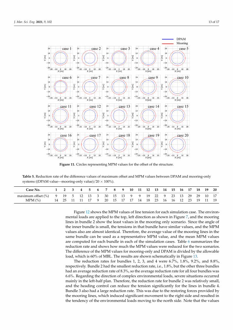
Figure 10 shows circles by setting the radius to be the maximum offset during the 3-hsimulation. This enables the identification and comparison of the performances of the twoscenarios. The circles in Figure 11 are the MPM values after the statistical process for theperformance evaluation for three hours.

In some cases, the difference in the maximum offset is small (case 3, case 6). This is be-cause the environment is relatively mild, and the mooring-only system works fine. In somecases, i.e., when the offset is large due to the severe environmental loads, the difference isrelatively small. This is due to a freak wave, which is a much larger wave than the height ofa significant wave. With such a rogue wave, the DP system cannot work effectively againstthe environment.

Table 5 shows the improvement in the performance of DPAM over the mooring-onlysystem. The numbers show the rate of improvement with respect to the allowable offset of20 m. The mean value in terms of the maximum offset is 15.4% (3.1 m).

J. Mar. Sci. Eng. 2021, 9, 102 12 of 17J. Mar. Sci. Eng. 2021, 9, x FOR PEER REVIEW 12 of 18

Figure 9. Trajectories of the floater for a 3-h simulation. Dynamic positioning assisted mooring (DPAM) and mooring only systems were compared with the same seed. Simulations were repeated for 20 different seeds.

Figure 10 shows circles by setting the radius to be the maximum offset during the 3-h simulation. This enables the identification and comparison of the performances of the two scenarios. The circles in Figure 11 are the MPM values after the statistical process for the performance evaluation for three hours.

In some cases, the difference in the maximum offset is small (case 3, case 6). This is because the environment is relatively mild, and the mooring-only system works fine. In some cases, i.e., when the offset is large due to the severe environmental loads, the differ-ence is relatively small. This is due to a freak wave, which is a much larger wave than the height of a significant wave. With such a rogue wave, the DP system cannot work effec-tively against the environment.

Figure 9. Trajectories of the floater for a 3-h simulation. Dynamic positioning assisted mooring (DPAM) and mooring onlysystems were compared with the same seed. Simulations were repeated for 20 different seeds.

J. Mar. Sci. Eng. 2021, 9, x FOR PEER REVIEW 13 of 18

Figure 10. Circles with radii representing the maximum offset for each simulation.

Figure 11. Circles representing MPM values for the offset of the structure.

Figure 10. Circles with radii representing the maximum offset for each simulation.

J. Mar. Sci. Eng. 2021, 9, 102 13 of 17

J. Mar. Sci. Eng. 2021, 9, x FOR PEER REVIEW 13 of 18

Figure 10. Circles with radii representing the maximum offset for each simulation.

Figure 11. Circles representing MPM values for the offset of the structure. Figure 11. Circles representing MPM values for the offset of the structure.

Table 5. Reduction rate of the difference values of maximum offset and MPM values between DPAM and mooring-onlysystems ((DPAM value—mooring-only value)/20 × 100%).

Case No. 1 2 3 4 5 6 7 8 9 10 11 12 13 14 15 16 17 18 19 20

maximum offset (%) 9 19 5 12 13 3 30 15 13 9 9 19 22 9 23 13 29 29 10 17MPM (%) 14 25 11 11 17 9 20 15 17 17 14 18 23 16 16 12 23 19 11 19

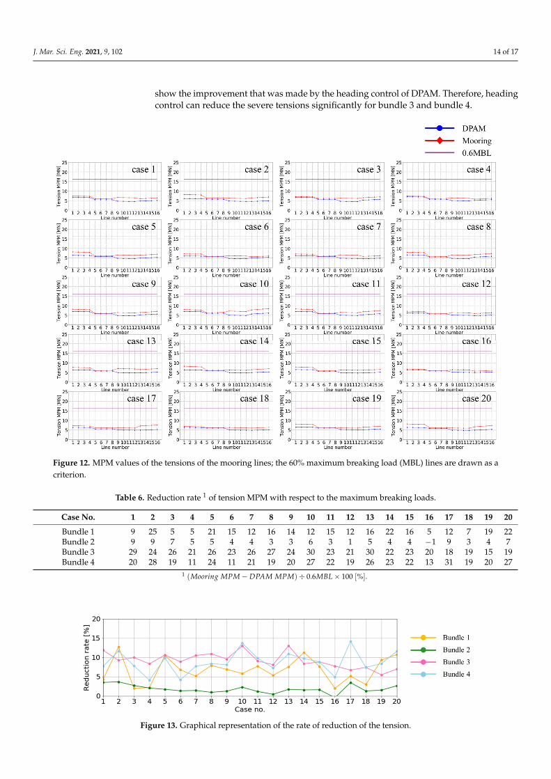
Figure 12 shows the MPM values of line tension for each simulation case. The environ-mental loads are applied to the top, left direction as shown in Figure 7, and the mooringlines in bundle 2 show the least values in the mooring only scenario. Since the angle ofthe inner bundle is small, the tensions in that bundle have similar values, and the MPMvalues also are almost identical. Therefore, the average value of the mooring lines in thesame bundle can be used as a representative MPM value, and the mean MPM valuesare computed for each bundle in each of the simulation cases. Table 6 summarizes thereduction rate and shows how much the MPM values were reduced for the two scenarios.The difference of the MPM values for mooring-only and DPAM is divided by the allowableload, which is 60% of MBL. The results are shown schematically in Figure 13.

The reduction rates for bundles 1, 2, 3, and 4 were 6.7%, 1.8%, 9.2%, and 8.8%,respectively. Bundle 2 had the smallest reduction rate, i.e., 1.8%, but the other three bundleshad an average reduction rate of 8.3%, so the average reduction rate for all four bundles was6.6%. Regarding the direction of complex environmental loads, severe situations occurredmainly in the left-half plan. Therefore, the reduction rate for bundle 2 was relatively small,and the heading control can reduce the tension significantly for the lines in bundle 4.Bundle 3 also had a large reduction rate. This was due to the restoring forces provided bythe mooring lines, which induced significant movement to the right side and resulted inthe tendency of the environmental loads moving to the north side. Note that the values

J. Mar. Sci. Eng. 2021, 9, 102 14 of 17

show the improvement that was made by the heading control of DPAM. Therefore, headingcontrol can reduce the severe tensions significantly for bundle 3 and bundle 4.

J. Mar. Sci. Eng. 2021, 9, x FOR PEER REVIEW 14 of 18

Table 5 shows the improvement in the performance of DPAM over the mooring-only system. The numbers show the rate of improvement with respect to the allowable offset of 20 m. The mean value in terms of the maximum offset is 15.4% (3.1 m).

Table 5. Reduction rate of the difference values of maximum offset and MPM values between DPAM and mooring-only systems ((DPAM value—mooring-only value)/20 × 100%).

Case No. 1 2 3 4 5 6 7 8 9 10 11 12 13 14 15 16 17 18 19 20 maximum offset (%) 9 19 5 12 13 3 30 15 13 9 9 19 22 9 23 13 29 29 10 17

MPM (%) 14 25 11 11 17 9 20 15 17 17 14 18 23 16 16 12 23 19 11 19

Figure 12 shows the MPM values of line tension for each simulation case. The envi-ronmental loads are applied to the top, left direction as shown in Figure 7, and the moor-ing lines in bundle 2 show the least values in the mooring only scenario. Since the angle of the inner bundle is small, the tensions in that bundle have similar values, and the MPM values also are almost identical. Therefore, the average value of the mooring lines in the same bundle can be used as a representative MPM value, and the mean MPM values are computed for each bundle in each of the simulation cases. Table 6 summarizes the reduc-tion rate and shows how much the MPM values were reduced for the two scenarios. The difference of the MPM values for mooring-only and DPAM is divided by the allowable load, which is 60% of MBL. The results are shown schematically in Figure 13.

Figure 12. MPM values of the tensions of the mooring lines; the 60% maximum breaking load (MBL) lines are drawn as a criterion.

Figure 12. MPM values of the tensions of the mooring lines; the 60% maximum breaking load (MBL) lines are drawn as acriterion.

Table 6. Reduction rate 1 of tension MPM with respect to the maximum breaking loads.

Case No. 1 2 3 4 5 6 7 8 9 10 11 12 13 14 15 16 17 18 19 20

Bundle 1 9 25 5 5 21 15 12 16 14 12 15 12 16 22 16 5 12 7 19 22Bundle 2 9 9 7 5 5 4 4 3 3 6 3 1 5 4 4 −1 9 3 4 7Bundle 3 29 24 26 21 26 23 26 27 24 30 23 21 30 22 23 20 18 19 15 19Bundle 4 20 28 19 11 24 11 21 19 20 27 22 19 26 23 22 13 31 19 20 27

1 (Mooring MPM− DPAM MPM)÷ 0.6MBL× 100 [%].

J. Mar. Sci. Eng. 2021, 9, x FOR PEER REVIEW 15 of 18

Table 6. Reduction rate 1 of tension MPM with respect to the maximum breaking loads.

Case No. 1 2 3 4 5 6 7 8 9 10 11 12 13 14 15 16 17 18 19 20 Bundle 1 9 25 5 5 21 15 12 16 14 12 15 12 16 22 16 5 12 7 19 22 Bundle 2 9 9 7 5 5 4 4 3 3 6 3 1 5 4 4 −1 9 3 4 7 Bundle 3 29 24 26 21 26 23 26 27 24 30 23 21 30 22 23 20 18 19 15 19 Bundle 4 20 28 19 11 24 11 21 19 20 27 22 19 26 23 22 13 31 19 20 27

1 (𝑀𝑜𝑜𝑟𝑖𝑛𝑔 𝑀𝑃𝑀 − 𝐷𝑃𝐴𝑀 𝑀𝑃𝑀) 0.6𝑀𝐵𝐿 × 100 [%].

Figure 13. Graphical representation of the rate of reduction of the tension.

The reduction rates for bundles 1, 2, 3, and 4 were 6.7%, 1.8%, 9.2%, and 8.8%, respec-tively. Bundle 2 had the smallest reduction rate, i.e., 1.8%, but the other three bundles had an average reduction rate of 8.3%, so the average reduction rate for all four bundles was 6.6%. Regarding the direction of complex environmental loads, severe situations occurred mainly in the left-half plan. Therefore, the reduction rate for bundle 2 was relatively small, and the heading control can reduce the tension significantly for the lines in bundle 4. Bun-dle 3 also had a large reduction rate. This was due to the restoring forces provided by the mooring lines, which induced significant movement to the right side and resulted in the tendency of the environmental loads moving to the north side. Note that the values show the improvement that was made by the heading control of DPAM. Therefore, heading control can reduce the severe tensions significantly for bundle 3 and bundle 4.

Figure 14 shows the variation of the heading angles for each case. The target heading was set at −35°, which is the opposite direction from the drifting ice. The simulation results show that the heading control worked well and maintained the desired heading angle for the DPAM while showing a large fluctuation of the heading angle in the case of the sce-nario of mooring-only. Therefore, heading control can contribute both to tension control and position control by reducing the fluctuation of the heading angle, thereby resulting in a small drift against complex environmental loads, including ice-induced forces.

Figure 13. Graphical representation of the rate of reduction of the tension.

J. Mar. Sci. Eng. 2021, 9, 102 15 of 17

Figure 14 shows the variation of the heading angles for each case. The target headingwas set at−35◦, which is the opposite direction from the drifting ice. The simulation resultsshow that the heading control worked well and maintained the desired heading anglefor the DPAM while showing a large fluctuation of the heading angle in the case of thescenario of mooring-only. Therefore, heading control can contribute both to tension controland position control by reducing the fluctuation of the heading angle, thereby resulting ina small drift against complex environmental loads, including ice-induced forces.

J. Mar. Sci. Eng. 2021, 9, x FOR PEER REVIEW 16 of 18

Figure 14. Time history of the heading angles for a 3-h simulation.

5. Conclusions and Future Work The effect of the heading control by the DP system was investigated for an Arctic

floating structure. Based on the experimental data acquired using the ice tank at KRISO, an ice load was generated using a statistical process. Then, the ice force that was generated and applied to the specially designed structure, along with waves, winds, and currents, as components of complex environmental loads. The motion of the floater was analyzed for the conditions at the target site. Two scenarios were tested, i.e., the DPAM and the mooring-only system, and the results were compared. The heading control mode was set for DPAM, and 3-h time-domain simulations were conducted. The MPM values of the position offset and the line tension for both scenarios were derived from the results and compared to verify the effectiveness of the heading control. The main observations are summarized below: • The functionalities of the ice load generation module and the DP force generation

module were verified and applied to the time-domain analysis with a motion solver. These modules can be used to further assess various scenarios in harsh environmen-tal conditions.

• With the DPAM heading control, the maximum position offset was reduced to 3.1 m (15.4% of the allowable maximum offset of 20 m) based on the average of the 20 cases. The mean value for the reduction of MPM was about 3.3 m (16.3%). The target head-ing angle was set in the ice drift direction, which was between the wind and current directions. Therefore, the station-keeping performance was enhanced by reducing the drift of complex environmental loads.

• Except for bundle 2, which had the smallest tensions due to its configuration, the MPM values were reduced by 8.2% with respect to the 0.6 MBL, which was the design criterion Heading control reduces the beam sea situation and lowers the tension on the mooring lines due to the smaller floater motion.

Figure 14. Time history of the heading angles for a 3-h simulation.

5. Conclusions and Future Work

The effect of the heading control by the DP system was investigated for an Arcticfloating structure. Based on the experimental data acquired using the ice tank at KRISO,an ice load was generated using a statistical process. Then, the ice force that was generatedand applied to the specially designed structure, along with waves, winds, and currents,as components of complex environmental loads. The motion of the floater was analyzedfor the conditions at the target site. Two scenarios were tested, i.e., the DPAM and themooring-only system, and the results were compared. The heading control mode was setfor DPAM, and 3-h time-domain simulations were conducted. The MPM values of theposition offset and the line tension for both scenarios were derived from the results andcompared to verify the effectiveness of the heading control. The main observations aresummarized below:

• The functionalities of the ice load generation module and the DP force generationmodule were verified and applied to the time-domain analysis with a motion solver.These modules can be used to further assess various scenarios in harsh environmentalconditions.

• With the DPAM heading control, the maximum position offset was reduced to 3.1 m(15.4% of the allowable maximum offset of 20 m) based on the average of the 20 cases.The mean value for the reduction of MPM was about 3.3 m (16.3%). The target heading

J. Mar. Sci. Eng. 2021, 9, 102 16 of 17

angle was set in the ice drift direction, which was between the wind and currentdirections. Therefore, the station-keeping performance was enhanced by reducing thedrift of complex environmental loads.

• Except for bundle 2, which had the smallest tensions due to its configuration, theMPM values were reduced by 8.2% with respect to the 0.6 MBL, which was the designcriterion Heading control reduces the beam sea situation and lowers the tension onthe mooring lines due to the smaller floater motion.

The results of this research are expected to be used in redesigning the mooring lineswhen the Arctic floater is equipped with a DP system. The following items will be investi-gated further:

• It is necessary to consider the coupled effect between an ice load and other environ-mental loads. When the heading angle is larger than a certain limit, the DP thrusterscannot generate an adequate restoring force. This effect cannot be considered by thecurrent module used to generate the ice load. Therefore, a more precise ice modulewill be developed.

• The direction of the heading control is set such that it is the opposite of the driftdirection of the ice floe. This is to consider the significance of the ice load, but thedirection may not be the dominant direction in which the floater must be controlled.PID control may have limitations on this issue, and more-complicated, active-typecontrollers will be studied.

• Further investigation is necessary to determine the relationship between the conditionof the ice and a wave. This study considered a 1-year return period (for a significantwave height of 10.3 m), but the condition is still too harsh for the ice field with 80%concentration. Feasible environmental conditions will be analyzed for realistic motionanalysis in the time domain.

• As data related to structural design have yet to be prepared, no analysis of vibrationwas conducted. Further research is necessary because vibration studies related tonatural frequencies are essential for the designed floater.

Author Contributions: Conceptualization, H.H.K. and J.L.; methodology, S.J.L.; validation, D.-S.L.,J.-S.L. and S.J.L.; formal analysis, J.L. and K.H.J.; data curation, J.J.; writing—original draft prepara-tion, H.H.K.; writing—review and editing, J.L. All authors have read and agreed to the publishedversion of the manuscript.

Funding: This research was funded by the Ministry of Trade, Industry & Energy (MOTIE, Korea)under Industrial Technology Innovation Program No. 10063405 and No. 10070163.

Institutional Review Board Statement: Not applicable.

Informed Consent Statement: Not applicable.

Data Availability Statement: Restrictions apply to the availability of these data. Data was obtainedfrom KRISO and are available with the permission of KRISO.

Conflicts of Interest: The authors declare no conflict of interest.

References1. Zhou, L.; Moan, T.; Riska, K. Heading control for turret-moored vessel in level ice based on Kalman filter with thrust allocation.

J. Mar. Sci. Tech. 2013, 18, 460–470. [CrossRef]2. Ansari, K.A. Effect of vessel hydrodynamic mass on the station-keeping response of a moored offshore vessel. Trans. ASME 1989,

108, 52–58. [CrossRef]3. Choung, J.; Jeon, G.-Y.; Kim, Y. Study on Effective Arrangement of Mooring Lines of Floating-Type Combined Renewable Energy

Platform. J. Ocean Eng. Tech. 2013, 27, 22–32. [CrossRef]4. API, D. Analysis of Stationkeeping Systems for Floating Structures; API-RP-2SK.; American Petroleum Institute: Washington, DC,

USA, 2005.5. Moran, K.; Backman, J.; Farrell, J.W. Deepwater drilling in the Arctic Ocean’s permanent sea ice. Proc. Int. Ocean Drill. Program

2006, 302, 2.

J. Mar. Sci. Eng. 2021, 9, 102 17 of 17

6. Liferov, P.; Serre, N.; Kerkeni, S.; Bridges, R.; Guo, F. Station-Keeping Trials in Ice: Test Scenarios. In Proceedings of the ASME2018 37th International Conference on Ocean, Offshore and Arctic Engineering, Madrid, Spain, 17–22 June 2018; American Societyof Mechanical Engineers: New York, NY, USA, 2018.

7. Kerkeni, S.; Liferov, P.; Serre, N.; Bridges, R.; Jorgensen, F. Station-Keeping Trials in Ice: Dynamic Positioning in Ice-Results andLearnings. In Proceedings of the ASME 2018 37th International Conference on Ocean, Offshore and Arctic Engineering, Madrid,Spain, 17–22 June 2018; American Society of Mechanical Engineers: New York, NY, USA, 2018.

8. Jenssen, N.A.; Hals, T.; Jochmann, P.; Haase, A.; dal Santo, X.; Kerkeni, S.; Doucy, O.; Gürtner, A.; Støle Hetschel, S.;Moslet, P.O.; et al. DYPIC—A Multi-National R&D Project on DP Technology in Ice. In Proceedings of the Dynamic Posi-tioning Conference, Houston, TX, USA, 9 October 2012.

9. Kerkeni, S.; Santo, X.D.; Doucy, O.; Jochmann, P.; Haase, A.; Metrikin, I.; Løset, S.; Jenssen, N.A.; Hals, T.; Gürtner, A.; et al.DYPIC project: Technological and scientific progress opening new perspectives. In Proceedings of the OTC Arctic TechnologyConference, Houston, TX, USA, 13 February 2014.

10. Wang, J.; Sayeed, T.; Millan, D.; Gash, R.; Islam, M.; Millan, J. Ice Model Tests for Dynamic Positioning Vessel in Managed Ice.In Proceedings of the Arctic Technology Conference, St. John’s, NL, Canada, 24–26 October 2016.

11. Lubbad, R.; Løset, S.; Lu, W.; Tsarau, A.; van den Berg, M. An overview of the Oden Arctic Technology Research Cruise 2015(OATRC2015) and numerical simulations performed with SAMS driven by data collected during the cruise. Cold Reg. Sci. Technol.2018, 156, 1–22. [CrossRef]

12. Lubbad, R.; Løset, S.; Lu, W.; Tsarau, A.; Van Den Berg, M. Simulator for arctic marine structures (SAMS). In Proceedings of theASME 2018 37th International Conference on Offshore Mechanics and Arctic Engineering—OMAE, Madrid, Spain, 17 June 2018.

13. Raza, N.; van der Berg, M.; Lu, W.; Lubbad, R. Analysis of Oden Icebreaker Performance in Level Ice using Simulator for ArcticMarine Structures (SAMS). In Proceedings of the 25th International Conference on Port and Ocean Engineering under ArcticConditions, Delft, The Netherlands, 9–13 June 2019.

14. Daley, C.; Alawneh, S.; Peters, D.; Quinton, B.; Colbourne, B. GPU Modeling of Ship Operations in Pack Ice. In Proceedings of theInternational Conference and Exhibition on Performance of Ships and Structures in Ice, Banff, AB, Canada, 17–20 September 2012.

15. Daley, C.G.; Alawneh, S.; Peters, D.; Blades, G.; Colbourne, B. Simulation of Managed Sea Ice Loads on a Floating OffshorePlatform using GPU-Event Mechanics. In Proceedings of the International Conference and Exhibition on Performance of Shipsand Structures in Ice IceTech, Banff, AB, Canada, 28–31 July 2014.

16. Kim, Y.-S.; Kim, J.-H.; Kang, K.-J.; Han, S.; Kim, J. Ice Load Generation in Time Domain Based on Ice Load Spectrum for ArcticOffshore Structures. J. Ocean Eng. Tech. 2018, 32, 411–418. [CrossRef]

17. Kang, H.H.; Lee, D.; Lim, J.; Lee, S.J.; Jang, J.; Jung, K.; Lee, J. Development of Ice Load Generation Module to Evaluate StationKeeping Performance for Arctic Floating Structures in Time Domain. J. Ocean Eng. Tech. 2020, 34, 394–405. [CrossRef]

18. Ghafari, H.; Dardel, M. Parametric study of catenary mooring system on the dynamic response of the semi-submersible platform.Ocean Eng. 2018, 153, 319–332. [CrossRef]

19. Orcaflex Morison Elements. Available online: https://www.orcina.com/webhelp/OrcaFlex/Content/html/Morisonelements.htm (accessed on 20 December 2020).

20. Trunbull, I.D.; Torbati, R.Z.; Taylor, R.S. Relative influences of the metocean forcings on the drifting ice pack and estimation ofinternal ice stress gradients in the Labrador Sea. J. Geophys. Res. Oceans 2017, 122, 5970–5997. [CrossRef]

21. DNV, G.L. Offshore Standard: Position Mooring; DNVGL-OS-E301; DNV GL: Oslo, Norway, 2015.22. Veritas, B. Classification of Mooring Systems for Permanent and Mobile Offshore Units; NR-493-DT-R03-E; BV: Neuilly sur Seine,

France, 2015.23. IUCN/SSC PBSH Barents Sea (BS). Available online: http://pbsg.npolar.no/en/status/populations/barents-sea.html (accessed

on 20 December 2020).24. Park, S.B.; Shin, S.Y.; Shin, D.G.; Jung, K.H.; Choi, Y.H.; Lee, J.; Lee, S.J. Extreme Value Analysis of Metocean Data for Barents Sea.

J. Ocean Eng. Technol. 2020, 34, 26–36. [CrossRef]25. Kujala, P.; Suominen, M.; Riska, K. Statistics of Ice Loads Measured on Mt Uikku in the Baltic. In Proceedings of the 20th

International Conference on Port and Ocean Engineering under Arctic Conditions, Luleå, Sweden, 9–12 June 2009.26. Suominen, M.; Kujala, P.; Romanoff, J.; Remes, H. Influence of load length on short-term ice load statistics in full-scale. Mar. Struct.

2017, 52, 153–172. [CrossRef]27. Sutherland, B.R.; Balmforth, N.J. Damping of surface waves by floating particles. Phys. Rev. Fluids 2019, 4, 010804. [CrossRef]