A Study on the Dynamic Relationship Between Financial ...

Journal of Economics and Sustainable Development www.iiste.org

ISSN 2222-1700 (Paper) ISSN 2222-2855 (Online)

Vol.10, No.14, 2020

77

A Study on the Dynamic Relationship Between Financial

Development and Investment: Evidence from Sub-Saharan Africa

*Isaac Okyere Paintsil Zhao Xicang

Jiangsu University, School of Finance and Economics, 301 Xuefu Road, Zhenjiang. China PRC.

Abstract

The relationship between financial development and investment has become the central focus for empirical studies

since the emergence of endogenous growth models. Bank-based measures and Financial markets-based measures

have often been used as proxies for financial development in many studies. However, results based on these proxies

have often yielded different interpretations since the concept of financial development is broad and a

multidimensional process. The Financial development index of the International Monetary Fund (IMF) presents a

more comprehensive measure for financial development, and it is also useful for investigating financial

development and other economic outcomes. Also, investment is a versatile concept since it takes on many forms

and sources. We adopt the panel VAR estimation techniques to examine the endogenous relationship between

financial development and investment using the Financial development index, general government investment,

private investment, and foreign direct investment (FDI) as dependent variables. The study reveals that private

investment has a positive endogenous relationship with financial development. Moreover, the causal relationship

between financial development and private investment is bilateral. Also, financial development has a positive

influence on FDI. Furthermore, the study suggests that financial development has a strongly exogenous

relationship with General government investment.

Keywords: Financial development index; Private investment; General government investment; Foreign direct

investment; Panel VAR.

DOI: 10.7176/JESD/10-14-09

Publication date:July 31st 2020

1. Introduction.

The impact of financial development on economic growth is well entrenched in economic literature (see Goldsmith,

(1969); Beck et al., (2000); Demetriades and Hussein, (1996); King (1993); Levine (1997); Levine and Zervos

(1998); Demirgüç-Kunt and Levine (2004); Rousseau and Wachtel (2011)). Proponents of Endogenous growth

also emphasize the importance of investment in the finance-growth nexus (Levine, 1997). Levine and Renelt (1992)

suggest that an increase in the volume of investment in an economy intensifies the rate of economic growth. Thus,

from the endogenous growth point of view, financial development leads to increased savings, which raises the

level of capital accumulation for investment, and also leads to productivity (Demetriades and Hussein (1996);

Levine (1997)).

A typical situation which mirrors the endogenous growth explanation is the recent gains in the economic

growth of some sub-Saharan African countries where in the past financial development was lagging as a result of

macroeconomic and political instability which plunged many countries the subregion into economic woes and

widespread poverty. Some countries in the sub-Saharan Africa region underwent various forms of fiscal and

financial reforms which aimed at boosting the investment. In recent year concrete evidence with respect to GDP

seems to suggest that those policy interventions made an impact. According to an IMF report, the sub-Saharan

African region is now becoming the fastest growing after Asia (IMF, 2016).

Empirical studies on financial development and investment are a central focus for many researchers and

endogenous growth proponents. Majority of these studies makes use of bank-based variables or financial market-

based variables or both in many instances as proxies for financial development. However, the results have often

yielded different interpretations due to the broad and multidimensional nature of financial development. Sackyi et

al., (2016) underscore this opinion and echo that the impact of financial development on investment is susceptible

to the indicators used for financial development since the notion of financial development is broad, and

multidimensional.

Sahay et al. (2015) and Svirydzenka (2016) develop the Financial Development index that summarize how

developed financial institutions and financial markets are according to their depth, access, and efficiency.

According to Svirydzenka (2016), the Financial Development index presents a more comprehensive measure of

financial development, and it is also useful for investigating financial development and other economic outcomes.

However, no attempt has yet been made to use the Financial Development index to explore the dynamic

relationship between financial development and investment in sub-Saharan Africa. This paper attempts to fill this

gap.

This study adopts a country level panel data and the panel VAR method of estimation that based on the

generalized method of moments (GMM) to empirically identify some main issues on financial development and



Vol.10, No.14, 2020

78

investment in sub-Saharan Africa and make some recommendations. The application of panel VAR analysis by

the GMM allows us to check for endogenous interactions between financial development and investment. The

GMM also allows us to take care of small samples, endogeneity problems, and omitted variables. In addition to

the stated objective, this study contributes to the growing literature on financial development and investment in

two ways. The contribution of this study is two-fold:

1. We focus on sub-Saharan Africa, where major financial innovation and FinTech business activities

are taking place. Thus, this study echoes the “finance-investment” interaction in sub-Saharan African

countries and also provides a sub-Saharan African perspective on the subject.

2. Also, investment itself is a versatile concept, in that, it takes on different forms and sources;

consequently, we adopt three different forms of investment, namely; Private investment, General

government investment, and Foreign direct investment (FDI) for the analysis.

The rest of the paper is organized as follows. A brief review of some empirical literature is provided. Next,

the data used in the study, followed by an outline of the methodology and model in the empirical study, are

presented. Then the findings and discussions are provided. The last section provides the conclusion for the study.

2. Brief literature review

We discuss empirical literature on financial development and investment in subsection 2.1 and also review relevant

empirical studies on financial development and FDI in subsection 2.2.

2.1. Financial development and investment

Caporale et al., (2005) study the relationship between financial development and investment using financial market

variables on Chile, Korea, Malaysia, and the Philippines for the period 1979 to 1998. They conduct the Toda and

Yamamoto causality test to determine the direction of causality within the variables. Their conclusion suggests

that stock market development Granger‐causes investment productivity in all four countries. Similarly, Carp (2012)

use data on Romania for the period 1995 to 2010. He adopts vector autoregressive models (VAR) and Granger

causality approach to observe the causal direction between financial development and investment. The variables

used in the study include; the annual percentage growth of GDP at market prices, local currency market

capitalization, turnover ratio, stocks traded, and total investment as a percentage of GDP. The outcome indicates

that stock market capitalization Granger-causes investment.

Rousseau and Vuthipadadorn (2005) conduct a study on financial development and investment in ten Asian

countries for the period 1950 to 2000. They adopt vector autoregressive models (VAR) and vector error correction

(VECM) econometric techniques for the analysis. They use bank development variables as proxy for financial

development. The study reveals that financial development leads to investment growth in seven countries, namely;

India, Japan, Korea, Malaysia, Pakistan, Sri Lanka, and Thailand. Further, their findings show a bi-directional

relationship between Financial Development and Investment for the Philippines and Singapore but no causal

relationship between the variables for Indonesia. Hamdi et al. (2013) also study the nexus between Financial

development and investment in Tunisia by conducting Multivariate Granger causality and vector error correction

model (VECM). Their findings show that financial development Granger-cause Investment. Likewise, Asongu

(2014) study the finance and investment dynamics of sixteen African countries using the vector error correction

model (VECM) and several banking development indicators in his study. The finding shows that financial

development Granger-cause investment.

Chaudhry et al. (2012), use the Engle-Granger and ECM approach to assesses the effectiveness of financial

development in promoting investment in Pakistan over the period 1972–2006. The study attempts to capture the

multidimensional aspects of financial development by including both banking development measures and financial

market measures in the model equation. The findings show that broad money, private sector credit, and stock

market capitalization are essential drivers of investment in the economy. Similarly, Muyambiri (2016) adopt a

trivariate ARDL based causality to investigate the relationship between financial development and Investment in

Mauritius. Their findings indicate that both banking development measures and financial market measures cause

Investment. Muyambiri and Odhiambo (2017) investigate how financial development and Investment interact in

South Africa using a trivariate causality model and ARDL bounds testing. The study indicates a bi-directional

relationship between financial development and Investment.

Financial development and FDI

Studies on FDI and its impact on economic development have often produced interesting results. On the one

hand, some studies provide evidence that FDI has a negative impact on an economy (Aitken and Harrison

(1999);Gerschewski (2013)). For instance, Gerschewski (2013) argued that the productivity of domestic firms

decreases when FDI increases. On the other hand, other studies stress that the FDI is important (Mello (1997);

Todo (2003); Basu and Guariglia (2007)). The argument in favour of FDI often cite technological spillovers, sector

competition, human capital formation, among others, as crucial evidence of the impact of FDI to host countries.

Some studies also attempt to explain the relationship between financial development and FDI. Anyanwu



Vol.10, No.14, 2020

79

(2011) explains that financial development has a negative impact on FDI inflow in Africa. Abzari et al. (2011)

examine the causality between financial development and FDI inflow between 1976–2005 in eight developing

countries utilizing Vector Autoregressive (VAR) model and conclude that there is unidirectional causality from

FDI to financial development. Nasser and Gomez (2009) study FDI inflow, banking, and capital market

development, including 15 Latin American nations between the period of 1978 and 2003 using panel regression.

They observe a positive relationship among FDI inflows, banking sector, and capital market development. Bayar

(2014) also study the determinants of FDI inflows in seven EU transition economies from 1997 to 2011. He

concludes that financial development positively affected FDI inflows.

Similarly, Sahin and Ege (2015) observed the causal relationship between FDI inflows and financial

development in four countries from 1996–2012. They observed a unilateral causality from FDI inflows to financial

development in Bulgaria and Greece, and bilateral causality in Turkey using bootstrap causality tests. Gebrehiwot

et al. (2016) examined the relationship between financial development and FDI using data on eight African

countries between 1991–2013 using Granger causality tests and panel regression and found a bilateral causality

between financial development and FDI.

3. Materials and methods

In this section, we present the materials and methods used in the analysis. The analysis needed a detailed country-

level panel dataset on Financial development index, Private investment, and General government investment from

the IMF database. Dataset on FDI inflow is also obtained from the World Bank data. The variables for the analysis

and the summary statistics are described in section 3.1.

3.1. Data

The Financial Development index is developed for the IMF. Essentially, the index ranks the financial performance

of an economy by measuring the growth of financial institutions and financial markets in terms of their depth,

access, and efficiency. Data on Financial Development index, from now on, financial development is obtained

from the IMF database.

Concerning investment, the most basic measure of domestic investment is the gross fixed capital formation,

which according to the OECD glossary of statistical terms, is measured by the total value of the gross fixed capital

formation, changes in inventories, and acquisitions excluding disposals of valuables for a unit or sector. In this

study, Private investment and General government investment denoting gross fixed capital formation in billions

of constant 2011 international dollars for the private sector and the public sector respectively are used. Data on

Private investment and General government investment is also obtained from the IMF database. Furthermore, the

study also examines the dynamic relationship between Financial development and FDI. Data on FDI inflow is

obtained from the World Bank data.

The variables used in the study and their summary statistics are shown in Table 1. The values given in Table

1 are all the logarithm transformation from their original values.

Table 1:Descriptive statistics

Variable Source Obs Mean Std. Dev. Min Max

Financial development

index

FD IMF database 496 -2.30151 .5517824 -6.44722 -.9509925

General government

investment

GGI IMF database 496 -.274749 1.561531 -4.39980 3.645517

Private investment PI IMF database 496 .4347733 1.753468 -5.03636 4.684652

Foreign direct investment FDI World Bank

data

479 18.88799 2.136078 10.36072 22.90268

Table 1. presents the values for the number of observations, the mean, standard deviation, minimum value,

and maximum value. Missing values for FDI means that the variable enters the analysis with 479 observations.

3.2. Panel unit root test.

The first step in time series and panel data analysis is to conduct the unit root test. The test allows us to determine

whether the variables involved in the study are nonstationary or stationary. The presence of unit root in the panel

data would indicate that statistical inferences using the data are problematic and not reliable. In other words, the

presence of unit root indicates that we cannot reliably undertake hypothesis tests about the model. In that case,

there is a need for differencing of the nonstationary variables to induce stationarity. We inspect for the existence

unit root in the data using the Cross-sectionally Augmented Dickey-Fuller (CADF) of Pesaran (2007) unit root

test technique. The Pesaran (2007) test is based on augmenting the ADF regression with lagged cross-sectional

mean and its first difference, which captures the cross-sectional dependence that arises through a single-factor

model. According to Table 2, every series is stationary at levels and at the first difference.



Vol.10, No.14, 2020

80

Table 2: CADF Unit root test results

Variable Stat. test P-value

t-bar Z(t-bar)

FD -2.380 -3.550 0.000

△FD -3.404 -8.601 0.000

GGI -2.199 -2.559 0.005

△GGI -2.583 -4.406 0.000

PI -2.402 -3.670 0.000

△PI -2.786 -5.445 0.000

FDI -2.295 0.011

△FDI -4.259 0.000

The statistic test is the Cross-sectionally Augmented Dickey-Fuller (CADF) of

Pesaran (2007). The test has the null hypothesis of the presence of a unit root. For

unbalanced panels, only standardized Z(t-bar) statistic is calculated.

3.3. Panel cointegration test.

A cointegration test is a common technique in a statistical and econometric study to determine the existence of a

long run relationship. The panel cointegration test proposed by Pedroni (1999), which is classified among the first

generation cointegration tests, is often used in econometric analysis. The test produces seven cointegration test

statistics, of which four are based on within dimensions, and the three others are based on between dimensions.

The null hypothesis for all the dimensions is no cointegration within the variables. From Table 3, we notice that

three out of the seven test statistics reject the null hypothesis of no cointegration at a 1% significance level. Thus,

we can conclude that there is cointegration between some of the variables in the model.

3.4. Cross-sectional dependence test.

A test of cross-sectional dependence is an important diagnostic test to conduct in panel data analysis. The cross-

sectional dependence test allows us to determine how situations in individual countries in our samples are related

or interconnected. The outcome of this test would help us to make generalizations about the similarities in financial

development and investment situations in Africa. To determine cross-sectional dependence, we applied the simple

test of Pesaran (2004) and calculated the cross-section dependence (CD) statistic. The test is based on the average

pair-wise correlation coefficients of the ordinary-least-squares (OLS) residuals attained from standard Augmented

Dickey-Fuller (ADF) regressions for each individual. The null hypothesis is that there is cross-sectional

independence, and the variable is asymptotically distributed as a two-tailed standard normal distribution. The

results given in Table 4 indicate that the null hypothesis is rejected at the 1% level of significance for every series.

This finding shows that low income Sub-Saharan African countries are cross-sectionally correlated, which indicate

the presence of similar financial systems and investment environment.

3.5. Lag selection

The lag selection for the panel VAR is calculated through the pvarsoc command in Stata using the first four lags

of the dependent variables as instruments. The correct length selection is essential for panel VAR estimation.

Choosing lags that are too short fails to capture the essential dynamics which lead to omitted variable bias and

choosing too many lags creates a loss of degrees of freedom that results in over-parameterization. Based on the

lag selection estimates in Table 5, we select the first order panel VAR, which has the highest J statistic and the

smallest MBIC, MAIC, and MQIC for our analysis.

Table 3: Panel cointegration test results.

Statistic Weighted Statistic

Common AR coefficients (within-dimension)

Panel v-Statistic -1.208910 -1.237718

Panel rho-Statistic 0.378117 0.826092

Panel PP-Statistic -3.543786*** -4.413947***

Panel ADF-Statistic -1.244993 -5.084056***

Individual AR coefficient (between-dimension)

Group rho-Statistic 2.928927

Group PP-Statistic -5.763532***

Group ADF-Statistic -5.058050***

Note *** and **, and * represents the rejection of the null hypothesis at 1% and 5% and 10% level of

significance respectively.



Vol.10, No.14, 2020

81

Table 4: Panel cross-sectional dependence test

Variable CD-test p-value

FD 29.16 0.000

GGI 41.82 0.000

PI 55.53 0.000

FDI 38.28 0.000

Table 5: Lag selection results.

Lags Interaction between FD GGI PI FDI.

CD J J p-value MBIC MAIC MQIC

1 .9999414 44.587 0.61351 -229.355 -51.4134 -122.618

2 .9999397 20.454 0.94293 -162.174 -43.5460 -91.0157

3 .9998441 11.617 0.76996 -79.6977 -20.3839 -44.1187

3.6. The panel VAR model.

The panel VAR approach is preferred for this study since it can capture the heterogeneities in cross-section unit

interdependencies. The panel VAR allows us to feature the lagged effects of financial development on investment

and check if there is feedback from investment to financial development. Secondly, the forecast error variance

decomposition (FEVD) allows us to understand how much variation in a variable is explained by other variables.

Thirdly, the Impulse Response Function (IRFs) from the panel VAR allows us to highlight the dynamic response

of investment to idiosyncratic shock on financial development and vice versa. Finally, the panel Granger causality

analysis based on the panel VAR estimates allows us to ascertain the direction of the causal relationship between

financial development and investment. A stationary panel VAR model is of the form;

�� = �� + �� + �� , � = 1, … , �, � = 1, … , � (1)

where ��is a vector of dependent variables, �� is a matrix polynomial in the lag operator �� is a vector of

country-specific fixed effects, and �� is the vector of idiosyncratic errors.

The panel VAR technique allows for individual heterogeneity in all the variables by introducing fixed effects

to ensure that the underlying structure is equal for all panels. However, for dynamic panels, fixed effects are

correlated with the regressors due to the lags of the dependent variable. This is resolved by applying the forward-

mean differencing procedure such that the means of all future observations available for each panel and time is

eliminated in order to maintain the orthogonality between transformed variables and lagged independent variables

(Love and Zicchino, 2006). After fixed effects are removed, the generalized method of moments (GMM), which

uses lagged regressors as instruments, is used for the estimation.

The main objective of this study is to determine the relationship between financial development and

investment using Financial Development index, General government investment, private investment, and FDI as

dependent variables. We specify a first order 4 × 4 panel VAR model as follows;

��,� = �� + � ��,��,��

� �+ � �!,�""#�,��

�

� �+ � �$,�%#�,��

�

� �+ � �&,��#�,��

�

� �+ '��,� + ��,�

(2)

""#�,� = �!� + � �!,��,��

� �+ � �!,!""#�,��

�

� �+ � �!,$%#�,��

�

� �+ � �!,&��#�,��

�

� �+ '!�,� + �!�,�

(3)

%#�,� = �$� + � �$,��,��

� �+ � �$,!""#�,��

�

� �+ � �$,$%#�,��

�

� �+ � �$,&��#�,��

�

� �+ '$�,� + �$�,�

(4)

��#�,� = �&� + � �&,��,��

� �+ � �&,!""#�,��

�

� �+ � �&,$%#�,��

�

� �+ � �&,&��#�,��

�

� �+ '&�,� + �&�,�

(5)

here, '��,� '!�,� '$�,� , and '&�,� , are individual fixed effects, ��,�, �!�,�, �$�,�, and �&�,� are white noise errors, � =1, … , � refers to the ith country, , � = 1, … , � refers to the time period, m refers to the lagged number,

��,� denotes financial development, ""#�,� denotes general government investment, %#�,� denotes private

investment, and ��#�,� FDI inflows.

We also check for the stability of our estimated panel VAR model. The stability condition of panel VAR is

critical to ensure the panel VAR is invertible and has a finite-order vector moving-average representation. It also

ensures that the estimates can be reliable for generation Impulse Response Functions (IRFs) and Forecast Error

Variance Decomposition (FEVD). Lütkepohl (2005) explain that a VAR model is stable if all moduli of the

companion matrix are strictly < 1. We use the post-estimation command pvarstable to check the stability by

calculating the modulus of each eigenvalue in our models. Also, we compute the FEVD based on the causal

ordering and the IRFs. The IRFs intervals are calculated by 200 Monte Carlo simulations based on the estimated

model.

The Granger causality test is also widely used in an econometric analysis to examine the causality between



Vol.10, No.14, 2020

82

certain economic variables (Granger, 1969). In this study, the panel VAR Granger causality Wald test is used to

determine the direction of causality among the variables. Within this framework, we can determine whether the

lagged coefficient of the financial development helps to predict general government investment, private investment,

and FDI. The Granger causality test is based on the hypothesis below;

6�: Excluded variable does not Granger-cause Equation variable.

6�: Excluded variable Granger-cause Equation variable.

4. Results of Empirical Analysis and Discussion.

The main results for the panel VAR estimation, Forecast Error Variance Decomposition (FEVD), Impulse

Response Functions (IRFs), and Granger causality test are discussed in this section.

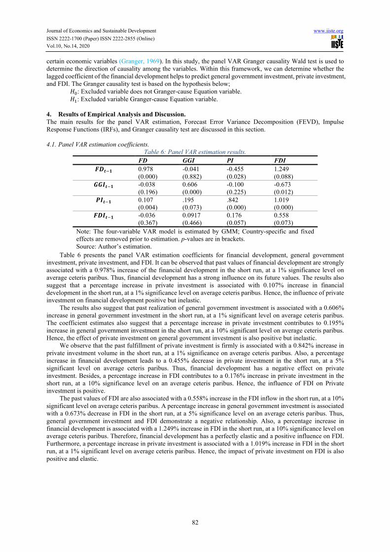
4.1. Panel VAR estimation coefficients.

Table 6: Panel VAR estimation results.

FD GGI PI FDI

789�: 0.978

(0.000)

-0.041

(0.882)

-0.455

(0.028)

1.249

(0.088)

;;<9�: -0.038

(0.196)

0.606

(0.000)

-0.100

(0.225)

-0.673

(0.012)

=<9�: 0.107

(0.004)

.195

(0.073)

.842

(0.000)

1.019

(0.000)

78<9�: -0.036

(0.367)

0.0917

(0.466)

0.176

(0.057)

0.558

(0.073)

Note: The four-variable VAR model is estimated by GMM; Country-specific and fixed

effects are removed prior to estimation. p-values are in brackets.

Source: Author’s estimation.

Table 6 presents the panel VAR estimation coefficients for financial development, general government

investment, private investment, and FDI. It can be observed that past values of financial development are strongly

associated with a 0.978% increase of the financial development in the short run, at a 1% significance level on

average ceteris paribus. Thus, financial development has a strong influence on its future values. The results also

suggest that a percentage increase in private investment is associated with 0.107% increase in financial

development in the short run, at a 1% significance level on average ceteris paribus. Hence, the influence of private

investment on financial development positive but inelastic.

The results also suggest that past realization of general government investment is associated with a 0.606%

increase in general government investment in the short run, at a 1% significant level on average ceteris paribus.

The coefficient estimates also suggest that a percentage increase in private investment contributes to 0.195%

increase in general government investment in the short run, at a 10% significant level on average ceteris paribus.

Hence, the effect of private investment on general government investment is also positive but inelastic.

We observe that the past fulfillment of private investment is firmly is associated with a 0.842% increase in

private investment volume in the short run, at a 1% significance on average ceteris paribus. Also, a percentage

increase in financial development leads to a 0.455% decrease in private investment in the short run, at a 5%

significant level on average ceteris paribus. Thus, financial development has a negative effect on private

investment. Besides, a percentage increase in FDI contributes to a 0.176% increase in private investment in the

short run, at a 10% significance level on an average ceteris paribus. Hence, the influence of FDI on Private

investment is positive.

The past values of FDI are also associated with a 0.558% increase in the FDI inflow in the short run, at a 10%

significant level on average ceteris paribus. A percentage increase in general government investment is associated

with a 0.673% decrease in FDI in the short run, at a 5% significance level on an average ceteris paribus. Thus,

general government investment and FDI demonstrate a negative relationship. Also, a percentage increase in

financial development is associated with a 1.249% increase in FDI in the short run, at a 10% significance level on

average ceteris paribus. Therefore, financial development has a perfectly elastic and a positive influence on FDI.

Furthermore, a percentage increase in private investment is associated with a 1.019% increase in FDI in the short

run, at a 1% significant level on average ceteris paribus. Hence, the impact of private investment on FDI is also

positive and elastic.



Vol.10, No.14, 2020

83

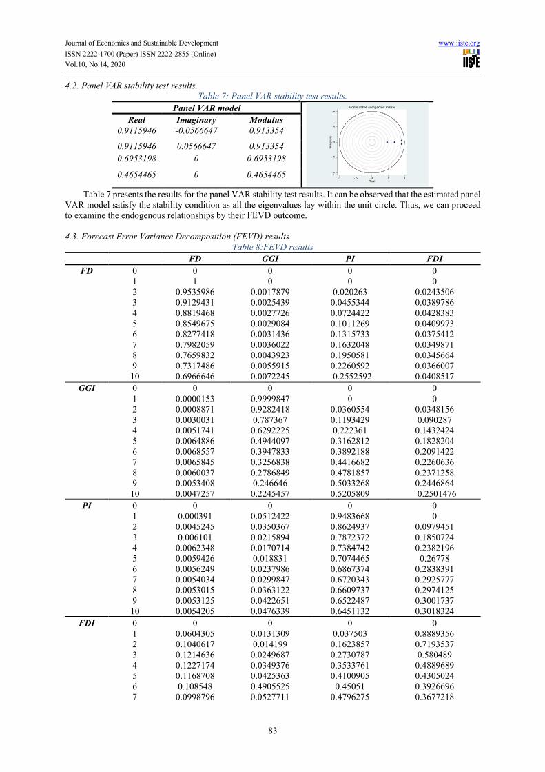
4.2. Panel VAR stability test results.

Table 7: Panel VAR stability test results.

Panel VAR model

Real Imaginary Modulus

0.9115946 -0.0566647 0.913354

0.9115946 0.0566647 0.913354

0.6953198 0 0.6953198

0.4654465 0 0.4654465

Table 7 presents the results for the panel VAR stability test results. It can be observed that the estimated panel

VAR model satisfy the stability condition as all the eigenvalues lay within the unit circle. Thus, we can proceed

to examine the endogenous relationships by their FEVD outcome.

4.3. Forecast Error Variance Decomposition (FEVD) results.

Table 8:FEVD results

FD GGI PI FDI

FD 0 0 0 0 0

1 1 0 0 0

2 0.9535986 0.0017879 0.020263 0.0243506

3 0.9129431 0.0025439 0.0455344 0.0389786

4 0.8819468 0.0027726 0.0724422 0.0428383

5 0.8549675 0.0029084 0.1011269 0.0409973

6 0.8277418 0.0031436 0.1315733 0.0375412

7 0.7982059 0.0036022 0.1632048 0.0349871

8 0.7659832 0.0043923 0.1950581 0.0345664

9 0.7317486 0.0055915 0.2260592 0.0366007

10 0.6966646 0.0072245 0.2552592 0.0408517

GGI 0 0 0 0 0

1 0.0000153 0.9999847 0 0

2 0.0008871 0.9282418 0.0360554 0.0348156

3 0.0030031 0.787367 0.1193429 0.090287

4 0.0051741 0.6292225 0.222361 0.1432424

5 0.0064886 0.4944097 0.3162812 0.1828204

6 0.0068557 0.3947833 0.3892188 0.2091422

7 0.0065845 0.3256838 0.4416682 0.2260636

8 0.0060037 0.2786849 0.4781857 0.2371258

9 0.0053408 0.246646 0.5033268 0.2446864

10 0.0047257 0.2245457 0.5205809 0.2501476

PI 0 0 0 0 0

1 0.000391 0.0512422 0.9483668 0

2 0.0045245 0.0350367 0.8624937 0.0979451

3 0.006101 0.0215894 0.7872372 0.1850724

4 0.0062348 0.0170714 0.7384742 0.2382196

5 0.0059426 0.018831 0.7074465 0.26778

6 0.0056249 0.0237986 0.6867374 0.2838391

7 0.0054034 0.0299847 0.6720343 0.2925777

8 0.0053015 0.0363122 0.6609737 0.2974125

9 0.0053125 0.0422651 0.6522487 0.3001737

10 0.0054205 0.0476339 0.6451132 0.3018324

FDI 0 0 0 0 0

1 0.0604305 0.0131309 0.037503 0.8889356

2 0.1040617 0.014199 0.1623857 0.7193537

3 0.1214636 0.0249687 0.2730787 0.580489

4 0.1227174 0.0349376 0.3533761 0.4889689

5 0.1168708 0.0425363 0.4100905 0.4305024

6 0.108548 0.4905525 0.45051 0.3926696

7 0.0998796 0.0527711 0.4796275 0.3677218



Vol.10, No.14, 2020

84

FD GGI PI FDI

8 0.0917931 0.0564682 0.500746 0.3509926

9 0.0846407 0.0596325 0.5161066 0.3396201

10 0.0785003 0.0624218 0.5272737 0.3318042

Table 8 presents the FEVD results for the dependent variables based on the panel VAR estimates. The FEVD

for financial development reaffirms that the it is strongly endogenous to its future values. Also, 25 % of the total

variance in financial development is explained by a shock to private investment. Thus, the FEVD reveals that

private investment is weakly endogenous to financial development. Furthermore, FDI explains 4% of the total

variance in financial development, indicating a strong exogenous relationship between the two variables. Similarly,

general government investment’s contribution to financial development is not significantly different from zero,

indicating a strong exogenous relationship.

The FEVD for general government investment shows that it is strongly endogenous to its future values in the

short run but exhibits a weak influence on itself in the long run. We also observe that 52 % of the total variance in

general government investment occurs as a result of a shock to private investment. Thus, private investment

exhibits a strong influence on future values of general government investment. Similarly, 25 % of the total variance

in general government investment occurs as a result of a shock to FDI. Hence FDI also exhibits a strong influence

on General government investment. The results also suggest that the proportion of variance in general government

investment explained by financial development is not significantly different from zero. Thus, financial

development exhibits a strong exogenous relationship with general government investment.

The private investment FEVD shows that private investment has a strong endogenous effect on its future

realizations. The results also reveal that 30 % of the total variance in private investment is explained by FDI. Hence,

FDI has a robust endogenous influence on private investment. We can also observe that general government

investment and financial development exhibit a strong exogenous effect on private investment, indicating that they

have a weak influence on the future realizations of private investment.

FDI exhibits a strong endogenous effect on its future values in the short run but shows a weak influence in

the long run. Private investment exhibits a strong influence on FDI as it explains 52 % of the total variance in FDI.

We also observe that Financial development and General government explain 7% and 6% of the total variance in

FDI, respectively, indicating that they have a robust exogenous relationship with FDI.

4.4. Impulse response functions.

Figure 1 presents the IRFs results, the accumulated response to a shock to financial development are summarized

as follows:

1. A negative shock to financial development causes private investment to decrease slightly.

2. A negative shock to financial development causes general government investment to increase slightly

in the short run.

3. A negative shock to financial development causes a slight increase in FDI but gradually decrease in

the long run.

The response of financial development to impulse from general government investment, private investment,

and FDI are summarized as follows:

1. A negative shock to General government investment has an insignificant effect on financial

development.

2. A shock to Private investment causes financial development to increase.

3. A shock to FDI inflow causes financial development to increase slightly in the short run but decreases

in the long run.

The IRFs are advantageous, in that, we can observe the type of shock to a variable and also observe the

accumulated responses from the variable. For example, we can observe that the effect of financial development on

the other dependent variables is due to a negative shock in the IRFs. Furthermore, the associated confidence

interval is helpful in determining the level of certainty for each response. Thus, the widening confidence interval

for each the response indicates that the long run effects shown in the IRFs are less specific.



Vol.10, No.14, 2020

85

Figure 1 Impulse response function.

4.5. Granger causality test results.

The Granger causality test is a useful panel data technique to determine whether one variable is useful for

predicting another variable. Thus, results from the Granger causality test provides robustness to the panel VAR

estimates. We discuss the causality between financial development and each form of investment in this subsection.

4.5.1. Pair-wise comparison of financial development and general government investment.

According to Table 9, the P-value for the causality from general government investment to financial development

is not significant at a 10% significance level, so we accept the null hypothesis that general government investment

does not Granger cause financial development. Likewise, the P-value for the causality from financial development

to general government investment is also not significant at a 10% significance level, so we accept the null

hypothesis that financial development does not Granger cause general government investment. Hence, there is no

causality between the two variables.

4.5.2. Pair-wise comparison of Financial development and Private investment.

According to Table 9, the P-value for the causality from private investment to financial development is significant

at a 1% significance level. Hence, we reject the null hypothesis and accept the alternative hypothesis that private

investment Granger causes financial development index. Also, the P-value for the causality from financial

development to private investment is significant at a 5% significance level so, we can reject the null hypothesis

and accept the alternative hypothesis that financial development Granger causes Private investment. Hence, there

is bilateral causality between the two variables.

4.5.3. Pair-wise comparison of Financial development and FDI.

According to Table 9, the P-value for the causality from FDI to financial development is not significant at a 10%

significance level, so we accept the null hypothesis that FDI does not Granger cause financial development. The

P-value for the causality from the financial development to FDI is significant at a 10% significance level, so we

can reject the null hypothesis and accept the alternative hypothesis that financial development Granger causes FDI.

Hence, there is a unilateral causality from financial development index to FDI.

4.5.4. Pair-wise comparison of financial development, general government investment, private investment, and

FDI.

According to Table 9, the P-value for the joint causality from general government investment, private investment,

and FDI to financial development is significant at 1% significance level, so we reject the null hypothesis and accept

the alternative hypothesis that General government investment, private investment, and FDI jointly Granger cause

financial development.



Vol.10, No.14, 2020

86

Table 9: Granger causality test results.

Chi2 df Prob>chi2

FD GGI 1.675 1 0.196

PI 8.420 1 0.004***

FDI 0.815 1 0.367

ALL 13.975 3 0.003***

GGI FD 0.022 1 0.882

FDI 0.532 1 0.466

PI 3.206 1 0.073*

ALL 21.556 3 0.000***

PI FD 4.834 1 0.028**

FDI 3.620 1 0.057*

GGI 1.474 1 0.225

ALL 5.007 3 0.171

FDI FD 2.903 1 0.088*

GGI 6.288 1 0.012**

PI 17.329 1 0.000***

ALL 25.357 3 0.000***

Note: ***, **, and * represents the rejection of the null hypothesis at 1% and 5%

and 10% level of significance respectively.

4.6. Discussions.

This study examines the dynamic relationship between financial development and investment in sub-Saharan

African countries using the Financial development index as the measure of how development the financial

institutions and financial markets are in sub-Saharan Africa. The major findings relating to our objective are

summarized in Table 10.

Table 10: Summary of findings on FD, GGI, PI, FDI.

FD to GII GII to FD FD to PI PI to FD FD to FDI FDI to FD

Level of

endogeneity

Strongly

exogenous

Strongly

exogenous

Strongly

exogenous

Weakly

endogenous

Strongly

exogenous

Strongly

exogenous

Direction of

endogeneity

None None Negative Positive Positive None

Causality None None Bilateral unilateral None

The findings from this study provide evidence that there is no endogenous relationship between financial

development and general government investment within sub-Saharan African countries. This finding could reflect

how local governments generates funding for infrastructural development in sub-Saharan Africa since many

countries within the subregion often depend on loans from external sources and international donor countries.

Consequently, local financial institutions often do not play a significant role in financing public infrastructural

development. Furthermore, it is also possible that local governments are less involved in the development of their

financial sectors by way of investment through partnerships, funding, and the provision of incentives that promote

the financial development in their economies.

The study also reveals that financial development has a negative influence on private investment due to an

adverse shock. As already mentioned in the introduction section of this study, financial development in sub-

Saharan African has regressed for decades, consequently, financial development has had detrimental effects on

private investment in the subregion leading to economic stagnation and widespread poverty. The recent

development in the financial sector due to the adoption of FinTech is helping to turn this negative tide and also

promote investment. Jack and Suri (2011) explain that timely money transfers, through financial technology such

as mobile money, enable households to smooth their consumption and make more effective investment decisions

in Sub-Saharan Africa.

Furthermore, the results suggest that private investment has a positive influence on financial development.

Thus, Private investment provides financial institutions and financial markets the avenues to expand their profits

through loans and other financial instruments, which also helps them to embrace innovation and improve their

services. Also, evidence from Granger causality suggests that the causal relationship between financial

development and Private investment is bilateral. This finding concurs with the opinion of some proponents of the

endogenous finance-growth models (e.g., Greenwood and Smith, 1997), because an increase in investment volume

would lead to a rise in the demand for external financing, which also causes financial intermediaries to persuade

households to increase their savings.

The study also reveals that financial development has a positive effect on FDI. The finding concurs with



Vol.10, No.14, 2020

87

Desbordes and Wei (2017), which suggests that FDI source and destination countries' financial development

jointly stimulate FDI by directly increasing access to external finance and indirectly supporting the overall

economic activity. The role of FDI is still a bone of contention among many researchers. However, the success

story of China with regards to the influence of FDI on local economies is a good signal for many policymakers in

sub-Saharan Africa. Thus, promoting the private sector is a useful strategy to attract FDI inflow into sub-Saharan

Africa.

Table 11: Summary of findings on GGI, PI, FDI.

PI to GGI GGI to PI PI to FDI FDI to PI GGI to FDI FDI to

GGI

Level of

endogeneity

Strongly

endogenous

Strongly

exogenous

Strongly

endogenous

Strongly

endogenous

Strongly

exogenous

Weakly

endogenous

Direction of

endogeneity

Positive Negative Positive Positive Negative Positive

Direction of

causality

Unilateral

None Bilateral None Unilateral

Findings relating to the dynamic interactions among the different forms of investment are summarized in

Table 11. According to Table 11, private investment is strongly endogenous to general government investment.

Similarly, the Granger causality test results also indicate that private investment granger causes general

government investment. Furthermore, we observe from Table 11 that FDI also contributes positively to general

government investment. These findings show the impact of the private sector and multinational companies on

government revenues which enables governments to undertake developmental projects in their countries.

Furthermore, we observe that FDI contributes positively to general government investment.

Policymakers in sub-Saharan African countries often try to ensure that their economies are attractive and

fertile for multinational companies due to the anticipated positive effects FDI has on local industries and the gross

domestic product (GDP). This study also reveals the importance of the private sector for FDI inflow. Thus, it is

possible that an increase in Private investment indicates a high return on investment in an economy, which attracts

FDI and motivate governments to improve infrastructure in order to promote the investment environment.

Consequently, we observe a bilateral relationship between private investment and FDI in sub-Saharan Africa.

5. Conclusion

This study examined the dynamic relationship between financial development and investment in 31sub-Saharan

African countries for the period of 2000-2015 via the panel VAR estimation techniques. The study adopted the

Financial development index of the IMF and examined its endogenous relationship with private investment,

general government investment, and FDI.

The study reveals that is no causal relationship between financial development and general government

investment in sub-Saharan Africa. We also found that there is a bilateral causal relationship between financial

development and Private investment. However, we noticed that even though financial development is exogenous

to private investment, it contributes negatively to private investment in sub-Saharan Africa. The study further

shows that financial development has a positive influence on FDI. Also, FDI and private investment have a bilateral

endogenous relationship.

Our findings have some policy implications for countries in sub-Saharan Africa. We recommend that

policymakers should focus on promoting private sector development due to its ability to drive financial

development and attract FDI inflow, as revealed in this study. The influence of the private sector on government

revenue can also not be overlooked since an increase in revenue for the government would also boost public

infrastructural development.

References

Abzari, M., Zarei, F. and Esfahani, S. (2011), “Analyzing The Link between Financial Development and Foreign

Direct Investment among D-8 Group of Countries”, International Journal of Economics and Finance, Vol.

3, available at: https://doi.org/10.5539/ijef.v3n6p148.

Aitken, B.J. and Harrison, A.E. (1999), “Do Domestic Firms Benefit from Direct Foreign Investment? Evidence

from Venezuela”, American Economic Review, Vol. 89 No. 3, pp. 605–618.

Anyanwu, J. (2011), Working Paper 135 - International Remittances and Income Inequality in Africa, No. 325,

African Development Bank, available at: https://ideas.repec.org/p/adb/adbwps/325.html (accessed 26

January 2020).

Asongu, S. (2014), “Linkages between Investment Flows and Financial Development: Causality Evidence from

Selected African Countries”, SSRN Electronic Journal, Vol. 5, pp. 269–299.

Basu, P. and Guariglia, A. (2007), “Foreign Direct Investment, inequality, and growth”, Journal of



Vol.10, No.14, 2020

88

Macroeconomics, Vol. 29 No. 4, pp. 824–839.

Bayar, Y. (2014), “DETERMINANTS OF FOREIGN DIRECT INVESTMENT INFLOWS IN THE

TRANSITION ECONOMIES OF EUROPEAN UNION”, No. 4, p. 6.

Beck, T.H.L., Levine, R. and Loayza, N. (2000), “Finance and the sources of growth”, Journal of Financial

Economics, Vol. 58 No. 1–2, pp. 261–300.

Caporale, G.M., Howells, P. and Soliman, A.M. (2005), “Endogenous Growth Models and Stock Market

Development: Evidence from Four Countries”, Review of Development Economics, Vol. 9 No. 2, pp. 166–

176.

Carp, L. (2012), “Can Stock Market Development Boost Economic Growth? Empirical Evidence from Emerging

Markets in Central and Eastern Europe”, Procedia Economics and Finance, Vol. 3, pp. 438–444.

Chaudhry, I., Malik, A. and Frooq, F. (2012), “Financial Liberalization and Macroeconomic Performance:

Empirical Evidence from Pakistan”, Finance and Management Sciences, Vol. 4.

Demetriades, P.O. and Hussein, K.A. (1996), “Does financial development cause economic growth? Time-series

evidence from 16 countries”, Journal of Development Economics, Vol. 51 No. 2, pp. 387–411.

Demirgüç-Kunt, A. and Levine, R. (2004), Financial Structure and Economic Growth: A Cross-Country

Comparison of Banks, Markets, and Development, MIT Press.

Desbordes, R. and Wei, S.-J. (2017), “The effects of financial development on foreign direct investment”, Journal

of Development Economics, Vol. 127, pp. 153–168.

Gebrehiwot, A., Esfahani, N. and Sayim, M. (2016), “The Relationship between FDI and Financial Market

Development: The Case of the Sub-Saharan African Region”, International Journal of Regional Development,

Vol. 3 No. 1, p. 64.

Gerschewski, S. (2013), “Do Local Firms Benefit from Foreign Direct Investment? An Analysis of Spillover

Effects in Developing Countries”, Asian Social Science, Vol. 9, pp. 67–76.

Goldsmith, R.W. (1969), Financial Structure and Development, Yale University Press, New Haven.

Granger, C.W.J. (1969), “Investigating Causal Relations by Econometric Models and Cross-spectral Methods”,

Econometrica, Vol. 37 No. 3, pp. 424–438.

Greenwood, J. and Smith, B.D. (1997), “Financial markets in development, and the development of financial

markets”, Journal of Economic Dynamics and Control, Vol. 21 No. 1, pp. 145–181.

Hamdi, H., Hakimi, A. and Sbia, R. (2013), “Multivariate Granger Causality between Financial Development,

Investment and Economic Growth: Evidence from Tunisia”, Journal of Quantitative Economics: Journal of

the Indian Econometric Society, Vol. 11.

INTERNATIONAL MONETARY FUND. (2016), Financial Development in Sub-Saharan Africa., INTL

MONETARY FUND, Place of publication not identified.

Jack, W. and Suri, T. (2011), Mobile Money: The Economics of M-PESA, No. w16721, National Bureau of

Economic Research, Cambridge, MA, p. w16721.

King, R.G. *Levine. (1993), Finance and Growth : Schumpeter Might Be Right, No. 1083, The World Bank,

available at: https://ideas.repec.org/p/wbk/wbrwps/1083.html (accessed 26 January 2020).

Levine, R. (1997), “Financial Development and Economic Growth: Views and Agenda”, Journal of Economic

Literature, Vol. 35 No. 2, pp. 688–726.

Levine, R. and Renelt, D. (1992), “A Sensitivity Analysis of Cross-Country Growth Regressions”, The American

Economic Review, Vol. 82 No. 4, pp. 942–963.

Levine, R. and Zervos, S. (1998), “Stock Markets, Banks, and Economic Growth”, The American Economic

Review, Vol. 88 No. 3, pp. 537–558.

Love, I. and Zicchino, L. (2006), “Financial development and dynamic investment behavior: Evidence from panel

VAR”, The Quarterly Review of Economics and Finance, Vol. 46 No. 2, pp. 190–210.

Lütkepohl, H. (2005), New Introduction to Multiple Time Series Analysis, Springer-Verlag, Berlin Heidelberg,

available at:https://doi.org/10.1007/978-3-540-27752-1.

Mello, L.R. de. (1997), “Foreign direct investment in developing countries and growth: A selective survey”, The

Journal of Development Studies, Vol. 34 No. 1, pp. 1–34.

Muyambiri, B. (2016), “THE SEQUENCING OF FINANCIAL REFORMS AND BANK-BASED FINANCIAL

DEVELOPMENT IN MAURITIUS”, Journal of Accounting and Management, Vol. 6 No. 1, pp. 89–114.

Muyambiri, B. and Odhiambo, N.M. (2017), The Causal Relationship between Financial Development and

Investment in Botswana, No. 22607, University of South Africa, Department of Economics, available at:

https://ideas.repec.org/p/uza/wpaper/22607.html (accessed 26 January 2020).

Nasser, O.M. and Gomez, X.G. (2009), “Do well-functioning financial systems affect the FDI flows to latin

america?”, Vol. 1, pp. 60–75.

Pagano, M. (1993), “Financial markets and growth: An overview”, European Economic Review, Vol. 37 No. 2,

pp. 613–622.

Pedroni, P. (1999), “Critical Values for Cointegration Tests in Heterogeneous Panels with Multiple Regressors”,



Vol.10, No.14, 2020

89

Oxford Bulletin of Economics and Statistics, Vol. 61 No. S1, pp. 653–670.

Pesaran, M.H. (2004), General Diagnostic Tests for Cross Section Dependence in Panels, SSRN Scholarly Paper

No. ID 572504, Social Science Research Network, Rochester, NY, available at:

https://papers.ssrn.com/abstract=572504 (accessed 26 January 2020).

Pesaran, M.H. (2007), “A simple panel unit root test in the presence of cross-section dependence”, Journal of

Applied Econometrics, Vol. 22 No. 2, pp. 265–312.

Rousseau, P.L. and Vuthipadadorn, D. (2005), “Finance, investment, and growth: Time series evidence from 10

Asian economies”, Journal of Macroeconomics, Vol. 27 No. 1, pp. 87–106.

Rousseau, P.L. and Wachtel, P. (2011), “What Is Happening to the Impact of Financial Deepening on Economic

Growth?”, Economic Inquiry, Vol. 49 No. 1, pp. 276–288.

Sahay, R., [email protected], Cihak, M., [email protected], N’Diaye, P., PN’[email protected], Barajas, A., et al.

(2015), “Financial Inclusion: Can it Meet Multiple Macroeconomic Goals?”, Staff Discussion Notes, Vol. 15

No. 17, p. 1.

Sahin, S. and Ege, I. (2015), “Financial Development and FDI in Greece and Neighbouring Countries: A Panel

Data Analysis”, Procedia Economics and Finance, Vol. 24, pp. 583–588.

Sakyi, D., Kofi Boachie, M. and Immurana, M. (2016), “Does Financial Development Drive Private Investment

in Ghana?”, Economies, Vol. 4 No. 4, p. 27.

Svirydzenka, K. and [email protected]. (2016), “Introducing a New Broad-based Index of Financial

Development”, IMF Working Papers, Vol. 16 No. 05, p. 1.

Todo, Y. (2003), “Empirically consistent scale effects: An endogenous growth model with technology transfer to

developing countries”, Journal of Macroeconomics, Vol. 25 No. 1, pp. 25–46.

A Study on the Dynamic Relationship Between Financial ...

Documents

Transcript of A Study on the Dynamic Relationship Between Financial ...