i

A STUDY ON THE CONCENTRATION AND DISPERSION OF PM10 IN UTHM BY

USING SIMPLE MODELLING AND METEOROLOGICAL FACTORS

MALEK FAIZAL B ABD RAHMAN

A Project Report submitted in partial

fulfilment of the requirements for the award of the

Degree of Master of Engineering in Civil Engineering

Faculty of Civil and Environmental Engineering

Universiti Tun Hussein Onn Malaysia

FEBRUARY, 2013

v

ABSTRACT

Air pollution is the introduction of chemicals, particulate matter, or biological materials that

cause harm or discomfort to humans or other living organisms, or cause damage to the natural

environment or built environment, into the atmosphere. Air pollution can also be known as

degradation of air quality resulting from unwanted chemicals or other materials occurring in

the air. The simple way to know how polluted the air is to calculate the amounts of foreign

and/or natural substances occurring in the atmosphere that may result in adverse effects to

humans, animals, vegetation and/or materials. The objective of this study is to create a

simulation of air quality dispersion in UTHM campus by using computer aided design

mechanism such as software and calculating tools. Another objective is to compare the

concentration obtained from the end result of calculation with past studies. The air pollutant in

the scope of study is Particulate Matter (PM10). The highest reading recorded for E-Sampler

was 305µg/m3. It was recorded in Structure Lab sampling point while the highest expected

concentration by the Gaussian Dispersion Model was 184µg/m3 for UTHM Stadium. The

recommended value for permissible exposure to particulate matter in 24 hours time is

150µg/m3 according to the Recommended Malaysian Air Quality Guidelines.

vi

ABSTRAK

Pencemaran udara adalah pengenalan bahan kimia, bahan zarahan atau bahan biologi yang

boleh menyebabkan mudarat atau ketidakselesaan kepada manusia atau organisma hidup lain,

atau menyebabkan kerosakan kepada persekitaran semulajadi atau alam bina, ke

atmosfera.Pencemaran udara juga boleh dikenali sebagai degradasi kualiti udara yang terhasil

dari bahan kimia yang tidak diingini atau bahan-bahan lain yang berlaku di udara. Cara

mudah untuk mengetahui bagaimana tercemar udara untuk mengira jumlah bahan-bahan asing

dan / atau semula jadi yang berlaku dalam suasana yang mungkin menyebabkan kesan buruk

kepada manusia, haiwan, tumbuh-tumbuhan dan / atau bahan-bahan. Objektif kajian ini

adalah untuk mewujudkan simulasi penyebaran kualiti udara di kampus UTHM dengan

menggunakan bantuan model komputer seperti perisian dan alat pengiraan. Objektif lain

adalah untuk membandingkan kepekatan yang diperolehi daripada hasil akhir pengiraan

dengan kajian lepas. Pencemar udara di dalam skop kajian ini adalah Zarah Halus 10 micron

(PM10). Nilai bacaan tertinggi yang dicatatkan untuk E-Sampler adalah 305μg/m3. Ia telah

direkodkan di dalam kawasan Makmal Struktur manakala nilai kepekatan tertinggi yang

dijana oleh Model Serakan Gaussian adalah 184μg/m3 untuk UTHM Stadium. Nilai yang

disyorkan untuk pendedahan yang dibenarkan untuk zarah halus dalam tempoh masa 24 jam

adalah 150μg/m3 mengikut kepada Garis Panduan Saranan Kualiti Udara Malaysia.

vii

TABLE OF CONTENTS

CHAPTER ITEM PAGE

THESIS STATUS APPROVAL FORM

TITLE PAGE i

DECLARATION ii

DEDICATION iii

ACKNOWLEDGEMENT iv

ABSTRACT v

ABSTRAK vi

TABLE OF CONTENTS vii

LIST OF TABLES xii

LIST OF FIGURES xiii

LIST OF EQUATIONS xv

LIST OF APPENDICES xvi

CHAPTER I INTRODUCTION 1

1.1 Introduction 1

1.2 Research Objective 2

1.3 Research Scope 2

1.4 Problem Statement 3

1.5 Research Significant 3

viii

CHAPTER II LITERATURE REVIEW 4

2.1 Introduction 4

2.2 Meteorological Aspect for Air Pollution 5

2.2.1 Effects of Atmospheric Pressure 5

in Air Pollution

2.2.2 Effects of Topography in Air Pollution 8

2.2.3 Effects of Temperature Inversion 9

2.2.3.1 Causes of Temperature Inversions 9

2.2.3.2 Consequences of Temperature 11

Inversions

2.2.4 Effects of Wind Speed and Wind Direction 12

in Air Pollution

2.3 Characteristics of Air Quality in Malaysia 13

2.4 Air Pollution Studies in Malaysia 16

2.5 Sources of Air Pollution from Certain Industries in 18

Malaysia

2.6 Particulate Matter 21

2.6.1 Particulate Matter Impacts 22

2.6.1.1 Particulate Matter Impact on 23

Humans Health

2.6.1.2 Particulate Matter Impact on 23

Environments

2.6.2 Particulate Matter Studies in Malaysia 24

2.7 Air Quality Dispersion Model 25

2.7.1 Box Model 26

2.7.2 Gaussian Model 26

2.7.3 Lagrangian Model 27

2.7.4 Eulerian Model 27

2.7.5 Dense Gas Model 27

2.8 Atmospheric Stability 28

2.8.1 Dry Adiabatic 28

2.8.2 Wet Adiabatic 29

2.8.3 Environmental Lapse Rate 30

ix

2.8.4 Unstable Conditions 32

2.8.5 Neutral Conditions 33

2.8.6 Stable Conditions 34

2.9 Stability Classes 35

2.10 Stability and Plume Behaviours 38

2.10.1 Looping Plume 38

2.10.2 Fanning Plume 39

2.10.3 Coning Plume 39

2.10.4 Lofting Plume 40

2.10.5 Fumigating Plume 41

CHAPTER III METHODOLOGY 43

3.1 Introduction 43

3.2 Flowchart of Methodology 44

3.3 Title Acquisition and Confirmation 45

3.4 Literature Review 45

3.5 Methodology 46

3.5.1 Site Investigation inside Universiti Tun 46 Hussein

Onn Malaysia

3.5.2 Data Collection and Compilation 50

3.5.2.1 Data Collection 50

3.5.2.2 E-Sampler 50

3.5.2.3 Data Calculation 54

3.6 Air Quality Modelling Using Gaussian 55

Dispersion Model

3.7 Air Quality Standards 60

CHAPTER IV DATA ANALYSIS 62

4.1 Introduction 62

4.2 Characteristic of Particulate Concentration 63

x

4.3 Analysis of Particulate Matter 10µm 64

(PM10) in Filter Paper by Location

4.3.1 PM10 Concentration at Structure 64

Laboratory

4.3.2 PM10 Concentration at 65

UTHM Stadium

4.3.3 PM10 Concentration at 65

Tun Dr Ismail Residential College

4.4 Graphical Analysis of PM10 Concentration 66

4.4.1 E-Sampler 67

4.4.1.1 PM10 Concentration at 67

Structure Laboratory

4.4.1.2 PM10 Concentration at 68

UTHM Stadium

4.4.1.3 PM10 Concentration at 69

Tun Dr Ismail

Residential College

4.4.1.4 Overall Concentration of 70

PM10 for E-Sampler

4.4.2 Gaussian Dispersion Model 72

4.4.2.1 PM10 Concentration at 72

Structure Laboratory

4.4.2.2 PM10 Concentration at 72

UTHM Stadium

4.4.2.3 PM10 Concentration at 75

Tun Dr Ismail

Residential College

4.4.2.4 Distribution of PM10 77

Concentration from

Gaussian Dispersion Model

4.5 Summary of Data Analysis 78

xi

CHAPTER V CONCLUSION AND RECOMMENDATION 80

5.1 Conclusion 80

5.2 Recommendation 82

REFERENCE 84

APPENDICES 89

xii

LIST OF TABLE

2.1 The Malaysia Air Pollution Index 15

2.2 The ambient air quality standards for Malaysia and the United States 15

2.3 Stack Gas Emission Standards 18

2.4 Pasquill and Gifford Stability Classes 35

2.5 Stability Class Details 36

3.1 Constants in Empirical Relationship for σy and σz 59

3.2 Recommended Malaysian Air Quality Guidelines (RMAQG) 60

3.3 United States Environmental Protection Agency Standards 60

3.4 World Health Organization Air Quality Guidelines for 61

Particulate Matter, Ozone, Nitrogen Dioxide and Sulphur Dioxide

4.1 Characteristics of Particulate Matter Concentration on 4 Sampling Point 63

4.2 Results of PM10 Concentration at Structure Laboratory 64

4.3 Results of PM10 Concentration at UTHM Stadium 65

4.4 Results of PM10 Concentration at Tun Dr Ismail Residential College 66

4.5 E-Sampler and Gaussian Dispersion Model Result Comparison 79

xiii

LIST OF FIGURES

2.1 Standard Atmospheric Density Based on Elevation 6

2.2 Air Pollution Sources and Means of Dispersion 7

2.3 Temperature Inversion and the Effects 11

2.4 Comparison of Size between Particulates with Human Hair 22

and Sand

2.5 Annual Average Concentration of Particulate Matter (PM10), 25

1996 – 2004

2.6 Dry Adiabatic Lapse Rate 29

2.7 Wet Adiabatic Lapse Rate 30

2.8 Environmental Lapse Rate 31

2.9 Unstable Conditions 32

2.10 Neutral Conditions 33

2.11 Stable Conditions 34

2.12 Looping Plume 38

2.13 Fanning Plume 39

2.14 Coning Plume 40

2.15 Lofting Plume 41

2.16 Fumigating Plume 42

3.1 The Study Area Aerial View from Google Earth 46

3.2 Compass Bearing and Direction Based on UTHM Campus 47

3.3 Tun Dr Ismail Residential College 47

3.4 Point Source Viewed from Tun Dr Ismail Residential College 48

3.5 Structure Laboratory 48

3.6 Smoke Stack Viewed from Structure Laboratory 49

3.7 UTHM Stadium 49

xiv

3.8 E-Sampler 51

3.9 E-Sampler Control Panel 51

3.10 E-Sampler Wind Speed and Wind Direction Combination 52

3.11 E-Sampler Sharp Cut Cyclone and Rain Cap 52

3.12 Light Scatter by Airborne Particulate in the E-Sampler 53

3.13 Gaussian Dispersion Model Plume Visualization 56

3.14 σy Variation with Downwind Distance x 57

3.15 σz Variation with Downwind Distance x 58

4.1 Concentration VS Wind Speed for Structure Laboratory 67

4.2 Concentration VS Wind Speed for UTHM Stadium 68

4.3 Concentration VS Wind Speed for Tun Dr Ismail Residential College 69

4.4 Comparison of Concentration for All Sites 71

4.5 Concentration VS Wind Speed for Structure Laboratory 73

4.6 Concentration VS Wind Speed for UTHM Stadium 74

4.7 Concentration VS Wind Speed for Tun Dr Ismail Residential College 76

4.8 Overall Concentration Distribution of PM10 77

xv

LIST OF EQUATIONS

3.1 PM10 calculation 54

3.2 Volume calculation 54

3.3 Gaussian Dispersion Model Equation 55

3.4 Approximation of σy 58

3.5 Approximation of σz 58

xvi

LIST OF APPENDICES

Appendix A (Data from E-Sampler for Structure Lab, Week 1)

Appendix B (Data from E-Sampler for Structure Lab, Week 2)

Appendix C (Data from E-Sampler for Structure Lab, Week 3)

Appendix D (Data from E-Sampler for Structure Lab, Week 4)

Appendix E (Data from E-Sampler for UTHM Stadium, Week 1)

Appendix F (Data from E-Sampler for UTHM Stadium, Week 2)

Appendix G (Data from E-Sampler for UTHM Stadium, Week 3)

Appendix H (Data from E-Sampler for UTHM Stadium, Week 4)

Appendix I (Data from E-Sampler for Tun Dr Ismail College, Week 1)

Appendix J (Data from E-Sampler for Tun Dr Ismail College, Week 2)

Appendix K (Data from E-Sampler for Tun Dr Ismail College, Week 3)

Appendix L (Data from E-Sampler for Tun Dr Ismail College, Week 4)

1

CHAPTER I

INTRODUCTION

1.1 Introduction

Air pollution is the introduction of chemicals, particulate matter, or biological

materials that cause harm or discomfort to humans or other living organisms, or

cause damage to the natural environment or built environment, into the atmosphere.

The atmosphere is a complex dynamic natural gaseous system that is essential to

support life on planet Earth. Stratospheric ozone depletion due to air pollution has

long been recognized as a threat to human health as well as to the Earth's ecosystems.

Indoor air pollution and urban air quality are listed as two of the world‟s worst

pollution problems in the 2008 Blacksmith Institute World's Worst Polluted Places

report. (Blacksmith Institute, 2011)

The air we breathe contains particles and composition of particles, including

mineral dust, metals, metalloids, sea salt, nitrate and ammonium sulphate, organic

compounds, elemental carbon and organic and inorganic pollutants that live almost

entirely in the gas phase. Some of them are directly emitted into the atmosphere

either by natural sources and anthropogenic (primary particles), while others are the

result of homogeneous or heterogeneous nucleation and condensation of gases

(secondary particles) (Dongarrà, Manno et al. 2010).

2

Air quality is defined as a measure of the condition of air relative to the

requirements of one or more biotic species or to any human need or purpose.

(Johnson et al, 1997) while air quality indices (AQI) are numbers used by

government agencies to characterize the quality of the air at a given location. As the

AQI increases, an increasingly large percentage of the population is likely to

experience increasingly severe adverse health effects. To compute the AQI, it

requires an air pollutant concentration from a monitor or model. The function used to

convert from air pollutant concentration to AQI varies by pollutant, and is different

in different countries.

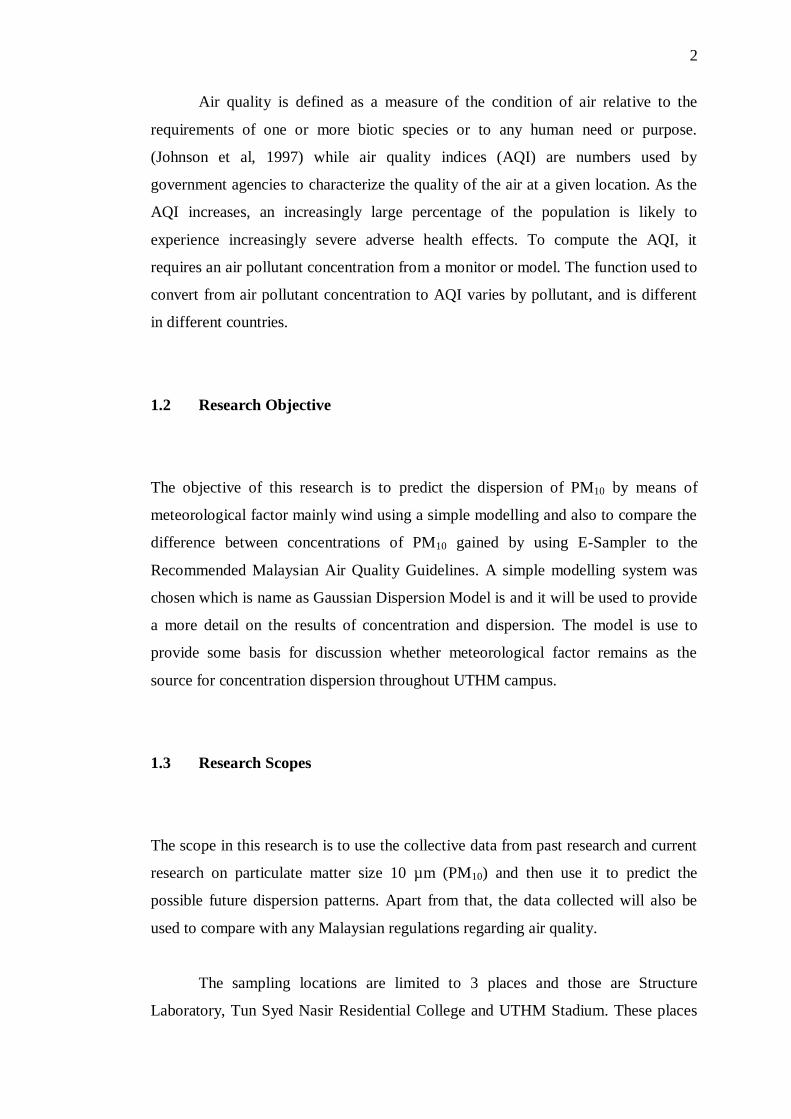
1.2 Research Objective

The objective of this research is to predict the dispersion of PM10 by means of

meteorological factor mainly wind using a simple modelling and also to compare the

difference between concentrations of PM10 gained by using E-Sampler to the

Recommended Malaysian Air Quality Guidelines. A simple modelling system was

chosen which is name as Gaussian Dispersion Model is and it will be used to provide

a more detail on the results of concentration and dispersion. The model is use to

provide some basis for discussion whether meteorological factor remains as the

source for concentration dispersion throughout UTHM campus.

1.3 Research Scopes

The scope in this research is to use the collective data from past research and current

research on particulate matter size 10 µm (PM10) and then use it to predict the

possible future dispersion patterns. Apart from that, the data collected will also be

used to compare with any Malaysian regulations regarding air quality.

The sampling locations are limited to 3 places and those are Structure

Laboratory, Tun Syed Nasir Residential College and UTHM Stadium. These places

3

are selected because of the distance factor and also the impact it may cause for a

highly concentrated area.

1.4 Problem Statements.

In Malaysia, there are no ambient air quality standards but the Malaysian government

however established ambient air quality guidelines in 1988 (Department of

Environment, 2012). Pollutants addressed in the guidelines include ozone, carbon

monoxide, nitrogen dioxide, sulphur dioxide, total suspended particles, particulate

matter under 10 microns, lead and dust fall. The averaging time which varies from 1

to 24 hours for different air pollutants in the Recommended Malaysian Air Quality

Guidelines represents the period of time over which measurements is monitored and

reported for the assessments of human health impacts of specific air pollutants.

Universiti Tun Hussein Onn Malaysia (UTHM) is located in a unique area

because it is surrounded by industrial area which emits pollutants directly into the

air. There have been cases; but it is not reported as formal reports, more on visual

reports; where particulate matters released from the industrials area goes up in the air

and then for some reason fall down back to earth like snow and it accumulate on the

ground surface. For this reason, people in the UTHM compound are always in

questions with their health when they encounter any sickness whether it is caused by

the long exposure to pollutants emitted by the factories or because of some other

factors.

1.5 Research Significant

This thesis will provide knowledge about the dispersion of pollutant mainly

particulate matters fewer than 10 microns by looking further into the meteorological

factors. Furthermore, this research is hopefully to help others in their search for the

best system to use in the future.

4

CHAPTER II

LITERATURE REVIEW

2.1 Introduction

Air pollution can also be known as degradation of air quality resulting from

unwanted chemicals or other materials occurring in the air. The simple way to know

how polluted the air is to calculate the amounts of foreign and/or natural substances

occurring in the atmosphere that may result in adverse effects to humans, animals,

vegetation and/or materials. Urban air pollution with its long and short term impacts

on human health, well – being and the environment has been a widely recognized

problem over the last 50 years (Gurjar et al. 2008; Ozden et al. 2008). In addition to

population growth, the rapid growth of urbanization and industrialization; where the

progressive expansion of suburbs into closer proximity with industrial facilities in

certain areas has led to the problem of air pollution becoming an increasingly

important issue (Ferger 1999; Molina and Molina 2004). Besides deleterious effects

on human health, air pollution can negatively impact ecosystems, materials,

buildings and works of art, vegetations and visibility (Ilyas et al. 2009; Mage et al.

1996; Riga-Karandinos and Saitanis, 2005).

5

2.2 Meteorological Aspect for Air Pollution

The transport and dispersion of air pollutants in the ambient air are influenced by

many complex factors. Global and regional weather patterns and local topographical

conditions affect the way that pollutants are transported and dispersed. The amount

and kind of pollutants that are released into the air play a major role in determining

the degree of air pollution in a specific area. However, other factors are involved,

mainly:

1. Atmospheric pressure;

2. Topography or earth surfaces;

3. Temperature inversion;

4. Wind speed and wind direction

2.2.1 Effects of Atmospheric Pressure in Air Pollution

Atmospheric pressure is the force per unit area exerted into a surface by the weight of

air above that surface in the atmosphere of Earth. In most circumstances atmospheric

pressure is closely approximated by the hydrostatic pressure caused by the mass of air

above the measurement point. Low-pressure areas have less atmospheric mass above

their location, whereas high-pressure areas have more atmospheric mass above their

location. Likewise, as elevation increases, there is less overlying atmospheric mass,

so that pressure decreases with increasing elevation. On average, a column of air one

square centimetre in cross-section, measured from sea level to the top of the

atmosphere, has a mass of about 1.03 kg and weight of about 10.1 N. The difference

in atmospheric pressure and density varies widely on Earth as can be clearly seen in

Figure 2.1 while Figure 2.2 will show the atmospheric composition from the ground

surface.

6

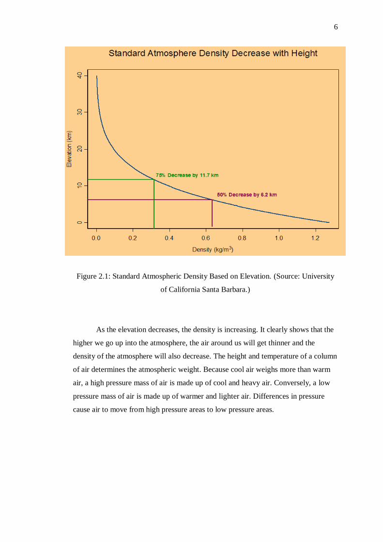
Figure 2.1: Standard Atmospheric Density Based on Elevation. (Source: University

of California Santa Barbara.)

As the elevation decreases, the density is increasing. It clearly shows that the

higher we go up into the atmosphere, the air around us will get thinner and the

density of the atmosphere will also decrease. The height and temperature of a column

of air determines the atmospheric weight. Because cool air weighs more than warm

air, a high pressure mass of air is made up of cool and heavy air. Conversely, a low

pressure mass of air is made up of warmer and lighter air. Differences in pressure

cause air to move from high pressure areas to low pressure areas.

7

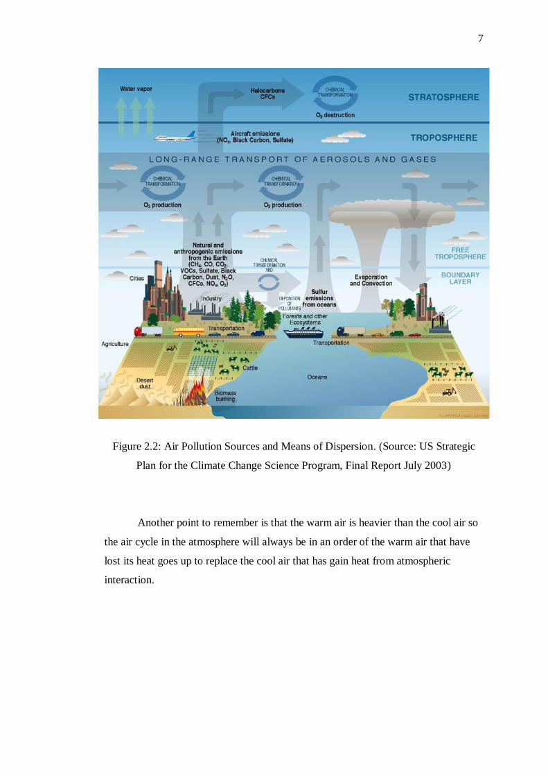
Figure 2.2: Air Pollution Sources and Means of Dispersion. (Source: US Strategic

Plan for the Climate Change Science Program, Final Report July 2003)

Another point to remember is that the warm air is heavier than the cool air so

the air cycle in the atmosphere will always be in an order of the warm air that have

lost its heat goes up to replace the cool air that has gain heat from atmospheric

interaction.

8

2.2.2 Effects of Topography in Air Pollution

Topography is a field of planetary science comprising the study of surface shape and

features of the Earth. It is also the description of such surface shapes and features

(especially their depiction in maps). The topography of an area can also mean the

surface shape and features. Topography also means the arrangement of the natural

and artificial physical features of an area. Topography specifically involves the

recording of relief or terrain, the three-dimensional quality of the surface, and the

identification of specific landforms.

Terrain, or land relief, is the vertical and horizontal dimension of land

surface. Terrain is used as a general term in physical geography, referring to the lay

of the land. This is usually expressed in terms of the elevation, slope, and orientation

of terrain features. Terrain affects surface water flow and distribution. Over a large

area, it can affect weather and climate patterns.

In terms of terrain, mountain areas are generally colder than surrounding land

due to higher altitudes. Mountainous regions block the flow of air masses, which rise

to pass over the higher terrain. The rising air is cooled, which causes condensation of

water vapour, and precipitation. These being the case, one side of a mountain, the

windward side, will often have more precipitation and vegetation; the leeward side is

often drier.

In terms of proximity to the ocean, land and water retain different amounts of

heat. Land heats more quickly than water, but water holds heat longer. Proximity to

water moderates the climate, while inland climates are harsher. Those living near the

water will experience breezy, moist weather, when the warm air from the land meets

the cooler air from the water and rises, making for a windy climate with

precipitation. The further inland one goes, the drier the climate in most regions.

Concentrations of pollutants can be greater in valleys than for areas of higher

ground. This is because, under certain weather conditions, pollutants can become

trapped in low lying areas such as valleys. This happens for example, on still sunny

9

days when pollution levels can build up due to a lack of wind to disperse the

pollution. This can also happen on cold calm and foggy days during winter. If towns

and cities are surrounded by hills, wintertime smog‟s may also occur. Pollution from

vehicles, homes and other sources may become trapped in the valley, often following

a clear cloudless night. Cold air then becomes trapped by a layer of warmer air above

the valley (USEPA, 2011).

2.2.3 Effects of Temperature Inversion

The situation of having warm air on top of cooler air is referred to as a temperature

inversion, because the temperature profile of the atmosphere is “inverted” from its

usual state. Inversions layers can occur anywhere from close to ground level up to

thousands of feet into the atmosphere and because of that, there are two types of

temperature inversions:

1. Surface inversions that occur near the Earth‟s surface;

2. Aloft inversions that occur higher above the ground.

2.2.3.1 Causes of Temperature Inversions

The most common manner in which surface inversions form is through the cooling of

the air near the ground at night. Once the sun goes down, the ground loses heat very

quickly, and this cools the air that is in contact with the ground. However, since air is

a very poor conductor of heat, the air just above the surface remains warm.

Conditions that favour the development of a strong surface inversion are calm

winds, clear skies, and long nights. Calm winds prevent warmer air above the surface

from mixing down to the ground, and clear skies increase the rate of cooling at the

Earth‟s surface. Long nights allow for the cooling of the ground to continue over a

10

longer period of time, resulting in a greater temperature decrease at the surface. Since

the nights in the wintertime are much longer than nights during the summertime,

surface inversions are stronger and more common during the winter months. A

strong inversion implies a substantial temperature difference exists between the cool

surface air and the warmer air aloft. During the daylight hours, surface inversions

normally weaken and disappear as the sun warms the Earth‟s surface. However,

under certain meteorological conditions, such as strong high pressure over the area,

these inversions can persist as long as several days. In addition, local topographical

features can enhance the formation of inversions, especially in valley locations.

Surface temperature inversions play a major role in air quality, especially

during the winter when these inversions are the strongest. The warmer air above the

cooler air acts like a lid where it suppress, vertical mixing and trapping the cooler air

at the surface along with the pollutants because as pollutants from vehicles,

fireplaces, and industry are emitted into the air, the inversion traps these pollutants

near the ground, leading to poor air quality. Graphical ways of understanding

temperature inversion can be clearly seen in Figure 2.3.

11

Figure 2.3: Temperature Inversion and the Effects. (US Environmental Protection

Agency, 2011)

2.2.3.2 Consequences of Temperature Inversions

Some of the most significant consequences of temperature inversions are the extreme

weather conditions they can sometimes create. Although freezing rain,

thunderstorms, and tornadoes are significant weather events, one of the most

important things impacted by an inversion layer is smog. This is the brownish gray

haze that covers many of the world‟s largest cities and is a result of dust, auto

exhaust, and industrial manufacturing.

Smog is impacted by the inversion layer because it is in essence, capped,

when the warm air mass moves over an area. This happens because the warmer air

layer sits over a city and prevents the normal mixing of cooler, denser air. The air

12

instead becomes still and over time the lack of mixing causes pollutants to become

trapped under the inversion, developing significant amounts of smog.

During severe inversions that last over long periods, smog can cover entire

metropolitan areas and cause respiratory problems for the inhabitants of those areas.

London‟s Great Smog of 1952 and Mexico‟s similar problems are extreme examples

of smog being impacted by the presence of an inversion layer.

In December 1952, such an inversion occurred in London. Because of the

cold December weather at the time, Londoners began to burn more coal, which

increased air pollution in the city. Since the inversion was present over the city at the

same time, these pollutants became trapped and increased London‟s air pollution.

The result was the Great Smog of 1952 that was blamed for thousands of deaths.

Like London, Mexico City has also experienced problems with smog that have been

exacerbated by the presence of an inversion layer. This city is infamous for its poor

air quality but these conditions are worsened when warm sub-tropical high pressure

systems move over the city and trap air in the Valley of Mexico. When these

pressure systems trap the valley‟s air, pollutants are also trapped and intense smog

develops. Since 2000, Mexico's government has developed a ten year plan aimed at

reducing ozone and particulates released into the air over the city (USEPA, 2011).

2.2.4 Effects of Wind Speed and Wind Direction in Air Pollution

Wind is simply air in motion. On global or macro scale wind patterns are set up due

to unequal heating of earth surface by solar radiation at the equator and the Polar

Regions, rotation of the earth and the difference between conductive capacities of

land and ocean masses. Secondary or mesoscale circulation patterns develop because

of the regional or local topography. Mountain ranges, cloud cover, water bodies,

deserts, forestation, etc., influence wind patterns on scales of a few hundred

kilometres. Accordingly a pattern of wind is setup, some seasonal and some

permanent.

13

Micro scale phenomenon occurs over areas of less than 10 kilometres extent.

Standard wind patterns may deviate markedly due to varying frictional effects of the

earth surface, such as, rural open land, irregular topography and urban development,

effect of radiant heat from deserts and cities, effect of lakes, etc.

The movement of air at the mesoscale and micro scale levels is of concern in

control of air pollution. A study of air movement over relatively small geographical

regions can help in understanding the movement of pollutants.

The dispersion of air pollutants mainly depends on physical processes is air;

those of wind and weather. How far air pollutants are transported mainly depends

upon particle size of the compounds and at which height the pollution was emitted

into the air. Fumes that are emitted into air through high smoke stacks will mix with

air so that local concentrations are not very high. However, wind will transport the

particle compounds and the pollution will be spread and disperse where else, rain can

remove pollutants from air (USEPA, 2011).

2.3 Characteristics of Air Quality in Malaysia

In the early days of Malaysia, development and growth were not planned; they were

initiated according to the needs and pressures of the time. Consequently, this

haphazard development has resulted in negative impacts on the environment as a

whole and on air quality in particular (Sham, 1994). Earlier, Sham (1979) pointed out

that atmospheric pollution problem is becoming more serious as there is always a

potential for the occurrence of inversion in the valley. In anticipation of the potential

severity and magnitude of the problem, the government enacted into law the

Environmental Quality Act in 1974; subsequently, the Division of the Environment

was established and the Clean Air Regulations were formerly gazette in 1978.

The first “long-term” air quality monitoring project emphasizing suspended

particulate and sulphur dioxide was carried out by the Department of Environment

14

(DOE) and the Meteorological Service Department (MMS) at the industrial and

residential zones in Petaling Jaya in 1978. Results of the study suggested that the

suspended particulates exceeded 93% of the time in industrial area in which the

previously proposed standard was a 24-h average of 100 µg/m3 and 95% of the time

in the residential zone which the previously proposed standard was a 24-h average of

50µg/m3 (DOE, 1997).

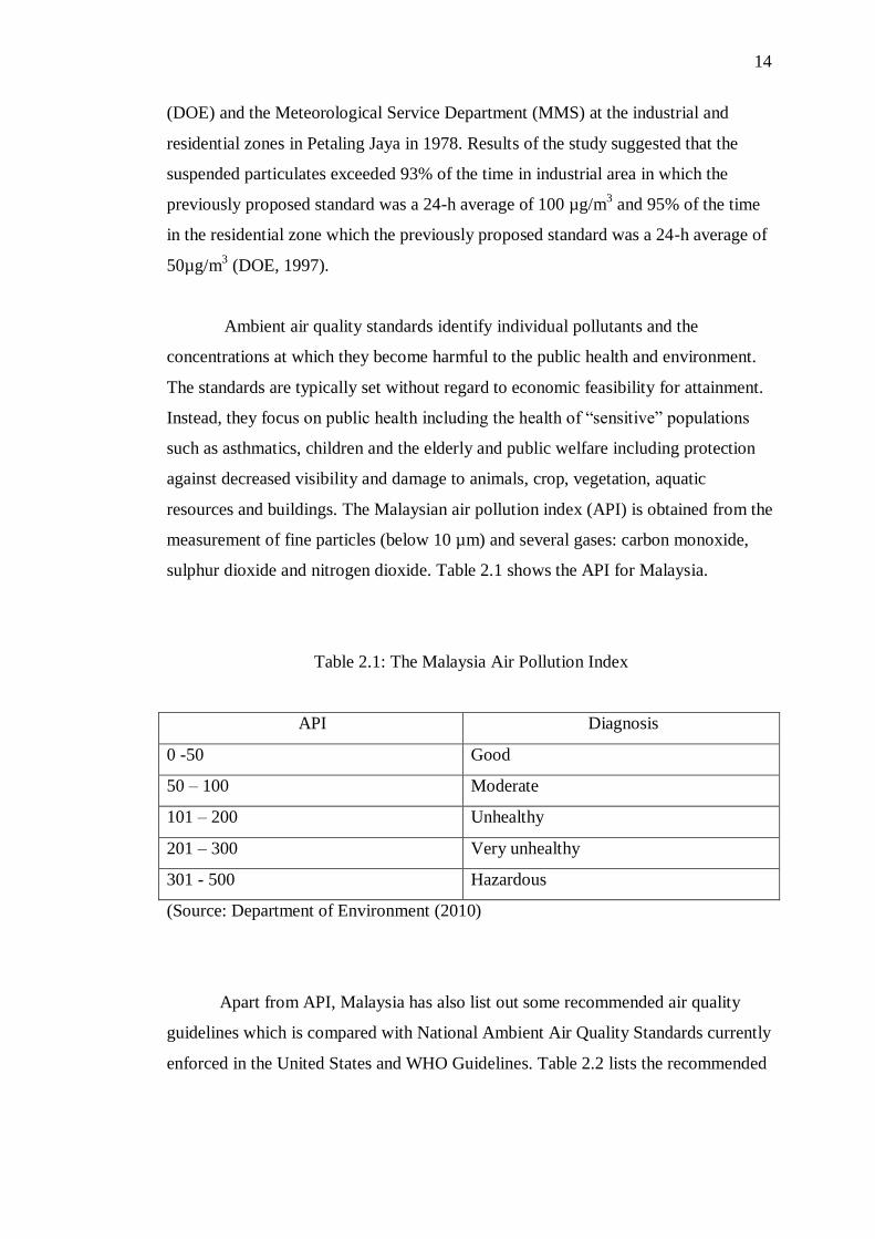
Ambient air quality standards identify individual pollutants and the

concentrations at which they become harmful to the public health and environment.

The standards are typically set without regard to economic feasibility for attainment.

Instead, they focus on public health including the health of “sensitive” populations

such as asthmatics, children and the elderly and public welfare including protection

against decreased visibility and damage to animals, crop, vegetation, aquatic

resources and buildings. The Malaysian air pollution index (API) is obtained from the

measurement of fine particles (below 10 µm) and several gases: carbon monoxide,

sulphur dioxide and nitrogen dioxide. Table 2.1 shows the API for Malaysia.

Table 2.1: The Malaysia Air Pollution Index

API Diagnosis

0 -50 Good

50 – 100 Moderate

101 – 200 Unhealthy

201 – 300 Very unhealthy

301 - 500 Hazardous

(Source: Department of Environment (2010)

Apart from API, Malaysia has also list out some recommended air quality

guidelines which is compared with National Ambient Air Quality Standards currently

enforced in the United States and WHO Guidelines. Table 2.2 lists the recommended

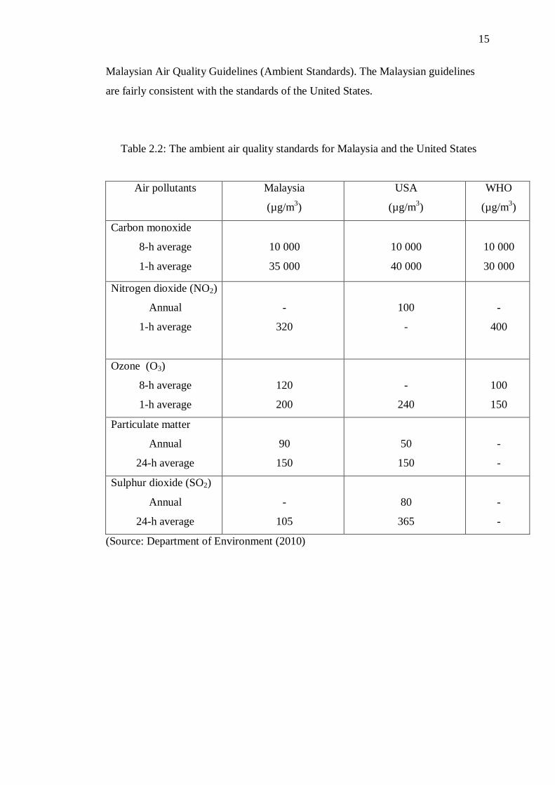
15

Malaysian Air Quality Guidelines (Ambient Standards). The Malaysian guidelines

are fairly consistent with the standards of the United States.

Table 2.2: The ambient air quality standards for Malaysia and the United States

Air pollutants Malaysia

(µg/m3)

USA

(µg/m3)

WHO

(µg/m3)

Carbon monoxide

8-h average

1-h average

10 000

35 000

10 000

40 000

10 000

30 000

Nitrogen dioxide (NO2)

Annual

1-h average

-

320

100

-

-

400

Ozone (O3)

8-h average

1-h average

120

200

-

240

100

150

Particulate matter

Annual

24-h average

90

150

50

150

-

-

Sulphur dioxide (SO2)

Annual

24-h average

-

105

80

365

-

-

(Source: Department of Environment (2010)

16

2.4 Air Pollution Studies in Malaysia

In Malaysia, few studies have been conducted on air pollution. Most of them are

related to the 1997 haze episode. In most years, the Malaysian air quality was

dominated by the occurrence of dense haze episodes. From July to October 1997,

Malaysia was badly affected by smoke haze caused by land and forest fires. Previous

incidents of severe haze in the country were reported in April 1983 (Chow and Lim,

1983), August 1990 (Cheang, 1991; Sham, 1991), June and October 1994 (Yap,

1995). The severity and extent of the 1997 smoke haze pollution were unprecedented

affecting some 300 million people across the region. The actual amount of economic

losses suffered by countries in the region during this environmental disaster were

enormous and yet to be fully determined.

During non-haze episodes, vehicular emissions accounted for more than 70%

of the total emission in the urban areas. Air quality studies conducted in the Klang

Valley during the non-haze episodes between 1986 and 1989, December 1991 to

November 1992 and January 1995 to December 1997 demonstrated two distinct daily

peaks in the diurnal variation in the concentrations of sulphur dioxide (SO2), nitrogen

dioxide (NO2), carbon monoxide and particulate matter. The morning hour peak was

mainly due to vehicle emissions and the late evening peak was attributed mainly to

meteorological conditions including atmospheric stability and wind speed. Total

suspended particulate matter was the main pollutant because the concentrations at a

few sites in the Klang Valley often exceeded the Recommended Malaysian Air

Quality Guidelines.

A comprehensive study conducted by the Department of Environment, Japan

International Cooperation Agency, the Malaysian Meteorological Service and

Universiti Putra Malaysia between December and August 1993 gave clear

indications that air pollution in the Klang Valley has become worse. This study also

indicated that if no effective counter – measures were introduced, the emissions of

sulphur oxides (SO), nitrogen oxides (NO), particulate matter, hydrocarbons and

carbon monoxides (CO) in the year 2005 would increase 1.4, 2.12, 1.47 and 2.7

times respectively to the 1992 levels (Awang et al. 1997).

17

A separate study of air quality in Kuala Lumpur found that the smoke haze

was associated with high levels of suspended microperticulate matter but with

relatively low levels of other gaseous pollutants such as carbon monoxide, nitrogen

dioxide, sulphur dioxide and ozone (Awang et al. 2000; Noor, 1998). During this

period, PM10 concentration rose beyond the Malaysian Air Quality Guidelines

(MAQG, 1989) level in almost all area monitored. It increased 4-fold higher in the

Klang Valley and up to 20-fold in Kuching (Awang et al., 2000).

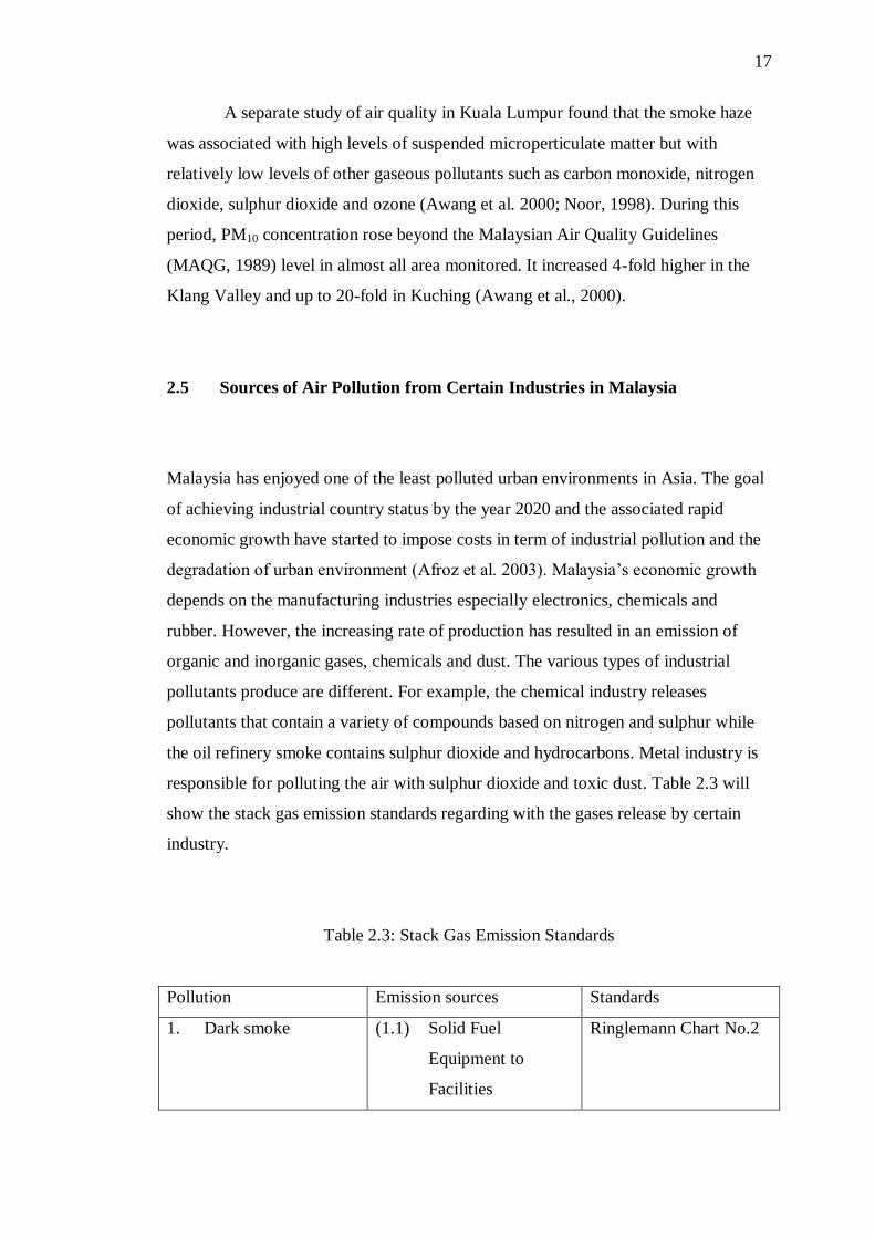
2.5 Sources of Air Pollution from Certain Industries in Malaysia

Malaysia has enjoyed one of the least polluted urban environments in Asia. The goal

of achieving industrial country status by the year 2020 and the associated rapid

economic growth have started to impose costs in term of industrial pollution and the

degradation of urban environment (Afroz et al. 2003). Malaysia‟s economic growth

depends on the manufacturing industries especially electronics, chemicals and

rubber. However, the increasing rate of production has resulted in an emission of

organic and inorganic gases, chemicals and dust. The various types of industrial

pollutants produce are different. For example, the chemical industry releases

pollutants that contain a variety of compounds based on nitrogen and sulphur while

the oil refinery smoke contains sulphur dioxide and hydrocarbons. Metal industry is

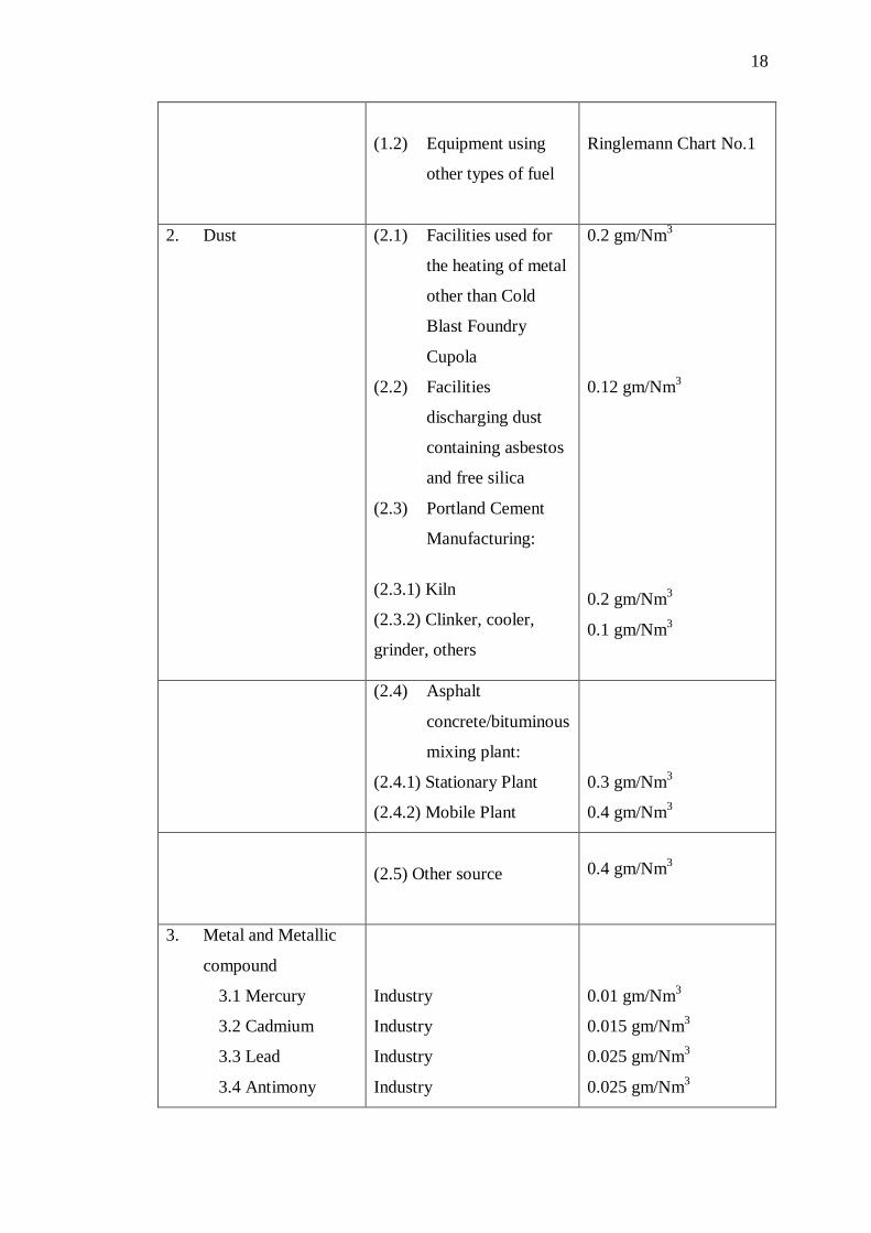
responsible for polluting the air with sulphur dioxide and toxic dust. Table 2.3 will

show the stack gas emission standards regarding with the gases release by certain

industry.

Table 2.3: Stack Gas Emission Standards

Pollution Emission sources Standards

1. Dark smoke (1.1) Solid Fuel

Equipment to

Facilities

Ringlemann Chart No.2

18

(1.2) Equipment using

other types of fuel

Ringlemann Chart No.1

2. Dust

(2.1) Facilities used for

the heating of metal

other than Cold

Blast Foundry

Cupola

(2.2) Facilities

discharging dust

containing asbestos

and free silica

(2.3) Portland Cement

Manufacturing:

(2.3.1) Kiln

(2.3.2) Clinker, cooler,

grinder, others

0.2 gm/Nm3

0.12 gm/Nm3

0.2 gm/Nm3

0.1 gm/Nm3

(2.4) Asphalt

concrete/bituminous

mixing plant:

(2.4.1) Stationary Plant

(2.4.2) Mobile Plant

0.3 gm/Nm3

0.4 gm/Nm3

(2.5) Other source

0.4 gm/Nm3

3. Metal and Metallic

compound

3.1 Mercury

3.2 Cadmium

3.3 Lead

3.4 Antimony

Industry

Industry

Industry

Industry

0.01 gm/Nm3

0.015 gm/Nm3

0.025 gm/Nm3

0.025 gm/Nm3

19

3.5 Arsenic

3.6 Zinc

3.7 Copper

Industry

Industry

Industry

0.025 gm/Nm3

0.1 gm/Nm3

0.1 gm/Nm3

4. Gases

4.1 Acid gases

4.2 Sulphuric acid

mist

4.3 Chlorine gas

4.4 HCL

4.5 Fluorine,

hydrofluoric acid,

inorganic

compound

4.6 -do -

4.7 Hydrogen

sulphide

4.8 NOx

4.9 SOx

Sulphuric Acid

manufacturing

Any sources other than

(4.1)

Any source

Any source

Aluminium manufacturing

from alumina

Any sources other than

(4.5)

Any source

Acid Nitric manufacturing

Any sources other than

(4.8)

3.5 gm of SO3/Nm3

and no persistent mist

0.2 gm of SO3/Nm3 and

no persistent mist

0.2 gm of HCl/ Nm3

0.2 gm of HCl/ Nm3

0.2 gm of Hydrofluoric

acid / Nm3

0.10 gm of Hydrofluoric

acid / Nm3

5 ppm (Vol %)

1.7 gm of SO3/Nm3 and

Substantially Colourless

2.0 gm SO3/ Nm3

(Source: Department of Environment Malaysia (2010)

Universiti Tun Hussein Onn Malaysia (UTHM) is an educational centre that

is located next to industrial area. The aforementioned industrial areas are occupied by

20

numerous industries that vary in production. There are electronic circuits, relays,

fibre boards, cardboard boxes and wood based products. All of these things produce

some sort of pollutant whether it is chemical gases release from the acid scrubber or

even some dust particulate from stack. All of the air pollutant will cross the UTHM

air space and without anybody realize, it will contribute to some sort of issues such

as haze, unwanted smell, dust particulate, sore throat or even fever.

2.6 Particulate Matter

Particulate matter is the term for solid or liquid particles found in the air. Some

particles are large or dark enough to be seen as soot or smoke. Others are so small

they can be detected only with an electron microscope. Because particles originate

from a variety of mobile and stationary sources (diesel trucks, woodstoves, power

plants, etc.), their chemical and physical compositions vary widely. Particulate

matter can be directly emitted or can be formed in the atmosphere when gaseous

pollutants such as SO2 and NOx react to form fine particles. This pollutant can cause

eye and throat irritation, and the accumulation of particulate matter in the respiratory

system is associated with numerous respiratory problems such as decreased lung

function. High levels of particulate matter can also pose health risk to sensitive

groups such as children, the elderly and individuals with asthma or cardiopulmonary

diseases. Particulate matter (PM10) can also cause undesirable impact on the

environment.

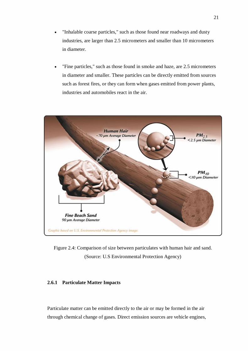
The size of particles is directly linked to their potential for causing health

problems. United States Environmental Protection Agency (USEPA) is concerned

about particles that are 10 micrometers in diameter or smaller because those are the

particles that generally pass through the throat and nose and enter the lungs. Figure

2.4 will show the comparison of size between particulates. Once inhaled, these

particles can affect the heart and lungs and cause serious health effects. USEPA

groups particle pollution into two categories:

21

"Inhalable coarse particles," such as those found near roadways and dusty

industries, are larger than 2.5 micrometers and smaller than 10 micrometers

in diameter.

"Fine particles," such as those found in smoke and haze, are 2.5 micrometers

in diameter and smaller. These particles can be directly emitted from sources

such as forest fires, or they can form when gases emitted from power plants,

industries and automobiles react in the air.

Figure 2.4: Comparison of size between particulates with human hair and sand.

(Source: U.S Environmental Protection Agency)

2.6.1 Particulate Matter Impacts

Particulate matter can be emitted directly to the air or may be formed in the air

through chemical change of gases. Direct emission sources are vehicle engines,

22

factories, construction sites, tilled fields, unpaved roads, stone crushing and burning

of wood. Indirectly formed particulate matter through reactions of gases in the

presence of water or sunlight originates from fuel combustion in motor vehicles,

power plants and other industrial processes. Particulate matter has great impacts on

human health and on the environment (Anderson et al, 2005).

2.6.1.1 Particulate Matter Impact on Humans Health

Because of its small in size, it can easily pass through our respiratory system very

easily. Some of the effects that particulate matter will bring are:

Aggravated asthma

Increase in respiratory symptoms like coughing and difficult or painful

breathing

Chronic bronchitis

Decreased lung function

Premature death.

2.6.1.2 Particulate Matter Impact on Environments

1. Visibility Impairment

Particulate matter is the major cause of reduced visibility (haze).

2. Atmospheric Deposition

Particulate matter can be carried over long distances and then settle on the ground

or in the water. Settling of Particulate matter has the following impacts:

23

acidification of lakes and rivers

change of the nutrient balance in coastal waters and large river basins

depletion of the nutrients in soil

damage of sensitive forests and farm crops

reduction of the diversity of ecosystems

3. Deterioration of Buildings and Monuments

Soot, a type of PM, stains and damages stone and other materials. This leads to

deterioration of buildings and culturally important objects such as monuments and

statues.

2.6.2 Particulate Matter Studies in Malaysia

The presence of high levels of PM10 in the atmosphere is a major cause of reduced

visibility, resulting in hazy conditions especially during the dry season. Other

environmental impacts can occur when particulate matter is deposited onto soil,

plants, water or other materials (Environmental Quality Report, 2004). Depending on

the chemical composition of these substances, when particulate matter is deposited in

sufficient quantities, it may change the nutrient balance and acidity in soil, interfere

with plant metabolism and change the composition of the materials. PM10 continues

to be the prevalent pollutant in many areas in Malaysia.

Figure 2.5 will show that the annual average levels of PM10 concentration in

the ambient air between 1996 and 2004 were just slightly below the Malaysian

Ambient Air Quality Guideline for PM10 except in 1997, when the country

experienced severe haze episodes, and in 2002, when the annual average

concentration of PM10 was equivalent to the Malaysian Ambient Air Quality

Guidelines.

24

The 1997 reading was high above the Malaysian Ambient Air Quality

Guidelines because Malaysia was one of the countries affected by 1997 Southeast

Asian haze. It was a large-scale air quality disaster which occurred during the second

half of 1997 and its after-effects causing widespread atmospheric visibility and

health problems within Southeast Asia.

Figure 2.5: Annual Average Concentration of Particulate Matter (PM10), 1996 –

2004. (Source: Environmental Quality Report, 2004)

2.7 Air Quality Dispersion Model

Air quality dispersion modelling is used to estimate concentrations of pollutants that

new (or existing) emissions sources may emit and air quality dispersion modelling is

used to predict ground level concentrations down point of sources. The object of a

model is to relate mathematically the effects of source emissions on ground level

concentrations, and to establish that permissible levels are, or are not, being

exceeded. Models have been developed to meet these objectives for a variety of

pollutants and time circumstances. Examples of emissions sources include stack

83

REFERENCES

Afroz, R., Hassan, M.N., Ibrahim, N.A., (2007). “Benefits of air quality improvement in

Klang Valley, Malaysia.” Intern J Environ Pollut 30:119 – 136.

Afroz, R., Hassan, M.N., Ibrahim, N.A., (2003). “Review of air pollution and health

impacts in Malaysia.” Environ Res 92: 71 -77.

Anderson, H.R., Atkinson, R.W., Peacock, J.L., Sweeting, M.J., Marston, L., (2005).

“Ambient Particulate Matter and Health Effects: Publication Bias in Studies of Short-

Term Associations.” Epidemiology Volume 16 - Issue 2 - pp 155-163

Awang, M.B., (1998). “Environmental studies to control the atmospheric environment in

Southeast Asia.” In: Proceedings of Asia Forum Network, Kumamoto Prefectural

Government, Japan.

Awang, M.B., Jaafar, A.B., Abdullah, A.M., Ismail, M.B., Hassan, M.N., Abdullah, R.,

Johan, S., Noor H., (2000). “Air quality in Malaysia: Impacts, management issues and

future challenges.” Respirology 5, 183 – 196.

Awang, M.B., Noor Alshrudin, S., Hassan, M.N., Abdullah, A.M., Yunos, W.M.Z.,

Haron, M.J., (1997). “Air pollution in Malaysia: Proceedings of National Conferences

on Air Pollution and Health Implications.” Centre for Enviromental Research, Institute

for Medical Research in Malaysia.

84

Azmi, S.Z., Latif, M.T., Ismail, A.S., Juneng, L., Jemain, A.A., (2009). “Trend and

status of air quality at three different monitoring stations in the Klang Valley, Malaysia.”

Air Qual Atmos Health (2010) 3: 53 - 64

Beardsley, R., Bromberg, P.A., Costa, D.A., Devlin, R., Dockery, D.W., Frampton,

M.W., Lambert, W., Samet, J.M., Speizer, F.E., Utell, M., (1997). “Smoke Alarm: Haze

From Fires Might Promote Bacterial Growth.” Sci. Am. 24 - 25.

Beychok, M.R., "Fundamentals of Stack Gas Dispersion", published by author, Irvine,

California, USA, Fourth Edition, 2005.

Brauer, M., Jamal, H.H., (1998). “Fires In Indonesia: Crisis and Reaction.” Environ. Sci.

Technol. 404 - 407.

Bosanquet, C.H., Pearson, J.L., (1936). “The Spread of Smoke and Gases from

Chimney”. Trans. Faraday Soc., 32:1249.

Cheang, (1991). Haze Episode October 1991. Malaysian Meteorological Service

Information Paper No. 2.

Chin ATH, (1996). “Containing air pollution and traffic congestion: Transport policy

and the environment in Singapore.” Atmos Environ 30: 787 – 801

Chow, K.K., Lim, J.T., (1983). “Monitoring of Suspended Particles in Petaling.” In:

Urbanization and Ecodevelopment with Special Reference to Kuala Lumpur, Institute

for Advanced Study, University of Malaya, Kuala Lumpur, pp. 178-185

Department of the Environment, Malaysia, (2004). Malaysia Environmental Quality

Report. Department of the Environment, Ministry of Science, Technology and

Environment, Malaysia.

85

Department of the Environment, Malaysia, (2001). Clean Air Regional Workshop –

Fighting Urban Air Pollution: From Plan to Action.

Department of the Environment, Malaysia, (2010). Environmental Requirements: A

Guide For Investors. Recommended Malaysian Air Quality Guidelines p.57.

Dongarrà, G., E. Manno, et al. (2010). “Study on ambient concentrations of PM10, PM10–

2.5, PM2.5 and gaseous pollutants. Trace elements and chemical speciation of atmospheric

particulates.” Atmospheric Environment 44(39): 5244-5257.

Fenger, J., (1999). “Urban Air Quality”. Atmos Environ 29:4877-4900

Godish, T., (2005). “Air Quality 4th Edition”.

Gurjar, B.R., Butler, T.M., Lawrence, M.G., Lelieveld, J., (2008). “Evaluation of Emissions

and Air Quality in Megacities.” Atmos Environ 43:1593-1606

Ilyas, S.Z., Khattak, A.I., Nasir, S.M., Qurashi, T., Durrani, R., (2009). “Air Pollution

Assessment in Urban Areas and Its Impact on Human Health in the City of Quetta,

Pakistan.” Clean Technol Environ Policy: 1-9

Mage, D., Ozolins, G., Peterson, P., Webster, A., Orthofer, R., Vandeweerd, V., Gwynne,

M., (1996). “Urban Air Pollutionin in Megacities of the World.” Atmos Environ 30:681-686

Malaysia Environmental Quality Report, (2004).

Molina, M.J., Molina, L.T., (2004). “Megacities and Atmospheric Pollution.” Air Waste

Manage Assoc 54:644-680

Nasir, M.H., Choo, W.Y., Rafia, A., Md., M.R., Theng, L.C., Noor, M.M.H., (2000).

“Estimation of Health Damage Cost For 1997 – Haze Episode in Malaysia Using Ostro

Model”. Proceeedings Malaysian Science and Technology Congress, 2000.

86

Confederation of Scientific and Technological Association in Malaysia (COST-AM),

Kuala Lumpur, in Press.

Ozden, O., Dogeroglu, T., Kara, S., (2008). “Assessment of ambient air quality in

Eskisehir, Turkey”. Environ Intern 34:678 – 687.

Pasquill, F., (1961). “The estimation of the dispersion of windborne material”. The

Meteorological Magazine, vol 90, No. 1063, pp 33-49.

Riga-Karandinos, A., Saitanis, C., (2005). “Comparative Assessment of Ambient Air

Quality in Two Typical Mediterranean Coastal Cities in Greece.” Chemosphere: 1125-

1136.

Sham, S., (1979). “Mixing Depth, Wind Speed and Air Pollution Potential in Kuala

Lumpur Petaling Jaya Area, Malaysia.” UKM Press.

Sham, S., (1991). The August 1990 Haze. In: Malaysian Meteorological Services

Technical Report. Report No. 49.

Sham, S., (1994). “Air Pollution Studies in Klang Valley, Malaysia. Some Policy

Implications.” Asian Geogr. 3, 43-50.

United States of America Environmental Protection Agency, 2011. Temperature.

United States of America Environmental Protection Agency, 2011. Topography or

Terrain Effect on Air Pollution.

United States of America Environmental Protection Agency, 2011. Particulate Matter.

United States of America Environmental Protection Agency, 2011. Wind Speed and

Wind Direction Effect on Air Pollution.

87

United States of America Strategic Plan for the Climate Change Science Program,

(2003). Final Report.

University of California Santa Barbara, (2012). Standard Atmospheric Density.

University of Michigan, (2012). Central Campus Air Quality Model (CCAQM)

Instructions

University of Leeds, United Kingdom, (2012). Atmospheric Dispersion Note for

Teaching.

World Health Organization, 2005. WHO Air Quality Guidelines for Particulate Matter,

Ozone, Nitrogen Dioxide and Sulfur Dioxide Global Update for 2005.

Yap, K.S., (1995). Haze in Malaysia. In: Meteorological Service Technical Report.