A Study on Straight-Line Tracking Bicycle

8/7/2019 A Study on Straight-Line Tracking Bicycle

http://slidepdf.com/reader/full/a-study-on-straight-line-tracking-bicycle 1/10

IEEE TRANSACTIONS ON INDUSTRIAL ELECTRONICS, VOL. 56, NO. 1, JANUARY 2009 159

A Study on Straight-Line Tracking andPosture Control in Electric Bicycle

Yasuhito Tanaka and Toshiyuki Murakami, Member, IEEE

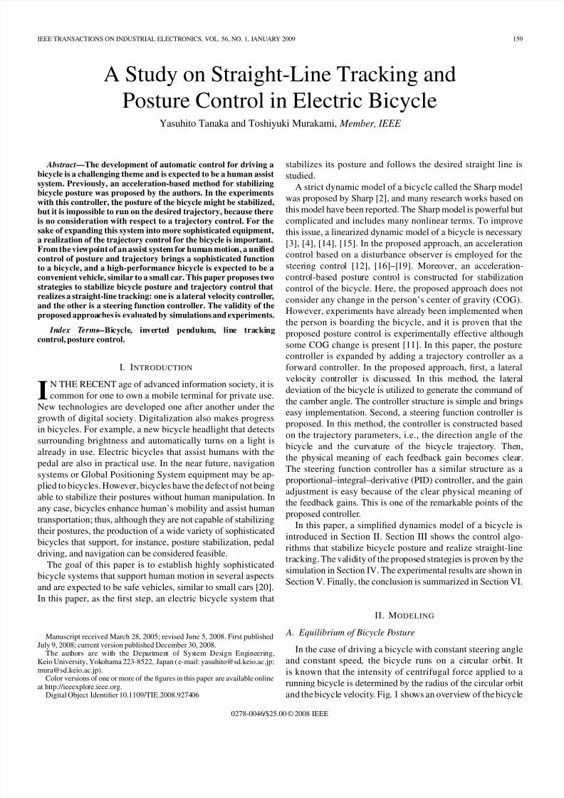
Abstract—The development of automatic control for driving abicycle is a challenging theme and is expected to be a human assistsystem. Previously, an acceleration-based method for stabilizingbicycle posture was proposed by the authors. In the experimentswith this controller, the posture of the bicycle might be stabilized,but it is impossible to run on the desired trajectory, because thereis no consideration with respect to a trajectory control. For thesake of expanding this system into more sophisticated equipment,a realization of the trajectory control for the bicycle is important.From the viewpoint of an assist system for human motion, a unifiedcontrol of posture and trajectory brings a sophisticated functionto a bicycle, and a high-performance bicycle is expected to be a

convenient vehicle, similar to a small car. This paper proposes twostrategies to stabilize bicycle posture and trajectory control thatrealizes a straight-line tracking: one is a lateral velocity controller,and the other is a steering function controller. The validity of theproposed approaches is evaluated by simulations and experiments.

Index Terms—Bicycle, inverted pendulum, line trackingcontrol, posture control.

I. INTRODUCTION

IN THE RECENT age of advanced information society, it is

common for one to own a mobile terminal for private use.

New technologies are developed one after another under the

growth of digital society. Digitalization also makes progressin bicycles. For example, a new bicycle headlight that detects

surrounding brightness and automatically turns on a light is

already in use. Electric bicycles that assist humans with the

pedal are also in practical use. In the near future, navigation

systems or Global Positioning System equipment may be ap-

plied to bicycles. However, bicycles have the defect of not being

able to stabilize their postures without human manipulation. In

any case, bicycles enhance human’s mobility and assist human

transportation; thus, although they are not capable of stabilizing

their postures, the production of a wide variety of sophisticated

bicycles that support, for instance, posture stabilization, pedal

driving, and navigation can be considered feasible.

The goal of this paper is to establish highly sophisticated

bicycle systems that support human motion in several aspects

and are expected to be safe vehicles, similar to small cars [20].

In this paper, as the first step, an electric bicycle system that

Manuscript received March 28, 2005; revised June 5, 2008. First publishedJuly 9, 2008; current version published December 30, 2008.

The authors are with the Department of System Design Engineering,Keio University, Yokohama 223-8522, Japan (e-mail: [email protected];[email protected]).

Color versions of one or more of the figures in this paper are available onlineat http://ieeexplore.ieee.org.

Digital Object Identifier 10.1109/TIE.2008.927406

stabilizes its posture and follows the desired straight line is

studied.

A strict dynamic model of a bicycle called the Sharp model

was proposed by Sharp [2], and many research works based on

this model have been reported. The Sharp model is powerful but

complicated and includes many nonlinear terms. To improve

this issue, a linearized dynamic model of a bicycle is necessary

[3], [4], [14], [15]. In the proposed approach, an acceleration

control based on a disturbance observer is employed for the

steering control [12], [16]–[19]. Moreover, an acceleration-

control-based posture control is constructed for stabilizationcontrol of the bicycle. Here, the proposed approach does not

consider any change in the person’s center of gravity (COG).

However, experiments have already been implemented when

the person is boarding the bicycle, and it is proven that the

proposed posture control is experimentally effective although

some COG change is present [11]. In this paper, the posture

controller is expanded by adding a trajectory controller as a

forward controller. In the proposed approach, first, a lateral

velocity controller is discussed. In this method, the lateral

deviation of the bicycle is utilized to generate the command of

the camber angle. The controller structure is simple and brings

easy implementation. Second, a steering function controller is

proposed. In this method, the controller is constructed basedon the trajectory parameters, i.e., the direction angle of the

bicycle and the curvature of the bicycle trajectory. Then,

the physical meaning of each feedback gain becomes clear.

The steering function controller has a similar structure as a

proportional–integral–derivative (PID) controller, and the gain

adjustment is easy because of the clear physical meaning of

the feedback gains. This is one of the remarkable points of the

proposed controller.

In this paper, a simplified dynamics model of a bicycle is

introduced in Section II. Section III shows the control algo-

rithms that stabilize bicycle posture and realize straight-line

tracking. The validity of the proposed strategies is proven by thesimulation in Section IV. The experimental results are shown in

Section V. Finally, the conclusion is summarized in Section VI.

II. MODELING

A. Equilibrium of Bicycle Posture

In the case of driving a bicycle with constant steering angle

and constant speed, the bicycle runs on a circular orbit. It

is known that the intensity of centrifugal force applied to a

running bicycle is determined by the radius of the circular orbit

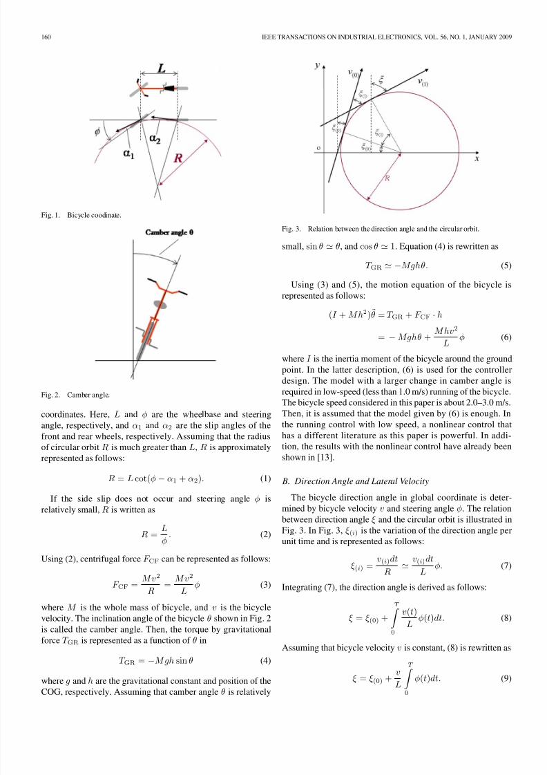
and the bicycle velocity. Fig. 1 shows an overview of the bicycle

0278-0046/$25.00 © 2008 IEEE



160 IEEE TRANSACTIONS ON INDUSTRIAL ELECTRONICS, VOL. 56, NO. 1, JANUARY 2009

Fig. 1. Bicycle coodinate.

Fig. 2. Camber angle.

coordinates. Here, L and φ are the wheelbase and steering

angle, respectively, and α1 and α2 are the slip angles of the

front and rear wheels, respectively. Assuming that the radius

of circular orbit R is much greater than L, R is approximately

represented as follows:

R = L cot(φ − α1 + α2). (1)

If the side slip does not occur and steering angle φ is

relatively small, R is written as

R =L

φ

. (2)

Using (2), centrifugal force F CF can be represented as follows:

F CF =Mv2

R=

Mv2

Lφ (3)

where M is the whole mass of bicycle, and v is the bicycle

velocity. The inclination angle of the bicycle θ shown in Fig. 2

is called the camber angle. Then, the torque by gravitational

force T GR is represented as a function of θ in

T GR = −M gh sin θ (4)

where g and h are the gravitational constant and position of theCOG, respectively. Assuming that camber angle θ is relatively

Fig. 3. Relation between the direction angle and the circular orbit.

small, sin θ θ, and cos θ 1. Equation (4) is rewritten as

T GR −Mghθ. (5)

Using (3) and (5), the motion equation of the bicycle is


(I + M h2)θ = T GR + F CF · h

= − Mghθ +M hv2

Lφ (6)

where I is the inertia moment of the bicycle around the ground

point. In the latter description, (6) is used for the controller

design. The model with a larger change in camber angle is

required in low-speed (less than 1.0 m/s) running of the bicycle.

The bicycle speed considered in this paper is about 2.0–3.0 m/s.

Then, it is assumed that the model given by (6) is enough. In

the running control with low speed, a nonlinear control that

has a different literature as this paper is powerful. In addi-

tion, the results with the nonlinear control have already been

shown in [13].

B. Direction Angle and Lateral Velocity

The bicycle direction angle in global coordinate is deter-

mined by bicycle velocity v and steering angle φ. The relation

between direction angle ξ and the circular orbit is illustrated in

Fig. 3. In Fig. 3, ξ(i) is the variation of the direction angle per

unit time and is represented as follows:

ξ(i) =v(i)dt

R

v(i)dt

Lφ. (7)

Integrating (7), the direction angle is derived as follows:

ξ = ξ(0) +

T

0

v(t)

Lφ(t)dt. (8)

Assuming that bicycle velocity v is constant, (8) is rewritten as

ξ = ξ(0) +v

L

T

0

φ(t)dt. (9)



TANAKA AND MURAKAMI: STUDY ON STRAIGHT-LINE TRACKING AND POSTURE CONTROL IN ELECTRIC BICYCLE 161

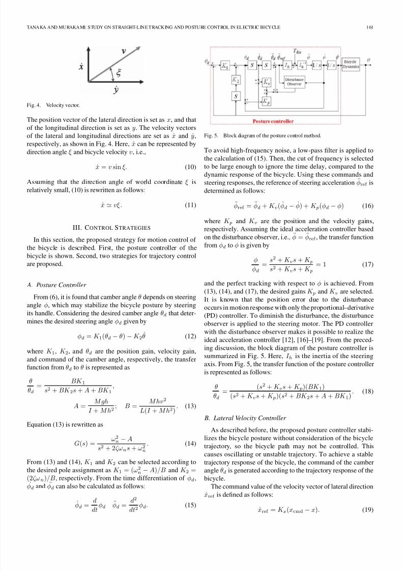
Fig. 4. Velocity vector.

The position vector of the lateral direction is set as x, and that

of the longitudinal direction is set as y. The velocity vectors

of the lateral and longitudinal directions are set as x and y,

respectively, as shown in Fig. 4. Here, x can be represented by

direction angle ξ and bicycle velocity v, i.e.,

x = v sin ξ. (10)

Assuming that the direction angle of world coordinate ξ is

relatively small, (10) is rewritten as follows:

x vξ. (11)

III. CONTROL STRATEGIES

In this section, the proposed strategy for motion control of

the bicycle is described. First, the posture controller of the

bicycle is shown. Second, two strategies for trajectory control

are proposed.

A. Posture Controller

From (6), it is found that camber angle θ depends on steeringangle φ, which may stabilize the bicycle posture by steering

its handle. Considering the desired camber angle θd that deter-

mines the desired steering angle φd given by

φd = K 1(θd − θ) − K 2θ (12)

where K 1, K 2, and θd are the position gain, velocity gain,

and command of the camber angle, respectively, the transfer

function from θd to θ is represented as

θ

θd=

BK 1s2 + BK 2s + A + BK 1

,

A = M ghI + M h2

; B = M hv2

L(I + M h2). (13)

Equation (13) is rewritten as

G(s) =ω2n − A

s2 + 2ζωns + ω2n

. (14)

From (13) and (14), K 1 and K 2 can be selected according to

the desired pole assignment as K 1 = (ω2n − A)/B and K 2 =

(2ζωn)/B, respectively. From the time differentiation of φd,

φd and φd can also be calculated as follows:

φd = ddt

φd φd = d2dt2

φd. (15)

Fig. 5. Block diagram of the posture control method.

To avoid high-frequency noise, a low-pass filter is applied to

the calculation of (15). Then, the cut of frequency is selected

to be large enough to ignore the time delay, compared to the

dynamic response of the bicycle. Using these commands and

steering responses, the reference of steering acceleration φref is

determined as follows:

φref = φd + K v(φd − φ) + K p(φd − φ) (16)

where K p and K v are the position and the velocity gains,

respectively. Assuming the ideal acceleration controller based

on the disturbance observer, i.e., φ = φref , the transfer function

from φd to φ is given by

φ

φd

=s2 + K vs + K ps2 + K vs + K p

= 1 (17)

and the perfect tracking with respect to φ is achieved. From

(13), (14), and (17), the desired gains K p and K v are selected.

It is known that the position error due to the disturbanceoccurs in motion response with only the proportional–derivative

(PD) controller. To diminish the disturbance, the disturbance

observer is applied to the steering motor. The PD controller

with the disturbance observer makes it possible to realize the

ideal acceleration controller [12], [16]–[19]. From the preced-

ing discussion, the block diagram of the posture controller is

summarized in Fig. 5. Here, I h is the inertia of the steering

axis. From Fig. 5, the transfer function of the posture controller

is represented as follows:

θ

θd=

(s2 + K vs + K p)(BK 1)

(s2 + K vs + K p)(s2 + BK 2s + A + BK 1). (18)

B. Lateral Velocity Controller

As described before, the proposed posture controller stabi-

lizes the bicycle posture without consideration of the bicycle

trajectory, so the bicycle path may not be controlled. This

causes oscillating or unstable trajectory. To achieve a stable

trajectory response of the bicycle, the command of the camber

angle θd is generated according to the trajectory response of the

bicycle.

The command value of the velocity vector of lateral direction

xref is defined as follows:

xref = K x(xcmd − x). (19)




Here, K x is the proportional gain, and xcmd is the position

command of the target trajectory. By using (11) and (19), the

command of the direction angle ξcmd is determined as follows:

xref = vξcmd

ξcmd =

xref

v =

K x(xcmd − x)

v . (20)

In the case that the centrifugal force equilibrates with the

effect of gravity, the acceleration of the bicycle inclination θbecomes zero, i.e., θ = 0. The acceleration response of the

camber angle has little effect on the posture controller, even

if it is not assumed to be zero. However, it is necessary to

consider it to improve the transient state of the camber angle.

The improvement of transient state is one of the future works

although the posture controller is stable. The steering angle φin equilibrium state is derived from (6) as follows:

−Mghθ + Mhv2

L φ = 0, φ =gL

v2 θ; θ =v2

gL φ. (21)

Substituting (21) into (9),

ξ = ξ(0) +v

L

T

0

φ(t)dt

= ξ(0) +g

v

T

0

θ(t)dt (22)

is derived. From (22), the following equations are obtained:

ξcmd = ξcmd(0) +g

v

T

0

θd(t)dt

ξcmd =g

vθd

θd =v

gξcmd. (23)

Differentiating (20) with respect to time t and substituting it to

(23), the command of the camber angle θd is derived as follows:

ξcmd = xref v

= K x(xcmd − x)v

θd =v

gξcmd

=v

g·

K x(xcmd − x)

v. (24)

Assuming that a bicycle posture is stable like a four-wheel car

[21], [22], the transfer function from the position command in

lateral direction xcmd to the position of lateral direction x is


xxcmd

= BK 1K x(s2 + K 1Bs + A + BK 1)(s + K x)

. (25)

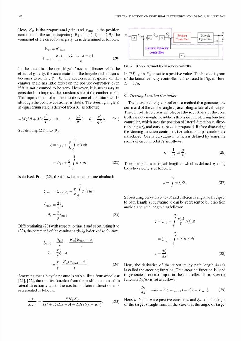
Fig. 6. Block diagram of lateral velocity controller.

In (25), gain K x is set to a positive value. The block diagram

of the lateral velocity controller is illustrated in Fig. 6. Here,

D = 1/g.

C. Steering Function Controller

The lateral velocity controller is a method that generates the

command of the camber angle θd according to lateral velocity x.

The control structure is simple, but the robustness of the con-

troller is not enough. To address this issue, the steering function

controller, which uses the position of lateral direction x, direc-

tion angle ξ, and curvature κ, is proposed. Before discussing

the steering function controller, two additional parameters are

introduced. One is curvature κ, which is defined by using the

radius of circular orbit R as follows:

κ =1

R

φ

L. (26)

The other parameter is path length s, which is defined by using

bicycle velocity v as follows:

s =

T 0

v(t)dt. (27)

Substituting curvature κ to (8) and differentiating it with respect

to path length s, curvature κ can be represented by direction

angle ξ and path length s as follows:

ξ = ξ(0) +

T

0

v(t)

Lφ(t)dt

= ξ(0) +

T

0

v(t)κ(t)dt

κ =dξ

ds. (28)

Here, the derivative of the curvature by path length dκ/dsis called the steering function. This steering function is used

to generate a control input in the controller. Then, steering

function dκ/ds is set as follows:

dκ

ds= −aκ − b(ξ − ξcmd) − c(x − xcmd). (29)

Here, a, b, and c are positive constants, and ξcmd is the angleof the target straight line. In the case that the angle of target




straight line ξcmd and xcmd are zero, steering function dκ/dsbecomes

dκ

ds= −aκ − bξ − cx. (30)

To select appropriate gains of positive constants a, b, and c, (30)

is rewritten as a first-order equation of the system. Here, bicycledirection angle ξ is geometrically represented as follows:

ξ = tan−1 dx

dy. (31)

In the case that the bicycle follows a straight line, the moving

distance of the longitudinal direction becomes much longer

than that of the lateral direction, and bicycle direction angle ξis approximated as follows:

ξ = tan−1 dx

dy

dx

dy. (32)

Similarly, the derivative of path length s is approximated by the

moving distance of the longitudinal direction y. Curvature κand steering function dκ/ds are represented by the derivative of

the moving distance of the longitudinal direction y as follows:

κ =dξ

ds

dξ

dy(33)

dκ

ds= − aκ − bξ − cx

dκ

dy. (34)

From (32)–(34), the first-order equation of the system is de-

rived as

X =

⎡⎣ 0 1 0

0 0 1−c −b −a

⎤⎦X = AX

A ≡

⎡⎣ 0 1 0

0 0 1−c −b −a

⎤⎦X ≡

⎡⎣x(y)

ξ(y)κ(y)

⎤⎦ . (35)

Here, indicates the derivative of the moving distance of the

longitudinal direction y. The characteristic equation of A is

given as follows:

det[λI −A] = λ3 + aλ2 + bλ + c = 0. (36)

To obtain the condition of asymptotic stability, the eigenvalues

λ in (36) must be negative numbers. Assuming that (36) is

rewritten as

(λ + k)3 = 0, k > 0. (37)

eigenvalues λ are selected as negative numbers. Parameter k is

a positive real number. By using k, a, b, and c can easily be

obtained, i.e.,

(λ + k)3 = λ3 + 3kλ2 + 3k2λ + k3

= λ3 + aλ2 + bλ + c

= 0,a = 3k; b = 3k2; c = k3. (38)

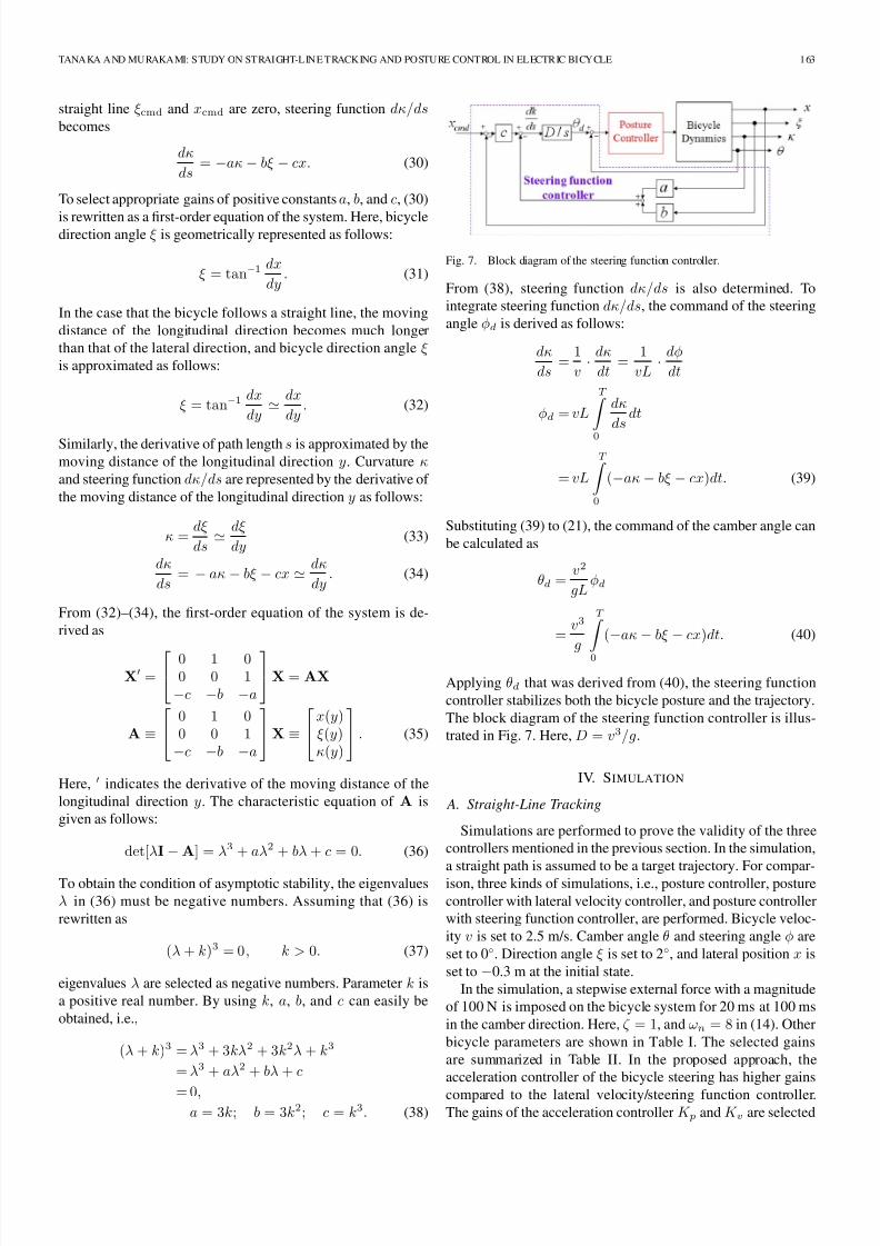
Fig. 7. Block diagram of the steering function controller.

From (38), steering function dκ/ds is also determined. To

integrate steering function dκ/ds, the command of the steering

angle φd is derived as follows:

dκ

ds=

1

v·

dκ

dt=

1

vL·

dφ

dt

φd = vL

T

0

dκ

dsdt

= vL

T

0

(−aκ − bξ − cx)dt. (39)

Substituting (39) to (21), the command of the camber angle can

be calculated as

θd =v2

gLφd

=v3

g

T

0

(−aκ − bξ − cx)dt. (40)

Applying θd that was derived from (40), the steering function

controller stabilizes both the bicycle posture and the trajectory.

The block diagram of the steering function controller is illus-

trated in Fig. 7. Here, D = v3/g.

IV. SIMULATION

A. Straight-Line Tracking

Simulations are performed to prove the validity of the three

controllers mentioned in the previous section. In the simulation,

a straight path is assumed to be a target trajectory. For compar-ison, three kinds of simulations, i.e., posture controller, posture

controller with lateral velocity controller, and posture controller

with steering function controller, are performed. Bicycle veloc-

ity v is set to 2.5 m/s. Camber angle θ and steering angle φ are

set to 0◦. Direction angle ξ is set to 2◦, and lateral position x is

set to −0.3 m at the initial state.

In the simulation, a stepwise external force with a magnitude

of 100 N is imposed on the bicycle system for 20 ms at 100 ms

in the camber direction. Here, ζ = 1, and ωn = 8 in (14). Other

bicycle parameters are shown in Table I. The selected gains

are summarized in Table II. In the proposed approach, the

acceleration controller of the bicycle steering has higher gains

compared to the lateral velocity/steering function controller.The gains of the acceleration controller K p and K v are selected




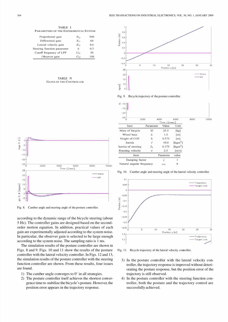
TABLE IPARAMETERS OF THE EXPERIMENTAL SYSTEM

TABLE IIGAINS OF THE CONTROLLER

Fig. 8. Camber angle and steering angle of the posture controller.

according to the dynamic range of the bicycle steering (about

5 Hz). The controller gains are designed based on the second-

order motion equation. In addition, practical values of each

gain are experimentally adjusted according to the system noise.

In particular, the observer gain is selected to be large enough

according to the system noise. The sampling ratio is 1 ms.

The simulation results of the posture controller are shown in

Figs. 8 and 9. Figs. 10 and 11 show the results of the posture

controller with the lateral velocity controller. In Figs. 12 and 13,

the simulation results of the posture controller with the steering

function controller are shown. From these results, four issues

are found.

1) The camber angle converges to 0◦ in all strategies.

2) The posture controller itself achieves the shortest conver-

gence time to stabilize the bicycle’s posture. However, theposition error appears in the trajectory response.

Fig. 9. Bicycle trajectory of the posture controller.

Fig. 10. Camber angle and steering angle of the lateral velocity controller.

Fig. 11. Bicycle trajectory of the lateral velocity controller.

3) In the posture controller with the lateral velocity con-

troller, the trajectory response is improved without deteri-

orating the posture response, but the position error of the

trajectory is still observed.

4) In the posture controller with the steering function con-

troller, both the posture and the trajectory control aresuccessfully achieved.




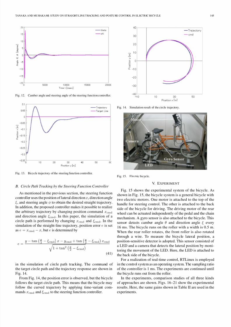
Fig. 12. Camber angle and steering angle of the steering function controller.

Fig. 13. Bicycle trajectory of the steering function controller.

B. Circle Path Tracking by the Steering Function Controller

As mentioned in the previous section, the steering function

controller uses the position of lateral direction x, direction angle

ξ, and steering angle φ to obtain the desired straight trajectory.

In addition, the proposed controller makes it possible to realize

the arbitrary trajectory by changing position command xcmd

and direction angle ξcmd. In this paper, the simulation of a

circle path is performed by changing xcmd and ξcmd. In the

simulation of the straight-line trajectory, position error e is set

as e = xcmd − x, but e is determined by

e =y − tan

π2 − ξcmd

x − ycmd + tan

π2 − ξcmd

xcmd

1 + tan2π2 − ξcmd

(41)

in the simulation of circle path tracking. The command of

the target circle path and the trajectory response are shown in

Fig. 14.

From Fig. 14, the position error is observed, but the bicycle

follows the target circle path. This means that the bicycle may

follow the curved trajectory by applying time-variant com-mands xcmd and ξcmd to the steering function controller.

Fig. 14. Simulation result of the circle trajectory.

Fig. 15. Electric bicycle.

V. EXPERIMENT

Fig. 15 shows the experimental system of the bicycle. As

shown in Fig. 15, the bicycle system is a general bicycle with

two electric motors. One motor is attached to the top of the

handle for steering control. The other is attached to the back

side of the bicycle for driving. The driving motor of the rear

wheel can be actuated independently of the pedal and the chain

mechanism. A gyro sensor is also attached to the bicycle. This

sensor detects camber angle θ and direction angle ξ every

16 ms. The bicycle runs on the roller with a width is 0.5 m.When the rear roller rotates, the front roller is also rotated

through a wire. To measure the bicycle lateral position, a

position-sensitive detector is adopted. This sensor consisted of

a LED and a camera that detects the lateral position by moni-

toring the movement of the LED. Here, the LED is attached to

the back side of the bicycle.

For a realization of real-time control, RTLinux is employed

in the control system as an operating system. The sampling ratio

of the controller is 1 ms. The experiments are continued until

the bicycle runs out from the roller.

In the experiments, comparison studies of all three kinds

of approaches are shown. Figs. 16–21 show the experimental

results. Here, the same gains shown in Table II are used in theexperiments.




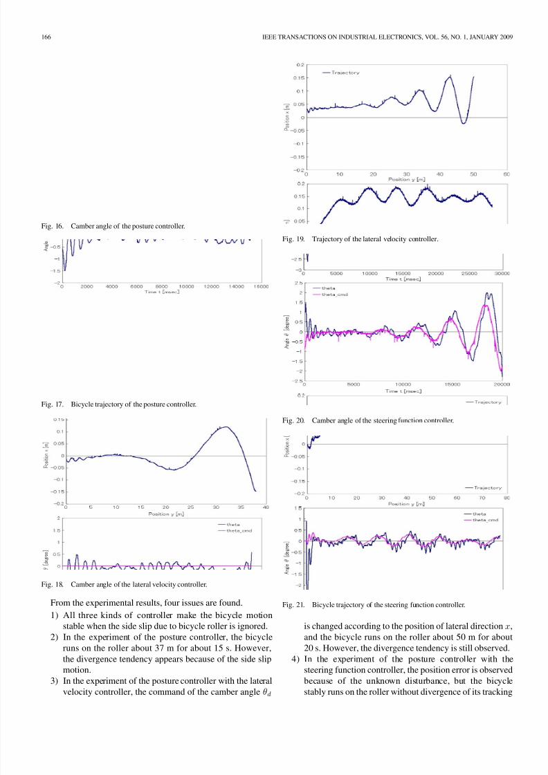
Fig. 16. Camber angle of the posture controller.

Fig. 17. Bicycle trajectory of the posture controller.

Fig. 18. Camber angle of the lateral velocity controller.

From the experimental results, four issues are found.

1) All three kinds of controller make the bicycle motion

stable when the side slip due to bicycle roller is ignored.

2) In the experiment of the posture controller, the bicycle

runs on the roller about 37 m for about 15 s. However,

the divergence tendency appears because of the side slip

motion.

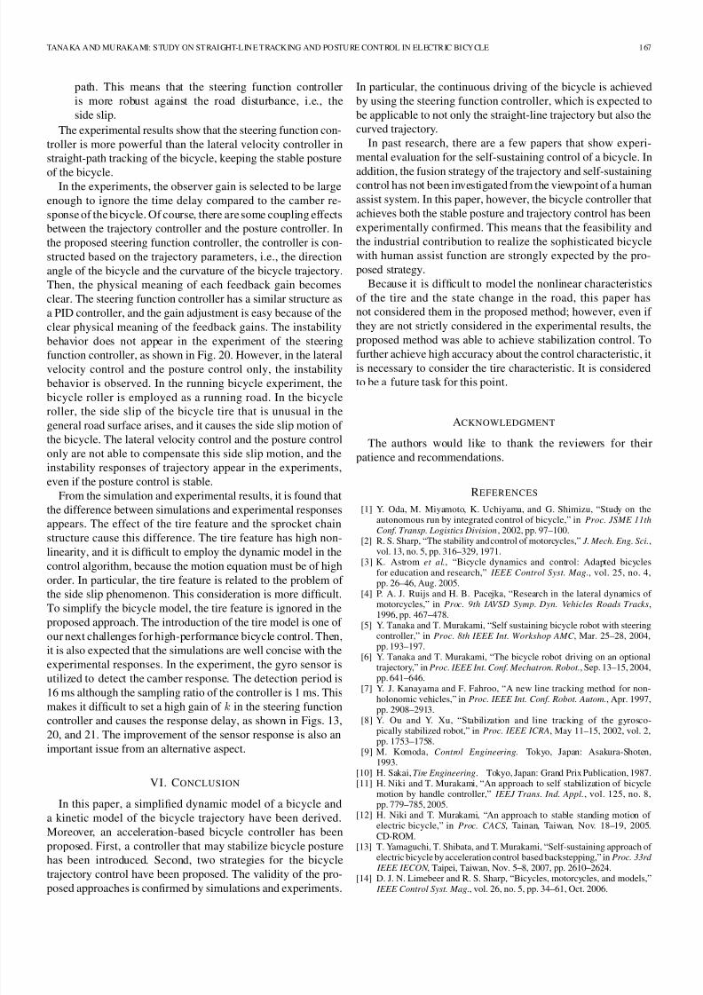
3) In the experiment of the posture controller with the lateralvelocity controller, the command of the camber angle θd

Fig. 19. Trajectory of the lateral velocity controller.

Fig. 20. Camber angle of the steering function controller.

Fig. 21. Bicycle trajectory of the steering function controller.

is changed according to the position of lateral direction x,

and the bicycle runs on the roller about 50 m for about

20 s. However, the divergence tendency is still observed.

4) In the experiment of the posture controller with the

steering function controller, the position error is observed

because of the unknown disturbance, but the bicyclestably runs on the roller without divergence of its tracking




path. This means that the steering function controller

is more robust against the road disturbance, i.e., the

side slip.

The experimental results show that the steering function con-

troller is more powerful than the lateral velocity controller in

straight-path tracking of the bicycle, keeping the stable posture

of the bicycle.In the experiments, the observer gain is selected to be large

enough to ignore the time delay compared to the camber re-

sponse of the bicycle. Of course, there are some coupling effects

between the trajectory controller and the posture controller. In

the proposed steering function controller, the controller is con-

structed based on the trajectory parameters, i.e., the direction

angle of the bicycle and the curvature of the bicycle trajectory.

Then, the physical meaning of each feedback gain becomes

clear. The steering function controller has a similar structure as

a PID controller, and the gain adjustment is easy because of the

clear physical meaning of the feedback gains. The instability

behavior does not appear in the experiment of the steering

function controller, as shown in Fig. 20. However, in the lateral

velocity control and the posture control only, the instability

behavior is observed. In the running bicycle experiment, the

bicycle roller is employed as a running road. In the bicycle

roller, the side slip of the bicycle tire that is unusual in the

general road surface arises, and it causes the side slip motion of

the bicycle. The lateral velocity control and the posture control

only are not able to compensate this side slip motion, and the

instability responses of trajectory appear in the experiments,

even if the posture control is stable.

From the simulation and experimental results, it is found that

the difference between simulations and experimental responses

appears. The effect of the tire feature and the sprocket chainstructure cause this difference. The tire feature has high non-

linearity, and it is difficult to employ the dynamic model in the

control algorithm, because the motion equation must be of high

order. In particular, the tire feature is related to the problem of

the side slip phenomenon. This consideration is more difficult.

To simplify the bicycle model, the tire feature is ignored in the

proposed approach. The introduction of the tire model is one of

our next challenges for high-performance bicycle control. Then,

it is also expected that the simulations are well concise with the

experimental responses. In the experiment, the gyro sensor is

utilized to detect the camber response. The detection period is

16 ms although the sampling ratio of the controller is 1 ms. Thismakes it difficult to set a high gain of k in the steering function

controller and causes the response delay, as shown in Figs. 13,

20, and 21. The improvement of the sensor response is also an

important issue from an alternative aspect.

VI. CONCLUSION

In this paper, a simplified dynamic model of a bicycle and

a kinetic model of the bicycle trajectory have been derived.

Moreover, an acceleration-based bicycle controller has been

proposed. First, a controller that may stabilize bicycle posture

has been introduced. Second, two strategies for the bicycle

trajectory control have been proposed. The validity of the pro-posed approaches is confirmed by simulations and experiments.

In particular, the continuous driving of the bicycle is achieved

by using the steering function controller, which is expected to

be applicable to not only the straight-line trajectory but also the

curved trajectory.

In past research, there are a few papers that show experi-

mental evaluation for the self-sustaining control of a bicycle. In

addition, the fusion strategy of the trajectory and self-sustainingcontrol has not been investigated from the viewpoint of a human

assist system. In this paper, however, the bicycle controller that

achieves both the stable posture and trajectory control has been

experimentally confirmed. This means that the feasibility and

the industrial contribution to realize the sophisticated bicycle

with human assist function are strongly expected by the pro-

posed strategy.

Because it is difficult to model the nonlinear characteristics

of the tire and the state change in the road, this paper has

not considered them in the proposed method; however, even if

they are not strictly considered in the experimental results, the

proposed method was able to achieve stabilization control. To

further achieve high accuracy about the control characteristic, it

is necessary to consider the tire characteristic. It is considered

to be a future task for this point.

ACKNOWLEDGMENT

The authors would like to thank the reviewers for their

patience and recommendations.

REFERENCES

[1] Y. Oda, M. Miyamoto, K. Uchiyama, and G. Shimizu, “Study on the

autonomous run by integrated control of bicycle,” in Proc. JSME 11thConf. Transp. Logistics Division, 2002, pp. 97–100.[2] R. S. Sharp, “The stability and control of motorcycles,” J. Mech. Eng. Sci.,

vol. 13, no. 5, pp. 316–329, 1971.[3] K. Astrom et al., “Bicycle dynamics and control: Adapted bicycles

for education and research,” IEEE Control Syst. Mag., vol. 25, no. 4,pp. 26–46, Aug. 2005.

[4] P. A. J. Ruijs and H. B. Pacejka, “Research in the lateral dynamics of motorcycles,” in Proc. 9th IAVSD Symp. Dyn. Vehicles Roads Tracks,1996, pp. 467–478.

[5] Y. Tanaka and T. Murakami, “Self sustaining bicycle robot with steeringcontroller,” in Proc. 8th IEEE Int. Workshop AMC , Mar. 25–28, 2004,pp. 193–197.

[6] Y. Tanaka and T. Murakami, “The bicycle robot driving on an optionaltrajectory,” in Proc. IEEE Int. Conf. Mechatron. Robot., Sep. 13–15, 2004,pp. 641–646.

[7] Y. J. Kanayama and F. Fahroo, “A new line tracking method for non-

holonomic vehicles,” in Proc. IEEE Int. Conf. Robot. Autom., Apr. 1997,pp. 2908–2913.

[8] Y. Ou and Y. Xu, “Stabilization and line tracking of the gyrosco-pically stabilized robot,” in Proc. IEEE ICRA, May 11–15, 2002, vol. 2,pp. 1753–1758.

[9] M. Komoda, Control Engineering. Tokyo, Japan: Asakura-Shoten,1993.

[10] H. Sakai, Tire Engineering. Tokyo, Japan: Grand Prix Publication, 1987.[11] H. Niki and T. Murakami, “An approach to self stabilization of bicycle

motion by handle controller,” IEEJ Trans. Ind. Appl., vol. 125, no. 8,pp. 779–785, 2005.

[12] H. Niki and T. Murakami, “An approach to stable standing motion of electric bicycle,” in Proc. CACS, Tainan, Taiwan, Nov. 18–19, 2005.CD-ROM.

[13] T. Yamaguchi, T. Shibata, and T. Murakami, “Self-sustaining approach of electric bicycle by acceleration control based backstepping,” in Proc. 33rd

IEEE IECON , Taipei, Taiwan, Nov. 5–8, 2007, pp. 2610–2624.[14] D. J. N. Limebeer and R. S. Sharp, “Bicycles, motorcycles, and models,” IEEE Control Syst. Mag., vol. 26, no. 5, pp. 34–61, Oct. 2006.




[15] A. L. Schwab, J. P. Meijaard, and J. M. Papadopoulos, “A multibody dy-namics benchmarkon the equations of motion of an uncontrolled bicycle,”in Proc. 5th EUROMECH Nonlinear Dyn. Conf., 2005, pp. 511–521.

[16] K. Ohnishi, M. Shibata, and T. Murakami, “Motion control for advancedmechatronics,” IEEE/ASME Trans. Mechatronics, vol. 1, no. 1, pp. 56–67,Mar. 1996.

[17] T. Murakami, F. Yu, and K. Ohnishi, “Torque sensorless control inmultidegree-of-freedom manipulator,” IEEE Trans. Ind. Electron., vol. 40,

no. 2, pp. 259–265, Apr. 1993.[18] T. Murakami, N. Oda, Y. Miyazawa, and K. Ohnishi, “A motion con-trol strategy based on equivalent mass matrix in multidegree-of-freedommanipulator,” IEEE Trans. Ind. Electron., vol. 42, no. 2, pp. 123–130,Apr. 1995.

[19] K. Matsushita and T. Murakami, “Nonholonomic equivalent disturbancebased backward motion control of tractor-trailer with virtual steering,”

IEEE Trans. Ind. Electron., vol. 55, no. 1, pp. 280–287, Jan. 2008.[20] H. Takahashi, D. Ukishima, K. Kawamoto, and K. Hirota, “A study on

predicting hazard factors for safe driving,” IEEE Trans. Ind. Electron.,vol. 54, no. 2, pp. 781–789, Apr. 2007.

[21] N. Mutoh, T. Kazama, and K. Takita, “Driving characteristics of anelectric vehicle system with independently driven front and rear wheels,”

IEEE Trans. Ind. Electron., vol. 53, no. 3, pp. 803–813, Jun. 2006.[22] N. Mutoh, Y. Hayano, H. Yahagi, and K. Takita, “Electric braking con-

trol methods for electric vehicles with independently driven front andrear wheels,” IEEE Trans. Ind. Electron., vol. 54, no. 2, pp. 1168–1176,

Apr. 2007.

Yasuhito Tanaka received the B.E. and M.E. de-grees from Keio University, Yokohama, Japan, in2003 and 2005, respectively.

He is currently with the Department of SystemDesign Engineering, Keio University. His researchinterests include robotics, intelligent bicycles, andmotion control.

Toshiyuki Murakami (M’93) received the B.E.,M.E., and Ph.D. degrees in electrical engineeringfrom Keio University, Yokohama, Japan, in 1988,1990, and 1993, respectively.

In 1993, he joined the Department of ElectricalEngineering, Keio University, where he is currentlya Professor with the Department of System DesignEngineering. From 1999 to 2000, he was a VisitingResearcher with The Institute for Power Electronicsand Electrical Drives, Aachen University of Tech-nology, Aachen, Germany. His research interests in-

clude robotics, intelligent vehicles, mobile robots, and motion control.

A Study on Straight-Line Tracking Bicycle

Documents

Transcript of A Study on Straight-Line Tracking Bicycle