A study of wave forces on an offshore platform by direct CFDand Morison equation

D. Zhang1,a and E. G. Paterson1,b

1Virginia Polytechnic Institute and State University, Blacksburg, Virginia, 24060, USA

Abstract. Engineering simulation tools for hydrodynamic loads on offshore platforms

(e.g. NREL’s HydroDyn and Orcina’s OrcaFlex) use simplified theories and empirical

models. The most common is the Morison’s equation which accounts for unsteady drag

and inertial forces created by incident waves. Coefficients are required for these models

and are typically derived from wave-tank or pulsatile U-Shaped water tunnel experiments.

The first step of this study focuses on the application of Morison’s equations for

computing forces on a 3D platform using both computational fluid dynamics computed

and empirical coefficients. Wave forces on a simple structure, such as a bottom–

mounted monopile, are estimated by a strip–wise application of Morison’s equation

on each section. The fluid particles orbit and kinematics at strip–wise depth are

readily derived from wave theory, and the total wave force on the supporting structure

is computed by performing a simple integration in the vertical direction over each section.

The next step is the presentation of 3D multiphase RANS simulation of the wind-turbine

platform in single-harmonic regular waves. Simulation results from full 3D simulation

will be compared to the results from Morison’s equation. We are motivated by the chal-

lenges of a floating platform which has complex underwater geometry (e.g. tethered

semi-submersible). In cases like this, our hypothesis is that Morison’s equation will re-

sult in inaccurate prediction of forces, due to the limitations of 2D coefficients of simple

geometries, and that 3D multiphase RANS CFD will be required to generate reliable

predictions of platform loads and motions.

1 Introduction

1.1 Motivation

Cyber Wind Facility (CWF) is a computational facility designed to generate data that cannot be col-

lected from a field wind turbine facility, which has limited data collection capabilities (Brasseur et al.,

2013). By using petascale computer systems, CWF can generate four-dimensional data over the en-

tire domain in a controlled cyber environment, specifically including highly resolved 4-D cyber data;

ae-mail: liybzd@vt.edube-mail: egp@vt.edu

DOI: 10.1051/C© Owned by the authors, published by EDP Sciences, 2015

/

0 0 ( 2015)201

Web of Conferences ,5 0 0

00

5E S3e sconf3 05

44

��������������� �������� ��������������������������������������������������������������������� ������������� ���������

�������� ��������������������������������� ����������������������������������� ��������!����������� ������

22

Article available at http://www.e3s-conferences.org or http://dx.doi.org/10.1051/e3sconf/20150504002

coupled wind-loading-torque data; coupled wave-motion-loadings data; test-bed, design and controls

concepts and correlations for advanced design tools.

As a vital part of the whole project, the hydrodynamics module solves the 6-DOF equations of the

tower-rotor-platform by applying hybrid URANS-LES around the platform coupled to a wave model

with wide variety of wave characteristics. The resulting data can be used both in the design stage and

performance calculation.

Current state-of-art engineering tools, for example NREL’s Hydrodyn, OrcaFlex and ANSYS

AQWA, are based upon semi-emperical time-domain methods, e.g., Cummins equation (Cummins,

1962). These models use various theories for radiation, diffraction, hydrostatics, and viscous effects.

Morison’s equation is commonly used for damping and inertia forces due to wave excitation.

For certain wave-structure configuration, for example the OC3 spar buoy platform (Jonkman,

2010), Morison’s equation provides reasonable accuracy of wave forces on the floating structure.

Large amount of historical data is available for simple geometries, e.g. circular cylinders. Some

floating platforms have complex underwater geometry, e.g. OC4 Semi-submersible, which precludes

the use of theoretical or historical data for drag, inertial, damping, added mass, etc.

1.2 Objective

There are two objectives of the current study:

1) RANS CFD for fixed platformThe objective of the current study includes performing multi-phase RANS simulations of a fixed

platform in waves (i.e. the diffraction-wave problem), which is a precursor study prior to undertaking

full 6DOF/RANS simulations, including mooring-line models.

2) Compare with results from Morison’s equationThe CFD result of wave-excitation forces for OC3 spar-buoy is then compared to Morison’s equa-

tion model using both CFD-based or experimental coefficients.

2 Cyber Wind Facility Hydrodynamic Module

The hydrodynamic module in CWF is developed based on existing computational models including

the wave-generating library. The computational models used in the hydrodynamic module includes:

1. Tightly coupled multiphase Navier-Stokes equations and Newton’s 6DOF equation-of-motion.

(Dunbar et al., 2014)

2. waves2Foam library for wave generation. (Jacobsen et al., 2012)

3. Catenary-line model for mooring-line forces. (Jonkman, 2007)

4. Selectable-fidelity model of the wind turbine, including actuator-disk and actuator-line models.

ALM model developed by CWF team members. (Jha et al., 2013)

5. Dynamic meshing using Elliptic mesh-deformation model with variable stiffness, which main-

tains near-wall mesh quality. (Campbell et al., 2011)

E3S Web of Conferences

04002-p.2

2.1 waves2Foam library

The waves2Foam library is a toolbox used to generate and absorb free surface waves via relaxation

zones in arbitrary shape. Large range of wave theories are implemented together with corresponding

boundary conditions for volume fraction, pressure and velocity field. Pre- an postprocessing utilities

are provided for setting wave properties of a given wave field in the computational domain through

dictionaries. (Jacobsen et al., 2012)

Common wave theories implemented in the waves2Foam library includes potential current; regu-

lar waves: Stokes 1st, 2nd and 5th order theory; solitary waves and irregular waves.

The boundary conditions in the library includes waveAlpha: FvPatchScalarField for the

volume-of-fraction (VOF) ratio; wavePressure: FvPatchScalarField for the pressure gradient and

waveVelocity: FvPatchScalarField for the velocity field.

Relaxation techniquesThe relaxation techniques aim to eliminate the reflection and internally generated wave near

boundaries. The relaxation zones provide numerical beaches for explicit and implicit damping of

waves to control wave reflections. An explicit relaxation method is used in the study, which is per-

formed after the momentum and volume-fraction equations are solved:

u = (1 − ω)utarget + ωucomputed (1)

α = (1 − ω)αtarget + ωαcomputed (2)

ω ∈ [0, 1] is the weighting function. In the present library, the weighting function is given as (Jacobsen

et al., 2012):

ω(χ) = 1 − exp(χ3.5) − 1

exp(1) − 1f or χ ∈ [0, 1] (3)

Variable χ is defined such that ω = 1 at the interface between relaxation zone and non-relaxed

domain. As we approach the boundary, the velocity and VOF ratio reach target value according to the

corresponding wave theory (Figure 1).

Figure 1: Variation of the weighting function in wave inlet and outlet relaxation zone

UtilitiesBoth pre- and postprocessing utilities are provided, some of them are very useful and can reduce

computing time in some cases. For example, setWaveField, which is similar to setFileds, it sets

the initial condition in the computational domain including velocity and alpha (VOF ratio) fields.

2nd Symposium on OpenFOAM� in Wind Energy

04002-p.3

Wave Height(H) Wave Length(L)Base Case 3m 60mCase 2 3m 90mCase 3 7m 90mCase 4 0.65m 90m

Table 1: Four-case setup

3 Flow Conditions and Floating Platform Geometry3.1 Flow Conditions

The flow conditions used in this study are based on the statistical data from National Data Buoy

Center (NDBC). Station 44014 near Virginia Beach is chosen since it’s close to the research area

of Virginia Offshore Wind Technology Advancement Project (VOWTAP), which is sponsored by

Department of Energy (DOE) for initial engineering design of offshore wind facility.

From the NDBC, the real time wave data is updated every 1 hour and historical data in the last two

decades are also provided. This data includes standard meteorological data, continuous wind data,

spectral wave data and ocean current data. Figure 2 and 3 shows an example of the spectral density

and significant wave height from NDBC’s database.

Both the flow conditions and geometry of the structure determines the dominant physics, hence

we need different models to approximate the hydrodynamic force. In Figure 4, H is the wave height,

D is the circular cylinder diameter and L is the wave length. The vertical axis H/D gives relative wave

height, which determines the magnitude of drag compared to inertial force; the horizontal axis πD/Lis defined as the diffraction coefficient, which gives the importance of diffraction effects.

Morison’s equation excludes the diffraction effects and divides total force into inertial and drag

force. Cm and Cd are the inertial and drag coefficient respectively in Figure 4, and Morison’s equation

is applicable in region I, III, V and VI. Four cases indicated by red dots are computed in this study,

they fall in region I and III. The respective wave height and wave length are listed in table 1, for

simplicity, all waves are calculated by linear theory.

3.2 Floating Platform Geometry

OC3 spar buoyOC3-Hywind spar buoy as shown in Figure 5 is studied here. The whole platform is 130m in

length, 6.5m in diameter before and 9.4m after taper (Jonkman, 2010). As a preliminary study, no

mooring line is attached to the buoy and the whole structure is fixed in water. Furthermore, only a

single harmonic of the ocean wave is simulated. A full-scale mesh is built around the buoy for CFD

simulation and Morison’s equation is applied to each section of the buoy according the the theoretical

particle velocity and structure diameter.

Semi-submersibleEventually we want to extend our calculation to more complex structure, for example, the semi-

submersible platform with mooring lines(Robertson, et al., 2013) shown in Figure 6. Full wave spec-

trum will be added into the simulation together with the aerodynamic force on the turbine. Dunbar,

Craven and Paterson (2014) have been using the semi-submersible for validation of the tightly-coupled

RANS/6DOF algorithm and for testing of dynamic meshing strategies of complex geometries.

E3S Web of Conferences

04002-p.4

Figure 2: Spectral wave density in

1 hour

Figure 3: Mean significant wave height

for each month in 19-year

Figure 4: Summary of 4 cases and corresponding

dominant physic

4 CFD Simulations

4.1 Case setup

A full-scale mesh is generated using Pointwise. The domain spans from −120m to 120m in x-

direction, i.e. the wave propagation direction; −60m to 60m in y-direction or the spanwise direction;

in z-direction, the domain reaches −180m under and 120m above water line to accommodate both

the tower and the platform. Future simulations will need to extend the domain further into the atmo-

sphere to adequately resolve the turbine rotor disc. The schematics of the domain is shown in Figure

7. Furthermore, the mesh is clustered near cylinder wall and design waterline (DWL). Uniform axial

2nd Symposium on OpenFOAM� in Wind Energy

04002-p.5

Figure 5: Schematics of OC3-Hywind

spar buoy with wind turbine in ocean

waves and currents

Figure 6: Schematics of Semi-Submersible plat-

form with wind turbine in ocean waves and cur-

rents

spacing mesh upstream of buoy is generated for resolving waves and the boundary conditions are

shown in Figure 8.

Figure 7: Schematics of the computation

domain

Figure 8: Boundary conditions of the computation

filed

The computational parameters are set to achieve both high stability and fast convergence. For

FV schemes, cellLimited Gauss linear is used for gradSchemes of U and alpha1 and in

divSchemes subdictionary the convection schemes used includes: 1) Gauss linearUpwindV for

momentum equation; 2) Gauss vanLeer for VOF equation; 3) Gauss interfaceCompressionfor interface sharpening; 4) Gauss upwind for turbulence models. In FV solvers, we have GAMGwith the DIC smoother for pressure-Poisson equation and PBiCG for all other equations. Finally, set-

E3S Web of Conferences

04002-p.6

tings in PISO algorithm control are: 1) nCorrectors 3; nNonOrthogonalCorrectors 1; nAlphaCorr 1;

nAlphaSubCycles 1; cAlpha 1.

4.2 HPC resources

The Advanced Research Computing (ARC) center at Virginia Tech provides High-Performance

Computing (HPC) resource for all CFD simulations. Two of the Top-500 clusters are used in this

study: BlueRidge, 408-node Cray CS-300 cluster, each node is outfitted with two octa-core Intel

Sandy Bridge CPUs and 64GB memory; Hokiespeed, GPU-accelerated cluster with 204 nodes. Each

nodes has 24GB memory, two six-core Xeon E5645 CPUs with two NVIDIA M2025/C2050. Each

user can request up to 1024 cores on Blueridge and 384 cores on Hokiespeed and the maximum run

time in normal queue is 144 hours and 72 hours respectively.

While we have OpenFOAM 2.2 and 2.3 installed on our cluster, foam-extend-3.0 is our preferred

version due to the community-focused development model . For a mesh of 5M cells, execution time

is less than 3 hours on 96 processors for 120s of physical time (approx. 10-15 wave encounters).

4.3 CFD results

The free-surface wave elevation contours are shown in Figure 9 and 10. In Figure 9, we can observe

diffraction waves around the buoy and Figure 10 shows the wave-air interaction, which is also an

interesting topic. The exponential decrease in velocity magnitude with depth is shown in Figure 11.

For reference, velocity in x- and z-direction of 1st-order Stokes wave is expressed as

u(x, t) = ωAekz cos(kx − ωt)) (4)

w(x, t) = ωAekz sin(kx − ωt)) (5)

z is the water depth (negative) and ω, k and A are the wave angular speed, wavenumber and

amplitude.

The unsteady inline force (x-direction) history of four cases are shown in Figure 12, four cycles

of wave force history are plotted after the initial transient. From the plot we observe that time history

does not display perfect limit-cycle behavior after 9 periods. Also it’s not perfect sinusoid which is

expected for both inertia and drag.

5 Morison’s Equation and Strip Theory

5.1 Morison’s equation

Morison’s equation for circular cylinder is expressed as:

F =π

4CmρD2 ∂U

∂t+

1

2CdρDU | U | (6)

U = Um sin(ωt) (7)

F is the inline force; Cm and Cd are the inertial and drag coefficients. Both Cm and Cd are functions of

Keulegan-Carpenter number K = UmT/D, where T is the period of the oscillatory flow, and Reynolds

number Re = UmD/ν; Um is the maximum velocity in one cycle. As an empirical approach, a vast

2nd Symposium on OpenFOAM� in Wind Energy

04002-p.7

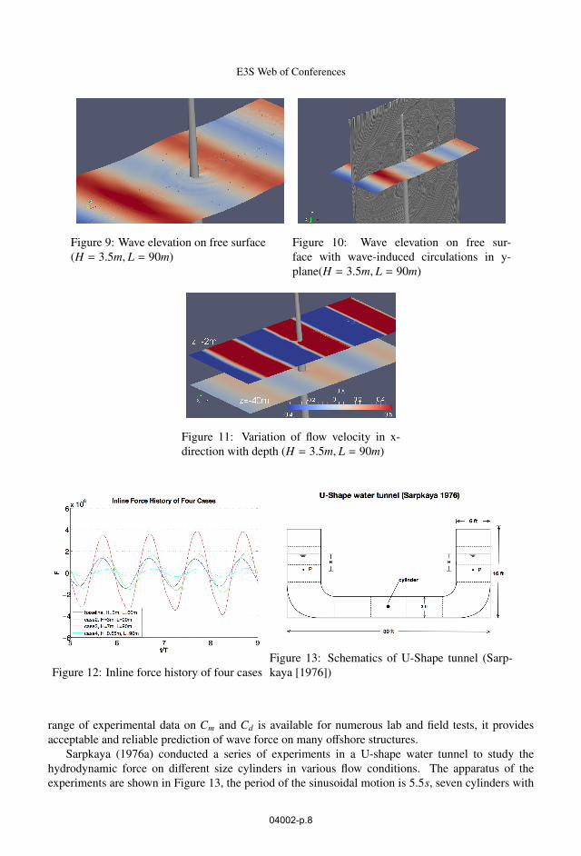
Figure 9: Wave elevation on free surface

(H = 3.5m, L = 90m)

Figure 10: Wave elevation on free sur-

face with wave-induced circulations in y-

plane(H = 3.5m, L = 90m)

Figure 11: Variation of flow velocity in x-

direction with depth (H = 3.5m, L = 90m)

Figure 12: Inline force history of four cases

Figure 13: Schematics of U-Shape tunnel (Sarp-

kaya [1976])

range of experimental data on Cm and Cd is available for numerous lab and field tests, it provides

acceptable and reliable prediction of wave force on many offshore structures.

Sarpkaya (1976a) conducted a series of experiments in a U-shape water tunnel to study the

hydrodynamic force on different size cylinders in various flow conditions. The apparatus of the

experiments are shown in Figure 13, the period of the sinusoidal motion is 5.5s, seven cylinders with

E3S Web of Conferences

04002-p.8

diameter ranging from 2 to 6.5 inches were used.

Figure 14 and 15 show part of the result from Sarpkaya’s experiments, the frequency parameter βis defined as

β = Re/K =D2

νT(8)

Figure 14: Cd versus K for various values

of β (Sarpkaya [1976])

Figure 15: Cm versus K for various values

of β (Sarpkaya [1976])

In full-scale cases, the flow around floating platform has very high Reynolds number, several

magnitudes higher than the experiments, Sarpkaya (1976b) also studied the force on cylinder at high

Reynolds number.

Figure 16: Cd versus Re for various values of β (Sarpkaya[1976])

Figure 16 and Figure 17 shows that at high Re, Cm approaches 1.8 and Cd approaches 0.65 at

various values of K. In reality, Reynolds number along the vertical length of the pile ranges from 107

near free surface to 105 at wave base, we can safely assume that

Cm = 1.8 and Cd = 0.65

2nd Symposium on OpenFOAM� in Wind Energy

04002-p.9

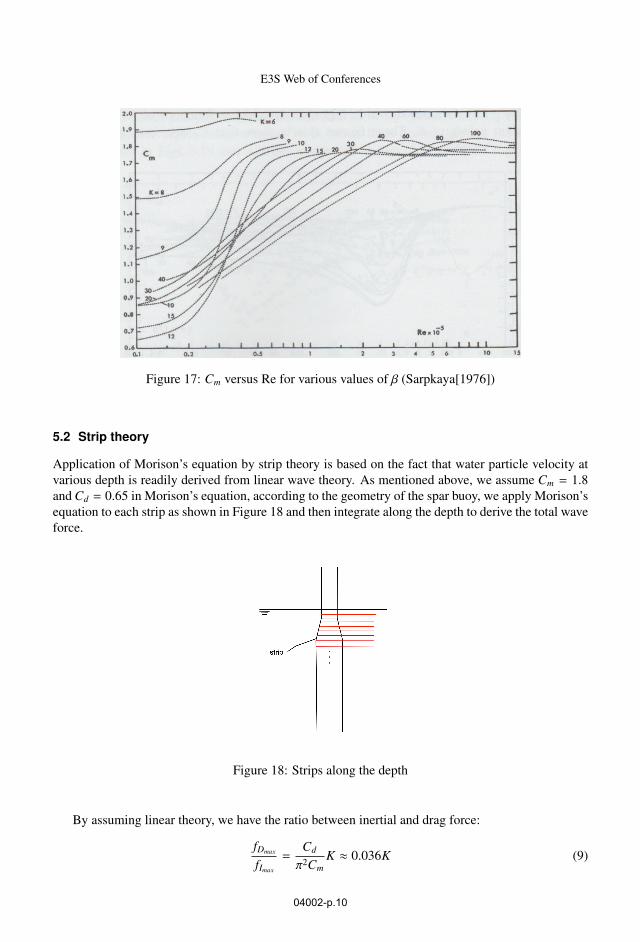
Figure 17: Cm versus Re for various values of β (Sarpkaya[1976])

5.2 Strip theory

Application of Morison’s equation by strip theory is based on the fact that water particle velocity at

various depth is readily derived from linear wave theory. As mentioned above, we assume Cm = 1.8and Cd = 0.65 in Morison’s equation, according to the geometry of the spar buoy, we apply Morison’s

equation to each strip as shown in Figure 18 and then integrate along the depth to derive the total wave

force.

Figure 18: Strips along the depth

By assuming linear theory, we have the ratio between inertial and drag force:

fDmax

fImax

=Cd

π2CmK ≈ 0.036K (9)

E3S Web of Conferences

04002-p.10

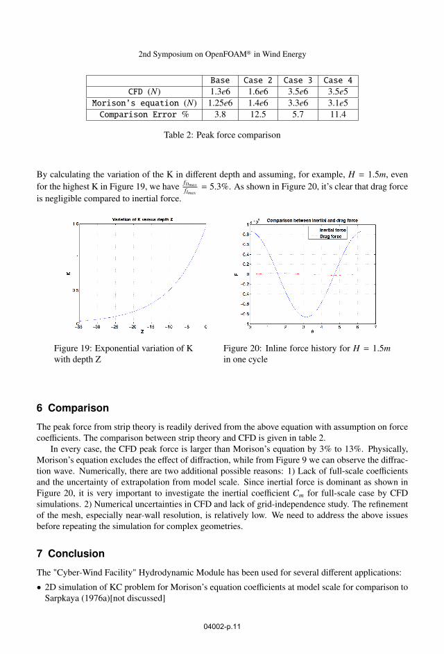
Base Case 2 Case 3 Case 4CFD (N) 1.3e6 1.6e6 3.5e6 3.5e5

Morison’s equation (N) 1.25e6 1.4e6 3.3e6 3.1e5

Comparison Error % 3.8 12.5 5.7 11.4

Table 2: Peak force comparison

By calculating the variation of the K in different depth and assuming, for example, H = 1.5m, even

for the highest K in Figure 19, we havefDmaxfImax= 5.3%. As shown in Figure 20, it’s clear that drag force

is negligible compared to inertial force.

Figure 19: Exponential variation of K

with depth Z

Figure 20: Inline force history for H = 1.5min one cycle

6 Comparison

The peak force from strip theory is readily derived from the above equation with assumption on force

coefficients. The comparison between strip theory and CFD is given in table 2.

In every case, the CFD peak force is larger than Morison’s equation by 3% to 13%. Physically,

Morison’s equation excludes the effect of diffraction, while from Figure 9 we can observe the diffrac-

tion wave. Numerically, there are two additional possible reasons: 1) Lack of full-scale coefficients

and the uncertainty of extrapolation from model scale. Since inertial force is dominant as shown in

Figure 20, it is very important to investigate the inertial coefficient Cm for full-scale case by CFD

simulations. 2) Numerical uncertainties in CFD and lack of grid-independence study. The refinement

of the mesh, especially near-wall resolution, is relatively low. We need to address the above issues

before repeating the simulation for complex geometries.

7 Conclusion

The "Cyber-Wind Facility" Hydrodynamic Module has been used for several different applications:

• 2D simulation of KC problem for Morison’s equation coefficients at model scale for comparison to

Sarpkaya (1976a)[not discussed]

2nd Symposium on OpenFOAM� in Wind Energy

04002-p.11

• Simulation of OC3 spar-buoy in waves using interFoam and waves2Foam. Conditions set to Hs

typical for future offshore-wind-plant near the coast of Virginia.

CFD simulations predict higher average peak force than Morison’s equation. The hypothesis for the

discrepancy is that diffraction effects is neglected in Morison’s equation, full-scale coefficients are

unknown, CFD accuracy not yet assessed using domain-size, time-step and grid refinement studies.

However, the use of robust HPC resources at VT-ARC give good turn-around, many cases can be

simulated in 24-hour period.

8 Future work

As a preliminary study of the module, there are many aspects need to be explored in the future, in-

cluding re-mesh for large domain which includes rotor disc; compute Morsion’s equation coefficients

at full-scale conditions, and quantify 3D and scale effects; test and debug mooring-line model; col-

laborate with CWF team members: 1) Use tightly coupled 6DOF/RANS solver (Dunbar et al., 2014)

and 2) Incorporate turbine forces (Jha et al., 2013).

References

[1] Brasseur, J., Paterson, E., Schmitz, S., Campbell, R., Vijayakumar, G., Lavely, A., ... & Haupt, S.

2013 A “Cyber Wind Facility” for HPC Wind Turbine Field Experiments, In APS March Meeting

Abstracts (Vol. 1, p. 1189).

[2] Cummins, W. 1962. The impulse response function and ship motion, David Taylor Model Basin-

DTNSRDC

[3] Campbell, R. & Paterson, E. 2011. Fluid-structure interaction analysis of flexible turbomachinery,

Journal of Fluids and Structures 27(8)

[4] Dunbar, A., Craven, B. & Paterson, E. 2014. Application of a Tightly-Coupled CFD/6-DOF Solverfor Simulating Offshore Wind Turbine Platforms, 2nd SOWE Presentation

[5] Jacobsen, N., Fuhrman D & Fredsøe, J. 2012. A wave generation toolbox for the open-sourceCFD library: OpenFoam R©

[6] Jha, P., Churchfield, M., Moriarty P., & Schmitz, S. 2013. Accuracy of State-of-the-Art Actuator-Line Modeling for Wind Turbine Wakes, 51st AIAA Aerospace Sciences Meeting

[7] Jonkman, J. 2010. Definition of the Floating System for Phase IV of OC3, Technical Report:

NREL/TP-500-47535, National Renewable Energy Laboratory

[8] Jonkman, J. 2007. Dynamics Modeling and Loads Analysis of an Offshore Floating Wind Turbine,

Technical Report: NREL/TP-500-41958, National Renewable Energy Laboratory

[9] Robertson, A., Jonkman, J., Musial, W., Vorpahl, F. & Popko, W. 2013. Offshore Code Compar-ison Collaboration, Continuation: Phase II Results of a Floating Semisubmersible Wind System,

Technical Report: NREL/CP-5000-60600, National Renewable Energy Laboratory

[10] Sarpkaya, T. 1976a. In-line and Transverse Forces on Smooth and Sand-roughened Cylinders inOscillatory Flow at High Reynolds Numbers, National Science Foundation

[11] Sarpkaya, T. 1976b. Vortex Shedding and Resistance in Harmonic Flow about Smooth andRough Circular Cylinders at High Reynolds Numbers

E3S Web of Conferences

04002-p.12