A Study of Volatility of Select Metals Traded in the ... · A Study of Volatility of Select Metals...

ISSN: 0971-1023 | NMIMS Management Review Volume XXXV | Issue 4 | January 2018

A Study of Volatility of Select Metals Traded in the Indian Commodity Market

50

A Study of Volatility of Select Metals Traded in the Indian Commodity Market

Shubhangi Jore¹

Varsha Shrivastava²

Abstract

Commodities such as gold, silver and copper have

drawn considerable attention with respect to their

price volatility. The spot prices of precious metals (gold

and silver) not only redirects us to review the current

supply and demand condition, but also reveals the

predictions of future inflation and the general business

and economic environment. The commodity market is

where raw or primary products are exchanged or

transacted. A commodity is classified as every kind of

movable property; it includes only physical products

such as food, electricity, metals, etc. and excludes

services – government services, investments, debt,

actionable claims, money, securities, etc. The present

study attempts to assess the time-varying price

¹ Associate Professor, SBM, Indore,SVKM's NMIMS University ² Data Researcher, S&P Global Market Intelligence, Ahmedabad

volatility of gold, silver and copper and the nature of

the volatility process. The results indicate presence of

persistence in price volatility as per the estimation

outputs of GARCH (1, 1) model for silver and copper

metals. On the basis of the estimated results of GARCH

model, it can be concluded that returns of silver and

copper metals were highly volatile as compared to

returns of gold during the period January 2014 to

December 2016 while considering daily returns. It can

also be concluded that copper is more volatile

compared to gold and silver.

Key words: ARCH, GARCH model, Volatility, Metals

Volume XXXV | Issue 4 | January 2018 in the Indian Commodity Market

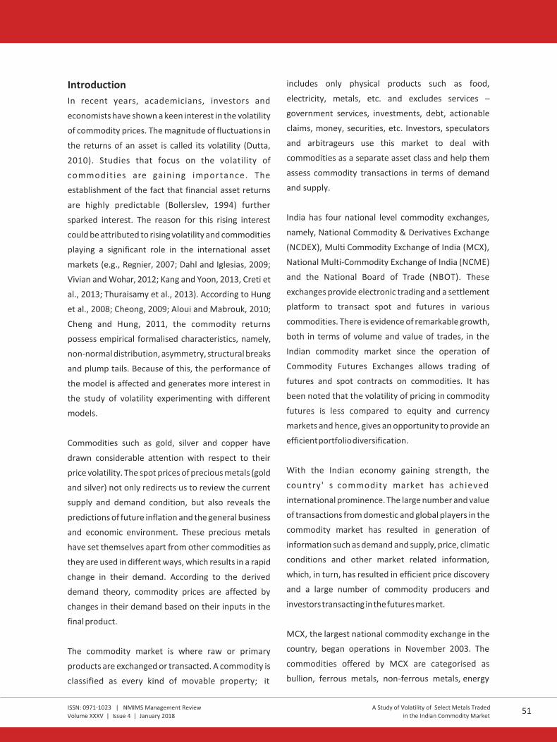
Introduction

In recent years, academicians, investors and

economists have shown a keen interest in the volatility

of commodity prices. The magnitude of fluctuations in

the returns of an asset is called its volatility (Dutta,

2010). Studies that focus on the volatility of

commodit ies are gaining importance. The

establishment of the fact that financial asset returns

are highly predictable (Bollerslev, 1994) further

sparked interest. The reason for this rising interest

could be attributed to rising volatility and commodities

playing a significant role in the international asset

markets (e.g., Regnier, 2007; Dahl and Iglesias, 2009;

Vivian and Wohar, 2012; Kang and Yoon, 2013, Creti et

al., 2013; Thuraisamy et al., 2013). According to Hung

et al., 2008; Cheong, 2009; Aloui and Mabrouk, 2010;

Cheng and Hung, 2011, the commodity returns

possess empirical formalised characteristics, namely,

non-normal distribution, asymmetry, structural breaks

and plump tails. Because of this, the performance of

the model is affected and generates more interest in

the study of volatility experimenting with different

models.

Commodities such as gold, silver and copper have

drawn considerable attention with respect to their

price volatility. The spot prices of precious metals (gold

and silver) not only redirects us to review the current

supply and demand condition, but also reveals the

predictions of future inflation and the general business

and economic environment. These precious metals

have set themselves apart from other commodities as

they are used in different ways, which results in a rapid

change in their demand. According to the derived

demand theory, commodity prices are affected by

changes in their demand based on their inputs in the

final product.

The commodity market is where raw or primary

products are exchanged or transacted. A commodity is

classified as every kind of movable property; it

includes only physical products such as food,

electricity, metals, etc. and excludes services –

government services, investments, debt, actionable

claims, money, securities, etc. Investors, speculators

and arbitrageurs use this market to deal with

commodities as a separate asset class and help them

assess commodity transactions in terms of demand

and supply.

India has four national level commodity exchanges,

namely, National Commodity & Derivatives Exchange

(NCDEX), Multi Commodity Exchange of India (MCX),

National Multi-Commodity Exchange of India (NCME)

and the National Board of Trade (NBOT). These

exchanges provide electronic trading and a settlement

platform to transact spot and futures in various

commodities. There is evidence of remarkable growth,

both in terms of volume and value of trades, in the

Indian commodity market since the operation of

Commodity Futures Exchanges allows trading of

futures and spot contracts on commodities. It has

been noted that the volatility of pricing in commodity

futures is less compared to equity and currency

markets and hence, gives an opportunity to provide an

efficient portfolio diversification.

With the Indian economy gaining strength, the

country' s commodity market has achieved

international prominence. The large number and value

of transactions from domestic and global players in the

commodity market has resulted in generation of

information such as demand and supply, price, climatic

conditions and other market related information,

which, in turn, has resulted in efficient price discovery

and a large number of commodity producers and

investors transacting in the futures market.

MCX, the largest national commodity exchange in the

country, began operations in November 2003. The

commodities offered by MCX are categorised as

bullion, ferrous metals, non-ferrous metals, energy

ISSN: 0971-1023 | NMIMS Management Review A Study of Volatility of Select Metals Traded 51


and agriculture. This paper is an attempt to examine

the price volatility of three commodities, namely, gold,

silver and copper. These commodities have been

selected since they are highly traded on the world

commodity markets and have different economic

uses. These commodities are important in terms of

their industrial usage with strong linkages as add-ons

and substitutes across the entire economy. The price

movements and volatility are considered to follow the

business cycle. Gold is considered a precious metal; it

is not only classified as a commodity, but also as one of

the strongest monetary assets (Tulley and Lucey,

2007). Gold is a multifaceted metal which can be

stored as wealth, medium of exchange and a unit of

value (Goodman, 1956; Solt and Swanson, 1981). The

price volatility during the period January 2014 to

December 2016 of the commodities under

consideration can be viewed in Figure 1.

Figure 1: Closing price of Gold, Silver and Copper -

01 January, 2014 to 31 December, 2016

Gold

Silver

Copper

Source: Authors' computations using data from Multi Commodity Exchange (MCX) of India

To measure volatility, the generalised autoregressive

conditional heteroscedasticity (GARCH) scheme was

developed during the early 1980s; this became

instrumental in popularising econometric modelling.

Chipili (2012) studied volatility in the exchange rate

and revealed that GARCH models help to estimate the

path for time-varying conditional variance of the

exchange rate. It also enabled the researcher to

capture the appropriate conditional volatility present

in the exchange rate.

Review of Literature

In the past, many researchers have shown keen

interest in studying the volatility of the stock market,

exchange rates and prices of commodities with

reference to different regions. This section gives a brief

overview of the findings and suggestions. Though

there is extensive research available on this subject,

the authors have considered only the latest work. The

literature review on the existing topic is significant

since it provides the basis to formulate the problem

and offer the analysis.

Research on exchange rate volatility has been

conducted in different regions and countries; some of

these are briefly reviewed in the present section. One

of the upcoming mediums of exchange, Bitcoin, is

gaining attention across the world. The empirical work

for fitting the daily Bitcoin exchange rate returns by Liu

52 ISSN: 0971-1023 | NMIMS Management Review A Study of Volatility of Select Metals Traded


et al. (2017) compared the performance of a newly-

developed heavy-tailed distribution, the normal

reciprocal inverse Gaussian (NRIG), with the most

popular heavy-tailed distribution, the Student's t

distribution, under the GARCH framework. It revealed

that heavy-tailed distribution performance of daily

Bitcoin exchange rate returns was captured in a better

way compared to the standard normal distribution. It

concluded that the old fashioned Student's t

distribution performed better than the new heavy-

tailed distribution.

Omari et al. (2017) applied generalised autoregressive

conditional heteroscedastic models in modelling

USD/ KES exchange rate volatility using daily

observations over the period starting 3rd January 2003

to 31st December 2015. Authors have utilised both

symmetric and asymmetric models that capture most

of the formalised facts about exchange rate returns

such as volatility clustering and leverage effect. The

volatility has been tested by applying the symmetric

GARCH (1, 1) and GARCH-M models as well as the

asymmetric EGARCH (1, 1), GJR-GARCH (1, 1) and

APARCH (1, 1) models with different residual

distributions.

Epaphra (2017) studied the modelling of exchange

rate volatility for Tanzania. To detect whether there

exists a symmetric effect in exchange rate data, the

paper applied both the autoregressive conditional

heteroscedastic (ARCH) and GARCH models. The

results of the study revealed that exchange rate data

exhibits the application of ARCH methodology. The

application of methodology was justified by empirical

regularities such as clustering volatility, non-

stationarity, non-normality and serial correlation.

For financial traders, examining volatility in the

commodity market is an interesting subject. One may

find a large number of speculative trades in metal

prices as these are generally subject to fluctuation

(Moore and Cullen, 1995). In recent years, there has

been an increasing amount of speculative activities in

emerging economies, which has led to more

uncertainty and greater volatility in these markets (Gil-

Alana and Tripathy, 2014). There is much lesser

research carried out to examine volatility in non-

energy commodity markets, metals and agriculture as

compared to stock and energy markets (Behmiri and

Manera, 2015). In this framework, Mackenzie et al.

(2001) have investigated the volatility of precious

metal prices and used the univariate power ARCH

model. The results reveal that there is no asymmetric

effect in metal markets. To examine the volatility of

gold, silver and copper prices while controlling the

shocks of oil prices and the US interest rate changes,

Hammoudeh and Yuan (2008) applied the univariate

GARCH-type model. To explore the volatility of

precious metal prices pre and post the global and Asian

financial crises, Morales and O'Callaghan (2011)

utilised the GARCH and the EGARCH models. The

results showed a strong evidence of persistent

volatility in the metal market during the global

financial crisis; however, volatility was very weak

during the Asian financial crisis.

One of the latest research studies by Kruse et al.

(2017) utilised the GARCH model for platinum returns.

The findings showed that the NRIG distribution

performed better than the most widely-used heavy-

tailed distribution, the Student's t distribution.

Goodwin (2012), in his research, assessed the

suitability of standard GARCH (1,1) models to model

(in-sample) and forecast (out-of-sample) the volatility

of copper spot price returns in four equally large sub-

samples during the period July 21, 1993 to March 22,

2012. The results revealed that it was highly

satisfactory to utilise the GARCH models to model the

conditional variance. It was also found that presence

of ARCH effects was also significant. In out-of-sample

forecasting, the GARCH models dominated a Random



Walk model across all four sub-samples. The study

concluded that it could be interpreted that the

standard GARCH (1,1) model was sufficient.

The assessment of the asymmetry and long memory

effects in modelling the volatility of crude oil, natural

gas, gold and silver prices was done by Chkili et al.

(2014) using the GARCH models. The authors arrived

at the conclusion that there was lower volatility

persistence in the gold and silver markets compared to

the prices of oil and natural gas. Gil-Alana and Tripathy

(2014) applied the GARCH-type models to examine

the volatility persistence and leverage effect for non-

precious metal markets in India. The authors reported

existence of a high degree of volatility persistence in all

metals; the asymmetric effect was established for

seven metals according to the TGARCH model and for

ten metals according to the EGARCH model. To

examine volatility spillovers between non-precious

metals, Todorova et al. (2014) used the multivariate

Heterogeneous Auto regressive (HAR) model. The

study concluded, on one side, that volatility of other

industrial metals contains useful information for

future price volatility. On the other side, the own

dynamics of each metal were mostly appropriate to

elucidate the future daily and weekly volatility.

Cochran et al. (2015) examined the role of higher

order moments in the returns of four important

metals, namely, aluminium, copper, gold and silver.

The analysis of the return series was conducted using

the asymmetric GARCH (AGARCH) model with a

conditional skewed generalised-t (SGT) distribution.

The AGARCH model with the SGT distribution

appeared to have the best fit for all metals examined,

except gold.

Ma et al. (2017) investigated the widely-used GARCH

model in risk management of palladium spot returns.

The authors followed the work done by Guo (2017a)

and compared two types of heavy-tailed distribution -

the Student's t distribution and the normal reciprocal

inverse Gaussian (NRIG) distribution, under the

GARCH framework. The researchers were specifically

interested in identifying the difference between

empirical performances of quantifying palladium spot

volatilities for the two distributions. The results

showed that the newly-developed distribution, the

NRIG, was unable to outperform the older fashioned

Student's t distribution.

Saranya (2015), in his research, focused on the futures

market for selected non-agricultural commodities. The

study was based on data relating to futures prices and

spot prices of eleven non-agricultural commodities,

which included energy and precious metals. Data was

collected from the website of one of the leading

commodity exchanges in India for the period 2008 to

2014. The analysis of the study was based on the use of

certain econometric tools such as unit root test to test

the stationarity and Granger causality test to measure

the lead-lag relationship between the spot and futures

returns. To examine the volatility in the spot and

futures returns, GARCH model was used. The study

concluded that there exists a unidirectional causality in

selected commodities like tin and silver while there

exists a bi-directional causality in copper. In case of

other commodities, namely aluminium, copper, lead,

zinc, nickel, gold and silver, the coefficient of trade

volume was positive and open interest was negative.

The study confirmed the existence of volatility in

selected non-agricultural commodities in both the

spot and futures market.

Sinha and Mathur (2013) studied the volatility of five

metals, namely, nickel, lead, zinc, aluminium and

copper traded on the Multi Commodity Exchange

(MCX). The data was collected for the period

November 2007 to January 2013. The objective of the

study was to assess the impact of the global financial

crisis on trading of base metals. The GARCH model was

applied to assess the volatility of metals. The results



revealed that there existed short term persistence in

price volatility of metals and daily price volatility of

base metals was influenced by the global financial

crisis.

Cochran et al. (2012) examined the volatility of four

precious metals, namely, copper, platinum, gold and

silver. The returns and long-term properties of return

volatility were analysed using the FIGARCH model.

The results of the study revealed a significant

relationship between price volatility of these metals

and lagged implied volatility of the equity market in

India. The results were based on modified GARCH (1,

1) model. The research concluded that there exists the

impact of financial crisis on return volatility of metals.

On similar lines, Morales and Callaghan (2011)

examined the nature of volatility spill-overs between

returns of four precious metals - gold, silver, palladium

and platinum. The study considered the data during

the Asian and the global financial crisis using the

GARCH and EGARCH models. The results of the study

revealed that the returns of precious metals were

persistent during the global financial crisis while it was

weak for volatility persistence during the Asian crisis in

the 1990s.

Arouri et al (2012) explored the existence of long

range dependence in the daily conditional return and

volatility processes for precious metals, namely gold,

silver, platinum and palladium. The results revealed

that during the periods of crisis, platinum was not an

appropriate hedging instrument while gold served as a

better instrument. In terms of predictive power for

volatility and returns, the FIGARCH model was the

most effective.

In the Indian context, time varying volatility

seasonality and risk-return relationships in a GARCH-

in-mean framework for the Indian commodity market

was examined by Kumar and Singh (2008), while

Mahalakshmi et al. (2012) inspected the behaviour of

commodity derivatives in the Indian market from the

Composite Commodity Derivative Index of Multi

Commodity Exchange (MCX) using ARCH/GARCH

models.

According to Sharma and Kumar (2001), the changes

in price and instability in commodities impose a large

amount of overhead on both the producers and

consumers. Producers of the commodity suffer if the

price contracts below the cost of production and

consumers are at a disadvantage if the price surpasses

a certain level. While low prices can be beneficial to

consumers while encouraging them to buy more, high

prices result in higher producers' gains. But a sudden

fall or increase in commodity prices can be serious and

may create problems for the economy. The variations

in price movements have rigorous consequences such

as higher speculation, formation of flawed policies on

pricing and so on.

Engle (1982) and Bollerslev (1986) have developed the

popular models of volatility clustering. To capture the

volatility clusters in financial time series, the ARCH

models (Engle, 1982) and generalised ARCH (GARCH)

models (Bollerslev, 1986) have been comprehensively

used. It has been confirmed by Bollerslev et al., (1994)

that the GARCH-type models are superior to predict

volatility in comparison to the naïve historical average,

moving average and exponentially weighted moving

average (EWMA) models. There are specific models to

predict the variance and conditional variance. The

Threshold GARCH model (TGARCH) (Glosten et al.,

1993) and Exponential GARCH (EGARCH) model

(Nelson, 1991) are used to predict conditional

variance and are relatively steady models. This study

attempts to use ARCH and GARCH models to predict

conditional variance.

To estimate the volatility of fifty individual stocks,

Karmakar (2005) used conditional volatility models.

The study revealed that the GARCH (1,1) model



provided a reasonably good forecast. Another study by

Krishnan (2010) was based on high frequency data for

the Indian stock market. It attempted to observe the

way larger and smaller errors cluster together using

autoregressive conditional heteroscedasticity models.

The study included stock prices of SBI and TATA to

observe the volatility cluster.

The volatility in the commodity market should be

studied to benefit not only those who participate in

research is explanatory in nature. The study spans the

period 01 January, 2014 to 31 December, 2016 of daily

data of the spot prices of gold, silver and copper

collected from Multi Commodity Exchange (MCX) of

India to determine the volatility of commodity returns.

A total of 772 observations of spot prices for the three

metals, i.e. gold, silver and copper have been used for

the analysis. These prices are converted to returns by

means of first differences of the log-transformed data

using equation (1).

this market, but also for the economy as a whole. The

commodity market in India is still at a nascent stage of

development and there is huge potential to explore

and study the behaviour of this market, especially

since the Indian economy is an agriculture-based

economy. Gold, silver and copper commodities are

among the most traded on the world commodity

markets and also have different economic uses.

Through their important industrial uses, these

commodities have strong linkages as complements

and substitutes with the overall economy, and their

prices and volatilities move in sync with the business

cycle. This study attempts to assess the time varying

price volatility of gold, silver and copper, and the

nature of the volatility process.

Methodology

According to Omari et al. (2017), to measure volatility,

traditional methods such as variance or standard

deviation are lacking with respect to capturing the

characteristics exhibited by financial time series data.

The characteristics such as time varying volatility,

volatility clustering, excess kurtosis, heavy tailed

distribution and long memory properties can only be

captured using the most commonly used models,

n a m e l y, t h e A u t o r e g r e s s i v e C o n d i t i o n a l

Hete ro sc edast ic i ty ( A R C H ) model and i t s

generalisation, and the Generalised Autoregressive

Conditional Heteroscedasticity (GARCH) models.

The present work is based on empirical study and the

The data is analysed to study the extent of volatility

persistence using the Autoregressive Conditional

Heteroscedasticity ( A R C H ) model and i t s

generalisation, and the Generalised Autoregressive

Conditional Heteroscedasticity (GARCH) models.

Non-Normality Distribution of Fat Tails

The assessment of the extent of deviation of Skewness

and Kurtosis from the normality assumption of

symmetry (Skewness is zero) and fixed peak value of

three is done by the statistics proposed by Bera and

Jarque (1982). The null hypothesis (H0) for this test

states that the distribution is normally distributed. The

Jarque-Bera (JB) test statistics is calculated as--

where, is the sample Skewness.

Skewness or the third moment of the distribution

measures the asymmetry while the fourth moment or

Kurtosis measures the peakness of the distribution

and is denoted by K and calculated as

the sample size, is the sample mean and is the

sample standard deviation. For large sample size, JB

statistics follows chi-square distribution with two

degrees of freedom. If the value of p is less than 0.01

then the null hypothesis (H₀) is rejected and it is

interpreted that the distribution does not follow

normal distribution.



Parametric Volatility Models

The time series volatility Auto Regressive Conditional

Heteroscedasticity (ARCH) model as designed by

Engle (1982) assumes the unconditional error variance

to be constant, and the conditional variance is

assumed to be dependent on past realisations of the

error process. The ARCH model was further

generalised by Bollerslev (1986) and Taylor (1986) to

generate the GARCH model. To study volatility

persistence and spill-over effects through financial

g e n e r a l i s e d a u t o r e g r e s s i v e c o n d i t i o n a l

heteroscedasticity (GARCH) model can be estimated.

The Generalised Autoregressive Conditional

Heteroscedasticity (GARCH) Model

The GARCH model is described by a linear function of

conditional variance of its own lags. The general form

of the GARCH (p, q) model is given by:

series, there are a number of other methods, but the

ARCH/GARCH models appear to be the most

prevalent ones. The models are briefly described

below.

T h e A u t o r e g r e s s i v e C o n d i t i o n a l

Heteroscedasticity (ARCH) Model

The ARCH model describes the return series of a

financial time series as a linear function of its lag term.

In an attempt to determine the ARCH effect for metal

prices, the following time series least square

regression equation (3) is estimated. The null

hypothesis (H0) assumes that there is no Arch effect on

the return series of financial data against the

alternative hypothesis (H1) that there is an Arch effect

on the return series.

where,

Yt denotes returns of the commodity

a denotes constant quantity

Yt-1denotes lag term of the returns of the commodity

t = 1, 2, …

After running the least square regression equation (3),

the values of n and R2 are noted and chi-square (χ

2)

statistic is calculated as If the

calculated value of χ2 is less than the critical value, then

we may accept the null hypothesis. The presence

of ARCH effect on the return series indicates that

there exists persistence volatility in the series

and further,

where, rt is the log of returns of the time series data at

time t, µ is the mean of return series, yt is the error term

from the mean equation and it can split into error term

ԑt and a time dependent standard deviation σt, ԑt is

assumed to follow (iid) with zero mean, which is

assumed to have normal distribution, t distribution

and skew t distribution and

with constraints

The basic GARCH (1, 1) model fits in most of the

empirical applications of the majority of financial time

series reasonably well. The GARCH (1, 1) model is

given by the following equation:

The following restrictions are imposed to guarantee a

positive variance at all instances,

In most of the cases, to analyse the financial

time series data and to estimate the conditional

volatility, the basic GARCH model provides a

reasonably good model (Omari et al, 2017). However,


looking to different aspects and dynamics, there is

scope for improvement in the GARCH (p, q) model

introduced by Bolleslev (1986), which can better

capture these characteristics of a particular financial

time series.

Diagnostic Tests

Diagnostic test is performed in two parts; the first part

gets fulfilled if residuals follow mean 0 and variance 1,

and the second part is fulfilled if the residuals are not

auto-correlated. To diagnose the first part, the

condition of normality of residuals is checked; if it

follows Mean 0 and Variance 1, then the condition of

first diagnostic test is fulfilled. In the second, the null

hypothesis of no autocorrelation using Ljung – Box (Q)

Statistics is tested. If significant value (p) is more than

0.01, then we accept the null hypothesis that the

residuals are not auto-correlated.

Results And Analysis

Daily prices of commodities have been converted to

daily returns. This study utilises the logarithmic

difference of prices of two successive periods for the

calculation of rate of return. As we move up and down,

the converted data of return series is symmetric

between the movements. If Pt denotes closing price of

the commodity on date t and Pt-1be that for its previous

day, then the one-day return on the commodity

market portfolio is calculated as given in equation (7).

Please note here that the intervening weekend or

commodity exchange holidays are omitted.

Where, ln (w) is the natural logarithm of 'w.'

return is the most volatile series during the sample

period. Returns are positively skewed in all metals and

a fat tailed distribution has a value of kurtosis that

exceeds 3. All the three metal return series have high

kurtosis with the highest being 7.24 corresponding to

gold returns; thus, results indicate that all metal return

series are leptokurtic (fat tailed). According to Watkins

and McAleer (2008), if the distribution is leptokurtic,

then AR (1) - GARCH (1, 1) model is appropriate to

describe the conditional variance of the data series.

The authors further add that these models represent

the data in terms of rolling diagnostic tests for

normality, serial correlation and existence of ARCH

effects. The authors commented that GARCH (1, 1)

model is the most commonly used volatility model.

As the return series of these metals is leptokurtic in

nature, they have higher probability of securing large

positive or large negative values of returns. To test

further the normality of the return series of gold, silver

and copper, the Jarque-Bera test is applied. The p-

value of Jarque-Bera test is zero for return series of the

metals, thus rejecting the presence of normality.

Rejection of normality of return series confirms the

assumption that the model selected should account

for the heavy-tail phenomenon.

Initially, the statistical features are assessed and Table

1 describes the summary statistics of return series of

the spot prices of metals. The results suggest that

copper possesses the highest mean daily return while

gold has the poorest performance in terms of mean

daily return. In terms of volatility, the silver metal

58 ISSN: 0971-1023 | NMIMS Management Review

A Study of Volatility of Select Metals Traded


Table 1: Summary Statistics of Return Series of Base Metals

Gold Silver Copper

Mean -7.83e-06 -7.15e-05 -0.000232

Median -0.000331 -0.000256 -0.000641

Std. Deviation 0.007389 0.011485 0.0103081

Maximum 0.051452 0.0518680 0.054550

Minimum -0.025016 -0.052026 -0.061280

Skewness 0.719386 0.312268 0.149452

Kurtosis 7.240880 5.118706 6.188898

Jarque-Bera (JB) 644.2708 156.7367 329.5515

J-B(P-Values) 0.00 0.00 0.00

Std dev./ mean -943.68 -160.63 -44.43

ADF (0) -23.589 -22.533 -22.856

ADF (P-value) 0.000 0.000 0.000

Source: Authors' calculations

Figure 2, 4 and 6 display the closing price of gold, silver

and copper. All mean series move in a similar way.

There are considerable ups and downs in the closing

prices of gold, silver and copper over the sample

period. In general, the volatility in silver and copper

seems to be more evident in comparison to gold. To

see it more intensely, Figure 3, 5 and 7 plot the changes

Figure 2: Closing prices of Gold - 01 January, 2014 to 31 December, 2016

in the closing prices of these metals. From these

figures, it is apparent that the volatility appears in

clusters and also provides evidence that time varying

volatility in daily closing prices of metals is empirically

shown as return clustering. This feature is referred to

as the presence of ARCH / GARCH effects (Humala &

Rodríguez, 2010).

Figure 3: Change in Closing prices of Gold - 01 January, 2014 to 31 December, 2016


Source: Author's computations using data from Multi Commodity Exchange (MCX) of India

ISSN: 0971-1023 | NMIMS Management Review A Study of Volatility of Select Metals Traded

59


Figure 4: Closing prices of Silver - 01 January, 2014 to 31 December, 2016

Figure 7: Change in Closing prices of Copper - Jan 2014 to Jan 2016


Figure 5: Change in Closing prices of Silver - Jan 2014 to Jan 2016


A prescribed statistical test is examined further to

support the descriptive statistics and graphical tests of

persistence. Augmented Dickey Fuller Test (ADF)

(Table 2) is employed to check the stationarity of

return series of gold, silver and copper.


Figure 6: Closing prices of Copper -

01 January, 2014 to 31 December, 2016




Table 2 (a): Augmented Dickey-Fuller test of the return series of Gold

Table 2 (b): Augmented Dickey-Fuller test of the return series of Silver

Table 2 (c): Augmented Dickey-Fuller test of the return series of Copper

The test assumes the null hypothesis that the time

series has a unit root (non-stationary). The ADF test

statistic -23.589, -22.533 and -22.129 (p = 0.000)

respectively for gold, silver and copper return series

indicates that the null hypothesis is rejected for all the

considered metals i.e. return series does not have a

unit root. Thus, these metal return series are

stationary and hence, we can proceed further to test

its volatility using ARCH and GARCH models.

The volatility has been analysed using the standard

GARCH model. Before estimating the GARCH models,

we must check for the presence of the ARCH effect to

check the short-term volatility persistence. This check

must be carried out before and after the model

estimations have been performed to ascertain

whether or not any ARCH effect exists or remains; if it

remains, it indicates that the variance equations are

still mis-specified. If the ARCH effect is present, then

the data is further tested for its volatility using GARCH

model to check whether there is long-term volatility

persistence in the return series.

Estimation of Volatility Model

A simple AR (1) process with an intercept was

estimated in order to determine the best fit linear

mean function for each of the series. In an attempt to

determine the ARCH effect for gold, silver and copper

return series, time series least square regression

equation (8) has been fitted.



The significance of this equation was then established and the error term of each mean equation was converted

into the particular residual (ԑt).The estimated results are shown in the Table 3.

Table 3: Estimation of ARCH effect for Gold, Silver and Copper

As depicted from Table 3, ARCH effect does not exist

for gold return series, which indicates that there is no

short-term volatility persistence in the return series

and hence, further GARCH model is not estimated for

gold returns. On the other hand, there exists short-

term volatility persistence in silver and copper return

series as ARCH effect is significant in these two metal

return series. Further, the GARCH model is estimated

for silver and copper return series to explore long-term

volatility persistence. To understand the direction of

volatility of these two metal return series, a normal

GARCH (1,1) is run. The equation (5 and 6) has been

fitted. Table 4 reports the results of GARCH (1, 1)

estimation results for silver and copper daily return

series.




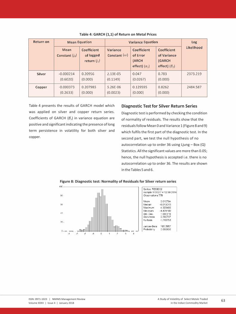
Table 4: GARCH (1,1) of Return on Metal Prices

Table 4 presents the results of GARCH model which

was applied on silver and copper return series.

Coefficients of GARCH (β2) in variance equation are

positive and significant indicating the presence of long

term persistence in volatility for both silver and

copper.

Diagnostic Test for Silver Return Series

Diagnostic test is performed by checking the condition

of normality of residuals. The results show that the

residuals follow Mean 0 and Variance 1 (Figure 8 and 9)

which fulfils the first part of the diagnostic test. In the

second part, we test the null hypothesis of no

autocorrelation up to order 36 using Ljung – Box (Q)

Statistics. All the significant values are more than 0.05;

hence, the null hypothesis is accepted i.e. there is no

autocorrelation up to order 36. The results are shown

in the Tables 5 and 6.

Figure 8: Diagnostic test: Normality of Residuals for Silver return series

ISSN: 0971-1023 | NMIMS Management Review A Study of Volatility of Select Metals Traded

63


Table 5: Q STATISTIC (Correlogram of Squared residuals)

Diagnostic Test for Copper Return Series

Figure 9: Diagnostic test: Normality of Residuals for Copper return series



Table 6: Q STATISTIC (Correlogram of Squared residuals)

Conclusion

The key objective of this paper was to study the

volatility of gold, silver and copper metals in the

commodity market. After a comprehensive review of

literature and studying the variations in the prices

using econometric models as detailed in the previous

sections of this paper, it can be concluded that there

was presence of persistence in price volatility as per

the estimation outputs of GARCH (1, 1) model for

silver and copper metals. On the basis of the estimated

results of GARCH model, it can be concluded that

returns of silver and copper metal were highly volatile

as compared to returns of gold during the period

January 2014 to December 2016, taking daily returns.

It can also be concluded that copper is more volatile in

comparison to gold and silver. The results of the

present study can be used to predict the volatility in

prices of silver and copper metals by the Indian

manufacturing sector.



Limitatons

The results of the study can be used taking the

following limitations into consideration. The data span

considers daily closing price of metals for three years

only. The present empirical research focused only on

the volatility of return series of three metals - gold,

silver and copper, and therefore, the findings cannot

be generalised to other metals. The study is based

only on the multi commodity exchange (MCX) index

while other indices such BSE and NSE are not used.

There are other prices available under commodity

derivatives like forwards, futures, options and swaps,

but the focus of this research is on the spot prices only.

A number of commodities traded in the category of

future commodity derivatives like agro-based

commodities, soft commodities, livestock, energy,

precious metals, to name a few, can also be explored.

Only GARCH (1, 1) model is used to study the price

volatility of gold, silver and copper while the inclusion

of other asymmetric GARCH-type models, testing and

comparing their predictive performance can extend

the current study further.

Implications

The findings of the present study indicate the presence

of asymmetry and persistence in volatility, which have

important implications. Precise modelling of volatility

in the commodity market is a critical subject matter. It

can affect the portfolio allocation decision of investors,

value-at-risk management, the industrial production

of manufacturers and ultimately the economic growth

pattern of nations. Hence, from the point of view of

policy-makers, such volatility models increase the

ability to generate more accurate out-of-sample

forecasting of prices and financial traders are

facilitated by the value-at-risk management strategies.

This study offers adequate scope to undertake further

research in related fields. Instead of considering

precious metals, the study can be extended to

agricultural commodities, ferrous, non-ferrous metals

to name a few. This will enable a researcher to study

the market efficiency and testing of inter-market co-

integration. The study can further be extended by

conducting a comparative analysis of domestic and

international commodity markets of comparable

magnitude and activity. It can also be extended to

understand the short-term volatility using high

frequency data, which can be a matter of concern to

traders investing in the commodities market.



References

• Aloui, C., Mabrouk, S., (2010). “Value-at-risk estimations of energy commodities via long-memory, asymmetry

and fat-tailed GARCH models.”Energy Policy 38:2326-2339.

• Behmiri, N. B., M. Manera (2015). “The role of outliers and oil price shocks on volatility of metal

prices.”Resources Policy, 46:139-150.

• Bera, A.K. and Jarque, C.M. (1982). “Model Specification Tests: A Simultaneous Approach.” Journal of

Econometrics 20:59-82. https://doi.org/10.1016/0304-4076(82)90103-8

• Bollerslev, T., (1986). “Generalised autoregressive conditional heteroscedasticity.” Econometrica 31 (302–

327):2–27.

• Bollerslev, T., Engle, R.F. and Nelson, D.B. (1994), “ARCH Models” in R. F. Engle & D.Mc Faddeln (eds) Handbook

of EEconometrics, Vol– IV, Amsterdam, Nork – Holland.

• Cheong, C.W., (2009). “Modeling and forecasting crude oil markets using ARCH-type models.” Energy Policy 37:

2346–2355.

• Cheng, W.H., Hung, J.C., (2011), “Skewness and leptokurtosis in GARCH-typed VaR estimation of petroleum and

metal asset returns.” Journal of Empirical Finance 18: 160-173.

• Chkili, W., Hammoudeh, S., Nguyen, D. K., (2014). “Volatility forecasting and risk management for commodity

markets in the presence of asymmetry and long memory.” Energy Economics 41:1–18.

• Chipili, J.M. (2012). “Modeling Exchange Rate Volatility in Zambia.” The African Finance Journal 14:85-107.

http://hdl.handle.net/10520/EJC126376.

• Cochran, S.J., Mansur I., and Odusami B. (2012). “Volatility persistence in metal returns: A FIGARCH

approach.”Journal of Economicsand Business 64: 287-305.

• Cochran, S.J., Mansur I., and Odusami B. (2015). “Conditional higher order moments in metal asset

returns.”Quantitative Finance, DOI: 10.1080/14697688.2015.1019357.

• Creti, A., Joëts, M., Mignon, V., (2013). “On the links between stock and commodity markets' volatility.” Energy

Economics 37:16-28.

• Dahl, C.M., Iglesias, E.M., (2009). “Volatility spill-overs in commodity spot prices: new empirical results.”

Economic Modelling 26: 601-607.

• Dutta Abhijit (2010). “A Study of the NSE's Volatility for Very Small Period using Asymmetric GARCH Models.”

Vilakshan, XIMB Journal of Management, September: 107-120.

• Engle, R.F., (1982). “Autoregressive conditional heteroscedasticity with estimates of the variance of United

Kingdom inflation.” Econometrica 50:987–1007.

• Epaphra, M. (2017). “Modeling Exchange Rate Volatility: Application of the GARCH and EGARCH Models.”

Journal of Mathematical Finance 7:121-143. https://doi.org/10.4236/jmf.2017.71007

• Gil-Alana, L.A., Tripathy, T., (2014). “Modelling volatility persistence and asymmetry: a Study on selected Indian

nonferrous metal markets.” Resource Policy 41:31–39.

• Goodman, B., (1956). “The price of gold and international liquidity.” Journal of Finance 11:15–28.

• Goodwin, D. (2012). Modellingand Forecasting Volatility in Copper Price Returns with GARCH Models. Bachelor

Thesis: School of Economics and Management, Lund University, Department of Economics.

• Guo, Z. (2017a). Empirical Performanceof GARCH Modelswith Heavy-tailed Innovations, Working paper.

• Hammoudeh, S., Yuan, Y., (2008). “Metal volatility in presence of oil and interest rate shocks.” Energy Economics

30:606–620.

• Humala, A. and Rodríguez, G. (2010). Some Stylized Facts of Returns in the Foreign Exchange and Stock Markets.

Peru. Serie de Documentos de Trabajo, Working Paper Series.

• Hung, J.C., Lee, M.C., Liu, H.C., (2008). “Estimation of value-at-risk for energy commodities via fat tailed GARCH


http://hdl.handle.net/10520/EJC126376


models.” Energy Economics 30: 1173-1191.

• Kang, S.H., Yoon, S-M., (2013). “Modelling and forecasting the volatility of petroleum futures prices.” Energy

Economics 36:354-362.

• Kruse S., Thomas Tischer and Timo Wittig (2017). “A New Empirical Investigation of the Platinum Spot Returns.”

Journal of Smart Economic Growth 2 (2): 141-148.

• Kumar, B., Singh, P., (2008). Volatility modelling, seasonality and risk-return relationship in GARCH-in-mean

framework: the case of Indian stock and commodity markets, Working Paper, 04-04-2008. Indian Institute of

Management, Ahmedabad, India.

• Liu, R., Zhichao Shao, Guodong Wei and Wei Wang. (2017). “GARCH Model with Fat-Tailed Distributions and

Bitcoin Exchange Rate Returns.” Journal of Accounting, Businessand Finance Research 1 (1):71-75.

• Mahalakshmi, S., Thiyagarajan,S., Naresh,G., (2012). “Commodity derivatives behavior in Indian market using

ARCH/GARCH.” Journal of Indian Management Strategy 17(2).

• Omari C. O., Mwita, P. N., Waititu, A. G. (2017). “Modeling USD/KES Exchange Rate Volatility using GARCH

Models.” IOSR Journal of Economicsand Finance 8 (1) Ver. I (Jan-Feb. 2017):15-26.

• Ma, Wei, Keqi Ding, Yumin Dong, and Li Wang (2017). “Conditional Heavy Tails, Volatility Clustering and Asset

Prices of the Precious Metal.”International Journal of Academic Research in Business and Social Sciences 7

(7):686-692.

• Mackenzie, M., Mitchell, H., Brooks, R., Faff, R., (2001). “Power ARCH modelling of commodity futures data on

the London Metal Exchange.” European Journal of Finance 7:22–38.

• Moore, M.J., Cullen, U., (1995). “Speculative efficiency on the London Metal Exchange.” The Manchester School

63 (3):235–256.

• Morales, L., & Andreosso-O'Callaghan, B. (2011). “Comparative analysis on the effects of the Asian and global

financial crises on precious metal markets.” Research in International Business and Finance 25(2): 203-227.

http://dx.doi.org/10.1016/j.ribaf.2011.01.004

• Regnier, E., (2007). “Oil and energy price volatility.” Energy Economics 29:405-427.

• Saranya, V. P. (2015). “Volatility and Price Discovery Process of Indian Spot and Futures Market for Non-

agricultural Commodities.” International Journal in Managementand Social Science 3 (3):346-354.

• Sharma A. and P. Kumar (2001). An Analysis of the Price Behaviour of Selected Commodities. A Study for the

Planning Commission. National Council of Applied Economic Research, Parisila Bhawan, New Delhi.

• Sinha P. and K. Mathur (2013). A study of the Price Behavior of Base Metals traded in India. MPRA Paper No.

47028, posted 16. May 2013 06:26 UTC. Online at http://mpra.ub.uni-muenchen.de/47028/.

• Solt, M., Swanson, P., (1981). “On the efficiency of the markets for gold and silver.” Journal of Business 54 (3):

453–478.

• Taylor, S.J., (1986). Modelling Financial Time Series. John Wiley and Sons, Chichester, UK.

• Thuraisamy, K.S., Sharma, S.S., Ahmed, H.J.A.(2013). “The relationship between Asian equity and commodity

futures markets.” Journal of Asian Economics, in press.

• Todorova, N., Worthington, N., Souček, M., (2014). “Realized volatility spill overs in the non-ferrous metal

futures market.” Resource Policy 39:21–31.

• Tulley E., B. M. Lucey (2007). “A power GARCH examination of the gold market.” Research in International

Businessand Finance 21: 316-325.

• Vivian, A., Wohar, M.E., (2012). “Commodity volatility breaks.”Journal of International Financial Markets,

Institutions and Money 22:395-422.

• Watkins, C. and McAleer, M. (2008). “How has volatility in metals markets changed?” Mathematics and

Computersin Simulation, 78: 237–249.


http://dx.doi.org/10.1016/j.ribaf.2011.01.004

http://mpra.ub.uni-muenchen.de/47028/


APPENDICES

ARCH effect for Gold return series

ARCH effect for Silver return series



GARCH (1, 1), Model estimation for Silver

ARCH effect for Copper return series



GARCH (1, 1), Model estimation for Copper





Shubhangi Jore, Associate Professor (OM & QT) at NMIMS, holds a post graduate degree in Statistics and

has done her Ph.D. from DAVV, Indore. Her doctoral work was on Estimating Asymptotic Limit of

Consumption and Threshold Level of Income: Micro and Macro Econometric Applications with Futuristic

Approach. She has four and half years of industry experience and fourteen years of teaching experience. She

received the 'Best International Refereed Journal Publication' award by PIMR, on January 30-31, 2015. Her

areas of interest include Statistics, Quantitative Techniques, Operations Research and Business Analytics.

Shehas thirty publications to her credit. She is amemberof AIMS International and life timememberof ISTD

Indore Chapter. She has presented papers in various conferences including IIM, Indore, MICA, Ahmedabad

and Nirma University, Ahmedabad and the annual conference of The Indian Economic Association and The

Indian Econometric Society. [email protected]

Varsha Shrivastava, Data Researcher, S&P Global & Marketing Intelligence, Ahmedabad (Gujarat), received

her MBA from DAVV, Indore with a specialisation in Finance. As a Data Researcher in S&P Global &

Marketing Intelligence, she analyses the financial statements of different regions based on GAAP and IFRS

domain using customised software. She has a keen interest in the subjects of Financial Accounting,

Economicsand Taxation. [email protected]

mailto:[email protected]

mailto:[email protected]

A Study of Volatility of Select Metals Traded in the ... · A Study of Volatility of Select Metals...

Documents

Transcript of A Study of Volatility of Select Metals Traded in the ... · A Study of Volatility of Select Metals...