A study of two-electron quantum dot spectrum using discrete variablerepresentation methodFrederico V. Prudente, Luis S. Costa, and José David M. Vianna Citation: J. Chem. Phys. 123, 224701 (2005); doi: 10.1063/1.2131068 View online: http://dx.doi.org/10.1063/1.2131068 View Table of Contents: http://jcp.aip.org/resource/1/JCPSA6/v123/i22 Published by the AIP Publishing LLC. Additional information on J. Chem. Phys.Journal Homepage: http://jcp.aip.org/ Journal Information: http://jcp.aip.org/about/about_the_journal Top downloads: http://jcp.aip.org/features/most_downloaded Information for Authors: http://jcp.aip.org/authors

Downloaded 09 Sep 2013 to 200.130.19.138. This article is copyrighted as indicated in the abstract. Reuse of AIP content is subject to the terms at: http://jcp.aip.org/about/rights_and_permissions

THE JOURNAL OF CHEMICAL PHYSICS 123, 224701 �2005�

D

A study of two-electron quantum dot spectrum using discrete variablerepresentation method

Frederico V. Prudentea�

Instituto de Física, Universidade Federal da Bahia 40210-340 Salvador-BA, Brazil

Luis S. Costab�

Instituto de Física, Universidade de Brasília, 70910-900 Brasília DF, Brazil

José David M. Viannac�

Instituto de Física, Universidade Federal da Bahia 40210-340 Salvador BA, Brazil and Instituto de Física,Universidade de Brasília, 70910-900 Brasilia DF, Brazil

�Received 28 July 2005; accepted 6 October 2005; published online 9 December 2005�

A variational method called discrete variable representation is applied to study the energy spectra oftwo interacting electrons in a quantum dot with a three-dimensional anisotropic harmonicconfinement potential. This method, applied originally to problems in molecular physics andtheoretical chemistry, is here used to solve the eigenvalue equation to relative motion between theelectrons. The two-electron quantum dot spectrum is determined then with a precision of at least sixdigits. Moreover, the electron correlation energies for various potential confinement parameters areinvestigated for singlet and triplet states. When possible, the present results are compared with theavailable theoretical values. © 2005 American Institute of Physics. �DOI: 10.1063/1.2131068�

I. INTRODUCTION

The study of confined quantum systems has been thesubject of investigation of physicists and theoretical chemistssince the beginning of quantum theory. In 1928, Fock1 stud-ied an electron confined by a harmonic oscillator potential ina uniform magnetic field. This problem was investigated byDarwin2 two years later, obtaining some more properties.Michels et al.3 proposed in 1937 the model of a hydrogenatom in a spherical cage to simulate the effect of pressure onan atom. They were soon followed by Sommerfeld andWelker4 who recognized the importance of the model of acompressed atom for astrophysics. Meanwhile, Schrödinger5

studied the case of an atom confined by a cotangent poten-tial. Since then, problems concerning confined quantum sys-tems have been studied by many authors �see Refs. 6–8 for apartial listing of references in this field�.

The interest in the study of the physical properties ofconfined quantum systems has increased with the recent ad-vances of experimental techniques used in mesoscopic-scalesemiconductor structures.9,10 They have allowed the con-struction of new quantum systems as artificial atoms andmolecules11,12 or quantum dots13,14 where the number of con-fined electrons can be controlled. Moreover, the study of theconfined systems is also important in catalysis when adsorp-tion phenomena are investigated15 in the embedding of atomsand molecules inside cavities such as zeolite molecularsieves,16 fullerenes,17–20 or solvent environments21 and inbubbles formed around foreign objects in the liquid helium

a�Electronic mail: prudente@ufba.brb�Electronic mail: luis@fis.unb.brc�

Electronic mail: david@ufba.br

0021-9606/2005/123�22�/224701/11/$22.50 123, 2247

ownloaded 09 Sep 2013 to 200.130.19.138. This article is copyrighted as indicated in the abstract.

or neutral plasma,22–24 for instance. Also, one can study con-fined phonons,25 polaritons and plasmons,26 and confinedbosonic gases.27

One of the first nontrivial confined quantum systems thatshows the interplay of electron-electron interaction and spineffects is the two-electron quantum dot; it is also an interest-ing candidate to be a qubit in quantum computation.28,29 Theproperties of the two-electron quantum dot are dependent onmany different issues such as the way to simulate the spatialconfinement and its geometric shape, the presence and theposition of impurities, the existence of external electricaland/or magnetic field, and the inclusion of many-body ef-fects.

Traditionally, the spatial confinement of a quantum sys-tem can be simulated by the imposition of the boundary con-ditions on the wave functions,30–34 by changing the actualpotential to a model one,35 and by the introduction of a con-finement potential;36,37 some of these are employed to treatquantum dot systems. On the other hand, several geometrickinds are used as the confining potential in a quantum dot.Maybe the most common quantum dot with two interactingelectrons is the two-dimensional isotropic harmonicpotential.38–41 However, many other models have been used,such as the spherical box with finite42 and infinite43–46 walls,the two-dimensional harmonic potential with anharmoniccorrection,47 the one-dimensional,48 square49,50 and cubic51,52

boxes with infinite walls, the ellipsoidal quantum dot,53 theGaussian confining potential,54 the two-dimensional aniso-tropic harmonic potential,55 and the three-dimensionalisotropic56–60 and anisotropic61,62 potentials.

Other indispensable ingredients to a precise determina-tion of quantum effects in the two-electron quantum dots arethe accuracy of the description of electron-electron interac-

tion and the quality of the calculation. Various theoretical

© 2005 American Institute of Physics01-1

Reuse of AIP content is subject to the terms at: http://jcp.aip.org/about/rights_and_permissions

224701-2 Prudente, Costa, and Vianna J. Chem. Phys. 123, 224701 �2005�

D

approaches have been used for this purpose. We cancite, among them, the Hartree approximation,63,64 theHartree-Fock procedure,33,42,46,63,65,66 the configurationinteraction �CI� method,32,44,46,49 the density-functionaltheory,45,50,58,65,67 the exact diagonalization,51,68 the Greenfunction,69 the quantum Monte Carlo technique,70,71 the ana-lytical approaches,56,72,73 the algebraic procedure,74 the per-turbation theory,53 the WKB treatment,75 and the random-phase approximation.76 Most of these studies are limited toground-state and few excited-state properties.61,77 Due to thenumber of studies, the two-electron quantum dot is an attrac-tive workbench for testing any new computational or theo-retical procedure.

In the present paper, we are interested in determining theenergy spectrum of a two-electron quantum dot confined bya three-dimensional anisotropic harmonic potential withoutthe application of an electromagnetic field. The spectrum,considering both singlet and triplet states, is computed usingthe discrete variable representation �DVR� method �see Refs.78–80 and references therein�. The DVR method, set withthe Woods-Saxon potential, was recently used by us to studysome confined quantum systems including one-electronquantum dot application.37 We believe that this approach hasthe necessary flexibility and accuracy required by the low-dimensionality systems.

This paper is organized as follows. In Sec. II the theoryof confined quantum dots is shown. Section III presents thediscrete variable representation method in the fashion thatwe are using in calculations. The results are shown in Sec.IV. In Sec. V we present our concluding remarks.

II. THEORY

The Schrödinger equation for N confined particles iswritten as

H� = E� , �1�

where

H�r� = T�r� + Vdot�r� + Vint�r� , �2�

with r��r1 ,r2 ,… ,rN� the position of N particles, T is thekinetic energy, Vdot is the confinement potential of the quan-tum dot, and Vint is the interaction potential between theparticles.

The system of our interest is the two interacting elec-trons of effective mass m* in a quantum dot with an aniso-tropic harmonic confinement potential whose Hamiltonian is

H = �j=1

2 −1

2m* �� j2� + Vdot�r j� +

e2

��r1 − r2�, �3�

where � j2 is the Laplacian associated with the jth electron

and

Vdot�r j� = �m*

2 ���

2 �xj2 + yj

2� + �z2zj

2� �4�

is the confinement potential of the quantum dot. Theeffective a.u. is used unless otherwise stated, i.e.,

* �

�=m =e / �=1.

ownloaded 09 Sep 2013 to 200.130.19.138. This article is copyrighted as indicated in the abstract.

The relative-motion �r=r1−r2� and center-of-mass �R= �r1+r� /2� coordinates in Eq. �3� can be introduced in orderto split the Hamiltonian as follows:

H = HCM + HRM, �5�

where the center-of-mass �HCM� term is

HCM = − 14�R

2 + ��2 �X2 + Y2� + �z

2Z2 �6�

and

HRM = − �r2 +

1

4��

2 �x2 + y2� +1

4�z

2z2 +1

r�7�

is the relative-motion �HRM� term, with r= �r�.To solve Eq. �1� with the Hamiltonian expressed in Eq.

�5�, we can consider the spatial wave function of two-electron quantum dot as

� = �CM�R��RM�r� , �8�

where �CM�R� and �RM�r� are solutions of the followingequations:

HCM�CM�R� = ECM�CM�R� , �9�

HRM�RM�r� = ERM�RM�r� . �10�

Thus the total energy �E� of this system is the sum of thecenter-of-mass �ECM� and relative-motion �ERM� eigenener-gies. From Eq. �9� the CM part can be solved analyticallyand its solution ��CM�R�� is a planar oscillator with angularfrequency �� and a Z-direction harmonic oscillator with fre-quency �z; in consequence, the CM eigenenergy can be writ-ten as

ECM = �2N + �M� + 1��� + �NZ + 12��z, �11�

where N and M are the radial and the azimuthal quantumnumbers associated with the planar oscillator, respectively,and NZ is the quantum number associated with theZ-direction harmonic oscillator.

The relative-motion problem defined in Eq. �10� has noanalytical eigenfunction due to the Coulomb interaction. Tosolve it we have employed a variational scheme based onwave-function expansion in terms of a finite basis set. Inparticular, the DVR method78 is used to expand �RM�r� inthe radial direction, while the spherical harmonics are em-ployed to expand it in the angular directions. The details ofthis procedure are described in the next section.

The total wave function ��tot� of the two-electron quan-tum dot should be defined as the product of spatial ���R ,r��and spin parts, and it must be antisymmetric under the inter-change of two electrons. This means that for singlet statesthe spatial wave function ��R ,r� must be symmetric, andfor triplet states it must be antisymmetric. As the center-of-mass wave function ��CM�R�� is always symmetric �thecenter-of-mass coordinate remains the same under the inter-change of electrons�, the symmetry condition should be inthe relative motion described as ��RM�r��. It will be dis-

cussed later.

Reuse of AIP content is subject to the terms at: http://jcp.aip.org/about/rights_and_permissions

224701-3 Spectrum of two-electron quantum dot spectrum J. Chem. Phys. 123, 224701 �2005�

D

III. NUMERICAL PROCEDURE

The strategy to solve the relative-motion Schrödingerequation �10� is based on the variational principle where theproblem is transformed into finding the stationary solutionsof the functional J��RM� given by

J��RM� =� �RM* �r��HRM − E��RM�r�dr . �12�

As previously discussed, to obtain numerically the eigenval-ues and eigenfunctions associated with Eq. �10�, the relativemotion wave function is first expanded in the following way,

�RM�m �r� = �

l�

j

clj�m� j�r�

rYlm�� , �13�

where �clj�m� are the expansion coefficients, � is the parity of

the �RM�r� in relation to the interchange of the two electrons,and m is associated with the eigenvalue of the z componentof the angular momentum operator lz. Then, J��RM� is re-quired to be stationary under the variation of such coeffi-cients. Next, the relative-motion problem turns out to be thesolution of a generalized eigenvalue problem, which in ma-trix notation is the following equation:

HRMc�m = ERM�m Sc�m, �14�

where c�m is the coefficient vector. The Hamiltonian matrixelements are given by

�HRM� j j�,ll� =� � j*�r�−

d2

dr2 +l�l + 1�

r2 +1

4��

2 r2 +1

r

� j��r�dr�ll� +��2

4Al�

lm� � j*�r�r2� j��r�dr ,

�15�

with ��2=�z2−��

2 and

Al�lm =� Ylm

* ��cos2 Yl�m��d , �16�

while

�SRM� j j�,ll� =� � j*�r�� j��r�dr�ll� �17�

are the overlap matrix elements.The symmetry condition of the �RM�r� should be done

on the angular part of expansion �13� because r is symmetricunder the interchange of electrons. As the parity of sphericalharmonics is �−1�l, expansion �13� can be separated into two:one with odd l’s and the other with even l’s. Thus, the totalwave function �tot will be a singlet or a triplet state when therelative-motion wave function contains only odd l’s or evenl’s in expansion �13�, respectively. Moreover, as the z com-ponent of the angular momentum is conserved, the magneticquantum number m is a good quantum number, and it is fixedduring the calculation for each state. The other two quantumnumbers, similar to the CM case, are one radial �n� associ-ated with the planar motion and one �nz� associated with the

z-direction of the RM problem.

ownloaded 09 Sep 2013 to 200.130.19.138. This article is copyrighted as indicated in the abstract.

In the present work, the basis functions �� j�r�� are deter-mined, solving the following eigenvalue problem:

�−d2

dr2 +1

4��

2 r2 +1

r��i�r� = �i�i�r� �18�

by using the equally spaced discrete variable representationmethod.81–83 The DVR method is described with enough de-tails in many other papers �e.g., see Refs. 78–80 and refer-ences therein�. So, we will just introduce the method in whatfollows.

The DVR procedure consists of �i� building basis func-tions �f i�r�� with the property

f i�rj� =�ij

��i

, i, j = 1,…,k , �19�

where �ri� and ��i� are the points and the weights of a Gauss-ian quadrature, �ii� expanding the trial wave function withthe basis set �19�,

�i�r� = �j=1

k

djif j�r� , �20�

and �iii� solving the associated eigenvalue-eigenvector prob-lem obtained from the variational principle. In such a methodthe matrix elements of the potential energy using the basisset �19� are diagonals,

�V�ij � V�ri��ij = �1

4��

2 ri2 +

1

ri �ij , �21�

while the kinetic-energy matrix elements �T�ij should be, ingeneral, determined analytically. Here the equally spacedDVR method is employed.82 In this case, the �T�ij can bethen written as

Tij =�− 1�i−j

�b − a�2

�2

2 1

sin2���i − j�/2N�−

1

sin2���i + j�/2N�, i � j

�22�

TABLE I. Intervals employed to solve Eq. �18� using the equally spacedDVR method for each couple of parameters �� and �z. Distances are ineffective a.u.

�� �z �a,b� interval

0.1 0.1 �0.0,35.0�0.25 0.25 �0.0,25.0�0.5 0.5 �0.0,20.0�1.0 1.0 �0.0,15.0�4.0 4.0 �0.0,10.0�0.5 0.1 �0.0,40.0�0.5 0.25 �0.0,25.0�0.5 1.0 �0.0,20.0�0.5 4.0 �0.0,20.0�

and

Reuse of AIP content is subject to the terms at: http://jcp.aip.org/about/rights_and_permissions

224701-4 Prudente, Costa, and Vianna J. Chem. Phys. 123, 224701 �2005�

D

Tii =1

�b − a�2

�2

2 �2N2 + 1�

3−

1

sin2���i�/N� , �23�

where N=k+1 and �a ,b� are the intervals of integration.A characteristic of the DVR method is that the value of

an eigenfunction in a quadrature point is simply the coeffi-cient of expansion �20� associated with the DVR function ofthis point divided by the root of the related weight,

�i�rj� =dji

�� j

. �24�

It should be pointed out that the expressions in the DVR

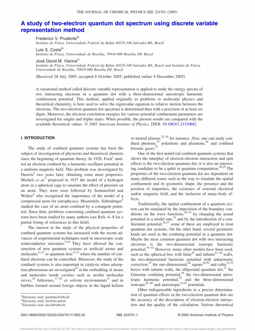
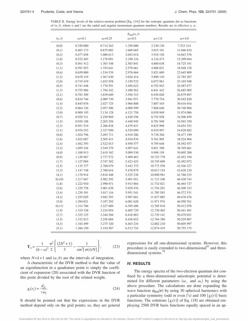
TABLE II. Energy levels of the relative-motion probof �n , l�, where n and l are the radial and angular mo

�n , l� �=0.1 �=0.25

�0,0� 0.350 000 0.714 262�0,1� 0.403 173 0.875 002�0,2� 0.477 658 1.080 613�1,0� 0.532 493 1.178 091�0,3� 0.561 412 1.303 348�1,1� 0.591 953 1.354 641�0,4� 0.650 000 1.534 539�1,2� 0.670 119 1.567 630�2,0� 0.719 419 1.652 938�0,5� 0.741 448 1.770 591�1,3� 0.755 984 1.794 242�2,1� 0.783 389 1.839 649�0,6� 0.834 744 2.009 730�1,4� 0.845 876 2.027 725�2,2� 0.864 126 2.057 506�3,0� 0.909 195 2.134 128�0,7� 0.929 311 2.250 969�1,5� 0.938 188 2.265 256�2,3� 0.951 519 2.286 838�3,1� 0.976 552 2.327 950�0,8� 1.024 796 2.493 711�1,6� 1.032 087 2.505 411�2,4� 1.042 393 2.522 013�3,2� 1.059 194 2.549 279�4,0� 1.100 913 2.619 342�0,9� 1.120 967 2.737 572�1,7� 1.127 094 2.747 382�2,5� 1.135 377 2.760 679�3,3� 1.147 748 2.780 634�4,1� 1.170 914 2.818 448�0,10� 1.217 667 2.982 292�1,8� 1.222 910 2.990 671�2,6� 1.229 758 3.001 639�3,4� 1.239 391 3.017 116�4,2� 1.255 029 3.042 393�5,0� 1.294 021 3.107 292�0,11� 1.314 786 3.227 689�1,9� 1.319 338 3.234 954�2,7� 1.325 125 3.244 204�3,5� 1.332 913 3.256 684�4,3� 1.344 499 3.275 320�5,1� 1.366 150 3.310 507

method depend only on the grid points; so, they are general

ownloaded 09 Sep 2013 to 200.130.19.138. This article is copyrighted as indicated in the abstract.

expressions for all one-dimensional systems. However, thisprocedure is easily extended to two-dimensional83 and three-dimensional systems.78

IV. RESULTS

The energy spectra of the two-electron quantum dot con-fined by a three-dimensional anisotropic potential is deter-mined for different parameters ��� and �z� by using theabove procedure. The calculations are done expanding thewave function �RM�r� by using 30 spherical harmonics witha particular symmetry �odd or even l’s� and 100 ��i�r�� basisfunctions. The solutions ��i�r�� of Eq. �18� are obtained em-

Eq. �14�� for the isotropic quantum dot as functionstum quantum numbers. Results are in effective a. u.

ERM�n , l��=0.5 �=1.0 �=4.0

.250 000 2.230 120 7.523 214

.609 665 3.015 101 11.046 810

.043 614 3.918 156 14.843 576

.190 116 4.134 473 15.299 044

.503 841 4.860 638 18.725 341

.578 661 4.968 821 18.948 128

.976 664 5.821 609 22.645 809

.024 414 5.890 110 22.785 207

.150 532 6.073 961 23.165 948

.456 622 6.792 943 26.587 677

.490 563 6.841 442 26.685 905

.556 315 6.936 020 26.879 897

.941 071 7.770 754 30.542 820

.966 808 7.807 445 30.616 916

.009 599 7.868 640 30.740 968

.121 758 8.030 949 31.074 086

.428 556 8.752 928 34.506 859

.448 945 8.781 948 34.565 350

.479 831 8.825 998 34.654 352

.539 099 8.910 997 34.828 682

.918 206 9.738 204 38.477 199

.934 876 9.761 905 38.524 904

.958 577 9.795 648 38.592 937

.997 641 9.851 398 38.705 661

.099 530 9.998 159 39.005 200

.409 463 10.725 778 42.452 194

.423 423 10.745 609 42.492 072

.442 375 10.772 558 42.546 327

.470 879 10.813 154 42.628 210

.525 238 10.890 981 42.788 235

.901 951 11.715 108 46.430 743

.913 864 11.732 021 46.464 727

.929 476 11.754 201 46.509 333

.951 541 11.785 583 46.572 531

.987 681 11.837 085 46.676 476

.081 628 11.971 974 46.950 761

.395 406 12.705 818 50.412 078

.405 729 12.720 465 50.441 491

.418 883 12.739 141 50.479 021

.436 652 12.764 389 50.529 807

.463 234 12.802 210 50.605 997

.513 724 12.874 435 50.755 175

lem �men

112222233333334444444444555555555556666666

ploying 2500 DVR basis functions equally spaced in an ap-

Reuse of AIP content is subject to the terms at: http://jcp.aip.org/about/rights_and_permissions

224701-5 Spectrum of two-electron quantum dot spectrum J. Chem. Phys. 123, 224701 �2005�

D

propriate interval for each pair of parameters �� and �z.These intervals are shown in Table I. Thus, the energy spec-tra presented here have a good precision of at least six sig-nificant digits. In Sec. IV A the isotropic situation ���=�z�is analyzed, while the anisotropic one �����z� is shown inSec. IV B.

A. Isotropic case

Initially the relative-motion eigenenergies �ERM� are cal-culated by using the procedure described above for the fol-lowing quantum dot parameters: ��=�z��=0.1, 0.25, 0.5,1.0, and 4.0. Due to the isotropy of the confinement poten-tial, results can be labeled using n and l, the radial and an-gular momentum quantum numbers, respectively. This hap-pens because the coupling term between different l’s in Eq.�15� disappears due to ��=0 when ��=�z. Then, in suchcase, n and l are the quantum numbers associated with therelative-motion problem.

The first 42 relative-motion energy levels for each caseare presented in Table II, where we can see some band struc-tures in the results for larger values of �. In each band, the nand l quantum numbers are related as follows: 2n+ l= p , pbeing an integer number. For example, the energy values ofthe states �n , l�= �0,4�, �1,2�, and �2,0� are very close for �=1.0 and 4.0, and they have p=4. As we will point out later,this represents that the influence of the electron-electron in-teraction is smaller for the strong confinement than for theweak confinement.

On the other hand, to calculate the total energies �E� wedo need to calculate the center-of-mass eigenenergies �ECM�.In the isotropic case, expression �11� is reduced to

ECM = �2N + L + 32�� , �25�

where N and L denote, respectively, the radial and angularmomentum quantum numbers related with the CM motion.Then, the complete spectrum �E=ECM+ERM� of the two-electron quantum dot confined by a three-dimensional isotro-pic harmonic potential can be determined from the results inTable II and Eq. �25�. It is important to point out that RMand CM quantum states which are 2l+1 and 2L+1 degener-

TABLE III. Three-dimensional two-electron quantum dot energies for selec

� �N ,L ,n , l� HF-1/Na HF-numb KS-1/Nc

0.25 �0,0,0,0� 1.1163 1.1241 1.16441.0 �0,0,0,0� 3.7673 3.7717 3.8711

�0,0,0,1��0,0,0,2��0,0,0,3��0,0,0,4�

4.0 �0,0,0,0� 13.5693 13.5693 13.7902

aHartree-Fock solutions by using the shifted 1/N method �Ref. 60�.bHartree-Fock solutions by using the accurate numerical technique �Ref. 60cKohn-Sham solutions by using the shifted 1/N method �Ref. 60�.dKohn-Sham solutions by using the accurate numerical technique �Ref. 60�.eExact Schrödinger solutions by using the shifted 1/N method �Ref. 60�.fExact Schrödinger solutions by using the accurate numerical technique �RegExact Schrödinger solutions by using the orbital integration method �Ref. 5hPresent results by using the discrete variable representation method.

ate with respect to the values of m and M, respectively.

ownloaded 09 Sep 2013 to 200.130.19.138. This article is copyrighted as indicated in the abstract.

The values of E for a small set of �N ,L ,n , l� states arepresented in Table III in order to compare with the onesobtained previously in Refs. 59 and 60. These total energiesof the two-electron quantum dot are determined in Ref. 60solving the Hartree-Fock �HF�, Kohn-Sham �KS�, andSchrödinger �exact� equations by using the shifted,1 /N �1/N� �Ref. 84� and Schwartz numeric85 �num� meth-ods, while in Ref. 59 the ones are calculated by using theorbital integration method �OIM�.86 A comparison betweenthe results shown in Table III indicates that the procedurebased on the DVR method gives results with a great preci-sion, and that the use of methodologies that compute com-pletely the correlation effects is very important.

es of the confinement parameter �. Energies are in effective a.u.

numd Exact-1 /Ne Exact-numf OIMg DVRh

742 1.0858 1.08926 1.089 262791 3.7217 3.73012 3.9632 3.730 120

4.7167 4.515 1015.5867 5.418 1566.5075 6.360 6387.4532 7.321 609

7928 13.5057 13.5232 13.523 214

�.

FIG. 1. Relative spectrum of isotropic two-electron quantum dot with re-spect to the confinement parameter �EN,L,n,l /�� for five �’s �0.1, 0.25, 0.5,

t valu

KS-

1.13.8

13.

�.

f. 609�.

1.0, and 4.0� and for the noninteracting �WI� case.

Reuse of AIP content is subject to the terms at: http://jcp.aip.org/about/rights_and_permissions

224701-6 Prudente, Costa, and Vianna J. Chem. Phys. 123, 224701 �2005�

D

Moreover, the spectrum with the lowest 245 energies of�N ,L ,n , l� states relative to the quantum dot parameter �i.e.,E /�� are displayed in Fig. 1 for five different �’s and fornoninteracting electron problem �i.e., solutions of Eq. �3�where HRM is written without the 1/r term�. In the last case,relative-motion eigenenergies satisfy a similar expression ofECM �Eq. �25��; i.e., ERM= �2n+ l+ 3

2��. In this figure, the

band structure appears clearly for ��0.5, and when the val-ues of the quantum dot parameter increase, the bands gosharpening and the interacting two-electron spectrum movestoward the noninteracting ones. However, for a weak con-finement ��→0� it is observed that a spectrum diffusesmore. Since the energy gaps that occur between the �N+2L+n+2l+3�-fold degenerate states of the noninteracting two-electron quantum dot �QD� is due to the spectrum associatedwith two harmonic oscillators, Fig. 1 indicates that for stron-ger QD parameters �larger values of �� the motion of theelectrons is mainly governed by the confinement potential,while for a weak confinement the electron-electron interac-tion plays an important and essential role.

In order to investigate this characteristic of the two-electron quantum dot, considered now are the relative-motion singlet states, i.e., solutions of Eq. �14� with oddvalues of the parameter l. For this purpose, in Fig. 2 aredisplayed the relative differences between the energy levelsof the interacting and noninteracting systems ��E�n,l�

rel

= �E�n,l�int −E�n,l�

non � /E�n,l�int � as a function of the �n , l� state. We can

see in Fig. 2 that the error in the electron-electron interactionis clearly larger for the weak confinements than for thestrong ones. For example, �E�0,0�

rel for �=0.1 is approxi-mately three times its value for �=4.0, while for �E�0,8�

rel thisdifference is about six times. Another interesting aspect thatcan be pointed out is that the larger the angular quantumnumber l’s, the smaller is the value of �E�n,l�

rel when it iscompared with the same band of energy levels. Moreover,the effect of the electron-electron interaction is larger in thelow-lying states than in the highly excited ones. This issuecan be explained if we call attention to the values of �E�0,l�

rel

rel

FIG. 2. Relative difference between the relative-motion singlet energy lev-els of the interacting and noninteracting isotropic two-electron quantum dotsystems as a function of the �n , l� state for five different confinement param-eters ��=0.1, 0.25, 0.5, 1.0, and 4.0�

and �E�n,0� when l and n are increased for all calculated �’s.

ownloaded 09 Sep 2013 to 200.130.19.138. This article is copyrighted as indicated in the abstract.

The discrete energy-level spacing55 �ELS� relative to���Ei

ELS/�= �Ei+1−Ei� /�� as a function of relative energy�Ei /�� for singlets is shown in Fig. 3 for interacting systemswith �=0.1, 0.25, 0.5, 0.1, and 4.0 for the noninteractingtwo-electron one. This figure supplies some informationabout the energy gaps that appear at the energy spectrum.The first is that energy gaps that occur in the noninteractingsystem are due to the spectrum of the harmonic oscillator.The second is that the energy gap decreases, and the degen-eracies are lifted when the electron-electron interaction isincluded in the model. However, the intensities of these ef-fects depend clearly on the quantum dot parameter �. Theyare more obvious for the weak than for the strong confine-ment. Therefore, a repeated stretching phase of the energygaps is observed for the interacting isotropic two-electronquantum dot. Note that a similar discussion was done fortwo-electron anisotropic two-dimensional quantum dots inRef. 55.

B. Anisotropic case

The relative-motion eigenenergies �ERM� associated with

FIG. 3. Discrete relative-motion singlet energy-level spacing �ELS� for theisotropic two-electron quantum dot relative to � as a function of relativeenergy for �a� �=0.1, �b� �=0.25, �c� �=0.5, �d� �=1.0, �e� �=4.0, and �f�noninteracting system.

�n ,m ,nz� states are calculated for the following quantum dot

Reuse of AIP content is subject to the terms at: http://jcp.aip.org/about/rights_and_permissions

224701-7 Spectrum of two-electron quantum dot spectrum J. Chem. Phys. 123, 224701 �2005�

D

parameters: �z=0.1, 0.25, 0.5, 1.0, and 4.0 with ��=0.5.The first 42 relative-motion energy levels for each pair of �z

and �� are presented in Table IV. They are also shown inFig. 4 together with the noninteracting energy levels, whichare given by ERM

non = �2n+m+1���+ �nz+0.5��z.Some interesting information can be observed in Table

IV and Fig. 4. The first one is the existence of a band struc-ture in energy levels when the electron-electron interaction isconsidered, while to the noninteracting ones there is a regu-lar structure. However, different from the isotropic case, theelectronic states in these bands do not present a general rule.The second consideration is that the error obtained to calcu-late the noninteracting triplet ground state is smaller than the

TABLE IV. Energy levels of the relative-motion problem �Eq. �14�� for the aby �n ,m ,nz�, where n and m are the radial and the azimuthal quantum nunumber associated with the z-direction harmonic oscillator. Results are in e

�z=0.1 �z=0.25 �

�0,0,0� 0.827 006 �0,0,0� 1.046 978 �0,0,0��0,0,1� 0.836 407 �0,0,1� 1.156 472 �0,1,0��0,0,2� 0.981 087 �0,0,2� 1.410 785 �0,0,1��0,0,3� 1.013 310 �0,1,0� 1.452 050 �0,2,0��0,0,4� 1.138 679 �0,0,3� 1.610 223 �0,1,1��0,0,5� 1.196 519 �0,1,1� 1.620 164 �0,0,2��0,1,0� 1.301 681 �0,0,4� 1.843 295 �1,0,0��0,0,6� 1.308 638 �0,1,2� 1.852 083 �0,3,0��0,1,1� 1.324 935 �0,2,0� 1.899 628 �0,2,1��0,0,7� 1.383 900 �1,0,0� 1.981 385 �0,1,0��0,1,2� 1.437 930 �0,0,5� 2.073 775 �0,0,3��0,0,8� 1.488 817 �0,1,3� 2.078 237 �1,1,0��0,1,3� 1.499 648 �0,2,1� 2.094 963 �1,0,1��0,0,9� 1.574 036 �1,0,1� 2.118 335 �0,4,0��0,1,4� 1.600 217 �0,0,6� 2.310 391 �0,3,1��0,0,10� 1.674 289 �0,1,4� 2.313 589 �0,2,2��0,1,5� 1.682 564 �0,2,2� 2.325 521 �0,1,3��0,0,11� 1.765 731 �0,3,0� 2.366 007 �0,0,4��0,2,0� 1.778 543 �1,0,2� 2.380 097 �1,2,0��0,1,6� 1.780 066 �1,1,0� 2.415 529 �1,1,1��1,0,0� 1.800 018 �0,0,7� 2.548 835 �1,0,2��0,2,1� 1.815 194 �0,1,5� 2.551 034 �2,0,0��1,0,1� 1.819 182 �0,2,3� 2.558 612 �0,5,0��0,0,12� 1.864 647 �0,3,1� 2.576 212 �0,4,1��0,1,7� 1.870 419 �1,0,3� 2.587 256 �0,3,2��0,2,2� 1.913 623 �1,1,1� 2.594 909 �0,2,3��1,0,2� 1.947 750 �0,0,8� 2.789 338 �0,1,4��0,0,13� 1.958 698 �0,1,6� 2.790 976 �0,0,5��0,1,8� 1.967 359 �0,2,4� 2.796 466 �1,3,0��0,2,3� 1.989 525 �0,3,2� 2.808 464 �1,2,1��1,0,3� 1.995 911 �1,0,4� 2.826 095 �1,1,2�

�0,0,14� 2.056 931 �1,1,2� 2.834 096 �1,0,3��0,1,9� 2.061 292 �0,4,0� 2.842 227 �2,1,0��0,2,4� 2.084 078 �1,2,0� 2.876 722 �2,0,1��1,0,4� 2.112 190 �2,0,0� 2.941 493 �0,6,0��0,0,15� 2.152 656 �0,0,9� 3.031 189 �0,5,1��0,1,10� 2.158 130 �0,1,7� 3.032 434 �0,4,2��0,2,5� 2.173 173 �0,2,5� 3.036 507 �0,3,3��1,0,5� 2.180 899 �0,3,3� 3.044 758 �0,2,4��0,0,16� 2.250 653 �1,0,5� 3.059 424 �0,1,5��0,1,11� 2.253 980 �0,4,1� 3.061 570 �0,0,6��0,3,0� 2.259 337 �1,1,3� 3.063 223 �1,4,0�

one obtained to calculate the noninteracting singlet ground

ownloaded 09 Sep 2013 to 200.130.19.138. This article is copyrighted as indicated in the abstract.

state. This indicates that the electron-electron interaction ismore important for singlet states than for triplet ones. Similarconclusions were observed when we compare the resultsfrom Hartree-Fock and from the exact treatment for this sys-tem in Ref. 63. Moreover, some degeneracies between stateswith the same quantum number m but with different quantumnumbers l and nz can be seen for �z=1.0 in Table IV. Forexample, the states �0, m, 1� and �1, m, 0� have the sameenergy within the results’ precision.

In order to analyze the degeneracies that happen in theenergy spectrum, the total-energy levels associated with�N ,M ,NZ ,n ,m ,nz� states with up to two excitations for dif-ferent �z’s are shown in Table V. Some selected states from

opic quantum dot for five �z parameters and ��=0.5. The states are labeleds associated with the planar oscillator, respectively, and nz is the quantumve a.u.

�z=1.0 �z=4.0

.250 000 �0,0,0� 1.553 151 �0,0,0� 3.114 320

.609 665 �0,1,0� 1.880 816 �0,1,0� 3.402 864

.609 665 �0,2,0� 2.305 474 �0,2,0� 3.816 901

.043 614 �1,0,0� 2.434 862 �1,0,0� 4.005 659

.043 614 �0,0,1� 2.434 888 �0,3,0� 4.268 765

.043 614 �0,3,0� 2.761 631 �1,1,0� 4.357 902

.190 116 �0,1,1� 2.833 564 �0,4,0� 4.737 222

.503 841 �1,1,0� 2.833 591 �1,2,0� 4.791 919

.503 841 �0,4,0� 3.232 266 �2,0,0� 4.937 499

.503 841 �1,2,0� 3.279 371 �0,5,0� 5.214 582

.503 841 �0,2,1� 3.279 371 �1,3,0� 5.252 508

.578 661 �2,0,0� 3.332 921 �2,1,0� 5.327 003

.578 661 �1,0,1� 3.332 951 �0,6,0� 5.697 342

.976 664 �0,0,2� 3.446 825 �1,4,0� 5.725 610

.976 664 �0,5,0� 3.710 894 �2,2,0� 5.773 209

.976 664 �0,3,1� 3.744 716 �3,0,0� 5.891 017

.976 664 �1,3,0� 3.744 716 �0,7,0� 6.183 659

.976 664 �1,1,1� 3.787 061 �1,5,0� 6.205 771

.024 414 �2,1,0� 3.787 073 �2,3,0� 6.239 627

.024 414 �0,1,2� 3.824 802 �3,1,0� 6.303 980

.024 414 �0,6,0� 4.194 465 �0,8,0� 6.672 462

.150 532 �1,4,0� 4.220 232 �1,6,0� 6.690 367

.456 622 �0,4,1� 4.220 232 �2,4,0� 6.716 048

.456 622 �2,2,0� 4.252 508 �3,2,0� 6.758 419

.456 622 �1,2,1� 4.252 508 �4,0,0� 6.857 057

.456 622 �0,2,2� 4.270 123 �0,0,1� 7.052 214

.456 622 �3,0,0� 4.275 896 �0,9,0� 7.163 082

.456 622 �2,0,1� 4.275 907 �1,7,0� 7.177 963

.490 563 �1,0,2� 4.376 978 �2,5,0� 7.198 310

.490 563 �0,0,3� 4.377 045 �3,3,0� 7.229 035

.490 563 �0,7,0� 4.681 335 �4,1,0� 7.285 899

.490 563 �1,5,0� 4.701 795 �0,1,1� 7.383 965

.556 315 �0,5,1� 4.701 795 �0,10,0� 7.655 077

.556 315 �1,3,1� 4.727 023 �1,8,0� 7.667 699

.941 071 �2,3,0� 4.727 023 �2,6,0� 7.684 336

.941 071 �0,3,2� 4.736 841 �3,4,0� 7.707 958

.941 071 �2,1,1� 4.751 629 �4,2,0� 7.746 288

.941 071 �3,1,0� 4.751 632 �0,2,1� 7.807 897

.941 071 �0,1,3� 4.796 416 �5,0,0� 7.830 906

.941 071 �1,1,2� 4.796 492 �1,0,1� 7.931 877

.941 071 �0,8,0� 5.170 536 �1,9,0� 8.159 022

.966 808 �1,6,0� 5.187 284 �2,7,0� 8.172 956

nisotrmberffecti

z=0.5

111222222222222222333333333333333333333333

this table are displayed in Fig. 5 as functions of the �z pa-

Reuse of AIP content is subject to the terms at: http://jcp.aip.org/about/rights_and_permissions

224701-8 Prudente, Costa, and Vianna J. Chem. Phys. 123, 224701 �2005�

D

rameter. In such case the total energy is the addition of therelative-motion energy, shown in Table IV, with the center-of-mass energy given by Eq. �11�. We can see a splitting onthe degenerate total-energy levels for ��=�z=0.5 when �z

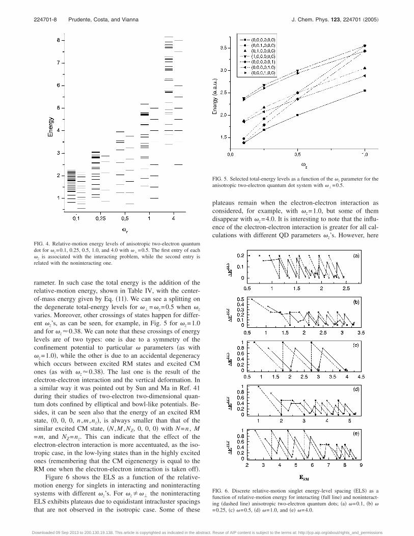
varies. Moreover, other crossings of states happen for differ-ent �z’s, as can be seen, for example, in Fig. 5 for �z=1.0and for �z�0.38. We can note that these crossings of energylevels are of two types: one is due to a symmetry of theconfinement potential to particular � parameters �as with�z=1.0�, while the other is due to an accidental degeneracywhich occurs between excited RM states and excited CMones �as with �z�0.38�. The last one is the result of theelectron-electron interaction and the vertical deformation. Ina similar way it was pointed out by Sun and Ma in Ref. 41during their studies of two-electron two-dimensional quan-tum dots confined by elliptical and bowl-like potentials. Be-sides, it can be seen also that the energy of an excited RMstate, �0, 0, 0, n ,m ,nz�, is always smaller than that of thesimilar excited CM state, �N ,M ,NZ, 0, 0, 0� with N=n , M=m, and NZ=nz. This can indicate that the effect of theelectron-electron interaction is more accentuated, as the iso-tropic case, in the low-lying states than in the highly excitedones �remembering that the CM eigenenergy is equal to theRM one when the electron-electron interaction is taken off�.

Figure 6 shows the ELS as a function of the relative-motion energy for singlets in interacting and noninteractingsystems with different �z’s. For �z��� the noninteractingELS exhibits plateaus due to equidistant intracluster spacings

FIG. 4. Relative-motion energy levels of anisotropic two-electron quantumdot for �z=0.1, 0.25, 0.5, 1.0, and 4.0 with ��=0.5. The first entry of each�z is associated with the interacting problem, while the second entry isrelated with the noninteracting one.

that are not observed in the isotropic case. Some of these

ownloaded 09 Sep 2013 to 200.130.19.138. This article is copyrighted as indicated in the abstract.

plateaus remain when the electron-electron interaction asconsidered, for example, with �z=1.0, but some of themdisappear with �z=4.0. It is interesting to note that the influ-ence of the electron-electron interaction is greater for all cal-culations with different QD parameters �z’s. However, here

FIG. 5. Selected total-energy levels as a function of the �z parameter for theanisotropic two-electron quantum dot system with ��=0.5.

FIG. 6. Discrete relative-motion singlet energy-level spacing �ELS� as afunction of relative-motion energy for interacting �full line� and noninteract-ing �dashed line� anisotropic two-electron quantum dots; �a� �=0.1, �b� �

=0.25, �c� �=0.5, �d� �=1.0, and �e� �=4.0.

Reuse of AIP content is subject to the terms at: http://jcp.aip.org/about/rights_and_permissions

0.5, 1.0, and 4.0 with ��=0.5.

224701-9 Spectrum of two-electron quantum dot spectrum J. Chem. Phys. 123, 224701 �2005�

Downloaded 09 Sep 2013 to 200.130.19.138. This article is copyrighted as indicated in the abstract.

are also observed behaviors that are similar to the isotropicsituation. We can also note some energy gaps on the spec-trum for noninteracting systems, and the reduction of theenergy gaps and the break of the degeneracy when the inter-action is considered in the model. This confirms the analysisin Ref. 55 for two-dimensional quantum dots that theelectron-electron interaction changes the behavior of the ELSfunction significantly, and the preservation of this featureoccurs only for the situation when it is compared with thenoninteracting situation.

Finally, the spectrum of the two-electron anisotropicthree-dimensional quantum dot to �z=0.1, 0.25, 0.5, 1.0, and4.0 with ��=0.5 is displayed in Fig. 7. The band structuresare observed for all �’s, but they appear more clearly for�z�0.5. This indicates again that the motion of electrons ismainly governed by the confinement potential for strong QDparameters. In the anisotropic case, however, it cannot estab-lish a general relation to the occurrence of degenerate states.

V. CONCLUSION

In this paper we have studied theoretically a two-electron quantum dot using a three-dimensional anisotropicharmonic confinement potential. In particular, we focus onthe effect of the electron-electron interaction and the aniso-tropy on the ground and excited electronic states of the sys-

e anisotropic two-electron quantum dot as functionsm numbers associated with the CM problem androblem. Results are in effective a.u.

�z=0.5 �z=1.0 �z=4.0

�a� 2.000 000 �a� 2.553 151 �a� 5.614 320�b� 2.359 665 �b� 2.880 816 �b� 5.902 864�c� 2.359 665 �d� 3.053 151 �d� 6.114 320�d� 2.500 000 �h� 3.305 474 �h� 6.316 901�e� 2.500 000 �l� 3.380 816 �l� 6.402 864�f� 2.793 614 �m� 3.434 862 �m� 6.505 659�g� 2.793 614 �c� 3.434 888 �p� 6.614 320�h� 2.793 614 �p� 3.553 151 �q� 6.614 320�i� 2.859 665 �e� 3.553 151 �s� 6.857 902�j� 2.859 665 �q� 3.553 151 �t� 6.902 864�k� 2.859 665 �g� 3.833 564 �w� 7.005 659�l� 2.859 665 �s� 3.833 591 �y� 7.114 320�m� 2.940 116 �k� 3.880 816 �z� 7.437 499�n� 3.000 000 �t� 3.880 816 �aa� 7.505 659�o� 3.000 000 �w� 3.934 862 �ab� 7.614 320�p� 3.000 000 �j� 3.934 888 �c� 9.552 214�q� 3.000 000 �o� 4.053 151 �e� 9.614 320�r� 3.328 661 �y� 4.053 151 �g� 9.883 965�s� 3.328 661 �z� 4.332 921 �k� 9.902 864�t� 3.359 665 �r� 4.332 951 �j�10.052 214�u� 3.359 665 �aa� 4.434 862 �o�10.114 320�v� 3.440 116 �v� 4.434 862 �r�10.431 877�w� 3.440 116 �i� 4.434 888 �v�10.505 659�x� 3.500 000 �u� 4.434 888 �u�10.552 214�y� 3.500 000 �f� 4.446 825 �x�10.614 320�z� 3.900 532 �n� 4.553 151 �f�13.527 801�aa� 3.940 116 �x� 4.553 151 �i�13.552 214�ab� 4.000 000 �ab� 4.553 151 �n�13.614 320

FIG. 7. Spectrum of anisotropic two-electron quantum dot for �z=0.1, 0.25,

TABLE V. Total-energy levels up to two excitations for thof �N ,M ,Nz ,n ,m ,nz�, where �N ,M ,Nz� are the quantu�n ,m ,nz� are the quantum ones associated with the RM p

� �z=0.1 �z=0.25

a �0,0,0,0,0,0� �a� 1.377 006 �a� 1.671 978b �0,0,0,0,1,0� �c� 1.386 407 �c� 1.781 472c �0,0,0,0,0,1� �e� 1.477 006 �e� 1.921 978d �0,1,0,0,0,0� �i� 1.486 407 �i� 2.031 472e �0,0,1,0,0,0� �f� 1.531 087 �f� 2.035 785f �0,0,0,0,0,2� �n� 1.577 006 �b� 2.077 050g �0,0,0,0,1,1� �b� 1.851 681 �n� 2.171 978h �0,0,0,0,2,0� �d� 1.877 006 �d� 2.171 978i �0,0,1,0,0,1� �g� 1.874 935 �g� 2.245 164j �0,1,0,0,0,1� �j� 1.886 407 �j� 2.281 472k �0,0,1,0,1,0� �k� 1.951 681 �k� 2.327 050l �0,1,0,0,1,0� �o� 1.977 006 �o� 2.421 978m �0,0,0,1,0,0� �h� 2.328 543 �h� 2.524 628n �0,0,2,0,0,0� �m� 2.350 018 �l� 2.577 050o �0,1,1,0,0,0� �l� 2.351 681 �m� 2.606 385p �0,2,0,0,0,0� �r� 2.369 182 �p� 2.671 978q �1,0,0,0,0,0� �p� 2.377 006 �q� 2.671 978r �0,0,0,1,0,1� �q� 2.377 006 �r� 2.743 335s �0,0,0,1,1,0� �u� 2.386 407 �u� 2.781 472t �1,0,0,0,1,0� �v� 2.450 018 �v� 2.856 385u �1,0,0,0,0,1� �x� 2.477 006 �x� 2.921 978v �0,0,1,1,0,0� �s� 2.830 019 �s� 3.040 529w �0,1,0,1,0,0� �w� 2.850 018 �t� 3.077 050x �1,0,1,0,0,0� �t� 2.851 681 �w� 3.106 385y �1,1,0,0,0,0� �y� 2.877 006 �y� 3.171 978z �0,0,0,2,0,0� �z� 3.330 333 �z� 3.566 493aa �1,0,0,1,0,0� �aa� 3.350 018 �aa� 3.606 385ab �2,0,0,0,0,0� �ab� 3.377 006 �ab� 3.671 978

tem. For this purpose, we have considered the isotropic ��1

Reuse of AIP content is subject to the terms at: http://jcp.aip.org/about/rights_and_permissions

224701-10 Prudente, Costa, and Vianna J. Chem. Phys. 123, 224701 �2005�

D

=�z� and anisotropic ��1��z� situations for different valuesof the QD parameters �� and �z. The spectra, consideringboth singlet and triplet states, have been computed using avariational approach based on the discrete variable represen-tation method. The DVR method has been widely applied inliterature to study problems in molecular and chemical phys-ics, and here it is used with spherical harmonics, for the firsttime, to solve the eigenvalue-eigenvector equation of therelative motion of the electrons in a three-dimensional quan-tum dot. The procedure has shown very accurate calculationswith at least six significant digits on the eigenvalues of en-ergy. It is important to point out that the DVR method con-siders completely the electron-electron interaction.

The present results are displayed in Fig. 1–7 and TablesI–V. The major conclusions are summarized as follows: �i�The effects of the electron-electron interaction are more im-portant for weak confinement potentials than for strong ones,for singlet states than for triplet states, and for low-lyingstates than for highly excited states. �ii� The degeneraciesthat exist in the noninteracting situation are lifted when theelectron-electron interaction is included. �iii� The existenceof vertical deformations breaking degeneracies that exist inthe isotropic quantum dots. Other state crossings can appearfor particular �� and �z parameters due to a combination ofthe electronic interaction and the vertical deformation. �iv�The observation of equidistant intracluster spacings of en-ergy levels in quantum dots with anisotropic potential. And�v� the results obtained using the DVR method, when com-pared with others previously published, perform with greatprecision. So it demonstrates that such a method can be ap-plied to the study of different confined quantum systems withconfidence.

Finally, we call attention to the relation between valuesof the QD parameters ��� and �z� which defines the con-finement intensity and the Coulombian interaction �see, forexample, Fig. 1 for the isotropic case and Fig. 4 for theanisotropic situation�. In this context it is interesting to notethat a strong confinement is associated with a high-electronicdensity, while a weak confinement is associated with a low-electronic density. Moreover, we have verified that theelectron-electron interaction is not so important for strongconfinements; then in such a case the interaction can betreated as a perturbation of the noninteracting QD system.However, this is not true in the case of low-electronic den-sity, and, in such a case, it is fundamental to employ or todevelop methodologies which compute completely theelectron-electron interaction like the one used in the presentpaper.

ACKNOWLEDGMENTS

One of us �F.V.P.� would like to thank Marcilio N.Guimarães and Marcos M. Almeida for useful discussions.This work has been supported by the Conselho Nacional deDesenvolvimento Científico e Tecnológico �CNPq-Brazil�.

1 V. Fock, Z. Phys. 47, 446 �1928�.2 C. G. Darwin, Proc. Cambridge Philos. Soc. 27, 86 �1930�.3 A. Michels, J. de Boer, and A. Bijl, Physica �Amsterdam� 4, 981 �1937�.4

A. Sommerfeld and H. Welker, Ann. Phys. 32, 56 �1938�.

ownloaded 09 Sep 2013 to 200.130.19.138. This article is copyrighted as indicated in the abstract.

5 E. Schrödinger, Proc. R. Ir. Acad., Sect. A 46, 183 �1941�.6 P. O. Fröman, S. Yngve, and N. Fröman, J. Math. Phys. 28, 1813 �1987�.7 W. Jaskólski, Phys. Rep. 271, 1 �1996�.8 J. P. Connerade, V. K. Dolmatov, and P. A. Laksbmit, J. Phys. B 33, 251�2000�.

9 L. Jacak, O. Hawrylak, and A. Wojs, Quantum Dots �Springer, New york1998�.

10 A. Zrenner, J. Chem. Phys. 112, 7790 �2000�.11 R. C. Ashoori, Nature �London� 379, 413 �1996�.12 T. H. Dosterkamp, T. Fujisawa, W. G. van der Wiel, K. Ishibashi, R. V.

Hijman, and L. P. Kouwenhoven, Nature �London� 395, 823 �1998�.13 N. F. Johnson, J. Phys.: Condens. Matter 7, 965 �1995�.14 S. Tarucha, D. G. Austing, T. Honda, R. T. van der Hage, and L. P.

Kouwenhoven, Phys. Rev. Lett. 77, 3613 �1996�.15 K. H. Frank, R. Didde, H. J. Sagner, and W. Eberhardt, Phys. Rev. B 39,

940 �1989�.16 Z. K. Tang, Y. Nozue, and T. J. Goto, J. Phys. Soc. Jpn. 61, 2943 �1992�.17 H. W. Kroto, J. R. Heath, S. C. O’Brian, R. F. Curl, and R. E. Smalley,

Nature �London� 318, 162 �1985�.18 I. Lazlo and L. Udvardi, Chem. Phys. Lett. 136, 418 �1987�.19 J. Cioslowski and E. D. Fleischmann, J. Chem. Phys. 94, 3730 �1991�.20 A. S. Baltenkov, J. Phys. B 32, 2745 �1999�.21 C. Reichardt, Solvents and Solvents Effects in Organic Chemistry �VCH,

Weinheim, 1988�.22 M. Takani, Comments At. Mol. Phys. 32, 219 �1996�.23 B. Saha, T. K. Mukherjee, P. K. Mukherjee, and G. H. F. Diercksen,

Theor. Chem. Acc. 108, 305 �2002�.24 P. K. Mukherjee, J. Karwowski, and G. H. F. Diercksen, Chem. Phys.

Lett. 363, 323 �2002�.25 M. Grinberg, W. Jaskólski, Cz. Koepke, J. Plannelles, and M. Janowicz,

Phys. Rev. B 50, 6504 �1994�.26 V. Gudmundson and R. R. Gerhardts, Phys. Rev. B 43, 12098 �1991�.27 M. Grossmann and M. Holthaus, Z. Phys. B: Condens. Matter 97, 319

�1995�.28 J. H. Jefferson, M. Fearn, and D. L. J. Tipton, Phys. Rev. A 66, 042328

�2002�.29 G. Tóth and C. S. Lent, Phys. Rev. A 63, 052315 �2001�.30 P. L. Goodfriend, J. Phys. B 23, 1373 �1990�.31 Y. P. Varshni, J. Phys. B 30, L589 �1997�.32 R. Rivelino and J. D. M. Vianna, J. Phys. B 34, L645 �2001�.33 C. F. Destefani, J. D. M. Vianna, and G. E. Marques, Semicond. Sci.

Technol. 19, L90 �2004�.34 M. N. Guimarães and F. V. Prudente, J. Phys. B 38, 2811 �2005�.35 C. Zicovich-Wilson, J. H. Planelles, and W. Jaskólski, Int. J. Quantum

Chem. 50, 429 �1994�.36 E. Ley-Koo and S. Rubinstein, J. Chem. Phys. 71, 351 �1979�.37 L. S. Costa, F. V. Prudente, P. H. Acioli, J. J. Soares Neto, and J. D. M.

Vianna, J. Phys. B 32, 2461 �1999�.38 U. Merkt, J. Huser, and M. Wagner, Phys. Rev. B 43, 7320 �1991�.39 M. Macucci, K. Hess, and G. J. Iafrate, Phys. Rev. B 48, R4879 �1997�.40 C. Yannouleas and U. Landman, Phys. Rev. Lett. 85, 1726 �2000�.41 L. L. Sun and F. C. Ma, J. Appl. Phys. 94, 5844 �2003�.42 S. Bednarek, B. Szafran, and J. Adamowski, Phys. Rev. B 59, 13036

�1999�.43 D. C. Thompson and A. Alavi, Phys. Rev. B 66, 235118 �2002�.44 J. Jung and J. E. Alvarellos, J. Chem. Phys. 118, 10825 �2003�.45 J. Jung, P. García-González, J. E. Alvarellos, and R. W. Godby, Phys.

Rev. A 69, 052501 �2004�.46 D. C. Thompson and A. Alavi, J. Chem. Phys. 122, 124107 �2005�.47 D. Pfannkuche and R. R. Gerhardts, Phys. Rev. B 44, 13132 �1991�.48 E. A. Salter, G. W. Trucks, and D. S. Cyphert, Am. J. Phys. 69, 120

�2001�.49 G. W. Bryant, Phys. Rev. Lett. 59, 1140 �1987�.50 E. Räsänen, A. Harju, M. J. Puska, and R. M. Nieminen, Phys. Rev. B

69, 165309 �2004�.51 A. Alavi, J. Chem. Phys. 113, 7735 �2000�.52 D. M. Mitnik, Phys. Rev. A 70, 022703 �2004�.53 G. Cantele, D. Ninno, and G. Iadonisi, Phys. Rev. B 64, 125325 �2001�.54 J. Adamowski, M. Sobkowicz, B. Szafran, and S. Bednarek, Phys. Rev. B

62, 4234 �2000�.55 P. S. Drouvelis, P. Schmelcher, and F. K. Diakonos, Phys. Rev. B 69,

035333 �2004�.56 N. R. Kestner and O. Sinanoglu, Phys. Rev. 128, 2687 �1962�.57

J. Cioslowski and K. Pernal, J. Chem. Phys. 113, 8434 �2000�.

Reuse of AIP content is subject to the terms at: http://jcp.aip.org/about/rights_and_permissions

224701-11 Spectrum of two-electron quantum dot spectrum J. Chem. Phys. 123, 224701 �2005�

D

58 P. M. Laufer and J. B. Krieger, Phys. Rev. A 33, 1480 �1986�.59 W. C. Lee and T. K. Lee, J. Phys.: Condens. Matter 14, 1045 �2002�.60 R. Pino and V. M. Villalba, J. Phys.: Condens. Matter 13, 11651 �2001�.61 T. Sako and G. H. F. Diercksen, J. Phys.: Condens. Matter 15, 5487

�2003�.62 J. T. Lin and T. F. Jiang, Phys. Rev. B 64, 195323 �2001�.63 D. Pfannkuche, V. Gudmundsson, and P. A. Maksym, Phys. Rev. B 47,

2244 �1993�.64 C. E. Creffield, J. H. Jefferson, S. Sarkar, and D. L. J. Tipton, Phys. Rev.

B 62, 7249 �2000�.65 S. Kais, D. R. Herschbach, N. C. Handy, C. W. Murray, and G. J. Lam-

ing, J. Chem. Phys. 99, 417 �1993�.66 B. Szafran, S. Bednarek, J. Adamowski, M. B. Tavernier, E. Anisimovas,

and F. M. Peeters, Eur. Phys. J. D 28, 373 �2004�.67 T. F. Jiang, X. Tong, and S. Chu, Phys. Rev. B 63, 045317 �2001�.68 M. Wagner, U. Merkt, and A. V. Chaplik, Phys. Rev. B 45, 1951 �1992�.69 G. Cipriani, M. Rosa-Clot, and S. Taddei, Phys. Rev. B 61, 7536 �2000�.70 A. Harju, V. A. Sverdlov, R. M. Nieminen, and V. Halonen, Phys. Rev. B

59, 5622 �1999�.71 J. Harting, O. Mülken, and P. Borrmann, Phys. Rev. B 62, 10207 �2000�.72 M. Taut, Phys. Rev. A 48, 3561 �1993�.73 M. Dineykhan and R. G. Nazmitdinov, Phys. Rev. B 55, 13707 �1997�.

ownloaded 09 Sep 2013 to 200.130.19.138. This article is copyrighted as indicated in the abstract.

74 S. Kais, D. R. Herschbach, and R. D. Levine, J. Chem. Phys. 91, 7791�1989�.

75 S. Klama and E. G. Mishchenko, J. Phys.: Condens. Matter 10, 3411�1998�.

76 L. Serra, R. G. Nazmitdinov, and A. Puente, Phys. Rev. B 68, 035341�2003�.

77 T. Sako and G. H. F. Diercksen, J. Phys. B 36, 1681 �2003�.78 J. C. Light and T. Carrington, Jr., Adv. Chem. Phys. 114, 263 �2000�.79 F. V. Prudente, A. Riganelli, and A. J. C. Varandas, Rev. Mex. Fis. 47,

568 �2001�.80 R. G. Littlejohn, M. Cargo, T. Carrington, Jr., K. A. Mitchell, and B.

Poirier, J. Chem. Phys. 116, 8691 �2002�.81 J. T. Muckerman, Chem. Phys. Lett. 173, 200 �1990�.82 D. T. Colbert and W. H. Miller, J. Chem. Phys. 96, 1982 �1992�.83 F. V. Prudente, L. S. Costa, and J. J. Soares Neto, J. Mol. Struct.:

THEOCHEM 394, 169 �1997�.84 T. Imbo, A. Pagnamenta, and U. Sukhatme, Phys. Rev. D 29, 1669

�1984�.85 C. Schwartz, J. Math. Phys. 26, 411 �1985�.86 R. Friedberg, T. D. Lee, and W. Q. Zhao, Nuovo Cimento Soc. Ital. Fis.,

A 112A, 1195 �1999�.

Reuse of AIP content is subject to the terms at: http://jcp.aip.org/about/rights_and_permissions