
A Study of Riordan Arrays with Applications to Continued Fractions, Orthogonal Polynomials and
259
A Study of Riordan Arrays with Applications to Continued Fractions, Orthogonal Polynomials and Lattice Paths by Aoife Hennessy A thesis submitted in partial fulfillment for the degree of Doctor of Philosophy in the Department of Computing, Mathematics and Physics Waterford Institute of Technology Supervisor: Dr. Paul Barry Head of the School of Science Waterford Institute of Technology October 2011
Transcript of A Study of Riordan Arrays with Applications to Continued Fractions, Orthogonal Polynomials and

A Study of Riordan Arrayswith Applications to Continued Fractions,Orthogonal Polynomials and Lattice Paths
by
Aoife Hennessy
A thesis submitted in partial fulfillment for thedegree of Doctor of Philosophy
in the
Department of Computing, Mathematics and PhysicsWaterford Institute of Technology
Supervisor: Dr. Paul BarryHead of the School of Science
Waterford Institute of Technology
October 2011

1
Declaration of Authorship
I, AOIFE HENNESSY, declare that this thesis titled, ‘A Study of Riordan Arrays withApplications to Continued Fractions, Orthogonal Polynomials and Lattice Paths’ andthe work presented in it are my own. I confirm that:
1. This work was done wholly or mainly while in candidature for a research degreeat this Institute.
2. Where I have consulted the published work of others, this is always clearly at-tributed.
3. Where I have quoted from the work of others, the source is always given. Withthe exception of such quotations, this thesis is entirely my own work.
4. I have acknowledged all main sources of help.
Signed:
Date:

Abstract
We study integer sequences using methods from the theory of continued fractions, or-thogonal polynomials and most importantly from the Riordan groups of matrices, theordinary Riordan group and the exponential Riordan group. Firstly, we will intro-duce the Riordan group and their links through orthogonal polynomials to the Stieltjesmatrix. Through the context of Riordan arrays we study the classical orthogonalpolynomials, the Chebyshev polynomials. We use Riordan arrays to calculate determi-nants of Hankel and Toeplitz-plus-Hankel matrices, extending known results relatingto the Chebyshev polynomials of the third kind to the other members of the family ofChebyshev polynomials. We then define the form of the Stieltjes matrices of importantsubgroups of the Riordan group. In the following few chapters, we develop the well es-tablished links between orthogonal polynomials, continued fractions and Motzkin pathsthrough the medium of the Riordan group. Inspired by these links, we extend resultsto the Lukasiewicz paths, and establish relationships between Motzkin, Schroder andcertain Lukasiewicz paths. We concern ourselves with the Binomial transform of inte-ger sequences that arise from the study of Lukasiewicz and Motzkin paths and we alsostudy the effects of this transform on lattice paths. In the latter chapters, we applythe Riordan array concept to the study of sequences related to MIMO communica-tions through integer arrays relating to the Narayana numbers. In the final chapter,we use the exponential Riordan group to study the historical Euler-Seidel matrix. Wecalculate the Hankel transform of many families of sequences encountered throughout.

1
Acknowledgements
I wish to express my most sincere gratitude to Dr. Paul Barry, who has been extremelyhelpful and patient. It has been a privilege to work with Paul over the last few years.I could not have wished for a better supervisor.
To Peter, thank you for cooking for me, keeping me in wine, and putting up with meplaying on my laptop for an unforgivable length of time!
Lastly, thanks to my family and friends for all their support, especially Mam, Keith,and all my mothering Aunties, whose kindness I can only hope to return.

2
Notation
• R The set of real numbers.
• Z The set of integers.
• Z2 The integer lattice.
• Q The set of rational numbers.
• C The set of complex numbers.
• o.g.f . Ordinary generating function.
• e.g.f . Exponential generating function.
• c(x) The generating function of the sequence of Catalan numbers.
• cn The nth Catalan number.
• [xn]f(x) The coefficient of the xn term of the power series f(x).
• 0n The sequence 1, 0, 0, 0, . . . , with o.g.f. 1.
• f(x) or Rev(f(x)) The series reversion of the series f(x), where f(0) = 0.
• L A Riordan array.
• L The matrix with Ln,k = Ln+1,k.
• (g, f) An ordinary Riordan array.
• [g, f ] An exponential Riordan array.
• S The Stieltjes matrix.
• Hf The Hankel matrix of the coefficients of the power series f(x) where the (i, j)th
element of the power series ai+j = [xi+j ]f(x).
• L = LS The Stieltjes equation.
• B(n) The Sequence of Bell numbers.
• S(n,k) The Stirling numbers of the second kind.

3
• Nm(n,k) The mth Narayana triangle, m = 0, 1, 2.
• (Axxxxxx) A-number. The On-line Encyclopedia of Integer Sequences (OEIS [124])reference for an integer sequence.
• δ The Kronecker delta, δi,j =
{
1, if i = j0, if i 6= j
Contents
1 Introduction 8
2 Preliminaries 15
2.1 Integer sequences and generating functions . . . . . . . . . . . . . . . . 15
2.2 The Riordan group . . . . . . . . . . . . . . . . . . . . . . . . . . . . . 22
2.3 Orthogonal polynomials . . . . . . . . . . . . . . . . . . . . . . . . . . 27
2.4 Continued fractions and the Stieltjes matrix . . . . . . . . . . . . . . . 30
2.5 Lattice paths . . . . . . . . . . . . . . . . . . . . . . . . . . . . . . . . 40
3 Chebyshev Polynomials 49
3.1 Introduction to Chebyshev polynomials . . . . . . . . . . . . . . . . . . 50
3.2 Toeplitz-plus-Hankel matrices and the family of Chebyshev polynomials 60
3.2.1 Chebyshev polynomials of the third kind . . . . . . . . . . . . . 61
3.2.2 Chebyshev polynomials of the second kind . . . . . . . . . . . . 66
3.2.3 Chebyshev polynomials of the first kind . . . . . . . . . . . . . . 72
4

CONTENTS 5
4 Properties of subgroups of the Riordan group 79
4.1 The Appell subgroup . . . . . . . . . . . . . . . . . . . . . . . . . . . . 80
4.1.1 The ordinary Appell subgroup . . . . . . . . . . . . . . . . . . . 80
4.1.2 Exponential Appell subgroup . . . . . . . . . . . . . . . . . . . 84
4.2 The associated subgroup . . . . . . . . . . . . . . . . . . . . . . . . . . 90
4.2.1 Ordinary associated subgroup . . . . . . . . . . . . . . . . . . . 90
4.2.2 Exponential associated subgroup . . . . . . . . . . . . . . . . . 92
4.3 The Bell subgroup . . . . . . . . . . . . . . . . . . . . . . . . . . . . . 95
4.3.1 Ordinary Bell subgroup . . . . . . . . . . . . . . . . . . . . . . 95
4.3.2 Exponential Bell subgroup . . . . . . . . . . . . . . . . . . . . . 97
4.4 The Hitting time subgroup . . . . . . . . . . . . . . . . . . . . . . . . . 99
4.4.1 Ordinary Hitting time subgroup . . . . . . . . . . . . . . . . . . 99
5 Lattice paths and Riordan arrays 104
5.1 Motzkin, Schroder and Lukasiewicz paths . . . . . . . . . . . . . . . . . 105
5.1.1 The binomial transform of lattice paths . . . . . . . . . . . . . . 107
5.2 Some interesting Lukasiewicz paths . . . . . . . . . . . . . . . . . . . . 114
5.2.1 Lukasiewicz paths with no odd south-east steps . . . . . . . . . 115
5.2.2 Lukasiewicz paths with no even south-east steps . . . . . . . . . 117
5.3 A (β, β)- Lukasiewicz path . . . . . . . . . . . . . . . . . . . . . . . . . 119
5.3.1 A bijection between the (2,2)- Lukasiewicz and Schroder paths . 120
5.4 A bijection between certain Lukasiewicz and Motzkin paths . . . . . . . 123

CONTENTS 6
5.5 Lattice paths and exponential generating functions . . . . . . . . . . . 127
5.6 Lattice paths and reciprocal sequences . . . . . . . . . . . . . . . . . . 131
5.7 Bijections between Motzkin paths and constrained Lukasiewicz paths . 141
6 Hankel decompositions using Riordan arrays 148
6.1 Hankel decompositions with associated tridiagonal Stieltjes matrices . . 149
6.2 Hankel matrices and non-tridiagonal Stieltjes matrices . . . . . . . . . . 159
6.2.1 Binomial transforms . . . . . . . . . . . . . . . . . . . . . . . . 170
6.3 A second Hankel matrix decomposition . . . . . . . . . . . . . . . . . . 178
7 Narayana triangles 190
7.1 The Narayana Triangles and their generating functions . . . . . . . . . 190
7.2 The Narayana Triangles and continued fractions . . . . . . . . . . . . . 193
7.2.1 The Narayana triangle N1 . . . . . . . . . . . . . . . . . . . . . 195
7.2.2 The Narayana triangle N2 . . . . . . . . . . . . . . . . . . . . . 196
7.2.3 The Narayana triangle N3 . . . . . . . . . . . . . . . . . . . . . 197
7.3 Narayana polynomials . . . . . . . . . . . . . . . . . . . . . . . . . . . 198
8 Wireless communications 201
8.1 MIMO (multi-input multi-output) channels . . . . . . . . . . . . . . . . 202
8.2 The Narayana triangle N2 and MIMO . . . . . . . . . . . . . . . . . . . 207
8.2.1 Calculation of MIMO capacity . . . . . . . . . . . . . . . . . . . 208
8.3 The R Transform . . . . . . . . . . . . . . . . . . . . . . . . . . . . . . 213

CONTENTS 7
9 The Euler-Seidel matrix 215
9.1 The Euler-Seidel matrix and Hankel matrix for moment sequences . . . 217
9.2 Related Hankel matrices and orthogonal polynomials . . . . . . . . . . 229
10 Conclusions and future directions 233
A Appendix 237
A.1 Published articles . . . . . . . . . . . . . . . . . . . . . . . . . . . . . . 237
A.1.1 Journal of Integer Sequences, Vol. 12 (2009), Article 09.5.3 . . . 237
A.1.2 Journal of Integer Sequences, Vol. 13 (2010), Article 10.9.4 . . . 238
A.1.3 Journal of Integer Sequences, Vol. 13 (2010), Article 10.8.2 . . . 239
A.1.4 Journal of Integer Sequences, Vol. 14 (2011), Article 11.3.8 . . . 240
A.1.5 Journal of Integer Sequences, Vol. 14 (2011), Article 11.8.2 . . . 241
A.2 Submitted articles . . . . . . . . . . . . . . . . . . . . . . . . . . . . . . 242
A.2.1 Cornell University Library, arXiv:1101.2605 . . . . . . . . . . . 242

Chapter 1
Introduction
This thesis is concerned with the connection between Riordan arrays, continued Frac-tions, orthogonal Polynomials and lattice paths. From the outset, the original ques-tions proposed related to aspects of the algebraic structure of Hankel, Toeplitz andToeplitz-plus-Hankel matrices which are associated with random matrices, and howsuch algebraic structure could be exploited to provide a more comprehensive analy-sis of their behaviour? Matrices which could be associated with certain families oforthogonal polynomials were of particular interest. We were concerned with how thepresence of algebraic structure was reflected in the properties of these polynomials.The algebraic structure of interest was that of the Riordan group, named after thecombinatorialist John Riordan. Riordan was an American mathematician who workedat Bell Labs for most of his working life. He had a strong influence on the develop-ment of combinatorics. In 1989, The Riordan group, named in his honour, was firstintroduced by Shapiro, Getu, Woan and Woodson in a seminal paper [119].
8

CHAPTER 1. INTRODUCTION 9
The Riordan group (exponential Riordan group) is a set of infinite lowertriangular matrices, where each matrix is defined by a pair of generatingfunctions
g(x) = g0 + g1x + g2x2 + . . . (g(x) = g0 + g1
x
1!+ g2
x2
2!+ . . . ), g0 6= 0
f(x) = f1x + f2x2 + . . . (f(x) = f1
x
1!+ f2
x2
2!+ . . . )
The associated matrix is the matrix whose kth column is generated by
g(x)f(x)k (g(x), f(x)k
k!). The matrix corresponding to the pair g, f is de-
noted (g, f)([g, f ]) and is called a (exponential) Riordan array.
Shapiro and colleagues Paul Peart and Wen-Jin Woan at Howard University Washing-ton, continue to carry out research into Riordan arrays and their applications. Riordanarrays are also an active area of research in the Universita di Firenze in Italy, whereRenzo Sprugnoli maintains a bibliography [117] of Riordan arrays research. We willintroduce relevant results relating to the Riordan group in Chapter 2. In Chapter 3 weclassify important subgroups of the Riordan group using the production matrices of theRiordan arrays. This preliminary classification of subgroups aids work in subsequentchapters of this thesis.
As previously stated, original questions proposed related to aspects of the algebraicstructure of Hankel, Toeplitz and Toeplitz-plus-Hankel matrices which are associatedwith random matrices. This led us to study the work of Estelle Basor and ThorstenEhrhardt [18]. Basor and Ehrhardt proved combinatorial identities relating to cer-tain Hankel and associated Toeplitz-plus-Hankel matrices with a view to studying theasymptotics of those matrices. Through the algebraic structure of Riordan arrays wefound a novel approach to developing these combinatorial identities. Using Riordanarrays we extended similar results to the family of Chebyshev polynomials. Part of thischapter has been submitted for publication [17]. A basis for this study is the Riordanmatrix representation of Chebyshev polynomials. We note that Chebyshev polynomi-als recur in later chapters of this work, where again their links to Riordan arrays allowus to find new results. Further research on Riordan arrays and orthogonal polynomi-als resulted in the classification of Riordan arrays that determine classical orthogonalpolynomials [14].
Further to this, another question originally proposed involved investigating aspectsof random matrices with applications to the theory of communications. This waswith a view to classifying systems that exhibit special algebraic structures and the

CHAPTER 1. INTRODUCTION 10
investigation of combinatorial aspects related to these algebraic structures. This workis detailed in Chapter 8 and published in [13].
In the 1950’s Eugene P. Wigner (1902 - 1995), a Hungarian born physicist who receivedthe Nobel prize for physics in 1963, detailed the properties of an important set ofrandom matrices. Wigner used random matrices in an attempt to model the energylevels of nuclear reactions in quantum physics. It was through the work of Wigner thatcombinatorial identities in random matrices first emerged. Wigner’s work gave us oneof the most important results in the field of random matrices, the Wigner semi-circlelaw:
Wigner’s semi-circle law states that for an ensemble of N×N real symmetricmatrices with entries chosen from a fixed probability density with mean 0and variance 1, and finite higher moments. As N → ∞, for all A(in theensemble), µA,N(x), the eigenvalue probability distribution, converges to thesemi-circle density
2
π
√1 − x2.
We note that the density function√
1 − x2 is the weight function of the Chebyshevpolynomials of the second kind. We will see through the medium of Riordan arrayshow these Chebyshev polynomials relate to the Catalan numbers.

CHAPTER 1. INTRODUCTION 11
The Catalan numbers is the sequence of numbers with first few elements1, 1, 2, 5, 14 . . . , where the nth element, cn of the sequence is defined as
cn =1
n + 1
(
2nn
)
=(2n)!
(n + 1)!n!n > 0.
which satisfy the recurrence formula
cn+1 =n∑
i=1
cicn−i
The generating function for the Catalan numbers, C(x) is defined by
C(x) =1 −
√1 − 4x
2x.
A summary of the properties of the Catalan numbers can be foundat http://www-math.mit.edu/ rstan/ec/catadd.pdf, “The Catalan adden-dum”, which is maintained by Richard Stanley [136].
Although Wigner does not explicitly name the Catalan numbers in his related pa-per [159], the Catalan numbers appear implicitly through his method of calculatingthe moments by the trace formula
mk =1
nE[tr(Ak)].
In studying the trace of the matrix, Wigner eliminates non-relevant terms in the traceand concentrates on the relevant sequences, which he calls type sequences. It is throughthe type sequence that we see the appearance of the Catalan numbers. Wigner denotesthe type sequence, tv. He finds that
tv =
v∑
k=1
tk−1tv−k
which is the recursive relationship for the Catalan numbers which we see written todayas
cn+1 =
n∑
i=1
cicn−i.

CHAPTER 1. INTRODUCTION 12
Figure 1.1: A Dyck path
In 1999, Emre Telatar [143], a researcher at Bell Labs, used the distribution associ-ated to a particular random matrix family to calculate the capacity of multi-antennachannels. In [13] we calculate the channel capacity of a MIMO channel using Narayanapolynomials which are formed from the Narayana triangle. Calculations in [13] drawon classical results from random matrix theory, in particular from the work of VladimirMarchenko and Leonid Pastur [83].
The (n, k)th Narayana number, Nn,k is defined as
Nn,k =1
k + 1
(
nk
)(
n− 1k
)
.
n∑
k=0
Nn,k = cn+1
where cn+1 is the (n + 1)th Catalan number.
Further to this, Ioana Dimitriu [47] continued researching Wiger’s eigenvalue distribu-tion and used this to establish combinatorial links to random matrix theory. Dimitriushowed that the asymptotically relevant terms in the trace corresponded to Dyck paths.Inspired by these links we extended our research to lattice paths.
This work on lattice paths was influenced by the far-reaching research carried outby Xavier Viennot and Phillipe Flajolet. Both Viennot and Flajolet explored linksbetween orthogonal polynomials, continued fractions and various combinatorial inter-pretations including lattice paths and integer partitions. Inspired by some of the work

CHAPTER 1. INTRODUCTION 13
Figure 1.2: A Lukasiewicz path
carried out by Viennot [151] and Flajolet [56, 55] and through the medium of Riordanarrays we established links between orthogonal polynomials, continued fractions andcertain lattice paths. Chapter 5 examines these links between Riordan arrays, theirproduction matrices and associated lattice paths. A significant new result concerns Lukasiewicz paths and Riordan arrays possessing non-tridiagonal Stieltjes matrices.This allowed us to extend to general Riordan arrays results normally studied in thecontext of Riordan arrays with tridiagonal Stieltjes matrices. Riordan arrays havingtridiagonal Stieltjes matrices correspond to Motzkin and Dyck paths. We generalizedthis fact to non-tridiagonal Stieltjes matrices in order to study the form of Lukasiewiczpaths and to classify those paths that relate to general Riordan arrays. In studyingpaths relating to both tridiagonal and non-tridiagonal Stieltjes matrices we establishedrelationships between various Motzkin and Lukasiewicz paths which resulted in thefollowing bijections:
• The (2, 2)- Lukasiewicz path and the Schroder paths.
• The (1, 1)-Motzkin paths of length n and the (1, 0)- Lukasiewicz paths of lengthn + 2.
• The Motzkin paths of length n with no level step on the x axis and the Lukasiewiczpaths with no level steps.
Extending on the research presented in Chapter 5, in Chapter 6 we studied a decom-position of Hankel matrices, using Riordan arrays which related to Lukasiewicz paths.Inspired by work carried out by Paul Peart and Wen-Jin Woan [103] we decomposed

CHAPTER 1. INTRODUCTION 14
Hankel matrices in terms of Riordan arrays relating to Lukasiewicz paths. Peart andWoan decomposed Hankel matrices into Riordan arrays with tridiagonal Stieltjes matri-ces. To begin, we related the Hankel decompositions from Peart and Woan to continuedfraction expansions, orthogonal polynomials and Motzkin paths. We then studied thedecomposition of Hankel matrices into Riordan arrays which related to non-tridiagonalStieltjes matrices and consequently to Lukasiewicz paths. From this we established aRiordan array decomposition relating Lukasiewicz to Motkzin paths. Due to the in-variance of the Hankel transform under the binomial transform, we studied the formof certain continued fraction expansions of generating functions arising after applyingthe binomial transform. We also explored the use of differential equations to study Lukasiewicz paths.
To conclude, and once again inspired by our interest in Hankel matrices, the final areaof research is that of the classical Euler matrices. We detailed the link between theseclassical matrices and the Hankel matrices generated from the integer sequences thatform the Euler-Seidel matrix. Chapter 9 is based on a published paper [15], and extendson these results.

Chapter 2
Preliminaries
In this chapter we review mainly known results related to integer sequences and Ri-ordan arrays that will be referred to in the rest of the work. In the final section, weexplore links between Motzkin and Lukasiewicz paths, Riordan arrays and orthogonalpolynomials.
2.1 Integer sequences and generating functions
Formal power series [55] extend algebraic operations on polynomials to infinite seriesof the form
g = g(x) =
∞∑
n=0
anxn.
Let K(Z,Q,R,C) be a ring of coefficients. The ring of formal power series over K
is denoted by K[[x]] and is the set KN of infinite sequences of elements of K, withoperations
∞∑
n=0
anxn +
∞∑
n=0
bnxn =
∞∑
n=0
(an + bn)xn,
∞∑
n=0
anxn
∞∑
n=0
bnxn =
∑
n
n∑
k=0
(akbn−k)xn.
15
CHAPTER 2. PRELIMINARIES 16
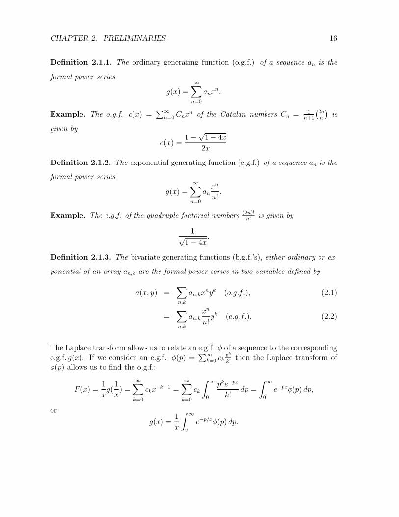
Definition 2.1.1. The ordinary generating function (o.g.f.) of a sequence an is the
formal power series
g(x) =
∞∑
n=0
anxn.
Example. The o.g.f. c(x) =∑∞
n=0Cnxn of the Catalan numbers Cn = 1
n+1
(
2nn
)
is
given by
c(x) =1 −
√1 − 4x
2x
Definition 2.1.2. The exponential generating function (e.g.f.) of a sequence an is the
formal power series
g(x) =
∞∑
n=0
anxn
n!.
Example. The e.g.f. of the quadruple factorial numbers (2n)!n!
is given by
1√1 − 4x
.
Definition 2.1.3. The bivariate generating functions (b.g.f.’s), either ordinary or ex-
ponential of an array an,k are the formal power series in two variables defined by
a(x, y) =∑
n,k
an,kxnyk (o.g.f.), (2.1)
=∑
n,k
an,kxn
n!yk (e.g.f.). (2.2)
The Laplace transform allows us to relate an e.g.f. φ of a sequence to the corresponding
o.g.f. g(x). If we consider an e.g.f. φ(p) =∑∞
k=0 ckpk
k!then the Laplace transform of
φ(p) allows us to find the o.g.f.:
F (x) =1
xg(
1
x) =
∞∑
k=0
ckx−k−1 =
∞∑
k=0
ck
∫ ∞
0
pke−px
k!dp =
∫ ∞
0
e−pxφ(p) dp,
or
g(x) =1
x
∫ ∞
0
e−p/xφ(p) dp.

CHAPTER 2. PRELIMINARIES 17
The coefficient of xn is denoted by [xn]g(x), and from the definition of the e.g.f., wehave n![xn]g(x) = [x
n
n!]g(x). For example [xn] 1√
1−4x=(
2nn
)
, the nth central binomial co-
efficient. Here, we use the operator [xn] to extract the nth coefficient of the power seriesg(x) [88]. We adopt the notation 0n = [xn]1 for the sequence 1, 0, 0, 0, . . . (A000007).The compositional inverse of a power series g =
∑
n=1 anxn with a1 6= 0 is a series
f =∑
n=1 bnxn with b1 6= 0 such that f ◦ g(x) = f(g(x)) =
∑
n≥1 bn(g(x))n = x. We
refer to the inverse of f as the series reversion f . We note that in some texts the seriesreversion is referred to by the notation f<−1>. Lagrange inversion [55] provides a simplemethod to calculate the coefficients of the series reversion.
Theorem 2.1.1. Lagrange Inversion Theorem [55, Theorem A.2]
Let φ(u) =∑∞
k=0 φkuk be a power series of C[[u]] with φ0 6= 0. Then, the equation
y = zφ(y) admits a unique solution in C[[u]] whose coefficients are given by
y(z) =
∞∑
n=1
ynzn, yn =
1
n[un−1]φ(u)n.
The Lagrange Inversion Theorem may be written as
[xn]G(f(x)) =1
n[xn−1]G′(x)
(
x
f(x)
)n
.
The simplest case is that of G(x) = x, in which we get
[xn]f(x) =1
n[xn−1]
(
x
f(x)
)n
.
Example. We have xc(x) = x(1 − x) and so we have
[xn]xc(x) =1
n[xn−1]
(
x
x(1 − x)
)n
=1
n[xn−1]
(
1
1 − x
)n
.
Thus,
[xn−1]c(x) =1
n[xn−1]
(
1
1 − x
)n
.
Changing n− 1 to n gives us
[xn]c(x) =1
n + 1[xn]
(
1
1 − x
)n+1
.
CHAPTER 2. PRELIMINARIES 18
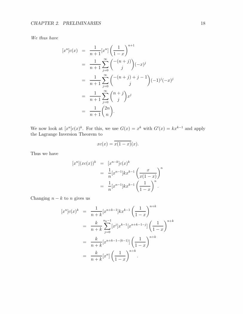
We thus have
[xn]c(x) =1
n + 1[xn]
(
1
1 − x
)n+1
=1
n + 1
∞∑
j=0
(−(n + j)
j
)
(−x)j
=1
n + 1
∞∑
j=0
(−(n + j) + j − 1
j
)
(−1)j(−x)j
=1
n + 1
∞∑
j=0
(
n + j
j
)
xj
=1
n + 1
(
2n
n
)
.
We now look at [xn]c(x)k. For this, we use G(x) = xk with G′(x) = kxk−1 and applythe Lagrange Inversion Theorem to
xc(x) = x(1 − x)(x).
Thus we have
[xn](xc(x))k = [xn−k]c(x)k
=1
n[xn−1]kxk−1
(
x
x(1 − x)
)n
=1
n[xn−1]kxk−1
(
1
1 − x
)n
.
Changing n− k to n gives us
[xn]c(x)k =1
n + k[xn+k−1]kxk−1
(
1
1 − x
)n+k
=k
n + k
nk−1∑
j=0
[xj ]xk−1[xn+k−1−j]
(
1
1 − x
)n+k
=k
n + k[xn+k−1−(k−1)]
(
1
1 − x
)n+k
=k
n + k[xn]
(
1
1 − x
)n+k
.

CHAPTER 2. PRELIMINARIES 19
Thus
[xn]c(x)k =k
n + k[xn]
(
1
1 − x
)n+k
.
We can simplify this using the Binomial Theorem. We get
[xn]c(x)k =k
n + k[xn]
(
1
1 − x
)n+k
=k
n + k[xn](1 − x)−(n+k)
=k
n + k[xn]
∞∑
j=0
(−(n + k)
j
)
(−x)j
=k
n + k[xn]
∞∑
j=0
(
n + k + j − 1
j
)
(−1)j(−x)j
=k
n + k[xn]
∞∑
j=0
(
n + k + j − 1
j
)
xj
=k
n + k
(
n + k + n− 1
n
)
=k
n + k
(
2n + k − 1
n
)
.
Thus we get
[xn]c(x)k =k
n + k[xn]
(
1
1 − x
)n+k
=k
n + k
(
2n + k − 1
n
)
.
Again, using Lagrange inversion, we have
[xn](xc(x))k =1
nk[xn−1]xk−1
(
1
1 − x
)n
.

CHAPTER 2. PRELIMINARIES 20
Thus
[xn](xc(x))k =k
n[xn−1]xk−1
(
1
1 − x
)n
=k
n[xn−1−k+1]
(
1
1 − x
)n
=k
n[xn−k]
(
1
1 − x
)n
=k
n[xn−k]
∞∑
j=0
(−n
j
)
(−x)j
=k
n
∞∑
j=0
(
n + j − 1
j
)
xj
=k
n
(
n + n− k − 1
n− k
)
=k
n
(
2n− k − 1
n− k
)
=k
n
n
2n− k
(
2n− k
n− k
)
=k
2n− k
(
2n− k
n− k
)
.
Adjusting this term for the case of n = 0, k = 0, we get [70]
[xn](xc(x))k =k + 0n+k
2n− k + 02n−k
(
2n− k
n− k
)
=k + 0n+k
2n− k + 02n−k
(
2n− k
n
)
.
By changing x to x2 in the above, we can easily arrive at expressions for [xn]c(x2)k
(this will give us the aerated versions of the sequences above). We prefer to use theLagrange Inversion Theorem again.
Our starting point is the observation that
xc(x2) =x
1 + x2.
Thus we we have
[xn](xc(x2))k = [xn−k]c(x2)k =1
n[xn−1]kxk−1
(
x1 + x2
x
)n
.

CHAPTER 2. PRELIMINARIES 21
Thus we have (changing n− k to n)
[xn]c(x2)k =k
n + k[xn+k−1]xk−1(1 + x2)n+k
=k
n + k
n+k−1∑
j=0
[xj ]xk−1[xn+k−1−j](1 + x2)n+k
=k
n + k[xn](1 + x2)n+k
=k
n + k[xn]
n+k∑
j=0
(
n + k
j
)
x2j
=k
n + k
(
n + kn2
)
1 + (−1)n
2.
Thus we have
[xn]c(x2)k =k
n + k[xn](1 + x2)n+k =
k
n + k
(
n + kn2
)
1 + (−1)n
2.
If the product of two power series f and g is 1 then f and g are termed reciprocalsequences and satisfy the following. For o.g.f.’s we have [161]
Definition 2.1.4. A reciprocal series g(x) =∑
n=0 anxn with a0 = 1, of a series
f(x) =∑
n=0 bnxn with b0 = 1, is a power series where g(x)f(x) = 1, which can be
calculated as follows
∞∑
n=0
anxn = −
∞∑
n=0
n∑
i=1
bian−ixn, a0 = 1 (2.3)
and for e.g.f.’s we have
Definition 2.1.5. A reciprocal series g(x) =∑
n=0 anxn
n!with a0 = 1, of a power series
f(x) =∑
n=0 bnxn
n!with b0 = 1, is a series where g(x)f(x) = 1, and can be calculated
as follows∞∑
n=0
anxn
n!= −
∞∑
n=0
n∑
i=1
(
n
k
)
bian−ixn
n!, a0 = 1. (2.4)

CHAPTER 2. PRELIMINARIES 22
2.2 The Riordan group
Riordan arrays give us an intuitive method of solving combinatorial problems, helpingto build an understanding of many number patterns. They provide an effective methodof proving combinatorial identities and solving numerical puzzles as in [86] rather thanusing computer based approaches [87, 141]. Riordan arrays, named after the combina-torist, John Riordan, 1 were first used in the 1990’s by Shapiro et al [119] as a methodof exploring combinatorial patterns in numbers of Pascal’s triangle. Shapiro saw thenatural extension of Pascal’s triangle due to its shape, to a lower triangular matrix,making use of matrix representation of transformations on sequences, then using thisto explore patterns in the numbers of Pascal’s triangle. This has become a classicalexample of a Riordan array. It was while exploring these extensions of Pascal’s tri-angle that it was realized that Riordan arrays have a group structure. Along withusing Riordan arrays as a method of proving combinatorial identities [134] they havealso been used in performing combinatorial sum inversions [133, 88]. In the past fewyears the idea of extending combinatorial theory to matrices as in Riordan arrays hasbeen extended to represent succession rules and the ECO method [135] which havebeen translated into the notion of Production matrices [36]. Articles such as [37] haveinvestigated the relationship between production matrices and Riordan arrays. Linksbetween generating trees and Riordan matrices have also been explored [85].
The Riordan group [118, 131, 115, 134, 121, 35] is a set of infinite lower-triangularinteger matrices, where each matrix is defined by a pair of generating functions g(x) =∑∞
n=0 gnxn with g0 = 1 and f(x) =
∑∞n=1 fnx
n with f1 6= 0 [131]. The associated ma-trix is the matrix whose i-th column is generated by g(x)f(x)i (the first column being
indexed by 0). This modifies to g(x)f(x)i
i!when we are concerned with exponential gen-
erating functions, leading to the exponential Riordan group. The matrix correspondingto the pair g, f is denoted by (g, f)(or [g, f ] in the exponential case). The group law isthen given by
(g, f) · (h, l) = (g(h ◦ f), l ◦ f).
The identity for this law is I = (1, x) and the inverse of (g, f) is (g, f)−1 = (1/(g◦ f), f)where f is the compositional inverse of f(f(x)) = f(f(x)).
If M is the matrix (g, f), and a = (a0, a1, . . .)′ is an integer sequence with o.g.f. A
1John Riordan spent much of his life working at Bell Laboratories(Bell Labs). His published
work includes “An Introduction to Combinatorics” published in 1978 and Combinatorial Identities,
published in 1968.

CHAPTER 2. PRELIMINARIES 23
(x), then the sequence Ma has o.g.f. g(x)A(f(x)). The (infinite) matrix (g, f) canthus be considered to act on the ring of integer sequences ZN by multiplication, wherea sequence is regarded as a (infinite) column vector. We can extend this action to thering of power series Z[[x]] by
(g, f) : A(x) 7→ (g, f) · A(x) = g(x)A(f(x)).
This result is called the fundamental theorem of Riordan arrays(FTRA).
Example. For ordinary generating functions, the so-called binomial matrix B is the
element ( 11−x
, x1−x
) of the Riordan group. It has general element(
nk
)
, and hence as an
array coincides with Pascal’s triangle. More generally, Bm is the element ( 11−mx
, x1−mx
)
of the Riordan group, with general term(
nk
)
mn−k. It is easy to show that the inverse
B−m of Bm is given by ( 11+mx
, x1+mx
).
Example. For exponential generating functions, the binomial matrix B is the element
[ex, x] of the Riordan group which as above, coincides with Pascal’s triangle. More
generally, Bm is the element [emx, x] of the Riordan group. It is easy to show that the
inverse B−m of Bm is given by [e−mx, x].
Multiplication of a matrix in the Riordan group by the binomial matrix (inverse Bi-nomial matrix) is what we will refer to as the Binomial transform (inverse Binomialtranform). In other words, BA will be called the binomial transform of A.
Example. If an has g.f. g(x), then the g.f. of the sequence
bn =
⌊n2⌋
∑
k=0
an−2k
is equal tog(x)
1 − x2=
(
1
1 − x2, x
)
· g(x).
The row sums of the matrix (g, f) have g.f.
(g, f) · 1
1 − x=
g(x)
1 − f(x),

CHAPTER 2. PRELIMINARIES 24
1
1 1
1 2 1
1 3 3 1
1 4 6 4 1
1 5 10 10 5 1
1 6 15 20 15 6 1
−→
1
1 1
1 2 1
1 3 3 1
1 4 6 4 1
1 5 10 10 5 1
1 6 15 20 15 6 1
Figure 2.1: Pascal’s triangle as a element of the Riordan group
while the diagonal sums of (g, f) (sums of left-to-right diagonals in the north east direc-tion) have g.f. g(x)/(1−xf(x)). These coincide with the row sums of the “generalized”Riordan array (g, xf). Thus the Fibonacci numbers Fn+1 are the diagonal sums of thebinomial matrix B given by
(
11−x
, x1−x
)
:
1 0 0 0 0 0 . . .1 1 0 0 0 0 . . .1 2 1 0 0 0 . . .1 3 3 1 0 0 . . .1 4 6 4 1 0 . . .1 5 10 10 5 1 . . ....
......
......
.... . .
while they are the row sums of the “generalized” or “stretched” (using the nomenclature
of [32] ) Riordan array(
11−x
, x2
1−x
)
:
1 0 0 0 0 0 . . .1 0 0 0 0 0 . . .1 1 0 0 0 0 . . .1 2 0 0 0 0 . . .1 3 1 0 0 0 . . .1 4 3 0 0 0 . . ....
......
......
.... . .
.

CHAPTER 2. PRELIMINARIES 25
We often work with “generalized” Riordan arrays, where we relax some of the con-ditions above. Thus for instance [32] discusses the notion of the “stretched” Riordanarray. In this note, we shall encounter “vertically stretched” arrays of the form (g, h)where now h0 = h1 = 0 with h2 6= 0. Such arrays are not invertible, but we may ex-plore their left inversion. In this context, standard Riordan arrays as described aboveare called “proper” Riordan arrays. We note for instance that for any proper Riordanarray (g, f), its diagonal sums are just the row sums of the vertically stretched array(g, xf) and hence have g.f. g/(1 − xf).
Each Riordan array (g(x), f(x)) has bivariate g.f. given by
g(x)
1 − yf(x).
For instance, the binomial matrix B has g.f.
11−x
1 − y x1−x
=1
1 − x(1 + y).
Similarly, exponential Riordan arrays [g(x), f(x)] have bivariate e.g.f. given by g(x)eyf(x).
For a sequence a0, a1, a2, . . . with g.f. g(x), the “aeration” of the sequence is thesequence a0, 0, a1, 0, a2, . . . with interpolated zeros. Its g.f. is g(x2). The sequencea0, a0, a1, a1, a2, . . . is called the “doubled” sequence. It has g.f. (1 + x)g(x2). Theaeration of a matrix M with general term mi,j is the matrix whose general term isgiven by
mri+j
2, i−j
2
1 + (−1)i−j
2,
where mri,j is the i, j-th element of the reversal of M:
mri,j = mi,i−j.
In the case of a Riordan array, the row sums of the aeration are equal to the diagonalsums of the reversal of the original matrix.
Example. The Riordan array (c(x2), xc(x2)) is the aeration of (c(x), xc(x)). Here
c(x) =1 −
√1 − 4x
2x

CHAPTER 2. PRELIMINARIES 26
is the g.f. of the Catalan numbers. The reversal of (c(x), xc(x)) is the matrix with
general element
[k ≤ n + 1]
(
n + k
k
)
n− k + 1
n + 1,
which begins
1 0 0 0 0 0 . . .
1 1 0 0 0 0 . . .
1 2 2 0 0 0 . . .
1 3 5 5 0 0 . . .
1 4 9 14 14 0 . . .
1 5 14 28 42 42 . . ....
......
......
.... . .
.
This is the Catalan triangle, A009766. Then (c(x2), xc(x2)) has general element
(
n + 1n−k2
)
k + 1
n + 1
(1 + (−1)n−k
2,
and begins
1 0 0 0 0 0 . . .
0 1 0 0 0 0 . . .
1 0 1 0 0 0 . . .
0 2 0 1 0 0 . . .
2 0 3 0 1 0 . . .
0 5 0 4 0 1 . . ....
......
......
.... . .
.
This is the “aerated” Catalan triangle, A053121. Note that
(c(x2), xc(x2)) =
(
1
1 + x2,
x
1 + x2
)−1
.

CHAPTER 2. PRELIMINARIES 27
We note that the diagonal sums of the reverse of (c(x), xc(x)) coincide with the row
sums of (c(x2), xc(x2)), and are equal to the central binomial coefficients(
n⌊n2⌋)
A001405.
2.3 Orthogonal polynomials
Orthogonal polynomials [27, 51, 63, 142, 144, 106] permeate many areas of mathematicswhich include algebra, combinatorics, numerical analysis, operator theory and randommatrices. The study of classic orthogonal polynomials dates back to the 18th century.By an orthogonal polynomial sequence (pn(x))n≥0 we shall understand an infinite se-quence of polynomials pn(x) where n ≥ 0, with real coefficients (often integer coeffi-cients) that are mutually orthogonal on an interval [x0, x1] (where x0 = −∞ is allowed,as well as x1 = ∞), with respect to a weight function w : [x0, x1] → R :
∫ x1
x0
pn(x)pm(x)w(x) dx = δnm√
hnhm,
where∫ x1
x0
p2n(x)w(x) dx = hn.
We assume that w is strictly positive on the interval (x0, x1). Referring to Favard’stheorem [27], every such sequence obeys a so-called “three-term recurrence” :
pn+1(x) = (anx + bn)pn(x) − cnpn−1(x)
for coefficients an, bn and cn that depend on n but not x. We note that if
pj(x) = kjxj + k′
jxj−1 + . . . j = 0, 1, . . .
then
an =kn+1
kn, bn = an
(
k′n+1
kn+1
− k′n
kn
)
, cn = an
(
kn−1hn
knhn−1
)
.
Since the degree of pn(x) is n, the coefficient array of the polynomials is a lower tri-angular (infinite) matrix. In the case of monic orthogonal polynomials the diagonalelements of this array will all be 1. In this case, we can write the three-term recurrenceas
pn+1(x) = (x− βn)pn(x) − αnpn−1(x), p0(x) = 1, p1(x) = x− β0.

CHAPTER 2. PRELIMINARIES 28
The moments associated to the orthogonal polynomial sequence are the numbers
µn =
∫ x1
x0
xnw(x) dx.
Theorem 2.3.1. [27, Theorem 3.1] A necessary and sufficient condition for the exis-
tence of an orthogonal polynomial sequence is
∆n = det(µi+j)ni,j≥0 =
∣
∣
∣
∣
∣
∣
∣
∣
∣
∣
∣
∣
µ0 µ1 . . . µn
µ1 µ2 . . . µn+1
...... . . .
...
µn µn+1 . . . µ2n
∣
∣
∣
∣
∣
∣
∣
∣
∣
∣
∣
∣
6= 0, n ≥ 0.
The matrix of moments above is a Hankel matrix, a matrix where the entry µn,k =µn+k. We will refer to the Hankel transform of a matrix which is the integer sequencegenerated by the successive Hankel determinants of a Hankel matrix. We can findpn(x), αn and βn from a knowledge of these moments. To do this, let ∆n,x be the samedeterminant as above, but with the last row replaced by 1, x, x2, . . . thus
∆n,x =
∣
∣
∣
∣
∣
∣
∣
∣
∣
µ0 µ1 . . . µn
µ1 µ2 . . . µn+1...
... . . ....
1 x . . . xn
∣
∣
∣
∣
∣
∣
∣
∣
∣
.
Then
pn(x) =∆n,x
∆n−1.
More generally, we let H
(
u1 . . . uk
v1 . . . vk
)
be the determinant of Hankel type with
(i, j)-th term µui+vj . That is
H
(
u1 . . . uk
v1 . . . vk
)
=
∣
∣
∣
∣
∣
∣
∣
∣
∣
µu1+v1 µu1+v2 . . . µu1+vk
µu2+v1 µu2+v2 . . . µu2+vk...
... . . ....
µuk+v1 µuk+v2 . . . µuk+vk
∣
∣
∣
∣
∣
∣
∣
∣
∣
Let
∆n = H
(
0 1 . . . n0 1 . . . n
)
, ∆′ = H
(
0 1 . . . n− 1 n0 1 . . . n− 1 n + 1
)
.

CHAPTER 2. PRELIMINARIES 29
Then we have
βn =∆′
n
∆n− ∆′
n−1
∆n−1, αn =
∆n−2∆n
∆2n−1
.
and the coefficient of xn−1 in pn(x) is −(β0 + β1 + β2 + · · · + βn).
Consider the three-term recurrence equation associated to the family of orthogonalpolynomials {pn(x)}n≥0:
pn+1(x) = (x− βn)pn(x) − αnpn−1(x).
Rearranging, this gives us
xpn(x) = αnpn−1(x) + βnpn(x) + pn+1(x),
expanding for the first few n we have
xp0(x) = α0p−1(x) + β0p0(x) + p1(x),
xp1(x) = α1p0(x) + β1p1(x) + p2(x),
xp2(x) = α2p1(x) + β2p2(x) + p3(x),
· · ·where p−1(x) = 0. Hence we get the following matrix equation
x
p0p1p2...
=
β0 1α1 β1 1
α2 β2 1. . .
p0p1p2...
.
Thus the matrix
J =
β0 1α1 β1 1
α2 β2 1. . .
represents multiplication by x on the space of polynomials, when we use the family{pn(x)}n≥0 as a basis.
We have
pn(x) =
∣
∣
∣
∣
∣
∣
∣
∣
∣
∣
∣
β0 − x 1α1 β1 − x 1
α2 β2 − x 1. . .
αn βn − x
∣
∣
∣
∣
∣
∣
∣
∣
∣
∣
∣
,

CHAPTER 2. PRELIMINARIES 30
that is, pn(x) is the characteristic polynomial of the n-th principal minor of J .
Example. The Chebyshev polynomials of the second kind, pn(x) = sin(n+1)θsin θ
, x =
cos θ, are orthogonal polynomials with respect to the weight√
1 − x2 on the interval
(-1,1). They obey the three term recurrence
pn+1(x) = 2xpn(x) − pn−1(x)
and the associated monic polynomials have the associated infinite tridiagonal matrix
J =
0 1 0 0 0 0 . . .
1 0 1 0 0 0 . . .
0 1 0 1 0 0 . . .
0 0 1 0 1 0 . . .
0 0 0 1 0 1 . . .
0 0 0 0 1 0 . . ....
......
......
.... . .
.
2.4 Continued fractions and the Stieltjes matrix
Two types of continued fraction which can be used to define formal power series are theJacobi (J-fraction) continued fraction and the Stieltjes (S-fraction) continued fraction.The J-fraction expansion for a power series f(x) =
∑∞n=0 anx
n has the form
1
1 − β0x− α1x2
1 − β1x− α2x2
1 − β2x− α3x2
. . .
, (2.5)

CHAPTER 2. PRELIMINARIES 31
and S-fraction expansion has the form
∞∑
n=0
anxn =
1
1 − α1x2
1 − α2x2
1 − α3x2
. . .
. (2.6)
At this point we note an important result due to Heilermann [76] which relates con-tinued fractions, as defined above, and orthogonal polynomials which we introduced insection 2.3.
Theorem 2.4.1. [76, Theorem 11] Let (an)n≥0 be a sequence of numbers with g.f.∑∞
n=0 anxn written in the form of
∞∑
n=0
anxn =
a0
1 − β0x−α1x
2
1 − β1x−α2x
2
. . .
.
Then the Hankel determinant hn of order n of the sequence (an)n≥0 is given by
hn = an0αn−11 αn−2
2 . . . α2n−1αn = an0
n∏
k=1
αn−kk
where the sequences {αn}n≥1 and {βn}n≥0 are the coefficients in the recurrence relation
Pn(x) = (x− βn)Pn−1(x) − αnPn−2(x), n = 1, 2, 3, 4, . . .
of the family of orthogonal polynomials Pn for which an forms the moment sequence.
The Hankel determinant [76] in the theorem above is a determinant of a matrix whichhas constant entries along antidiagonals. We previously encountered this matrix formin section 2.3, as the matrix of moments of orthogonal polynomials. The determinanthas the form
det0≤i,j≤n(ai+j).
CHAPTER 2. PRELIMINARIES 32
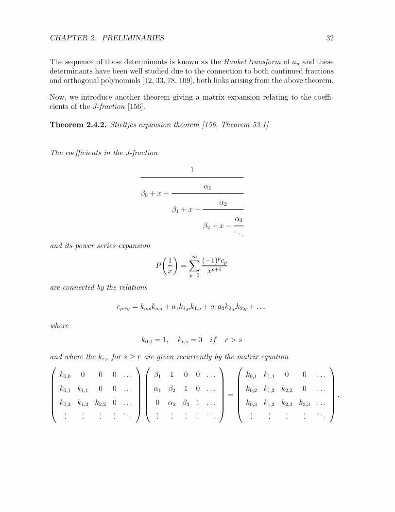
The sequence of these determinants is known as the Hankel transform of an and thesedeterminants have been well studied due to the connection to both continued fractionsand orthogonal polynomials [12, 33, 78, 109], both links arising from the above theorem.
Now, we introduce another theorem giving a matrix expansion relating to the coeffi-cients of the J-fraction [156].
Theorem 2.4.2. Stieltjes expansion theorem [156, Theorem 53.1]
The coefficients in the J-fraction
1
β0 + x−α1
β1 + x−α2
β2 + x−α3
. . .
and its power series expansion
P
(
1
x
)
=
∞∑
p=0
(−1)pcpxp+1
are connected by the relations
cp+q = ko,pko,q + a1k1,pk1,q + a1a2k2,pk2,q + . . .
where
k0,0 = 1, kr,s = 0 if r > s
and where the kr,s for s ≥ r are given recurrently by the matrix equation
k0,0 0 0 0 . . .
k0,1 k1,1 0 0 . . .
k0,2 k1,2 k2,2 0 . . ....
......
.... . .
β1 1 0 0 . . .
α1 β2 1 0 . . .
0 α2 β3 1 . . ....
......
.... . .
=
k0,1 k1,1 0 0 . . .
k0,2 k1,2 k2,2 0 . . .
k0,3 k1,3 k2,3 k3,3 . . ....
......
.... . .
.

CHAPTER 2. PRELIMINARIES 33
Relating this back to theorem 2.4.1, the link between continued fractions and orthog-onal polynomials can be seen once again, as we see the appearance of the tridiagonalmatrix relating to orthogonal polynomials, which we introduced in section 2.3. Notein the theorem above, we obtain the form of the J-fraction in Theorem (2.4.1) if wereplace the variable x by 1
xand divide by x.
In the context of Riordan arrays, we see the Stieltjes Expansion Theorem in [103],defined as follows
Definition 2.4.1. Let L = (lnk)n,k≥0 be a lower triangular matrix with li,i = 1 for all
i ≥ 0. The Stieltjes matrix SL associated with L is given by SL = L−1L where L is
obtained from L by deleting the first row of L, that is, the element in the nth row and
kth column of L is given by ln,k = ln+1,k
Using the definition of the Stieltjes matrix above [103] leads to the following theoremrelating the Riordan matrix to a Hankel matrix with a particular decomposition
Theorem 2.4.3. [103, Theorem 1] Let H = (hnk)n,k≥0 be the Hankel matrix generated
by the sequence 1, a1, a2, a3, . . . Assume that H = LDU where
L = (lnk)n,k≥0 =
1 0 0 0 . . .
l1,0 l1,0 0 0 . . .
l2,0 l2,1 1 0 . . .
l3,0 l3,1 l3,2 1 . . .
l4,0 l4,1 l4,2 l4,3 . . .
. . . . . . . . . . . . . . .
,
D =
d0 0 0 0 . . .
0 d1 0 0 . . .
0 0 d2 0 . . .
0 0 0 d3 . . ....
......
......
, di 6= 0, U = LT

CHAPTER 2. PRELIMINARIES 34
Then the Stieltjes matrix SL is tridiagonal, with the form
β0 1 0 0 0
α1 β1 1 0 . . .
0 α2 β2 1 . . .
0 0 α3 β3 . . .
0 0 0 α4 . . ....
......
.... . .
,
where
β0 = a1, α1 = d1, βk = lk+1,k − lk,k+1, αk+1 =dk+1
dk, k ≥ 0.
Now, we state two other relevant results from this paper, relating to generating func-tions which satisfy particular Stieltjes matrices. The first result relates to o.g.f.’s.
Theorem 2.4.4. [103, Theorem 2] Let H be the Hankel matrix generating by the
sequence 1, a1, a2, . . . and let H = LDLT. Then SL has the form
a1 1 0 0 . . .
α1 β 1 0 . . .
0 α β 1 . . .
0 0 α β . . .
0 0 0 α . . ....
......
.... . .
,
if and only if the o.g.f. g(x) of the sequence 1, a1, a2, . . . is given by
g(x) =1
1 − a1x− α1xf
where
f = x(1 + βf + αf 2).

CHAPTER 2. PRELIMINARIES 35
Peart and Woan [103] offer a proof of this in terms of the nth row of the Riordanmatrix. However the result can be deduced if we refer back to Theorem [76] relatingto J - fractions. Referring to Theorem [76] the Stieltjes matrix above has the relatedJ-fraction
g(x) =1
1 − a1x− α1x2
1 − βx− αx2
. . .
.
Now letting
f(x) =x
1 − βx− αx2
1 − βx− αx2
. . .
,
we have
g(x) =1
1 − a1x− α1xf(x).
Solving both equations above give us the required result. Similarly for e.g.f.’s we havethe following result
Theorem 2.4.5. [103, Theorem 3] Let H be the Hankel matrix generated by the se-
quence 1, a1, a2, . . . and let H = LDLT . Then SL has the form
β0 1 0 0 . . .
α1 β1 1 0 . . .
0 α2 β2 1 . . .
0 0 α3 β3 . . .
0 0 0 α4 . . ....
......
.... . .
,
if and only if the e.g.f. g(x) of the sequence 1, a1, a2, . . . is given by
g(x) =
∫
(a1 − α1f)dx, g(0) = 1

CHAPTER 2. PRELIMINARIES 36
wheredf
dx= 1 + βf + αf 2, f(0) = 0.
The proof again in [103] involves looking at the form of the nth column of the Riordanarray. However, intuitively this result can be seen from looking at the form of thematrix equation L = LS. In the case that L = [g(x), f(x)] is an exponential Riordanarray, we have the following
Proposition 2.4.6. L = ddx
(L) .
Proof.
d
dx
( ∞∑
n=0
gn(x)xn
n!
)
=
∞∑
n=1
gn(x)xn−1
(n− 1)!=
∞∑
n=0
gn+1(x)xn
(n)!
Equating the first columns of matrices L and LS we have
d
dx(g(x)) = β0g(x) + α1g(x)f(x)
and second columns equate to
d
dx(f(x)) = β1f(x) + α2f(x)2.
which gives us the required result.
The Stieltjes matrix as we have seen above is a tridiagonal infinite matrix which isassociated with orthogonal polynomials. However in the context of the Riordan group,we are concerned with general polynomials, and therefore have a generalization of theStieltjes matrix to the Riordan group. Referred to as a production matrix [36, 37], itis defined in the following terms.Let P be an infinite matrix (most often it will have integer entries). Letting r0 be therow vector
r0 = (1, 0, 0, 0, . . .),
we define ri = ri−1P where i ≥ 1. Stacking these rows leads to another infinite matrixwhich we denote by AP. Then P is said to be the production matrix for AP.

CHAPTER 2. PRELIMINARIES 37
If we letuT = (1, 0, 0, 0, . . . , 0, . . .)
then we have
AP =
uT
uTPuTP2
...
andDAP = APP
where D = (δi,j+1)i,j≥0. In [103, 115] P is called the Stieltjes matrix associated to AP.The sequence formed by the row sums of AP often has combinatorial significance andis called the sequence associated to P. Its general term an is given by an = uTPnewhere
e =
111...
In the context of ordinary Riordan arrays, the production matrix associated to a properRiordan array takes on a special form :
Proposition 2.4.7. [37] Let P be an infinite production matrix and let AP be the
matrix induced by P. Then AP is an (ordinary) Riordan matrix if and only if P is of
the form
P =
ξ0 α0 0 0 0 0 . . .
ξ1 α1 α0 0 0 0 . . .
ξ2 α2 α1 α0 0 0 . . .
ξ3 α3 α2 α1 α0 0 . . .
ξ4 α4 α3 α2 α1 α0 . . .
ξ5 α5 α4 α3 α2 α1 . . ....
......
......
.... . .
Moreover, columns 0 and 1 of the matrix P are the Z- and A-sequences, respectively,
of the Riordan array AP.

CHAPTER 2. PRELIMINARIES 38
We now introduce two results [36, 37, 35] concerning matrices that are productionmatrices for ordinary and exponential Riordan arrays which help us to recapture aknowledge of the Riordan array from the Stieltjes (production) matrices.
Proposition 2.4.8. Let P be a Riordan production matrix and let Z(x) and A(x) be
the generating functions of its first two columns, respectively. Then the bivariate g.f.
G(t, x) of the matrix AP induced by P and the g.f. fP (x) of the sequence induced by P
are given by
GP (t, x) =g(x)
1 − txf(x), fP (x) =
g(x)
1 − xf(x), (2.7)
where h(x) is determined from the equation
f(x) = A(xf(x)) (2.8)
and g(x) is given by
g(x) =1
1 − xZ(xf(x)). (2.9)
As a consequence
A(x) =x
f(x)
and
Z(x) =1
f(x)
(
1 − 1
g(f(x))
)
Proposition 2.4.9. [37, Proposition 4.1] [35] Let L = (ln,k)n,k≥0 = [g(x), f(x)] be an
exponential Riordan array and let
c(y) = c0 + c1y + c2y2 + . . . , r(y) = r0 + r1y + r2y
2 + . . . (2.10)
be two formal power series that that
r(f(x)) = f ′(x) (2.11)
c(f(x)) =g′(x)
g(x). (2.12)

CHAPTER 2. PRELIMINARIES 39
Then
(i) ln+1,0 =∑
i
i!ciln,i (2.13)
(ii) ln+1,k = r0ln,k−1 +1
k!
∑
i≥k
i!(ci−k + kri−k+1)ln,i (2.14)
or, assuming ck = 0 for k < 0 and rk = 0 for k < 0,
ln+1,k =1
k!
∑
i≥k−1
i!(ci−k + kri−k+1)ln,i. (2.15)
Conversely, starting from the sequences defined by (2.10), the infinite array (ln,k)n,k≥0
defined by (2.15) is an exponential Riordan array.
A consequence of this proposition is that the production matrix P = (pi,j)i,j≥0 for anexponential Riordan array obtained as in the proposition satisfies [37, 35]
pi,j =i!
j!(ci−j + jri−j+1) (c−1 = 0).
Furthermore, the bivariate e.g.f.
φP (t, x) =∑
n,k
pn,ktkx
n
n!
of the matrix P is given by
φP (t, x) = etx(c(x) + tr(x)),
where we haver(x) = f ′(f(x)), (2.16)
and
c(x) =g′(f(x))
g(f(x)). (2.17)

CHAPTER 2. PRELIMINARIES 40
2.5 Lattice paths
A lattice path [79] is a sequence of points in the integer lattice Z2. A pair of consecutivepoints is called a step of the path. A valuation is an integer function on the set ofpossible steps of Z2 × Z2. A valuation of a path is the product of the valuations of itssteps. We concern ourselves with two types of paths, Motzkin paths and Lukasiewiczpaths [151], which are defined as follows:
Definition 2.5.1. A Motzkin path [78] π = (π(0), π(1), . . . , π(n)), of length n, is a
lattice path starting at (0, 0) and ending at (n, 0) that satisfies the following conditions
1. The elementary steps can be north-east(N-E), east(E) and south-east(S-E).
2. Steps never go below the x axis.
Example. The four Motzkin paths for n = 3 are
x
y
x
y
x
y
x
y
Motzkin paths are counted by the Motzkin numbers, which have the g.f.
1 − x−√
1 − 2x− 3x2
2x2.
Dyck paths are Motzkin paths without the possibility of an East step.
Definition 2.5.2. A Lukasiewicz path [78] π = (π(0), π(1), . . . , π(n)), of length n, is a
lattice path starting at (0, 0) and ending at (n, 0) that satisfies the following conditions

CHAPTER 2. PRELIMINARIES 41
1. The elementary steps can be north-east(N-E) and east(E) as those in Motzkin
paths.
2. South-east(S-E) steps from level k can fall to any level above or on the x axis,
and are denoted as αn,k, where n is the length of the south-east step and k is the
level where the step ends.
3. Steps never go below the x axis.
Example. The five Lukasiewicz paths for n = 3 are
x
y
x
y
x
y
x
y
x
y
Theorem 2.5.1. [79, Theorem 2.3] Let
µn =∑
π∈Mv(π)
where the sum is over the set of Motzkin paths π = (π(0)....π(n)) of length n. Here
π(j) is the level after the jth step, and the valuation of a path is the product of the
valuations of its steps v(π) =∏n
i=1 vi where
vi = v(π(i− 1), π(i)) =
1 if the ith step rises
βπ(i−1) if the ith step is horizontal
απ(i−1) if the ith step falls

CHAPTER 2. PRELIMINARIES 42
1
level i βπ(i−1)
απ(i−1)
Then the g.f. of the sequence µn is given by
M(x) =∞∑
n=0
µnxn.
A continued fraction expansion of the g.f. is then
M(x) =1
1 − β0x−α1x
2
1 − β1x−α2x
2
1 − β2x−α3x
2
. . .
.
Example. A counting of a Motzkin path
x
β1
β2α3
α2
α1
y
v(π) = β1β2α1α2α3

CHAPTER 2. PRELIMINARIES 43
Similarly for Dyck paths we have
Theorem 2.5.2. Let
µn =∑
π∈Dv(π)
where the sum is over the set of Dyck paths π = (π(0)....π(n)) of length n. Here π(j) is
the level after the jth step, and the valuation of a path is the product of the valuations
of its steps v(π) =∏n
i=1 vi where
vi = v(π(i− 1), π(i)) =
1 if the ith step rises
απ(i−1) if the ith step falls
1
level i
απ(i−1)
Then the g.f. of the sequence µn is given by
D(x) =
∞∑
n=0
µnxn.
A continued fraction expansion of the g.f. is then
D(x) =1
1 −α1x
2
1 −α2x
2
1 −α3x
2
. . .
.
Example. A counting of a Dyck path

CHAPTER 2. PRELIMINARIES 44
x
α3
α2 α2
α1
y
v(π) = α1α22α3
M(x) corresponds to the J-fraction and D(x) corresponds to the S-fraction as in eq.(2.5) and eq. (2.6) respectively.
Letµn,k =
∑
π∈Mn,k
v(π)
where Mn,k is the set of Motzkin paths of length n from level 0 to level k, and v(π) isthe valuation of the path as in Theorem 2.5.1. Now, [56] defines vertical polynomialsVn(x) by
Vn(x) =n∑
i=0
µn,ixi
so we now introduce the following theorem:
Theorem 2.5.3. [151, Chapter 3, Proposition 7] Let {Pn(x)}n≥0 be a set of polyno-
mials satisfying the three term recurrence
Pn(x) = (x− βn)Pn−1(x) − αnPn−2(x) n = 1, 2, 3, 4, . . .
The vertical polynomials {Vn(x)}n≥0 are the inverse of the orthogonal polynomials
{Pn(x)}n≥0.
This means that the matrix P = (pn,k)0≤k≤n is the inverse of the matrix V = (µn,k)0≤k≤n.

CHAPTER 2. PRELIMINARIES 45
Example.
C(x) =1
1 − x−x2
1 − 2x−x2
1 − 2x−x2
. . .
.
The first few rows of P are
1 0 0 0 . . .
−1 1 0 0 . . .
1 −3 1 0 . . .
−1 6 −5 1 . . ....
......
.... . .
which is the Riordan array(
1
1 + x,
x
(1 + x)2
)
,
with inverse matrix (µn,k)0≤k≤n
1 0 0 0 . . .
1 1 0 0 . . .
2 3 1 0 . . .
5 9 5 1 . . ....
......
.... . .
,
which is the Riordan array(
c(x), c(x) − 1
)
.
To verify that µ3,1 = 9, we sum the weights of the following paths

CHAPTER 2. PRELIMINARIES 46
x
1·1· 1
y
x
1· 2· 2
y
x1· 1· 2
y
x1· 1· 1
y
x
1· 1· 1
y
Thus we have µ3,1 = 1 + 4 + 2 + 1 + 1 = 9.
We return to a theorem introduced previously [103], in which the Riordan array
L = (ln,k)n,k≥0
1 0 0 0 0 . . .l1,0 1 0 0 0 . . .l2,0 l2,1 1 0 0 . . .l3,0 l3,1 l3,2 1 0 . . .l4,0 l4,1 l4,2 l4,3 1 . . ....
......
......
. . .
was shown to satisfy the equations
ln,0 = β0ln−1,0 + α1ln−1,1,
andln,k = ln−1,k−1 + βkln−1,k + αkln−1,k+1. (2.18)
We now understand this equation in terms of Motzkin paths.
1. ln−1,k−1 −→ ln,k requires an added north-east(N-E) step at the end of each pathwith the path value unchanged as the N-E step is 1.
2. ln−1,k+1 −→ ln,k requires an added south-east(S-E) step at the end of each path,changing the path value by αk, the value defined in Theorem 2.5.1 for each S-Estep.

CHAPTER 2. PRELIMINARIES 47
3. ln−1,k −→ ln,k requires an added east(E) step at the end of each path, changingthe path value by βk, the value defined in Theorem 2.5.1 for each E step.
Example. Here we use the Riordan array, ( c(x)−1x
, xc(x) − 1) to illustrate.
L =
1 0 0 0 0 . . .
2 1 0 0 0 . . .
5 4 1 0 0 . . .
14 14 6 1 1 . . .
42 48 27 8 1 . . ....
......
......
. . .
.
We calculate l4,1 using eq. (2.18) above, thus
l4,1 = l3,0 + 2l3,1 + l3,2.
We note that the level steps have weight two which can be seen from the continued
fraction expansion of the g.f. of the Catalan numbers which has the form
c(x) − 1
x=
1
1 − 2x−x2
1 − 2x−x2
1 − 2x−x2
. . .
.
We now count each of the Motzkin paths l3,0, l3,1, l3,2, and adjust each path according to
the steps laid out above. Each adjustment to the lattice path is highlighted in red.
Firstly, the paths below are those of length three and final level zero, l3,0, and an added
N-E step of weight one.

CHAPTER 2. PRELIMINARIES 48
x
1 ·1 ·2 ·1
y
x
1·2 ·1 ·1
y
x2· 1· 1· 1
y
x2 · 2 · 2
·1
y
We now look at the paths of length three and final level one l3,1, and an added E step
of weight two.
x2
·1 ·2 ·2y
x2 · 2· 1· 2
y
x
1· 2 · 2 ·2y
x
1 · 1· 1·2
y
x
1· 1· 1·2
y
Finally, the paths below are those of length three and final level two, l3,2, and an added
S-E step of weight one.
x
1· 2· 1· 1y
x
1·1· 2 ·1
y
x2·
1 · 1·1
y
Summing over all paths above gives
l4,1 = l3,0 + 2l3,1 + l3,2 = 14 + 2(14) + 6 = 48.

Chapter 3
Chebyshev Polynomials
In this chapter we introduce the Chebyshev polynomials named after the 19th centuryRussian mathematician Pafnuty Chebyshev, which have been studied in detail becauseof their relevance in many fields of mathematics. One use of Chebyshev polynomialsis in the field of wireless communication where Chebyshev filters are based on theChebyshev polynomials. We note that Chebyshev polynomials have also been used inthe calculation of MIMO systems [71]. MIMO systems are of interest to us in Chapter8. This chapter is broken down into two sections. In the first section we introduce theChebyshev polynomials and the properties of interest to us and show the formation ofthe related Riordan arrays through their matrices of coefficients. We summarize theseresults in the table in Fig. 3.1. Inspired by Estelle Basor and Torsten Ehrhardt [18]we extend results relating determinants of Hankel plus Toeplitz matrices and Hankelmatrices relating to the Chebyshev polynomials of the third kind, to the Chebyshevpolynomials of the first and second kind using properties of the polynomials we havedrawn to the readers attention in the first section. Note that we look at the polynomialsin reverse order as the polynomials of the third kind are those from [18], so are a naturalstarting point for our study.
49

CHAPTER 3. CHEBYSHEV POLYNOMIALS 50
3.1 Introduction to Chebyshev polynomials
We begin this section by recalling some facts about the Chebyshev polynomials of thefirst, second and third kind [112].
The Chebyshev polynomials of the second kind, Un(x), can be defined by
Un(x) =
⌊n2⌋
∑
k=0
(
n− k
k
)
(−1)k(2x)n−2k, (3.1)
or alternatively as
Un(x) =
n∑
k=0
(
n+k2
k
)
(−1)n−k2
1 + (−1)n−k
2(2x)k. (3.2)
The g.f. is given by∞∑
n=0
Un(x)tn =1
1 − 2xt + t2.
The Chebyshev polynomials of the second kind, Un(x), which begin
1, 2x, 4x2 − 1, 8x3 − 4x, 16x4 − 12x2 + 1, 32x5 − 32x3 + 6x, . . .
have coefficient array
1 0 0 0 0 0 . . .0 2 0 0 0 0 . . .−1 0 4 0 0 0 . . .0 −4 0 8 0 0 . . .1 0 −12 0 16 0 . . .0 6 0 −32 0 32 . . ....
......
......
.... . .
. (A053117)
This is the (generalized) Riordan array(
1
1 + x2,
2x
1 + x2
)
.
We note that the coefficient array of the modified Chebyshev polynomials Un(x/2)which begin
1, x, x2 − 1, x3 − 2x, x4 − 3x2 + 1, . . . ,

CHAPTER 3. CHEBYSHEV POLYNOMIALS 51
is given by
1 0 0 0 0 0 . . .0 1 0 0 0 0 . . .−1 0 1 0 0 0 . . .0 −2 0 1 0 0 . . .1 0 −3 0 1 0 . . .0 3 0 −4 0 1 . . ....
......
......
.... . .
. (A049310)
This is the Riordan array(
1
1 + x2,
x
1 + x2
)
,
with inverse
1 0 0 0 0 0 . . .0 1 0 0 0 0 . . .1 0 1 0 0 0 . . .0 2 0 1 0 0 . . .2 0 3 0 1 0 . . .0 5 0 4 0 1 . . .5 0 9 0 5 0 . . ....
......
......
.... . .
, (A053121)
which is the Riordan array(
c(x2), xc(x2))
.
c(x) =1 −
√1 − 4x
2x
is the g.f. of the Catalan numbers Cn = 1n+1
(
2nn
)
. The Chebyshev polynomials of thesecond kind satisfy the recurrence relation,
Un(x) = 2xUn−1(x) − Un−2(x)
and by the change of variable from x to x/2 we have
Un(x/2) = xUn−1(x/2) − Un−2(x/2),

CHAPTER 3. CHEBYSHEV POLYNOMIALS 52
for the modified polynomials, with corresponding Stieltjes matrix
0 1 0 0 0 0 . . .1 0 1 0 0 0 . . .0 1 0 1 0 0 . . .0 0 1 0 1 0 . . .0 0 0 1 0 1 . . .0 0 0 0 1 0 . . .0 0 0 0 0 1 . . ....
......
......
.... . .
.
The Chebyshev polynomials of the third kind can be defined as
Vn(x) =
⌊n−12
⌋∑
k=0
(−1)k(
n− 1 − kk
)
(2x)n−1−2k(
(−1)⌊n2⌋ − 1
)
with g.f.∞∑
k=0
Vn(x)tn =1 − t
1 − 2xt + t2.
They relate to the Chebyshev polynomials of the second kind by the equation
Vn(x) = Un(x) − Un−1(x).
The Chebyshev polynomials of the third kind, Vn(x) which begin
1, 2x− 1, 4x2 − 2x− 1, 8x3 − 4x2 − 4x + 1 . . .
have coefficient array
1 0 0 0 0 0 . . .−1 2 0 0 0 0 . . .−1 −2 4 0 0 0 . . .1 −4 −4 8 0 0 . . .1 −4 −4 −8 16 0 . . ....
......
......
.... . .
.
This is the (generalized) Riordan array(
1 − x
1 + x2,
2x
1 + x2
)
.

CHAPTER 3. CHEBYSHEV POLYNOMIALS 53
We note that the coefficient array of the modified Chebyshev polynomials Vn(x/2)which begin
1, x− 1, x2 − x− 1, x3 − x2 − 2x + 1 . . .
is given by
1 0 0 0 0 0 . . .−1 1 0 0 0 0 . . .−1 −1 1 0 0 0 . . .1 −2 −1 1 0 0 . . .1 2 −3 −1 1 0 . . ....
......
......
.... . .
.
This is the Riordan array(
1 − x
1 + x2,
x
1 + x2
)
,
with inverse,
1 0 0 0 0 0 . . .1 1 0 0 0 0 . . .2 1 1 0 0 0 . . .3 3 1 1 0 0 . . .6 4 4 1 1 0 . . .10 10 5 5 1 1 . . ....
......
......
.... . .
, (A061554)
which is the Riordan array(1 + xc(x2)√
1 − 4x2, xc(x2)
)
.
The Chebyshev polynomials of the third kind Vn satisfy the recurrence relation,
Vn+1(x) = 2xVn(x) − Vn−1(x),
with corresponding Stieltjes matrix for Vn(x/2), given by
1 1 0 0 0 0 01 0 1 0 0 0 00 1 0 1 0 0 00 0 1 0 1 0 00 0 0 1 0 1 00 0 0 0 1 0 10 0 0 0 0 1 0...
......
......
.... . .
.

CHAPTER 3. CHEBYSHEV POLYNOMIALS 54
Again we note that the Chebyshev polynomials of the fourth kind, Wn(x) are simply thethird polynomials with a change of sign. Related Riordan arrays for these polynomialscan be seen in the table below.
The Chebyshev polynomials of the first kind, Tn(x), are defined by
Tn(x) =n
2
⌊n2⌋
∑
k=0
(
n− k
k
)
(−1)k
n− k(2x)n−2k (3.3)
for n > 0, and T0(x) = 1. The first few Chebyshev polynomials of the first kind are
1, x, 2x2 − 1, 4x3 − 3x . . .
and have g.f.∞∑
n=0
Tn(x)tn =1 − xt
1 − 2xt + t2,
They satisfy the recurrence relation
Tn+1(x) = 2xTn(x) − Tn−1(x).
The situation with the Chebyshev polynomials of the first kind differs slightly, sincewhile the coefficient array of the polynomials 2Tn(x) − 0n, which begins
1 0 0 0 0 0 . . .0 2 0 0 0 0 . . .−2 0 4 0 0 0 . . .0 −6 0 8 0 0 . . .2 0 −16 0 16 0 . . .0 10 0 −40 0 32 . . ....
......
......
.... . .
,
is a (generalized) Riordan array, namely
(
1 − x2
1 + x2,
2x
1 + x2
)
,

CHAPTER 3. CHEBYSHEV POLYNOMIALS 55
that of Tn(x), which begins
1 0 0 0 0 0 . . .0 1 0 0 0 0 . . .−1 0 2 0 0 0 . . .0 −3 0 4 0 0 . . .1 0 −8 0 8 0 . . .0 5 0 −20 0 16 . . ....
......
......
.... . .
(A053120)
is not a generalized Riordan array. However the Riordan array
(
1 − x2
1 + x2,
x
1 + x2
)
which begins
1 0 0 0 0 0 . . .0 1 0 0 0 0 . . .−2 0 1 0 0 0 . . .0 −3 0 1 0 0 . . .2 0 −4 0 1 0 . . .0 5 0 −5 0 1 . . ....
......
......
.... . .
(A108045)
is the coefficient array for the orthogonal polynomials given by (2 − 0n)Tn(x/2).
We see from the table in Fig. 3.1 that the inverse of the matrix of coefficients of the
Chebyshev polynomials has Riordan array of the form(
g(x), xc(x2))
, with kth column
generated by g(x)(xc(x2))k. For this reason we introduce and prove the next identitybefore continuing to the next section.
Proposition 3.1.1.
(xc(x2))m = c(x2)
⌊m−12
⌋∑
k=0
(−1)k(
m− k − 1
k
)
x2k−m+2 −⌊m−2
2⌋
∑
k=0
(−1)k(
m− k − 2
k
)
x2k−m+2
(3.4)

CHAPTER 3. CHEBYSHEV POLYNOMIALS 56
Chebyshev polynomial Stieltjes matrix Coefficient Inverse coefficient
array array
Tn(x) = 1, x, 2x2 − 1, 4x3 − 3x, . . .
0 2 0 . . .
1 0 1 . . .
0 1 0 . . ....
......
. . .
(
1−x2
1+x2 ,2x
1+x2
)
(2− 0)Tn(x/2) = 1, x, x2 − 2x3 . . .
0 1 0 . . .
2 0 1 . . .
0 1 0 . . ....
......
. . .
(
1−x2
1+x2 ,x
1+x2
) (
1√1−4x2
, xc(x2)
)
Un(x) = 1, 2x, 4x2 − 1, 8x3 − 4x . . .
0 1 0 . . .
1 0 1 . . .
0 1 0 . . ....
......
. . .
(
11+x2 ,
x1+x2
)
(
c(x2), xc(x2))
Vn(x) = 1, 2x− 1, 4x2 − 2x− 1 . . .
1 1 0 . . .
1 0 1 . . .
0 1 0 . . ....
......
. . .
(
1−x1+x2 ,
x1+x2
) (
1+xc(x2)√1−4x2
, xc(x2)
)
Wn(x) = 1, 2x + 1, 4x2 + 2x− 1 . . .
−1 1 0 . . .
1 0 1 . . .
0 1 0 . . ....
......
. . .
(
1+x1+x2 ,
x1+x2
)
( √1−4x2−1√
1−4x2−2x−1, xc(x2)
)
Figure 3.1: Chebyshev polynomials and related Riordan arrays

CHAPTER 3. CHEBYSHEV POLYNOMIALS 57
Proof. Firstly, it is clear that the identity holds true for m = 1. We now assume true
for m, and endeavor to prove by induction that
(xc(x2))m+1 = c(x2)
⌊m2⌋
∑
k=0
(−1)k(
m− k
k
)
x2k−m+1 −⌊m−1
2⌋
∑
k=0
(−1)k(
m− k − 1
k
)
x2k−m+1
(3.5)
Expanding (xc(x2))(xc(x2))m we have
(xc(x2))2⌊m−1
2⌋
∑
k=0
(−1)k(
m− k − 1
k
)
x2k−m+2 − xc(x2)
⌊m−22
⌋∑
k=0
(−1)k(
m− k − 2
k
)
x2k−m+2
which expands further as
c(x2)
( ⌊m−12
⌋∑
k=0
(−1)k(
m− k − 1
k
)
x2k−m+1 −⌊m−2
2⌋
∑
k=0
(−1)k(
m− k − 2
k
)
x2k−m+3
)
−⌊m−1
2⌋
∑
k=0
(−1)k(
m− k − 1
k
)
x2k−m+1.
Now, to sum over possible values of x, we change the summation of
⌊m−22
⌋∑
k=0
(−1)k(
m− k − 2
k
)
x2k−m+3,
to become
⌊m2⌋−1∑
k=1
(−1)(k−1)
(
m− k − 1
k − 1
)
x2k−m+1 − (−1)⌊m2⌋(
m− ⌊m2⌋ − 1
⌊m2⌋ − 1
)
x2⌊m2⌋−m+1.
Now with the above changed summation (xc(x2))m+1 becomes
c(x2)
( ⌊m−12
⌋∑
k=0
(−1)k(
m− k − 1
k
)
x2k−m+1 +
⌊m2⌋−1∑
k=1
(−1)k(
m− k − 1
k − 1
)
x2k−m+1+
(−1)⌊m2⌋(
m− ⌊m2⌋ − 1
⌊m2⌋ − 1
)
x2⌊m2⌋−m+1
)
−⌊m−1
2⌋
∑
k=0
(−1)k(
m− k − 1
k
)
x2k−m+1.

CHAPTER 3. CHEBYSHEV POLYNOMIALS 58
Next, we will simplify further investigating separately the terms for m even and odd.
For m odd, (xc(x2))m+1 becomes
c(x2)
(
x−m+1+
⌊m2⌋−1∑
k=1
(−1)k(
m− k
k
)
x2k−m+1+(−1)⌊m−1
2⌋(
m− (⌊m−12
⌋) − 1
⌊m−12
⌋
)
x2(⌊m−12
⌋)−m+1
+(−1)⌊m2⌋(
m− ⌊m2⌋ − 1
⌊m2⌋ − 1
)
x2⌊m2⌋−m+1
)
−⌊m−1
2⌋
∑
k=0
(−1)k(
m− k − 1
k
)
x2k−m+1
which simplifies to
c(x2)
( ⌊m2⌋−1∑
k=0
(−1)k(
m− k
k
)
x2k−m+1 + (−1)m−1
2
((m−12
m−12
)
+
( m−12
m−12
− 1
))
x2m−12
−m+1
)
−⌊m−1
2⌋
∑
k=0
(−1)k(
m− k − 1
k
)
x2k−m+1
thus
(xc(x2))m+1 = c(x2)
( ⌊m2⌋−1∑
k=0
(−1)k(
m− k
k
)
x2k−m+1 + (−1)m−1
2
((m+12
m−12
))
x2m−12
−m+1
)
−⌊m−1
2⌋
∑
k=0
(−1)k(
m− k − 1
k
)
x2k−m+1
= c(x2)
( ⌊m2⌋
∑
k=0
(−1)k(
m− k
k
)
x2k−m+1
)
−⌊m−1
2⌋
∑
k=0
(−1)k(
m− k − 1
k
)
x2k−m+1.
This gives eq. (3.4). Similarly, for m even, we have (xc(x2))m+1 as
c(x2)
( ⌊m2⌋−1∑
k=0
(−1)k(
m− k
k
)
x2k−m+1+(−1)⌊m2⌋x2⌊m
2⌋−m+1
)
−⌊m−1
2⌋
∑
k=0
(−1)k(
m− k − 1
k
)
x2k−m+1
thus
(xc(x2))m+1 = c(x2)
⌊m2⌋
∑
k=0
(−1)k(
m− k
k
)
x2k−m+1 −⌊m−1
2⌋
∑
k=0
(−1)k(
m− k − 1
k
)
x2k−m+1
which also gives eq. (3.4), and completes the induction.

CHAPTER 3. CHEBYSHEV POLYNOMIALS 59
Corollary 3.1.2. For m even
∞∑
r=1
⌊m−12
⌋∑
k=0
(−1)k1
2(2r − 1 + m− 2k)
(
m− k − 1
k
)(
2r + m− 2k2r+m−2k
2
)
x2r (3.6)
and for m odd,
∞∑
r=1
⌊m−12
⌋∑
k=0
(−1)k1
2(−2k + m + 2r)
(
m− k − 1
k
)(
2r + m + 1 − 2k2r+m+1−2k
2
)
x2r+1 (3.7)
Now, we simplify eq. 3.4,
c(x2)
⌊m−12
⌋∑
k=0
(−1)k(
m− k − 1
k
)
x2k−m+2 −⌊m−2
2⌋
∑
k=0
(−1)k(
m− k − 2
k
)
x2k−m+2
= −∞∑
n=0
1
1 − 2n
(
2n
n
)
x2n
2
⌊m−12
⌋∑
k=0
(−1)k(
m− k − 1
k
)
x2k−m +1
2
⌊m−12
⌋∑
k=0
(−1)k(
m− k − 1
k
)
x2k−m
−⌊m−2
2⌋
∑
k=0
(−1)k(
m− k − 2
k
)
x2k−m+2
= −(
1
2
⌊m−12
⌋∑
k=0
(−1)k(
m− k − 1
k
)
x2k−m +∞∑
n=1
1
1 − 2n
(
2n
n
)
x2n
2
) ⌊m−12
⌋∑
k=0
(−1)k(
m− k − 1
k
)
x2k−m
+1
2
⌊m−12
⌋∑
k=0
(−1)k(
m− k − 1
k
)
x2k−m −⌊m−2
2⌋
∑
k=0
(−1)k(
m− k − 2
k
)
x2k−m+2
=∞∑
n=0
1
2(1 + 2n)
(
2n + 2
n + 1
)
x2n+2
⌊m−12
⌋∑
k=0
(−1)k(
m− k − 1
k
)
x2k−m
−⌊m−2
2⌋
∑
k=0
(−1)k(
m− k − 2
k
)
x2k−m+2
now we have
1
2xm
⌊m−12
⌋∑
n=0
n∑
k=0
(−1)k1
1 + 2n− 2k
(
m− k − 1
k
)(
2n + 2 − 2k
n + 1 − k
)
x2n+2

CHAPTER 3. CHEBYSHEV POLYNOMIALS 60
+1
2xm
∞∑
n=⌊m+12
⌋
⌊m−12
⌋∑
k=0
(−1)k1
1 + 2n− 2k
(
m− k − 1
k
)(
2n + 2 − 2k
n + 1 − k
)
x2n+2
−⌊m−2
2⌋
∑
k=0
(−1)k(
m− k − 2
k
)
x2k−m+2
For m > 1
1
2xm
⌊m−12
⌋∑
n=0
n∑
k=0
(−1)k1
1 + 2n− 2k
(
m− k − 1
k
)(
2n + 2 − 2k
n + 1 − k
)
x2n+2
=
⌊m−22
⌋∑
k=0
(−1)k(
m− k − 2
k
)
x2k−m+2
Now for m > 1, we have
(xc(x2))m =1
2
∞∑
n=⌊m+12
⌋
⌊m−12
⌋∑
k=0
(−1)k1
1 + 2n− 2k
(
m− k − 1
k
)(
2n + 2 − 2k
n + 1 − k
)
x2n+2−m
(3.8)Extracting odd and even terms gives the required result.
3.2 Toeplitz-plus-Hankel matrices and the family of
Chebyshev polynomials
We extend results from [18], relating determinants of Hankel matrices to determinantsof Toeplitz-plus-Hankel matrices, to the family of Chebyshev polynomials using Rior-dan arrays. Firstly, we take this opportunity to present the relevant result from [18].We observe the relationship between the Toeplitz-plus-Hankel matrices, Hankel matri-ces and the matrix of the inverse of the coefficients of the Chebyshev polynomials ofthe third kind. We provide an alternative proof of this result through the medium ofRiordan arrays. We then extend these results to Toeplitz-plus-Hankel matrices relatingto the first and second Chebyshev polynomials.

CHAPTER 3. CHEBYSHEV POLYNOMIALS 61
3.2.1 Chebyshev polynomials of the third kind
Theorem 3.2.1. [18, Proposition 2.1] Let {an}∞n=−∞ be a sequence of complex numbers
such that an = a−n and let {bn}∞n=1 be a sequence defined by
bn =n−1∑
k=0
(
n− 1
k
)
(a1−n+2k + a2−n+2k). (3.9)
Define the one-sided infinite matrices
A = (aj−k + aj+k+1)∞j,k=0 B = (bj+k+1)
∞j,k=0
and the upper triangular one-sided infinite matrix
D =
ξ(0, 0) ξ(1, 1) ξ(2, 2) . . .
ξ(1, 0) ξ(2, 1) . . .
ξ(2, 0) . . .. . .
where ξ(n, k) =(
n⌊n−k
2⌋)
. Then B = DTAD.
We note that DT = L is the Riordan array
L =
(
1 + xc(x2)√1 − 4x2
, xc(x2)
)
and(1 + xc(x2)√
1 − 4x2, xc(x2)
)−1
=( 1 − x
1 + x2,
x
1 + x2
)
.
Referring back to the table in Fig. (3.1) we see that the Riordan array above is theRiordan array of the inverse of the coefficients of the Chebyshev polynomials of thethird kind.
This result is the preliminary result in [18] showing the relationship between certainsymmetric Toeplitz-plus-Hankel matrices and Hankel matrices. This preliminary resultleads to the following result connecting determinants of these matrices.

CHAPTER 3. CHEBYSHEV POLYNOMIALS 62
Theorem 3.2.2. [18, Theorem 2.2] Let {an}∞n=−∞ and {bn}∞n=1 fulfill the assumptions
of the previous proposition. For N ≥ 1 define the matrices
AN = (aj−k + aj+k+1)N−1j,k=0, BN = (bj+k+1)
N−1j,k=0
Then detAN = detBN .
With the aid of Riordan arrays, we define a transformation B. We then show that thistransformation is equivalent to the transformation bn =
∑
k=0
(
nk
)
(a|n−2k| + a|n−2k+1|).
The g.f. of the central binomial coefficients(
n⌊n2⌋)
is given by
1 + (xc(x2))2
1 − xc(x2)=
√1 − 4x2 + 2x− 1
2x(1 − 2x).
We can show that the coefficient array of the orthogonal polynomials with weight√4−x2
2−x
is the matrix(
1 − x
1 + x2,
x
1 + x2
)
.
We have(
1 − x
1 + x2,
x
1 + x2
)−1
=
(
1 + (xc(x2))2
1 − xc(x2), xc(x2)
)
:= L,
with general term(
nn−k2
)
.
Then the LDU decomposition of the Hankel matrix H = H( n
⌊n2 ⌋)
for(
n⌊n2⌋)
is given by
H = L · I · Lt = LLt,
where the diagonal matrix is the identity since the Hankel transform of(
n⌊n2⌋)
is all 1’s.
Now we have the following identity of Riordan arrays
(
1
1 + x, x
)
·(
1 − x2
1 + x2,
x
1 + x2
)
=
(
1 − x
1 + x2,
x
1 + x2
)
.

CHAPTER 3. CHEBYSHEV POLYNOMIALS 63
Thus
L =
(
1 − x
1 + x2,
x
1 + x2
)−1
=
(
1 − x2
1 + x2,
x
1 + x2
)−1
·(
1
1 + x, x
)−1
=
(
1 − x2
1 + x2,
x
1 + x2
)−1
· (1 + x, x) ,
where(
1 − x2
1 + x2,
x
1 + x2
)−1
is the matrix with general term
(
nn−k2
)
1 + (−1)n−k
2.
Thus we have
H =
(
1 − x2
1 + x2,
x
1 + x2
)−1
· (1 + x, x) · (1 + x, x)t(
(
1 − x2
1 + x2,
x
1 + x2
)−1)t
,
where(1 + x, x) · (1 + x, x)t
is the matrix
1 1 0 0 0 0 . . .1 2 1 0 0 0 . . .0 1 2 1 0 0 . . .0 0 1 2 1 0 . . .0 0 0 1 2 1 . . .0 0 0 0 1 2 . . ....
......
......
.... . .
.
We now form the matrix
B = L · (1 + x, x)t =
(
1 − x2
1 + x2,
x
1 + x2
)−1
· (1 + x, x) · (1 + x, x)t .

CHAPTER 3. CHEBYSHEV POLYNOMIALS 64
This matrix begins
B =
1 1 0 0 0 0 . . .1 2 1 0 0 0 . . .2 3 2 1 0 0 . . .3 6 4 2 1 0 . . .6 10 8 5 2 1 . . .10 20 15 10 6 2 . . ....
......
......
.... . .
.
We note that the matrix B is the matrix formed from expanding eq. (3.9), that is
b1b2b3b4b5...
=
1 1 0 0 0 0 . . .1 2 1 0 0 0 . . .2 3 2 1 0 0 . . .3 6 4 2 1 0 . . .6 10 8 5 2 1 . . .10 20 15 10 6 2 . . ....
......
......
.... . .
a0a1a2a3a4...
.
We can regard this as the Riordan array
(
1 − x
(1 + x)(1 + x2),
x
1 + x2
)−1
=
(
(1 + 2x)c(x2)√1 − 4x2
, xc(x2)
)
,
with a column with elements(
n⌊n2⌋)
prepended. Alternatively, we can regard it as a
“beheaded” version of the Riordan array
(
1 − x
1 + x,
x
1 + x2
)−1
=
(
1 + 2x√1 − 4x2
, xc(x2)
)
,
where the first column terms are divided by 2.
By definition, we have
H( n⌊n2 ⌋)
= B ·(
(
1 − x2
1 + x2,
x
1 + x2
)−1)t
= B · (c(x2), xc(x2))t.

CHAPTER 3. CHEBYSHEV POLYNOMIALS 65
We can derive an expression for the general term of B in the following manner. De-compose (1 + x, x) · (1 + x, x)t as the sum of two matrices:
1 0 0 0 0 0 . . .1 1 0 0 0 0 . . .0 1 1 0 0 0 . . .0 0 1 1 0 0 . . .0 0 0 1 1 0 . . .0 0 0 0 1 1 . . ....
......
......
.... . .
+
0 1 0 0 0 0 . . .0 1 1 0 0 0 . . .0 0 1 1 0 0 . . .0 0 0 1 1 0 . . .0 0 0 0 1 1 . . .0 0 0 0 0 1 . . ....
......
......
.... . .
,
which is (1 + x, x) and a shifted version of (1 + x, x). To obtain B we multiply by(
1−x2
1+x2 ,x
1+x2
)
. This gives us
B =
1 0 0 0 0 0 . . .1 1 0 0 0 0 . . .2 1 1 0 0 0 . . .3 3 1 1 0 0 . . .6 4 4 1 1 0 . . .10 10 5 5 1 1 . . ....
......
......
.... . .
+
0 1 0 0 0 0 . . .0 1 1 0 0 0 . . .0 2 1 1 0 0 . . .0 3 3 1 1 0 . . .0 6 4 4 1 1 . . .0 10 10 5 5 1 . . ....
......
......
.... . .
,
where the first member of the sum is the Riordan array(
1 − x2
1 + x2,
x
1 + x2
)−1
· (1 + x, x) =
(
1 − x2
(1 + x)(1 + x2),
x
1 + x2
)−1
.
This matrix has general term(
n⌊n−k
2⌋)
, and hence B has general term
(
n
⌊n−k2⌋
)
+
(
n
⌊n−k+12
⌋
)
− 0k ·(
n
⌊n2⌋
)
.
Thus the B transform of an is given by
n+1∑
k=0
((
n
⌊n−k2⌋
)
+
(
n
⌊n−k+12
⌋
)
− 0k ·(
n
⌊n2⌋
))
ak
which can also be written as
n+1∑
k=0
((
n
⌊n−k2⌋
)
(1 − 0k) +
(
n
⌊n−k+12
⌋
))
ak

CHAPTER 3. CHEBYSHEV POLYNOMIALS 66
since 0k ·(
n⌊n2⌋)
= 0k ·(
n⌊n−k
2⌋)
. We can also write this as
n+1∑
k=0
((
n
⌊k−12⌋
)
(1 − 0n−k+1) +
(
n
⌊k2⌋
))
an−k+1
If we now extend an to negative n by a−n = an, we see that this last expression is
equivalent ton∑
k=0
(
n
k
)
(an−2k + an−2k+1).
We now extend the results above to the first and second Chebyshev polynomials. Wenote that as seen in the table in Fig. (3.1) the third and fourth polynomials differ onlyin signs and as the relating Toeplitz-plus-Hankel and Hankel matrices also only differin signs we will not extend results relating to the fourth Chebyshev polynomials.
3.2.2 Chebyshev polynomials of the second kind
Proposition 3.2.3. Let {an}∞n=−∞ be a sequence of complex numbers such that an =
a−n and let {bn}∞n=1 be a sequence defined by
bn =
n−1∑
k=0
(
n− 1
k
)
(a1−n+2k − a3−n+2k). (3.10)
Define the one-sided infinite matrices
A = (aj−k − aj+k+2)∞j,k=0 B = (bj+k+1)
∞j,k=0

CHAPTER 3. CHEBYSHEV POLYNOMIALS 67
and the Riordan matrix
L =
1 0 0 0 0 0 0 . . .
0 1 0 0 0 0 0 . . .
1 0 1 0 0 0 0 . . .
0 2 0 1 0 0 0 . . .
2 0 3 0 1 0 0 . . .
0 5 0 4 0 1 0 . . .
5 0 9 0 5 0 1 . . ....
......
......
......
. . .
=(
c(x2), xc(x2))
.
Then B = LALT .
Proof. We have( 1
1 + x2,
x
1 + x2
)−1
=(
c(x2), xc(x2))
:= L,
and we note from the table in Fig. (3.1) that L is the inverse of the matrix of coefficients
of the Chebyshev polynomials of the second kind and has general term
k + 1
n + 1
(
n + 1n−k2
)
(1 + (−1)n−k)
2
c(x2) is the generating function of the sequence of aerated Catalan numbers
1, 0, 1, 0, 2, 0, 5, 0, 14, . . .
which can by represented by
Cn2
1 + (−1)n
2=
1
2π
∫ 2
−2
xn√
4 − x2 dx.
The LDU decomposition of the Hankel matrix H = H( 1n+1(n+1
n2
) (1+(−1)n)2
) is given by
H = L · I · Lt = LLt,

CHAPTER 3. CHEBYSHEV POLYNOMIALS 68
where the diagonal matrix is the identity since the Hankel transform of 1n+1
(
n+1n2
) (1+(−1)n)2
is all 1’s. Now we have the following identity of Riordan arrays(
1
1 − x2, x
)
·(
1 − x2
1 + x2,
x
1 + x2
)
=
(
1
1 + x2,
x
1 + x2
)
.
Thus
L =
(
1
1 + x2,
x
1 + x2
)−1
=
(
1 − x2
1 + x2,
x
1 + x2
)−1
·(
1
1 − x2, x
)−1
=
(
1 − x2
1 + x2,
x
1 + x2
)−1
·(
1 − x2, x)
,
where(
1 − x2
1 + x2,
x
1 + x2
)−1
is the matrix with general term(
nn+k2
)
1 + (−1)n−k
2.
Thus we have
H =
(
1 − x2
1 + x2,
x
1 + x2
)−1
·(
1 − x2, x)
·(
1 − x2, x)t
(
(
1 − x2
1 + x2,
x
1 + x2
)−1)t
,
where(
1 − x2, x)
·(
1 − x2, x)t
is the matrix
1 0 −1 0 0 0 . . .
0 1 0 −1 0 0 . . .
−1 0 2 0 −1 0 . . .
0 −1 0 2 0 −1 . . .
0 0 −1 0 2 0 . . .
0 0 0 −1 0 2 . . ....
......
......
.... . .
.

CHAPTER 3. CHEBYSHEV POLYNOMIALS 69
We now form the matrix
B = L ·(
1 − x2, x)
=
(
1
1 + x2,
x
1 + x2
)−1
·(
1 − x2, x)
·(
1 − x2, x)t.
Let us look at the first few rows of the matrices forming the decomposition
1 0 0 0 0 0 . . .
0 1 0 0 0 0 . . .
1 0 1 0 0 0 . . .
0 2 0 1 0 0 . . .
2 0 3 0 1 0 . . .
0 5 0 4 0 1 . . ....
......
......
.... . .
1 0 −1 0 0 0 . . .
0 1 0 −1 0 0 . . .
0 0 1 0 −1 0 . . .
0 0 0 1 0 −1 . . .
0 0 0 0 1 0 . . .
0 0 0 0 0 1 . . ....
......
......
.... . .
.
The matrix B begins
B =
1 0 −1 0 0 0 . . .
0 1 0 −1 0 0 . . .
1 0 0 0 −1 0 . . .
0 2 0 −1 0 −1 . . .
2 0 1 0 −2 0 . . .
0 5 0 −1 0 −3 . . ....
......
......
.... . .
.

CHAPTER 3. CHEBYSHEV POLYNOMIALS 70
We note that the matrix B is the matrix formed from expanding eq. (3.10), that is
b1
b2
b3
b4
b5...
=
1 0 −1 0 0 0 . . .
0 1 0 −1 0 0 . . .
1 0 0 0 −1 0 . . .
0 2 0 −1 0 −1 . . .
2 0 1 0 −2 0 . . .
0 5 0 −1 0 −3 . . ....
......
......
.... . .
a0
a1
a2
a3
a4...
.
We can derive an expression for the general term of B in the following manner. De-
compose (1 − x2, x) · (1 − x2, x)t as the sum of two matrices:
1 0 0 0 0 0 . . .
0 1 0 0 0 0 . . .
−1 0 1 0 0 0 . . .
0 −1 0 1 0 0 . . .
0 0 −1 0 1 0 . . .
0 0 0 −1 0 1 . . ....
......
......
.... . .
−
0 0 1 0 0 0 . . .
0 0 0 1 0 0 . . .
0 0 −1 0 1 0 . . .
0 0 0 −1 0 1 . . .
0 0 0 0 −1 0 . . .
0 0 0 0 0 −1 . . ....
......
......
.... . .
,
which is (1 − x2, x) and a shifted version of (1 − x2, x). To obtain B we multiply by

CHAPTER 3. CHEBYSHEV POLYNOMIALS 71
(
1−x2
1+x2 ,x
1+x2
)
. This gives us
B =
1 0 0 0 0 0 . . .
0 1 0 0 0 0 . . .
1 0 1 0 0 0 . . .
0 2 0 1 0 0 . . .
2 0 3 0 1 0 . . .
0 5 0 4 0 1 . . ....
......
......
.... . .
−
0 0 1 0 0 0 . . .
0 0 0 1 0 0 . . .
0 0 1 0 1 0 . . .
0 0 0 2 0 1 . . .
0 0 2 0 3 0 . . .
0 0 0 5 0 4 . . ....
......
......
.... . .
,
where the first member of the sum is the Riordan array(
1 − x2
1 + x2,
x
1 + x2
)−1
· (1 − x2, x) =
(
1
1 + x2,
x
1 + x2
)−1
.
This matrix has general term k+1n+1
(
n+1n−k2
) (1+(−1)n−k)2
, and hence B has general term
k + 1
n + 1
(
n + 1n−k2
)
(1 + (−1)n−k)
2−k − 1
n + 1
(
n + 1n−k+2
2
)
(1 + (−1)n−k)
2+0k· 1
n + 1
(
n + 1n2
)
(1 + (−1)n)
2.
Thus the B transform of an is given by
n+1∑
k=0
(
k + 1
n + 1
(
n + 1n−k2
)
(1 + (−1)n−k)
2− k − 1
n + 1
(
n + 1n−k+2
2
)
(1 + (−1)n−k)
2
)
ak
+
n+1∑
k=0
(
0k · 1
n + 1
(
n + 1n2
)
(1 + (−1)n)
2
)
ak,
which by a change of summation we rewrite as
⌊n2⌋
∑
k=0
(
n− 2k + 1
n + 1
(
n + 1
k
)
(an−2k − an−2k+2) + 0n−2k+2 · 1
n + 1
(
n + 1n2
)
(1 + (−1)n)
2an−2k+2
)
.
Now, as n− 2k + 2 6= 0 for any k we have
⌊n2⌋
∑
k=0
n− 2k + 1
n + 1
(
n + 1
k
)
(an−2k − an−2k+2).

CHAPTER 3. CHEBYSHEV POLYNOMIALS 72
If we now extend an to negative n by a−n = an, we see that this last expression is
equivalent ton∑
k=0
(
n
k
)
(an−2k − an−2k+2).
Corollary 3.2.4. Let {an}∞n=−∞ and {bn}∞n=1 fulfill the assumptions of the previous
proposition. For N ≥ 1 define the matrices
AN = (aj−k − aj+k+2)N−1j,k=0, BN = (bj+k+1)
N−1j,k=0
Then detAN = detBN .
Proof. From proposition 3.2.3 we now have the decomposition for the N × N sec-
tion of the infinite matrix decomposition satisfying BN = LNANLNT and as L =
(
c(x2), xc(x2))
, which is a matrix with all ones on the diagonal we have det BN =
det AN.
3.2.3 Chebyshev polynomials of the first kind
Proposition 3.2.5. Let {an}∞n=−∞ be a sequence of complex numbers such that an =
a−n and let {bn}∞n=1 be a sequence defined by
bn =
n−1∑
k=0
(
n− 1
k
)
a1−n+2k. (3.11)
Define the one-sided infinite matrices
A = (ai−j + ai+j)∞j,k=0 B = (bj+k+1)
∞j,k=0

CHAPTER 3. CHEBYSHEV POLYNOMIALS 73
and the Riordan matrix
L =
(
1√
(1 − 4x2), xc(x2)
)
which begins
L =
1 0 0 0 0 . . .
0 1 0 0 0 . . .
2 0 1 0 0 . . .
0 3 0 1 0 . . .
6 0 4 0 1 . . ....
......
......
. . .
.
Then B = LD1AD1LT , where D1 is the diagonal matrix
D1 =
1√2
0 0 0 0 . . .
0√
2 0 0 0 . . .
0 0√
2 0 0 . . .
0 0 0√
2 0 . . .
0 0 0 0√
2 . . ....
......
......
. . .
.
Proof. We have(
1 − x2
1 + x2,
x
1 + x2
)−1
=
(
1√
(1 − 4x2), xc(x2)
)
:= L,
and we note from the table in Fig. (3.1) that L is the inverse of the matrix of coefficients
of the Chebyshev polynomials of the first kind and has general term(
nn−k2
)
(1 + (−1)n−k)
2
The LDU decomposition of the Hankel matrix H = H((nn2) (1+(−1)n)
2
) is given by
H = L · D · Lt = LDLt,

CHAPTER 3. CHEBYSHEV POLYNOMIALS 74
where D is the diagonal matrix
D =
1 0 0 0 0 . . .
0 2 0 0 0 . . .
0 0 2 0 0 . . .
0 0 0 2 0 . . .
0 0 0 0 2 . . ....
......
......
. . .
.
We note that D1 · D1 = D, except for the (0, 0)th entry where an adjustment is made
to allow for the entries in the first row and first column of the Hankel matrix A. In
the first row and column of A where ai−j = ai+j the first row has entries 2ai and the
first column has entries 2aj . The (0, 0)th entry of D1 ·D1 is 12
to allow for this doubling
factor. Now we have the following identity of Riordan arrays
(
1 − x2, x)
·(
1
1 + x2,
x
1 + x2
)
=
(
1 − x2
1 + x2,
x
1 + x2
)
.
Thus
L =
(
1 − x2
1 + x2,
x
1 + x2
)−1
=
(
1
1 + x2,
x
1 + x2
)−1
·(
1 − x2, x)−1
=
(
1
1 + x2,
x
1 + x2
)−1
·(
1
1 − x2, x
)
,
where(
1
1 + x2,
x
1 + x2
)−1
is the matrix with general term
k + 1
n + 1
(
n + 1n−k2
)
1 + (−1)n−k
2.

CHAPTER 3. CHEBYSHEV POLYNOMIALS 75
Thus we have
H =
(
1
1 + x2,
x
1 + x2
)−1
·(
1
1 − x2, x
)
· D ·(
1
1 − x2, x
)t(
(
1
1 + x2,
x
1 + x2
)−1)t
,
where(
1
1 − x2, x
)
· D ·(
1
1 − x2, x
)t
is the matrix
1 0 1 0 1 0 . . .
0 2 0 2 0 2 . . .
1 0 3 0 3 0 . . .
0 2 0 4 0 4 . . .
1 0 3 0 5 0 . . .
0 2 0 4 0 6 . . ....
......
......
.... . .
.
We now form the matrix
B = L ·(
1
1 − x2, x
)
=
(
1
1 + x2,
x
1 + x2
)−1
·(
1
1 − x2, x
)
· D.
Let us look at the first few rows of the matrices forming the decomposition
1 0 0 0 0 0 . . .
0 1 0 0 0 0 . . .
1 0 1 0 0 0 . . .
0 2 0 1 0 0 . . .
2 0 3 0 1 0 . . .
0 5 0 4 0 1 . . ....
......
......
.... . .
1 0 0 0 0 0 . . .
0 1 0 0 0 0 . . .
1 0 1 0 0 0 . . .
0 1 0 1 0 0 . . .
1 0 1 0 1 0 . . .
0 1 0 1 0 1 . . ....
......
......
.... . .
1 0 0 0 0 0 . . .
0 2 0 0 0 0 . . .
0 0 2 0 0 0 . . .
0 0 0 2 0 0 . . .
0 0 0 0 2 0 . . .
0 0 0 0 0 2 . . ....
......
......
.... . .
.

CHAPTER 3. CHEBYSHEV POLYNOMIALS 76
The matrix B begins
B =
1 0 0 0 0 0 . . .
0 2 0 0 0 0 . . .
2 0 2 0 0 0 . . .
0 6 0 2 0 0 . . .
6 0 8 0 2 0 . . .
0 20 0 10 0 2 . . ....
......
......
.... . .
.
We note that the matrix B is the matrix formed from expanding eq. (3.11), that is
b1
b2
b3
b4
b5...
=
1 0 0 0 0 0 . . .
0 2 0 0 0 0 . . .
2 0 2 0 0 0 . . .
0 6 0 2 0 0 . . .
6 0 8 0 2 0 . . .
0 20 0 10 0 2 . . ....
......
......
.... . .
a1
a2
a3
a4
a5...
.
We can derive an expression for the general term of B in the following manner. De-
compose ( 11−x2 , x) · D as the sum of two matrices:
1 0 0 0 0 0 . . .
0 1 0 0 0 0 . . .
1 0 1 0 0 0 . . .
0 1 0 1 0 0 . . .
1 0 1 0 1 0 . . .
0 1 0 1 0 1 . . ....
......
......
.... . .
+
0 0 0 0 0 0 . . .
0 1 0 0 0 0 . . .
0 0 1 0 0 0 . . .
0 1 0 1 0 0 . . .
0 0 1 0 1 0 . . .
0 1 0 1 0 1 . . ....
......
......
.... . .
,

CHAPTER 3. CHEBYSHEV POLYNOMIALS 77
which is ( 11−x2 , x) and a shifted version of ( 1
1−x2 , x). To obtain B we multiply by(
11+x2 ,
x1+x2
)−1. This gives us
B =
1 0 0 0 0 0 . . .
0 1 0 0 0 0 . . .
2 0 1 0 0 0 . . .
0 3 0 1 0 0 . . .
6 0 4 0 1 0 . . .
0 10 0 5 0 1 . . ....
......
......
.... . .
+
0 0 0 0 0 0 . . .
0 1 0 0 0 0 . . .
0 0 1 0 0 0 . . .
0 3 0 1 0 0 . . .
0 0 4 0 1 0 . . .
0 10 0 5 0 1 . . ....
......
......
.... . .
,
where the first member of the sum is the Riordan array
(
1
1 + x2,
x
1 + x2
)−1
·(
1
1 − x2, x
)
=
(
1 − x2
1 + x2,
x
1 + x2
)−1
.
This matrix has general term(
nn−k2
)
(1+(−1)n−k)2
, and hence B has general term
(
nn−k2
)
(1 + (−1)n−k)
2+
(
nn−k2
)
(1 + (−1)n−k)
2− 0k ·
(
nn−k2
)
(1 + (−1)n−k)
2.
Thus the B transform of an is given by
⌊n2⌋
∑
k=0
((
nn−k2
)
(1 + (−1)n−k)
2+
(
nn−k2
)
(1 + (−1)n−k)
2− 0k ·
(
nn−k2
)
(1 + (−1)n−k)
2
)
ak.
A change of summation gives
⌊n2⌋
∑
k=0
((
n
k
)
+
(
n
k
)
− 0n−2k ·(
n
k
))
an−2k.
If we now extend an to negative n by a−n = an, we see that this last expression is
equivalent to eq. (3.11), that is
n∑
k=0
(
n
k
)
(a2k−n).
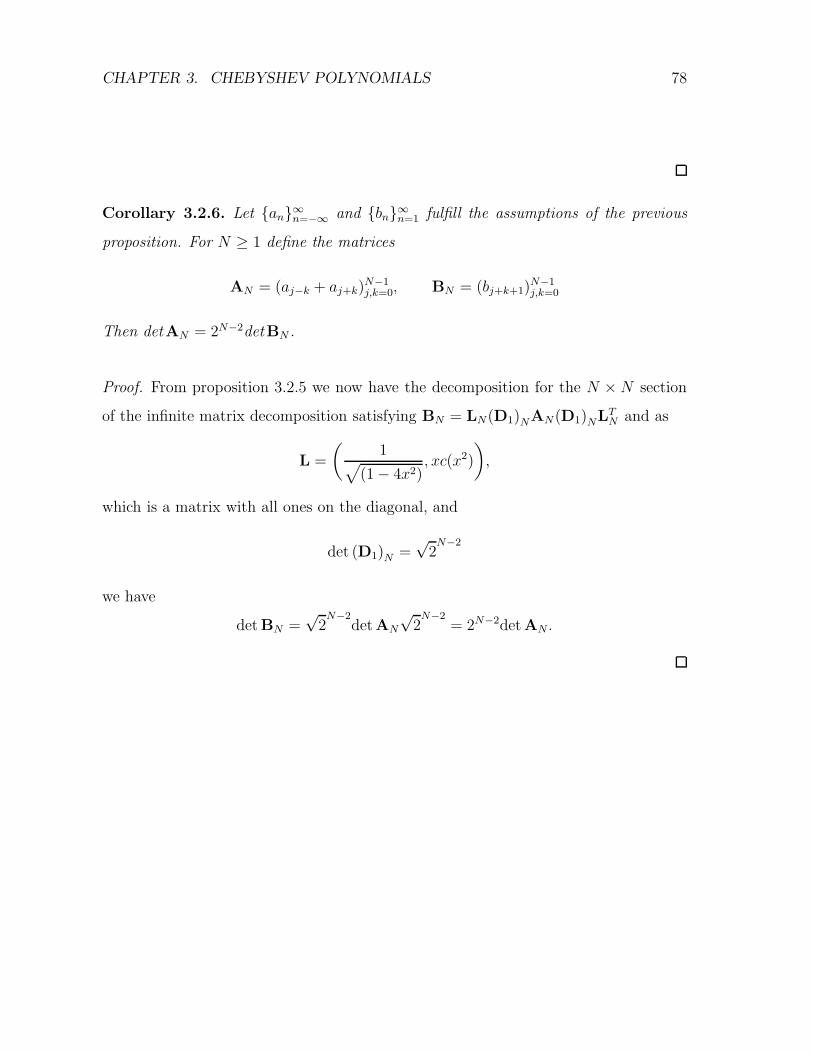
CHAPTER 3. CHEBYSHEV POLYNOMIALS 78
Corollary 3.2.6. Let {an}∞n=−∞ and {bn}∞n=1 fulfill the assumptions of the previous
proposition. For N ≥ 1 define the matrices
AN = (aj−k + aj+k)N−1j,k=0, BN = (bj+k+1)
N−1j,k=0
Then det AN = 2N−2det BN .
Proof. From proposition 3.2.5 we now have the decomposition for the N × N section
of the infinite matrix decomposition satisfying BN = LN(D1)NAN(D1)NLTN and as
L =
(
1√
(1 − 4x2), xc(x2)
)
,
which is a matrix with all ones on the diagonal, and
det (D1)N =√
2N−2
we have
det BN =√
2N−2
det AN
√2N−2
= 2N−2det AN .

Chapter 4
Properties of subgroups of the
Riordan group
In this chapter we look at the form of Stieltjes matrices of certain subgroups of theRiordan group. The subgroups we concern ourselves with in this section [120] are
• The Appell subgroup,
– Ordinary Appell subgroup:(
g(x), x)
– Exponential Appell subgroup:[
g(x), x]
• The Asssociated subgroup,
– Ordinary Asssociated subgroup:(
1, g(x))
– Exponential Asssociated subgroup:[
1, g(x)]
• The Bell subgroup
– Ordinary Bell subgroup:
(
g(x)
x, g(x)
)
– Exponential Bell subgroup:
[
ddx
g(x), g(x)
]
=[
h(x),∫
h(x)]
79

CHAPTER 4. PROPERTIES OF SUBGROUPS OF THE RIORDAN GROUP 80
• Hitting-time subgroup
– Ordinary Hitting-time subgroup:
(
x ddx
g(x)
g(x), g(x)
)
4.1 The Appell subgroup
4.1.1 The ordinary Appell subgroup
Riordan arrays in the Appell subgroup have the form (g(x), x) with inverse(
1g(x)
, x)
and they satisfy the group law as
(g(x), x) · (f(x), x) = (g(x)f(x), x).
We recall from [37] that given a Riordan array A = (g(x), f(x)), its Stieltjes (produc-tion) matrix P will be of the form
P =
ξ0 α0 0 0 0 0 . . .ξ1 α1 α0 0 0 0 . . .ξ2 α2 α1 α0 0 0 . . .ξ3 α3 α2 α1 α0 0 . . .ξ4 α4 α3 α2 α1 α0 . . .ξ5 α5 α4 α3 α2 α1 . . ....
......
......
.... . .
whereA(x) =
x
f(x),
and
Z(x) =1
f(x)
(
1 − 1
g(f(x))
)
,
where A(x) is the g.f. of α0, α1, . . . and Z(x) is the g.f. of the first column of P , thatis, of ξ0, ξ1, . . ..

CHAPTER 4. PROPERTIES OF SUBGROUPS OF THE RIORDAN GROUP 81
Proposition 4.1.1. Let A = (g(x), x) be a member of the Appell subgroup of the
Riordan group. Then its Stieltjes (production) matrix P is given by
P =
ξ0 1 0 0 0 0 . . .
ξ1 0 1 0 0 0 . . .
ξ2 0 0 1 0 0 . . .
ξ3 0 0 0 1 0 . . .
ξ4 0 0 0 0 1 . . .
ξ5 0 0 0 0 0 . . ....
......
......
.... . .
where
A(x) = x and Z(x) =1
x
(
1 − 1
g(x)
)
. (4.1)
Proof. We have f(x) = x and hence f(x) = x = x. Thus
A(x) =x
f(x)=
x
x= 1.
Also
Z(x) =1
f(x)
(
1 − 1
g(f(x))
)
=1
x
(
1 − 1
g(x)
)
.
Corollary 4.1.2. Let P be the Stieltjes matrix of the Appell group element (g(x), x).
Then
[xn]Z(x) =
n∑
k=0
[xk]1
g(x)[xn−k+1]g(x),
where Z(x) is the g.f. of the first column of P .

CHAPTER 4. PROPERTIES OF SUBGROUPS OF THE RIORDAN GROUP 82
Proof. By the above, we have
Z(x) =1
x
(
1 − 1
g(x)
)
=1
g(x)
g(x) − 1
x.
Hence
[xn]Z(x) = [xn]1
g(x)
g(x) − 1
x
=n∑
k=0
[xk]1
g(x)[xn−k]
g(x) − 1
x
=n∑
k=0
[xk]1
g(x)[xn−k+1](g(x) − 1)
=
n∑
k=0
[xk]1
g(x)([xn−k+1]g(x) − 0n−k+1)
=
n∑
k=0
[xk]1
g(x)[xn−k+1]g(x),
since there is a contribution from 0n−k+1 only when k = n + 1.
Corollary 4.1.3. The tridiagonal Stieltjes matrices corresponding to Riordan arrays
from the ordinary Appell subgroup have generating functions
A(x) = 1, Z(x) = β + αx
Proof. Riordan arrays from the Appell subgroup with corresponding tridiagonal ma-
trices have the form(
1
1 − βx− αx2, x
)
with inverse
(1 − βx− αx2, x).
Applying eq. (4.1) gives the result.

CHAPTER 4. PROPERTIES OF SUBGROUPS OF THE RIORDAN GROUP 83
Example. The Riordan array L from the Appell subgroup with
g(x) =1
1 − x−x2
1 − x−2x2
1 − x−3x2
1 − x− 4x2. . .
where g(x) is the g.f. for the Young tableaux numbers. L satisfies the matrix equation
LS = L where the first few rows expand as
1 0 0 0 0 0 . . .
1 1 0 0 0 0 . . .
2 1 1 0 0 0 . . .
4 2 1 1 0 0 . . .
10 4 2 1 1 0 . . .
26 10 4 2 1 1 . . ....
......
......
.... . .
1 1 0 0 0 0 . . .
1 0 1 0 0 0 . . .
1 0 0 1 0 0 . . .
3 0 0 0 1 0 . . .
7 0 0 0 0 1 . . .
23 0 0 0 0 0 . . ....
......
......
.... . .
=
1 1 0 0 0 0 . . .
2 1 1 0 0 0 . . .
4 2 1 1 0 0 . . .
10 4 2 1 1 0 . . .
26 10 4 2 1 1 . . .
76 26 10 4 2 1 . . ....
......
......
.... . . .
Z(x) generates the sequence which counts the number of indecomposable involutions of
length n [124](A140456).
Example. The Riordan array L from the Appell subgroup with
g(x) =1
1 − x−x2
1 − 2x−2x2
1 − 3x−3x2
1 − 4x− 4x2. . .

CHAPTER 4. PROPERTIES OF SUBGROUPS OF THE RIORDAN GROUP 84
where g(x) is the g.f. for the Bell numbers. L satisfies the matrix equation LS = L
where the first few rows expand as
1 0 0 0 0 0 . . .
1 1 0 0 0 0 . . .
2 1 1 0 0 0 . . .
5 2 1 1 0 0 . . .
15 5 2 1 1 0 . . .
52 15 5 2 1 1 . . ....
......
......
.... . .
1 1 0 0 0 0 . . .
1 0 1 0 0 0 . . .
1 0 0 1 0 0 . . .
2 0 0 0 1 0 . . .
6 0 0 0 0 1 . . .
22 0 0 0 0 0 . . ....
......
......
.... . .
=
1 1 0 0 0 0 . . .
2 1 1 0 0 0 . . .
5 2 1 1 0 0 . . .
15 5 2 1 1 0 . . .
52 15 5 2 1 1 . . .
203 52 15 5 2 1 . . ....
......
......
.... . . .
Here Z(x) generates the sequence which counts the number of set partitions of n which
do not have a proper subset of parts with a union equal to a subset(number of irreducible
set partitions of size n) [124] (A074664).
4.1.2 Exponential Appell subgroup
We now consider the exponential Appell subgroup, comprised of arrays of the form
[g(x), x].
We recall that for an exponential Riordan array [g(x), f(x)], its Stieltjes (production)matrix will have bivariate g.f.
exy(c(x) + r(x)y), (4.2)
where
c(x) =g′(f(x))
g(f(x)),
andr(x) = f ′(f(x)).
For the exponential Appell subgroup, we then have

CHAPTER 4. PROPERTIES OF SUBGROUPS OF THE RIORDAN GROUP 85
Proposition 4.1.4. Let A = [g(x), x] be a member of the exponential Appell subgroup
of the exponential Riordan group. Then its Stieltjes (production) matrix P will have
bivariate g.f.
exy(
g′(x)
g(x)+ y
)
.
Proof. We have f(x) = x and hence f(x) = x and f ′(x) = 1. Thus r(x) = 1. Also, we
have
c(x) =g′(f(x))
g(f(x))=
g′(x)
g(x).
The result follows from eq. (4.2) .
Corollary 4.1.5. The e.g.f. of the first column of P is given by
g′(x)
g(x)=
d
dxln(g(x)). (4.3)
We note that for k ≤ n, the (n, k)-th element of P is given by(
n
k
)
ξn−k,
where the elements of the first column are
ξ0, ξ1, ξ2, . . . .
Corollary 4.1.6. The n-th element of the first column of P is given by
n!
n∑
k=0
[xk]1
g(x)[xn−k+1]g(x).
Proof. The first column of P has e.g.f. given by g′(x)g(x)
, thus its n-th element is given by
n![xn]g′(x)g(x)
. Now
[xn]g′(x)
g(x)=
n∑
k=0
[xk]1
g(x)[xn−k]g′(x)
=n∑
k=0
[xk]1
g(x)[xn−k+1]g(x).

CHAPTER 4. PROPERTIES OF SUBGROUPS OF THE RIORDAN GROUP 86
Corollary 4.1.7. Exponential Riordan arrays in the Appell subgroup with a corre-
sponding tridiagonal Stieltes matrices have the form
[e(βx+αx2/2), x] (4.4)
with inverse [e−(βx+αx2/2), x].
Proof. From eq. (4.3) we have
g(x)c(x) =d
dxg(x).
Expanding for Riordan arrays with corresponding tridiagonal Stieltjes matrices we then
have
g(x)(β + αx) =d
dxg(x).
Solving the differential equation gives
g(x) = e(βx+αx2/2).
The related Stieltjes matrix has first few entries
β 1 0 0 0 0 . . .
α β 1 0 0 0 . . .
0 2α β 1 0 0 . . .
0 0 3α β 1 0 . . .
0 0 0 4α β 1 . . .
0 0 0 0 5α β . . ....
......
......
.... . .
.
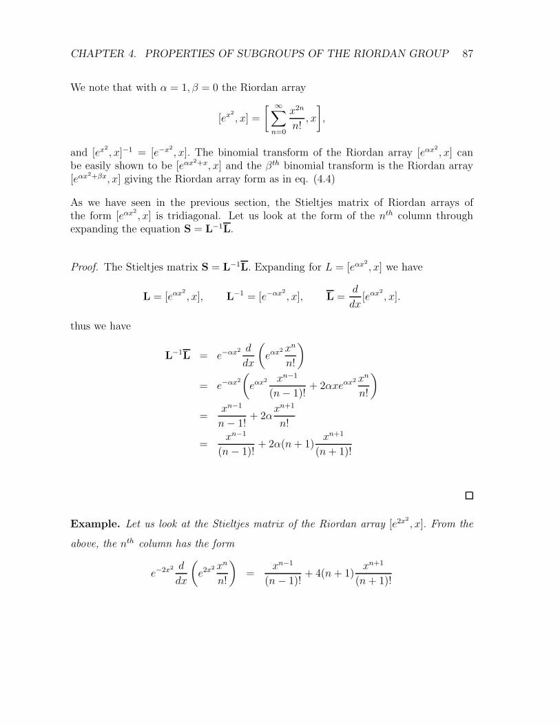
CHAPTER 4. PROPERTIES OF SUBGROUPS OF THE RIORDAN GROUP 87
We note that with α = 1, β = 0 the Riordan array
[ex2
, x] =
[ ∞∑
n=0
x2n
n!, x
]
,
and [ex2, x]−1 = [e−x2
, x]. The binomial transform of the Riordan array [eαx2, x] can
be easily shown to be [eαx2+x, x] and the βth binomial transform is the Riordan array
[eαx2+βx, x] giving the Riordan array form as in eq. (4.4)
As we have seen in the previous section, the Stieltjes matrix of Riordan arrays ofthe form [eαx
2, x] is tridiagonal. Let us look at the form of the nth column through
expanding the equation S = L−1L.
Proof. The Stieltjes matrix S = L−1L. Expanding for L = [eαx2, x] we have
L = [eαx2
, x], L−1 = [e−αx2
, x], L =d
dx[eαx
2
, x].
thus we have
L−1L = e−αx2 d
dx
(
eαx2 xn
n!
)
= e−αx2
(
eαx2 xn−1
(n− 1)!+ 2αxeαx
2 xn
n!
)
=xn−1
n− 1!+ 2α
xn+1
n!
=xn−1
(n− 1)!+ 2α(n + 1)
xn+1
(n + 1)!
Example. Let us look at the Stieltjes matrix of the Riordan array [e2x2, x]. From the
above, the nth column has the form
e−2x2 d
dx
(
e2x2 xn
n!
)
=xn−1
(n− 1)!+ 4(n + 1)
xn+1
(n + 1)!

CHAPTER 4. PROPERTIES OF SUBGROUPS OF THE RIORDAN GROUP 88
which in matrix notation is
1 0 0 0 . . .
0 1 0 0 . . .
−4 0 1 0 . . .
0 −12 0 1 . . .
48 0 −24 0 . . ....
......
.... . .
0 1 0 0 . . .
4 0 1 0 . . .
0 12 0 1 . . .
48 0 24 0 . . .
0 240 0 40 . . ....
......
.... . .
=
0 1 0 0 . . .
4 0 1 0 . . .
0 8 0 1 . . .
0 0 12 0 . . .
0 0 0 16 . . ....
......
.... . .
.
Proposition 4.1.8. The Stieltjes matrix of successive Binomial transforms of [e−αx2, x]
has nth columnxn−1
(n− 1)!+ β
xn
n!+ 2α(n + 1)
xn+1
n!.
Proof.
e−αx2+βx d
dx
(
eαx2+βxx
n
n!
)
= e−αx2+βx
(
eαx2+βx xn−1
(n− 1)!+ 2αxeαx
2+βxxn
n!+ βeαx
2+βxxn
n!
)
=xn−1
(n− 1)!+ β
xn
n!+ 2α(n + 1)
xn+1
n!.
Example. Once again with α = 1/2, the nth column of the Stieltjes matrix correspond-
ing to the βth binomial transform of the Riordan array [e−x2
2 , x] is
e−βx−x2
2d
dx
(
eβx+x2
2xn
n!
)
= e−βx−x2
2
(
ex2
2+βxxn+1
n!+
ex2
2+βxβxn
n!+
ex2
2+βxxn−1
(n− 1)!
)
=xn+1
n!+
βxn
n!+
xn−1
(n− 1)!
=xn−1
(n− 1)!+
βxn
n!+
(n + 1)xn+1
(n + 1)!.

CHAPTER 4. PROPERTIES OF SUBGROUPS OF THE RIORDAN GROUP 89
Thus L−1L is the tridiagonal matrix
S =
β 1 0 0 0 0
1 β 1 0 0 0
0 2 β 1 0 0
0 0 3 β 1 0
0 0 0 4 β 1
0 0 0 0 5. . .
.
Example.
eβx+x2
2 =
∞∑
n=0
βxn
n!
∞∑
m=0
x2m
2mm!.
With β = 0 we have
L =
[ ∞∑
n=0
x2n
2nn!, x
]
=
1 0 0 0 0 0
0 1 0 0 0 0
1 0 1 0 0 0
0 3 0 1 0 0
3 0 6 0 1 0
0 3 0 10 0 1
, (A001147)
L−1 =
[ ∞∑
n=0
x2n
2nn!, x
]−1
=
[ ∞∑
n=0
(−1)nx2n
2nn!, x
]
=
1 0 0 0 0 0
0 1 0 0 0 0
−1 0 1 0 0 0
0 −3 0 1 0 0
3 0 −6 0 1 0
0 3 0 −10 0 1
.

CHAPTER 4. PROPERTIES OF SUBGROUPS OF THE RIORDAN GROUP 90
4.2 The associated subgroup
4.2.1 Ordinary associated subgroup
Riordan arrays (1, xg(x)) form the associated subgroup. They satisfy the group lawwhere
(1, xg(x))(1, xf(x)) = (1, xf(xg(x)))
and have inverse Riordan arrays of the form (1, xg(x)).
Proposition 4.2.1. Let A = (1, xg(x)) be a member of the associated subgroup of the
Riordan group. Then its Stieltjes (production) matrix P is given by
P =
0 α0 0 0 0 0 . . .
0 α1 α0 0 0 0 . . .
0 α2 α1 α0 0 0 . . .
0 α3 α2 α1 α0 0 . . .
0 α4 α3 α2 α1 α0 . . .
0 α5 α4 α3 α2 α1 . . ....
......
......
.... . .
where
A(x) =x
xg(x)and Z(x) = 0. (4.5)
Proof. From [36] we have
A(x) =x
f(x)=
x
xg(x).
Also
Z(x) =1
f(x)
(
1 − 1
g(f(x))
)
=1
xg(x)
(
1 − 1
1
)
= 0.

CHAPTER 4. PROPERTIES OF SUBGROUPS OF THE RIORDAN GROUP 91
Corollary 4.2.2. Tridiagonal Stieltjes matrices relating to Riordan arrays from the
ordinary associated subgroup have generating functions
A(x) = 1 + βx + αx2, Z(x) = 0.
Proof. Riordan arrays from the Appell subgroup with corresponding tridiagonal ma-
trices have the form(
1,x
1 − βx− αx(xg(x))
)
sox
xg(x)= 1 + βx + αx2.
Applying eq. (4.5) gives the result.
Example.
1 0 0 0 0 0 . . .
0 1 0 0 0 0 . . .
0 1 1 0 0 0 . . .
0 2 2 1 0 0 . . .
0 5 5 3 1 0 . . .
0 15 14 9 4 1 . . ....
......
......
.... . .
0 1 0 0 0 0 . . .
0 1 1 0 0 0 . . .
0 1 1 1 0 0 . . .
0 1 1 1 1 0 . . .
0 2 1 1 1 1 . . .
0 6 2 1 1 1 . . ....
......
......
.... . .
=
0 1 0 0 0 0 . . .
0 1 1 0 0 0 . . .
0 2 2 1 0 0 . . .
0 5 5 3 1 0 . . .
0 15 14 9 4 1 . . .
0 52 44 28 14 5 . . ....
......
......
.... . .
.
The sequence A(x) counts the number of connected partitions of n (A099947) [124].

CHAPTER 4. PROPERTIES OF SUBGROUPS OF THE RIORDAN GROUP 92
Example.
1 0 0 0 0 0 . . .
0 1 0 0 0 0 . . .
0 1 1 0 0 0 . . .
0 2 2 1 0 0 . . .
0 4 5 3 1 0 . . .
0 10 12 9 4 1 . . .
0 26 32 25 14 1 . . ....
......
......
.... . .
0 1 0 0 0 0 . . .
0 1 1 0 0 0 . . .
0 1 1 1 0 0 . . .
0 0 1 1 1 0 . . .
0 1 0 1 1 1 . . .
0 0 1 0 1 1 . . .
0 4 0 1 0 1 . . ....
......
......
.... . .
=
0 1 0 0 0 0 . . .
0 1 1 0 0 0 . . .
0 2 2 1 0 0 . . .
0 4 5 3 1 0 . . .
0 10 12 9 4 1 . . .
0 26 32 25 14 5 . . ....
......
......
.... . . ,
.
The sequence A(x) counts the number of irreducible diagrams with 2n nodes (A172395) [124].
4.2.2 Exponential associated subgroup
Proposition 4.2.3. Let A = [1, f(x)] be a member of the exponential associated sub-
group of the exponential Riordan group. Then its Stieltjes (production) matrix P will
have bivariate g.f.
exy(
f ′(f(x))y)
.
Proof. We have g(x) = 1 and hence c(x) = 0. Also, we have
r(x) = f ′(f(x)).
The result follows from eq. (4.2).

CHAPTER 4. PROPERTIES OF SUBGROUPS OF THE RIORDAN GROUP 93
The first few rows of tridiagonal Stieltjes matrices in this subgroup expand as
0 1 0 0 0 0 . . .0 β 1 0 0 0 . . .0 α 2β 1 0 0 . . .0 0 3α 3β 1 0 . . .0 0 0 6α 4β 1 . . .0 0 0 0 10α 5β . . ....
......
......
.... . .
with general element
a(n,n) =nan−1,n−1
n− 1, a(n+1,n) =
(n + 1)(an,n−1)
n− 1.
By expanding the second column of the matrix equation LS = L we see that generatingfunctions from the associated subgroup with tridiagonal Stieltjes matrices satisfy thedifferential equation
d
dxg(x) = 1 + βg(x) +
αg(x)2
2.
Solving the ordinary differential equation gives
g(x) = −−b +
√b2 − 2ctanh
(
12x√b2 − 2c− Arctanh
(
b√b2−2c
))
c.
Example. We take a member of the associated subgroup, [1, g(x)] where the related
Stieltjes matrix has first few rows
0 1 0 0 0 0 . . .
0 1 1 0 0 0 . . .
0 1 2 1 0 0 . . .
0 0 3 3 1 0 . . .
0 0 0 6 4 1 . . .
0 0 0 0 10 5 . . ....
......
......
.... . .
.

CHAPTER 4. PROPERTIES OF SUBGROUPS OF THE RIORDAN GROUP 94
Expanding the first column of the matrix equation L = LS, the e.g.f. of the related
Riordan matrix of the associated subgroup satisfies the equation
d
dxg(x) = 1 + g(x) + g(x)2/2.
Solving gives
xg(x) = −1 + tan
(
x
2+
π
4
)
.
Expanding for the first few terms we have 1, 1, 2, 5, 16, 61 . . . (A000111).
Example. Again, we take a member of the associated subgroup where g(x) is an e.g.f.
and the related Stieltjes matrix has first few rows
0 1 0 0 0 0 . . .
0 0 1 0 0 0 . . .
0 1 0 1 0 0 . . .
0 0 3 0 1 0 . . .
0 0 0 6 0 1 . . .
0 0 0 0 10 0 . . ....
......
......
.... . .
.
Expanding the first column of the matrix equation L = LS, the e.g.f. of the related
Riordan matrix of the associated subgroup satisfies the equation
d
dxg(x) = 1 + g(x)2/2,
and solving gives
xg(x) =√
2tan( x√
2
)
.
Expanding for the first few terms we have 1, 1, 4, 34, 496, . . . which is the aerated se-
quence of reduced tangent numbers(A002105).

CHAPTER 4. PROPERTIES OF SUBGROUPS OF THE RIORDAN GROUP 95
4.3 The Bell subgroup
4.3.1 Ordinary Bell subgroup
Elements of the Bell subgroup have the form (g(x), xg(x)) and satisfy the group law as
(g(x), xg(x)) · (f(x), xf(x)) =
(
g(x)f(xg(x)), xf(xg(x))
)
.
The Bell subgroup decomposes into the associated and Appell subgroups as
(g(x), xg(x)) = (g(x), x) · (1, xg(x)).
Now, before we continue we introduce the following proposition which we will be of useto us in the section below.
Proposition 4.3.1.x
g(xg(x))= xg(x) (4.6)
Proof.
(g(x), xg(x))(1, x) = (g(x), xg(x))
so we have
(1, x) = (g(x), xg(x))−1(
g(x), xg(x))
=
(
1
g(xg(x)), xg(x)
)
(g(x), xg(x))
=
(
1
g(xg(x))g(xg(x)), xg(x)g(xg(x))
)
= (1, xg(x)g(xg(x)))
so
xg(x) =x
g(xg(x))

CHAPTER 4. PROPERTIES OF SUBGROUPS OF THE RIORDAN GROUP 96
Proposition 4.3.2. Let A = (g(x), xg(x)) be a member of the Bell subgroup of the
Riordan group. Then its Stieltjes (production) matrix P is given by
P =
ξ0 α0 0 0 0 0 . . .
ξ1 α1 α0 0 0 0 . . .
ξ2 α2 α1 α0 0 0 . . .
ξ3 α3 α2 α1 α0 0 . . .
ξ4 α4 α3 α2 α1 α0 . . .
ξ5 α5 α4 α3 α2 α1 . . ....
......
......
.... . .
where
A(x) =x
xg(x)and Z(x) =
1
xg(x)− 1. (4.7)
Proof. We have f(x) = xg(x) and hence f(x) = xg(x). Thus
A(x) =x
xg(x).
Also
Z(x) =1
xg(x)
(
1 − 1
g(xg(x))
)
=1
xg(x)
(
1 − xg(x)
x
)
=1
xg(x)− 1
x.
Corollary 4.3.3. The tridiagonal Stieltjes matrices corresponding to Riordan arrays
from the ordinary Bell subgroup have generating functions
A(x) = 1 + βx + αx2, Z(x) = β + αx

CHAPTER 4. PROPERTIES OF SUBGROUPS OF THE RIORDAN GROUP 97
Proof. Riordan arrays from the Bell subgroup with corresponding tridiagonal matrices
have the form(
1
1 − βx− αx2g(x),
x
1 − βx− αx2g(x)
)
with
(
1
1 − βx− αx2g(x),
x
1 − βx− αx2g(x)
)−1
=
(
1
1 + βx + αx2,
x
1 + βx + αx2
)
.
Thus
xg(x) =x
1 + βx + αx2.
Applying eq. (4.7) gives the result.
4.3.2 Exponential Bell subgroup
For the exponential Bell subgroup we have Riordan arrays of the form [g(x),∫
g(x)],or alternatively [ d
dxh(x), h(x)].
Proposition 4.3.4. Let A = [g(x),∫
g(x)] be a member of the exponential Bell sub-
group of the exponential Riordan group. Then its Stieltjes (production) matrix P will
have bivariate g.f.
exy
(
g′(∫
g(x))
g(∫
g(x))+ g(
∫
g(x))y
)
.
Proof.
c(x) =g′(∫
g(x))
g(∫
g(x)),
and
r(x) = f ′(f(x)) = g(
∫
g(x)).
The result follows from eq. (4.2).

CHAPTER 4. PROPERTIES OF SUBGROUPS OF THE RIORDAN GROUP 98
Now once again, we look at the form of the related tridiagonal Stieltjes matrices byequating columns of LS = L, and we get the related tridiagonal Stieltjes matrices withfirst few elements
γ 1 0 0 0 . . .δ β 1 0 0 . . .0 α 2β − γ 1 0 . . .0 0 3α− 3δ 3β − 2γ 1 . . .0 0 0 2(3α− 4δ) 4β − 3γ . . ....
......
......
. . .
,
with (n, n)th and (n, n− 1)th entries
ann =nan−1,n−1 − γ
n− 1, an+1,n =
(n + 1)(an,n−1 − δ)
(n− 1).
Expanding the first column of the equation LS = L we have the equation
γg(x) + δ
∫
g(x) dx =d
dxg(x) (4.8)
Let us look at an example.
Example. With γ, δ equal to one we have the e.g.f. of the form
1
1 − sin x
with the sequence of coefficients having first few terms 1, 1, 2, 5, 16, 61 . . . which is the
sequence of the Euler numbers(A000111) and also counts the number of alternating
permutations on n letters. We have
S =
1 1 0 0 0 . . .
1 2 1 0 0 . . .
0 3 3 1 0 . . .
0 0 6 4 1 . . .
0 0 0 10 5 . . ....
......
......
. . .
.
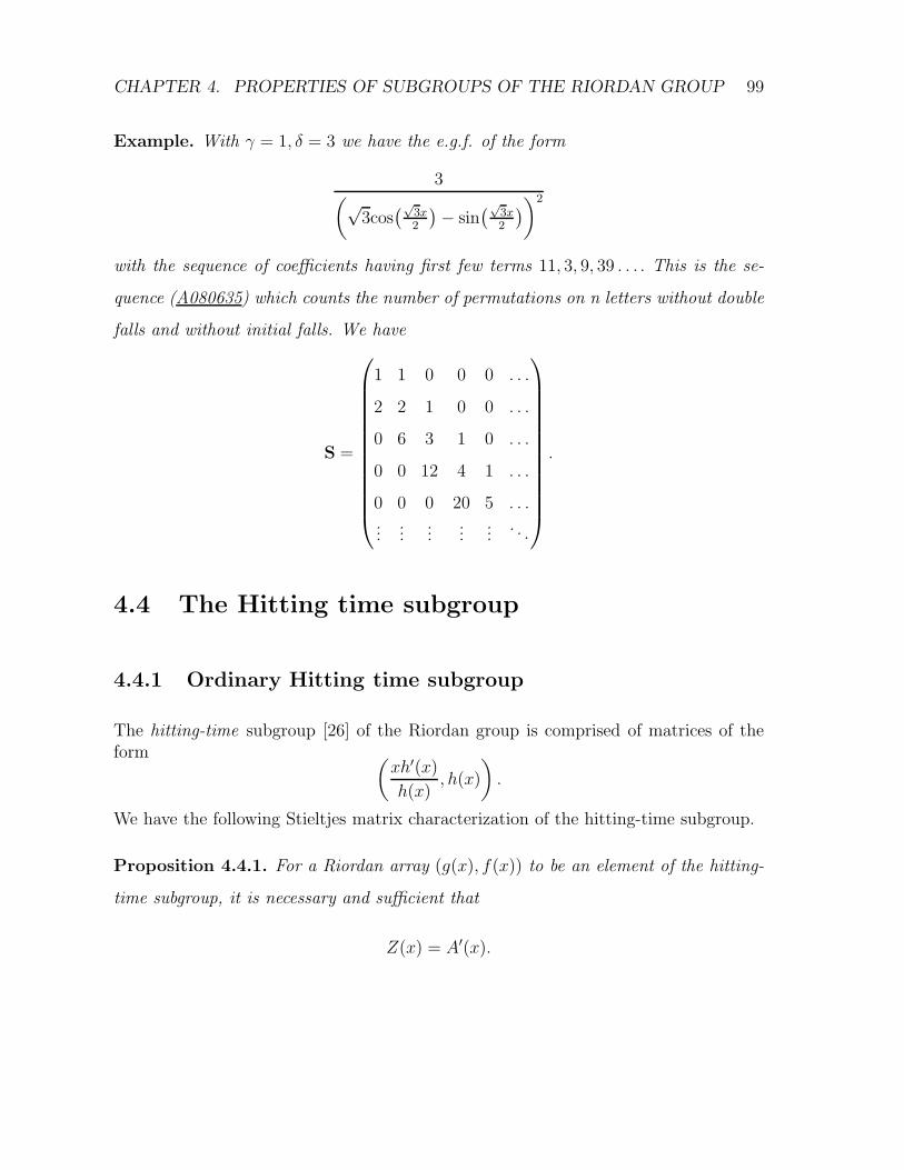
CHAPTER 4. PROPERTIES OF SUBGROUPS OF THE RIORDAN GROUP 99
Example. With γ = 1, δ = 3 we have the e.g.f. of the form
3(√
3cos(
√3x2
)
− sin(
√3x2
)
)2
with the sequence of coefficients having first few terms 11, 3, 9, 39 . . . . This is the se-
quence (A080635) which counts the number of permutations on n letters without double
falls and without initial falls. We have
S =
1 1 0 0 0 . . .
2 2 1 0 0 . . .
0 6 3 1 0 . . .
0 0 12 4 1 . . .
0 0 0 20 5 . . ....
......
......
. . .
.
4.4 The Hitting time subgroup
4.4.1 Ordinary Hitting time subgroup
The hitting-time subgroup [26] of the Riordan group is comprised of matrices of theform
(
xh′(x)
h(x), h(x)
)
.
We have the following Stieltjes matrix characterization of the hitting-time subgroup.
Proposition 4.4.1. For a Riordan array (g(x), f(x)) to be an element of the hitting-
time subgroup, it is necessary and sufficient that
Z(x) = A′(x).

CHAPTER 4. PROPERTIES OF SUBGROUPS OF THE RIORDAN GROUP 100
Proof. We show first that the condition is necessary. Thus let
A = (g(x), f(x)) =
(
xh′(x)
h(x), h(x)
)
.
Then
A(x) =x
f(x)=
x
h(x).
Thus
h(x) =x
A(x)
and1
h(x)=
A(x)
x.
Now
Z(x) =1
h(x)
(
1 − 1
g(h(x))
)
=1
h(x)
1 − 1h(x)h′(h(x))
h(h(x))
=1
h(x)
(
1 − x
h(x)h′(h(x))
)
=1
h(x)
(
1 − A(x)
h′(h(x))
)
=A(x)
x
(
1 − A(x)
h′(h(x))
)
.
Now differentiating the identity h(f(x)) = x with respect to x gives
h′(h(x))(h)′(x) = 1
and so
h′(h(x)) =1
(h)′(x).
Now since
h(x) =x
A(x)

CHAPTER 4. PROPERTIES OF SUBGROUPS OF THE RIORDAN GROUP 101
we have
(h)′(x) =A(x) − xA′(x)
A(x)2,
and so we get
Z(x) =A(x)
x
(
1 −A(x)A(x) − xA′(x)
A(x)2
)
=A(x)
x− A(x)2
x
A(x) − xA′(x)
A(x)2
=A(x)
x− A(x)
x+
xA′(x)
x
= A′(x).
Thus let
Z(x) = A′(x),
where
f(x) =x
A(x)or A(x) =
x
f(x).
Now
Z(x) =1
f(x)
(
1 − 1
g(f(x))
)
.
Thus
g(f(x)) =1
1 − f(x)Z(x)
and hence
g(x) =1
1 − xZ(f(x)).

CHAPTER 4. PROPERTIES OF SUBGROUPS OF THE RIORDAN GROUP 102
From this we infer that
g(x) =1
1 − xZ(f(x))
=1
1 − xA′(f(x))
=1
1 − x f(f(x))−f(x)(f )′(f(x))
f(f(x))2
=1
1 − xx−f(x)(f )′(f(x))x2
=1
1 − 1 + f(x)(f )′(f(x))x
=x
f(x)(f)′(f(x))
=xf ′(f(f(x)))
f(x)
=xf ′(x)
f(x).
Corollary 4.4.2. Riordan arrays with tridiagonal Stieltjes matrices which are elements
of the hitting time subgroup have the form
(
1
1 − βx− 2αg(x),
x
1 − βx− αg(x)
)
.
Proof. Let
g(x) =x
1 − βx− αg(x)= −1 − αx−
√
x2(α2 − 4β) − 2αx + 1
2βx
soxg′(x)
g(x)=
1√
x2(α2 − 4βx) − 2αx + 1=
x
1 − βx− 2αg(x)

CHAPTER 4. PROPERTIES OF SUBGROUPS OF THE RIORDAN GROUP 103
Example.
S =
1 1 0 0 . . .
2 1 1 0 . . .
0 1 1 0 . . .
0 0 1 1 . . .
0 0 0 1 . . ....
......
.... . .
The related Riordan array has the form
(f(x), g(x)) =
(
1
1 − x− 2xg(x),
x
1 − x− xg(x)
)
.

Chapter 5
Lattice paths and Riordan arrays
In this chapter we will study the well-known Motzkin and Lukasiewicz paths. Motzkinpaths have well established links to orthogonal polynomials; as we have seen in [56],the entries of the tridiagonal Stieltjes matrix represent the weights of the possible stepsin the Motzkin paths. We begin this chapter by introducing lattice paths, particularlyMotzkin and Lukasiewicz paths which we study through the medium of Riordan arrays.We give a constructive proof of how Riordan arrays with non-tridiagonal Stieltjes ma-trices relate to Lukasiewicz paths. We then develop these paths through the mediumof Riordan arrays.
Let us recall the definition of a lattice path which we introduced in section 2.5. Alattice path [79] is a sequence of points in the integer lattice Z2. A pair of consecutivepoints is called a step of the path. A valuation is a function on the set of possible stepsof Z2 × Z2. A valuation of a path is the product of the valuations of its steps. Weconcern ourselves with two types of paths, Motzkin paths and Lukasiewicz paths [151],which are defined as follows
Definition 5.0.1. A Motzkin path [78] π = (π(0), π(1), . . . , π(n)), of length n, is a
lattice path starting at (0, 0) and ending at (n, 0) that satisfies the following conditions
1. The elementary steps can be north-east(N-E), east(E) and south-east(S-E).
104

CHAPTER 5. LATTICE PATHS AND RIORDAN ARRAYS 105
2. Steps never go below the x axis.
Dyck paths are Motzkin paths without the possibility of an East(E) step.
Definition 5.0.2. A Lukasiewicz path [78] π = (π(0), π(1), . . . , π(n)), of length n, is a
lattice path starting at (0, 0) and ending at (n, 0) that satisfies the following conditions
1. The elementary steps can be north-east(N-E) and east(E) as those in Motzkin
paths.
2. South-east(S-E) steps from level k can fall to any level above or on the x axis,
and are denoted as αn,k, where n is the length of the south-east step and k is the
level where the step ends.
3. Steps never go below the x axis.
Finally, we introduce the Schroder paths, as we will encounter these paths at a laterstage
Definition 5.0.3. A Schroder path π = (π(0), π(1), . . . , π(2n)), of semilength n, is a
lattice path starting at (0, 0) and ending at (2n, 0) that satisfies the following conditions
1. The elementary steps can be north-east(N-E), east(E) and south-east(S-E) with
easterly steps begin twice the length of the north-easterly and south-easterly steps.
2. Steps never go below the x axis.
5.1 Motzkin, Schroder and Lukasiewicz paths
Firstly, let us illustrate the construction of the (n+ 1)th row of the Riordan array. The(m,n)th entry of the Riordan array is lm,n where m is the length of the path and n is

CHAPTER 5. LATTICE PATHS AND RIORDAN ARRAYS 106
the height of the final position of the last step. In [56], we see that the entries of thetridiagonal Stieltjes matrix represent the weights of the possible steps in the Motzkinpaths. From the 0th column calculated from the Stieltjes equation L = LS, as
ln+1,0 = ln,0β0,0 + ln,1α1,0
so clearly, ln+1,0 is calculated from ln,0 with a level step at the zero level, and ln,1, withan added south-east step, α1,0 so for m > 0,
ln+1,m = ln,m−1 + ln,mβm,m + ln,m+1αm+1,m. (5.1)
From (5.1) we see the paths contributing to ln+1,m are as follows
• Paths of length n finishing at level m− 1(ln,m−1), adding one N-E step of weight1.
• Paths of length n finishing at level m(ln,m), adding one E step of weight βm,m.
• Paths of length n finishing at level m + 1(ln,m+1), adding one S-E step of weightαm+1,m.
Now, consider a Riordan array with non-tridiagonl Stieltjes matrix,
β0,0 1 0 0 0 0 . . .α1,0 β1,1 1 0 0 0 . . .α2,0 α2,1 β2,2 1 0 0 . . .α3,0 α3,1 α3,2 β3,3 1 0 . . .α4,0 α4,1 α4,2 α4,3 β4,4 1 . . .α5,0 α5,1 α5,2 α5,3 α5,4 β5,5 . . .
......
......
......
. . .
. (5.2)
Here we have the possibility of any length of south-easterly step, so for the 0th columnwe have
ln+1,0 = ln,0β0,0 + ln,1α1,0 + ln,2α2,0 + · · · + ln,nαn,0,
and for any m we have
ln+1,m = ln,m−1 + ln,mβm,m + ln,m+1αm+1,m + ln,m+2αm+2,m + · · · + ln,nαn,m. (5.3)
From (5.3) we see the paths contributing to the lthn+1,m Lukasiewicz path are as follows

CHAPTER 5. LATTICE PATHS AND RIORDAN ARRAYS 107
• Paths of length n finishing at level m− 1(ln,m−1), adding one N-E step of weight1.
• Paths of length n finishing at level m(ln,m), adding one E step βm,m.
• Paths of length n finishing at level m + 1(ln,m+1), adding an αm+1,m Lukasiewiczstep.
• Paths of length n finishing at level m + 1(ln,m+2), adding an αm+2,m Lukasiewiczstep.
...
• Paths of length n finishing at level m+ 1(ln,n), adding an αn,m Lukasiewicz step.
Note that in this chapter we adopt the following notation for our Motzkin and Lukasiewiczpaths. (α, β)-Motzkin path and (α, β)- Lukasiewicz paths can be viewed as colouredMotzkin/ Lukasiewicz paths in the sense that there are β colours for each level step andα colours for each down step.
5.1.1 The binomial transform of lattice paths
The Binomial transform of generating functions has been of interest to us in previouschapters. We now look at the effect of the binomial transform of a Riordan array interms of steps of Motzkin paths. Let us first look at Dyck paths, which have no levelsteps and then introduce the level steps via the Binomial transform.
The sequence that counts Dyck paths has g.f.
g(x) =1 −
√
(1 − 4αx2)
2αx2.
The general Riordan array corresponding to Dyck paths has the form
(
1 −√
(1 − 4αx2)
2αx2,1 −
√
(1 − 4αx2)
2αx
)
.

CHAPTER 5. LATTICE PATHS AND RIORDAN ARRAYS 108
When α = 1, this is the sequence of aerated Catalan numbers. The g.f. of the Dyckpaths has continued fraction expansion
1
1 − αx2
1 − αx2
1 − αx2
. . .
.
Now, the βth binomial transform matrix has first few rows
1 0 0 0 . . .β 1 0 0 . . .β2 2β 1 0 . . .β3 3β2 3β 1 . . .β4 4β3 6β2 4β . . ....
......
.... . .
=
(
1
1 − βx,
x
1 − βx
)
.
Calculating the binomial transform of (g(x), xg(x)) we have
(
1
1 − βx,
x
1 − βx
)(
1 −√
(1 − 4αx2)
2αx2,
1 −√
(1 − 4αx2)
2αx
)
resulting in the Riordan array with first column having the g.f.
1 −√
(1 − 4α(
x1−βx
)2)
2α(
x1−βx
)2 ,
which has continued fraction expansion,
1
1 − βx− αx2
1 − βx− αx2
1 − βx− αx2
. . .
.
From the continued fraction expansion we have seen in [56], the binomial transformhas introduced the level steps in the Motzkin paths.

CHAPTER 5. LATTICE PATHS AND RIORDAN ARRAYS 109
Now, let us look at the contribution of the binomial matrix to each path in our Riordanarray. Let,
L =
a0,0 0 0 0 . . .a1,0 a1,1 0 0 . . .a2,0 a2,1 a2,2 0 . . .a3,0 a3,1 a3,2 a3,3 . . .a4,0 a4,1 a4,2 a4,3 . . .
......
......
. . .
.
Let us now look at the paths in the Riordan array after multiplication by the Binomialmatrix,
1 0 0 0 . . .β 1 0 0 . . .β2 2β 1 0 . . .β3 3β2 3β 1 . . .β4 4β3 6β2 4β . . .β5 5β4 10β3 10β2 . . ....
......
.... . .
a0,0 0 0 0 0 . . .a1,0 a1,1 0 0 0 . . .a2,0 a2,1 a2,2 0 0 . . .a3,0 a3,1 a3,2 a3,3 0 . . .a4,0 a4,1 a4,2 a4,3 a4,4 . . .a5,0 a5,1 a5,2 a5,3 a5,4 . . .
......
......
.... . .
.
We denote the elements in the Binomial transformed Riordan array, bl. We investigatethe contribution to one such element, bl5,0. From the matrix multiplication above wehave
bl5,0 =
(
5
5
)
β5a0,m +
(
5
4
)
β4a1,m +
(
5
3
)
β3a2,m +
(
5
2
)
β3a3,m +
(
5
1
)
βa4,m +
(
5
0
)
βa5,m
We can now see the effect of the binomial transform on each of the level steps thatcontribute to the new step bl5,0 :
•(
55
)
β5a0,0, is the Dyck path of length 0, with a choice of 1 place for the 5 levelsteps,
(
5
5
)
=
(
1
1
)(
4
4
)
,
with no choice of length of level paths as we are filling one position only.
• Now for(
54
)
β4a1,0, is the Dyck path of length 1, with a choice of 2 places for 4level steps, and choice for arranging the level steps giving,
(
5
4
)
=
(
2
1
)(
3
3
)
+
(
2
2
)(
3
2
)
.

CHAPTER 5. LATTICE PATHS AND RIORDAN ARRAYS 110
• Now for(
53
)
β3a2,0, the path is length 2 with a choice of 3 places for 3 level steps,and choice for arranging the level steps giving,
(
5
3
)
=
(
3
1
)(
2
2
)
+
(
3
2
)(
2
1
)
+
(
3
2
)(
2
0
)
.
• Now for(
52
)
β2a3,0, the path is length 3 with a choice of 4 places for 2 level steps,and choice for arranging the level steps giving
(
5
2
)
=
(
4
1
)(
1
1
)
+
(
4
2
)(
1
0
)
.
• Now for(
51
)
βa4,0, the path is length 4 with a choice of 5 places for 1 level steps,
(
5
1
)
=
(
5
1
)(
0
0
)
.
We illustrate the effect of the binomial transform in the table below. The red dotsrepresent the Motzkin path an,m where n is the path length and m is the level of thelast step. Note that as the paths may take on different forms, depending on m, thedots represent each of the N-E or S-E steps.

CHAPTER 5. LATTICE PATHS AND RIORDAN ARRAYS 111
a0,m(
11
)
a1,m(
21
)
(
22
)(
31
)
a2,m(
31
)
(
32
)(
21
)
(
33
)
a3,m(
41
)
(
42
)
a4,m(
51
)
Now, for any lattice path step and the binomial transform we have
(
n
m
)
βman−m =
min(m,n−m+1)∑
q=1
(
n−m + 1
q
)(
m− 1
m− q
)
βman−m
• For the path an−m we have n−m + 1 choices of positions for the m level steps,with m ≤ n.
• Now, we can choose q of these n−m + 1 positions to place the m level steps.

CHAPTER 5. LATTICE PATHS AND RIORDAN ARRAYS 112
• If we choose q of the n−m+ 1 positions to place the level steps, we now need tochoose the number of level steps to put at each of the q positions.
Example. Let us look at the binomial transform of the step l5,0 of the Dyck paths,
which are counted by the aerated Catalan numbers. We have the following equation
bl5,0 =
(
5
5
)
β5a0,m +
(
5
4
)
β4a1,m +
(
5
3
)
β3a2,m +
(
5
2
)
β3a3,m +
(
5
1
)
βa4,m +
(
5
0
)
βa5,m.
Since we count only paths of even length given that for Dyck paths since level steps are
not permitted, we have
bl5,0 =
(
5
5
)
β5a0,m +
(
5
3
)
β3
(
5
3
)
β3a2,m +
(
5
1
)
βa4,m.
We now illustrate each of the components of bl5,0.

CHAPTER 5. LATTICE PATHS AND RIORDAN ARRAYS 113
a0,m = 1
(
11
)
a2,m
(
31
)
(
32
)(
21
)
(
33
)
a4,m
(
51
)
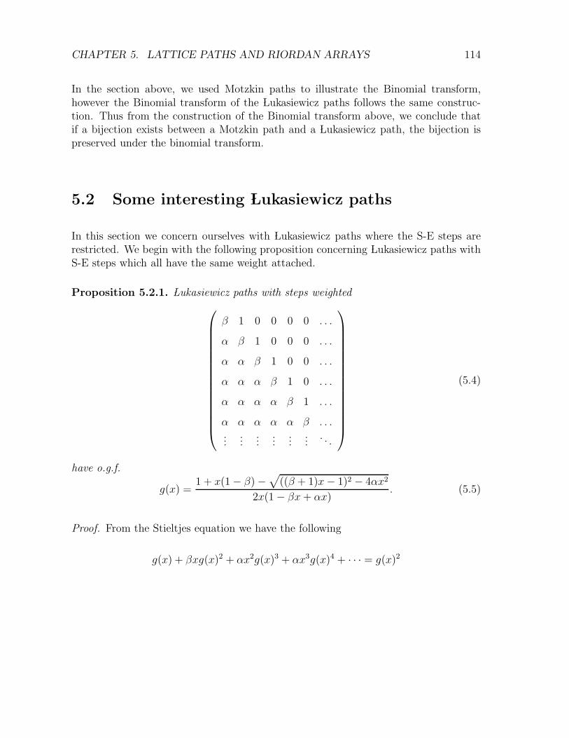
CHAPTER 5. LATTICE PATHS AND RIORDAN ARRAYS 114
In the section above, we used Motzkin paths to illustrate the Binomial transform,however the Binomial transform of the Lukasiewicz paths follows the same construc-tion. Thus from the construction of the Binomial transform above, we conclude thatif a bijection exists between a Motzkin path and a Lukasiewicz path, the bijection ispreserved under the binomial transform.
5.2 Some interesting Lukasiewicz paths
In this section we concern ourselves with Lukasiewicz paths where the S-E steps arerestricted. We begin with the following proposition concerning Lukasiewicz paths withS-E steps which all have the same weight attached.
Proposition 5.2.1. Lukasiewicz paths with steps weighted
β 1 0 0 0 0 . . .
α β 1 0 0 0 . . .
α α β 1 0 0 . . .
α α α β 1 0 . . .
α α α α β 1 . . .
α α α α α β . . ....
......
......
.... . .
(5.4)
have o.g.f.
g(x) =1 + x(1 − β) −
√
((β + 1)x− 1)2 − 4αx2
2x(1 − βx + αx). (5.5)
Proof. From the Stieltjes equation we have the following
g(x) + βxg(x)2 + αx2g(x)3 + αx3g(x)4 + · · · = g(x)2

CHAPTER 5. LATTICE PATHS AND RIORDAN ARRAYS 115
so
g(x) = 1 + βxg(x) + α(xg(x))2(1 + xg(x) + (xg(x))2 + . . . )
= 1 + βxg(x) +α(xg(x))2
1 − xg(x)
and solving for g(x) we have
g(x) =1 + x(1 − β) −
√
((β + 1)x− 1)2 − 4αx2
2x(1 − βx + αx).
Now, we look at two particular Lukasiewicz paths, where the possible S-E steps havethe same weight.
5.2.1 Lukasiewicz paths with no odd south-east steps
Let us look at the Lukasiewicz paths that have no odd south-east steps so we haverelated Stieltjes steps
β0,0 1 0 0 0 0 . . .0 β1,1 1 0 0 0 . . .
α2,0 0 β2,2 1 0 0 . . .0 α3,1 0 α3,3 1 0 . . .
α4,0 0 α4,2 0 β4,4 1 . . .0 α5,1 0 α5,3 0 β5,5 . . ....
......
......
.... . .
, (5.6)
and from the Stieltjes equation we have
βf(x) + α2,0x2(f(x))3 + α4,0x
4(f(x))5 + · · · =f(x) − 1
x.
Rearranging gives
1 + βxf(x) + α2,0x3(f(x))3 + α4,0x
5(f(x))5 + · · · = f(x).

CHAPTER 5. LATTICE PATHS AND RIORDAN ARRAYS 116
Now, let y = xf(x),
1 + βy + αy3 + αy5 + · · · =y
x.
Solving we have
1 + βy + αy3(1 + y2 + . . . ) =y
x
x(1 − y2)(1 + βy) + xαy3 = y(1 − y2)
x + xβy − xy2 − xβy3 + xαy3 = y − y3.
Solving for x we have
x + xβy − xy2 − xβy3 + xαy3 = y − y3
x =y − y3
1 + βy − y2 + y3(α− β).
andy3(xα− xβ + 1) − xy2 + y(xβ − 1) + x = 0.
Solving for y, the first few terms of the g.f. expansion are
x + βx2 + β2x3 + . . .
Example. For the (1, 1)- Lukasiewicz paths of the form above we have the g.f.
x
3−
2√x2 − 3x + 3 sin
( arcsinx(2x2 − 9x− 18)
2(x2 − 3x + 3)3/2
3
)
3
of the sequence 1, 1, 1, 2, 5, . . . (A101785). The paths corresponding to length 4 are illus-
trated below.
x
y
x
y
x
y

CHAPTER 5. LATTICE PATHS AND RIORDAN ARRAYS 117
x
y
x
y
According to [124], (A101785) also counts the number of ordered trees with n edges in
which every non-leaf vertex has an odd number of children. The corresponding Riordan
array is(
1 − x2
1 + x− x2,x(1 − x2)
1 + x− x2
)−1
.
5.2.2 Lukasiewicz paths with no even south-east steps
Let us look at the Lukasiewicz Paths that have no even south-east steps so we haverelated Stieltjes steps
β0,0 1 0 0 0 0 . . .α1,0 β1,1 1 0 0 0 . . .0 α2,1 β2,2 1 0 0 . . .
α3,0 0 α3,2 β3,3 1 0 . . .0 α4,1 0 α4,3 β4,4 1 . . .
α5,0 0 α5,2 0 α5,4 β5,5 . . ....
......
......
.... . .
. (5.7)
and again from the Stieltjes equation we have
βf(x) + α1,0x(f(x))2 + α3,0x3(f(x))4 + · · · =
f(x) − 1
x.
Rearranging we have
1 + βxf(x) + αx2(f(x))2 + α4,0x4(f(x))4 + · · · = f(x).

CHAPTER 5. LATTICE PATHS AND RIORDAN ARRAYS 118
Let y = xf(x), then
1 + βy + αy2 + αy4 + · · · =y
x.
Solving we have
1 + βy + αy2(1 + y2 + . . . ) =y
x
x(1 − y2)(1 + βy) + xαy2 = y(1 − y2)
x + xβy − xy2 − xβy3 + xαy2 = y − y3
and solving for x we have
x =y − y3
1 + βy + y2(α− 1) − βy3
andx + y(xβ − 1) + xy2(α− 1) + y3(1 − xβ) = 0.
Solving for y above we obtain the first few terms of the g.f. expansion as
x + βx2 + x3(α + β2) + βx4(3α + β2) + . . . .
The corresponding Riordan array is(
1 − x2
1 + x− x2,x(1 − x2)
1 + x− x2
)−1
.
Example. The (1, 1)- Lukasiewicz paths of the form above have g.f.
2√
3 sin
( arcsin3√
3x
2|x− 1|3
)
3
of the sequence with first few terms 1, 1, 2, 4, 10, 26, 73, . . .(A049130). We illustrate the
paths of length 4 below.
x
y
x
y
x
y

CHAPTER 5. LATTICE PATHS AND RIORDAN ARRAYS 119
x
y
x
y
x
y
x
y
x
y
x
y
x
y
5.3 A (β, β)- Lukasiewicz path
From (5.5) above, if α = β we have the g.f.
xg(x) =1 + x(1 − β) −
√
((β − 1)x)2 − 2x(β + 1)
2.
Let us look at an interesting example.
Example. The (2, 2)- Lukasiewicz paths have g.f.
xg(x) =1 − x−
√x2 − 6x + 1
2,

CHAPTER 5. LATTICE PATHS AND RIORDAN ARRAYS 120
which is the g.f. of the sequence with first few terms 1, 2, 6, 22, . . . (A006318). The
corresponding paths for n = 3 are shown below.
x
v1v2v3 = 4
y
x
v1v2v3 = 4
y
x
v1v2v3 = 8
y
x
v1v2v3 = 4
y
x
v1v2v3 = 2
y
The above example leads us to the next section where we provide a bijection betweencertain Lukasiewicz paths and Schroder paths.
5.3.1 A bijection between the (2,2)- Lukasiewicz and Schroder
paths
In this section we give a constructive proof of a bijection between the (2,2)- Lukasiewiczpaths and the Schroder paths. Firstly we introduce the different steps possible in the(2,2)- Lukasiewicz paths and the Schroder paths. u is the the N-E step (1, 1), and d theS-E step (1,−1), in both the Lukasiewicz and the Schroder paths. E steps possible areb = (1, 0) in the Lukasiewicz paths and b+ = (2, 0) in the Schroder paths. We denote b1and b2 the two choice of colours for the E steps in the Lukasiewicz paths. Lukasiewiczsteps are denoted ln = (1,−n). We denote d1 and d2 the two choice of colours for the

CHAPTER 5. LATTICE PATHS AND RIORDAN ARRAYS 121
S-E steps in the Lukasiewicz paths, and similarly ln1 and ln2 the choice of Lukasiewiczsteps.
Denote Ln the set of (2, 2)- Lukasiewicz paths of length n and S2n the set of Schroderpaths of length 2n. Now, we construct a map φ : Ln → S2n. Given a (2, 2)- Lukasiewiczpath P of length n we can obtain a lattice path φ(P ) of length 2n by the followingprocedure,
1. u remains unchanged
2. Replace b1 with b+, and b2 with a ud step.
3. Replace d1 with b+d, and d2 with a udd step.
4. Replace ln1 with b+dn, and ln2 with udn+1
Conversely, we can obtain the (2, 2)- Lukasiewicz paths of length n from the Schroderpaths of length 2n by the following procedure,
1. u remains unchanged
2. Replace b+ with b1 and ud with a b2 step.
3. Replace b+d with d1, and udd with a d2 step.
4. Replace b+dn with ln1 , and udn+1 with ln2 .
Let us look at the paths for n = 4

CHAPTER 5. LATTICE PATHS AND RIORDAN ARRAYS 122
b2 b1 b1 udb+b+ b1 b2 b1 b+udb+
b1 b1 b2b+b+ud b2 b2 b1 ududb+
b2 b1 b2udb+ud b1 b2 b2
b+udud
b2 b2 b2ududud b1 b1 b1 b+b+b+
d1 b1 ub+db+d2 b1 uuddb+
d1 b2ub+dud d2 b2
uuddud
b1d1 b+ub+d b1
d2 b+uudd
b2d1 udub+d b2
d2 ududdd
b1 d1 ub+b+db1 d2 ub+udd
b2 d1 uudb+db2 d2 uududd
l1uub+dd
l2uuuddd

CHAPTER 5. LATTICE PATHS AND RIORDAN ARRAYS 123
5.4 A bijection between certain Lukasiewicz and
Motzkin paths
The g.f. of interest here is that of the inverse binomial transform of the Catalannumbers, also known as the Motzkin sums [124]. The tridiagonal Stieltjes matrixcorresponding to the Motzkin sums, which count the Motzkin paths of length n withno horizontal steps at level 0 has the form
0 1 0 0 . . .1 1 1 0 . . .0 1 1 1 . . .0 0 1 1 . . ....
......
. . .
,
the first column of the related Riordan array having g.f. in continued fraction form of
1
1 − x2
1 − x− x2
1 − x− x2
. . .
(A005043).
The Stieltjes matrix corresponding to the Lukasiewicz steps has first few entries
0 1 0 0 . . .1 0 1 0 . . .1 1 0 1 . . .1 1 1 0 . . ....
......
. . .
,
with the first column of the related Riordan array satisfying the equation
(g(x))2(x + x2) − g(x)(1 + x) + 1 = 0.
Solving the equation above gives
g(x) =
√3x− 1
√−x− 1 + x + 1
2x(x + 1),

CHAPTER 5. LATTICE PATHS AND RIORDAN ARRAYS 124
which again counts the sequence of Motzkin paths (A005043).
Here we give a constructive proof of a bijection between the (1,0)- Lukasiewicz pathsand the Motzkin paths, without the possibility of a level steps on the x axis. Again, werecall that u represents N-E step (1, 1), d the S-E step (1,−1). E steps are b = (1, 0)and Lukasiewicz steps are ln = (1,−n),
Denote Mn the set of Motzkin paths of length n with no level steps on the x-axis and Ln
the set of (1, 0)- Lukasiewicz paths of length n. Now, we construct a map φ : Mn → Ln.Given a (1, 1)-Motzkin path P of length n with no level steps on the x-axis, we canobtain a lattice path φ(P ) of length n by the following procedure,
1. We move along the path until we find the first S-E(d) step, we then move to thestep before the S-E step.
• If this is a ud step move onto the next S-E step
• if this is a bd step, it now becomes ul ( . . . ubbbbudbubbduddd · · · → . . . ubbbbudbubuluddd . . .).
2. Now, we move to the next step left of the ul,
• if this is ud step we stop and move onto the next S-E step( . . . ubbbbudbuduluddd · · · →. . . ubbbbudbuuduluddd . . . ).
• If this is a b step bul becomes uul2( . . . ubbbbudbubuluddd · · · → . . . ubbbbudbuuul2uddd . . .).
• If the step is a u, we now have uul giving N-E and a Lukasiewicz step in suc-cession of the same length. Since these are the same length we now proceedto the next S-E step. ( . . . ubbbbudbuuuludddd · · · → . . . ubbbbudbuuuludddd . . .).
3. Repeat 1 and 2 until their are no remaining E steps.
Conversely, we can obtain the (1, 1)-Motzkin paths of length n with no level steps onthe x-axis from the (1, 0)- Lukasiewicz paths of length n by the following procedure,
1. Start at the right most l or d step. If the next step to the left of this is u, stopand move on to the next l or d step.

CHAPTER 5. LATTICE PATHS AND RIORDAN ARRAYS 125
2. If the next step is a d step, starting with the right most u step, we find the cor-responding u step at the level of the d step. We now leave both these unchangedand move to the next left d or l step.
3. If the next step is a step ln, starting with the u step at the corresponding level,we count n+ 1 corresponding u steps, ignoring any ud steps between the u steps.The un+1ln step now becomes ubnd.
4. We move onto the next d or l step and repeat. Repeat until all l steps have beenremoved.
Let us illustrate the moves in two paths below
. . . ubbbudbudbdud · · · → . . . ubbbudbudulud · · · → . . . ubbbuduudul2ud · · · →. . . ubbuuduudul3ud · · · → . . . ubuuuduudul4ud · · · → . . . uuuuuduudul5ud . . .
l
l2l3
l4l5
Conversely we have
uuuuuduudul5ud · · · → . . . ubbbudbudbdud . . .
l5

CHAPTER 5. LATTICE PATHS AND RIORDAN ARRAYS 126
. . . ubbuuubudbdddd · · · ↔ . . . ubbuuubudulddd · · · ↔ . . . ubbuuuuudul2ddd · · · ↔. . . ubbuuuuudul2ddd · · · ↔ . . . ubuuuuuudul2ddl · · · ↔ . . . uuuuuuuudul2ddl2 . . .
l
l2 l2
l2
l2
l2

CHAPTER 5. LATTICE PATHS AND RIORDAN ARRAYS 127
Example. We look at the paths for n = 3
ubbduuul2
udud udud
uudd uudd
We look at the paths for n = 4
Example.
ubbbd
uuuul3
udubduduul
ubdud uulud uubdd uuuld
ubudduuudl
uudbduudul
5.5 Lattice paths and exponential generating func-
tions
In this section we study certain paths that are enumerated by e.g.f.’s. Firstly, weintroduce the following proposition
Proposition 5.5.1. Lukasiewicz paths with level and north east steps of all the same
weight which are enumerated by e.g.f.’s satisfy the ordinary differential equation
d
dxf(x) = f(x)(αex + β − α). (5.8)

CHAPTER 5. LATTICE PATHS AND RIORDAN ARRAYS 128
Proof. We begin by looking at exponential Riordan arrays of the form L = [f(x), x].
Expanding the first column of the matrix equation L = LS where
L =
β0,0 1 0 0 0 0 . . .
α1,0 β1,1 1 0 0 0 . . .
α2,0 α2,1 β2,2 1 0 0 . . .
α3,0 α3,1 α3,2 β3,3 1 0 . . .
α4,0 α4,1 α4,2 α4,3 β4,4 1 . . .
α5,0 α5,1 α5,2 α5,3 α5,4 β5,5 . . ....
......
......
.... . .
, (5.9)
we have
d
dxf(x) = β0,0f(x) + α1,0f(x)x + α2,0f(x)
x2
2!+ α3,0f(x)
x3
3!+ . . .
= f(x)(β0,0 + α1,0x + α2,0x2
2!+ α3,0
x3
3!+ . . . ).
Now let α(x) = β0,0 + α1,0x + α2,0
x2
2!+ α3,0
x3
3!+ · · · =
∑∞n=0 αn,0
xn
n!, α0,0 = β0,0
d
dxf(x) = f(x)α(x).
If α = α1,0 = α2,0 . . . , β0,0 = β, then
d
dxf(x) = f(x)β + f(x)(αx + α
x2
2!+ α
x3
3!+ . . . )
= f(x)β + αf(x)(ex − 1)
= f(x)(αex + β − α).

CHAPTER 5. LATTICE PATHS AND RIORDAN ARRAYS 129
Example. Lukasiewicz paths enumerated by e.g.f.’s with no level step satisfy the ODE
f(x)(−α + αex) =d
dxf(x).
Solving for f(x) we get the e.g.f. of the sequence with first few terms which expand as
1, α, α, (3α2 + α), (10α2 + α), (15α3 + 25α2 + α), . . . (A000296).
Corollary 5.5.2. Lukasiewicz paths with α, β = 1 are enumerated by the e.g.f. of the
Bell numbers
Proof. Solving the differential equation
d
dxf(x) = f(x)(αex + β − α),
results in e.g.f.’s of the form
eαex−α+βx−αx.
For α, β = 1 we have
f(x) = eex−1
which is the e.g.f. of the Bell numbers.
Now, we expand eαex−α+βx−αx to study the Lukasiewicz steps which are enumerated by
the Bell numbers, the first few terms in the series expand as
1 + βx + (α + β2)x2
2!+ (3αβ + α + β3)
x3
3!+ (3α2 + 6αβ2 + 4αβ + α + β4)
x4
4!+
(15α2β + 10α2 + 10αβ3 + 10αβ2 + 5αβ + α + β5)x5
5!+
(15α3 + 45α2β2 + 60α2β + 25α2 + 15αβ4 + 20αβ3 + 15αβ2 + 6αβ + α + β6)x6
6!+ . . .

CHAPTER 5. LATTICE PATHS AND RIORDAN ARRAYS 130
The corresponding Stieltjes matrix related to the Lukasiewicz path expansion of theBell numbers begins
β 1 0 0 0 . . .α β 1 0 0 . . .α 2α β 1 0 . . .α 3α 3α β 1 . . .α 4α 6α 4α β . . ....
......
......
. . .
.
The related Riordan array has the form
[eα(eβx−1)+x(β−α), x].
We note that
n![xn]eα(eβx−1)+x(β−α) =
n∑
k=0
n!
k!
k∑
i=0
1
i!
i∑
j=0
(−1)j(
ij
)
(i− j)kαi(β − α)n−k
(n− k)!.
We see from the above that we now have a Stieljtes matrix of Lukasiewicz steps thatalso enumerates the Bell numbers. We note that we have previously encountered theBell numbers in the form of the continued fraction expansion [56]
1
1 − βx− αx2
1 − 2βx− 2αx2
1 − 3βx− 3αx2
1 − 4βx− 4αx2
. . .
.
The first few terms of this power series expands as
1 + βx + (α + β2)x2 + (4αβ + β3)x3 + (3α2 + 11αβ2 + β4)x4+
(25α2β + 26αβ3 + β5)x5 + (15α3 + 130α2β2 + 57αβ4 + β6)x6+
(210α3β + 546α2β3 + 120αβ5 + β7)x7 . . .

CHAPTER 5. LATTICE PATHS AND RIORDAN ARRAYS 131
The related tridiagonal Stieltjes matrix has first few rows
β 1 0 0 0 . . .α 2β 1 0 0 . . .0 2α 3β 1 0 . . .0 0 3α 4β 1 . . .0 0 0 4α 5β . . .0 0 0 0 5α . . ....
......
.... . .
,
and related Riordan array has the form
[
eα
β2 (eβx−1)+x
(
β2−α
β
)
,eβx − 1
β
]
.
We note that
n![xn]eα
β2 (eβx−1)+x
(
β2−α
β
)
=n∑
k=0
n!
k!
k∑
i=0
1
i!
i∑
j=0
(−1)j(
ij
)
(β(i− j))k( αβ2 )i(
β − αβ
)(n−k)
(n− k)!.
From the above we see that a bijection between the Lukasiewicz and Motzkin pathsthat enumerate the Bell numbers exists.
5.6 Lattice paths and reciprocal sequences
In this section we will look at lattice paths that relate to certain set partitions. Beforewe proceed we take this opportunity to define set partitions and the subsets of setpartitions that will be of interest to us in this chapter. In [56], Flajolet shows abijection between weighted lattice paths and set partitions both counted by the Bellnumbers. We use this bijection to study the subsets of partitions which relate to certainpaths.
Definition 5.6.1. [81] Let X be a set. A set partition of X is a collection P on
nonempty, pairwise disjoint subsets of X whose union is X. Each element of P is called
a block of the partition. The cardinality of P (which may be infinite) is called the number
of blocks of the partition.

CHAPTER 5. LATTICE PATHS AND RIORDAN ARRAYS 132
For example if X = {1, 2, 3, 4, 5, 6, 7, 8}, then P = {1, 6}{3, 4}{2, 5, 7, 8}.
Definition 5.6.2. [81] Let S(n, k) be the number of set partitions of {1, 2, . . . , n} into
exactly k blocks. S(n, k) is called a Stirling number of the second kind. Let B(n) be the
total number of set partitions of {1, 2, . . . , n}. The sequence B(n) is called the sequence
of Bell numbers.
Before we proceed we note that some generating functions which we will encounterin the chapter below, and that we have previously encountered in Chapter 4, countcertain subsets of set partitions, so we take this opportunity to define the partitionsthat will be of interest to us here.
Definition 5.6.3. [80] A partition of [n] = {1, 2, . . . , n} is called connected if no
proper subinterval of [n] is a union of blocks (sometimes referred to as irreducible dia-
grams).
Definition 5.6.4. [80] irreducible partition are partitions which cannot be “factored”
into sub partitions, i.e. partitions of [n] for which 1 and n are in the same connected
component.
connected irreducible
Figure 5.1: A representation of partitions [80]
In the section below we study paths related to g.f.’s of the form
z(x) =1
x
(
1 − 1
g(x)
)
. (5.10)
As this relates closely to the reciprocal sequence of the g.f. g(x), we will refer tothe sequence z(x) as the adjusted reciprocal sequence throughout this chapter. Let usrecall the definition of reciprocal function from [162] which we will use to calculate theadjusted reciprocal sequence.
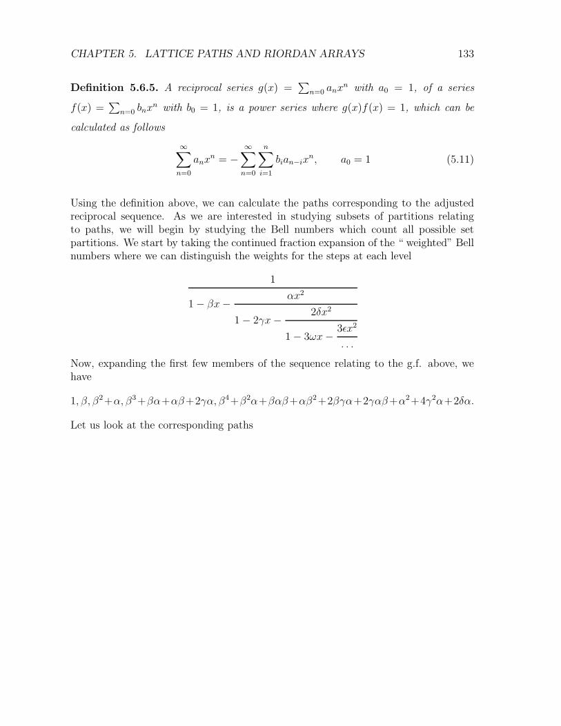
CHAPTER 5. LATTICE PATHS AND RIORDAN ARRAYS 133
Definition 5.6.5. A reciprocal series g(x) =∑
n=0 anxn with a0 = 1, of a series
f(x) =∑
n=0 bnxn with b0 = 1, is a power series where g(x)f(x) = 1, which can be
calculated as follows
∞∑
n=0
anxn = −
∞∑
n=0
n∑
i=1
bian−ixn, a0 = 1 (5.11)
Using the definition above, we can calculate the paths corresponding to the adjustedreciprocal sequence. As we are interested in studying subsets of partitions relatingto paths, we will begin by studying the Bell numbers which count all possible setpartitions. We start by taking the continued fraction expansion of the “ weighted” Bellnumbers where we can distinguish the weights for the steps at each level
1
1 − βx− αx2
1 − 2γx− 2δx2
1 − 3ωx− 3ǫx2
. . .
Now, expanding the first few members of the sequence relating to the g.f. above, wehave
1, β, β2+α, β3+βα+αβ+2γα, β4+β2α+βαβ+αβ2+2βγα+2γαβ+α2+4γ2α+2δα.
Let us look at the corresponding paths

CHAPTER 5. LATTICE PATHS AND RIORDAN ARRAYS 134
β
α + β2
β3 + 2γα + αβ + βα
β4 + β2α + βαβ + αβ2 + 2βγα + 2γαβ + α2 + 4γ2α + 2δα
We note that the reciprocal sequence is calculated recursively, so we now proceedby using the paths above to calculate the paths of the adjusted reciprocal sequencerecursively. Let us expand the first few paths of this recursive procedure. Firstlyexpanding (5.11) for the first few elements we have
• a1x = −(b1a0)x,
– a1 consists of the paths of b1.
• a2x2 = −(b1a1 + b2a0)x
2,
– a2 consists of the paths of b2 which can not be formed from the union ofpaths b1a1 = b21.
• a3x3 = −(b1a2 + b2a1 + b3a0)x
3,
– a3 consists of the paths of b3 which can not be formed from the union ofpaths of b1a2 = b1(b2 − b21) and b2a1 = b2b1.
• a4x4 = −(b1a3 + b2a2 + b3a1 + b4a0)x
4,
– a4 consists of the paths of b4 which can not be formed from the union ofpaths of b1a3 = b1(b3 − b1(b2 − b21)), b2a2 = b2(b2 − b21),b3b1.
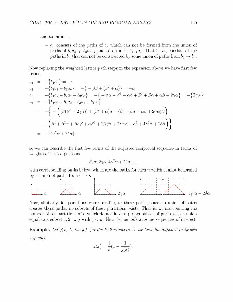
CHAPTER 5. LATTICE PATHS AND RIORDAN ARRAYS 135
and so on until
– an consists of the paths of bn which can not be formed from the union ofpaths of b1an−1, b2an−2 and so on until bn−1a1. That is, an consists of thepaths in bn that can not be constructed by some union of paths from b0 → bn.
Now replacing the weighted lattice path steps in the expansion above we have first fewterms
a1 = −{
b1a0}
= −β
a2 = −{
b1a1 + b2a0}
= −{
− ββ + (β2 + α)}
= −α
a3 = −{
b1a2 + b2a1 + b3a0}
= −{
− βα− β3 − αβ + β3 + βα + αβ + 2γα}
= −{
2γα}
a4 = −{
b1a3 + b2a2 + b3a1 + b4a0}
= −{
−(
(β(β3 + 2γα)) + (β2 + α)α + (β3 + βα + αβ + 2γα)β
)
+
(
β4 + β2α + βαβ + αβ2 + 2βγα + 2γαβ + α2 + 4γ2α + 2δα
)}
= −{4γ2α + 2δα}
so we can describe the first few terms of the adjusted reciprocal sequence in terms ofweights of lattice paths as
β, α, 2γα, 4γ2α + 2δα . . .
with corresponding paths below, which are the paths for each n which cannot be formedby a union of paths from 0 → n
β α 2γα 4γ2α + 2δα
Now, similarly, for partitions corresponding to these paths, since no union of pathscreates these paths, no subsets of these partitions exists. That is, we are counting thenumber of set partitions of n which do not have a proper subset of parts with a unionequal to a subset 1, 2, ..., j with j < n. Now, let us look at some sequences of interest.
Example. Let g(x) be the g.f. for the Bell numbers, so we have the adjusted reciprocal
sequence
z(x) =1
x(1 − 1
g(x)),

CHAPTER 5. LATTICE PATHS AND RIORDAN ARRAYS 136
with first few elements 1, 1, 2, 6, 22, 92, 426, 2146, . . .(A074664). This sequence counts
the number of set partitions of n which do not have a proper subset of parts with a
union equal to a subset 1, 2, ..., j with j < n. Fig. (5.2) shows the first few paths and
corresponding partitions
Example. We consider the Young Tableaux numbers, which count all the partitions
for each n which have less than two element in each partition. The g.f. of the Young
Tableaux numbers has a continued fraction expansion of the form
1
1 − x−x2
1 − x−2x2
1 − x−3x2
1 − x− 4x2. . .
.
We look at the adjusted reciprocal sequence for the Young Tableaux. The first few coef-
ficients of z(x) expand as 1, 1, 1, 3, 7, 23, 71, 255, . . .(A140456), so this sequence counts
the number of set partitions of n, considering only sets of partitions of size less than or
equal to two, which do not have a proper subset of parts with a union equal to a subset
1, 2, ..., j with j < n. Fig. (5.3) shows the first few paths and corresponding partitions.
Example. We consider the Bessel numbers, which count the number of non-overlapping
partitions. The Bessel numbers have a continued fraction expansion of the form
1
1 − x−x2
1 − 2x−x2
1 − 3x−x2
1 − 4x− x2. . .
.

CHAPTER 5. LATTICE PATHS AND RIORDAN ARRAYS 137
{1} {1 2}
{1 3}{2} , {1 2 3}
{1 4}{2}{3},{1 2 3 4},
{1 2 4}{3},{1 3 4}{2}{1 3}{2 4},
{1 4}{2 3}
{ 1 5}{2}{3}{4},
{ 1 3 5}{2}{4},
{ 1 2 5}{3}{4},{ 1 2 3
5}{4},
{ 1 4 5}{2}{3},{1 2 3 4 5},
{ 1 3 4 5}{2},{ 1 2 4 5}{3}.
{1 5}{2 4}{3},
{1 4}{2 3 5},
{1 5}{2 3 4},
{1 3 5}{2 4}{1 4}{2 5}{3},
{1 3 4}{2 5}{1 3}{2 5}{4},
{1 5}{2 3}{4}{1 3}{ 2 4 5},
{ 1 4 5}{2 3}
{1 4}{2}{3 5} ,
{1 5}{2}{3 4}{3 4}{1 2 5},
{3 5}{1 2 4}
Figure 5.2: Paths and partitions corresponding to the adjusted reciprocal sequence of
the Bell numbers
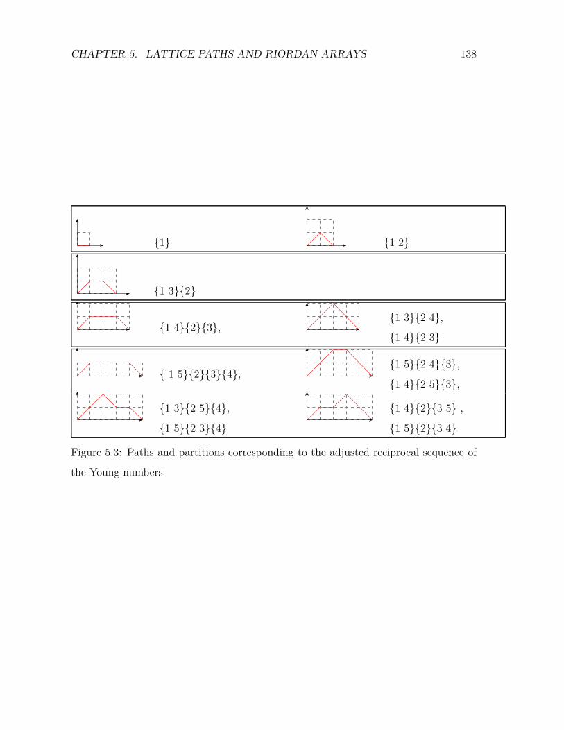
CHAPTER 5. LATTICE PATHS AND RIORDAN ARRAYS 138
{1} {1 2}
{1 3}{2}
{1 4}{2}{3},{1 3}{2 4},
{1 4}{2 3}
{ 1 5}{2}{3}{4},{1 5}{2 4}{3},
{1 4}{2 5}{3},
{1 3}{2 5}{4},
{1 5}{2 3}{4}{1 4}{2}{3 5} ,
{1 5}{2}{3 4}
Figure 5.3: Paths and partitions corresponding to the adjusted reciprocal sequence of
the Young numbers

CHAPTER 5. LATTICE PATHS AND RIORDAN ARRAYS 139
{1} {1 2}
{1 3}{2} , {1 2 3}
{1 4}{2}{3},
{1 2 4}{3},
{1 3 4}{2},{1 2 3 4}{1 4}{2 3}
{ 1 5}{2}{3}{4},
{ 1 3 5}{2}{4},
{ 1 2 5}{3}{4},{ 1 2 3
5}{4},
{ 1 4 5}{2}{3},{1 2 3 4 5},
{ 1 3 4 5}{2},{ 1 2 4 5}{3}.
{1 5}{2 4}{3},
{1 5}{2 3 4},
{1 3 5}{2 4}
{1 5}{2 3}{4}{ 1 4 5}{2 3}
{1 5}{2}{3 4}{3 4}{1 2 5},
Figure 5.4: Paths and partitions corresponding to the adjusted reciprocal sequence of
the Bessel numbers
Then the adjusted reciprocal sequence z(x) for the Bessel numbers has first few co-
efficients of z(x) given by 1, 1, 2, 5, 15, 51, 189, 748, 3128, 13731 . . .(A153197), so this
sequence counts the number of set partitions of n, only considering sets of non - over-
lapping partitions, which do not have a proper subset of parts with a union equal to
a subset 1, 2, ..., j with j < n. Fig. (5.4) shows the first few paths and corresponding
partitions.
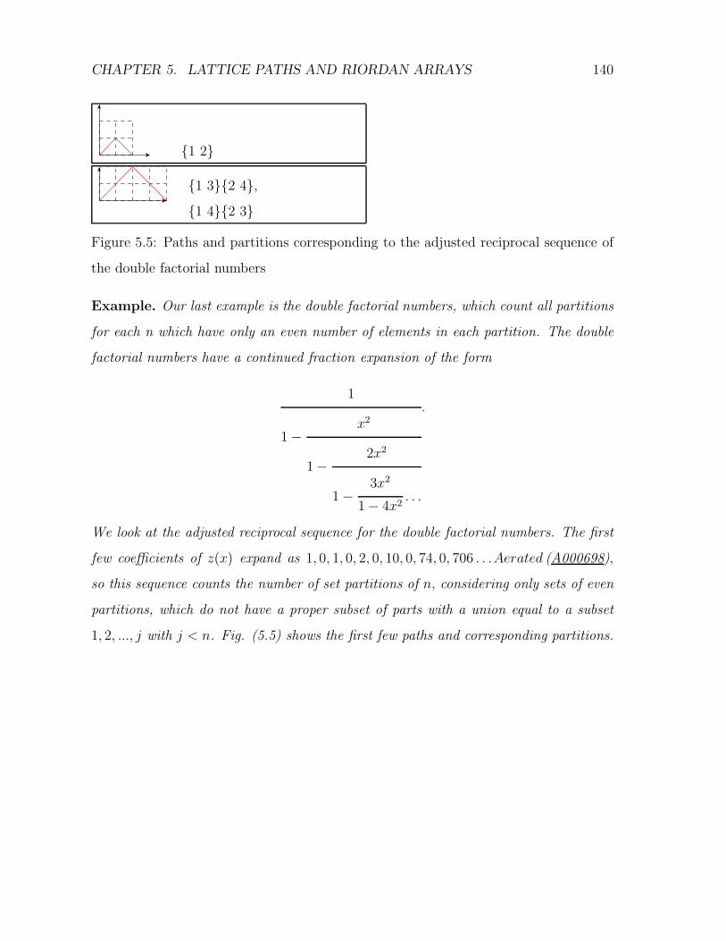
CHAPTER 5. LATTICE PATHS AND RIORDAN ARRAYS 140
{1 2}
{1 3}{2 4},
{1 4}{2 3}
Figure 5.5: Paths and partitions corresponding to the adjusted reciprocal sequence of
the double factorial numbers
Example. Our last example is the double factorial numbers, which count all partitions
for each n which have only an even number of elements in each partition. The double
factorial numbers have a continued fraction expansion of the form
1
1 −x2
1 −2x2
1 −3x2
1 − 4x2. . .
.
We look at the adjusted reciprocal sequence for the double factorial numbers. The first
few coefficients of z(x) expand as 1, 0, 1, 0, 2, 0, 10, 0, 74, 0, 706 . . .Aerated (A000698),
so this sequence counts the number of set partitions of n, considering only sets of even
partitions, which do not have a proper subset of parts with a union equal to a subset
1, 2, ..., j with j < n. Fig. (5.5) shows the first few paths and corresponding partitions.

CHAPTER 5. LATTICE PATHS AND RIORDAN ARRAYS 141
5.7 Bijections between Motzkin paths and constrained
Lukasiewicz paths
In section 5.6 we have looked at the adjusted reciprocal sequence relating to Motzkinpaths. Let us now look at the adjusted reciprocal sequence for the Lukasiewicz paths.From section 5.2 we have the following continued fraction expansion for Lukasiewiczpaths with all Lukasiewicz steps of weight α and level steps of weight β,
1
1 + x(1 − β) +x(x(β − α) − 1)
1 + x(1 − β) +x(x(β − α) − 1)
. . .
Similarly, as for the Motzkin paths shown in section 5.6, the adjusted reciprocal sequencecounts the Lukasiewicz paths that do not return to the x axis. Looking at one suchexample of these paths, with β = 0 and α = 1 we have the
g(x) =1
1 + x(1) +x(x(−1) − 1)
1 + x(1) +x(x(−1) − 1)
. . .
so the adjusted reciprocal sequence
z(x) =1
x(1 − 1
g(x))
is the sequence of Motzkin numbers (A001006).
From above, we introduce the following bijection between the (1, 1)-Motzkin paths oflength n and the (1, 0)- Lukasiewicz paths of length n + 2 which do not return to thex-axis until the final step.
Before we give the bijection, let us look at the paths corresponding to n = 1, 2, 3 and4. For n = 1 we have the following path
buul

CHAPTER 5. LATTICE PATHS AND RIORDAN ARRAYS 142
For n = 2 we have the following two paths
bb
uuul2
ud uudd
For n = 3 we have the following four paths
bbb
uuul2
udbuudl
ubduuld
buduudul
For n = 4 we have the following nine paths
ubbd uuuul2d bubduuuull
ubdbuuulul
uudd uuuddd
udud uududd bbuduuuudl2
udbb
uuduul2
budb
uuudul2
bbbb
uuuuul4
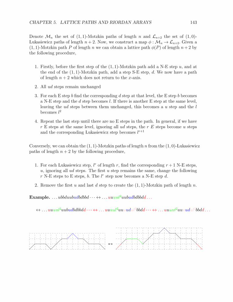
CHAPTER 5. LATTICE PATHS AND RIORDAN ARRAYS 143
Denote Mn the set of (1, 1)-Motzkin paths of length n and Ln+2 the set of (1, 0)- Lukasiewicz paths of length n + 2. Now, we construct a map φ : Mn → Ln+2. Given a(1, 1)-Motzkin path P of length n we can obtain a lattice path φ(P ) of length n+ 2 bythe following procedure,
1. Firstly, before the first step of the (1, 1)-Motzkin path add a N-E step u, and atthe end of the (1, 1)-Motzkin path, add a step S-E step, d. We now have a pathof length n + 2 which does not return to the x-axis.
2. All ud steps remain unchanged
3. For each E step b find the corresponding d step at that level, the E step b becomesa N-E step and the d step becomes l. If there is another E step at the same level,leaving the ud steps between them unchanged, this becomes a u step and the lbecomes l2
4. Repeat the last step until there are no E steps in the path. In general, if we haver E steps at the same level, ignoring all ud steps, the r E steps become u stepsand the corresponding Lukasiewicz step becomes lr+1
Conversely, we can obtain the (1, 1)-Motzkin paths of length n from the (1, 0)- Lukasiewiczpaths of length n + 2 by the following procedure,
1. For each Lukasiewicz step, lr of length r, find the corresponding r + 1 N-E steps,u, ignoring all ud steps. The first u step remains the same, change the followingr N-E steps to E steps, b. The lr step now becomes a N-E step d.
2. Remove the first u and last d step to create the (1, 1)-Motzkin path of length n.
Example. . . . ubbduubudbdbbd · · · ↔ . . . uuuul2uubudbdbbdd . . .
↔ . . . uuuul2uubudbdbbdd · · · ↔ . . . uuuul2uuuudul2bbdd · · · ↔ . . . uuuul2uuuudul2bbdd . . .
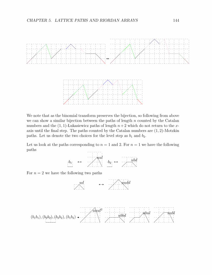
CHAPTER 5. LATTICE PATHS AND RIORDAN ARRAYS 144
We note that as the binomial transform preserves the bijection, so following from abovewe can show a similar bijection between the paths of length n counted by the Catalannumbers and the (1, 1)- Lukasiewicz paths of length n+ 2 which do not return to the x-axis until the final step. The paths counted by the Catalan numbers are (1, 2)-Motzkinpaths. Let us denote the two choices for the level step as b1 and b2.
Let us look at the paths corresponding to n = 1 and 2. For n = 1 we have the followingpaths
b1uul
b2ubd
For n = 2 we have the following two paths
ud uudd
(b1b1), (b2b2), (b2b2), (b1b2)
uuul2
ubbdubul uubl

CHAPTER 5. LATTICE PATHS AND RIORDAN ARRAYS 145
To show the bijection between the (1, 2)-Motzkin paths and the (1, 1)- Lukasiewiczpaths, we have the following procedure:
Denote Cn the set of (1, 2)-Motzkin paths of length n, where the level steps have twochoices namely, b1 and b2, and Wn+2 the set of Lukasiewicz paths of length n+2, whichdo not return to the x-axis until the last step. Now, we construct a map φ : Cn → Wn+2.Given a path P of length n we can obtain a lattice path φ(P ) of length n + 2 by thefollowing procedure,
1. Firstly, before the first step of the (1, 2)-Motzkin path add a N-E step u, and atthe end of the (1, 2)-Motzkin path, add a step S-E step, d. We now have a pathof length n + 2 which does not return to the x axis.
2. All ud steps remain unchanged
3. For each E step b1 find the corresponding d step at that level, the E step b1becomes a N-E step and the d step becomes l. If there is another E step at thesame level, leaving the ud steps between them unchanged, this becomes a u stepand the l becomes l2. E steps b2 remain unchanged
4. Repeat the last step until there are no E steps b1 remaining in the path.
Conversely, we can obtain the (1, 2)-Motzkin paths of length n from the (1, 1)- Lukasiewiczpaths of length n + 2 by the following procedure,
1. For each Lukasiewicz step, lr of length r, find the corresponding r + 1 N-E stepsu, ignoring all ud steps. The first u step remains the same, change the followingr N-E steps to E steps, b. The lr step now becomes a N-E step d.
2. b2 steps remain unchanged, as do ud steps.
3. Remove the first u and last d step to create the (1, 2)-Motzkin paths of length n.
Example.
gives the eight paths

CHAPTER 5. LATTICE PATHS AND RIORDAN ARRAYS 146
. . . ub1b1duub1uddd · · · ↔ . . . uuuul2uuuudldd . . .
. . . ub1b1duub2uddd · · · ↔ . . . uuuul2uubudddd . . .
. . . ub1b2duub1uddd · · · ↔ . . . uuubluuuudldd . . .
. . . ub2b1duub1uddd · · · ↔ . . . uubuluuuudldd . . .
. . . ub2b2duub1uddd · · · ↔ . . . uubbduuuudldd . . .
. . . ub2b1duub2uddd · · · ↔ . . . uubuluubudddd . . .
. . . ub1b2duub2uddd · · · ↔ . . . uuubluubudddd . . .

CHAPTER 5. LATTICE PATHS AND RIORDAN ARRAYS 147
. . . ub2b2duub2uddd · · · ↔ . . . uubbduubudddd . . .

Chapter 6
Hankel decompositions using
Riordan arrays
This chapter is inspired by Peart and Woan [103], who studied Hankel matrices usinga Riordan array decomposition, where the Riordan array has an associated tridiagonalStieltjes matrices. As we saw in the last chapter, these Riordan arrays relate to Motzkinpaths. In this chapter, we study these Hankel matrices, decomposing them in analternative manner, where the related Riordan array in the decomposition has a non-tridiagonal Stieltjes matrix. The Stieltjes matrices are those that relate to Lukasiewiczpaths. In the previous chapter we studied Lukasiewicz paths. In eq. (5.5) fromproposition 5.2.1 we showed that Lukasiewicz paths with steps weighted
β 1 0 0 0 0 . . .α β 1 0 0 0 . . .α α β 1 0 0 . . .α α α β 1 0 . . .α α α α β 1 . . .α α α α α β . . ....
......
......
.... . .
(6.1)
have o.g.f.
xg(x) =1 + x(1 − β) −
√
((β + 1)x− 1)2 − 4αx2
2(1 − βx + αx).
148

CHAPTER 6. HANKEL DECOMPOSITIONS USING RIORDAN ARRAYS 149
In this chapter we look at Hankel matrix decompositions involving Riordan arrayswith generating functions of this form. From studying this alternative decompositionwe study the relationship between Motzkin and Lukasiewicz paths through the mediumof Riordan arrays.
In the first section we will introduce and develop on results relating to Riordan arraysof g.f.’s of the form in [103]. We then introduce results relating to Hankel matricesdecompomposed into Riordan arrays relating to certain Lukasiewicz paths. As theHankel transform is invariant under the Binomial transform, we concern ourselves withg.f.’s of the Binomial transform of certain functions. Finally, before we leave thischapter we look at a second decomposition of a Hankel matrix. Generating functionsrelating to Hankel matrices in this section are unrelated to paths, and are simplyinspired by earlier work in the chapter.
6.1 Hankel decompositions with associated tridiag-
onal Stieltjes matrices
Firstly, let us recall some relevant results relating to Hankel matrices of the form studiedin [103].
Theorem 6.1.1. [103, Theorem 1] Let H = (ank)n,k≥0 be the Hankel matrix generated
by the sequence 1, a1, a2, a3, . . . Assume that H = LDU where
L = (lnk)n,k≥0 =
1 0 0 0 . . .
l1,0 1 0 0 . . .
l2,0 l2,1 1 0 . . .
l3,0 l3,1 l3,2 1 . . .
l4,0 l4,1 l4,2 l4,3 . . ....
......
.... . .
,

CHAPTER 6. HANKEL DECOMPOSITIONS USING RIORDAN ARRAYS 150
D =
d0 0 0 0 . . .
0 d1 0 0 . . .
0 0 d2 0 . . .
0 0 0 d3 . . ....
......
......
, di 6= 0, U = LT .
Then the Stieltjes matrix SL is tridiagonal, with the form
β0 1 0 0 0 0 0
α1 β1 1 0 0 0 0
0 α2 β1 1 0 0 0
0 0 α2 β1 1 0 0
0 0 0 α2 β1 1 0
0 0 0 0 α2 β1 1...
......
......
.... . .
,
where
β0 = a1, α1 = d1, βk = lk+1,k − lk,k+1, αk =dk+1
dk, k ≥ 1.
Following from this result, theorems 2.4.4 and 2.4.5 which we introduced in section 2.4define the Riordan arrays that satisfy theorem 6.1.1. Here, for o.g.f.’s, drawing fromthe continued fraction expansion of the related g.f.’s we offer the following proof,
Proposition 6.1.2. If the Stieltjes matrix S has the form
S =
β0 1 0 0 0 . . .
α1 β1 1 0 0 . . .
0 α2 β1 1 0 . . .
0 0 α2 β1 1 . . ....
......
......
. . .

CHAPTER 6. HANKEL DECOMPOSITIONS USING RIORDAN ARRAYS 151
then the related Riordan array (g(x), xf(x)) has the form(
1
1 − β0x− α1x(xf(x)),
x
1 − β1x− α2x(xf(x))
)
(6.2)
where
xf(x) =−(β1x− 1) −
√
(β1x− 1)2 − 4α2x2
2α2x. (6.3)
Proof. Let g(x) =∑∞
n=0 anxn, with a0 = 1. A continued fraction expansion relating to
the Stieltjes matrix S above has the form [76]
g(x) =1
1 − β0x−α1x
2
1 − β1x−α2x
2
1 − β1x− α2x2
...
=1
1 − β0x− α1x(xf(x)),
where xf(x) is
xf(x) =x
1 − β1x−α2x
2
1 − β1x−α2x
2
1 − β1x− α2x2
...
=1
1 − β1x− α2x(xf(x)).
Solving for xf(x) gives
xf(x) =−(β1x− 1) −
√
(β1x− 1)2 − 4α1x2
2α1x
resulting in eq. (6.3).
Note that if β1 = β0 and α1 = α2 we obtain the Riordan array
(g(x), xg(x)) =
(
1
1 − β0x− α1x(xg(x)),
x
1 − β0x− α1x(xg(x))
)
.

CHAPTER 6. HANKEL DECOMPOSITIONS USING RIORDAN ARRAYS 152
From [76], the Hankel determinant hn of order n of an = [xn]g(x) is
hn = an0αn−11 αn−2
2 . . . α2n−1αn−1.
From the form of the continued fraction expansion of g.f.’s satisfying theorem 6.1.1,the Hankel determinant hn of order n of an = [xn]g(x), when the Riordan array Lsatisfying theorem 6.1.1 has the form (g(x), xf(x)), with a0 = 1, is
hn = an0αn−11 αn−2
2 . . . α22αn−1 = αn−1
1 α∑n−2
i=ii
2 = αn−11 α
n2−3n+22
2 ,
and when the Riordan array L satisfying theorem 6.1.1 has the form (g(x), xg(x)), theHankel determinant is,
hn = an0αn−11 αn−2
2 . . . α22αn−1 = α
∑n−1i=i i
1 = αn2−n
2 .
In this chapter we concern ourselves with the Binomial transform of certain functions.We take this opportunity to present the following result.
Proposition 6.1.3. Let LDLT = H, with H a Hankel matrix, D a diagonal matrix
and L be a Riordan matrix (g(x),f(x))([(g(x),f(x)]) with related Stieltjes matrix S, so
that L−1L = S. Then, the Riordan array related to the binomial transform of the Hankel
matrix H has Stieltjes matrix S + I.
Proof. The Binomial transform of H in matrix form is QHQT where
Q =
1 0 0 0 0 . . .
1 1 0 0 0 . . .
1 2 1 0 0 . . .
1 3 3 1 0 . . ....
......
.... . .
=
(
1
1 − x,
1
1 − x
)
= [ex, x].
Now if LLT = H we have the binomial transform of H
QHQT = QLLTQT
= QL(QL)T

CHAPTER 6. HANKEL DECOMPOSITIONS USING RIORDAN ARRAYS 153
The Stieltjes matrix S of the Riordan array L satisfies the equation L−1L = S. Thus
we wish to show that the Riordan array QL satisfies the equation
(QL)−1QL = L−1Q−1QL = I + S. (6.4)
Firstly we show that
Q−1QL = L + L.
For o.g.f.’s we have
(
1
1 + x,
x
1 + x
)(
1
1 − x,
x
1 − x
)
(g(x), f(x)) =
(
1
1 + x,
x
1 + x
)(
1
1 − xg(
x
1 − x), f(
x
1 − x)
)
.
The first column of the “beheaded” Riordan array above is
11−x
g(
x1−x
)
− 1
x
and the nth column1
1−xg(
x1−x
)
f(
x1−x
)n
x.
Now, left multiplication of the matrix Q−1 gives the resulting first column
1
1 + x
11− x
1+x
g(x) − 1
x1+x
=g(x) − 1
x+ g(x)
and nth column
1
1 + x
11− x
1+x
g(x)f(x)n
x1+x
=g(x)f(x)n
x+ g(x)f(x)n.
These columns form the matrix L + L. Similarly, for e.g.f.’s we have
[e−x, x]d
dx[exg(x), f(x)].

CHAPTER 6. HANKEL DECOMPOSITIONS USING RIORDAN ARRAYS 154
Expanding the first column gives
[e−x, x]d
dx(exg(x)) = [e−x, x](ex
d
dxg(x) + exg(x)) =
d
dxg(x) + g(x),
and for the nth column we have
[e−x, x]
(
exd
dx
(
g(x)f(x)n
n!
)
+ exg(x)f(x)n
n!
)
=d
dx
(
g(x)f(x)n
n!
)
+ g(x)f(x)n
n!.
These columns form the matrix L + L.
Now we have shown for both e.g.f.’s and o.g.f.’s that
Q−1QL = L + L.
Pre-multiplying by the matrix L−1 gives eq. (6.4).
Corollary 6.1.4.
L−1(QnL)−1QnL = nI + S.
Similarly to above, we can show that
(QnL)−1QnL = nL + L,
with the binomial Riordan array
Qn =
(
1
1 − nx,
1
1 − nx
)
for o.g.f.’s and [enx, x] for e.g.f.’s.
The Hankel matrices formed from the series f(x) listed in the table below decomposeaccording to Theorem 6.1.1. That is, H = LDL. For the power series in the tablebelow, D is the diagonal matrix and L is the Riordan array (f(x), xf(x)).

CHAPTER 6. HANKEL DECOMPOSITIONS USING RIORDAN ARRAYS 155
Power series A-number
∑∞n=0
∑⌊n2⌋
k=01
k+1
(
2kk
)(
n2k
)
0n−2kxn1 −
√1 − 4x2
2x2
Aerated (A126120)
∑∞n=0
∑⌊n2⌋
k=01
k+1
(
2kk
)(
n2k
)
xn(1 − x) −
√
(1 − x)2 − 4x2
2x2
(A001006)
∑∞n=0
∑⌊n2⌋
k=01
k+1
(
2kk
)(
n2k
)
2n−2kxn(1 − 2x) −
√
(1 − 2x)2 − 4x2
2x2
(A000108)
∑∞n=0
∑⌊n2⌋
k=01
k+1
(
2kk
)(
n2k
)
3n−2kxn(1 − 3x) −
√
(1 − 3x)2 − 4x2
2x2
(A000108)
......
∑∞n=0
∑⌊n2⌋
k=01
k+1
(
2kk
)(
n2k
)
hn−2kxn(1 − hx) −
√
(1 − hx)2 − 4x2
2x2
In table above, when h = 0 we have the sequence
∞∑
n=0
⌊n2⌋
∑
k=0
1
k + 1
(
2k
k
)(
n
2k
)
0n−2kxn,
which has a non zero term when n = 2k. Thus we have∞∑
n=0
1
n/2 + 1
(
n
n/2
)
xn =∞∑
n=0
1
n + 1
(
2n
n
)
x2n,
the sequence of aerated Catalan numbers. We now offer the following proof by induc-tion.

CHAPTER 6. HANKEL DECOMPOSITIONS USING RIORDAN ARRAYS 156
Proposition 6.1.5. The binomial transform of the sequence
∞∑
n=0
⌊n2⌋
∑
k=0
1
k + 1
(
2k
k
)(
n
2k
)
hn−2kxn
is the sequence∞∑
n=0
⌊n2⌋
∑
k=0
1
k + 1
(
2k
k
)(
n
2k
)
(h + 1)n−2kxn
Proof. We assume true for n and by induction we prove true for n+ 1, that is we prove
the following,
n∑
r=0
(
n
r
) ⌊n2⌋
∑
k=0
1
k + 1
(
2k
k
)(
r
2k
)
hr−2k =
⌊n2⌋
∑
k=0
1
k + 1
(
2k
k
)(
n
2k
)
(h + 1)n−2k
=
⌊n2⌋
∑
k=0
1
k + 1
(
2k
k
)(
n
2k
) n−2k∑
m=0
(
n− 2k
m
)
hm.
Firstly, when n = 0,
0∑
r=0
(
0
r
) ⌊ 02⌋
∑
k=0
1
k + 1
(
2k
k
)(
r
2k
)
hr−2k =
⌊ 02⌋
∑
k=0
1
k + 1
(
2k
k
)(
0
2k
) 0−2k∑
m=0
(
0 − 2k
m
)
hm = 1.
By a change of variable
n∑
r=0
(
n
r
) ⌊n2⌋
∑
k=0
1
k + 1
(
2k
k
)(
r
2k
)
hr−2k =
⌊n2⌋
∑
k=0
1
k + 1
(
2k
k
) n−2k∑
m=0
(
n
2k + m
)(
2k + m
2k
)
hm.

CHAPTER 6. HANKEL DECOMPOSITIONS USING RIORDAN ARRAYS 157
By the cross product of Binomial coefficients we have
⌊n2⌋
∑
k=0
1
k + 1
(
2k
k
) n−2k∑
m=0
(
n
2k + m
)(
2k + m
2k
)
hm =
⌊n2⌋
∑
k=0
1
k + 1
(
2k
k
) n−2k∑
m=0
(
n
2k
)(
n− 2k
m
)
hm
=
⌊n2⌋
∑
k=0
1
k + 1
(
2k
k
)(
n
2k
) n−2k∑
m=0
(
n− 2k
m
)
hm
=
⌊n2⌋
∑
k=0
1
k + 1
(
2k
k
)(
n
2k
)
(h + 1)n−2k.
Riordan arrays formed from the power series f(x) in the table below, once again sat-isfy the decomposition LDLT = H. For the power series in the table below, D is thediagonal matrix where the nth element of D, Dn,n is mn, for some m > 0 and L is theRiordan array (f(x), xf(x)).

CHAPTER 6. HANKEL DECOMPOSITIONS USING RIORDAN ARRAYS 158
Power series A-number
∑∞n=0
∑⌊n2⌋
k=01
k+1
(
2kk
)(
n2k
)
0n−2k2kxn1 −
√1 − 8x2
4x2
Aerated (A052701)
∑∞n=0
∑⌊n2⌋
k=01
k+1
(
2kk
)(
n2k
)
1n−2k2kxn(1 − x) −
√
(1 − x)2 − 8x2
4x2
(A025235)
∑∞n=0
∑⌊n2⌋
k=01
k+1
(
2kk
)(
n2k
)
2n−2k2kxn(1 − 2x) −
√
(1 − 2x)2 − 8x2
4x2
(A071356)
∑∞n=0
∑⌊n2⌋
k=01
k+1
(
2kk
)(
nn−2k
)
3n−2k2kxn(1 − 3x) −
√
(1 − 3x)2 − 8x2
4x2
(A001002)
∑∞n=0
∑⌊n2⌋
k=01
k+1
(
2kk
)(
nn−2k
)
0n−2k3kxn1 −
√1 − 12x2
6x2
Aerated (A005159)
∑∞n=0
∑⌊n2⌋
k=01
k+1
(
2kk
)(
nn−2k
)
3kxn(1 − x) −
√
(1 − x)2 − 12x2
6x2
(A025237)
∑∞n=0
∑⌊n2⌋
k=01
k+1
(
2kk
)(
nn−2k
)
2n−2k3kxn(1 − 2x) −
√
(1 − 2x)2 − 12x2
6x2
(A122871)
∑∞n=0
∑⌊n2⌋
k=01
k+1
(
2kk
)(
nn−2k
)
3n−2k3kxn(1 − 3x) −
√
(1 − 3x)2 − 12x2
6x2
(A107264)...
...
∑∞n=0
∑⌊n2⌋
k=01
k+1
(
2kk
)(
nn−2k
)
hn−2kmkxn(1 − hx) −
√
(1 − hx)2 − 4mx2
2mx2

CHAPTER 6. HANKEL DECOMPOSITIONS USING RIORDAN ARRAYS 159
6.2 Hankel matrices and non-tridiagonal Stieltjes
matrices
Now, as shown in the last section, we looked at Hankel matrices which decomposed intoL1DL1
T , where the Riordan array L1 has an associated tridiagonal Stieltjes matrix.Here, we decompose the Hankel matrix Hf (x), where L = (f(x), xf(x)), into
LB · D · (LB)T (6.5)
where the Riordan array, L1 from the previous section has been decomposed furtherinto the product of two Riordan arrays, the second array being defined throughout thissection as the matrix B, which is the “shifted” Binomial matrix with the first column0n. The first few rows have the form
B =
1 0 0 0 0 . . .0 1 0 0 0 . . .0 1 1 0 0 . . .0 1 2 1 0 . . .0 1 3 3 1 . . ....
......
......
. . .
=
(
1,x
1 − x
)
. (6.6)
The generating function of the first column of the Riordan array L, f(x), is the gen-erating function in eq. (5.5) with α = β = β0. That is, f(x) is the g.f. for Lukasiewiczpaths with east(E) and south-easterly(S-E) steps of the same weight, thus the relatedStieltjes matrix has the form
β0 1 0 0 0 0 . . .β0 β0 1 0 0 0 . . .β0 β0 β0 1 0 0 . . .β0 β0 β0 β0 1 0 . . .β0 β0 β0 β0 β0 1 . . .β0 β0 β0 β0 β0 β0 . . ....
......
......
.... . .
. (6.7)
Thus Hf is the Hankel matrix where an = [xn]f(x), to which we associate the g.f.f(x) =
∑∞n=0 anx
n where
f(x) =1
(1 − (β0 − 1)x) − xf(x)
=1 − (β0 − 1)x−
√
(1 − (β0 − 1)x)2 − 4x
2x
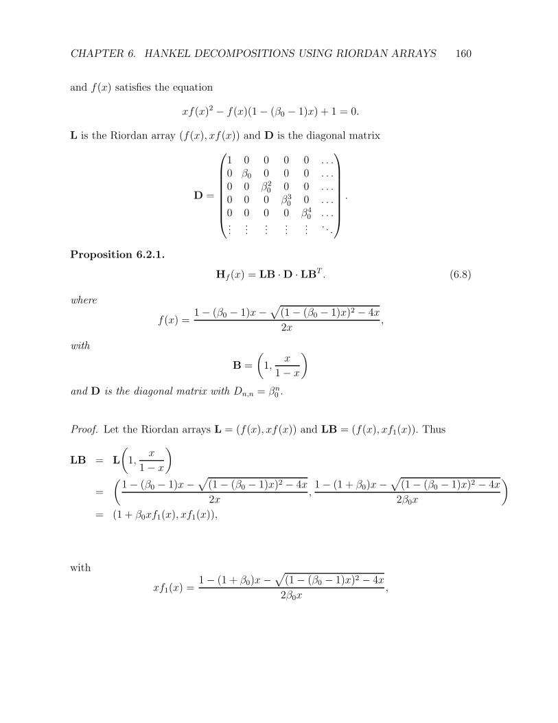
CHAPTER 6. HANKEL DECOMPOSITIONS USING RIORDAN ARRAYS 160
and f(x) satisfies the equation
xf(x)2 − f(x)(1 − (β0 − 1)x) + 1 = 0.
L is the Riordan array (f(x), xf(x)) and D is the diagonal matrix
D =
1 0 0 0 0 . . .0 β0 0 0 0 . . .0 0 β2
0 0 0 . . .0 0 0 β3
0 0 . . .0 0 0 0 β4
0 . . ....
......
......
. . .
.
Proposition 6.2.1.
Hf(x) = LB · D · LBT . (6.8)
where
f(x) =1 − (β0 − 1)x−
√
(1 − (β0 − 1)x)2 − 4x
2x,
with
B =
(
1,x
1 − x
)
and D is the diagonal matrix with Dn,n = βn0 .
Proof. Let the Riordan arrays L = (f(x), xf(x)) and LB = (f(x), xf1(x)). Thus
LB = L
(
1,x
1 − x
)
=
(
1 − (β0 − 1)x−√
(1 − (β0 − 1)x)2 − 4x
2x,
1 − (1 + β0)x−√
(1 − (β0 − 1)x)2 − 4x
2β0x
)
= (1 + β0xf1(x), xf1(x)),
with
xf1(x) =1 − (1 + β0)x−
√
(1 − (β0 − 1)x)2 − 4x
2β0x,

CHAPTER 6. HANKEL DECOMPOSITIONS USING RIORDAN ARRAYS 161
which satisfies the equation
β0x(xf1(x))2 + (xf1(x))(x(1 + β0) − 1) + x = 0.
Now, we can rewrite LB as(
1
1 − β0x− β0x(xf1(x)),
x
1 − (β0 + 1)x− β0x(xf1(x))
)
.
This satisfies Theorem 6.1.1 with associated Stieltjes matrix
SLB =
β0 1 0 0 . . .
β0 β0 + 1 1 0 . . .
0 β0 β0 + 1 1 . . .
0 0 β0 β0 + 1 . . ....
......
. . .
,
thus eq. (6.8) is also satisfied.
Corollary 6.2.2. The nth Hankel transform of an = [xn]f(x) where Hf satisfies eq.
(6.8) is βn(n+1)
20 .
Investigating the form of the Hankel matrix formed from the sequence of coefficientsof the series reversion of
xf(x) =1 − (β0 − 1)x−
√
(1 − (β0 − 1)x)2 − 4x
2,
we let
xg(x) = Rev(xf(x)) =x(1 − x)
1 + (β0 − 1)x
and find for the form of the Hankel matrix Hg, that we have the decomposition
Hg = L−1M · D · (L−1M)T (6.9)
where M is the matrix with first column 0n and second column with g.f.
xf(x) =1 − (1 + β0)x−
√
(1 − (β0 − 1)x)2 − 4x
2β0x.

CHAPTER 6. HANKEL DECOMPOSITIONS USING RIORDAN ARRAYS 162
All other columns are zero.
Now, let us look at some examples of g.f.’s that satisfy Theorem 6.8 above.
Example. Let L = (f(x), xf(x)), where
f(x) =1
1 − xf(x),
is the g.f. of the sequence of Catalan numbers (A000108 ). Two continued fraction
forms of the g.f. of the Catalan numbers are
f(x) =1
1 −x
1 −x
1 −x
. . .
=1
1 − x−x2
1 − 2x−x2
1 − 2x−x2
. . .
.
Now, we have Hf = LB · (LB)T , the first few rows of this matrix equation expand as
1 0 0 0 . . .
1 1 0 0 . . .
2 2 1 0 . . .
5 5 3 1 . . ....
......
. . .
1 0 0 0 . . .
0 1 0 0 . . .
0 1 1 0 . . .
0 1 2 1 . . ....
......
. . .
1 0 0 0 . . .
0 1 0 0 . . .
0 1 1 0 . . .
0 1 2 1 . . ....
......
. . .
T
1 0 0 0 . . .
1 1 0 0 . . .
2 2 1 0 . . .
5 5 3 1 . . ....
......
. . .
T
.

CHAPTER 6. HANKEL DECOMPOSITIONS USING RIORDAN ARRAYS 163
The associated Stieltjes matrices of L and LB are
SL =
1 1 0 0 . . .
1 1 1 0 . . .
1 1 1 1 . . .
1 1 1 1 . . ....
......
. . .
,
which are the Lukasiewicz paths with weight of one for all E and S-E steps, and
SLB =
1 1 0 0 . . .
1 2 1 0 . . .
0 1 2 1 . . .
0 0 1 2 . . ....
......
. . .
which are the Motzkin paths with weight of one for all S-E steps and weight of two for
all E steps, except the x-axis E step, which has weight one.
We note that L−1 = (g(x), xg(x)) =(
1 − x, x(1 − x))
and Hg = L−1M · D · (L−1M)T
expands as
1 0 0 . . .
−1 1 0 . . .
0 −2 1 . . .
0 1 −3 . . ....
.... . .
1 0 0 . . .
0 1 0 . . .
0 2 0 . . .
0 5 0 . . ....
.... . .
1 0 0 . . .
0 −1 0 . . .
0 0 −1 . . .
0 0 0 . . ....
.... . .
1 0 0 . . .
0 1 0 . . .
0 2 0 . . .
0 5 0 . . ....
.... . .
T
1 0 0 . . .
−1 1 0 . . .
0 −2 1 . . .
0 1 −3 . . ....
.... . .
T
.
Example. Let L = (f(x), xf(x)) where f(x) satisfies the equation
f(x)2x− f(x)(1 − x) + 1 = 0,

CHAPTER 6. HANKEL DECOMPOSITIONS USING RIORDAN ARRAYS 164
with
f(x) =1 − x−
√x2 − 6x + 1
2x,
which is the g.f. of the sequence of the large Schroder numbers,(A006318). Two forms
of the continued fraction expansion of f(x) are given by
f(x) =1
1 − x−x
1 − x−x
1 − x−x
. . .
=1
1 − 2x−2x2
1 − 3x−2x2
1 − 3x−2x2
. . .
.
Now, Hf = LB · D · (LB)T , which expands as
1 0 0 0 . . .
2 1 0 0 . . .
6 4 1 0 . . .
22 16 6 1 . . ....
......
. . .
1 0 0 0 . . .
0 1 0 0 . . .
0 1 1 0 . . .
0 1 2 1 . . ....
......
. . .
1 0 0 0 . . .
0 2 0 0 . . .
0 0 4 0 . . .
0 0 0 8 . . ....
......
.... . .
1 0 0 0 . . .
0 1 0 0 . . .
0 1 1 0 . . .
0 1 2 1 . . ....
......
. . .
T
1 0 0 0 . . .
2 1 0 0 . . .
6 4 1 0 . . .
22 16 6 1 . . ....
......
. . .
T
.
The associated Stieltjes matrices of L and LB are,
SL =
2 1 0 0 0 . . .
2 2 1 0 0 . . .
2 2 2 1 0 . . .
2 2 2 2 1 . . ....
......
.... . .
,

CHAPTER 6. HANKEL DECOMPOSITIONS USING RIORDAN ARRAYS 165
which are the Lukasiewicz paths with weight of two for all E and S-E steps, and
SLB =
2 1 0 0 . . .
2 3 1 0 . . .
0 2 3 1 . . .
0 0 2 3 . . ....
......
. . .
,
which are the Motzkin paths with weight of two for all S-E steps and weight of three for
all E steps, except the x-axis E step which has weight two.
We note that L−1 = (g(x), xg(x)) =
(
1−x1+x
, x(1−x)1+x
)
. Hg = L−1M ·D · (L−1M)T expands
as
1 0 0 . . .
−2 1 0 . . .
2 −4 1 . . .
−2 8 −6 . . ....
.... . .
1 0 0 . . .
0 1 0 . . .
0 3 0 . . .
0 11 0 . . ....
.... . .
1 0 0 . . .
0 −2 0 . . .
0 0 −2 . . .
0 0 0 . . ....
.... . .
1 0 0 . . .
0 1 0 . . .
0 3 0 . . .
0 11 0 . . ....
.... . .
T
1 0 0 . . .
−2 1 0 . . .
2 −4 1 . . .
−2 8 −6 . . ....
.... . .
T
.
Example. Let L = (f(x), xf(x)), where f(x) satisfies the equation
f(x)2x− f(x)(1 − 2x) + 1 = 0
with
f(x) =1 − 2x−
√4x2 − 8x + 1
2x,
which is the g.f. of the sequence of planar rooted trees with n nodes and tricolored end

CHAPTER 6. HANKEL DECOMPOSITIONS USING RIORDAN ARRAYS 166
nodes (A047891). Two continued fraction expansions of the g.f. have the form,
f(x) =1
1 − 2x−x
1 − 2x−x
1 − 2x−x
. . .
=1
1 − 3x−3x2
1 − 4x−3x2
1 − 4x−3x2
. . .
.
We have Hf = LB · D · (LB)T which expands as
1 0 0 0 . . .
3 1 0 0 . . .
12 6 1 0 . . .
57 33 9 1 . . ....
......
. . .
1 0 0 0 . . .
0 1 0 0 . . .
0 1 1 0 . . .
0 1 2 1 . . ....
......
. . .
1 0 0 0 . . .
0 3 0 0 . . .
0 0 9 0 . . .
0 0 0 27 . . ....
......
.... . .
1 0 0 0 . . .
0 1 0 0 . . .
0 1 1 0 . . .
0 1 2 1 . . ....
......
. . .
T
1 0 0 0 . . .
3 1 0 0 . . .
12 6 1 0 . . .
57 33 9 1 . . ....
......
. . .
T
.
The associated Stieltjes matrices of L and LB are
SL =
3 1 0 0 0 . . .
3 3 1 0 0 . . .
3 3 3 1 0 . . .
3 3 3 3 1 . . ....
......
.... . .
,
which are the Lukasiewicz paths with weight three for all E and S-E steps, and
SLB =
3 1 0 0 . . .
3 4 1 0 . . .
0 3 4 1 . . .
0 0 3 4 . . ....
......
. . .

CHAPTER 6. HANKEL DECOMPOSITIONS USING RIORDAN ARRAYS 167
which are the Motzkin paths with weight of three for all S-E steps and weight of four
for all E steps, except the x-axis E step which has weight three.
We note that L−1 = (g(x), xg(x)) =
(
1−x1+2x
, x(1−x)1+2x
)
. Hg = L−1M·D·(L−1M)T expands
as
1 0 0 . . .
−3 1 0 . . .
6 −6 1 . . .
−12 21 −9 . . ....
.... . .
1 0 0 . . .
0 1 0 . . .
0 2 0 . . .
0 4 0 . . ....
.... . .
1 0 0 . . .
0 −3 0 . . .
0 0 −3 . . .
0 0 0 . . ....
.... . .
1 0 0 . . .
0 1 0 . . .
0 2 0 . . .
0 4 0 . . ....
.... . .
T
1 0 0 . . .
−3 1 0 . . .
6 −6 1 . . .
−12 21 −9 . . ....
.... . .
T
.
Corollary 6.2.3. A bijection exists between Lukasiewicz paths with weight α for all E
and S-E steps, where the first few elements of the associated Stieltjes matrix expand as
α 1 0 0 0 . . .
α α 1 0 0 . . .
α α α 1 0 . . .
α α α α 1 . . ....
......
.... . .
and Motzkin paths with weight of α for all S-E steps and weight of α+1 for all E steps,
except the x-axis E step which has weight α. The first few elements of the associated
Stieltjes expand as
α 1 0 0 . . .
α α + 1 1 0 . . .
0 α α + 1 1 . . .
0 0 α α + 1 . . ....
......
. . .
.
Proof. Proof follows from eq. (6.8).

CHAPTER 6. HANKEL DECOMPOSITIONS USING RIORDAN ARRAYS 168
We now turn our attention to Riordan arrays L = (g(x), xf(x)) with g(x) 6= f(x) andwe introduce the following proposition. In terms of paths, we will now look at pathswhere the weights of the steps returning to the x-axis, or level steps on the x-axis differfrom the other possible steps of the paths considered.
Proposition 6.2.4.
Hg(x) = LB · D · LBT ,
where the Riordan array
L = (g(x), xf(x)) =
(
1
1 − (β0 − α0
β1)x− α0
β1xf(x)
,x
(1 − (β1 − 1)x) − xf(x)
)
(6.10)
with
xf(x) =1 − (β1 − 1)x−
√
(1 − (β1 − 1)x)2 − 4x
2,
and L has the associated Stieltjes matrix
SL =
β0 1 0 0 . . .
α0 β1 1 0 . . .
α0 β1 β1 1 . . .
α0 β1 β1 β1 . . ....
......
. . .
.
We note that following the notation of the Stieltjes matrix above, S-E steps returningto the axis have the same weight, α0 with E steps on the x-axis having weight β0. Allother S-E and E steps have weight β1.
Proof. Now for LB = (g(x), xf1(x)), with L = (g(x), xf(x)) we have the Riordan array
L
(
1,x
1 − x
)
=
(
1
1 − (β0 − α0
β1)x− α0
β1xf(x)
,1 − (1 + β1)x−
√
(1 − (β1 − 1)x)2 − 4x
2β1
)
.
As xf1(x) =1−(1+β1)x−
√(1−(β1−1)x)2−4x
2β1we can rewrite LB as
(
1
1 − β0x− α0x2f1(x), xf1(x)
)
,

CHAPTER 6. HANKEL DECOMPOSITIONS USING RIORDAN ARRAYS 169
which has associated Stieltjes matrix
SLB =
β0 1 0 0 . . .
α0 β1 + 1 1 0 . . .
0 β1 β1 + 1 1 . . .
0 0 β1 β1 + 1 . . ....
......
. . .
.
We can rewrite
LB =
(
1
1 − β0x− α0x(xf1(x)),
x
1 − (β1 + 1)x− β1x(xf1(x))
)
.
The Riordan array above satisfies Theorem 6.1.1, thus
Hg(x) = LB · D · LBT .
Example. We consider the g.f. with continued fraction expansion
1
1 − x−2x
1 −x
1 −x
. . .
,
which is the g.f. of the sequence (A026671).
The associated Stieltjes matrices of L and LB are
SL =
3 1 0 0 . . .
2 1 1 0 . . .
2 1 1 1 . . .
2 1 1 1 . . ....
......
. . .
,

CHAPTER 6. HANKEL DECOMPOSITIONS USING RIORDAN ARRAYS 170
which are the Lukasiewicz paths with weight of one for all E and S-E steps except those
returning to the x-axis, when the E step has weight three and the S-E steps have weight
two, and
SLB =
3 1 0 0 . . .
2 2 1 0 . . .
0 1 2 1 . . .
0 0 1 2 . . ....
......
. . .
which are the Motzkin paths with weight of one for all S-E steps and weight of two for
all E steps, except the x-axis E step which has weight three and the S-E step returning
to the x-axis has weight of two.
6.2.1 Binomial transforms
Now, as the Hankel transform is invariant under the Binomial transform [78], we areinterested in the form of the Binomial transform of the generating functions above.Firstly let us look at generating functions of the form in eq. (6.8), that satisfy theequation
xf(x)2 − f(x)(1 − (β1 − 1)x) + 1 = 0.
We have the following proposition
Proposition 6.2.5. An o.g.f. which satisfies
x(1 − βx)f(x)2 − f(x)(1 − (β1 − 1 + β)x) + 1 = 0 (6.11)

CHAPTER 6. HANKEL DECOMPOSITIONS USING RIORDAN ARRAYS 171
with continued fraction expansion of f(x)
f(x) =1
1 − (β1 − 1 + β)x−x(1 − βx)
1 − (β1 − 1 + β)x−x(1 − βx)
1 − (β1 − 1 + β)x−x(1 − βx)
. . .
has related Stieltjes matrix
β + β1 1 0 0 . . .
β1 β + β1 1 0 . . .
β1 β1 β + β1 1 . . .
β1 β1 β1 β + β1 . . ....
......
. . .
.
Proof. Applying proposition 2.4.8 to the Riordan array (f(x), xf(x)), where xf(x) is
xf(x) =x
1 − (β1 − 1 + β)x− (1 − βx)xf(x),
gives the required result.
Corollary 6.2.6. The βth binomial transform of the Riordan array (fβ(x), xfβ(x))
with f(x) satisfying
xf(x)2 − f(x)(1 − (β1 − 1)x) + 1 = 0
satisfies
x(1 − βx)fβ(x)2 − fβ(x)(1 − (β1 − 1 + β)x) + 1.
Example. For β1 = 2 we have
xf(x)2 − f(x)(1 − x) + 1 = 0

CHAPTER 6. HANKEL DECOMPOSITIONS USING RIORDAN ARRAYS 172
with
f(x) =x− 1 +
√x2 − 6x + 1
−2x.
The g.f. f(x) has a continued fraction expansion
1
(1 − x) −x
(1 − x) −x
(1 − x) −x
. . .
,
which is the g.f. for the sequence of the large Schroeder numbers (A006318). The
Hankel matrix decomposes as
1 0 0 0 . . .
2 1 0 0 . . .
6 4 1 0 . . .
22 16 6 1 . . ....
......
. . .
1 0 0 0 . . .
0 1 0 0 . . .
0 1 1 0 . . .
0 1 2 1 . . ....
......
. . .
1 0 0 0 . . .
0 2 0 0 . . .
0 0 4 0 . . .
0 0 0 8 . . ....
......
. . .
1 0 0 0 . . .
0 1 0 0 . . .
0 1 1 0 . . .
0 1 2 1 . . ....
......
. . .
T
1 0 0 0 . . .
2 1 0 0 . . .
6 4 1 0 . . .
22 16 6 1 . . ....
......
. . .
T
so hn = 2n(n+1)
2 is the nth Hankel transform with first few elements
1, 2, 8, 64, 1024, . . . (A006125).
Now, the binomial transform, (g1(x), xf1(x)), with β = 1 satisfies,
x(1 − x)f1(x)2 − f1(x)(1 − 2x) + 1 = 0
with
f1(x) =2x− 1 +
√8x2 − 8x + 1
2x(x− 1),

CHAPTER 6. HANKEL DECOMPOSITIONS USING RIORDAN ARRAYS 173
and f1(x) has a continued fraction expansion
1
(1 − 2x) −x(1 − x)
(1 − 2x) −x(1 − x)
(1 − 2x) −x(1 − x)
. . .
,
which is the g.f. for the sequence (A174347).
Now we look at g.f.’s of the form where g(x) 6= f(x), and the Riordan array L =(
g(x), xf(x))
has
g(x) =1
1 − (β + β1)x− x(1 − βx)f(x), f(x) =
1
1 − (β + β0)x− x(1 − βx)f(x).
In terms of paths, all E and S-E steps have the same weighting, except for that of theE step on the x-axis.
The associated Stieltjes matrix has the form
β + β1 1 0 0 . . .β0 β + β0 1 0 . . .β0 β0 β + β0 1 . . .β0 β0 β0 β + β0 . . ....
......
. . .
.
The g.f. of g1(x), the g.f. of the first row of the Riordan array after multiplication ofthe Binomial array, has a continued fraction expansion
1
1 − (β + β1 − 1)x− x(1 − βx)
1 − (β0 − 1 + β)x− x(1 − βx)
1 − (β0 − 1 + β)x− x(1 − βx)
. . .
.

CHAPTER 6. HANKEL DECOMPOSITIONS USING RIORDAN ARRAYS 174
We note that
L−1 =
(
x2(β0 − β1) − x(β0 − β1 − 1) − 1
x2β − x(β + β0) − 1,
x(x− 1)
βx2 − x(β + β0) − 1
)
.
Let us look at some examples of Riordan arrays of the above form.
Example. For β0 = 0, β1 = 2 with β = 0, 1, 2 ,
g(x) =1
1 − 2x− xf(x)
and g(x) has a continued fraction expansion
1
1 − 2x−x
1 −x
1 − x . . .
.
The coefficients of the related power series form the sequence (A001700). Note that for
L = (g(x), xf(x)) then
L−1 = (2x2 − 3x + 1, x(1 − x)).
The Binomial transform of g(x) is
g1(x) =1
1 − 3x− x(1 − x)f(x)
and g1(x) has a continued fraction expansion
1
1 − 3x−x(1 − x)
1 − x−x(1 − x)
1 − x− x(1 − x) . . .
.

CHAPTER 6. HANKEL DECOMPOSITIONS USING RIORDAN ARRAYS 175
The coefficients of the related power series form the sequence (A026378). If L1 =
(g1(x), xf1(x)) then the Riordan array
L1−1 =
(−(2x2 − 3x + 1)
x2 − x− 1,x(x− 1)
x2 − x− 1
)
.
Rev(xf1(x)) are the alternating signed Fibonacci numbers. The second Binomial trans-
form (g2(x), xf2(x)), with β = 2, has
g2(x) =1
1 − 4x− x(1 − 2x)f(x),
and g2(x) has a continued fraction expansion
1
1 − 4x−(1 − 2x)x
1 − 2x−(1 − 2x)x
1 − 2x− x(1 − 2x) . . .
.
The coefficients of the related power series form the sequence (A005573).
L2−1 = ((g2(x), xf2(x)))−1 =
(−(2x2 − 3x + 1)
2x2 − 2x− 1,
x(x− 1)
2x2 − 2x− 1
)
where Rev(xf2(x)) is the sequence A028859. In general, the related Stieltjes matrices
for each of the β values above is
2 + β 1 0 0 . . .
1 1 + β 1 0 . . .
1 1 1 + β 1 . . .
1 1 1 1 + β . . ....
......
. . .
,
where the related Lukasiewicz paths have weight one for all the S-E steps, and weight
β for all E steps, except those E steps on the x-axis, where they have weight β + 2.

CHAPTER 6. HANKEL DECOMPOSITIONS USING RIORDAN ARRAYS 176
Now finally we turn our attention to the binomial transforms of g.f.’s of the form ineq. (6.12) where g(x) 6= f(x), and the Riordan array L =
(
g(x), xf(x))
has the form
(
1
1 − (β0 − α0
β1)x− α0
β1xf(x)
,x
(1 − (β1 − 1)x) − xf(x)
)
.
Here, we have the binomial transform
(
1
1 − (β0 − α0
β1+ β)x− α0
β1(1 − β)xf(x)
,x
(1 − (β1 − 1)x) − x(1 − β)f(x)
)
.
Example. We look at the first binomial transform of the g.f.
1
1 − x−2x
1 −x
1 −x
. . .
,
which is the g.f. for the sequence(A026671). The associated Stieltjes matrix is
3 1 0 0 . . .
2 1 1 0 . . .
2 1 1 1 . . .
2 1 1 1 . . ....
......
. . .
,
with related Lukasiewicz paths with E and S-E steps all of weight one except for E steps
on the x-axis having weight three and S-E steps returning to the x-axis having weight

CHAPTER 6. HANKEL DECOMPOSITIONS USING RIORDAN ARRAYS 177
two. We have a continued fraction expansion for the binomial transform
1
1 − 2x−2x(1 − x)
1 − x−x(1 − x)
1 − x−x(1 − x)
. . .
,
which is the g.f. of the sequence (A026671), with corresponding Stieltjes matrix
4 1 0 0 . . .
2 2 1 0 . . .
2 1 2 1 . . .
2 1 1 2 . . ....
......
. . .
,
which has the same steps as the Stieltjes above, excepts for an increase of the weight of
one for each of the level steps.
As we noted in section 5.1.1 where we constructed the binomial transform of a Motzkinpath, a bijection between a Motzkin and Lukasiewicz path is preserved under thebinomial transform. We refer the reader to section 5.4, where we have constructed onesuch bijection satisfying the g.f.’s from this section, where the related Stieltjes matriceshave the form
SL =
0 1 0 0 . . .1 0 1 0 . . .1 1 0 1 . . .1 1 1 0 . . ....
......
. . .
,
which are the Lukasiewicz paths with weight of one for all S-E steps and no E steps

CHAPTER 6. HANKEL DECOMPOSITIONS USING RIORDAN ARRAYS 178
permitted, and
SLB =
0 1 0 0 . . .1 1 1 0 . . .0 1 1 1 . . .0 0 1 1 . . ....
......
. . .
,
which are the Motzkin paths with weight of one for all steps except no E steps permittedon the x-axis. We note that this is the inverse binomial transform of the g.f. fromexample 6.2.
6.3 A second Hankel matrix decomposition
Finally before we leave this chapter we naturally lead ourselves to consider a similardecomposition as in eq. (6.8), where we look at the Riordan array decompositioninvolving the inverse of the “shifted binomial” matrix B, as defined in the last section.This inspires the last section in this chapter. We note that we do not consider relatedlattice paths in this last section as the form of the Stieltjes matrix does not correspondto any paths that we have previously encountered. Once again, we will also look at thebinomial transforms of Riordan arrays satisfying our new Riordan array decomposition,and again we will consider the form of their associated Stieltjes matrices.
We now introduce the following decomposition of a Hankel matrix Hg :
Hg = L−1M · D · (L−1M)T , (6.12)
where the Hankel matrix Hg is the matrix where an = [xn]g(x) and L is the Riordanarray (g(x), xg(x)), where
g(x) =(1 + nx)
1 + (2n + β)x + (n2 + βn + 1)x2, (6.13)
with β > 0, D a diagonal matrix, and M the matrix with first column 0n and secondcolumn equal to Rev(xg(x)), where
Rev(xg(x)) = xf(x) =x
1 − (2n + β)x + (n− (n2 + βn + 1)x)xf(x)(6.14)
=
√
x2(β2 − 4) − 2xβ + 1 + x(β + 2n) − 1
2(n− x(βn + n2 + 1)). (6.15)

CHAPTER 6. HANKEL DECOMPOSITIONS USING RIORDAN ARRAYS 179
We will see in the examples below that the Hankel matrix Hf , with an = [xn]f(x)
where f(x) is the g.f. of the series reversion of g(x), decomposes into LB−m · LB−mT,
for some m, where L = (f(x), xf(x)) and B = (1, 11+x
), so so we have the following,
(f(x), xf(x))
(
1,x
1 + nx
)
=
(
1,x
1 + nx
)
=
(
f(x),xf(x)
1 + n(xf(x))
)
.
Now xf(x)1+n(xf(x))
simplifies to
1 − βx−√
x2(β2 − 4) − 2xβ + 1
2x,
giving the Riordan array (g(x), xf(x)):
(
√
x2(β2 − 4 − 2xβ + 1) + x(β + 2n) − 1
2(n− x(βn + n2 + 1)),
1 − βx−√
x2(β2 − 4) − 2xβ + 1
2x
)
which is the Riordan array
(
1
1 − (β + n)x− x(xf(x)), xf(x)
)
,
which has a corresponding tridiagonal Stieltjes matrices.
Let us look at some examples. Note that as the g.f.’s of the Riordan arrays depend ontwo variables, we will use the notation L = Ln,β for the rest of this section.
Example. For β = 1, MDM has the form
1 0 0 0 . . .
0 1 0 0 . . .
0 1 0 0 . . .
0 2 0 0 . . ....
......
. . .
1 0 0 0 . . .
0 −1 0 0 . . .
0 0 −1 0 . . .
0 0 0 −1 . . ....
......
. . .
1 0 0 0 . . .
0 1 0 0 . . .
0 1 0 0 . . .
0 2 0 0 . . ....
......
. . .
T
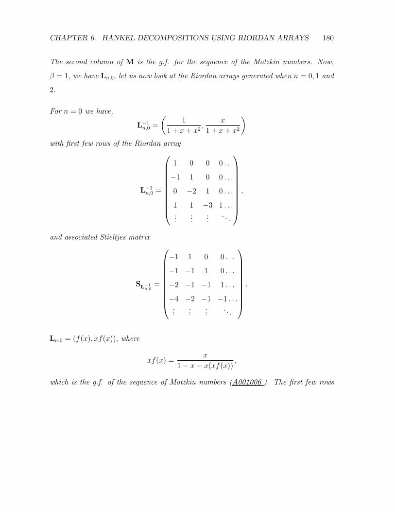
CHAPTER 6. HANKEL DECOMPOSITIONS USING RIORDAN ARRAYS 180
The second column of M is the g.f. for the sequence of the Motzkin numbers. Now,
β = 1, we have Ln,0, let us now look at the Riordan arrays generated when n = 0, 1 and
2.
For n = 0 we have,
L−1n,0 =
(
1
1 + x + x2,
x
1 + x + x2
)
with first few rows of the Riordan array
L−1n,0 =
1 0 0 0 . . .
−1 1 0 0 . . .
0 −2 1 0 . . .
1 1 −3 1 . . ....
......
. . .
,
and associated Stieltjes matrix
SL−1n,0
=
−1 1 0 0 . . .
−1 −1 1 0 . . .
−2 −1 −1 1 . . .
−4 −2 −1 −1 . . ....
......
. . .
.
Ln,0 = (f(x), xf(x)), where
xf(x) =x
1 − x− x(xf(x)),
which is the g.f. of the sequence of Motzkin numbers (A001006 ). The first few rows

CHAPTER 6. HANKEL DECOMPOSITIONS USING RIORDAN ARRAYS 181
of the Riordan array expand as
Ln,0 =
1 0 0 0 . . .
1 1 0 0 . . .
2 2 1 0 . . .
4 5 3 1 . . ....
......
. . .
,
with associated Stieltjes matrix
SLn,0 =
1 1 0 0 . . .
1 1 1 0 . . .
0 1 1 1 . . .
0 0 1 1 . . ....
......
. . .
.
We note that (Ln,0) · (LTn,0) = H.
For n = 1 we have
L−1n,1 =
(
1 + x
1 + 3x + 3x2,
x(1 + x)
1 + 3x + 3x2
)
,
with first few rows of the Riordan array
L−1n,1 =
1 0 0 0 . . .
−2 1 0 0 . . .
3 −4 1 0 . . .
−3 10 −6 1 . . ....
......
. . .
,

CHAPTER 6. HANKEL DECOMPOSITIONS USING RIORDAN ARRAYS 182
with associated Stieltjes matrix
SL−1n,1
=
−2 1 0 0 . . .
−1 −2 1 0 . . .
−2 −1 −2 1 . . .
−4 −2 −1 −2 . . ....
......
. . .
.
Ln,1 = (f(x), xf(x)), where
xf(x) =x
1 − 3x + (xf(x))(1 − 3x),
which is the g.f. of the sequence of numbers of directed animals of size n (A005773),
with first few rows of the Riordan array
Ln,1 =
1 0 0 0 . . .
2 1 0 0 . . .
5 4 1 0 . . .
13 14 6 1 . . ....
......
. . .
,
and associated Stieltjes matrix,
SLn,1 =
2 1 0 0 . . .
1 2 1 0 . . .
−1 1 2 1 . . .
1 −1 1 2 . . ....
......
. . .
.
We note that Ln,1(B−1) · (Ln,1(B
−1))T = Hf . The first few rows of Ln,1(B−1) expand

CHAPTER 6. HANKEL DECOMPOSITIONS USING RIORDAN ARRAYS 183
as,
1 0 0 0 . . .
2 1 0 0 . . .
5 4 1 0 . . .
13 14 6 1 . . ....
......
. . .
1 0 0 0 . . .
0 1 0 0 . . .
0 −1 1 0 . . .
0 1 −2 1 . . ....
......
. . .
=
1 0 0 0 . . .
2 1 0 0 . . .
5 3 1 0 . . .
13 9 4 1 . . ....
......
. . .
,
with associated Stieltjes matrix,
SLn,1(B−1) =
2 1 0 0 . . .
1 1 1 0 . . .
0 1 1 1 . . .
0 0 1 1 . . ....
......
. . .
.
Finally, for n = 2 we have
L−1n,2 =
(
1 + 2x
1 + 5x + 7x2,
x(1 + 2x)
1 + 5x + 7x2
)
,
with first few rows of the Riordan array
L−1n,2 =
1 0 0 0 . . .
−3 1 0 0 . . .
8 −6 1 0 . . .
−19 25 −9 1 . . ....
......
. . .
,

CHAPTER 6. HANKEL DECOMPOSITIONS USING RIORDAN ARRAYS 184
and associated Stieltjes matrix,
SL−1n,2
=
−3 1 0 0 . . .
−1 −3 1 0 . . .
−2 −1 −3 1 . . .
−4 −2 −1 −3 . . ....
......
. . .
.
Ln,2 = (f(x), xf(x)), where
xf(x) =x
1 − 5x + (xf(x))(2 − 7x),
which is the g.f. for the sequence (A059738). The Riordan array has first few rows
Ln,2 =
1 0 0 0 . . .
3 1 0 0 . . .
10 6 1 0 . . .
34 29 9 1 . . ....
......
. . .
,
and associated Stieltjes matrix,
SLn,2 =
3 1 0 0 . . .
1 3 1 0 . . .
−2 1 3 1 . . .
4 −2 1 3 . . ....
......
. . .
.

CHAPTER 6. HANKEL DECOMPOSITIONS USING RIORDAN ARRAYS 185
We have Ln,2(B−2) · (Ln,2(B
−2))T = Hf
Ln,2(B−2) =
1 0 0 0 . . .
3 1 0 0 . . .
10 6 1 0 . . .
34 29 9 1 . . ....
......
. . .
1 0 0 0 . . .
0 1 0 0 . . .
0 −1 1 0 . . .
0 1 −2 1 . . ....
......
. . .
2
=
1 0 0 0 . . .
3 1 0 0 . . .
10 4 1 0 . . .
34 15 5 1 . . ....
......
. . .
,
with associated Stieltjes matrix,
SLn,2B−2 =
3 1 0 0 . . .
1 1 1 0 . . .
0 1 1 1 . . .
0 0 1 1 . . ....
......
. . .
.
Now, we have seen some examples above of Stieltjes matrices related to generatingfunctions of the form in eq. (6.15). From eq. (4.7) in proposition 4.3.2 we saw thatthe rows of the Stieltjes matrix corresponding to the Riordan array (g(x), xg(x)) of theBell subgroup have the form
A(x) =x
xg(x)and Z(x) =
1
xg(x)− 1
x.
Using this result, we have the following
Corollary 6.3.1. The Stieltjes matrix of the Riordan array (f(x), xf(x)) where
xf(x) =x
1 − (2n + β)x + (n− (n2 + βn + 1)x)f(x)
is formed by the power series
A(x) = 1 + (β + n)x + x2∞∑
m=0
(−n)mxm+2

CHAPTER 6. HANKEL DECOMPOSITIONS USING RIORDAN ARRAYS 186
and
Z(x) = (β + n)x + x2
∞∑
m=0
(−n)mxm+2
Proof. The rows of the Stieltjes matrix corresponding to the Riordan array (f(x), xf(x))
of the Bell subgroup have the form
A(x) =x
xf(x)and Z(x) =
1
xf(x)− 1
x.
From eq. (6.13) we have the series reversion of xf(x)
rev(xf(x)) = xg(x) =(1 + nx)x
(1 + (2n + β)x + (n2 + βn + 1)x2).
We have
A(x) =(1 + (2n + β)x + (n2 + βn + 1)x2)
(1 + nx)= 1 + (β + n)x + x2
∞∑
m=0
(−n)mxm+2,
and
Z(x) =(1 + (2n + β)x + (n2 + βn + 1)x2)
(1 + nx)x− 1
x= (β + n)x + x2
∞∑
m=0
(−n)mxm+2
Now, we note that the g.f. from eq. (6.12)
g(x) =(1 + nx)
1 + (2n + β)x + (n2 + βn + 1)x2
can be rewritten in the form
1
1 + (n + β)x + x2
1+nx
.
In the table in Fig. (6.3) below we see that for each β, the functions
g(x) =(1 + nx)
1 + (2n + β)x + (n2 + βn + 1)x2

CHAPTER 6. HANKEL DECOMPOSITIONS USING RIORDAN ARRAYS 187
are successive inverse transforms for increasing n and for the series reversion,
Rev(xg(x)) = xf(x) =x
1 − (2n + β)x + (n− (n2 + βn + 1)x)xf(x)
=
√
x2(b2 − 4) − 2xb + 1 + x(b + 2n) − 1
2(n− x(βn + n2 + 1))
for each value of n the functions xf(x) are successive binomial transforms for increasingvalues of β. This leads us to the final proposition in this chapter:
Proposition 6.3.2. The inverse binomial transform of
g(x) =(1 + nx)
1 + (2n + β)x + (n2 + βn + 1)x2=
1
1 + (n + β)x + x2
1+nx
,
is1
1 + (n + 1 + β)x +x2
1 + (n + 1)x
,
and the binomial tranform of
Rev(xg(x)) = xf(x) =x
1 − (2n + β)x + (n− (n2 + βn + 1)x)xf(x)
isx
1 − (2n + (β + 1))x + (n− (n2 + (β + 1)n + 1)x)xf(x)
Proof. Using Riordan arrays we proceed by showing that left multiplication of g(x) by

CHAPTER 6. HANKEL DECOMPOSITIONS USING RIORDAN ARRAYS 188
the inverse of the Binomial Riordan array gives the required g.f. That is
(
1
1 + x,
x
1 + x
)
1
1 + (n + β)x +x2
1 + nx
=1
1 + x
1
1 + (n + β)(
x1+x
)
+
(
x1+x
)2
1 + n(
x1+x
)
=1
1 + x
1 +nx
1 + x
1 +nx
1 + x+
x(n + β)
1 + x+
nx2(n + β)
(1 + x)2+
x
(1 + x)2
=1 + x(1 + n)
1 + x(1 + n) + (1 + x(1 + n))(n + 1 + β)x + x2
=1
1 + (n + 1 + β)x +x2
1 + (n + 1)x
.
For the series reversion f(x), we have
(
1
1 − x,
x
1 − x
)
√
x2(β2 − 4) − 2xβ + 1 + x(β + 2n) − 1
2(n− x(βn + n2 + 1))
=1
1 − x
√
(
x1−x
)2
(β2 − 4) − 2( x1−x
)β + 1 + ( x1−x
)(β + 2n) − 1
2( x1−x
)(n− ( x1−x
)(βn + n2 + 1))
=
√
x2(β2 − 4) − 2(x(1 − x))β + (1 − x)2 + x(β + 2n) − (1 − x)
2x(n(1 − x) − x(βn + n2 + 1))
=
√
x2((β + 1)2 − 4) − 2x(β + 1) + 1 + x((β + 1) + 2n) − 1
2(n− x(βn + n2 + 1))

CHAPTER 6. HANKEL DECOMPOSITIONS USING RIORDAN ARRAYS 189
β n = −1 n = 0 n = 1
1 g(x) =1
1 +x2
1− x
g(x) =1
1 + x+ x2
1
1 + 2x+x2
1 + x
1, 0,−1,−1, 0, 1, 1, . . . 1,−1, 0, 1,−1, 0, 1,−1, . . . 1,−2, 3,−3, 9, . . .
f(x) =1
1 + x+ (−1− x)f(x)f(x) =
1
1− x− xf(x)f(x) =
1
1− 3x+ (1− 3x)f(x)
1, 0, 1, 1, 3, 6, 15, . . . (A005043) 1, 1, 2, 4, 9, 21, . . . (A001006) 1, 2, 5, 13, 35, 96, . . . (A005773)
2 g(x) =1
1 + 1x+x2
1− x
g(x) =1
1 + 2x+ x2g(x) =
1
1 + 3x+x2
1 + x
1,−1, 0, 0, 0, . . . 1,−2, 3,−4, 5, . . . 1,−3, 8,−20 . . .
f(x) =1
1− f(x)f(x) =
1
1− 2x− xf(x)f(x) =
1
1− 4x+ (1− 4x)f(x)
1, 1, 2, 5, 14, 42, . . . (A000108) 1, 2, 5, 14, 42, . . . (A000108) 1, 3, 10, 35, 126, . . . (A001700)
3 g(x) =1
1 + 2x+x2
1− x
g(x) =1
1 + 3x+ x2g(x) =
1
1 + 4x+x2
1 + x
1,−2, 3,−5, 8,−13, 21, . . . 1,−3, 8,−21, 55,−144, . . . 1,−4, 15,−55, 200, . . .
f(x) =1
1− x+ (−1 + x)f(x)f(x) =
1
1− 3x− xf(x)f(x) =
1
1− 5x+ (1− 5x)f(x)
1, 2, 5, 15, 51, 188, . . . (A007317) 1, 3, 10, 36, . . . (A002212) 1, 4, 17, 75, 339, . . . (A026378)

Chapter 7
Narayana triangles
The Narayana numbers, which are closely related to the ubiquitous Catalan numbers,have an important and growing literature. Their applications are varied. In the nextchapter we will look at the mathematics of one application in the area of MIMO(multiple input, multiple output) wireless communication. For our purposes, it isuseful to distinguish between three different “Narayana triangles” and their associated“Narayana polynomials”. These triangles are documented separately in The On-lineEncyclopedia of Integer Sequences [124] along with other variants. We are interested inthe Hankel transform [78, 76] of a number of integer sequences that we shall encounter.Other areas where Narayana polynomials and their generalizations find applicationsinclude associahedra [23, 57, 105] and secondary RNA structures [43].
7.1 The Narayana Triangles and their generating
functions
In this section, we define four separate though related “Narayana triangles”, and wedescribe their (bivariate) generating functions.
190

CHAPTER 7. NARAYANA TRIANGLES 191
According to [166], the number triangle with general term
N0(n, k) =1
n + 0n
(
n
k
)(
n
k + 1
)
(7.1)
has g.f. φ0(x, y) which satisfies the equation
xyφ20 + (x + xy − 1)φ0 + x = 0.
Solving for φ0(x, y) yields
φ0(x, y) =1 − x(1 + y) −
√
1 − 2x(1 + y) + x2(1 − y)2
2xy. (7.2)
This triangle begins
N0 =
0 0 0 0 0 0 . . .1 0 0 0 0 0 . . .1 1 0 0 0 0 . . .1 3 1 0 0 0 . . .1 6 6 1 0 0 . . .1 10 20 10 1 0 . . ....
......
......
.... . .
.
The triangle N1 with general term
N1(n, k) = 0n+k +1
n + 0n
(
n
k
)(
n
k + 1
)
(7.3)
which begins
N1 =
1 0 0 0 0 0 . . .1 0 0 0 0 0 . . .1 1 0 0 0 0 . . .1 3 1 0 0 0 . . .1 6 6 1 0 0 . . .1 10 20 10 1 0 . . ....
......
......
.... . .
clearly has the g.f.
φ1(x, y) = 1 + φ0(x, y) =1 − x(1 − y) −
√
1 − 2x(1 + y) + x2(1 − y)2
2xy. (7.4)

CHAPTER 7. NARAYANA TRIANGLES 192
The triangle N2 with general term
N2(n, k) = [k ≤ n]N1(n, n− k) = 0n+k +1
n + 0nk
(
n
k
)(
n
k − 1
)
(7.5)
begins
N2 =
1 0 0 0 0 0 . . .0 1 0 0 0 0 . . .0 1 1 0 0 0 . . .0 1 3 1 0 0 . . .0 1 6 6 1 0 . . .0 1 10 20 10 1 . . ....
......
......
.... . .
.
This triangle has the g.f.
φ2(x, y) = 1 + yφ0(x, y) =1 + x(1 − y) −
√
1 − 2x(1 + y) + x2(1 − y)2
2x. (7.6)
Finally the “Pascal-like” variant N3 with general term
N3(n, k) = N0(n + 1, k) =1
n + 1
(
n + 1
k
)(
n + 1
k + 1
)
(7.7)
which begins
N3 =
1 0 0 0 0 0 . . .1 1 0 0 0 0 . . .1 3 1 0 0 0 . . .1 6 6 1 0 0 . . .1 10 20 10 1 0 . . .1 15 50 50 15 1 . . ....
......
......
.... . .
has the g.f.
φ3(x, y) =φ0(x, y)
x=
1 − x(1 + y) −√
1 − 2x(1 + y) + x2(1 − y)2
2x2y. (7.8)
Using the generating functions above, we can relate the Narayana triangles to theprocess of reverting sequences. We start by calculating the reversion of the expression
x(1 − xy)
1 − x(y − 1),

CHAPTER 7. NARAYANA TRIANGLES 193
considered as a function in x, with parameter y. This amounts to solving the equation
u(1 − uy)
1 − u(y − 1)= x
for the unknown u. We obtainu = xφ1(x, y).
Thus we have
φ1(x, y) =1
xRev
x(1 − xy)
1 − x(y − 1). (7.9)
In like manner, we obtain
φ2(x, y) =1
xRev
x(1 − x)
1 − x(1 − y)(7.10)
and
φ3(x, y) =1
xRev
x
1 + (1 + y)x + yx2. (7.11)
7.2 The Narayana Triangles and continued fractions
In this section, we develop continued fraction versions for each of the generating func-tions φ1, φ2, φ3.
It is easy to see that φ1(x, y) obeys the equation [21]
xyφ21 − (xy − x + 1)φ1 + 1 = 0. (7.12)
Thusφ1(1 − x− xyφ1) = 1 − xyφ1
and thus
φ1 =1 − xyφ1
1 − xyφ1 − x
=1
1 − x1−xyφ1
.

CHAPTER 7. NARAYANA TRIANGLES 194
We thus obtain the result that φ1(x, y) can be expressed as the continued fraction
φ1(x, y) =1
1 − x
1 − xy
1 − x
1 − xy
1 − · · ·
. (7.13)
Similarly for φ2(x, y), we have
xφ22 − (1 + x− xy)φ2 + 1 = 0 (7.14)
from which we deduceφ2(1 − xφ2 − xy) = 1 − xφ2
and hence
φ2 =1 − xφ2
1 − xφ2 − xy
=1
1 − xy1−xφ2
.
Thus we obtain the result that φ2(x, y) can be expressed as the continued fraction
φ2(x, y) =1
1 − xy
1 − x
1 − xy
1 − x
1 − · · ·
. (7.15)
In order to find an expression for φ3, we first note that
φ3 =φ1 − 1
x⇒ φ1 = 1 + xφ3.
Substituting into eq. (7.12) and simplifying, we find that
φ3(1 − xy − x2yφ3) = 1 + xφ3 (7.16)

CHAPTER 7. NARAYANA TRIANGLES 195
and hence
φ3 =1 + xφ3
1 − xy(1 + xφ3)
=1
−xy + 11+xφ3
=1
−xy + 1φ1
.
But1
φ1= 1 − x
1 − xy
1 − x
1 − · · ·
.
Hence we obtain that
φ3(x, y) =1
1 − xy − x
1 − xy
1 − x
1 − · · ·
. (7.17)
We summarize the foregoing results in the next three sections, along with some otherrelevant information concerning the three Narayana triangles N1, N2 and N3. TheNarayana triangles are not Riordan arrays.
7.2.1 The Narayana triangle N1
We have
N1 =
1 0 0 0 0 0 . . .1 0 0 0 0 0 . . .1 1 0 0 0 0 . . .1 3 1 0 0 0 . . .1 6 6 1 0 0 . . .1 10 20 10 1 0 . . ....
......
......
.... . .

CHAPTER 7. NARAYANA TRIANGLES 196
with the g.f. [21]
φ1(x, y) =1
1 − x
1 − xy
1 − x
1 − xy
1 − · · ·and
φ1(x, y) =1
xRev
x(1 − xy)
1 − (y − 1)x,
or
φ1(x, y) =1
1 − x− x2y
1 − x(1 + y) − x2y
1 − x(1 + y) − x2y
1 − · · ·
. (7.18)
In closed form, the g.f. can be expressed as
1 − (1 − y)x−√
1 − 2x(1 + y) + (1 − y)2x2
2xy.
We have
N(n, k) = 0n+k +1
n + 0n
(
n
k
)(
n
k + 1
)
.
This triangle is A131198.
7.2.2 The Narayana triangle N2
We have
N2 =
1 0 0 0 0 0 . . .0 1 0 0 0 0 . . .0 1 1 0 0 0 . . .0 1 3 1 0 0 . . .0 1 6 6 1 0 . . .0 1 10 20 10 1 . . ....
......
......
.... . .

CHAPTER 7. NARAYANA TRIANGLES 197
with the g.f.
φ2(x, y) =1
1 − xy
1 − x
1 − xy
1 − x
1 − xy
1 − · · ·or
φ2(x, y) =1
1 − xy − x2y
1 − x(1 + y) − x2y
1 − x(1 + y) − x2y
1 − · · ·
. (7.19)
In closed form the g.f. is [42]
1 + (1 − y)x−√
1 − 2x(1 + y) + (1 − y)2x2
2x.
It has general term
0n+k +1
n + 0nk
(
n
k
)(
n
k − 1
)
which corresponds to
[xn+1yk]Revx(1 − x)
1 − (1 − y)x.
7.2.3 The Narayana triangle N3
We have
N3 =
1 0 0 0 0 0 . . .1 1 0 0 0 0 . . .1 3 1 0 0 0 . . .1 6 6 1 0 0 . . .1 10 20 10 1 0 . . .1 15 50 50 15 1 . . ....
......
......
.... . .

CHAPTER 7. NARAYANA TRIANGLES 198
with the g.f.
φ3(x, y) =1
1 − xy − x
1 − xy
1 − x
1 − · · ·or
φ3(x, y) =1
1 − x(1 + y) − x2y
1 − x(1 + y) − x2y
1 − x(1 + y) − x2y
1 − · · ·
. (7.20)
In closed form its g.f. is
1 − x(1 + y) −√
1 − 2x(1 + y) + (1 − y)2x2
2x2y
and its general term is
N(n, k) =1
n + 1
(
n + 1
k
)(
n + 1
k + 1
)
= [xn+1yk]Revx
1 + (1 + y)x + yx2.
This is (A090181).
7.3 Narayana polynomials
To each of the above triangles, there is a family of “Narayana” polynomials [137, 139],where the triangles take on the role of coefficient arrays. Thus we get the polynomials
N1,n(y) =
n∑
k=0
N1(n, k)yk
N2,n(y) =
n∑
k=0
N2(n, k)yk
N3,n(y) =n∑
k=0
N3(n, k)yk.

CHAPTER 7. NARAYANA TRIANGLES 199
Thus we have
N1,n(y) = [xn+1]Revx(1 − xy)
1 − (y − 1)x
N2,n(y) = [xn+1]Revx(1 − x)
1 − (1 − y)x
N3,n(y) = [xn+1]Revx
1 + (1 + y)x + yx2.
Values of these polynomials are often of significant combinatorial interest. Samplevalues for these polynomials are tabulated below.
y N1,0(y),N1,1(y),N1,2(y), . . . A-number1 1, 1, 2, 5, 14, 42, . . . (A000108)2 1, 1, 3, 11, 45, 197 . . . (A001003)3 1, 1, 4, 19, 100, 562, . . . (A007564)4 1, 1, 5, 29, 185, 1257, . . . (A059231)
y N2,0(y),N2,1(y),N2,2(y), . . . A-number1 1, 1, 2, 5, 14, 42, . . . (A000108)2 1, 2, 6, 22, 90, 394, . . . (A006318)3 1, 3, 12, 57, 300, 1686, . . . (A047891)4 1, 4, 20, 116, 740, 5028, . . . (A082298)
y N3,0(y),N3,1(y),N3,2(y), . . . A-number1 1, 2, 5, 14, 42, 132, . . . (A000108(n+1))
2 1, 3, 11, 45, 197, 903, . . . (A001003(n+1))
3 1, 4, 19, 100, 562, 3304, . . . (A007564(n+1))
4 1, 5, 29, 185, 1257, 8925, . . . (A059231(n+1))

CHAPTER 7. NARAYANA TRIANGLES 200
We can derive a moment representation for these polynomials using the generatingfunctions above and the Stieltjes transform. We obtain the following :
N1,n(y) =y − 1
y0n +
1
2π
∫ y+2√y+1
y−2√y+1
xn
√
−x2 + 2x(1 + y) − (1 − y)2
2ydx,
N2,n(y) =1
2π
∫ y+2√y+1
y−2√y+1
xn
√
−x2 + 2x(1 + y) − (1 − y)2
xdx,
N3,n(y) =1
2π
∫ y+2√y+1
y−2√y+1
xn
√
−x2 + 2x(1 + y) − (1 − y)2
ydx.
We can exhibit these families of polynomials as the first columns of three relatedRiordan arrays. Thus
N1,n(y) is given by the first column of
(
1
1 + x,
x
(1 + x)(1 + yx)
)−1
,
N2,n(y) is given by the first column of
(
1
1 + yx,
x
(1 + x)(1 + yx)
)−1
N3,n(y) is given by the first column of
(
1
(1 + x)(1 + yx),
x
(1 + x)(1 + yx)
)−1
.

Chapter 8
Wireless communications
In the first section of this chapter we introduce MIMO channels. Over the past decaderandom matrices have been studied in the calculation of channel capacity in wirelesscommunications systems. MIMO (multi-input multi-output) channels are channelswhich offer an increase in capacity compared to single - input single output channels.Due to the ever increasing popularity of wireless communications and the increaseddesire for efficient use of bandwidth MIMO systems have become an important researcharea over the past 10 years.
In the second section of this chapter we see links to previous chapters in this document,specifically that relating to the Narayana polynomials. The role of the Catalan numbersand more recently the Narayana polynomials in the elucidation of the behaviour ofcertain families of random matrices, along with applications to areas such as MIMOwireless communication, is one such application. See for instance [46, 47, 65, 94, 95,123, 146]. The final section is inspired by MIMO applications in [94] and [146] andcalls on results introduced in the last chapter.
The foundation for digital communications was established by Claude Shannon in1948 [114]. Shannon’s pioneering work gave some fundamental results among which ishis channel capacity theorem [114],
Definition 8.0.1. For any information rate R, less than the channel capacity C, it is
201

CHAPTER 8. WIRELESS COMMUNICATIONS 202
possible to send information at a rate C with error less than some pre-assigned measure
ǫ where C is defined to be
C = W log(
1 +P
N
)
(8.1)
for an additive white Gaussian noise (AWGN) channel, where W is the bandwidth and
P/N is the signal to noise ratio (SNR).
8.1 MIMO (multi-input multi-output) channels
In wireless communications, antenna arrays allow a significant increase in the infor-mation rate per communication link. This increases information without additionalbandwidth and allows for more bits per second to be transmitted. The first applica-tions of MIMO were in line-of-sight microwave links, an application of radio in the1970’s, devised due to a need for more efficient bandwidth utilization. It was in the1990’s that pioneering work on MIMO systems was completed in Bell Labs in New Jer-sey where it was proved that with multipath transmission, the capacity and spectralefficiency of a MIMO system could be increased indefinitely. Emre Telatar, one of theresearchers at Bell Labs, published a paper in 1998 regarding capacity calculations formulti-antenna channels [143]. This paper remains one of the most referenced works inthis area today. In 2000, Ralf Muller published a paper entitled random matrix The-ory [94], which explains the theory behind random matrices and why it can be used incalculations for MIMO systems. In 2001, Muller also published a paper [94] which usesrandom matrix results to calculate the Signal to Noise Error for the MIMO system.Verdu and Tulino published a book in 2004 entitled Random Matrix Theory and Wire-less Communications [148], in which they give an overview of the classical results inrandom matrix theory along with looking closely at its application in the world of wire-less communications, at applications in both single and multiple antenna receivers forcode division multiple access(CDMA) systems. CDMA is a wideband system where theinterference is as close as possible to white Gaussian noise [145], an assumption whichhelps simplify calculations of the channel matrix. More recently, Khan and Heneganhave combined results from random matrix theory with Grassman variables to calcu-late MIMO channel capacities. Relevant more recent work (2008) involves invertingthe MIMO channel [94] which involves transmit processing, rather than receive process-ing [98]. We refer the reader to Ralf Muller’s most recent(2011) MIMO publication [96].

CHAPTER 8. WIRELESS COMMUNICATIONS 203
Information
��
Compression
��Source // Coder // Channel
rr r2 r2 r2r2r2r2r2r2r2r2r2r2r2r2r2r2r2r2r2r2r2
Channel // Decoder // Receiver
Decompression
OO
Figure 8.1: Wireless communication system
The basic model of MIMO is
y = Hx + n
where y = [y1, y2, y3, . . . , yK ], with yr denoting the signal received at the rth termi-nal, x = [x1, x2, . . . , xN ], xm the zero mean Gaussian signal transmitted and n =[n1, n2, n3, . . . , nK ] is white noise and H ∈ CN×K is the channel matrix
H =
h1,1 h1,2 . . . h1,K
h2,1 h2,2 . . . h2,K...
......
...hN,1 hN,2 . . . hN,K
.
N and K take on different roles depending on the channel access method used andwhether it is a single user or multi-user channel. If the channel is a single user narrowband channel, N and K represent the number of antennas at the transmitter andreceiver respectively. In the DS - CDMA (Direct sequence - Code division multipleaccess) channel, which assigns codes to users to allow multiple use of the channel atthe same time, K is the number of users and N the spread gain. These are the simplerchannels for calculations with H, as in these cases H has independent and identicallydistributed entries (i.i.d), which is not the case with other access channels [148]. Thecapacity of a CDMA MIMO system is

CHAPTER 8. WIRELESS COMMUNICATIONS 204
CMIMO =1
Nlog2 det(IT + HH∗)
=1
N
N∑
i=1
log(1 + (SNR)λi(HH∗))
=
∫ ∞
0
log(1 + (SNR)x)dFNHH∗(x)).
The integration is with respect to the distribution function of the eigenvalues of thematrix HH∗. We recall the following result about the cumulative distribution functionof the eigenvalues of a random matrix H :
Theorem 1. Let H be a N×K random matrix, f be a function mapping H to a N×N
matrix f(H), and ℓf (H) be the set containing the eigenvalues of f(H). Then, under
some weak conditions on the random entries of H and the function f(), the eigenvalue
distribution
FH(x) ,1
N|{λ ∈ ℓf(H) : λ < x}|
converges in probability to a fixed non random distribution as N,K → ∞, but N/K →β < ∞.
Calculating the cumulative distribution of these matrices is straightforward for themore simple matrix models, however become significantly harder to calculate with morecomplicated matrices. Work carried out by Marcenko and Pastur yielded a number ofresults which help simplify calculations of the distribution of the channel matrix.
Definition 8.1.1. The empirical cumulative distribution function of the eigenvalues (or
empirical distribution) of an n × n Hermitian matrix A, denoted by F nA, is defined
as [148]
F nA =
1
n
n∑
i=1
1{λi(A) ≤ x}
where λ1(A), . . . , λn(A) are the eigenvalues of A and {.} is the indicator function.

CHAPTER 8. WIRELESS COMMUNICATIONS 205
Theorem 8.1.1. Consider an N ×K matrix H whose entries are zero mean complex
random variables with variance 1N
. As K,N → ∞ with NK
→ β, the empirical dis-
tribution of HHT converges almost surely to a non random limiting distribution with
density
fβ(x) =
(
1 − 1
β
)+
σ(x) +
√
(x− a)+(b− x)+
2πβx
where
a = (1 −√
β)2 b = (1 +√
β)2.
Here, (1− 1β)+ denotes max{0, 1− 1
β}. Marcenko and Pastur used the Stieltjes transform
to simplify their calculations. Before we look at this result we define the Stieltjestransform,
Definition 8.1.2. For all non real z, the Stieltjes transform of the probability measure
FH() is given by
GR(z) =
∫
1
λ− zdFR(λ) = E[
1
R − z] =
−1
z
∞∑
k=0
E[Rk]
zk
where FR(λ) is the eigenvalue distribution function of the random matrix R,
whose importance consists in the calculation of the statistical moments according to aseries expansion
GR(z−1)
−z=
∞∑
k=0
mkzk.
Marcenko and Pastur also gave the following important result using the Stieltjes trans-form, which enables capacity calculations for a more complex channel matrix,
Theorem 8.1.2. Given a matrix of the form R = N+HPH∗ with R ∈ CR×R composed
of Hermitian N ∈ CR×R,H ∈ CR×T and P ∈ CT×T . As N → ∞, R converges to a
distribution function of N. Letting GR(z) denote the Stieltjes transform of R, and

CHAPTER 8. WIRELESS COMMUNICATIONS 206
GN(z) the Stieltjes transform of N, the equation is given by
GR(z) =
∫
1
x− zfR(x)dx = GN
(
z − β
∫
xfP(x)
1 + xGR(z)dx)
.
The formation of the matrix in MIMO allows the use of this result so we can proceedto solve as follows. The Stieltjes transform of P = IT and N = 0R×R can be calculatedas
GN(z) = −1
z, GP(z) = − 1
1 − z
and
GR(z) = GN
(
z − β
∫
xfPm(x)
1 + xGR(z)dx
)
=1
z − β∫ xfP(x)
1+xGR(z)dx
so we have
− 1
GR(z)= z − β
∫
xfP(x)
1 + xGR(z)dx
= z − β/(1 + GR(z)).
As fP (x) = δ(x− 1) we get the quadratic equation
(1 + z)GR(z)2 + (β − z − 2)GR(z) − 1 = 0.
Solving gives,
GR(z) = −1
2+
β − 1
2z+
√
(1 − β)2
4z2+
1
4− β + 1
2z. (8.2)
We note that
gR(z) =GR(z−1)
−z=
1 + (1 − β)z −√
1 − 2z(1 + β) + (1 − β)2z2
2z.

CHAPTER 8. WIRELESS COMMUNICATIONS 207
8.2 The Narayana triangle N2 and MIMO
From eq. (8.2) we have
Gβ(z) = −1
2+
β − 1
2z+
√
(1 − β)2
4z2+
1
4− 1 + β
2z.
We recall, in terms of wireless transmission,
β =T
R
where we have T transmit antennas and R receive antennas. In this section it can betreated as a parameter. Again we recall from the last section that the function
gβ(x) = −1
xGβ(
1
x)
which satisfies
gβ(x) =1 + (1 − β)x−
√
1 − 2x(1 + β) + (1 − β)2x2
2x
and generates the sequence
1, β, β(β + 1), β(β2 + 3β + 1), β(β3 + 6β2 + 6β + 1), . . .
In other words, gβ(x) is the g.f. of the sequence
a(β)n =n∑
k=0
N2(n, k)βk.
We recall from section 7.2.2 that
N2(n, k) = 0n+k +1
n + 0nk
(
n
k
)(
n
k − 1
)
are the Narayana numbers, which form the array
N2 =
1 0 0 0 0 0 . . .0 1 0 0 0 0 . . .0 1 1 0 0 0 . . .0 1 3 1 0 0 . . .0 1 6 6 1 0 . . .0 1 10 20 10 1 . . ....
......
......
.... . .

CHAPTER 8. WIRELESS COMMUNICATIONS 208
Thusgβ(x) = φ2(x, β).
We have the following moment representation:
a(β)n =1
2π
∫ 1+β+2√β
1+β−2√β
xn
√
−x2 + 2x(1 + β) − (1 − β)2
xdx
=1
2π
∫ (1+√β)2
(1−√β)2
xn
√
((1 −√β)2 − x)(x− (1 +
√β)2)
xdx
=
√β
π
∫ (1+√β)2
(1−√β)2
xn
√
1 −(
1+β−x2√β
)2
xdx
=
√β
π
∫ (1+√β)2
(1−√β)2
xnwU
(
1+β−x2√β
)
xdx
where wU(x) =√
1 − x2 is the weight function for the Chebyshev polynomials of thesecond kind.
8.2.1 Calculation of MIMO capacity
We follow [65] to derive an expression for MIMO capacity in a special case. Thus weassume we have R receive antennas and T transmit antennas, modeled by
r = Hs + n
where r is the receive signal vector, s is the source signal vector, n is an additive whiteGaussian noise (AWGN) vector, which is a realization of a complex normal distributionN(0, σ2IR), and the channel is represented by the complex matrix H ∈ CR×T . We havethe eigenvalue decomposition
HHH =1
TQΛQH .
We assume T < R. Then the capacity of the uncorrelated MIMO channels is givenby [94]

CHAPTER 8. WIRELESS COMMUNICATIONS 209
CMIMO =1
Rlog2 det(IT + HH(σ2IR)−1H)
=1
Rlog2 det(IT +
1
σ2HHH)
=1
Rlog2 det(IT +
1
σ2
1
TQΛQH)
=1
Rlog2 det(IT +
1
σ2TΛ)
=T
R
1
T
T∑
i=1
log2(1 +1
σ2Tλi)
=β
ln 2
1
T
T∑
i=1
ln(1 +1
σ2Tλi)
where we have set
β =T
R.
Now
ln(1 + x) = ln(1 + x0) +
N∑
k=1
(−1)k−1 (x− x0)k
k(1 + x0)k, |x− x0| < 1
= ln(1 + x0) +
N∑
k=1
(−1)k−1
k(1 + x0)k
k∑
j=0
(
k
j
)
xj(−1)k−jxk−j0
= ln(1 + x0) +n∑
k=1
k∑
j=0
(
k
j
)
(−1)j−1 xk−j0
k(1 + x0)kxj
=N∑
k=0
pkxk,

CHAPTER 8. WIRELESS COMMUNICATIONS 210
where it is appropriate to take x0 = 1σ2 . We thus obtain
CMIMO =β
ln 2
1
T
T∑
i=1
N∑
k=0
pk
(
λi
σ2T
)k
=β
ln 2
N∑
k=0
pk(σ2T )k
(
1
T
T∑
i=1
λki
)
=β
ln 2
N∑
k=0
pk(σ2T )k
mk
=β
ln 2
N∑
k=0
pk(σ2T )k
k∑
j=0
N2(k, j)βj.
Thus
CMIMO =β
ln 2
N∑
k=0
pk(σ2T )k
[xk+1]Revx
[
x(1 − x)
1 − (1 − β)x
]
. (8.3)
We note from eq. (10.1) that xgβ(x) is the series reversion of the function
x(1 − x)
1 + (β − 1)x.
This simple form leads us to investigate the nature of the coefficient array of theorthogonal polynomials P
(β)n (x) associated to the weight function
w(x) =1
2π
√
−x2 + 2x(1 + β) − (1 − β)2
x=
1
2π
√
4β − (x− 1 − β)2
xdx
for which the elements
a(β)n =n∑
k=0
N2(n, k)βk
are the moments. Put otherwise, these are the family of orthogonal polynomials as-sociated to the Narayana polynomials N2,n. These polynomials can be expressed in
terms of the Hankel determinants associated to the sequence a(β)n . We find that the
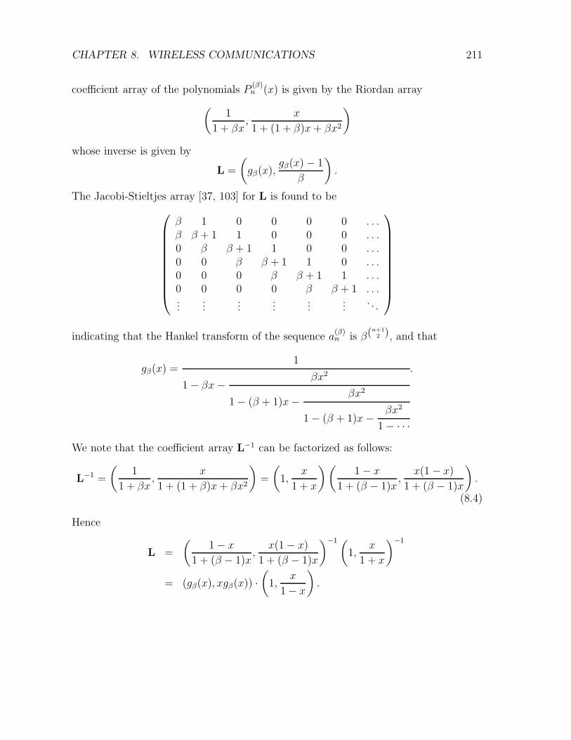
CHAPTER 8. WIRELESS COMMUNICATIONS 211
coefficient array of the polynomials P(β)n (x) is given by the Riordan array
(
1
1 + βx,
x
1 + (1 + β)x + βx2
)
whose inverse is given by
L =
(
gβ(x),gβ(x) − 1
β
)
.
The Jacobi-Stieltjes array [37, 103] for L is found to be
β 1 0 0 0 0 . . .β β + 1 1 0 0 0 . . .0 β β + 1 1 0 0 . . .0 0 β β + 1 1 0 . . .0 0 0 β β + 1 1 . . .0 0 0 0 β β + 1 . . ....
......
......
.... . .
indicating that the Hankel transform of the sequence a(β)n is β(n+1
2 ), and that
gβ(x) =1
1 − βx− βx2
1 − (β + 1)x− βx2
1 − (β + 1)x− βx2
1 − · · ·
.
We note that the coefficient array L−1 can be factorized as follows:
L−1 =
(
1
1 + βx,
x
1 + (1 + β)x + βx2
)
=
(
1,x
1 + x
)(
1 − x
1 + (β − 1)x,
x(1 − x)
1 + (β − 1)x
)
.
(8.4)
Hence
L =
(
1 − x
1 + (β − 1)x,
x(1 − x)
1 + (β − 1)x
)−1(
1,x
1 + x
)−1
= (gβ(x), xgβ(x)) ·(
1,x
1 − x
)
.

CHAPTER 8. WIRELESS COMMUNICATIONS 212
The general term of the matrix(
1 − x
1 + (β − 1)x,
x(1 − x)
1 + (β − 1)x
)−1
= (gβ(x), xgβ(x))
is given by
k + 1
n + 1
n−k∑
j=0
(
n + 1
k + j + 1
)(
n + j
j
)
(β−1)n−k−j =n−k∑
j=0
k + 1
k + j + 1
(
n
k + j
)(
n + j
j
)
(β−1)n−k−j.
For instance, when β = 1, which is the case of the matrix (1 − x, x(1 − x))−1, we getthe expression
k + 1
n + 1
(
2n− k
n− k
)
for the general term. Now the general term of the matrix(
1, 11−x
)
is given by
(
n− 1
k − 1
)
+ 0n(−1)k.
Hence the general term of L is given by
n∑
j=0
n−j∑
i=0
j + 1
i + j + 1
(
n
i + j
)(
n + i
i
)
(β − 1)n−j−i(
(
j − 1
k − 1
)
+ 0j(−1)k). (8.5)
It is interesting to note that
L−1 =
(
1 + x
(1 + x)(1 + βx),
x
(1 + x)(1 + βx)
)
. (8.6)
We can use the factorization in eq. (8.4) to express the orthogonal polynomials P(β)n (x)
in terms of the Chebyshev polynomials of the second kind Un(x). Thus we recognizethat the Riordan array
(
1
1 + (β + 1)x + βx2,
x
1 + (1 + β)x + βx2
)
is the coefficient array of the modified Chebyshev polynomials of the second kindβ
n2Un(x−(β+1)
2√β
). Hence by the factorization in eq. (8.4) we obtain
P (β)n (x) = β
n2Un(
x− (β + 1)
2√β
) + βn−12 Un−1(
x− (β + 1)
2√β
). (8.7)

CHAPTER 8. WIRELESS COMMUNICATIONS 213
8.3 The R Transform
Along with the Stieltjes transform, another transform which has been shown to simplifycalculations in random matrix theory is the R transform. The R transform, in relationto the Stieltjes transform can be defined as follows
Definition 8.3.1. Given P (x), some probability distribution, with Stieltjes transform
G(s) =
∫
dP (x)
x− s
then the R transform of P (X) is
R(w) = G−1(−w) − 1
w
Example. The R transform of the Marcenko and Pastur law is
R(w) =1
1 − αw
Looking at an example [95], let P (x) be a probability distribution with
GX−1(s) =
∫
dPX(x)1x− s
existing for some complex s with Im(s) > 0
GX−1
(
1
s
)
= −s(1 + sGX(s))
Let s = G−1X (−w), so we find
GX−1
(
1
G−1X (−w)
)
= −G−1X (−w)(1 − wG−1
X (−w))
(
1
G−1X (−w)
)
= G−1X−1
(
−G−1X (−w)(1 − wG−1
X (−w)))
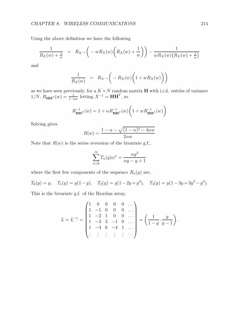
CHAPTER 8. WIRELESS COMMUNICATIONS 214
Using the above definition we have the following
1
RX(w) + 1w
= RX−1
(
− wRX(w)
(
RX(w) +1
w
))
− 1
wRX(w)(
RX(w) + 1w
)
and
1
RX(w)= RX−1
(
− RX(w)
(
1 + wRX(w)
))
as we have seen previously, for a K×N random matrix H with i.i.d. entries of variance1/N , R
HHT (w) = 1
1−αwletting X−1 = HHT , so
R−1HH
T (w) = 1 + αR−1HH
T (w)
(
1 + wR−1HH
T (w)
)
Solving gives
R(w) =1 − α−
√
(1 − α)2 − 4αw
2αw
Note that R(w) is the series reversion of the bivariate g.f.,
∞∑
n=0
Tn(y)αn =αy2
αy − y + 1
where the first few components of the sequence Rn(y) are,
T0(y) = y, T1(y) = y(1− y), T2(y) = y(1−2y+ y2), T3(y) = y(1−3y+ 3y2− y3).
This is the bivariate g.f. of the Riordan array,
L = L−1 =
1 0 0 0 0 . . .1 −1 0 0 0 . . .1 −2 1 0 0 . . .1 −3 3 −1 0 . . .1 −4 6 −4 1 . . ....
......
......
. . .
=
(
1
1 − y,
y
y − 1
)
.

Chapter 9
The Euler-Seidel matrix
The Euler-Seidel matrix [39, 40, 41, 49, 91] of a sequence (an)n≥0, which we will de-note by E = Ea, is defined to be the rectangular array (an,k)n,k≥0 determined by therecurrence a0,k = ak (k ≥ 0) and
an,k = an−1,k + an−1,k+1 (n ≥ 1, k ≥ 0). (9.1)
The sequence (a0,k), the first row of the matrix, is usually called the initial sequence,while the sequence (an,0), first column of the matrix, is called the final sequence. Theyare related by the binomial transform (or Euler transform, after Euler, who first provedthis [53]). We recall that the binomial transform of a sequence an has general termbn =
∑nk=0
(
nk
)
ak. Thus the first row and column of the matrix are determined fromeq. (9.1) as follows:
an,0 =n∑
k=0
(
n
k
)
a0,k, (9.2)
a0,n =
n∑
k=0
(
n
k
)
(−1)n−kak,0. (9.3)
In general, we have
an,k =n∑
i=0
(
n
i
)
a0,i+k =n∑
i=0
(
n
i
)
ai+k. (9.4)
215

CHAPTER 9. THE EULER-SEIDEL MATRIX 216
Example. We take a0,n = an = Cn = 1n+1
(
2nn
)
, the Catalan numbers. Thus the initial
sequence, or first row, is the Catalan numbers, while the final sequence, or first column,
will be the binomial transform of the Catalan numbers. We obtain the following matrix:
1 1 2 5 14 42 . . .
2 3 7 19 56 174 . . .
5 10 26 75 230 735 . . .
15 36 101 305 965 3155 . . .
51 137 406 1270 4120 13726 . . .
188 543 1676 5390 17846 60398 . . ....
......
......
.... . .
.
We now remark that the Catalan numbers Cn, (A000108) have the following moment
representation:
Cn =1
2π
∫ 4
0
xn
√
x(4 − x)
xdx. (9.5)
Many of the sequences we will discuss have a moment representation of the form
an =
∫
R
xndµa
for a suitable measure dµa.
Example. The aerated Catalan numbers. We have seen (see eq. (9.5)) that the
Catalan numbers are a moment sequence. Similarly, the aerated Catalan numbers
1, 0, 1, 0, 2, 0, 5, 0, 14, . . .
can by represented by
Cn2
1 + (−1)n
2=
1
2π
∫ 2
−2
xn√
4 − x2 dx.

CHAPTER 9. THE EULER-SEIDEL MATRIX 217
Example. The factorial numbers n!.
We have the well-known integral representation of n!, (A000142)
n! =
∫ ∞
0
xne−x dx.
Example. The aerated double factorials.
We recall that the double factorials (A001147) are given by
(2n− 1)!! =
n∏
k=1
(2k − 1) =(2n)!
n! 2n.
The aerated double factorials, which begin
1, 0, 3, 0, 5, 0, 15, 0, 105, 0, 945, . . .
have integral representation1√2π
∫ ∞
−∞xn e−
x2
2 dx.
The aerated double factorial numbers have e.g.f. ex2
2 .
9.1 The Euler-Seidel matrix and Hankel matrix for
moment sequences
We recall that for a sequence (an)n≥0, its Hankel matrix is the matrix H = Ha withgeneral term an+k. Note that if an has o.g.f. A(x) then the bivariate g.f. of Ha is givenby
xA(x) − yA(y)
x− y.
If an has an e.g.f. G(x), then the n-th row (and n-th column) of Ha has e.g.f. given by
dn
dxnG(x).

CHAPTER 9. THE EULER-SEIDEL MATRIX 218
Example. We have seen that the aerated double factorial numbers have e.g.f. ex2
2 .
Thus the n-th row of the Hankel matrix associated to them has e.g.f.
dn
dxne
x2
2 = ex2
2
⌊n2⌋
∑
k=0
(
n
2
)
(2k − 1)!!xn−2k.
Note that if
an =
∫
xndµa
then
an+k =
∫
xn+kdµa =
∫
xnxkdµa.
We recall that the binomial matrix is the matrix B with general term(
nk
)
. The binomialtransform of a sequence an is the sequence with general term
bn =
n∑
k=0
(
n
k
)
ak.
In this case, the sequence bn has o.g.f. given by
1
1 − xA
(
x
1 − x
)
.
The sequence (bn)n≥0 can be viewed as
B · (an)t.
Note that we have
bn =
n∑
k=0
(
n
k
)
ak
=n∑
k=0
(
n
k
)∫
xk dµa
=
∫ n∑
k=0
(
n
k
)
xk dµa
=
∫
(1 + x)n dµa.
In similar fashion, we have
an =
∫
(x− 1)n dµb.

CHAPTER 9. THE EULER-SEIDEL MATRIX 219
Proposition 9.1.1. We have
Ea = BHa. (9.6)
Proof. We have
BHa =
((
n
k
))
· (an+k) .
The result follows from eq. (9.4).
We now let
bn =
n∑
k=0
(
n
k
)
ak,
the binomial transform of an. We are interested in the product B−1Hb.
Example. Taking bn =∑n
k=0
(
nk
)
Ck (A0007317), the binomial transform of the Cata-
lan numbers Cn, we obtain
Hb =
1 2 5 15 51 188 . . .
2 5 15 51 188 731 . . .
5 15 51 188 731 2950 . . .
15 51 188 731 2950 12235 . . .
51 188 731 2950 12235 51822 . . .
188 731 2950 12235 51822 223191 . . ....
......
......
.... . .
.

CHAPTER 9. THE EULER-SEIDEL MATRIX 220
Multiplying by B−1, we obtain
B−1Hb =
1 2 5 15 51 188 . . .
1 3 10 36 137 543 . . .
2 7 26 101 406 1676 . . .
5 19 75 305 1270 5390 . . .
14 56 230 965 4120 17846 . . .
42 174 735 3155 13726 60398 . . ....
......
......
.... . .
,
which is the transpose of the Euler-Seidel matrix for Cn.
This result is general. In order to prove this, we will use the follow lemma.
Lemma 9.1.2.
xn(1 + x)k =k∑
i=0
(
k
i
)
xi+n =n∑
j=0
(−1)n−j
(
n
j
) j+k∑
i=0
(
j + k
i
)
xi. (9.7)
Proof. Since (1 + x)k =∑k
i=0
(
ki
)
xi by the binomial theorem, we immediately have
xn(1 + x)k = xn
k∑
i=0
(
k
i
)
xi =
k∑
i=0
(
k
i
)
xi+n.
But also, we have
n∑
j=0
(−1)n−j
(
n
j
) j+k∑
i=0
(
j + k
i
)
xi =
n∑
j=0
(−1)n−j
(
n
j
)
(1 + x)j+k
= (1 + x)kn∑
j=0
(−1)n−j
(
n
j
)
(1 + x)j
= (1 + x)kxn.

CHAPTER 9. THE EULER-SEIDEL MATRIX 221
Proposition 9.1.3. The Euler-Seidel matrix of the sequence (an)n≥0 is equal to the
transpose of the matrix given by B−1Hb, where Hb is the Hankel matrix of the binomial
transform
bn =n∑
k=0
(
n
k
)
ak
of the initial sequence an. That is,
Eta = B−1Hb. (9.8)
Proof. The general element of
B−1H =
(
(−1)n−k
(
n
k
))
· (bn+k)
is given byn∑
j=0
(−1)n−j
(
n
j
)
bj+k.
Now
n∑
j=0
(−1)n−j
(
n
j
)
bj+k =n∑
j=0
(−1)n−j
(
n
j
) j+k∑
i=0
(
j + k
i
)
ai.
Proposition 9.1.4.
n∑
j=0
(−1)n−j
(
n
j
) j+k∑
i=0
(
j + k
i
)
ai =
k∑
i=0
(
k
i
)
ai+n. (9.9)
Proof. Expanding 9.9, if k ≤ n − 2 we have (If k > n − 2, the middle term below
disappears)
n∑
j=0
(−1)n−j
(
n
j
)( k∑
i=0
(
j + k
i
)
ai +n−1∑
i=k+1
(
j + k
i
)
ai +n+k∑
i=n
(
j + k
i
)
ai
)
.

CHAPTER 9. THE EULER-SEIDEL MATRIX 222
Now, we endeavor to prove 9.9, by showing
n∑
j=0
(−1)n−j
(
n
j
) k∑
i=0
(
j + k
i
)
ai = 0 (9.10)
n∑
j=0
(−1)n−j
(
n
j
) n−1∑
i=k+1
(
j + k
i
)
ai = 0 (9.11)
n∑
j=0
(−1)n−j
(
n
j
) n+k∑
i=n
(
j + k
i
)
ai =
k∑
i=0
(
k
i
)
ai+n (9.12)
By a change of summation eq. (9.10) becomes
k∑
i=0
n∑
j=0
(−1)n−j
(
n
j
)(
j + k
i
)
ai =k∑
i=0
n∑
j=0
(−1)j(
n
n− j
)(
n− j + k
i
)
ai
=k∑
i=0
n∑
j=0
(−1)j(
n
j
)(
n− j + k
i
)
ai.
Using Vandermonde’s identity and a further change of summation we have
k∑
i=0
n∑
j=0
(−1)j(
n
j
)(
n− j + k
i
)
ai =k∑
i=0
n∑
j=0
(−1)j(
n
j
) i∑
r=0
(
n− j
r
)(
k
i− r
)
ai
=k∑
i=0
i∑
r=0
(
k
i− r
)
ai
n∑
j=0
(−1)j(
n
j
)(
n− j
r
)
=k∑
i=0
i∑
r=0
(
k
i− r
)
ai
n∑
j=0
(−1)j(
n
n− j
)(
n− j
r
)
.

CHAPTER 9. THE EULER-SEIDEL MATRIX 223
Now, by the cross product of binomial coefficients we have
=
k∑
i=0
i∑
r=0
(
k
i− r
)
ai
n∑
j=0
(−1)j(
n
n− j
)(
n− j
r
)
=
k∑
i=0
i∑
r=0
(
k
i− r
)
ai
n∑
j=0
(−1)j(
n
r
)(
n− r
n− j − r
)
=
k∑
i=0
i∑
r=0
(
k
i− r
)(
n
r
)
ai
n∑
j=0
(−1)j(
n− r
j
)
=
k∑
i=0
i∑
r=0
(
k
i− r
)(
n
r
)
ai
n−r∑
j=0
(−1)j(
n− r
j
)
.
Now as∑n−r
j=0 (−1)j(
n−rj
)
= 0, eq. (9.10) is satisfied. Now, with a change of summation
eq. (9.11) becomes
n∑
j=0
(−1)n−j
(
n
j
) n−1∑
i=k+1
(
j + k
i
)
ai =
n∑
j=0
(−1)n−j
(
n
j
) n−k−2∑
i=0
(
j + k
i + k + 1
)
ai+k+1
=
n−k−2∑
i=0
n∑
j=0
(−1)n−j
(
n
j
)(
k + j
k + i + 1
)
ai+k+1.
Expanding using Vandermonde’s identity and a further change of summation gives
=n−k−2∑
i=0
n∑
j=0
(−1)n−j
(
n
j
) k+i+1∑
r=0
(
k
r
)(
j
k + i + 1 − r
)
ak+i+1
=n−k−2∑
i=0
k+i+1∑
r=0
(
k
r
) n∑
j=0
(−1)n−j
(
n
j
)(
j
k + i + 1 − r
)
ak+i+1
=n−k−2∑
i=0
ak+i+1
k+i+1∑
r=0
(
k
r
) n∑
j=0
(−1)n−j
(
n
j
)(
j
k + i + 1 − r
)
.
Now, by the cross product of binomial coefficients we have
=
n−k−2∑
i=0
ak+i+1
k+i+1∑
r=0
(
k
r
) n∑
j=0
(−1)n−j
(
n
k + i + 1 − r
)(
n− (k + i + 1 − r)
j − (k + i + 1 − r)
)
=
n−k−2∑
i=0
ak+i+1
k+i+1∑
r=0
(
k
r
)(
n
k + i + 1 − r
) n∑
j=0
(−1)n−j
(
n− (k + i + 1 − r)
n− j
)
.

CHAPTER 9. THE EULER-SEIDEL MATRIX 224
Now r ≤ i so we have
n∑
j=0
(−1)n−j
(
n− (k + i + 1 − r)
n− j
)
=k+i+1−r∑
j=0
(−1)n−j
(
n− (k + i + 1 − r)
n− j
)
= 0,
so eq. (9.11) is satisfied. Lastly, eq. (9.12) with a summation change becomes
n∑
j=0
(−1)n−j
(
n
j
) k∑
i=0
(
j + k
i + n
)
ai+n =
k∑
i=0
n∑
j=0
(−1)n−j
(
n
j
)(
j + k
i + n
)
ai+n.
Expanding with Vandermonde’s identity and a further change of summation gives
=
k∑
i=0
n∑
j=0
(−1)n−j
(
n
j
) i+n∑
r=0
(
j
r
)(
k
i + n− r
)
ai+n
=
k∑
i=0
i+n∑
r=0
(
k
i + n− r
)
ai+n
n∑
j=0
(−1)n−j
(
n
j
)(
j
r
)
.
=
k∑
i=0
i+n∑
r=0
(
k
i + n− r
)
ai+n
n∑
j=0
(−1)n−j
(
n
r
)(
n− r
j − r
)
.
Nown∑
j=0
(−1)n−j
(
n− r
n− j
)
=
0 if 0 ≤ r < n
1 if r = n
sok∑
i=0
i+n∑
r=0
(
k
i + n− r
)
ai+n
n∑
j=0
(−1)n−j
(
n
r
)(
n− r
j − r
)
=
k∑
i=0
(
k
i
)
ai+n.
Eq. (9.12) is satisfied.
The result follows from eq. (9.4).
Corollary 9.1.5. The nth row of Ea, for an e.g.f. A(x) is
exdn
dx(A(x)) .

CHAPTER 9. THE EULER-SEIDEL MATRIX 225
Proof. Using the fact that Ea = BHa where Ha is the Hankel matrix of the first column
of the Euler Seidel matrix Ea, for an e.g.f. A(x), the columns of the Euler Seidel matrix
have the form
[ex, x]d
dx(A(x))
and using the fundamental theorem of Riordan arrays the nth column have the g.f.
exdn
dx(A(x)) .
Example. The aerated double factorial numbers which have the e.g.f. ex2
2 have first
few rows of Ea,
1 0 0 0 0 . . .
1 1 0 0 0 . . .
1 2 1 0 0 . . .
1 3 3 1 0 . . .
1 4 6 4 1 . . .
1 5 10 10 5 . . ....
......
......
. . .
1 0 1 0 3 . . .
0 1 0 3 0 . . .
1 0 3 0 15 . . .
0 3 0 15 0 . . .
3 0 15 0 105 . . .
0 15 0 105 0 . . ....
......
......
. . .
=
1 0 1 0 3 . . .
1 1 1 3 3 . . .
2 2 4 6 18 . . .
4 6 10 24 48 . . .
10 16 34 72 198 . . .
26 50 106 270 678 . . ....
......
......
. . .
So the nth column of Ea is
[ex, x]dn
dx
(
ex2
2
)
= exdn
dx
(
ex2
2
)
.
The nth derivative of dn
dx
(
ex2
2
)
as we have seen in proposition 9.13 can be expressed as
ex2
2
⌊n2⌋
∑
r=0
(
n
n− 2r
)
(2r − 1)!!xn−2r.

CHAPTER 9. THE EULER-SEIDEL MATRIX 226
Thus the columns of Ea have the form
exdn
dx
(
ex2
2
)
= exex2
2
⌊n2⌋
∑
r=0
(
n
n− 2r
)
(2r − 1)!!xn−2r
= ex2
2+x
⌊n2⌋
∑
r=0
(
n
n− 2r
)
(2r − 1)!!xn−2r.
Since ex2
2+x is the e.g.f. of the Young Tableaux numbers, A000085 we have
exdn
dx
(
ex2
2
)
= ex2
2+x
⌊n2⌋
∑
r=0
(
n
n− 2r
)
(2r − 1)!!xn−2r
=∞∑
n=0
Ynxn
n
⌊n2⌋
∑
r=0
(
n
n− 2r
)
(2r − 1)!!xn−2r.
We generalize this result to the e.g.f. eαx2. As the nth row of a Hankel matrix generated
from the e.g.f. eαx2
is the nth derivative of eαx2
we introduce the following proposition.
Proposition 9.1.6.
dn+1
dxn+1
(
eαx2)
=d
dx
eαx2
⌊n2⌋
∑
r=0
(2α)n−r(
nn−2r
)
(2r)!
r!2rxn−2r
= eαx2
⌊n+12
⌋∑
r=0
(2α)n+1−r(
n+1n+1−2r
)
(2r)!
r!2rxn+1−2r.
(9.13)

CHAPTER 9. THE EULER-SEIDEL MATRIX 227
Proof. Firstly, let us illustrate the expansion of the e.g.f. for the first few values of n
d
dx
(
eαx2)
= eαx2
(2αx)
= eαx2
(
2α
(
1
1
)
x
)
d2
dx
(
eαx2)
= eαx2
(4α2x2 + 2α)
= eαx2
(
22α2
(
2
2
)
x2 + 2α
(
2
0
))
d3
dx
(
eαx2)
= eαx2
(8α3x3 + 12α2x)
= eαx2
(
23α3
(
3
3
)
x3 + 22α2
(
3
1
)
x
)
d4
dx
(
eαx2)
= eαx2
(16α4x4 + 48α3x2 + 12α2)
= eαx2
(
24α4
(
4
4
)
x4 + 23α3
(
4
2
)
x2 + 22α23
(
4
0
))
d5
dx
(
eαx2)
= eαx2
(eαx2
(32α5x5 + 160α4x3 + 120α3x)
= eαx2
(
25α5
(
5
5
)
x5 + 24α4
(
5
3
)
x3 + 23α33
(
5
1
)
x
)
.
Expanding
d
dx
eαx2
⌊n2⌋
∑
r=0
(2α)n−r(
nn−2r
)
(2r)!
r!2rxn−2r
we have
eαx2
xn−1(2α)nn!
{ ⌊n2⌋
∑
r=0
α−r+12−2r+1x−2r+2
r!(n− 2r)!−
⌊n2⌋
∑
r=0
α−r2−2r+1x−2r
(r − 1)!(n− 2r)!+
⌊n2⌋
∑
r=0
nα−r2−2rx−2r
r!(n− 2r)!
}
,
and gathering similar terms we have
emx2
xn−1(2α)nn!
{
2αx2
n!+
⌊n2⌋
∑
r=1
α−r+12−2r+1x−2r+2(n + 1)
r!(n− 2r + 1)!+
2−2⌊n2⌋α⌊n
2⌋+nx⌊n
2⌋+n−1n!
⌊n2⌋!(n− 2(⌊n
2⌋) + 1)!
}

CHAPTER 9. THE EULER-SEIDEL MATRIX 228
which summarizes to
= eαx2
⌊n+12
⌋∑
r=0
(2α)n+1−r(
n+1n+1−2r
)
(2r)!
r!2rxn+1−2r.
We are interested in characterising the main diagonal of the Euler-Seidel matrix of an,which by the above is the same as the main diagonal of B−1Hb, where H is the Hankelmatrix of bn, the binomial transform of an.
Note that the diagonal is given by
an,n =
n∑
i=0
(
n
i
)
an+i.
Example. We have seen that the diagonal of the Euler-Seidel matrix for the Catalan
numbers Cn begins
1, 3, 26, 305, 4120, 60398, 934064, . . .
By the above, the general term of this sequence is
dn =n∑
i=0
(
n
i
)
Cn+i.
Now consider the moment representation of the Catalan numbers given by
Cn =
∫
xndµ =1
2π
∫ 4
0
xn
√
x(4 − x)
xdx.
We claim that
dn =
∫
(x(1 + x))ndµ =1
2π
∫ 4
0
(x(1 + x))n√
x(4 − x)
xdx.
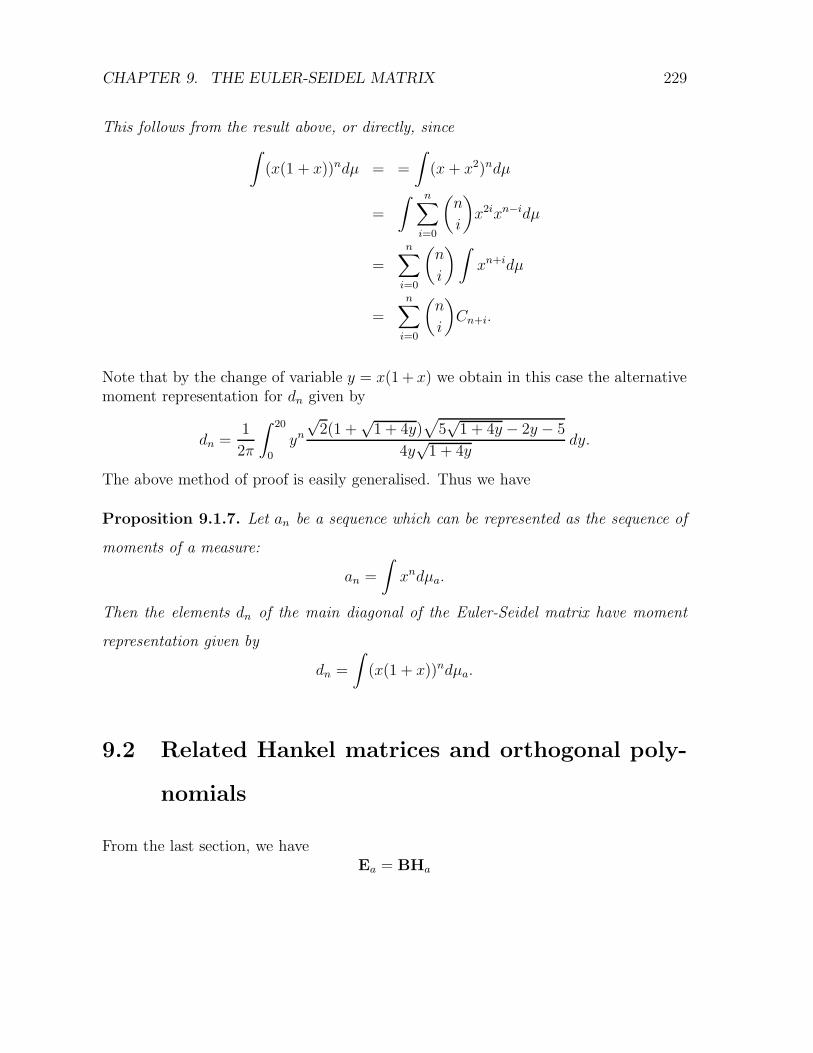
CHAPTER 9. THE EULER-SEIDEL MATRIX 229
This follows from the result above, or directly, since∫
(x(1 + x))ndµ = =
∫
(x + x2)ndµ
=
∫ n∑
i=0
(
n
i
)
x2ixn−idµ
=
n∑
i=0
(
n
i
)∫
xn+idµ
=n∑
i=0
(
n
i
)
Cn+i.
Note that by the change of variable y = x(1 + x) we obtain in this case the alternativemoment representation for dn given by
dn =1
2π
∫ 20
0
yn√
2(1 +√
1 + 4y)√
5√
1 + 4y − 2y − 5
4y√
1 + 4ydy.
The above method of proof is easily generalised. Thus we have
Proposition 9.1.7. Let an be a sequence which can be represented as the sequence of
moments of a measure:
an =
∫
xndµa.
Then the elements dn of the main diagonal of the Euler-Seidel matrix have moment
representation given by
dn =
∫
(x(1 + x))ndµa.
9.2 Related Hankel matrices and orthogonal poly-
nomials
From the last section, we haveEa = BHa

CHAPTER 9. THE EULER-SEIDEL MATRIX 230
andEt
a = B−1Hb
where bn is the binomial transform of an. The second equation shows us that
Ea = (B−1Hb)t
= Htb(B
−1)t
= Hb(Bt)−1,
since Hb is symmetric. Thus we obtain
BHa = Hb(Bt)−1,
which implies thatHb = BHaB
t. (9.14)
Since det(B) = 1, we deduce once again that the Hankel transform of bn is equal to thatof an. We can also use this result to relate the LDU decomposition of Hb [103, 164]to that of Ha. Thus we have
Hb = BHaBt
= B · LaDaLta · Bt
= (BLa)Da(BLa)t.
One consequence of this is that the coefficient triangle of the polynomials orthogonalwith respect to dµb is given by
L−1a B−1,
where L−1a is the coefficient array of the polynomials orthogonal with respect to dµa.
Example. We take the example of the Catalan numbers an = Cn and their binomial
transform bn =∑n
k=0Ck. It is well known that the Hankel transform of Cn is the all
1’s sequence, which implies that Da is the identity matrix. Thus in this case,
Ha = LaLat
where
La = LCn= (c(x), xc(x)2) (A039599)

CHAPTER 9. THE EULER-SEIDEL MATRIX 231
with
L−1a =
(
1
1 + x,
x
(1 + x)2
)
(A129818)
with general term (−1)n−k(
n+k2k
)
, where we have used the notation of Riordan arrays.
The polynomials
Pn(x) =
n∑
k=0
(−1)n−k
(
n + k
2k
)
xk
are thus a family of polynomials orthogonal on [0, 4] with respect to the density function
12π
√x(4−x)
x[157]. It is known that the bivariate g.f. of the inverse of the n-th principal
minor of Ha is given by the Christoffel-Darboux quotient
Pn+1(x)Pn(y) − Pn+1(y)Pn(x)
x− y.
We deduce that the orthogonal polynomials defined by bn have coefficient matrix
L−1b = L−1
a B−1
=
(
1
1 + x,
x
(1 + x)2
)
·(
1
1 + x,
x
1 + x
)
=
(
1 + x
1 + 3x + x2,
x
1 + 3x + x2
)
.
It turns out that these polynomials Qn(x) are given simply by
Qn(x) = Pn(x− 1).
Thus H−1b has n-th principal minor generated by
Qn+1(x)Qn(y) −Qn+1(y)Qn(x)
x− y.
In similar manner, we can deduce that the Euler-Seidel matrix Ea = ECnis such that
the n-th principal minor of E−1a is generated by
Pn+1(x)Pn(y − 1) − Pn+1(y − 1)Pn(x)
x− y=
Pn+1(x)Qn(y) −Qn+1(y)Pn(x)
x− y.

CHAPTER 9. THE EULER-SEIDEL MATRIX 232
Example. For the aerated double factorials, we have
Ha = LaDaLta
where
La = [ex2
2 , x], Da = diag(n!).
The associated orthogonal polynomials (which are scaled Hermite polynomials) have
coefficient matrix
L−1a = [e−
x2
2 , x],
and we have
Pn(x) =
⌊n2⌋
∑
k=0
(
n
2k
)
(2k − 1)!!(−1)kxn−2k,
or equivalently,
Pn(x) =
n∑
k=0
Bessel∗(
n + k
2, k
)
(−1)n−k2
1 + (−1)n−k
2xk,
where
Bessel∗(n, k) =(2n− k)!
k!(n− k)!2n−k=
(
n + k
2k
)
(2k − 1)!!,
(see [9]). With
Qn(x) = Pn(x− 1)
we again have that the Euler-Seidel matrix Ea is such the n-th principal minor of E−1a
is generated by
Pn+1(x)Pn(y − 1) − Pn+1(y − 1)Pn(x)
x− y=
Pn+1(x)Qn(y) −Qn+1(y)Pn(x)
x− y.

Chapter 10
Conclusions and future directions
Riordan arrays and orthogonal polynomials have been areas of particular interestthroughout this study. In Chapter 3 we focused on algebraic structures in Hankelmatrices and Hankel-plus-Toeplitz matrices relating to classical orthogonal polynomi-als, in particular the Chebyshev polynomials. Future work involves extending ourresearch to establish links between such algebraic structures and other classical andsemi-classical orthogonal polynomials.
Continuing our emphasis on links between Riordan arrays and orthogonal polynomials,we have studied elements of an important property of OPS’s, the three-term recurrencerelation. Specifically, we have studied the coefficients of the recurrence relations, relatedpaths, and continued fraction expansions, all in the context of associated Riordanarrays. In future work we can extend this focus on the coefficients to study howthe existence of recursive relations between these coefficients can be linked to thecorresponding Riordan arrays. Another area of possible exploration is the link betweenthe “ladder operator” [25] approach and the Riordan array approach.
Riordan arrays and lattice paths have also been of interest in this thesis. We have beenespecially interested in lattice paths corresponding to Riordan arrays that are related toorthogonal polynomials and how the structure of these paths relate to general Riordanarrays. In [14] we have shown that Riordan arrays of the form
(
1 − λx− µx2
1 + rx + sx2,
x
1 + rx + sx2
)
233

CHAPTER 10. CONCLUSIONS AND FUTURE DIRECTIONS 234
Figure 10.1: A Dyck path of weight s3(µ + s)rs(µ + s)
are the coefficient arrays of orthogonal polynomials. The related Stieltjes matrix hasthe form
λ + r 1 0 0 . . .µ + s r 1 0 . . .
0 s r 1 . . .0 0 s r . . ....
......
. . .
.
The corresponding Motzkin paths have weighting λ + r for level steps on the x axis,µ+ s for S-E steps returning to the x axis, and all other S-E steps of weight s and levelsteps of weight r. Fig. (10.1) shows an example of one such path.
We have shown that the Hankel matrix generated from the sequence formed from thefirst column of the inverse of the Riordan array above, can de decomposed in such away to yield a Riordan array with related non-tridiagonal Stieljtes matrix of the form
λ + r 1 0 0 . . .µ + s r − 1 1 0 . . .µ + s s r − 1 1 . . .µ + s s s r − 1 . . .
......
.... . .
.

CHAPTER 10. CONCLUSIONS AND FUTURE DIRECTIONS 235
We have shown that this matrix relates to Lukasiewicz paths of weighting λ + r forlevel steps on the x axis, µ + s for S-E Lukasiewicz steps returning to the x axis, andall other S-E Lukasiewicz steps of weight s and level steps of weight r − 1.
We exhibited a bijection between these two types of Motkzin and Lukasiewicz paths.Below we show the associated weights for both Lukasiewicz and Motzkin paths for apath of length 4.
(µ + s)2 = (µ + s)2 s(µ + s) = s(µ + s)
(µ + s)(λ + r)2 = (µ + s)(λ + r)2 (λ + r)(µ + s)(λ + r) = (λ + r)(µ + s)(λ + r)
(λ + r)2(µ + s) = (λ + r)2(µ + s) (λ + r)4 = (λ + r)4
r2(µ + s) = (r − 1)2(µ + s) + (r − 1)(µ + s) + (r − 1)(µ + s) + (µ + s)
r(µ + s)(λ + r) = (r − 1)(µ + s)(λ + r) + (µ + s)(λ + r)
(λ + r)(µ + s)(r) = (λ + r)(r − 1)(µ + s) + (λ + r)(µ + s)
Riordan arrays relating to the paths above are ordinary Riordan arrays. Some ofthe above work extended to exponential Riordan arrays. Future work could involveestablishing bijections between Motkin and Lukasiewicz paths relating to exponentialRiordan arrays.
Recent work carried out by Dan Drake [45] shows bijections between weighted Dyckpaths and Schroder paths. Drake also studied bijections between matchings and certainpaths. In a similar manner, we can explore the possibilities of extending our combi-

CHAPTER 10. CONCLUSIONS AND FUTURE DIRECTIONS 236
natorial interpretations to matchings and to study bijections arising between thesematchings and Lukasiewicz paths. We may also seek to extend our work on Riordanarrays to other combinatorial interpretations, noting that Viennot and Flajolet stud-ied many forms of combinatorial interpretations relating to orthogonal polynomials.Recent work in this field has been carried out by Louis Shapiro who has studied treestructures relating to Riordan arrays [120].
As with the bijections proved in this thesis, we can continue to explore similar bijec-tions in the area of restricted paths. Such paths have been shown to model polymerabsorbtion [108].
Using continued fractions expansions, expressions have been derived for q-orthogonalpolynomials related to restricted Dyck paths. We can explore the possibility, using thelinks we have established between Motzkin paths relating to orthogonal polynomialsand corresponding Lukasiewicz paths, of extending this to q-orthogonal polynomials.
Finally, we distinguished between three different “Narayana triangles” and their as-sociated “Narayana polynomials”and applied these polynomials in the area of MIMO(multiple input, multiple output) wireless communication. We expressed the channelcapacity for a MIMO channel using one of the Narayana polynomials. This gave us thefollowing result:
CMIMO =β
ln 2
N∑
k=0
pk(σ2T )k
[xk+1]Revx
[
x(1 − x)
1 − (1 − β)x
]
. (10.1)
In calculating the channel capacity, the Stieltjes transform was used. Extending onthis work, we looked at the use of other transforms, such as the R [95] transform toestablish similar results. We hope to develop on this work.

Appendix A
Appendix
A.1 Published articles
A.1.1 Journal of Integer Sequences, Vol. 12 (2009), Article
09.5.3
Notes on a Family of Riordan Arrays and Associated Integer Hankel Transforms
Abstract: We examine a set of special Riordan arrays, their inverses and associatedHankel transforms.
P. Barry and A. Hennessy, Notes on a Family of Riordan Arrays and Associated IntegerHankel transforms, J. Integer Seq. ON. ISSN 1530-7638, Vol. 12, (2009), Article 09.05.3.
237

APPENDIX A. APPENDIX 238
A.1.2 Journal of Integer Sequences, Vol. 13 (2010), Article
10.9.4
Meixner − Type Results for Riordan Arrays and Associated Integer Sequence
Abstract: We determine which (ordinary) Riordan arrays are the coefficient arrays ofa family of orthogonal polynomials. In so doing, we are led to introduce a family ofpolynomials, which includes the Boubaker polynomials, and a scaled version of theChebyshev polynomials, using the techniques of Riordan arrays. We classify thesepolynomials in terms of the Chebyshev polynomials of the first and second kinds. Wealso examine the Hankel transforms of sequences associated with the inverse of thepolynomial coefficient arrays, including the associated moment sequences.
P. Barry and A. Hennessy, Meixner-type results for Riordan arrays and associatedinteger sequences, J. Integer Seq. ON. ISSN 1530-7638, Vol. 13, (2010), Article 10.9.4.

APPENDIX A. APPENDIX 239
A.1.3 Journal of Integer Sequences, Vol. 13 (2010), Article
10.8.2
The Euler − Seidel Matrix, Hankel Matrices and Moment Sequences
Abstract: We study the Euler-Seidel matrix of certain integer sequences, using thebinomial transform and Hankel matrices. For moment sequences, we give an integralrepresentation of the Euler-Seidel matrix. Links are drawn to Riordan arrays, orthog-onal polynomials, and Christoffel-Darboux expressions.
P. Barry and A. Hennessy, The Euler-Seidel Matrix, Hankel Matrices and MomentSequences, J. Integer Seq. ON. ISSN 1530-7638, Vol. 13, (2010), Article 10.8.2.

APPENDIX A. APPENDIX 240
A.1.4 Journal of Integer Sequences, Vol. 14 (2011), Article
11.3.8
A Note on Narayana Triangles and Related Polynomials, Riordan Arrays,and MIMO Capacity Calculations
Abstract: We study the Narayana triangles and related families of polynomials. Welink this study to Riordan arrays and Hankel transforms arising from a special case ofcapacity calculation related to MIMO communication systems. A link is establishedbetween a channel capacity calculation and a series reversion.
P. Barry, A Hennessy, A note on Narayana triangles and related polynomials, Riordanarrays, and MIMO capacity calculations, J. Integer Seq. ON. ISSN 1530-7638, Vol.14 (2011), Article 11.3.8.

APPENDIX A. APPENDIX 241
A.1.5 Journal of Integer Sequences, Vol. 14 (2011), Article
11.8.2
Generalized Stirling Numbers, Exponential Riordan Arrays, and OrthogonalPolynomials.
Abstract: We define a generalization of the Stirling numbers of the second kind, whichdepends on two parameters. The matrices of integers that result are exponential Ri-ordan arrays. We explore links to orthogonal polynomials by studying the productionmatrices of these Riordan arrays. Generalized Bell numbers are also defined, again de-pending on two parameters, and we determine the Hankel transform of these numbers.
A. Hennessy, P. Barry, Generalized Stirling Numbers, Exponential Riordan Arrays,and Orthogonal Polynomials, J. Integer Seq. ON. ISSN 1530-7638, Vol. 14 (2011),Article 11.8.2.

APPENDIX A. APPENDIX 242
A.2 Submitted articles
A.2.1 Cornell University Library, arXiv:1101.2605
Riordan arrays and the LDU decomposition of symmetric Toeplitz plus Hankelmatrices
(Submitted on 13 Jan 2011)
Abstract: We examine a result of Basor and Ehrhardt concerning Hankel and Toeplitzplus Hankel matrices, within the context of the Riordan group of lower-triangularmatrices. This allows us to determine the LDU decomposition of certain symmetricToeplitz plus Hankel matrices. We also determine the generating functions and Hankeltransforms of associated sequences.
P. Barry and A. Hennessy, Riordan arrays and the LDU decomposition of symmetricToeplitz-plus-Hankel matrices, published electronically at:http://arxiv.org/abs/1101.2605, 2011.

Bibliography
[1] T. W. Anderson, R. A. Fisher and Multivariate Analysis, Journal of StatisticalScience, Vol. 11, No. 1, (1996), pp. 20–34.
[2] T. W. Anderson, An Introduction to Multivariate Statistical Analysis, 3rd Edi-tion, ISBN: 978-0-471-36091-9, 2003.
[3] Z. D. Bai, Methodologies in spectral analysis of large dimensional random ma-trices, a review (with discussion) Statist. Sinica, Taipei. ISSN 1017-0405, Vol. 9,(1999), pp. 611–677.
[4] J. Baik and J. W. Silverstein, Eigenvalues of large sample covariance matrices ofspiked population models, Journal of Multivariate Analysis. ISSN 0047-259, Vol.97, No. 6, (2006), pp. 1382–1408.
[5] J. Baik, P. A. Deift, and K. Johansson. On the distribution of the length of thelongest increasing subsequence of random permutations, Journal of the Amer.Math. Soc., Providence, RI. ISSN 0894-0347, Vol. 12, Issue 4, (1999), pp. 1119–1178.
[6] P. Barry, Continued fractions and transformations of integer sequences, J. IntegerSeq., Waterloo, ON. ISSN 1530-7638, Vol. 12, (2009),Article 9.7.6.
[7] P. Barry, On a One-Parameter Family of Riordan Arrays and the Weight Distri-bution of MDS Codes, J. Integer Seq., Waterloo, ON. ISSN 1530-7638, Vol. 10,(2007), Article 07.9.8.
[8] P. Barry, On Integer-Sequence-Based Constructions of Generalized Pascal Tri-angles, J. Integer Seq., Waterloo, ON. ISSN 1530-7638, Vol. 9, (2006),Article 06.2.4.
243

BIBLIOGRAPHY 244
[9] P. Barry, On a family of generalized Pascal’s triangles defined by exponentialRiordan arrays, J. Integer Seq., Waterloo, ON. ISSN 1530-7638, Vol. 10, (2000),Article 07.3.5.
[10] P. Barry, The Restricted Toda Chain, Exponential Riordan Arrays, and Han-kel Transforms, J. Integer Seq., Waterloo, ON. ISSN 1530-7638, Vol. 13,(2010),Article 10.8.4.
[11] P. Barry, P. Rajkovic and M. Petkovic, The Hankel transforms based on the cen-tral coefficients of certain Pascal-like triangles, Integral Transforms and SpecialFunctions. An International Journal. Taylor & Francis, Abingdon. ISSN 1065-2469, Vol. 18, Issue 4 (2007), pp. 285–296.
[12] P. Barry, P. Rajkovic and M. Petkovic, An application of Sobolev orthogonalpolynomials to the computation of a special Hankel Determinant, in W. Gautschi,G. Rassias, M. Themistocles (Eds), Approximation and Computation, Springer,2010.
[13] P. Barry, A Hennessy, A note on Narayana triangles and related polynomials,Riordan arrays, and MIMO capacity calculations, J. Integer Seq. ON. ISSN 1530-7638, Vol. 14 (2011), Article 11.3.8.
[14] P. Barry and A. Hennessy, Meixner-type results for Riordan arrays and associ-ated integer sequences, J. Integer Seq. ON. ISSN 1530-7638, Vol. 13, (2010),Article 10.9.4.
[15] P. Barry and A. Hennessy, The Euler-Seidel Matrix, Hankel Matrices andMoment Sequences, J. Integer Seq. ON. ISSN 1530-7638, Vol. 13, (2010),Article 10.9.4.
[16] P. Barry and A. Hennessy, Notes on a Family of Riordan Arrays and AssociatedInteger Hankel transforms, J. Integer Seq. ON. ISSN 1530-7638, Vol. 13, (2010),Article 09.05.3.
[17] P. Barry and A. Hennessy, Riordan arrays and the LDU decomposi-tion of symmetric Toeplitz-plus-Hankel matrices, published electronically athttp://arxiv.org/abs/1101.2605, 2011.
[18] E. Basor and T. Ehrhardt, Some identities for determinants of structured matri-ces. Special issue on structured and infinite systems of linear equations, LinearAlgebra and its Applications. ISSN 0024-3795, Vol. 343/344, (2002), pp. 5–19.

BIBLIOGRAPHY 245
[19] C. Berg, Moment problems and orthogonal polynomials, Seriesof lectures, University of Copenhagen, available electronically athttp://www.math.ku.dk/kurser/2005-06/blok2/moment/intro.pdf, 2005.
[20] J. P. Bouchard and M. Potters, Theory of Financial Risk and Derivative Pricing,University Press, Cambridge, 2003.
[21] P. Branden, A. Claesson & E. Steingrımsson, Catalan continued frac-tions and increasing subsequences in permutations, available electronically athttp://www.cs.chalmers.se/ claesson/papers/kb13.ps, 2009.
[22] P. Branden, The generating function of two-stack sortable per-mutations by descents is real-rooted, published electronically athttp://arxiv.org/abs/math/0303149, 2003.
[23] F. Chapoton, Enumerative properties of Generalized Associahedra, Sem. Lothar.Combin. Vol. 51, 2004.
[24] W.Y.C. Chen, S.H.F. Yan and L.L.M. Yang, Identitiesfrom weighted 2-Motzkin paths, published electronically athttp://arxiv.org/pdf/math.CO/0410200.pdf, 2006.
[25] Y. Chen and M. R. Mckay, Perturbed Hankel determinants: Applications to theinformation theory of MIMO wireless communications, , published electronicallyat http://arxiv.org/abs/1007.0496, 2010.
[26] G. Cheon, H. Kim, L. W. Shapiro, The hitting time subgroup, L ukasiewiczpaths and Faber polynomials, European Journal of Combinatorics, Vol. 32, Issue1, 2011.
[27] T. S. Chihara, An Introduction to Orthogonal Polynomials, Gordon and Breach,New York, 1978.
[28] C. Coker, Enumerating a class of lattice paths, Discrete Mathematics. ElsevierSci. B. V., Amsterdam. ISSN 0012-365X, 271, (2003) pp. 13–28.
[29] J. B. Conroy, The Riemann Hypothesis, Notices of the American Institute ofMathematics, 2003.
[30] T. Conlon, H. J. Ruskin and M. Crane, Random matrix theory and fund offunds portfolio optimisation, Dublin City University, Physica A, Vol. 382, Issue2 (2007), pp. 565-576.

BIBLIOGRAPHY 246
[31] A. G. Constantine, Some noncentral distribution problems in multivariate analy-sis, Annals of Mathematical Statististics, Vol. 34, No. 4, (1963), pp. 1270–1285.
[32] C. Corsani, D. Merlini, R. Sprugnoli, Left-inversion of combinatorial sums, Dis-crete Mathematics. Elsevier Sci. B. V., Amsterdam. ISSN 0012-365X, Vol. 180(1998), pp. 107–122.
[33] A. Cvetkovic, P. Rajkovic and M. Ivkovic, Catalan Numbers, the Hankel Trans-form and Fibonacci Numbers, J. Integer Seq., Waterloo, ON. ISSN 1530-7638,Vol. 5, (2002), Article 02.1.3.
[34] R. Dawkins, River out of Eden, HarperCollins, Part of the Science Masters series,ASIN 0465069908, 1995.
[35] E. Deutch and L. Shapiro, Exponential Riordan Arrays, Lec-ture Notes, Nankai University, available electronically athttp://www.combinatorics.net/ppt2004/Louis%20W.%20Shapiro/shapiro.htm,2011.
[36] E. Deutsch, L. Ferrari, and S. Rinaldi, Production Matrices, Advances in AppliedMathematics. Elsevier, Inc., Oxford. ISSN 0196-8858, Vol. 34, (2005), pp. 101–122.
[37] E. Deutsch, L. Ferrari, and S. Rinaldi, Production matrices and Riordan arrays,Annals of Combinatorics. Birkhauser, Basel. ISSN 0218-0006, Vol. 13, No.1,(2007), pp. 65–85.
[38] P. Diaconis, A. Gamburd, A, Random matrices, magic squares and matchingpolynomials. Electronic J. of Combinatorics, Vol. 11, (2004).
[39] A. Dil and V. Kurt, Applications of Euler-Seidel matrices, Advanced Studies inContemporary Mathematics (Kyungshang). Memoirs of the Jangjeon Math. Soc.,Hapcheon. ISSN 1229-3067, 18, (2009), 219–233.
[40] A. Dil and V. Kurt, Investigating exponential and geometric poly-nomials with Euler-Seidel algorithm, published electronically athttp://arxiv.org/abs/0908.2585, 2011.
[41] A. Dil, V. Kurt, and M. Cenkci, Algorithms for Bernoulli and allied polynomials,J. Integer Seq., Waterloo, ON. ISSN 1530-7638 Vol. 10, (2007), Article 07.5.4.
[42] T. Doslic, Morgan Trees and Dyck Paths, Croatica Chemica Acta, 75, (4), (2002),pp. 881–889.
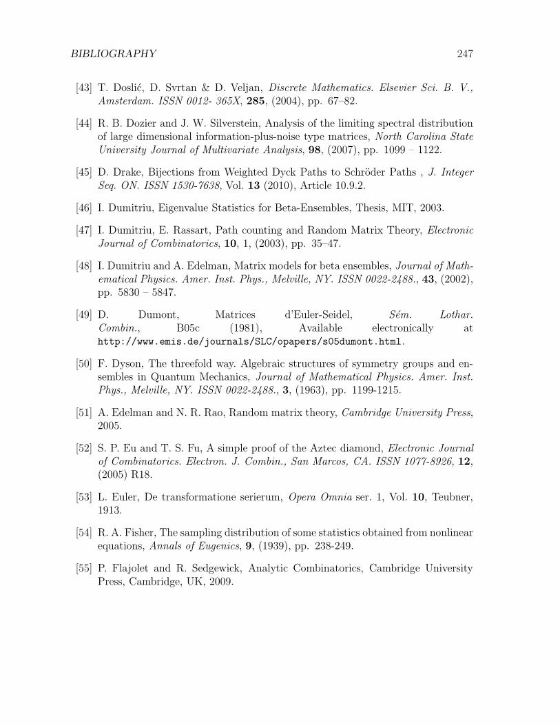
BIBLIOGRAPHY 247
[43] T. Doslic, D. Svrtan & D. Veljan, Discrete Mathematics. Elsevier Sci. B. V.,Amsterdam. ISSN 0012- 365X, 285, (2004), pp. 67–82.
[44] R. B. Dozier and J. W. Silverstein, Analysis of the limiting spectral distributionof large dimensional information-plus-noise type matrices, North Carolina StateUniversity Journal of Multivariate Analysis, 98, (2007), pp. 1099 – 1122.
[45] D. Drake, Bijections from Weighted Dyck Paths to Schroder Paths , J. IntegerSeq. ON. ISSN 1530-7638, Vol. 13 (2010), Article 10.9.2.
[46] I. Dumitriu, Eigenvalue Statistics for Beta-Ensembles, Thesis, MIT, 2003.
[47] I. Dumitriu, E. Rassart, Path counting and Random Matrix Theory, ElectronicJournal of Combinatorics, 10, 1, (2003), pp. 35–47.
[48] I. Dumitriu and A. Edelman, Matrix models for beta ensembles, Journal of Math-ematical Physics. Amer. Inst. Phys., Melville, NY. ISSN 0022-2488., 43, (2002),pp. 5830 – 5847.
[49] D. Dumont, Matrices d’Euler-Seidel, Sem. Lothar.Combin., B05c (1981), Available electronically athttp://www.emis.de/journals/SLC/opapers/s05dumont.html.
[50] F. Dyson, The threefold way. Algebraic structures of symmetry groups and en-sembles in Quantum Mechanics, Journal of Mathematical Physics. Amer. Inst.Phys., Melville, NY. ISSN 0022-2488., 3, (1963), pp. 1199-1215.
[51] A. Edelman and N. R. Rao, Random matrix theory, Cambridge University Press,2005.
[52] S. P. Eu and T. S. Fu, A simple proof of the Aztec diamond, Electronic Journalof Combinatorics. Electron. J. Combin., San Marcos, CA. ISSN 1077-8926, 12,(2005) R18.
[53] L. Euler, De transformatione serierum, Opera Omnia ser. 1, Vol. 10, Teubner,1913.
[54] R. A. Fisher, The sampling distribution of some statistics obtained from nonlinearequations, Annals of Eugenics, 9, (1939), pp. 238-249.
[55] P. Flajolet and R. Sedgewick, Analytic Combinatorics, Cambridge UniversityPress, Cambridge, UK, 2009.

BIBLIOGRAPHY 248
[56] P. Flajolet, Combinatorial aspects of continued fractions, Discrete Mathematics.Elsevier Sci. B. V., Amsterdam. ISSN 0012- 365X , Vol. 32, (1980), pp. 125–161.
[57] S. Fomin, N. Reading, Root Systems and Generalized Associahedra, publishedelectronically at http://arxiv.org/abs/math/0505518, 2005.
[58] G. J. Foschini, Layered Space-Time Architecture for Wireless Communication ina Fading Environment When Using Multi-Element Antennas, Bell LaboratoriesTechnical Journal, (1996), pp. 41-59.
[59] G. J. Foschini and M. J. Gans, On limits of wireless communications in a fadingenvironment when using multiple antennas, Wireless Personal Communications,Vol. 6, No. 3, (1998): pp. 311–335.
[60] G. J. Foschini, G. D. Golden, R. A. Valenzuela and P. W. Wolniansky, Simpli-fied Processing for High Spectral Efficiency Wireless Communication EmployingMulti-Element Arrays, IEEE Journal on Selected Areas in Communications, Vol.17, No. 11, (1999), pp. 1841–1852.
[61] P. di Francesco, Matrix model combinatorics: Applications to colouring andfolding, in Random matrix models and their applications, Cambridge Univer-sity Press (2001), pp. 111–170.
[62] W. Gautshi, Orthogonal polynomials applications and computation, Acta Nu-merica 1996, Cambridge University Press, (1996), pp. 45–119. MR 99i:65019.
[63] W. Gautschi, Orthogonal Polynomials: Computation and Approximation, Claren-don Press, Oxford, 2003.
[64] S. Getu, L.W. Shapiro and W.J. Woan, The Riordan group, Discrete Mathemat-ics. Elsevier Sci. B. V., Amsterdam. ISSN 0012- 365X , 34, (1991), pp. 229–239.
[65] I. Groh, S. Plass & S. Stand, Capacity approximation for uncorrelated MIMOchannels using random matrix methods In Proc. 2006 Second International Sym-posium on Communications, Control and Signal Processing, Marrakech, Morocco,(2006), pp. 13–16.
[66] A Guionnet, Large Random Matrices: Lectures on Macroscopic Asymptotics,cole d’t de Probabilits de Saint-Flour XXXVI, 2006.
[67] M. C. Harding, Explaining the Single Factor Bias of Arbitrage Pricing, Ecco-nomics letters, 2007.

BIBLIOGRAPHY 249
[68] M. C. Harding, Structural Estimation of High-Dimensional Factor Models un-covering the Effect of Global Factors on the US Economy, Job Market Paper,2007.
[69] G. Heinig , Chebyshev-Hankel matrices and the splitting approach for centrosym-metric Toeplitz-plus-Hankel matrices, Linear Algebra and its Applications. ISSN0024-3795., Vol. 327, Issues (1-3), (2001), pp. 181–196.
[70] S. Heubach & T. Mansour, Staircase tilings and lattice paths, Congr. Numer.182 (2006), pp. 97–109.
[71] B. Holter, J.E. Hakegard & T.A. Myrvoll, On the use of MIMO in aeronauticalcommunications, ENRI Int. Workshop on ATM, 2010.
[72] P. L. Hsu, On the distribution of roots of certain determinantal equations, Annalsof Eugenics, Vol. 9 (1939), pp. 250–258.
[73] K. Johansson, Non-intersecting paths, random tilings and random matrices, Prob-ability Theory Related Fields, Vol. 123, (2002), pp. 225–280.
[74] O. Khorunzhiy, Rooted trees and moments of large sparse random matrices,Discrete Mathematics and Theoretical Computer Science, Vol. AC, (2003), pp.145–154.
[75] V. P. Kostov, A. Martınez-Finkelshtein & B. Z. Shapiro, Narayana numbers andSchur-Szego composition, Journal of Approximation Theory, Vol. 161, Issue 2,(2008), pp. 464–476.
[76] C. Krattenthaler, Advanced Determinant Calculus, Seminaire Lotharingien Com-bin. (B42q), 42, 1999.
[77] L. Laloux, P. Cizeau and M. Potters and J.P. Bouchaud, Random matrix the-ory and financial correlations, International Journal of Theoretical and AppliedFinance, Vol. 3 No. 3, (2000), pp. 391–397.
[78] J. W. Layman, The Hankel Transform and Some of its properties, J. Integer Seq.,Waterloo, ON. ISSN 1530-7638, 4, (2001), Article 01.1.5.
[79] F. Lehner, Culmulants, Lattice paths and orthogonal polynomials,Discrete Math-ematics. Elsevier Sci. B. V., Amsterdam. ISSN 0012- 365X, Vol. 270, (2003),pp. 177–191.

BIBLIOGRAPHY 250
[80] F. Lehner, Free cumulants and enumeration of connected partitions, Europ. J.Combin. 22, Vol. 270,(2002), pp. 1025–1031.
[81] N. A. Loehr, Bijective Combinatorics, CRC Press, Boca Raton, 2011.
[82] B. Mckay, The expected eigenvalue distribution of a large regular graph, LinearAlgebra and its Applications. ISSN 0024-3795, 40, (1981), pp. 203 – 216.
[83] V. A. Marcenko and L.A. Pastur, Distribution of eigenvalues for some sets ofrandom matrices, Math. USSR, Sb., Vol. 1, No. 4, (1967), pp. 457–483.
[84] M. L. Mehta, Random Matrices, Academic Press, Boston, third edition, 1991.
[85] D. Merlini and M.Verri, Generating trees and proper Riordan arrays, DiscreteMathematics. Elsevier Sci. B. V., Amsterdam. ISSN 0012-365X , 218, (2000),pp. 167–183.
[86] D. Merlini , The tennis ball problem, Journal of Combinatorial Theory. SeriesA. Elsevier, Inc., Amsterdam. ISSN 0097-3165., Series A, Vol. 99, (2002), pp.307–344.
[87] D. Merlini and R.Sprugnoli, A Riordan array proof of a curious identity, J. IntegerSeq., Waterloo, ON. ISSN 1530-7638, 2 A8, 2002.
[88] D. Merlini, R. Sprugnoli and M. Verri, Combinatorial sums and implicit Riordanarrays, Discrete Mathematics. Elsevier Sci. B. V., Amsterdam. ISSN 0012-365X.,Vol. 309, Issue 2, (2009), pp. 475–486.
[89] D. Merlini, R. Sprugnoli and M. C. Verri, Lagrange Inversion: When and How,Acta Applicandae Mathematicae, 94, (2006), pp. 233–249.
[90] D. Merlini, R. Sprugnoli and M. C. Verri, The Method of Coefficients, Amer.Math. Monthly, 114, (2007), pp. 40–57.
[91] I. Mezo and A. Dil, Euler-Seidel method for certain combinatorial numbers and anew characterization of Fibonacci sequence, Central European Journal of Math-ematics. Versita, Warsaw. ISSN 1895-107, Vol. 7, No. 2, (2009), pp. 310–321.
[92] S. J. Miller, Notes on Random matrix theory, 2004.
[93] S. J. Miller and R. Takloo - Bighash, Introduction to Random matrix theory inInvitation to Modern number theory, Princeton University Press, 2007.

BIBLIOGRAPHY 251
[94] R. Muller, A Random Matrix Model of Communications via Antenna Arrays,IEEE Transactions on Information Theory, Vol. 48, No. 9, (2002) , pp. 2495–2506.
[95] R. Muller, D. Guo & A. Moustakas, Vector precoding for wireless MIMO systemsand its replica analysis, IEEE Journal on Selected Areas in Communications, Vol.26, No. 3, (2008), pp. 530–540.
[96] B.M. Zaidel, R. Muller, A.L. Moustakas, R. de Miguel, Vector Precoding forGaussian MIMO Broadcast Channels: Impact of Replica Symmetry Breaking,published electronically at http://arxiv.org/abs/1001.3790, 2011.
[97] R. J. Muirhead, Aspects of Multivariate Statistical Theory, John Wiley and Sons,New York, 1982.
[98] J. A. Nossek, M. Joham, and W. Utschick Transmit Processing in MIMO WirelessSystems, IEEE 6th CAS Symp. on Emerging Technologies: Mobile and WirelessCommunication, 2005.
[99] A. Okounkov, Random matrices and random permutations, International Math-ematical Res. Notices, No. 20, (2000), pp. 1043–1095.
[100] A. M. Odlyzko, On the distribution of spacings between zeros of the zeta function.Dynamical, Spectral and Arithmetic Zeta-Functions, Contemporary MathematicsSeries, Vol. 290, (2001),pp. 139–144.
[101] L. Pastur and V. Vasilchuk, On the Law of Addition of Random Matrices,Centrede Physique Theorique de CNRS, 2000.
[102] D. Paul and J. W. Silverstein No eigenvalues outside the support ofthe limiting empirical spectral distribution of a separable covariance ma-trix. Journal of Multivariate Analysis 100, available electronically athttp://www4.ncsu.edu/ jack/pub.html, (2009), pp. 37-57.
[103] P. Peart, W-J. Woan, Generating Functions via Hankel and Stieltjes Matrices,J. Integer Seq., Waterloo, ON. ISSN 1530-7638, Vol. 3, (2000), Article 00.2.1.
[104] P. C. Phillips Proffessor T. W. Anderson interview, Ec-conometric theory, 2, 249-288, available electronically athttp://korora.econ.yale.edu/phillips/pubs/art/i002.pdf, 1986.
[105] A. Postnikov, V. Reiner & L. Williams, Faces of Generalized Permutohedra,Documenta Math., 13, (2008) pp. 207–273.

BIBLIOGRAPHY 252
[106] W. H. Press, S. A. Teukolsky, W. T. Vetterling, B. P. Flannery, Numerical recipesin C. The art of scientific computing, University press, Cambridge, 2nd Ed., 1992.
[107] A. Owczarek, T. Prellberg, Enumeration of area-weighed Dyck paths with re-stricted height, published electronically at http://arxiv.org/abs/1004.1699,2010.
[108] R. Brak, G.K Iliev, T. Prellberg, An infinite family of adsorptionmodels and restricted Lukas iewicz paths, published electronically athttp://arxiv.org/abs/1105.0306, 2010.
[109] C. Radoux, Calcul effectif de certains determinants de Hankel, Bulletin de laSociete Mathematique de Belgique, 1979.
[110] R. Rao, The Mathematics of Infinite Random Matrices the Stieltjes transformbased approach, Lectures from MIT, 2004.
[111] B. Riemann, Uber die Anzahl der Primzahlen unter einer gegebenen Grosse,Monatsberichte der Berliner Akademie, 1859.
[112] T. Rivlin, Chebyshev polynomials: from approximation theory to algebra andnumber theory, 2. ed., Wiley, New York, 1990.
[113] B. Rosenow, V. Plerou, P. Gopikrishnan, Amaral and H. Eugene Stanley, ap-plication of random matrix theory to study cross - correlations of stock prices,International Journal of Theoretical and Applied Finance, Vol. 3, No. 3, (2000),pp. 399–403.
[114] C. Shannon A Mathematical Theory of Communication, Bell System TechnicalJournal, 1948.
[115] L. W. Shapiro, Bijections and the Riordan group, Theoretical Computer Science.Elsevier B. V., Amsterdam. ISSN 0304-3975, Vol. 307, (2003), pp. 403–413.
[116] R. Sprugnoli, Riordan Array Proofs of Identities in Gould’s Book,http://www.dsi.unifi.it/resp/GouldBK.pdf, 2006.
[117] R. Sprugnoli, A bibliography of Riordan arrays,http://www.dsi.unifi.it/ resp/BibRioMio.pdf, 2011.
[118] L. W. Shapiro, S. Getu, W-J. Woan and L.C. Woodson, The Riordan Group,Discrete Applied Mathematics. The Journal of Combinatorial Algorithms, In-formatics and Computational Sciences. Elsevier Sci. B. V., Amsterdam. ISSN0166-218X, Vol. 34, (1991), pp. 229–239.

BIBLIOGRAPHY 253
[119] L. W. Shapiro, S. Getu, W.-J. Woan and L. Woodson, The Riordan Group,Discrete Applied Mathematics. The Journal of Combinatorial Algorithms, In-formatics and Computational Sciences. Elsevier Sci. B. V., Amsterdam. ISSN0166-218X, Vol. 34, (1991), pp. 229–239.
[120] L. Shapiro, Bijections and the Riordan group, Theoretical computer science, Vol.307, (2003), pp. 403 – 413
[121] L. Shapiro, A survey of the Riordan Group, Talk at a meeting of the AmericanMathematical Society, 1994.
[122] L. Shapiro, The uplift principle and the Riordan group, Talk at the KAISTDiscete maths seminar, 2011.
[123] J. W. Silverstein, Z. D. Bai, On the Empirical Distribution of Eigenvalues of aClass of Large Dimensional Random Matrices, J. of Multivariate Analysis, Vol.54, (1995), pp. 175–192.
[124] N. J. A. Sloane, The On-Line Encyclopedia of Integer Sequences. Published elec-tronically at http://www.oeis.org, 2011.
[125] N. J. A. Sloane, The On-Line Encyclopedia of Integer Sequences, Notices of theAMS, 50, (2003), pp. 912–915.
[126] P. Sniady, Permutations without long decreasing subsequences and random ma-trices, University of Wroclaw, 2007.
[127] R. Speicher, Free convolution and the random sum of matrices, Research Institutefor Mathematical Sciences, Vol. 29, (1993), pp. 731–744.
[128] R. Speicher, Multiplicative functions on the lattice of non-crossing partitions andfree convolution, Annals of Mathematics, Vol. 298, (1994), pp. 611–620.
[129] R. Speicher, Combinatorial theory of the free product with amalgamation andoperator-valued free probability theory,Memoirs of the American Mathematicalsociety, 627, 1998.
[130] N. J. A. Sloane, My favorite integer sequences, a paper for the SETA’98 confer-ence on sequences, 1998.
[131] R. Sprugnoli, Riordan arrays and combinatorial sums, Discrete Mathematics.Elsevier Sci. B. V., Amsterdam. ISSN 0012-365X, Vol. 132, (1994), pp. 267–290.

BIBLIOGRAPHY 254
[132] R. Sprugnoli , R. Sprugnoli, Riordan arrays and combinatorial sums, DiscreteMathematics. Elsevier Sci. B. V., Amsterdam. ISSN 0012- 365X, Vol. 132(1994),pp. 267–290.
[133] R. Sprugnoli, A unified approach to combinatorial sum inversion, Technical Re-port RT 14/94, Dipartimento Sistemi e Informatica, 1994.
[134] R. Sprugnoli, An Introduction to Mathematical Methods in Combinatorics,http://www.dsi.unifi.it/7Eresp/Handbook.pdf, 2006.
[135] R. Sprugnoli, Riordan Array Proofs of Identities in Gould’s Book. Available elec-tronically at http://www.dsi.unifi.it/resp/GouldBK.pdf, 2007.
[136] R. Stanley, Catalan Addendum, available electronically athttp://www-math.mit.edu/ rstan/ec/catadd.pdf, 2011.
[137] R. A. Sulanke, Counting lattice paths by Narayana polynomials, Electronic J.Combin. 7, 2000.
[138] R. A. Sulanke, The Narayana distribution, J. Statist. Plann. and Infer. 101(2002) pp. 311–346.
[139] R. A. Sulanke, Generalizing Narayana and Schroder numbers to higher dimensions,Electron. J. Combin. 11 (1) (2004), #R54.
[140] B. Sutton, The Mathematics of Infinite Random Matrices Tridiagonal Matrices,Orthogonal Polynomials and the Classical Random Matrix Ensembles, Handout,MIT lectures, 2004.
[141] Y. Sun, The Star of David rule, published electronically athttp://arxiv.org/abs/0805.1277, 2008.
[142] G. Szego, Orthogonal Polynomials, 4th ed. Providence, RI, Amer. Math. Soc.,(1975).
[143] E. Teletar, The capacity of Gaussian Mult-antenna channels, European Transac-tions on Telecommunications, 10(6), 1999, pp. 585–596.
[144] V. Totik, Orthogonal polynomials, published electronically athttp://arxiv.org/abs/math/0512424v1, 2005.
[145] D. Tse and P. Viswanath, Fundamentals of wireless communications, Cambridgeuniversity press, 2005.

BIBLIOGRAPHY 255
[146] A. Tulino, S. Verdu, Random Matrix Theory and Wireless Communications, nowPublishers Inc., Hanover, MA., 2004
[147] S. Verdu and S. Shamai, Spectral Efficiency of CDMA with Random Spreading,IEEE Trans. Information Theory, Vol. 45,, No. 2, (1999), pp. 622–640.
[148] S. Verdu and Tulino, Random Matrix theory and wireless communications, NowPublisher Inc,ISSN:1567-2190, 2004.
[149] S. Verdu, Random Matrix Theory and its applications to Statistics and Wire-less Communications Eigenvalues and Singular Values of Random Matrices: ATutorial Introduction, Princeton University, National University of Singapore,Institute for Mathematical Sciences, 2006.
[150] S. Verdu, Workshop on Random Matrix Theory and Wireless Communications,The Interplay between Random Matrices and Information Theory ChautauquaPark, Boulder, Colorado, Princeton University, 2008.
[151] X. Viennot, Une theorie combinatoire des polynomes orthogonaux generaux, Lec-ture notes, UQAM, Montreal, Quebec, 1983.
[152] D. Voiculescu, Addition of certain non-commuting random variables, Journal ofFunctional Analysis, 66, pp. 323–346, 1986.
[153] D. Voiculescu, Limit laws for random matrices and free products, In-vent.math.,104, (1991), pp. 201–220.
[154] D. Voiculescu, Free probability theory: random matrices and von Neumannalge-bras, Proceedings of the ICM 1994, Birkhauser, (1995), pp. 227–241.
[155] D. Voiculescu, Free Probability Theory, Fields Institute Communications, Vol.12, 1997.
[156] H. S. Wall, Analytic Theory of Continued Fractions, Chelsea publishing company,1948.
[157] E. Weisstein, Morgan-Voyce Polynomials, MathWorld, available electronically athttp://mathworld.wolfram.com/Morgan-VoycePolynomials.html, 2009.
[158] H. Widom, On the Limiting Distribution for the Longest Alternating Sequencein a Random Permutation, Department of Mathematics University of California,2005.

BIBLIOGRAPHY 256
[159] E. Wigner, Characteristic vectors of bordered matrices with infinite dimensions,Annals of Mathematics, Vol. 62, (1952), pp. 546 –564.
[160] A. S. Wightman, Eugene Paul Wigner 1902-1995, Notices of the American Math-ematical Society, 1995.
[161] H. S. Wilf, Generatingfunctionology, department of Mathematics, University ofPennsylvania, Pennsylvania,1990.
[162] H. S. Wilf, The Longest increasing sub-sequences in pattern-restricted permuta-tions, Electronic Journal of Combinatorics. Electron. J. Combin., San Marcos,CA. ISSN 1077-8926 v9 i2. R12, 2003.
[163] J. Wishart, On the multivariate distribution in samples from a multivariate pop-ulation, Vol. 62, (1952), pp. 546 – 564.
[164] W.-J. Woan, Hankel matrices and lattice paths, J. Integer Seq., Waterloo, ON.ISSN 1530-7638, Vol. 4 (2001), Article 01.1.2.
[165] H. Widom, Homepage of Harold Widom available electronically athttp://math.ucsc.edu/ widom/widom.html,2011.
[166] D. Zeilberger, Six etudes in generating functions, International Journal of Com-puter Mathematics, 29, (2-4) (1989), pp. 201–215.
[167] American Statistical society website available electronically athttp://www.ams.org/, 2011.
[168] Biography on the Institut de Physique Theorique website, available electronicallyat available electronically at http://ipht.cea.fr/en/Phocea-SPhT/, 2011.
[169] School of Mathematics and Statistics, University of St. An-drews, Scotland, Biographies, available electronically athttp://www-history.mcs.st-andrews.ac.uk.,2011


![Riordan Arrays, Orthogonal Polynomials as Moments, and ......sequences, generating functions, orthogonal polynomials [5, 12, 30], Riordan arrays [25, 29], production matrices [10,](https://static.fdocuments.us/doc/165x107/60f808d5fc519a150d61ac4d/riordan-arrays-orthogonal-polynomials-as-moments-and-sequences-generating.jpg)


