A stress-based approach

to the solution of

Saint Venant problem

Ph.D. Dissertation

Sergio Guarino

Corso di Dottorato di Ricerca in Ingegneria delle Costruzioni, XXIV ciclo

Dipartimento di Ingegneria Strutturale

Universita di Napoli Federico II

Via Claudio, 21 - 80125 Napoli

e-mail: sergio.guarino@unina.it

November, 2011

Tutor: Coordinatore del corso:

Prof. L. Rosati Prof. F. Mazzolani

1

Acknowledgements

The present research work has been carried out at the Department of Struc-

tural Engineering (DIST) of the University of Naples Federico II.

I am indebted to many people for their support and encouragement while

preparing this dissertation and I would like to record my acknowledgements to

the following: to prof. Luciano Rosati, supervisor of the present work, for his

interest and care; to all of my colleagues for their suggestions and interesting

discussions; and finally, to my friends and my family, without whose love and

support this work could not have been done.

Naples, November 2011

SERGIO GUARINO

2

Contents

1 Introduction 7

2 Beltrami-Michell equation 13

2.1 Background . . . . . . . . . . . . . . . . . . . . . . . . . . . . . 13

2.1.1 Vector product of vectors and tensors . . . . . . . . . . 14

2.1.2 Tensor product of second-order tensors . . . . . . . . . . 17

2.1.3 Derivatives . . . . . . . . . . . . . . . . . . . . . . . . . 17

2.2 The pseudo-vectorial operator ∇ and symbolic differential cal-

culus . . . . . . . . . . . . . . . . . . . . . . . . . . . . . . . . . 18

2.3 Compatibility . . . . . . . . . . . . . . . . . . . . . . . . . . . . 23

2.4 Bianchi identities . . . . . . . . . . . . . . . . . . . . . . . . . . 28

2.5 Rivlin identities . . . . . . . . . . . . . . . . . . . . . . . . . . . 29

2.5.1 First Rivlin Identity . . . . . . . . . . . . . . . . . . . . 30

2.5.2 Second Rivlin Identity . . . . . . . . . . . . . . . . . . . 31

2.5.3 Third Rivlin identity . . . . . . . . . . . . . . . . . . . . 31

2.6 Specialization of Rivlin identities to the case of skew-symmetric

tensors . . . . . . . . . . . . . . . . . . . . . . . . . . . . . . . . 32

2.7 Field equations of linear isotropic elasticity . . . . . . . . . . . 33

2.8 Beltrami-Michell equation . . . . . . . . . . . . . . . . . . . . . 35

3 Saint Venant problem 39

3

3.1 Saint Venant hypothesis . . . . . . . . . . . . . . . . . . . . . . 40

3.2 Stress field in the Saint-Venant theory . . . . . . . . . . . . . . 42

3.3 Stress field associated with torsion . . . . . . . . . . . . . . . . 46

3.4 Frame-independent representation of the stress field associated

with pure shear . . . . . . . . . . . . . . . . . . . . . . . . . . . 47

3.5 Tangential stress field . . . . . . . . . . . . . . . . . . . . . . . 51

3.6 De Saint Venant stress field expressed in terms of internal forces 51

3.6.1 The torsional stiffness factor . . . . . . . . . . . . . . . 53

3.7 Closed-form analytical solutions . . . . . . . . . . . . . . . . . . 54

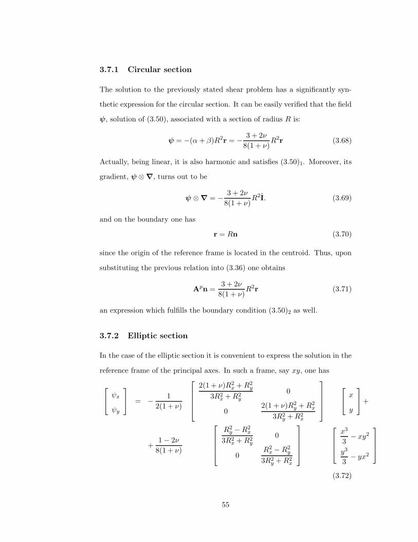
3.7.1 Circular section . . . . . . . . . . . . . . . . . . . . . . . 55

3.7.2 Elliptic section . . . . . . . . . . . . . . . . . . . . . . . 55

3.7.3 Rectangular section (ν = 0) . . . . . . . . . . . . . . . . 56

4 Displacement field, shear center and deformability tensor 57

4.1 Derivation of the displacement field . . . . . . . . . . . . . . . . 57

4.1.1 Displacement field associated with axial force . . . . . . 58

4.1.2 Displacement field associated with biaxial bending . . . 59

4.1.3 Displacement field associated with torsion . . . . . . . . 61

4.1.4 Displacement field associated with biaxial shear . . . . . 64

4.2 Shear center . . . . . . . . . . . . . . . . . . . . . . . . . . . . . 69

4.2.1 Boundary integral tensor expression of the shear center 71

4.2.2 Further developments for polygonal sections . . . . . . . 72

4.3 Frame-independent form of the shear flexibility tensor . . . . . 73

4.3.1 Expression of the shear flexibility tensor by means of

boundary integrals . . . . . . . . . . . . . . . . . . . . . 74

4.3.2 Shear flexibility tensor for the circular section . . . . . . 79

4.4 Stiffness tensor of a beam element . . . . . . . . . . . . . . . . 80

4

5 A BEM approach to the solution of the torsion and shear

problems 83

5.1 Weak formulation . . . . . . . . . . . . . . . . . . . . . . . . . . 84

5.2 Interpolation . . . . . . . . . . . . . . . . . . . . . . . . . . . . 85

5.3 Algebraic solution system . . . . . . . . . . . . . . . . . . . . . 86

5.4 Entries of the solution system matrix . . . . . . . . . . . . . . . 88

5.5 Calculus of ψ for points located at the interior of the domain . 94

5.6 Calculus of derivatives of ψ for points located at the interior of

the domain . . . . . . . . . . . . . . . . . . . . . . . . . . . . . 97

6 Numerical results 99

6.1 Rectangular cross section . . . . . . . . . . . . . . . . . . . . . 100

6.2 Circular cross section . . . . . . . . . . . . . . . . . . . . . . . . 103

6.3 L-Shaped cross section . . . . . . . . . . . . . . . . . . . . . . . 105

6.4 Trapezoidal cross section . . . . . . . . . . . . . . . . . . . . . . 107

6.5 C-Shaped cross section . . . . . . . . . . . . . . . . . . . . . . . 110

6.6 A section of arbitrary polygonal shape . . . . . . . . . . . . . . 113

7 Appendix 115

7.1 Examples of application of the Gibbs rule . . . . . . . . . . . . 115

7.2 Matrix representation of the fourth-order tensor Wa Wa . . 121

7.3 Baldacci’s frame-dependent representation of the shear stress

field . . . . . . . . . . . . . . . . . . . . . . . . . . . . . . . . . 123

7.4 Further identities . . . . . . . . . . . . . . . . . . . . . . . . . . 126

7.4.1 Proof of identity (7.16) . . . . . . . . . . . . . . . . . . 126

7.4.2 Proof of identity (4.92) and (4.92) . . . . . . . . . . . . 127

7.4.3 Proof of identity (4.96) . . . . . . . . . . . . . . . . . . 127

7.4.4 Proof of identity (4.97) . . . . . . . . . . . . . . . . . . 128

7.5 Nomenclature . . . . . . . . . . . . . . . . . . . . . . . . . . . . 129

5

6

Chapter 1

Introduction

The solution to Saint-Venant problem, concerning the elastic equilibrium prob-

lem of beams, is classically addressed by the displacement approach. Still to

date, more than one hundred and fifty years since the publication of the two

fundamental papers by A.J.C. Barre de Saint Venant [4, 5], the solution of this

classical problem is derived by adopting the celebrated semi-inverse approach

pioneered by the french mathematician, and is classically taught in the form

contributed by Clebsch [17].

At a first sight the displacement approach appears to be straightforward

and effective, basically for two reasons: the Cauchy-Navier equations, govern-

ing the elastic equilibrium problem of solids in which the displacement field is

the primary unknown, are easier to derive and by far simpler with respect to

the corresponding ones, due to Beltrami and Michell [9, 40], which formulate

the elastic equilibrium problem in terms of the stress field.

Moreover, a solution expressed in terms of stresses would require an inte-

gration procedure to derive the corresponding displacement field, as opposite

to the straightforward differentiation procedure which allows one to derive the

stress field once the displacement field has been assigned.

Only one hundred years after Saint-Venant papers Riccardo Baldacci [6],

7

professor of Scienza delle Costruzioni (the italian acronym for Structural and

Solid Mechanics) at the University of Genova, presented a stress-based for-

mulation of the elastic equilibrium problem of beams which turn out to be

particularly compact and elegant.

In the author’s opinion the main reason which makes Baldacci treatment

preferable to the classical one is that there is no need to figure out the displace-

ment field and to check a posteriori its correctness according to Saint-Venant

semi-inverse method.

Conversely, the stress field solution of de Saint-Venant problem is directly

and consistently derived from Beltrami-Michell equation without invoking any

a-priori assumption apart from the classical hypotheses which characterize

Saint-Venant model of beams.

The price to pay for using the approach pioneered by Baldacci is that the

displacement field solution of Saint-Venant problem is not easy to derive since

it requires to integrate the strain field associated with stress field via the linear

isotropic elastic law.

However, it is shown in the dissertation that this issue, not addressed by

Baldacci, can be solved elegantly and in full generality by an integration pro-

cedure, basically equivalent to Cesaro’s formula, which can be applied indif-

ferently, though with a different degree of complexity, to any kind of internal

force, that is axial force, torsion, biaxial bending and biaxial shear.

In order to achieve this result the original treatment of Saint-Venant prob-

lem due to Baldacci is reformulated more synthetically by an extensive use of

tensor calculus.

In this respect use is made of an original derivation of Beltrami-Michell

equation which can be defined of algebraic nature in the sense that the fi-

nal result is obtained by means of basic operations of tensor calculus which

formally replace the differential manipulations usually exploited in classical

8

textbooks of continuum mechanics.

Basically these manipulations are of two kinds: the first one, mainly co-

incident with that initially formulated by Beltrami [9] and later generalized

by Michell [40], hinges on the systematic use of the indicial notation and, in

particular, of the ε − δ identities connecting Ricci tensor to the identity one.

The second approach [29] to the derivation of Beltrami-Michell equations ba-

sically reformulates the above-mentioned identities in intrinsic form by means

of tensor identities which are very elegant but completely hinder the meaning

and the consequentiality of the several not-trivial steps required to achieve the

final result.

It is shown, on the contrary, that the approach illustrated in this disserta-

tion makes the whole procedure transparent though formally involved.

Basically, it is based on the extensive use of Gibbs calculus to formally

address gradient, divergence, curl and Laplace operator of vector or tensor

fields by applying the rules of tensor calculus to the field and to a fictitious

vector known as the ∇ (nabla) operator by Hamilton.

A suitable extension of classical Gibbs calculus is presented in the disser-

tation by introducing an original definition of vector product between vectors

and tensors which is required to derive more elaborate results.

Following this approach the compatibility conditions for the infinitesimal

strain field as well as Bianchi identities can be derived elegantly and in a

straightforward manner. Moreover, invoking Rivlin identities [46], Beltrami-

Michell equations are obtained by a constructive approach in which any step

of the procedure follows naturally and consequentially from the previous one.

Accordingly, the dissertation is basically divided in two main parts. The

first one includes the above mentioned issues on differential calculus while

the second one is completely devoted to the tensor reformulation of Baldacci

approach to Saint-Venant problem and to the presentation of some original

9

results. The first one, as previously specified, is concerned with the explicit

derivation, in tensor form, of the displacement field, separately for axial force,

torsion, biaxial bending and biaxial shear. Since the reference frame is com-

pletely arbitrary no a priori use of the inertia principal directions is required

for addressing bending and shear.

The second original result presented in the dissertation is represented by

a frame-independent solution of the shear problem which, to the best of the

author’s knowledge, has not yet been proposed. For instance, the matrix

field used by Baldacci to implicitly define the shear stress solution does not

constitute the matrix representation of a tensor field. The same drawback

holds as well for the shear center in the sense that, differently from the centroid,

it is not yet available a frame-independent expression of the shear center; the

same comment applies also to the shear flexibility tensor and to the shear

factor tensor.

In the light of the considerations pointed out above, a solution method for

the determination of the shear stress field, alternative to the treatment by

Baldacci [6], is illustrated in the dissertation thus allowing to represent the

stress field, as well as the displacement one, in a completely intrinsic form.

The proposed formulation of the shear problem is based on the solution

of the Neumann problem associated with the shear stress field which is ob-

tained by exploiting an intrinsic particular integral of the differential problem

emerging from Baldacci’s approach to Saint-Venant problem. In this way the

representation obtained for the shear stress field, for the shear center and for

the shear flexibility tensor presents the advantage of being independent from

the particular reference frame and of being written in intrinsic, and hence

more synthetic, form.

As a final contribution the numerical solution of shear and torsion problem

is carried out by a novel BEM approach in which only the vertices of the cross

10

section, assumed to be polygonal, need to be assigned. In this way the input

data required for analyzing the cross section subject to any kind of internal

force are identical to those traditionally employed for axial force and biaxial

bending.

11

12

Chapter 2

Beltrami-Michell equation

In this chapter it will be shown that the basic set of differential relations of the

stress-based formulation of linear isotropic elastostatics can be derived by a

constructive approach based upon an algebraic path of reasoning. The result

will be obtained by extending Gibbs symbolic calculus to tensor fields and in-

troducing an original definition of vector product between vectors and second-

order tensors. In particular, an algebraic reformulation of the compatibility

condition for the linearized strain tensor, made possible by the exploitation of

Rivlin’s identities for tensor polynomials, allow one to derive Beltrami-Michell

equation by a direct approach. The same considerations do apply as well to

the Saint Venant compatibility condition and to Bianchi identity.

2.1 Background

Given a three- or two-dimensional inner product space V over the reals, one

denotes by Lin the space of linear transformation (second-order tensors) on V

, and by Lin the space of all tensors on Lin. Unless differently stated, elements

of V and Lin will be denoted respectively by lowercase, e.g. a, and uppercase,

e.g. A, bold symbols; furthermore fourth-order tensors, which represent the

13

elements of Lin, will be denoted by boldblackboard uppercase symbols, e.g.

A.

Well-known composition rules involving vectors and tensors are:

Ab · c = b ·Atc = A · (c⊗ b) (2.1)

where (·)t stands for transpose, and:

A(b⊗ c) = Ab⊗ c (b⊗ c)A = b⊗Atc (2.2)

see, e.g., [29].

This chapter introduces in particular the definition of vector product be-

tween vectors and second-order tensors and presents some of its properties; in

addition some properties of tensor products between second-order tensors and

basic results of differential calculus for tensors valued functions of tensors will

be briefly reviewed.

2.1.1 Vector product of vectors and tensors

It is well-known [14] that there exists a one-to-one correspondence between

vectors and skew-simmetric tensors which is expressed by:

a× b = Wab ∀b ∈ V. (2.3)

Assuming that the argument b in the previous relationship represents the

result of a linear transformation T : V→ V one has:

a× (Sc) = Wa(Sc) = (WaT)c ∀ c ∈ V. (2.4)

Since the left-hand side of the previous relation is linear in c, we can define

the vector product between a vector and a tensor as the linear operator a×T

fulfilling the property:

(a×T)c = a×Tc = (WaT)c ∀ c ∈ V. (2.5)

14

and we write:

a×Tdef= WaT (2.6)

It is interesting to notice that the i-th column of the matrix associated with

a×T in a cartesian frame is simply the vector product between a and the i-th

column of the matrix associated with T. Actually, recalling the composition

rule (2.2), one has:

a×T = a×

3∑

i=1

Tei ⊗ ei =

3∑

i=1

(WaTei)⊗ ei =

3∑

i=1

(a×Tei)⊗ ei (2.7)

This is exactly the definition reported, e.g., in [39].

Using the definition (2.6) one obtains an alternative way of expressing the

relation between a skew tensor and the associated axial vector:

Wa = a× I. (2.8)

We shall also denote by axial the linear operator which associates with every

skew tensor Wa the relevant axial vector a, that is:

axialWa = a (2.9)

in particular, it turns out to be:

axialWta = −axialWa (2.10)

Some additional properties stemming from the definition (2.6) are

a× (b⊗ c) = (a× b)⊗ c (2.11)

an identity addresses in [2], and

a× (b×T)c = a× (b×Tc) (2.12)

Furthermore, using the vector identity:

a× (b× c) = (a · c)b − (a · b)c (2.13)

15

one obtains:

a× (b×T) = (b⊗ a)S− (a · b)S (2.14)

and its trivial specializations:

a× (b× I) = WaWb = (b⊗ a)− (a · b)I (2.15)

a× (a× I) = W2a = (a⊗ a)− (a · a)I (2.16)

Exploiting the anticommutativity property of the vector product one gets

from (2.13) the further identity:

(a× b)× I = b⊗ a− a⊗ b (2.17)

according to (2.8) the previous relation states that:

a× b = −axial(a⊗ b− b ⊗ a) (2.18)

Starting from the interpretation of vector product between vectors and

tensors provided in (2.7) a further product can be defined:

T × adef= −a×T (2.19)

this amounts to set:

(S× a)c = Sc × a (2.20)

since:

Tc × a = −a×Tc = −(a×T)c (2.21)

It will be shown in the next sections that the previous formulas, of purely

algebraic nature, are particularly useful to provide a simple derivation of dif-

ferential identities.

16

2.1.2 Tensor product of second-order tensors

Given A,B ∈ Lin the tensor product A⊗B, usually termed dyadic product,

is the element of Lin such that:

(A⊗B)C = (B ·C)A = tr (BtC)A ∀C∈ Lin (2.22)

where the symbol tr(·) denotes the trace operator.

More recently Del Piero [19] has introduced an additional tensor product

A B between second-order tensors defined by:

(A B)C = ACBt ∀C∈ Lin (2.23)

which will be referred to in the sequel as square tensor product. The previous

product allows one to represent the identity tensor I ∈ Lin as:

I = I I (2.24)

where I is the identity tensor in Lin. The following composition rules can be

shown to hold:

(A B)(C D) = (AC) (BD)

(A B)(C⊗D) = (ACBt)⊗D

(A⊗B)(C D) = A⊗ (CtBD)

(2.25)

for every A,B,C,D ∈ Lin

2.1.3 Derivatives

Let G : Lin → Lin be a tensor valued function of tensors. G is said to be

differentiable at A if there exists a linear transformation DAG(A), called the

derivative of G at A, such that:

G(A + B)−G(A) = DAG(A)[B] + o(B) asB→ 0; (2.26)

DAG(A)[B] represents the value of the derivative DAG(A) on the increment

B. If two tensor valued functions G and K are differentiable at A, their

17

product:

P(A) = G(A)K(A) (2.27)

is also differentiable at A and:

DAP(A)[B] = DAG(A)[B]K(A)+ G(A)DAK(A)[B] (2.28)

Applying the definition (2.28) it is an easy matter to derive the following

derivatives of the powers of A:

DA(A) = I = I I

DA(A2) = A I + I At

DA(A3) = A2 I + I (A2)t + A At

DA(A4) = A3 I + I (A3)t + A2

At + A (A2)t

(2.29)

which share an amazing symmetry in their expressions and are very easy to

remember. We shall also need the derivatives of the three invariants of a

tensor:

IA = trA IIA =1

2[(trA)2 − (trA2)] IIIA = det A

they are given in turn [59] by:

DA(IA) = I DA(IIA) = IAI−At DA(IIIA) = A∗ (2.30)

where the tensor A∗, which fulfills the properties:

A∗At = AtA∗ = IIIAI, (2.31)

represents the cofactor of A.

2.2 The pseudo-vectorial operator ∇ and symbolic

differential calculus

It is well-known [13, 26, 32, 38] that Gibbs notation [24, 25] allows one to ex-

press the most common differential operators by means of the pseudo-vectorial

18

operator ∇ defined in a Cartesian frame by the expression:

∇ =∂

∂xe1 +

∂

∂ye2 +

∂

∂ze3

where e1, e2, e3 are unit vectors directed along the axes.

Introduced by Hamilton in [30], although with a different symbol, and

usually termed nabla operator, definition and properties of the ∇ operator

have been recently extended to orthogonal curvilinear coordinates in [43].

Mainly after Gibbs [24, 25] it has become a common practice to denote the

gradient, divergence, curl and laplacian respectively by the symbols ∇, ∇·,

∇× and ∇ ·∇.

Although the properties and limitations of ∇ symbolic calculus are well es-

tablished, it will be reported hereafter, mainly for completeness, a comparative

presentation of Gibbs terminology and coordinate-free notation of differential

operators as well as some additional properties of symbolic calculus resulting

from the newly introduced definition of vector product between vectors and

tensors.

Referring to [29, 28, 21] for intrinsic definition of differential operators, the

symbolic counterpart for gradient, divergence and curl of (sufficiently smooth)

scalar, e.g. ϕ, and vector, e.g. a, fields are given by:

ϕ∇def= ∇ϕ

def= gradϕ a⊗∇

def= grada

∇ · adef= a ·∇

def= diva ∇× a

def= curla

(2.32)

see also [3].

The extension of the previous definitions to the case of second-order tensor

fields A can be made on the basis of the intrinsic expressions reported in

[29] and of the definition of vector product between vectors and second-order

tensors:

A∇def= divA ∇×At def

= W∇At def= curlA (2.33)

19

accordingly, we define:

∇× (∇×At)t def= W∇(W∇At)t def

= (W∇ W∇)Adef= curl curlA (2.34)

Finally, the laplacian ∆ of a scalar, vector or tensor field is defined by:

(∇ ·∇)ϕdef= div gradϕ

def= ∆ϕ (∇ ·∇)a

def= div grada

def= ∆a

(∇ ·∇)Adef= div gradA

def= ∆A

(2.35)

It is interesting to notice that (∇·∇)ϕ can be formally obtained by applying

Gibbs definition of divergence to the pseudo-vector ∇ϕ and considering the

scalar product of the two ∇’ s involved in the operation. Analogously, one

gets:

∆a = div grada = (a⊗∇)∇ (2.36)

by invoking the definition of tensor product between vectors [14, 29] on the

basis of (2.32)2 and (2.33)1. A similar path of reasoning can be followed for

∆A by defining:

A⊗∇def= gradA (2.37)

as natural extension of (2.32)2.

Furthermore, by applying basic rules of vector calculus to the symbolic

vector ∇, the following identities can be shown to hold:

a×∇ = −∇× a

∇ · (∇× a) = ∇ · (a×∇) = a · (∇×∇) = 0

∇× (a⊗∇) = (∇× a)⊗∇

∇× (∇⊗ a) = (∇×∇)⊗ a = 0

(2.38)

where a is an arbitrary vector field. Specifically, the first one is the anticom-

mutativity property of the vector product while the second one follows from

a well-known property of the mixed triple product; furthermore, the last two

relationships are based upon (2.11), the second one being zero since the vector

product of two identical vectors vanishes.

20

As a consequence of the previous definitions, all standard vectorial identities

can be expressed symbolically in terms of ∇. However, in order to prove such

identities, special care has to be paid when applying the ∇ operator to the

product of two fields since this definitively amounts to formally applying either

the product or the chain rule of differential calculus.

In this respect we quote the illuminating sentence reported at page 77 of

the second volume collecting the scientific papers by Gibbs [25]:

Gibbs rule - ... The principle in all these cases (i.e. composition of scalar

and vector fields) is that if we have one of the operators ∇, ∇·, ∇× prefixed to

a product of any kind, and we make any transformation of the expression which

would be allowable if the ∇ were a vector (viz. by changes in the order of the

factors, in the signs of multiplication, in the parentheses written or implied,

etc.) by which changes the ∇ is brought into connection with one particular

factor, the expression thus transformed will represent the part of the value of

the original expression which result from the variation of that factor.

In order to extend the previous rule to tensor fields, in which the symbolic

operator ⊗∇ basically comes into play, we postulate the following:

Extended Gibbs rule - The composition of scalar, vector or tensor fields

postfixed by the operator ⊗∇ is carried out by complying with Gibbs rule and

bringing each particular factor into direct connection with ⊗∇ provided that

the resulting expression, representing the part of the original formula which

result from the variation of that factor, makes sense.

A practical application of the previous rules, with special emphasis on the

case of tensor fields, is provided in the Appendix A.

Finally it is reported a reformulation, expressed in terms of Gibbs notation,

of two classical theorems on solenoidal vector fields and irrotational tensor

fields. The reader is referred to [29, 21] for analytical details and the traditional

proof.

21

Theorem on Solenoidal Vector Fields Let a be a class C1 solenoidal

vector field

div a = 0 (2.39)

defined on a domain B having a boundary consisting of a simple closed surface.

Then, there exists a class C1 vector field b on B such that

a = curl b (2.40)

A formal way to express the previous result is to observe that, being:

a = diva = ∇ · a = 0 (2.41)

the vector field a has to be perpendicular to ∇. Thus a has to be of the form:

a = ∇× b = curl b (2.42)

what represents the statement of the theorem.

Theorem on Irrotational Tensor Fields Let B be denote a simply-

connected domain and A a tensor field of class CN (N ≥ 1) on B that satisfies

curl A = 0 (2.43)

Then, there exists a single-valued class CN+1 vector field a on B such that

A = grada = a⊗∇ (2.44)

A formal way to reformulate the theorem is to apply the condition

curl A = 0 (2.45)

to an arbitrary (constant) vector field b. We thus get, by means of (2.33)2

(curlA)b = 0 ⇔ W∇Atb = 0 ⇔ ∇×Atb = 0 (2.46)

The last relation implies that Atb has to be parallel to ∇, i.e.:

Atb = α∇ (2.47)

22

for some α. Being the vector field b arbitrary, it has to be

A = a⊗∇ (2.48)

for some vector field a.

The previous review and the examples reported in the Appendix A illustrate

the basic rules and properties which have to adopted in the application of ∇

symbolic calculus.

Additional results stemming from the definition of vector product between

vectors and rank-two tensors introduced in subsection 2.1 as well as a conve-

nient reformulation of the symbolic operator W∇ W∇ appearing in (2.34)

will be presented in the following sections.

2.3 Compatibility

To show a first application of the results presented in the previous section we

shall prove the well known compatibility theorem ensuring the existence, in a

simply connected body, of a single-valued displacement field u associated with

a given strain field through the strain-displacement relation:

E = sym gradu =1

2

[

gradu + (gradu)t]

=1

2(u⊗∇ + ∇⊗ u) . (2.49)

In particular, we shall provide two separate proofs of the theorem: the first

one is more constructive but unavoidably longer than the second one; in turn

this is particularly compact once the properties of Gibbs symbolic calculus are

properly mastered.

Compatibility Theorem The strain field E associated with a class C3 dis-

placement field satisfies the equation of compatibility:

curl curl E = 0 (2.50)

Conversely, given a class CN (N ≥ 2) symmetric tensor field E on a simply-

connected body B, the fulfillment of (2.50) is sufficient to ensure the existence

23

of a single-valued displacement field u of class CN+1 on B such that E and u

satisfy the strain-displacement relation.

Proof Necessary condition (Long version) We have to prove that a symmetric

tensor field expressed in the form (2.49) fulfills the compatibility condition

(2.50). To this end let us re-write the strain displacement relation in the

equivalent form:

E + W = gradu = u⊗∇ (2.51)

and take the curl of both sides:

curl E + curlW = ∇× (u⊗∇)t (2.52)

According to (2.38)4 the right-hand side of the previous relation vanishes so

that:

curl E = −curl W (2.53)

Thus we are led to evaluate the curl of a swek-symmetric tensor; on account

of (2.33) and (2.15) it is given by:

curlW = −W∇W = (ω ·∇)I− (ω ⊗∇) = (divω)I− gradω (2.54)

where ω is the axial vector associated with W.

Since, by definition:

W =1

2(u⊗∇−∇⊗ u) (2.55)

we get from formula (2.18) and property (2.38)1

ω = axial W = axial

[

1

2(u⊗∇−∇⊗ u)

]

= −1

2u×∇ =

1

2curlu (2.56)

Accordingly:

divω =1

2div (curlu) =

1

2∇ · (∇× u) = 0 (2.57)

on account of (2.38)2 .

24

The previous result, combined with (2.53) and (2.54) yields finally:

curl E = gradω = ω ⊗∇ (2.58)

so that making the curl of the previous result yields finally

curl curl E = curl gradω = ∇× (ω ⊗∇)t = (∇×∇)⊗ ω = 0 (2.59)

where property (2.38)4 has been invoked.

Proof Sufficient condition (Long version) We have to prove that, if a class

CN (N ≥ 2) symmetric tensor field E fulfills the property:

curl curl E = 0 (2.60)

it admits the representation formula (2.49) where u denotes a single-valued

class CN+1 vector field. Setting:

A = curlE (2.61)

the compatibility condition is written equivalently:

curlA = 0 (2.62)

The theorem on irrotational tensor fields, see section 2.2, ensures that, in

a simply-connected domain, it exists a single-valued vector field a ∈ CN such

that:

curl E = A = grad a = a⊗∇ (2.63)

Recalling (2.54) it is natural to consider the curl of the skew tensor Wa asso-

ciated with a:

curlWa = (a ·∇)I− (a⊗∇) = (diva)I− grada (2.64)

so that the sum of (2.63) and (2.64) provides:

curl E + curl Wa = (div a)I (2.65)

25

On the other hand, we get from (2.63),

tr (a⊗∇) = tr (curlE) = tr (W∇Et) = W∇ · E = 0 (2.66)

due to the orthogonality between skew and symmetric tensors. Hence

div a = tr (grada) = tr (a⊗∇) = 0 (2.67)

In conclusion, formula (2.65) supplies

curl (E + Wa) = 0 (2.68)

what ensures, in a simply-connected domain, that

E + Wa = gradu (2.69)

the symmetric part of both sides provides finally the strain-displacement rela-

tion. Finally, the relation between Wa and u can be inferred as in the proof

of the necessity by tracing back formulas from (2.51) to (2.56).

Let us now provide a shorter version of the previous proof.

Alternative proof of the compatibility theorem

Necessary condition (Short version) The necessity of (2.50) follows by con-

sidering the curl of the strain-displacement relation (2.49). Specifically, invok-

ing definition (2.33) one gets:

curlE =1

2curl[(u⊗∇) + (∇⊗ u)] =

=1

2∇× (u⊗∇)t +

1

2∇× (∇⊗ u)t =

=1

2∇× (∇⊗ u) +

1

2∇× (u⊗∇) .

(2.70)

which, on account of (2.38)4 becomes:

curlE =1

2(∇×∇)⊗u+

1

2(∇×u)⊗∇ =

1

2curl (u⊗∇) = ω⊗∇ = gradω.

(2.71)

26

Thus, the curl of the previous relation yields:

curl curlE = curl gradω = ∇× (ω ⊗∇)t =1

2(∇×∇)⊗ω = 0 (2.72)

Sufficient condition (Short version)

The first part of the proof is similar to the one reported in the long version

till formula (2.63). Thus, taking the trace of (2.63) one gets:

div a = a ·∇ = tr (a⊗∇) = tr (curlE) = tr (W∇Et) = W∇ ·E = 0 (2.73)

since E is symmetric and W∇ antysimmetric.

Hence, the theorem on solenoidal tensor fields, see section 2.2, yields:

a = ∇× b (2.74)

which can be substituted in (2.63) to provide:

∇×E = curl E = (∇× b)⊗∇ = ∇× (b⊗∇). (2.75)

on account of property (2.38)3 . Invoking (2.38)4 and being E symmetric one

infers,

E = u⊗∇ + ∇⊗ u (2.76)

where u = b/2

For the purposes of this treatment it is more convenient to reformulate the

equation of compatibility (2.50) by means of the definition (2.34). To further

emphasize the algebraic character of such an expression we report the matrix

representation of the symmetric second-order tensor (curl curlE).

Specifically, invoking formulas (7.10) and (4.45) reported in the appendix

B, we deduce that the six compatibility conditions in a cartesian frame can be

obtained in a straightforward manner by performing a row-by-column product

of the symbolic matrix [W∇ W∇] by the column vector [E] to obtain:

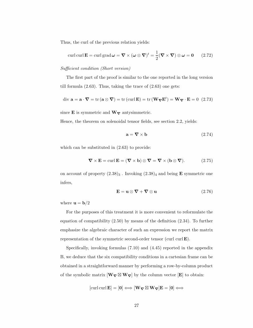
[curl curlE] = [0]⇐⇒ [W∇ W∇]E = [0]⇐⇒

27

0 D33 D22 0 −2D23 0

D33 0 D11 0 0 −2D13

D22 D11 0 −2D12 0 0

0 0 −D12 −D33 D31 D23

−D23 0 0 D13 −D11 D12

0 −D13 0 D23 D12 −D22

E11

E22

E33

E12

E23

E31

= [0] (2.77)

having introducing, for clarity

Dij =∂2

∂xi∂xji, j = 1, 2, 3

Stated equivalently, compatibility equations can be formally obtained by a

trivial matrix multiplication.

2.4 Bianchi identities

To get further evidence of the usefulness of the symbolic calculus presented

in subsection 2.2 it is shown how the so-called Bianchi identities [56] can be

obtained by straightforward manipulations of purely algebraic nature.

The usual way of introducing Bianchi identities in classical textbooks of

continuum mechanics is to observe that the six differential relations embedded

in the compact notation curl curl E = 0 are associated with three displacement

components. This is the hint to realize that the six compatibility conditions

have to be subjected to three independent relations.

Using Gibbs notation Bianchi identities follow immediately:

div( curl curlE) = (W∇EWt∇

)∇ = (W∇

E)(Wt∇

∇) =

= −W∇E(∇×∇) = 0

(2.78)

since the vector product of two ∇’s vanishes as in ordinary vector calculus,

see also (2.38)2 and (2.38)4 .

28

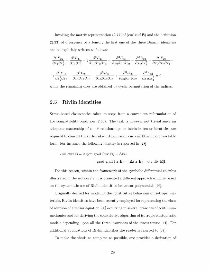
Invoking the matrix representation (2.77) of (curl curl E) and the definition

(2.33) of divergence of a tensor, the first one of the three Bianchi identities

can be explicitly written as follows:

∂3E22

∂x1∂x23

+∂3E33

∂x1∂x22

− 2∂3E23

∂x1∂x2∂x3−

∂3E33

∂x2∂x1∂x2−

∂3E12

∂x2∂x23

−∂3E23

∂x2∂x3∂x1+

+∂3E13

∂x22∂x3

+∂3E22

∂x3∂x1∂x3−

∂3E12

∂x3∂x2∂x3+

∂3E23

∂x3∂x1∂x2−

∂3E13

∂x3∂x22

= 0

while the remaining ones are obtained by cyclic permutation of the indices.

2.5 Rivlin identities

Stress-based elastostatics takes its steps from a convenient reformulation of

the compatibility condition (2.50). The task is however not trivial since an

adequate mastership of ε − δ relationships or intrinsic tensor identities are

required to convert the rather akward expression curl curl E in a more tractable

form. For instance the following identity is reported in [28]

curl curl E = 2 sym grad (div E)−∆E+

−grad grad (tr E) + [∆(tr E)− div div E]I

For this reason, within the framework of the symbolic differential calculus

illustrated in the section 2.2, it is presented a different approach which is based

on the systematic use of Rivlin identities for tensor polynomials [46].

Originally derived for modeling the constitutive behaviour of isotropic ma-

terials, Rivlin identities have been recently employed for representing the class

of solution of a tensor equation [50] occurring in several branches of continuum

mechanics and for deriving the constitutive algorithm of isotropic elastoplastic

models depending upon all the three invariants of the stress tensor [41]. For

additional applications of Rivlin identities the reader is referred to [37].

To make the thesis as complete as possible, one provides a derivation of

29

such identities, much simpler than the original one [46], based upon an idea

by Itskov [31].

To be more precise a restricted class of identities is presented, namely the

one containing only products of two tensors. Actually, the original derivation

by Rivlin was concerned with expressions involving products of three, and

even more, second-order tensors.

Although the conceptual framework exploited in our derivation is common

to the three identities, they will be considered separately in order to simplify

the subsequent cross-reference.

2.5.1 First Rivlin Identity

As originally proved by Itskov [31] the first Rivlin identity can be obtained

by differentiating the Cayley-Hamilton identity for an arbitrary element A ∈

Lin:

A3 − IAA2 + IIAA− IIIAI = 0 , (2.79)

In this respect we first notice that, taking the transpose of the previous relation

and invoking (2.31), the derivative of the third invariant IIIA, provided by

(2.30)3, can be equivalently expressed as:

DA(IIIA) = (A2 − IAA + IIAI)t (2.80)

so that the product rule (2.28) and the formulas (2.29)- (2.1.3) yield:

DA(IAA2) = A2 ⊗ I + IA(A I + I At)

DA(IIAA) = A⊗ (IAI−At) + IIA(I I)

DA(IIIAI) = I⊗ (A2 − IAA + IIAI)t

(2.81)

Thus, the derivative of the Cayley-Hamilton identity supplies:

A2 I + I (A2)t + A At −A2 ⊗ I− IA(A I + I At)+

+IA(A⊗I)−A⊗At+IIA(II)−I⊗(A2)t+IA(I⊗At)−IIA(I⊗ I) = 0 ,

30

which is rewritten as follows:

A At −A⊗At = −[A2 I + I (A2)t] + [A2⊗ I + I⊗ (A2)t]+

+IA(A I + I At)− IA(A⊗ I + I⊗At)+

−IIA(I I) + IIA(I⊗ I) .

(2.82)

in order to separate the term A At, needed in the ensuing developments,

and to emphasize the symmetric role played by the square and dyadic tensor

products.

2.5.2 Second Rivlin Identity

Let us now differentiate Cayley-Hamilton’s identity (2.79) multiplied by A:

A4 − IAA3 + IIAA2 − IIIAA = 0 , (2.83)

Similarly to (2.81) one now obtains:

DA(−IAA3) = −A3 ⊗ I− IA[A2 I + I (A2)t + A At]

DA(IIAA2) = A2 ⊗ (IAI−At) + IIA(A I + I At)

DA(−IIIAA) = −A⊗ (A2 − IAA + IIAI)t − IIIA(I I) .

(2.84)

Substituting in the previous formulas the expression:

A3 = IAA2 − IIAA + IIIAI

stemming from (2.79), one finally infers:

IA(A At −A⊗At) = [A2 At + A (A2)t]

−[A2 ⊗At + A⊗ (A2)t]+

IIIA[(I I)−(I⊗ I)]

(2.85)

2.5.3 Third Rivlin identity

Differentiation of Cayley-Hamilton identity (2.79) times A2:

A5 − IAA4 + IIAA3 − IIIAA2 = 0 , (2.86)

31

yields:

IIA(A At −A⊗At) = A2 (A2)t −A2 ⊗ (A2)t+

IIIA(A I + I At+

−A⊗ I− I⊗At)

(2.87)

which represents the third Rivlin identity.

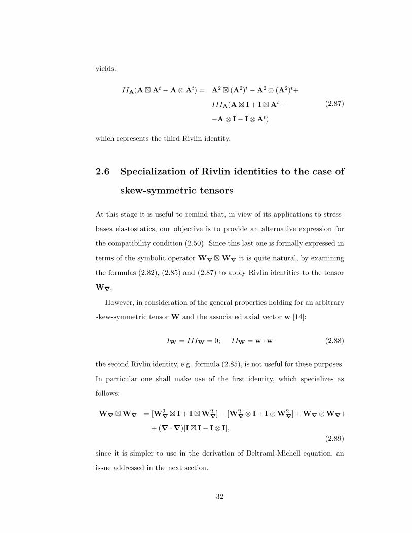
2.6 Specialization of Rivlin identities to the case of

skew-symmetric tensors

At this stage it is useful to remind that, in view of its applications to stress-

bases elastostatics, our objective is to provide an alternative expression for

the compatibility condition (2.50). Since this last one is formally expressed in

terms of the symbolic operator W∇ W∇ it is quite natural, by examining

the formulas (2.82), (2.85) and (2.87) to apply Rivlin identities to the tensor

W∇.

However, in consideration of the general properties holding for an arbitrary

skew-symmetric tensor W and the associated axial vector w [14]:

IW = IIIW = 0; IIW = w ·w (2.88)

the second Rivlin identity, e.g. formula (2.85), is not useful for these purposes.

In particular one shall make use of the first identity, which specializes as

follows:

W∇ W∇ = [W2∇

I + I W2∇

]− [W2∇⊗ I + I⊗W2

∇] + W∇⊗W∇+

+ (∇ ·∇)[I I− I⊗ I],

(2.89)

since it is simpler to use in the derivation of Beltrami-Michell equation, an

issue addressed in the next section.

32

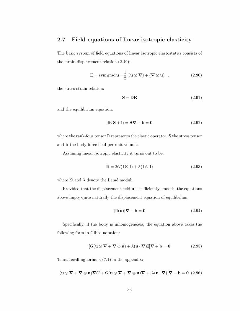
2.7 Field equations of linear isotropic elasticity

The basic system of field equations of linear isotropic elastostatics consists of

the strain-displacement relation (2.49):

E = sym gradu =1

2[(u⊗∇) + (∇⊗ u)] . (2.90)

the stress-strain relation:

S = DE (2.91)

and the equilibrium equation:

divS + b = S∇ + b = 0 (2.92)

where the rank-four tensor D represents the elastic operator, S the stress tensor

and b the body force field per unit volume.

Assuming linear isotropic elasticity it turns out to be:

D = 2G(I I) + λ(I⊗ I) (2.93)

where G and λ denote the Lame moduli.

Provided that the displacement field u is sufficiently smooth, the equations

above imply quite naturally the displacement equation of equilibrium:

[D(u)]∇ + b = 0 (2.94)

Specifically, if the body is inhomogeneous, the equation above takes the

following form in Gibbs notation:

[G(u⊗∇ + ∇⊗ u) + λ(u ·∇)I]∇ + b = 0 (2.95)

Thus, recalling formula (7.1) in the appendix:

(u⊗∇ + ∇⊗ u)∇G+G(u⊗∇ + ∇⊗ u)∇ + [λ(u ·∇)]∇ + b = 0 (2.96)

33

Applying formally the definition of tensor product to the second addend

and invoking formula (7.4) in the appendix for the third addend, one has:

(u⊗∇ + ∇⊗ u)∇G+G(∇ ·∇)u +G(u ·∇)∇+

+∇λ(u ·∇) + λ(u ·∇)∇ + b = 0

(2.97)

Upon rearranging, the displacement equation of equilibrium is finally arrived

at:

G∆u + (G+ λ)grad divu + [gradu + (gradu)t]gradG+

+(divu)gradλ+ b = 0

(2.98)

an expression which reduces to Navier’s equation in the case of homogeneous

bodies [29].

In particular, Navier’s equation is usually exploited [29, 56] to prove the

biharmonicity of the displacement field associated with divergence-free and

curl-free body force fields b together with additional properties concerning

divu, curlu, trE and trS.

As opposite to the straightforward and natural derivation of (2.98), the

basic equation of elastostatics expressed in terms of the stress tensor, known as

Beltrami-Michell equation or stress equation of compatibility, is considerably

more cumbersome to derive. It is classically obtained by exploiting properties

of the Ricci alternator, as in [38, 56, 36], or by using differential identities

which, though elegantly expressed in tensor form, are far from being intuitive

[29].

It is shown, on the contrary, that the proposed approach based on the use

of Rivlin identities, is considerably more constructive since it allows one to

derive Beltrami-Michell equation by purely algebraic manipulations in which

each step follows quite naturally from the previous ones.

34

2.8 Beltrami-Michell equation

To start with let us first invert the elasticity tensor (2.93) by writing:

D−1 =

1 + ν

E(I I)−

ν

E(I⊗ I) (2.99)

in terms of the Young modulus E and the Poisson ratio ν. Thus, the fun-

damental system of field equations governing the elastostatic problem of a

homogeneous linear isotropic body can also be written as:

S∇ + b = 0

E =[

1+υE I− υ

E (I⊗ I)]

S

(W∇ W∇)E = 0

equation of equilibrium

linear isotropic constitutive law

equation of compatibility

(2.100)

By substituting the second relation above in the third one:

1 + υ

E(W∇ W∇)S−

υ

E(W∇ W∇)(I⊗ I)S .

and invoking the composition rule (2.25)2 for the second addend:

(W∇ W∇)(I⊗ I) = W∇

Wt∇⊗I = −W2

∇⊗I (2.101)

the set of equations (2.100) becomes:

S∇ + b = 0

(W∇ W∇)S+υ

1 + υ(W2

∇⊗I)S = 0

equation of equilibrium

stress compatibility(2.102)

It is apparent that, in order to derive a unique formula expressed in terms of

the stress tensor, one needs to provide alternative expressions for the symbolic

tensors (W∇ W∇) and W2∇⊗ I which explicitly contain the term S∇

appearing in the equation of equilibrium.

In this respect we first invoke (2.16) to write:

W2∇ = ∇⊗∇− (∇ ·∇)I (2.103)

so that:

(W2∇⊗ I)S = (∇⊗∇)trS− (∇ ·∇)(trS)I (2.104)

35

The additional term (W∇ W∇)S which appears in (2.102) can be mod-

ified by invoking the specialization of the first Rivlin identity to the case of

skew-symmetric tensors see, e.g., formula (2.89). Thus, on account of (2.103)

one gets:

(W∇ W∇)S = (∇⊗∇)S + S(∇⊗∇)+

− 2(∇ ·∇)S− (∇⊗∇)trS+

− [(∇⊗∇) · S]I + 2(∇ ·∇)(trS)I+

+ (W∇ · S)W∇ + (∇ ·∇)S+

− (∇ ·∇)(trS)I

(2.105)

where the definition of dyadic and square tensor product between second-order

tensors has been exploited see, e.g., (2.22) and (2.23).

Observe that the quantity W∇ · S vanishes owing to the skew-symmetry

of W∇ and the symmetry of S so that, by invoking the properties (2.1) and

(2.2), the previous expressions become:

(W∇ W∇)S = ∇⊗ S∇ + S∇⊗∇− (∇ ·∇)S+

− (∇⊗∇)trS − (∇ · S∇)I+

+ (∇ ·∇)(trS)I

(2.106)

Thus, recalling (2.104), the stress compatibility condition (2.102)2 assumes

the form:

∇⊗ S∇ + S∇⊗∇−1

1 + ν(∇⊗∇)(trS)+

−(∇ ·∇)S +1

1 + ν(∇ ·∇)(trS)I− (S∇ ·∇)I = 0

(2.107)

The previous expression contains the terms (∇⊗S∇), (S∇⊗∇) and (∇·S∇).

Since the trace of the formers coincides with the latter it is natural to evaluate

the trace of the previous relation, to obtain the identity:

(∇ ·∇)(trS) =1 + ν

1− ν(S∇ ·∇). (2.108)

36

Substituting the previous expression in (2.107) provides:

∇⊗ S∇ + S∇⊗∇−1

1 + ν(∇⊗∇)(trS)+

−(∇ ·∇)S +ν

1− ν(S∇ ·∇)I = 0

(2.109)

which, on account of the equation of equilibrium (2.100)1 yields finally:

∆S +1

1 + ν(∇⊗∇)(trS) + b⊗∇ + ∇⊗ b +

ν

1− ν(b ·∇)I = 0 (2.110)

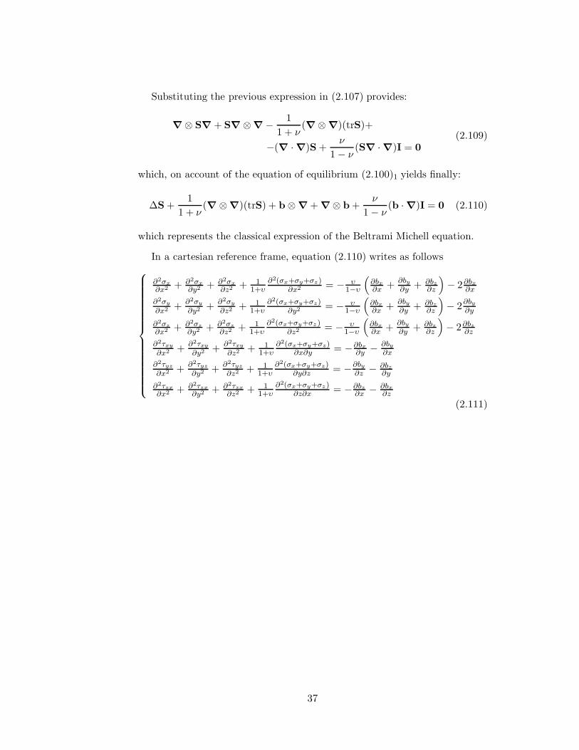
which represents the classical expression of the Beltrami Michell equation.

In a cartesian reference frame, equation (2.110) writes as follows

∂2σx

∂x2 + ∂2σx

∂y2 + ∂2σx

∂z2 + 11+υ

∂2(σx+σy+σz )∂x2 = − υ

1−υ

(

∂bx

∂x +∂by

∂y + ∂bz

∂z

)

− 2∂bx

∂x

∂2σy

∂x2 +∂2σy

∂y2 +∂2σy

∂z2 + 11+υ

∂2(σx+σy+σz)∂y2 = − υ

1−υ

(

∂bx

∂x +∂by

∂y + ∂bz

∂z

)

− 2∂by

∂y

∂2σz

∂x2 + ∂2σz

∂y2 + ∂2σz

∂z2 + 11+υ

∂2(σx+σy+σz )∂z2 = − υ

1−υ

(

∂bx

∂x +∂by

∂y + ∂bz

∂z

)

− 2∂bz

∂z

∂2τxy

∂x2 +∂2τxy

∂y2 +∂2τxy

∂z2 + 11+υ

∂2(σx+σy+σz)∂x∂y = −∂bx

∂y −∂by

∂x

∂2τyz

∂x2 +∂2τyz

∂y2 +∂2τyz

∂z2 + 11+υ

∂2(σx+σy+σz)∂y∂z = −

∂by

∂z −∂bz

∂y

∂2τzx

∂x2 + ∂2τzx

∂y2 + ∂2τzx

∂z2 + 11+υ

∂2(σx+σy+σz )∂z∂x = −∂bz

∂x −∂bx

∂z

(2.111)

37

38

Chapter 3

Saint Venant problem

The strategies for the general direct solution of Saint-Venant model for cylin-

ders with arbitrary cross section can be basically classified into two categories

known as displacement approach and stress approach according to the selected

unknown primary field and to the corresponding governing equations.

For what concerns the displacements approach [36], based on Cauchy-

Navier equations, the general solution was provided in the original work by

Barre De Saint-Venant [4] and by Alfred Clebsch [17] while a stress-based gen-

eral solution of Saint-Venant rod theory was presented by Riccardo Baldacci

[7] more than a century after the original paper by Barre De Saint-Venant.

Although the research is currently focused on Saint-Venant-like models en-

riched by additional complexity factors with respect to the classical problem

[10, 12], some basic issues of the homogeneous isotropic model are still object

of study and debate in the scientific community. These are concerned, in par-

ticular, on the solution of the shear problem and on the proper definition of

shear factors [54, 27, 44, 45], giving rise to very recent contributions as well

[35, 22].

As well known, regardless of the selected approach, the complete solution

in terms of displacements and stress fields for rods of generic cross section can

39

be represented by means of explicit analytic expressions only partially. Actu-

ally some terms associated with torsion and shear embody auxiliary functions

which are solution of Dirichlet or Neumann problems related to the cross

section domain; this is true with the exception of sections having particular

geometries for which a closed-form solution exists.

With special reference to the shear problem a further difference distin-

guishes the solutions available for this load case from the ones concerning ax-

ial load, biaxial bending and torsion. In these last cases, a frame-independent

representation for the displacement and the stress field is still available since

geometrical quantities which the solution depends upon are solely expressed

by means of vector and tensor fields.

For instance, it is well known that for bending and axial load the integral

quantities that characterize the dependence of the solution on the section

geometry are the first area moment and the inertia tensor. These quantities

in turn are defined as domain integrals extended over the section of the position

vector and of its tensor product. Actually, as illustrated in section 7.3 of the

appendix, the second order tensor associated with the matrix introduced by

Baldacci in [6, 7] changes as function of the adopted reference frame.

3.1 Saint Venant hypothesis

As well known Saint-Venant rod theory refers to a linearly elastic isotropic

cylinder of length l and cross section domain Ω.

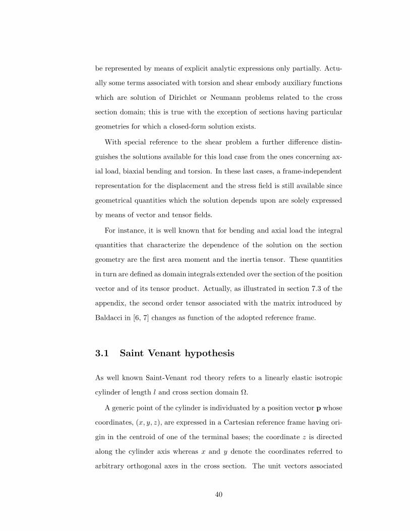
A generic point of the cylinder is individuated by a position vector p whose

coordinates, (x, y, z), are expressed in a Cartesian reference frame having ori-

gin in the centroid of one of the terminal bases; the coordinate z is directed

along the cylinder axis whereas x and y denote the coordinates referred to

arbitrary orthogonal axes in the cross section. The unit vectors associated

40

with the coordinate axes will be denoted by i, j, k, respectively.

x

y

z

z

i

k

j

τzx

σz

τzy

Since some properties of the section such as the inertia tensor are defined in

the cross-section, it is useful to introduce the vector

r = p − (p · k)k

which represents the projection of the position vector in the cross plane.

[r] =

x

y

0

Let us consider that the body-forces b and forces per unit area q on the

lateral surface Ωl are equals to zero:

b = 0 ∀p ∈ Ω

q = 0 ∀p ∈ ∂Ωl

(3.1)

It is also assumed a plane stress state:

σx = σy = τxy = 0 (3.2)

41

3.2 Stress field in the Saint-Venant theory

Differently from the classical contributions to the Saint-Venant problem, mainly

based on the displacement approach, in this work it will be referred to Bal-

dacci’s treatment. This author proposed an elegant and concise solution based

on a stress approach which, as such, takes its steps from Beltrami-Michell

equations [9, 40].

It is possible to derive some preliminary information on the stress field by

substitution of (3.2) in (2.111). In fact, in the light of (3.2) one has

xx)∂2(σx + σy + σz)

∂x2=∂2σz

∂x2= 0

yy)∂2(σx + σy + σz)

∂y2=∂2σz

∂y2= 0

xy)∂2(σx + σy + σz)

∂x∂y=∂2σz

∂x∂y= 0

zz)∂2σz

∂x2+∂2σz

∂y2+∂2σz

∂z2+

1

1 + ν

∂2σz

∂z2=

2 + ν

1 + ν

∂2σz

∂z2= 0

(3.3)

By the first three equations of (3.3) one observes that σz is a linear function

in x and y, so that the fourth one entails that σz is also a linear function in z:

σz = a0 + g · r + (l−z)(b0 + gt·r) (3.4)

where a0, b0,

g =

∣

∣

∣

∣

∣

∣

∣

∣

∣

∣

gx

gy

0

∣

∣

∣

∣

∣

∣

∣

∣

∣

∣

gt =

∣

∣

∣

∣

∣

∣

∣

∣

∣

∣

gtx

gty

0

∣

∣

∣

∣

∣

∣

∣

∣

∣

∣

constitute a set of six unknowns scalars to be evaluated as function of the

stress resultants applied on the end sections of the beam.

42

Substituting (3.2) in the equilibrium equation (2.92) provides:

∂σx

∂x+∂τxy

∂y+∂τxz

∂z=∂τxz

∂z= 0

∂τyx

∂x+∂σy

∂y+∂τyz

∂z=∂τyz

∂z= 0

∂τzx

∂x+∂τzy

∂y+∂σz

∂z= 0

(3.5)

the first two equations of (3.5) imply that τzx and τzy are independent of z,

while the third one is written as

div τ = ∇ · τ = −∂σz

∂z(3.6)

where τ is the vector parallel to xy plane whose component are:

τ =

∣

∣

∣

∣

∣

∣

∣

∣

∣

∣

τzx

τzy

0

∣

∣

∣

∣

∣

∣

∣

∣

∣

∣

On account of (3.5)1 and (3.5)2, the other two compatibility equations of

(2.111) become

xz)∂2τzx

∂x2+∂2τzx

∂y2+∂2τzx

∂z2+

1

1 + ν

∂2σz

∂z∂x=∂2τzx

∂x2+∂2τzx

∂y2+

1

1 + ν

∂2σz

∂z∂x= 0

yz)∂2τzy

∂x2+∂2τzy

∂y2+∂2τzy

∂z2+

1

1 + ν

∂2σz

∂z∂y=∂2τzy

∂x2+∂2τzy

∂y2+

1

1 + ν

∂2σz

∂z∂y= 0 .

(3.7)

In a vectorial form equations (3.7) can be equivalently expressed as

div gradτ = −1

1 + νgradσ′ , (3.8)

where σ′ =∂σz

∂z.

Moreover, by deriving (3.4) with respect by z one gets the following com-

patibility equation:

σ′ = (−b0 + gt · r)⇒ gradσ′ = −gt (3.9)

43

Thus, substitution of (3.9) in (3.8) yields

div gradτ =1

1 + νgt .

The scalar constant b0 in (3.4) turns out to be zero if the coordinate system

is barycentric. In fact, accordingly to Gauss’ theorem and (3.1)2 hypothesis

∫

∂A

τ · n ds = 0⇒

∫

A

div τ da = 0 (3.10)

since the substitution of (3.6) and (3.9) in (3.10) yelds

∫

A

(b0 + gt·r) da = 0 (3.11)

the scalar constant b0 is null being also null the first moment of inertia of the

section respect on the centroid:

∫

A

r da = 0 .

Resuming, the stress field solution of the Saint Venant problem in a barycen-

tric coordinate system is provided by a scalar component σz and a vector τ

fulfilling the following properties

σz = a0 + g · r + (l − z)gt·r

div τ = gt·r

div gradτ =1

1 + νgt

compatibility

equilibrium

compatibility

(3.12)

and τ · n = 0 on the boundary of the section.

Now it will be shown how an appropriate combination of the compatibility

equation with the equilibrium equation allows one to rewrite (3.12) in a more

convenient form.

div τ = gt·r

div gradτ = 11+ν gt

⇒

grad divτ = gt

div gradτ = 11+ν gt

. (3.13)

44

Subtracting the two equation in (3.13) one obtains

grad divτ−div gradτ =

(

1−1

1 + ν

)

gt =ν

1 + νgt = νgt. (3.14)

Invoking the triple vector product, see e.g.,

(∇ · τ )∇− (τ⊗∇)∇ = (∇ · τ )∇− (∇ ·∇)τ = ∇× (∇× τ ) = curl curl τ

that is

grad divτ−div grad τ = curl curl τ , (3.15)

so that equation (3.14) can be equivalently written as

curl curl τ = νgt (3.16)

Due to properties (3.5)1 and (3.5)2 curl τ is parallel to k, so that one has:

curl τ =∇× τ = (k⊗ k)∇× τ = (∇× τ · k)k . (3.17)

Accordingly, it turns out to be

curl curl r = ∇× (∇× τ ) = ∇× [(∇× τ · k)k] =

= −k× (∇× τ · k)∇ = Wtkgrad (curl τ · k)

(3.18)

substituting the previous relation (3.18) in (3.14) one has

Wtkgrad (curl τ · k) = νgt =⇒ curl τ · k = ν(Wkgt · r) + c.

where c is an arbitrary scalar

In conclusion, the stress vector τ solution of the Saint Venant problem can

be turned out by resolving the following linear differential problem:

div τ = τ ·∇ = gt·r

(curl τ )z = (∇× τ ) · k = νWkgt · r + c

equilibrium

compatibility(3.19)

with boundary conditions

τ · n = 0. (3.20)

45

expressing the condition of stress-free lateral surface.

The linearity of the previous problem naturally prompts for a staggered

solution scheme depending on the fact that gt is equal to or different from

zero. In order to separate the solution of the tangential stress field into shear

and torsion stress, the previous system can be written as the sum of the two

following systems:

τ tor ·∇ = 0

(∇× τ tor) · k = c

τ sh ·∇ = gt · r

(∇× τ sh) · k = νWkgt · r(3.21)

The solution of the relevant differential problems have been suffixed by

‘tor ’ and ‘sh’ to emphasize the fact that they are associated, respectively,

with torque or shear. In particular it will be show in this last case that gt is

directly associated with the shearing force ts

3.3 Stress field associated with torsion

The solution of the differential problem (3.21)1 is further decomposed in the

form

τ tor = τ 0tor + τp

tor (3.22)

where τ 0tor is the solution to the homogeneous system

τ 0tor ·∇ = 0

(∇× τ 0tor) · k = 0

(3.23)

whereas τptor is a particular integral

τptor ·∇ = 0

(∇× τ ptor) · k = c

(3.24)

To solve (3.24) the two equations are written in a more convenient form:

τptor·∇ = Wk(Wt

kτptor)·∇ = k× (Wt

kτptor)·∇ = −∇×(W t

kτptor)·k = −curl (Wt

kτptor)·k

46

∇× τ ptor · k = τ

ptor × k ·∇ = (Wt

kτptor) ·∇

thus, one obtains

curl (Wtkτ

ptor) · k = 0

(Wtkτ

ptor) ·∇ = c .

(3.25)

From the second equation in (3.25) it turns out to be

(Wtkτ

ptor) =

c

2r ⇒ τ

ptor =

c

2Wkr (3.26)

The solution of system (3.23) is a scalar harmonic function ϕtor so that

τ 0tor =

c

2grad ϕtor =

c

2ϕtor∇ (3.27)

The solution to the homogeneous differential problem (3.23) amounts to find-

ing a harmonic potential ϕtor, hence satisfying the condition (∇ ·∇)tor = 0,

with prescribed directional derivative along the boundary ∂Ω. Being

τ 0tor · n = −τ p

tor · n (3.28)

on account of (3.23) and (??), the homogeneous differential problem can be

equivalently formulated in the form

(∇ ·∇)ϕtor = 0 in the interior of Ω

(ϕtor ⊗∇)n = −c

2Wkr on the boundary ∂Ω

(3.29)

Hence on account of (3.27) and (3.26), (3.22) became

τ tor =c

2ϕtor∇ +

c

2Wkr (3.30)

in which τ tor represents the term of tangential stress associated with torsion.

3.4 Frame-independent representation of the stress

field associated with pure shear

Similarly to the previous section, the solution of differential problem (3.21)2

is additively decomposed in the form

τ sh = τ 0sh + τ p

sh (3.31)

47

where τ 0sh is the solution to the homogeneous system associated with (3.21)2

τ 0sh ·∇ = 0

(∇× τ 0sh) · k = 0

(3.32)

whereas τpsh is a particular integral of the non-homogeneous problem

τpsh ·∇ = gt · r

(∇× τpsh) · k = νWkgt · r

(3.33)

System (3.21)2 is supplemented by the boundary equation on ∂Ω

τ sh · n = 0. (3.34)

expressing the condition of stress-free lateral surface.

To obtain a frame-independent expression of τ psh it is set

τpsh = Apgt (3.35)

where

Ap = [α(r⊗ r) + β(r · r)I] (3.36)

whereas α and β are algebraic constants to be determined so as to fulfill (3.33)

and I is defined as

I = I− k⊗ k (3.37)

Substituting (3.35) in (3.33) and computing the divergence and the curl

of the monomials appearing in the expression (3.36) of Ap by means of the

formulas

(r⊗ r)gt ·∇ = gt · (r⊗ r)∇ = gt[r(r ·∇) + (r⊗∇)r] =

= gt(2r + r) = 3gt · r

(r · r)gt ·∇ = gt · (r · r)∇ = 2gt · r

[(r⊗ r)gt]×∇ · k = [(r · gt)r×∇] · k = k× r · gt = gt · r⊥

[(r · r)gt]×∇ · k = gt × 2r · k = −2k× r · gt = −2gt · r⊥

(3.38)

48

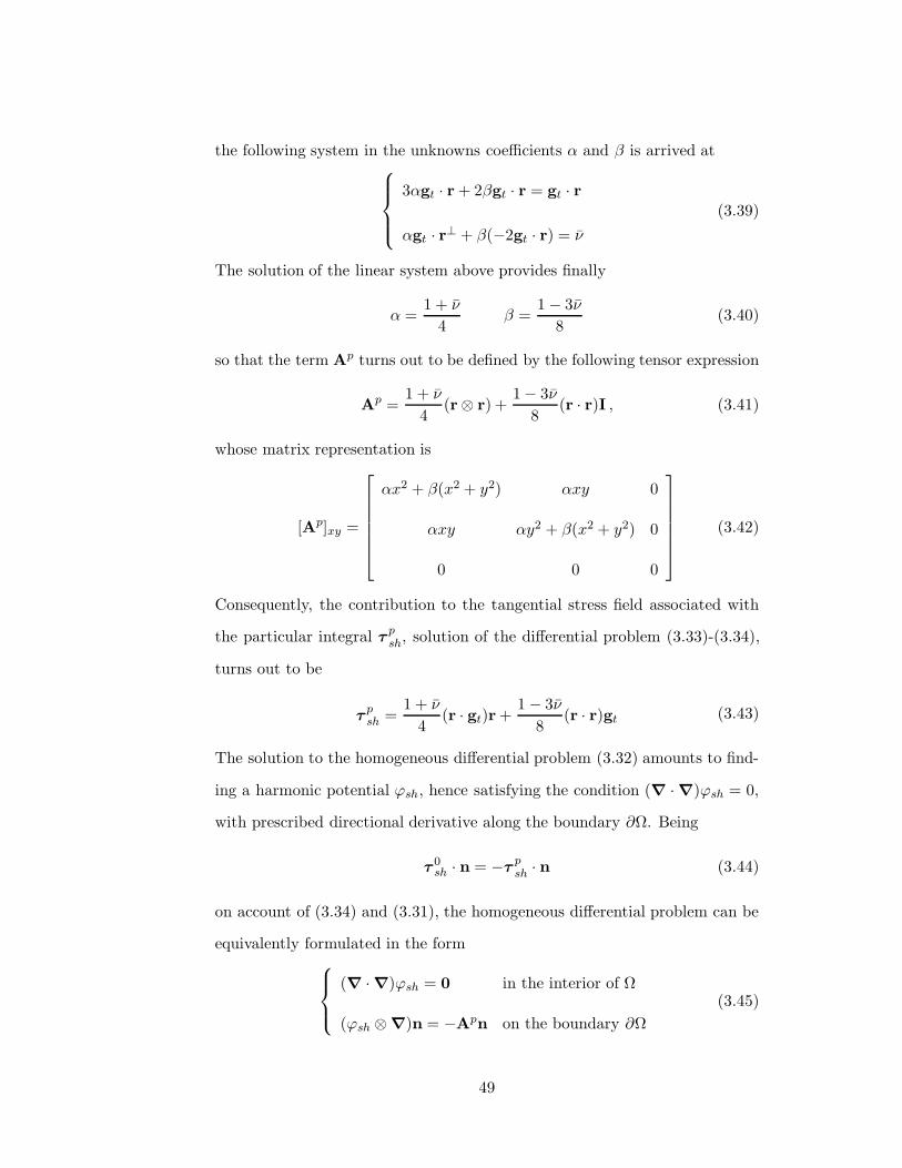
the following system in the unknowns coefficients α and β is arrived at

3αgt · r + 2βgt · r = gt · r

αgt · r⊥ + β(−2gt · r) = ν

(3.39)

The solution of the linear system above provides finally

α =1 + ν

4β =

1− 3ν

8(3.40)

so that the term Ap turns out to be defined by the following tensor expression

Ap =1 + ν

4(r⊗ r) +

1− 3ν

8(r · r)I , (3.41)

whose matrix representation is

[Ap]xy =

αx2 + β(x2 + y2) αxy 0

αxy αy2 + β(x2 + y2) 0

0 0 0

(3.42)

Consequently, the contribution to the tangential stress field associated with

the particular integral τ psh, solution of the differential problem (3.33)-(3.34),

turns out to be

τpsh =

1 + ν

4(r · gt)r +

1− 3ν

8(r · r)gt (3.43)

The solution to the homogeneous differential problem (3.32) amounts to find-

ing a harmonic potential ϕsh, hence satisfying the condition (∇ ·∇)ϕsh = 0,

with prescribed directional derivative along the boundary ∂Ω. Being

τ 0sh · n = −τ p

sh · n (3.44)

on account of (3.34) and (3.31), the homogeneous differential problem can be

equivalently formulated in the form

(∇ ·∇)ϕsh = 0 in the interior of Ω

(ϕsh ⊗∇)n = −Apn on the boundary ∂Ω

(3.45)

49

Let us observe that due to the special form of the boundary term, the potential

ϕsh depends on gt, and hence on the applied shear t so that this field does not

have a pure geometrical nature, as it happens for the quantities ϕtor, Ap and

JG, associated with pure torsion, bending and axial load, respectively, which

depend solely on the geometry of Ω.

For this reason, to state a problem equivalent to (3.45) exploiting a field

that has an exclusively geometrical nature one set

ϕsh = ψ · gt (3.46)

where the harmonic nature of ϕsh is carried over to ψ, (∇ ·∇)ψ = 0. By

virtue of (3.46) the boundary condition (3.45)2 can be written as

[(ψ · gt)∇] · n = −Apgt · n

(∇⊗ψ)gt · n = −gt · (Ap)tn

gt · (ψ ⊗∇)n = −gt · (Ap)tn

(3.47)

finally one obtains

gt ·[

(ψ ⊗∇)n + (Ap)tn]

= 0 (3.48)

Since the previous expression holds for any gt, the term under square brackets

must be zero and the boundary condition (3.45)2 can be equivalently expressed

as

(ψ ⊗∇)n = −(Ap)tn = −

[

1− ν

4(r⊗ r) +

1 + 3ν

8(r · r)I

]

n (3.49)

To sum up the harmonic vector field ψ is defined, up to a constant vector, as

the solution of the following Neumann vector problem

(∇ ·∇)ψ = 0 in the interior of Ω

(ψ ⊗∇)n = −Apn on the boundary ∂Ω

(3.50)

The tangential stress field associated with the shear force t is given by

τ sh = (∇⊗ψ) gt + Ap (r)gt (3.51)

50

3.5 Tangential stress field

The solution to differential system (3.21) is obtained by summing (3.30) and

(3.51)

τ = τ tor + τ sh = (∇⊗ψ)gt + Ap (r)gt +c

2ϕtor∇ +

c

2Wkr =

= [∇⊗ψ + Ap (r)]gt +c

2(ϕtor∇ + Wkr)

(3.52)

Notice from the previous formula that the tangential stress field τ is defined

only by purely geometrical entities

3.6 De Saint Venant stress field expressed in terms

of internal forces

Combining first equation in (3.12) with (3.52) gives

σz = a0 + g · r + (l− z)gt·r

τ = [∇⊗ ψ + Ap (r)]gt +c

2(ϕtor∇ + Wkr)

(3.53)

Notice from (3.53) that the stress field depends on a0, gt, g, c. This section

illustrates relations between these constants and the internal forces in order

to obtain an expression of the stress field that depends on these parameters.

Equilibrium equation to translation with respect to z direction gives

Nk =

∫

Aσ da =

∫

Aσk da =

=

[

a0

∫

Ada + g·

∫

Ar da + (l− z)gt·

∫

Ar da

]

k = a0Ak

thus

a0 =N

A(3.54)

while, equilibrium equation to translation in the plane x, y is expressed by

ts =

∫

Aτ da (3.55)

51

In order to develop integral in (3.55) on the boundary it is illustrated the

following property

(r⊗ τ )∇ = (r ·∇)τ + (τ ·∇)r = τ + (τ ·∇)r (3.56)

that can be simply verified by writing in indicial form

(riτj),j = ri,j τj + riτj,j = δijτj + riτj,j = τi + riτj,j

thus, in the light of (3.56), equation (3.55) become

ts =

∫

Adiv (r⊗ τ ) da −

∫

Ar(div τ ) da =

=

∫

∂A(r⊗ τ )n ds −

∫

Ar(gt·r) da =

=

∫

∂A

(τ · n)r ds−

∫

A

(r⊗ r)gt da

(3.57)

The first integral is equal to zero according to boundary condition τ · n = 0,

hence from (3.57) one has

ts = −JGgt ⇐⇒ gt = −J−1G ts . (3.58)

Equilibrium to rotation with respect to x and y axes gives

mf(z) =

∫

A

r× σzk da =

∫

A

r× (a0 + g · r + (l − z)gt·r)kda =

= a0

∫

A

r da × k +

∫

A

r× (g · r)k da + (l− z)

∫

A

r× (gt·r)k da =

= −k×

(∫

A(g · r)r da + (l− z)

∫

A(gt · r)rda

)

=

= Wtk

(∫

A

r⊗ r da

)

[g + (l− z)gt] =

= Wtk (JGg + (l− z)JGgt) = Wt

k (JGg − (l− z)ts)

(3.59)

hence

mf(z) = Wtk (JGg − (l− z)ts) ;

52

having set

mf(l) = ml

one has

ml = WtkJGg⇔ g = J−1

G Wkml ,

mf(z) = ml + (l− z)Wkts .

Moreover equilibrium to rotation with respect to z axis gives

mt =

∫

A

r× τ da =

(∫

A

Wkr · τ da

)

k (3.60)

by observing that both r and τ are orthogonal with respect to k

r× τ = (k⊗ k)(r× τ ) = (r× τ · k)k = (k× r · τ )k = (Wkr · τ )k (3.61)

thus, by substituting (3.61) in (3.60) it results

mt = Mtk . (3.62)

Finally, the stress field that satisfy De Saint Venant hypothesis in function

of the internal forces has the following expression:

σz =N

A+ J−1

G Wkml·r− (l−z)(J−1G ts·r)

τ = [∇⊗ψ + Ap (r)]J−1G +

c

2(ϕtor∇ + Wkr)

(3.63)

where ψ and ϕtor are harmonic functions that satisfy the boundary condi-

tions

(ϕtor ⊗∇)n = −c

2Wkr

(ψ ⊗∇)n = −Apn

(3.64)

3.6.1 The torsional stiffness factor

By setting

B(r) = ∇⊗ψ + Ap

53

in (3.52), one can obtain an alternative expression of mt:

mt =

[∫

AWkr ·B(r)gt da + c

2

∫

AWkr · (gradϕt + Wkr) da

]

k =

=

[

gt ·

∫

A

Bt(r)Wkr da + c2

∫

A

Wkr · (gradϕt + Wkr) da

]

k .

(3.65)

In the specific case of pure torsion (ts = 0)

gt = −J−1G t = 0 (3.66)

then, by (3.65) and (3.66)

mt =

[∫

AWkr·

c

2(gradϕt + Wkr) da

]

k =

=c

2

[∫

A(gradϕt ·Wkr + r · r) da

]

k =c

2Iqk

(3.67)

having introduced

Iq =

[∫

A(gradϕt ·Wkr + r · r) da

]

that represent the torsional stiffness factor.

The relation between Iq and mt can be reached by combining (3.62) and

(3.67):

mt = Mtk =c

2Iqk⇒ c = 2

Mt

Iq.

3.7 Closed-form analytical solutions

This section reports the analytical solution to the shear problem (3.50) in

terms of tangential stresses, for some common sections for which a closed-

form solution is available: the circular section, the elliptic section and the

rectangular section in the case ν = 0

54

3.7.1 Circular section

The solution to the previously stated shear problem has a significantly syn-

thetic expression for the circular section. It can be easily verified that the field

ψ, solution of (3.50), associated with a section of radius R is:

ψ = −(α + β)R2r = −3 + 2ν

8(1 + ν)R2r (3.68)

Actually, being linear, it is also harmonic and satisfies (3.50)1. Moreover, its

gradient, ψ ⊗∇, turns out to be

ψ ⊗∇ = −3 + 2ν

8(1 + ν)R2I. (3.69)

and on the boundary one has

r = Rn (3.70)

since the origin of the reference frame is located in the centroid. Thus, upon

substituting the previous relation into (3.36) one obtains

Apn =3 + 2ν

8(1 + ν)R2r (3.71)

an expression which fulfills the boundary condition (3.50)2 as well.

3.7.2 Elliptic section

In the case of the elliptic section it is convenient to express the solution in the

reference frame of the principal axes. In such a frame, say xy, one has

ψx

ψy

= −1

2(1 + ν)

2(1 + ν)R2x + R2

y

3R2x +R2

y

0

02(1 + ν)R2

y + R2x

3R2y +R2

x

x

y

+

+1− 2ν

8(1 + ν)

R2y −R

2x

3R2x + R2

y

0

0R2

x − R2y

3R2y + R2

x

x3

3− xy2

y3

3− yx2

(3.72)

55

where Rx and Ry are the principal radii of the ellipse. It can be easily verified

that the components of (3.72) are harmonic functions, as its terms x, y, x3

3 −xy2

andy3

3− yx2 do all possess such feature and it is also recognized that (3.72)

specializes to the matrix form of (3.68) whenever the axes have the same

length.

3.7.3 Rectangular section (ν = 0)

Provided that ν = 0, the present approach yields a closed form expression for

the harmonic vector potential ψ, and hence the shear stress τ sh analogous to

the classical solution reported in [57]. Observing that in this case the solution

is similar under several respects to the one for the elliptic section

[ψ] =

ψx

ψy

= −1

8

L2x 0

0 L2y

x

y

+1

8

x3

3− xy2

y3

3− yx2

(3.73)

where x and y are parallel to the edges of the rectangle whereas Lx and Ly are

their respective lengths. By virtue of (3.51) the shear stress field generated by

a shear force directed along y applied at the centroid turns out to be

τshx = 0, τshy =6tyLxL3

y

(

L2y

4− y2

)

(3.74)

56

Chapter 4

Displacement field, shear

center and deformability

tensor

This chapter illustrates the derivation of the displacement field associated

with each kind of internal force, e.g. axial force, biaxial bending, torsion and

biaxial shear. Moreover we provide the expression of the shear center and of

deformability tensor.

4.1 Derivation of the displacement field

As detailed in the introduction aim of this section is to complete the stress-

based solution of Saint-Venant problem due to Baldacci [6] by deriving the

displacement field separately for axial force, biaxial bending, torsion and bi-

axial shear.

57

4.1.1 Displacement field associated with axial force

By substituting g = gt = 0 in (3.4) one obtains the stress field associated with

axial force.

σz = a0 (4.1)

Hence the relevant stress tensor has the following expression

S =a0(k⊗ k) . (4.2)

Upon substituting the previous expression in the elastic-law (2.100)2 one gets

E =a0(1 + ν)

E(k⊗ k)−

a0ν

EI . (4.3)

The displacements field u associated with the stress field defined above can

be computed by means of a direct integration procedure which is substan-

tially equivalent to the use of Cesaro’s formulas [16]. In particular, once the

infinitesimal strain field E has been obtained, one can exploit the identity [29]

ω ⊗∇ = ∇×Et (4.4)

between the gradient of the axial vector ω of the skew-symmetric part of the

displacement gradient W and the curl of E. Thus, by employing the definition

(2.6), one can derive W as the cross product between ω and I, i.e. W = ω×I.

Finally, a second integration of the displacement gradient field u⊗∇ = E+W

provides the displacement field u which is looked for.

Since E is constant, it turns out to be

rotE = ∇×a0

E[(1 + ν)(k⊗ k)− νI] = 0

and

gradω = ω ⊗∇ = 0 =⇒ ω = ω0

the final result is

W = ω0 × I .

58

Apart from a rigid rotation, the gradient of displacement is symmetric so that

coincides with the strain tensor, i.e.

gradu = E =a0(1 + ν)

E(k⊗ k)−

a0ν

EI

Being constant integration of the previous relation provides

u =a0(1 + ν)

E(k⊗ k)p−

a0ν

Ep =

a0

E[(1 + ν)zk− νp] .

Upon substituting a0 = N/A an expression explicitly related to the normal

stress is obtained

u =N

EA(zk− νxi− νyj) .

4.1.2 Displacement field associated with biaxial bending

By substituting g = 0 and a0 = 0 in (3.4) one obtains the stress field due to

biaxial bending

σz = g · r (4.5)

Hence the stress tensor and the associated strain tensor have in turn the

following expressions

S =(g · r)(k⊗ k) . (4.6)

and

E =

[

1 + ν

EI−

ν

E(I⊗ I)

]

S =(1 + ν)

E(g · r)(k⊗ k)−

ν

E(g · r)I . (4.7)

The displacements field u associated with the stress field defined above can be

computed by means of a direct integration procedure which is substantially

equivalent to the use of Cesaro’s formulas [16]. In particular, starting from

(4.7) one can exploit the identity [29]

ω ⊗∇ = ∇× Et (4.8)

between the gradient of the axial vector ω of the skew-symmetric part of the

displacement gradient W and the curl of E.

59

Accordingly, by employing the definition (2.8), one can derive W as the

cross product between ω and I, i.e. W = ω× I. Finally, a second integration

of the displacement gradient field u⊗∇ = E + W provides the displacement

field u which is looked for.

Now it is necessary to compute curlE

curl E = ∇×1

E[(1 + υ)(g · r)(k⊗ k)− υ(g · r)I]t =

=(1 + υ)

E[∇× (g · r)k]⊗k−

υ

E[∇× (g · r)I]

by observing that

curl [(g · r)k] = ∇× (g · r)k = ∇(g · r)× k = grad (g · r)× k = g × k (4.9)

and

curl [(g · r)I] = ∇× (g · r)I = ∇(g · r)× I = grad (g · r)× I = g× I , (4.10)

one can express the gradient of ω and curl of E as follows

gradω = curlE =(1 + ν)

E[(g × k)⊗ k]−

ν

E(g × I) . (4.11)

Integration of constant tensors in (4.11) gives

ω =(1 + ν)

E[(g× k)⊗ k] r−

ν

E(g×r)+ω0 =

(1 + ν)

Ez(g×k)−

ν

E(g×r)+ω0

and then, except for a rigid rotation, the anti-symmetric part of grad u results

W = ω × I =(1 + ν)

Ez(g× k)× I−

ν

E(g × r)× I . (4.12)

On account of the following property

A× (b× c) = −(b× c)×A = (b⊗ c)A−(c⊗ b)A

the term on the left side of equation (4.12) can be expressed by

(g × k)× I = −I× (g × k) = (k⊗ g)−(g ⊗ k)

60

(g × r)× I = (r⊗ g)−(g ⊗ r)

hence, equation (4.12) becomes

W =(1 + ν)

Ez [(k⊗ g)−(g ⊗ k)]−

ν

E[(r⊗ g)−(g⊗ r)] .

Finally

gradu = E + W =

=(1 + ν)

E−(g⊗ zk) + k⊗ [(r · g)k + (r · k)g]+

ν

E(g⊗ r)− [(g · r)I+(r⊗ g)]

Integration of the previous formula is immediate by means of following expres-

sions

zk = gradz2

2=⇒ z(g ⊗ k) = grad

(

z2

2g

)

,

[(r·g)k+(r·k)g] = grad [(r·g)(r·k)] =⇒ k⊗[(r·g)k+(r·k)g] =grad [(r · g)(r · k)k] ,

r = grad|r|2

2=⇒ (g ⊗ r) = grad

[

(r · r)

2g

]

,

[(g · r)I+(r⊗ g)] = grad [(g · r)r] .

Finally, the displacement field associated with biaxial bending turns out to be

u =(1 + ν)

E

[

−z2

2g + z(r · g)k

]

+ν

E

[

(r · r)

2g − (g · r)r

]

+ω0 × r + u0 .

4.1.3 Displacement field associated with torsion

The tangential stress field τ tor is provided by (3.53) by setting gt = 0 so that

the stress tensor S becomes

S = (k⊗τ)+(τ⊗k) =[

k⊗c

2(gradϕt + Wkr)

]

+[ c

2(gradϕt + Wkr)⊗ k

]

.

(4.13)

Substituting the previous expression in the elastic-law (2.100)2 yelds

E =

[

1

2GI−

λ

2G(3λ+ 2G)(I⊗ I)

]

S (4.14)

61

Since the tensor S is traceless, it turns out to be

E =1

2G[(k⊗ τ ) + (τ ⊗ k)] =

c

2G

1

2[k⊗ (gradϕt + k× r)]+

1

2[(gradϕt + k× r)⊗k]

=

=c

2G

1

2[(gradϕt ⊗ k) + (k⊗ gradϕt)] +

1

2[(k× r)⊗ k] + [k⊗ (k× r)]

.

(4.15)

The displacements field u associated with torsion field is computed by follow-

ing the same steps outlined for biaxial bending; hence curl E is first evaluated.

curlE = ∇×1

2G[(k⊗ τ ) + (τ ⊗ k)] =

1

2G[(∇× k)⊗ τ ] + [(∇× τ )⊗ k] =

=1

2G− [k× (∇⊗ τ )] + [curl τ ⊗ k]

On account of (3.24)2, it turns out to be curl τ = ck, so that the previous

expression becomes

curlE =1

2G

[ck⊗ k]−[

k× (grad τ)t]

=

c

2G(k⊗ k)−

c

2G

k

2× [grad (gradϕt + k× r)]t

=

=c

2G

(k⊗ k)−1

2(k× I)

[

(grad gradϕt)t + (k× I)t

]

=

=c

2G

(k⊗ k)−1

2grad [(k× I)gradϕt] +

1

2(k× I)2

.

where in the last algebraic manipulation proper account has been made of

the fact that grad gradϕt is a symmetric tensor and k× I is skew-symmetric.

Finally

gradω =c

2G

(k⊗ k)−1

2grad [(k× I)gradϕt] +

1

2(k× I)2

.

Integration of the previous formula provides

ω =c

2G

[

zk−1

2(k× I)gradϕt +

1

2(k× I)2r

]

+ω0 (4.16)

in which ω0 is an arbitrary constant vector

62

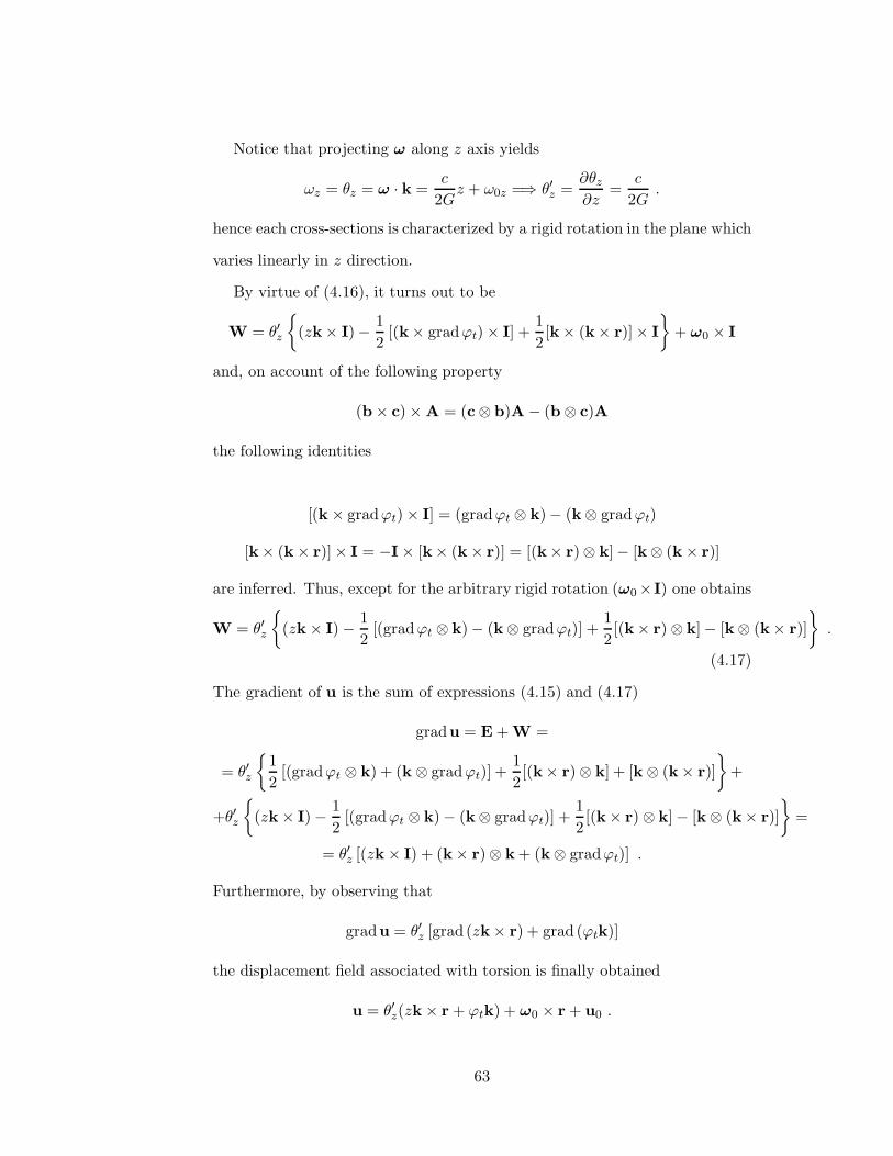
Notice that projecting ω along z axis yields

ωz = θz = ω · k =c

2Gz + ω0z =⇒ θ′z =

∂θz∂z

=c

2G.

hence each cross-sections is characterized by a rigid rotation in the plane which

varies linearly in z direction.

By virtue of (4.16), it turns out to be

W = θ′z

(zk× I)−1

2[(k× gradϕt)× I] +

1

2[k× (k× r)]× I

+ ω0 × I

and, on account of the following property

(b× c)×A = (c⊗ b)A− (b⊗ c)A

the following identities

[(k× gradϕt)× I] = (gradϕt ⊗ k)− (k⊗ gradϕt)

[k× (k× r)]× I = −I× [k× (k× r)] = [(k× r)⊗ k]− [k⊗ (k× r)]

are inferred. Thus, except for the arbitrary rigid rotation (ω0×I) one obtains

W = θ′z

(zk× I)−1

2[(gradϕt ⊗ k)− (k⊗ gradϕt)] +

1

2[(k× r)⊗ k]− [k⊗ (k× r)]

.

(4.17)

The gradient of u is the sum of expressions (4.15) and (4.17)

gradu = E + W =

= θ′z

1

2[(gradϕt ⊗ k) + (k⊗ gradϕt)] +

1

2[(k× r)⊗ k] + [k⊗ (k× r)]

+

+θ′z

(zk× I)−1

2[(gradϕt ⊗ k)− (k⊗ gradϕt)] +

1

2[(k× r)⊗ k]− [k⊗ (k× r)]

=

= θ′z [(zk× I) + (k× r)⊗ k + (k⊗ gradϕt)] .

Furthermore, by observing that

gradu = θ′z [grad (zk× r) + grad (ϕtk)]

the displacement field associated with torsion is finally obtained

u = θ′z(zk× r + ϕtk) + ω0 × r + u0 .

63

4.1.4 Displacement field associated with biaxial shear

The tangential stress field τ sh is provided by (3.51) so that the stress tensor

has the following expression

S = (l− z)(gt · r)(k⊗ k) + τ sh ⊗ k + k⊗ τ sh. (4.18)

We recall once more that the skew-symmetric part of the displacement gradient

W is obtained as the cross product between ω and I, i.e. W = ω × I, where

ω is obtained from

ω ⊗∇ = ∇×Et (4.19)

once the infinitesimal strain tensor E is derived from (4.19) via the linear elas-

tic law. In this way, being u ⊗∇ = E + W, a second integration provides

the displacement field u which is looked for. To simplify the integration pro-

cedure illustrated below, it is useful to express alternatively the shear stress

field (3.51) upon introducing the vector

a =1

8(r · r)r (4.20)

whose gradient is the symmetric tensor

a⊗∇ = ∇⊗ a =1

8[2(r⊗ r) + (r · r)I] (4.21)

The vector a allows one to express Ap in (3.41) as

Ap = (1 + ν)(∇⊗ a) − νr · r

2I (4.22)

so that the tangential stress field (3.51) becomes

τ sh = [(∇⊗ψ) + (1 + ν)(∇⊗ a)− νr · r

2I]gt (4.23)

The previous relation, upon introducing the vector ξ, defined as

ξ = ψ + (1 + ν)a (4.24)

64

becomes

τ sh =(

∇⊗ ξ − νr · r

2I)

gt = (ξ · gt)∇− νr · r

2gt. (4.25)

Applying the linear isotropic law

E =1 + ν

ES−

ν

E(tr S)I (4.26)

to (4.18), the following representation is obtained for the infinitesimal strain

field

E =1 + ν

E[(l− z)(gt·a)(k⊗ k) + (τ sh ⊗ k) + (k⊗ τ sh)]+

−ν

E[(l− z)(gt·a)I]

(4.27)

Substituting (4.25) into the previous expression and setting the relation

(1 + ν)ν = ν (4.28)

one finally obtains

E =1 + ν

E(l− z)(gt·a)(k⊗ k) + [(ξ · gt)∇]⊗ k + k⊗ [(ξ · gt)∇]+

−ν

E[(l− z)(gt·a)I +

r · r

2gt ⊗ k + k⊗

r · r

2gt]

(4.29)

The explicit computation of the curl of E, i.e. ∇ × Et, required by the pre-

viously outlined integration procedure, needs the separate computation of the

65

curl of the addends contained in the RHS of the previous expression

∇× [(l− z)(gt·a)(k⊗ k)] = (l− z)(gt·a)∇× (k⊗ k) =

= [(l−z)gt − (gt·a)k]×(k⊗ k) =

= (gt × k)⊗(l− z)k

∇× [k⊗ (ξ · gt)∇] = [∇× k]⊗(ξ · gt)∇ =

= − (k×∇)⊗(ξ · gt)∇ =

= −k× [∇⊗ (ξ · gt)∇] =

= −Wk [(ξ · gt)∇⊗∇]

∇× [(ξ · gt)∇⊗ k] = [∇× (ξ · gt)∇]⊗ k = 0

∇× [(l− z)(gt·a)I] = (l− z)(gt·a)∇× I =

= [(l− z)gt + (gt·a)k]×I =

= (l− z)Wgt+ (gt·a)W

k

∇

(

k⊗r · r

2gt

)

= −k×[

∇r · r

2⊗ gt

]

=

= −k× r⊗ gt

∇

[(r · r

2

)

gt ⊗ k]

=[

∇

(r · r

2

)]

× gt ⊗ k = r× gt ⊗ k

(4.30)

The identities above can be proven by invoking the differential identities re-

ported in the Appendix A. Using the identities (4.30) the curl of E becomes

∇×Et =1 + ν

E(gt×k)⊗ (l− z)k−k× [(ξ · gt)∇⊗∇]+

+ν

E−r× gt ⊗ k + k× r⊗ gt+

+ν

E[(z − l)gt × I + (gt · r)k× I]

(4.31)

On account of identity (4.19), one knows the expression of the gradient of ω;

hence, to obtain ω, it is necessary to integrate the expression above. To this

66

end (4.31) is further developed as follows

ω ⊗∇ =1 + ν

E

(

lz −z2

2

)

(gt × k)− k× [(ξ · gt)∇]

⊗∇+

+ν

E[gt × r⊗ k + k× r⊗ gt + (z − l)gt × I + (gt · r)k× I] =

=1 + ν

E

(

lz −z2

2

)

(gt × k)− k× [(ξ · gt)∇]

⊗∇+

+ν

E

[

(z − l)gt × I + (gt · r)k× r +z2

2(k× gt)

]

⊗∇

(4.32)

In particular, the last equality in (4.32) hinges on the identity

gt × r⊗ k + (z − l)gt × I = [(z − l)gt × p]⊗∇ +

[

z2

2(k× gt)

]

⊗∇ (4.33)

which is inferred from the relation r = p− zk.

The rightmost expression in (4.32) allows one to directly identify the ex-

pression of the axial vector ω

ω =1 + ν

E

(

lz −z2

2

)

(gt×k)−k×(ξ · gt)∇

+

+ν

E

[

(z − l)gt × p + (gt · p)k× p +z2

2(k× gt)

]

+ ω0

(4.34)

where ω0 is an arbitrary constant vector field. Accordingly, the skew-symmetric

component of the displacement gradient W, whose axial vector is ω, it turns

out to be:

W = ω × I =1 + ν

E

(

lz −z2

2

)

(gt × k)× I− [k× (ξ · gt)∇]× I

+

+ν

E

k×

[

(gt · p)p +z2

2gt

]

× +[gt × (z − l)p]× I

+ω0 × I,

The last addend ω0 × I is the displacement gradient of an arbitrary rigid

motion up to which the displacement solution is defined. For sake of brevity

this term will be omitted in the following developments although it will be

reported in the final expression of the displacements.

67

Recalling identity (2.17) one infers

W =1 + ν

E

(

lz −z2

2

)

[(k⊗ gt)− (gt ⊗ k)] + [k⊗ (ξ · gt)∇]− [(ξ · gt)∇⊗ k]

+

+ν

E

[

(gt · p)p +z2

2gt

]

⊗ k− k

[

(gt · p)p +z2

2gt

]

+

+ [(z − l)p⊗ gt]− [gt ⊗ (z − l)p]

(4.35)

By definition, the sum of the expression above with that of E reported in (4.29)

provides the displacement gradient grad u = u ⊗∇. Comparing expressions

(4.29) and (4.35) one recognizes the presence of two terms premultiplied either

by the coefficient 1+νE or by ν

E . For this reason, for the sake of readability the

following representation is exploited in the computation of the displacement

gradient. In particular, the integral of grad u1+ν can be achieved more easily

upon developing the integrand as follows

grad u1+ν = (l− z)(gt · r)(k⊗ k) + [(ξ · gt)∇⊗ k] + [k⊗ (ξ · gt)∇]+

+

(

lz −z2

2

)

(k⊗ gt)− (gt ⊗ k)] + [k⊗ (ξ · gt)∇]− [(ξ · gt)∇⊗ k]

=

=

(

lz −z2

2

)

(gt · p)k + 2(ξ · gt)k

(

z3

6− l

z2

2

)

gt

⊗∇

(4.36)

Following an analogous strategy for grad uν one has:

grad uν = (l− z)(gt · r)I−r · r

2gt ⊗ k− k⊗

r · r

2gt+

+

[

(gt · p)p +z2

2gt

]

⊗ k− k⊗

[

(gt · p)p +z2

2gt

]

=

+[(l− z)p⊗ gt]− [gt ⊗ (z − l)p] =

=

(z − l)(gt·p)p−

[

(z − l)(p · p)

2−z3

3

]

gt −(p · p)

2(gt·p)k

⊗∇

(4.37)

Finally, adding all displacement terms and including the integration constants

68

u0 and ω0 as well, the required displacement field turns out to be

u =1 + ν

E

(

lz −z2

2

)

(gt·p)k− 2(ξ · gt)k+

(

z3

6− l

z2

2

)

gt

+

+ν

E

(z − l)(gt·p)p−

[

(z − l)(p · p)

2−z3

3

]

gt −p · p

2(gt · p)k

+

+ω0 × p + u0

(4.38)

Upon substituting gt = −J−1G t an expression explicitly related to the shear

force is obtained

u =1 + ν

E

−

(

lz −z2

2

)

(J−1G t·p)k + 2(ξ · J−1

G t)k−

(

z3

6− l

z2

2

)

J−1G t

+

+ν

E

−(z − l)(J−1G t · p)p +

[

(z − l)(p · p)

2−z3

3

]

J−1G t+

+ (J−1G t · p)

(p · p)

2k

+ω0 × p + u0

Comparing (4.1.4) with the classic expression reported by [36], which addresses

a section loaded by a shear force directed along the x axis, one finds the

following relation (4.1.4)

ψx =1

2(1 + ν)

[

−χ− xy2 −1

4(r · r)x

]

(4.39)

between the function χ introduced by Love and the component along x of the

auxiliary function ξ appearing in the formula above. Actually,

ξx = ψx +1

8(1 + ν)(r · r)x (4.40)

by means of formulas (4.20) and (4.24).

4.2 Shear center

Aim of this section is to derive a frame-independent expression of the shear cen-

ter on account of the previously derived representation for tangential stresses

originated by pure shear (3.51).

69

The shear center ρC is defined as the point of the transverse cross plane

common to all lines of action of the resultants of the shear stress fields char-

acterized by zero torsional rotation, i.e. by

θ′ =Mt

Iq= 0. (4.41)

According to such definition, setting θ′ = 0 in (38)2, the tangential stress field

generated by pure shear τ sh, admits the following expression.

τ sh = − [Ap (r) + (∇⊗ψ)]J−1G t (4.42)

The shear center ρC must consequently fulfill the property

ρC × t · k =

∫

Ωr× τ shdA · k (4.43)

stating the static equivalence of the vector t applied at rC with the field τ sh.

Considering the identity

r× τ sh = (k⊗ k)(r× τ sh) = (r× τ sh · k)k = (r⊥ · τ sh)k (4.44)

one infers from (4.42) and (4.44)

(k×ρC)·t = r⊥C ·t = −

∫

Ω[Ap (r) + (∇⊗ ψ)]t r⊥·J−1

G t dA = −γ ·J−1G t (4.45)

where it has been set

γ = −

∫

Ω[Ap (r) + (∇⊗ ψ)]t r⊥ dA (4.46)

Notice that, recalling definition (3.41) for Ap and observing that (r⊗r)(k×r =

0), one can also write

γ = −

∫

Ω

[

(ψ ⊗∇) +1− 3ν

8(r · r)I

]

r⊥ dA (4.47)

Recalling that J−1G is symmetric, formula (4.35) becomes

k× rC · t = −J−1G γ · t (4.48)

70

and hence for the arbitrariness of t,

k× rC = −J−1G γ (4.49)

A vector premultiplication of both members by k yields

rC = k× (J−1G γ) , (4.50)

so that, invoking (4.46), one finally has

rC = k×

J−1G

∫

Ω

[

(ψ ⊗∇) +1− 3ν

8(r · r)I

]

(k× r)dA

. (4.51)

Observe that all terms in the previous expression are frame independent quan-

tities.

4.2.1 Boundary integral tensor expression of the shear center

We are going to illustrate the manipulations that provide a boundary integral

expression of the shear center by means of Gauss theorem. Since a formula of

this type is available for JG

JG =1

4

∫

∂Ω(r⊗ r)(r · n)dA , (4.52)

it is sufficient to develop a boundary form of the sole term given by (4.47).

Invoking the product rule, the first addend in (4.47) can be written as follows

(∇⊗ψ)r⊥ = (ψ ⊗ r⊥)∇− (r⊥ ·∇)ψ = (ψ ⊗ r⊥)∇ (4.53)

since r⊥ ·∇ = 0.

Similarly, the second integrand in (4.47), containing (r · r)r⊥, can be also

expressed as a boundary integral on account of the identity

[(r · r)]r⊥ = [(r · r)(r⊗ r⊥)]∇ (4.54)

71

which is proved in section 7.4 of the appendix. Thus, by virtue of the diver-

gence theorem, the integral (4.47) can be expressed as

γ =

∫

∂Ω

[

ψ ⊗ r⊥]

n dA+1− 3ν

8

∫

∂Ω

[(r · r)(r⊗ r⊥)]n dA =

=

∫

∂Ω

[

(r⊥ · n)ψ]

n dA+1− 3ν

8

∫

∂Ω

(r⊥ · n)(r · r)r dA .

(4.55)

Upon substituting finally (4.55) into (4.50), one obtains the required boundary

integral expression of the shear center

ρC = k×

J−1G

∫

∂A

[

(ψ +1− 3ν

8(r · r)I

]

(r⊥ · n) dA

. (4.56)

The previous expression turns out to be particularly useful in numerical com-

putations

4.2.2 Further developments for polygonal sections

Introducing the following parametric representation

r(µ) = rl + µ∆rl (4.57)

where

∆rl = rl+1 − rl (4.58)

the unit vector n normal to the boundary can be written

n =∆rl

ll× k = −

1

ll∆r⊥l . (4.59)

Substituting (4.57) and (4.59) in the terms (r · n) and (r ⊗ r) appearing in

(4.55) one has

r⊥ · n = (r⊥l + µ∆r⊥l )(−1

ll∆r⊥l ) = −

1

ll(r⊥l ·∆r⊥l )− llµ

r⊗ r = rl ⊗ rl + 2µ(rl ⊗∆rl) + µ2(∆rl ⊗∆rl) = T1 + 2µT2 + µ2T3

(4.60)

72

where

T1 = rl ⊗ rl

T2 = rl ⊗∆rl

T3 = ∆rl ⊗∆rl

(4.61)

Since

µ =s

ll⇒ dµ =

dA

ll, (4.62)

by (4.55), it turn out to be

−

nv∑

l=1

∫ 1

0[(r⊥l ·∆r⊥l ) + µl2l ](T1 + 2µT2 + µ2T3)(rl + µ∆rl)dµ =

= −

nv∑

l=1

(r⊥l ·∆r⊥l )T1rl +

∫ 1

0

[

(r⊥l ·∆r⊥l )(T1∆rlµ+ T2rlµ+

+T2∆rlµ2 + T3rlµ

2 + T3∆rlµ3) + l2l (T1rlµ+ T1∆rlµ

2+

T2rlµ2 + T2∆rlµ

3 + T3rlµ3 + T3∆rlµ

4)]

dµ =

= −

nv∑

l=1

[

(r⊥l ·∆r⊥l )T1rl +

∫ 1

0(s1µ+ s2µ

2 + s3µ3 + l2l T3∆rlµ

4)dµ

]

(4.63)

being

s1 = (r⊥l ·∆r⊥l )T1∆rl + (r⊥l ·∆r⊥l )T2rl + l2l T1rl

s2 = (r⊥l ·∆r⊥l )T2∆rl + (r⊥l ·∆r⊥l )T3rl + l2l T1∆rl + l2l T2rl

s3 = (r⊥l ·∆r⊥l )T3∆rl + l2l T2∆rl + l2l T3rl

(4.64)

4.3 Frame-independent form of the shear flexibility

tensor

According to the energetic definition [44, 49], the shear flexibility tensor is

defined as the tensor Ds such that the equivalence U shDs

= U sh is satisfied,

where U sh is the strain energy associated with shear

U sh =1

2G

∫

Ωτ sh · τ shdA (4.65)

73

whereas U shDs

is the elastic energy term expressed as the Ds-associated quadratic

form operating on the shear force vectors t

U shDs

=1

2Dst · t (4.66)

Such a definition provides

Ds =1

GJ−1

G ΦJ−1G (4.67)

where

Φ =

∫

Ω

(ψ ⊗∇+ Ap)(∇⊗ψ + Ap)dA (4.68)

Tensor Φ and the adimensional tensor of shear coefficients χ are related, see

e.g.

χ = AJ−1G ΦJ−1

G (4.69)

4.3.1 Expression of the shear flexibility tensor by means of

boundary integrals

This section illustrates a procedure for transforming the domain integral (4.68)

in a complete boundary form exploiting the divergence theorem. For the sake

of clarity, an indicial notation is used in some of the developments reported

below. Integral (4.68) turns out to be the sum of four terms

Φ =

∫

Ω[(ψ ⊗∇)(∇⊗ ψ) + (ψ ⊗∇)Ap + Ap(∇⊗ ψ) + ApAp]dA. (4.70)

and in indicial notation reads

Φij=

∫

Ω[Ap

ik(ψj, k +Apkj) + ψi, kψj, k + ψi, kA

pkj]dA (4.71)

In order to achieve a boundary integral expression of (4.71), the following

identity

Φij=

∫

Ω

[

1

2(Ap

ikψj + Apjkψi) ,k − (ψjρi + ψiρj) + Ap

ikApkj

]

dA (4.72)

74

will be preliminarily derived.

Since ψ is harmonic, ψj, kk = 0, one infers from the product rule

ψi, kψj, k = (ψiψj, k), k − ψiψj, kk = (ψiψj, k), k (4.73)

and one also has

ψi, kApkj = (ψiA

pkj), k − ψiA

pkj, k (4.74)

Substituting (4.73) and (4.74), into (4.71) one obtains

Φij =

∫

Ω

(Apikψj, k +Ap

ikApkj − ψiA

pkj, k) dA+

∫

Ω

(ψiψj, k + ψiApkj), k dA (4.75)

It is recognized that the second integral above vanishes on account of the

divergence theorem; actually, invoking the symmetry of Ap in (3.41), such an

integral can be written as follows

∫

Ω

ψi(ψj, k +Apkj), k dA =

∫

∂Ω

(ψiψj, k + ψiApkj)nk ds = 0 (4.76)

where the last equality holds by virtue of the boundary constraint (3.50)2

(ψj, k +Apjk)nk = 0 (4.77)

Hence (4.71) reduces to

Φij =

∫

Ω

(Apikψj, k − ψiA

pkj, k + Ap

ikApkj) dA (4.78)

Upon observing that

Apikψj, k = (Ap

ikψj), k − Apik, kψj (4.79)

the integrand function of (4.78) can be further transformed as follows

Φij =

∫

Ω[(Ap

ikψj), k − Apik, kψj +Ap

ikApkj − ψiA

pkj, k] dA (4.80)

The previous expression can be further transformed in a form which more

clearly emphasizes the symmetry of Φ. Actually, by (4.77), one has

∫

Ω(Ap

ikψj), kdA =

∫

∂Ω(Ap

ikψj)nkds =

∫

∂Ω(−ψi, kψj)nkds =

∫

Ω(−ψi, kψj), k dA

(4.81)

75

while the harmonicity of ψ, ψj, kk = 0, yields

(−ψi, kψj), k = (−ψiψj, k), k (4.82)

From (4.81) and (4.82) one eventually infers

∫

Ω(Ap

ikψj), kdA =

∫

Ω(Ap

ikψi), kdA =

∫

Ω

1

2(Ap

ikψj +Apjkψi), k dA (4.83)

so that (4.80) is equivalent to

∫

Ω

[

1

2(A

pikψj + A

pjkψi), k − (A

pik ,kψj + ψiA

pkj ,k) +A

pikA

pkj

]

dA (4.84)

By taking the divergence of (3.41), which provides Apik, k = ρi, the second

integrand term in (4.84) can be further simplified to obtain the required result

(4.72). This preliminary result allows one to transform (4.72) in a boundary

integral. To this end it is necessary to transform the second and third integrand

terms of (4.72) into the divergence of a tensor, just as for the first term. For

greater clarity we introduce the notation

Φij = Φ(1)ij + Φ

(2)ij + Φ

(3)ij (4.85)

Φ(1)ij =

∫

Ω

1

2(A

pikψj + A

pjkψi), k dA (4.86)

Φ(2)ij = −

∫

Ω

ψjρi + ψiρj dA (4.87)

Φ(3)ij =

∫

ΩAp

ikApkj dA (4.88)

Considering the explicit expression (3.41) of Ap and the divergence theorem

one has for Φ(1)

Φ(1) =

∫

∂Ω

[

α

2(r · n)(r⊗ ψ + ψ ⊗ r) +

β

2(r · r)(n⊗ ψ +ψ ⊗ n)

]

ds (4.89)

76

Making use of p, previously introduced in (4.20), the integrand of (4.88) is

expressed as the divergence of a tensor

ψirj = ψipj, kk, ψjri = ψjpi, kk (4.90)

and on account of the property of being harmonic, which provides

ψipi, kk = (ψipi, k), k − (ψi, kpi), k

ψjpi, kk = (ψjpi, k), k − (ψj, kpi), k

(4.91)

Relation (4.90) is inferred on account of the following identity

ψj, kk = ρj (4.92)

which is proven in section 7.4.2 of the appendix.

Considering the further identity

pi, k =1

8(2ρkρi + ρhρhδik) (4.93)

which is proven as well in section 7.4.2 of the appendix, and relation (4.77),

the following boundary integral

Φ(2) =

∫

∂Ω

[

−1

4(r · n)(r⊗ ψ +ψ ⊗ r)−

1

8(r · r)(n⊗ψ + ψ ⊗ n)

]

ds +

+

∫

∂Ω

[

−2α

8(r · r)(r · n)(r⊗ r)−

β

8(r · r)2(r⊗ n + n⊗ r)

]

ds

(4.94)

is derived in tensor notation.

For what concerns the third addend Φ(3) of (4.86), it is necessary to express

in divergence form the integrand

ApAp = (α2 + 2αβ)(r · r)(r⊗ r) + β2(r · r)2I (4.95)

This is achieved by means of the following formulas

(ρiρi)ρhρk =1

6[(ρiρi)ρhρkρl], l

(ρpρp)(ρqρq) =1

6[(ρpρp)(ρqρq)ρl], l

(4.96)

77

that are proved in sections 7.4.3 and 7.4.4 of the appendix, respectively. Owing

to these formulas and to the divergence theorem one infers

Φ(3)ij =

∫

∂Ω

(α2 + 2αβ)

6[(ρiρi)ρhρk] +

β2

6[(ρprp)(ρqrq)δhk]

ds (4.97)

or, in implicit notation

Φ(3) =

∫

∂Ω

[

α2 + 2αβ

6(r · r)(r · n)(r⊗ r) +

β2

6(r · r)2(r · n)I

]

ds . (4.98)

Adding (4.89), (4.94), (4.98) and collecting the resulting terms the sought

entirely boundary expression of the shear flexibility tensor is obtained

Φ =

(

α

2−

1

4

)∫

∂Ω

(r · n)(r⊗ ψ +ψ ⊗ r) ds +

+

(

β

2−

1

8

)∫

∂Ω(r · r)(n⊗ψ +ψ ⊗ n) ds +

+

(

α2 + 2αβ

6−α

4

)∫

∂Ω(r · r)(r · n)(r⊗ r) ds +

−β

8

∫

∂Ω(r · r)2(r⊗ n + n⊗ r) ds +

+β2

6

∫

∂Ω

(r · r)2(r · n)I ds

(4.99)

Substituting (3.40) in the previous formula one finally obtains

Φ = −1− ν

8

∫

∂Ω(r · n)(r⊗ ψ + ψ ⊗ r) ds +

−1 + 3ν

16

∫

∂Ω

(r · r)(n⊗ ψ +ψ ⊗ n) ds +

−2 + 3ν + ν2

48

∫

∂Ω(r · r)(r · n)(r⊗ r) ds +

−1− 3ν

64

∫

∂Ω(r · r)2(r⊗ n + n⊗ r) ds +

+(3ν − 1)2

384

∫

∂Ω(r · r)2(r · n)I ds.

(4.100)

which can be substituted in (4.69) to get, invoking also (4.52), an expression

of the shear flexibility tensor expressed solely by means of boundary integrals.

78

4.3.2 Shear flexibility tensor for the circular section

The general expression of Φ presented in (4.100) can be specified to a circular

section of radius R by setting

r = Rn (4.101)

hence

Φ = +(3 + 2ν)

32(1 + ν)2R5

∫

∂Ω(n⊗ n) ds +

+(1 + 4ν)(3 + 2ν)

64(1 + ν)2R5

∫

∂Ω

(n⊗ n) ds +

−(2 + 7ν + 6ν2)

48(1 + ν)2R5

∫

∂Ω(n⊗ n) ds +

+2ν − 1

32(1 + ν)R5

∫

∂Ω(n⊗ n) ds +

+(2ν − 1)2

384(1 + ν)2R5

∫

∂ΩI ds. =

=13 + 32ν + 12ν2

192(1 + ν)2R5

∫

∂Ω

(n⊗ n) ds +

+(2ν − 1)2

384(1 + ν)2R5

∫

∂ΩI ds.

(4.102)

where

ds = Rdθ (4.103)

Observe that∫

∂ΩI ds = I

∫

∂Ωds = I

∫ 2π

0Rdθ = 2RπI (4.104)

Moreover, by virtue of the circular symmetry

∫

∂Ω(n⊗ n) ds =

∫

∂Ω(n⊥ ⊗ n⊥) ds (4.105)

and of the property n ⊗ n + n⊥ ⊗ n⊥ = I , the following identity holds

∫

∂Ω(n⊗ n) ds =

1

2

∫

∂Ω(n⊗ n + n⊥ ⊗ n⊥) ds =

1

2

∫

∂ΩI ds = RπI (4.106)

79

Substituting (4.106) into (4.102) one infers

Φ =7 + 14ν + 8ν2

96(1 + ν)2πR6I (4.107)

Notice that in the particular case of ν = 0, one obtains

Φ = −1

8

∫

∂Ω(r · n)(r⊗ ψ + ψ ⊗ r) ds +

−1

16

∫

∂Ω(r · r)(n⊗ ψ +ψ ⊗ n) ds +

−1

24

∫

∂Ω

(r · r)(r · n)(r⊗ r) ds +

−1

64

∫

∂Ω

(r · r)2(r⊗ n + n⊗ r) ds +

−1

384

∫

∂Ω(r · r)2(r · n)I ds.

(4.108)

Thus, due to (4.67), the shear flexibility tensor of the circular section turns

out to be

Ds =1

G

[

7 + 14ν + 8ν2

96(1 + ν)2

]

πR6J−2G ; (4.109)

recalling also

JG =πR4

4I, A = πR2 (4.110)

one has

Ds =1

GA

[

7 + 14ν + 8ν2

96(1 + ν)2

]

I (4.111)

so that, on account of (4.69), the shear factor tensor becomes

χ =7 + 14ν + 8ν2

96(1 + ν)2I (4.112)

The expression found is in agreement with the coefficient reported in [44]

4.4 Stiffness tensor of a beam element

The flexural behaviour of beams with shear deformability can be completely

described by the stiffness tensor of the beam element whose coefficients will

depend upon the shear deformability tensor.

80

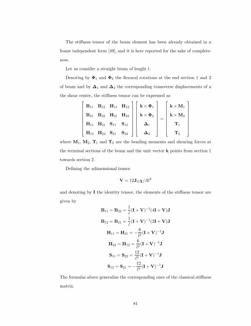
The stiffness tensor of the beam element has been already obtained in a

frame independent form [49], and it is here reported for the sake of complete-

ness.

Let us consider a straight beam of lenght l.

Denoting by Φ1 and Φ2 the flexural rotations at the end section 1 and 2

of beam and by ∆1 and ∆2 the corresponding transverse displacements of a

the shear center, the stiffness tensor can be expressed as

B11 B12 H11 H12

B21 B22 H21 H22

H11 H21 S11 S12

H12 H22 S21 S22

k×Φ1

k×Φ2

∆1

∆2

=

k×M1

k×M2

T1

T2

where M1, M2, T1 and T2 are the bending moments and shearing forces at

the terminal sections of the beam and the unit vector k points from section 1

towards section 2.

Defining the adimensional tensor

V = 12JGχ/Al2

and denoting by I the identity tensor, the elements of the stiffness tensor are

given by

B11 = B22 =1

l(I + V)−1(4I + V)J

B12 = B21 =1

l(I + V)−1(2I + V)J

H11 = H21 = −6

l2(I + V)−1J

H22 = H12 =6

l2(I + V)−1J

S11 = S22 =12

l3(I + V)−1J

S12 = S21 = −12

l3(I + V)−1J

The formulas above generalize the corresponding ones of the classical stiffness

matrix.

81

82

Chapter 5

A BEM approach to the

solution of the torsion and

shear problems

Regardless of the selected approach, either based upon the displacement or the

stress one, the complete solution in terms of displacements and stress fields

for rods of generic cross section can be represented only partially by means

of explicit analytic expressions since some terms associated with torsion and

shear embody auxiliary functions that are solution of Dirichlet or Neumann

problems related to the cross section domain; this is true with the exception

of sections having particular geometries for which a closed-form solution ex-

ists. For all the other cases, the only way to obtain the complete solution of

the problem is to adopt a numerical approach. This chapter illustrates the

operative details leading to expressions which are very simple to implement in

a computer code.

83

5.1 Weak formulation

Weak formulation of the harmonic problem for the determination of ψ (3.46),

combined with the second Green identity leads to the following alternative

characterization of the problem [8] :

−

∫

Ωψχ,ii dA+

∫

∂Ωψχ,ini ds = −

∫

∂ΩχAp (p)n ds . (5.1)

in which χ is an arbitrary weight function sufficiently regular.

By adopting as weight function the so-called fundamental solution of Laplace

equation in the plane

χ∗ = −1

2πln

(

1

||p− p∗||

)

, (5.2)

one obtains the classical integral identity that represent the starting point of

all BEM formulations. In (5.2) p∗ denotes the position vector of an arbitrary

point of the cross section plain and is commonly called source point.

As stated in [8], the function χ∗ is solution of the equation χ∗,ii = δ(p−p∗),

in which δ represent the Dirac distribution; the gradient of (5.2) is given by

gradχ∗ =p− p∗

2π||p− p∗||2. (5.3)

By virtue of the properties of the function χ∗, formula (5.1) becomes:

c(p∗)ψ(p∗)−

∫

∂Ωψ(p)

(p− p∗) · n

2π||p− p∗||2ds =

= −

∫

∂Ω

1

2πln

(

1

||p− p∗||

)

Ap (p)n ds ,

(5.4)

where the coefficient c depends on the position of the point p∗ with respect

to the domain Ω. In particular c(p∗) = 1 if p∗ ∈ Ω, c(p∗) = 0 if p∗ /∈ Ω

and c(p∗) =θ− − θ+

2πif p∗ ∈ ∂Ω, in which θ− and θ+, assumed positive

if counterclockwise, are the angles between the unit vector tangent to the

boundary in a circulation sense respectively clockwise and counterclockwise

on the boundary.

84

Let us now assume that the boundary ∂Ω is polygonal, i.e. it is constituted

by the union of nv sides: ∂Ω =⋃nv

l=1 ∂Ωl. In this particular case, the ge-

ometry of the section results completely defined by the vertexes’ coordinates

p1, ...,pnv. Thus, by introducing the following parametric representation

for the side l:

p(µl) =pl + pl+1

2+ µl

pl+1 − pl

2, l ∈ 1, ..., nv, µl ∈ [−1, 1], (5.5)

the relevant arc length s isds

dµ=

√

dp

dµ·dp

dµ=ll2, so that formula (5.4) assumes

the following expression:

c(p∗)ψ(p∗)−

nv∑

l=1

ll2

∫ 1

−1ψ(µl)

(p(µl)− p∗) · nl

2π||p(µl)− p∗||2dµl =

= −

nv∑

l=1

ll2

∫ 1

−1

1

2πln

(

1

||p(µl)− p∗||

)

Ap (µl)nl dµl ;

(5.6)

in particular, if p∗ belongs to one boundary’s sides, excluding their extremes

points, it turns out to be c(p∗) =1

2.

One can specialize the (5.6) for the first component by obtaining

c(p∗)ψ1(p∗)−

nv∑

l=1

ll2

∫ 1

−1ψ1(µl)

(p(µl)− p∗) · nl

2π||p(µl)− p∗||2dµl =

= −

nv∑

l=1

ll2

∫ 1

−1

1

2πln

(

1

||p(µl)− p∗||

)

[

α(x2n1 + xyn1) + β(x2n1 + y2n2)]

dµl .

(5.7)

5.2 Interpolation

Integral equation (5.6) is converted in algebraic form by using for the restric-

tion of ψ to the generic side l the same interpolation adopted in [61]:

ψ(µl) =

nPl∑

β=1

p(β)l T (β−1)(µl) (5.8)

85

i.e., in scalar form,

ψ1(µl) =nPl∑

β=1

p(β)1l T

(β−1)(µl)

ψ2(µl) =nPl∑

β=1

p(β)2l T

(β−1)(µl)

where l is the index that varies on each side of the polygonal shape, T (β) is

the Chebyshev’s polynomial of degree β and nPl corresponds to the number of

parameters used to interpolate the unknown function ψ. The first six terms

of the polynomial are reported hereafter for the reader’s convenience:

T (0)(µ) = 1 T (1)(µ) = µ T (2)(µ) = 2µ2 − 1

T (3)(µ) = 4µ3 − 3µ T (4)(µ) = 8µ4 − 8µ2 + 1 T (5)(µ) = 16µ5 − 20µ3 + 5µ ;

in general, the polynomial of order β > 1 are obtained by the following recur-

sive expression:

T (β+1)(µ) = 2µT (β)(µ)− T (β−1)(µ), (5.9)

For each side m∗, it is necessary to collocate nPm∗ source points whose

position (p∗)(α∗)m∗ is determined by (5.5) following the ordered sequence of reals

−1 < µ1 < µ2 < ... < µα∗ < ... < nPm∗ < 1.

The total number of source points, that also corresponds to the number of

equations to write, is expressed by N ∗eq, while the total number of unknowns

parameters is denoted by Npar.

5.3 Algebraic solution system

In this section we illustrate the operative details that allow one to re-formulate

(5.6), by using the adopted interpolation functions, in a system of equation

AP∗Q

pQ

= bP∗

, in which P ∗ ∈ 1, ..., N∗eq, Q ∈ 1, ..., Npar and p

Qis the

vector containing the collection of unknown parameters pβl relative to all sides

of the boundary Ω; elements of AP∗Q

and bP∗

will be defined afterwards.

86

The global indices of equations and parameters are set in relation with local

indices by the following relations: P ∗ ← (m∗, α∗), Q← (l, β) ; thus, the first

nP1∗equations of the solution system are those associated with the side 1, the

following nP2∗with side 2 and so on. Analogously, the columns of the A

P∗Q

matrix can be merged in groups whose cardinality is defined by the number

of parameters p(β)l used for each side.

To obtain a number of equations equal to the number of unknowns it is

sufficient to consider on each side a number of source points equal to the

number of the parameters, so that the equivalence N ∗eq = Npar is satisfied.

However, fulfilling this constraint, is possible to use different choices related

to particular modeling requirements.

It is convenient to compute the elements of the matrix AP∗Q

and of the

vector bP∗

by iterating on the local indices m∗, α∗, l and β and, subsequently,

by using correspondences between local and global indices, to lead back these

terms to the global numeration. To obtain expressions that can be directly

implemented it is necessary to specify the dependency of the terms in (5.6)

from the local indices:

1

2ψα∗

m∗ −

nv∑

l=1

ll2

∫ 1

−1ψ(µl)(χ

∗

,n)(α∗)m∗ (µl) dµl =

= −nv∑

l=1

ll2

∫ 1

−1

(χ∗)(α∗)m∗ (µl) A (p)n dµl

(5.10)

For brevity, in the sequel, reference will be made to the first row of the vector

equation (5.10):

1

2ψα∗1

m∗ −

nv∑

l=1

ll2

∫ 1

−1ψ1(µl)(χ

∗

,n)(α∗)m∗ (µl) dµl =

= −

nv∑

l=1

ll2

∫ 1

−1(χ∗)

(α∗)m∗ (µl)

[

α(x2n1 + xyn1) + β(x2n1 + y2n2)]

dµl ,

(5.11)

The term ψα∗1m∗ is obtained from (5.8) by setting µl = µα∗ ; thus, only the

87

parameters of ψ relative to the side m∗ contribute to the term ψα∗1m∗ .

In order to simplify the implementation it is useful to explicit the first term

in (5.10) by introducing the l index:

1

2ψα∗1

m∗ =1

2

nv∑

l=1

nPl∑

β=1

δlm∗p(β)l T (β−1)(µα∗) =

nv∑

l=1

nPl∑

β=1

A(1)m∗α∗lβp

(β)l , (5.12)

in which it is set A(1)m∗α∗lβ = δlm∗

1

2T (β−1)(µα∗). By making explicit the first

integral in (5.10), one obtains:

−

nv∑

l=1

ll2

∫ 1

−1

nPl∑

β=1

p(β)l T (β−1)(µl)

(p(µl)− p∗) · nl

2π||p(µl)− p∗||2dµl =

=

nv∑

l=1

nPl∑

β=1

A(2)m∗α∗lβ p

(β)l

(5.13)

in which:

A(2)m∗α∗lβ = −

ll2

∫ 1

−1T (β−1)(µl)

(p(µl)− p∗) · nl

2π||p(µl)− p∗||2dµl (5.14)

One observes that vector p(µl) − p∗ turns out to be parallel to side l when

l = m∗ so that, although the gradient of χ∗ is singular at the source point, the

scalar product at the numerator in (5.14) is equal to zero.

Finally, for the term that appears at the right-hand side of in (5.10), it

turns out to be:

b1m∗α∗ = −

nv∑

l=1

ll2

∫ 1

−1

1

2πln

(

1

||p(µl)− p∗||

)

[

α(x2n1 + xyn1) + β(x2n1 + y2n2)]

dµl ,

(5.15)

where the position of the source point p∗ is defined by m∗ e α∗ as in the

previous formulas.

5.4 Entries of the solution system matrix

We are now going to illustrate the procedure adopted for computing the inte-

grals (5.14) and (5.18) when the integrand function is singular, what occurs

88

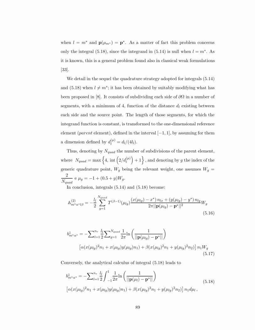
when l = m∗ and p(µm∗) = p∗. As a matter of fact this problem concerns

only the integral (5.18), since the integrand in (5.14) is null when l = m∗. As

it is known, this is a general problem found also in classical weak formulations

[33].

We detail in the sequel the quadrature strategy adopted for integrals (5.14)

and (5.18) when l 6= m∗; it has been obtained by suitably modifying what has

been proposed in [8]. It consists of subdividing each side of ∂Ω in a number of

segments, with a minimum of 4, function of the distance dl existing between

each side and the source point. The length of those segments, for which the

integrand function is constant, is transformed to the one-dimensional reference

element (parent element), defined in the interval [−1, 1], by assuming for them

a dimension defined by d(µ)l = dl/(4ll).

Thus, denoting by Nquad the number of subdivisions of the parent element,

where Nquad = max

4, int(

2/d(µ)l

)

+ 1

, and denoting by g the index of the

generic quadrature point, Wg being the relevant weight, one assumes Wg =

2

Nquade µg = −1 + (0.5 + g)Wg.

In conclusion, integrals (5.14) and (5.18) become:

A(2)m∗α∗lβ = −

ll2

Nquad∑

g=1

T (β−1)(µlg)(x(µlg)− x

∗)nlx + (y(µlg)− y∗)nly

2π||p(µlg)− p∗||2Wg

(5.16)

b1m∗α∗ = −∑nv

l=1

ll2

∑Nquad

g=1

1

2πln

(

1

||p(µlg)− p∗||

)

[

α(x(µlg)2n1 + x(µlg)y(µlg)n1) + β(x(µlg)

2n1 + y(µlg)2n2)

]

n1Wg

(5.17)

Conversely, the analytical calculus of integral (5.18) leads to

b1m∗α∗ = −∑nv

l=1

ll2

∫ 1

−1

1

2πln

(

1

||p(µl)− p∗||

)

[

α(x(µlg)2n1 + x(µlg)y(µlg)n1) + β(x(µlg)

2n1 + y(µlg)2n2)

]

n1dµl ,

(5.18)

89

To implement the analytical and numerical calculus of integrals (5.18) one

needs to explicit the terms p(µl) e p∗ by adopting the parametric representa-

tion previously introduced:

p(µl) = p(med)l +

ll2µl

(

pl+1 − pl

||pl+1 − pl||

)

= p(med)l +

ll2µletl

p∗(µl) = p∗(med)l +

lm∗

2µα∗

(

pl+1 − pl

||pl+1 − pl||

)

= pmm∗ +lm∗

2µm∗etm∗

(5.19)

where et is the unit vector tangent to the segment. When l = m∗, one gets:

p(µl)− p∗ =lm∗

2(µ− µα∗) etm∗ ⇒ ||p(µl)− p∗|| =

lm∗

2|µ− µα∗ |

To explicit the expression of[

α(x2n1 + xyn1) + β(x2n1 + y2n2)]

it is necessary

to write the first formula of (5.19) in components:

x(µl) = xml +1

2µl (xl+1 − xl)

y(µl) = yml +1

2µl (yl+1 − yl)

(5.20)

By squaring both sides of (5.20), one obtains

x2(µl) = x2ml + xml (xl+1 − xl)µl +

1

4(xl+1 − xl)

2 µ2l

y2(µl) = y2ml + yml (yl+1 − yl) µl +

1

4(yl+1 − yl)

2 µ2l

(5.21)

It is also necessary to write the expression of the product of (5.20)

x(µl)y(µl) = xmlyml +1

2yml (xl+1 − xl)µl +

1

2xml (yl+1 − yl)µl+

+1

4(xl+1 − xl) (yl+1 − yl)µ

2l

(5.22)

and explicit the following expression

AP · n = [α(p⊗ p) + β(p · p)I]n =

= α(p · n)p + β(p · p)n =

α(p · n)x+ β(p · p)n1

α(p · n)y + β(p · p)n2

(5.23)

90

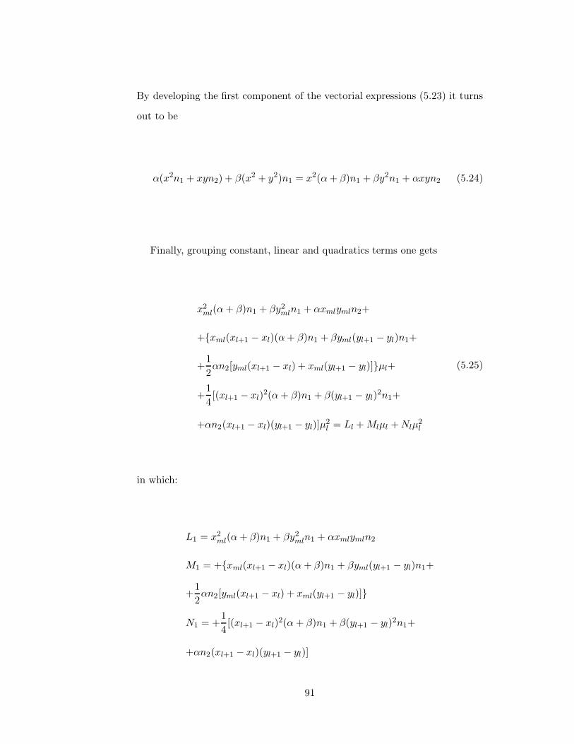
By developing the first component of the vectorial expressions (5.23) it turns

out to be

α(x2n1 + xyn2) + β(x2 + y2)n1 = x2(α+ β)n1 + βy2n1 + αxyn2 (5.24)

Finally, grouping constant, linear and quadratics terms one gets

x2ml(α+ β)n1 + βy2

mln1 + αxmlymln2+

+xml(xl+1 − xl)(α+ β)n1 + βyml(yl+1 − yl)n1+

+1

2αn2[yml(xl+1 − xl) + xml(yl+1 − yl)]µl+

+1

4[(xl+1 − xl)

2(α+ β)n1 + β(yl+1 − yl)2n1+

+αn2(xl+1 − xl)(yl+1 − yl)]µ2l = Ll +Mlµl +Nlµ

2l

(5.25)

in which:

L1 = x2ml(α+ β)n1 + βy2

mln1 + αxmlymln2

M1 = +xml(xl+1 − xl)(α+ β)n1 + βyml(yl+1 − yl)n1+

+1

2αn2[yml(xl+1 − xl) + xml(yl+1 − yl)]

N1 = +1

4[(xl+1 − xl)

2(α + β)n1 + β(yl+1 − yl)2n1+

+αn2(xl+1 − xl)(yl+1 − yl)]

91

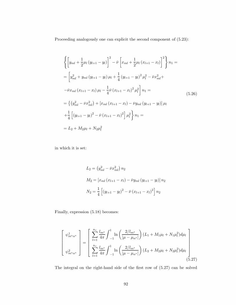
Proceeding analogously one can explicit the second component of (5.23):

[

yml +1

2µl (yl+1 − yl)

]2

− ν

[

xml +1

2µl (xl+1 − xl)

]2

n1 =

=

[

y2ml + yml (yl+1 − yl)µl +

1

4(yl+1 − yl)

2 µ2l − νx

2ml+

−νxml (xl+1 − xl) µl −1

4ν (xl+1 − xl)

2 µ2l

]

n1 =

=(

y2ml − νx

2ml

)

+ [xml (xl+1 − xl)− νyml (yl+1 − yl)]µl

+1

4

[

(yl+1 − yl)2 − ν (xl+1 − xl)

2]

µ2l

n1 =

= L2 +M2µl +N2µ2l

(5.26)

in which it is set:

L2 =(

y2ml − νx

2ml

)

n2

M2 = [xml (xl+1 − xl)− νyml (yl+1 − yl)]n2

N2 =1

4

[

(yl+1 − yl)2 − ν (xl+1 − xl)

2]

n2

Finally, expression (5.18) becomes:

ψ1m∗α∗

ψ2m∗α∗

=

nv∑

l=1

lm∗

4π

∫ 1

−1ln

(

2/lm∗

|µ− µα∗ |

)

(L1 +M1µl +N1µ2l )dµl

nv∑

l=1

lm∗

4π

∫ 1

−1

ln

(

2/lm∗

|µ− µα∗ |

)

(L2 +M2µl +N2µ2l )dµl

(5.27)

The integral on the right-hand side of the first row of (5.27) can be solved

92

analytically as follows

lm∗

4π

1∫

−1

[

−L1 ln

(

lm∗

2

)

−M1 ln

(

lm∗

2

)

µl −N1 ln

(

lm∗

2

)

µ2l +

+L1 ln

(

1

|µl − µα∗ |

)

+M1 ln

(

1

|µl − µα∗ |

)

µl+

+N1 ln

(

1

|µl − µα∗ |

)

µ2l

]

dµl =lm∗

4π

[

− ln

(

lm∗

2

)

(2L1 +2

3N1)+

+L1H(1)α∗ +M1H

(2)α∗ +N1H

(3)α∗

]

where

H(1)α∗ =

∫ 1

−1

ln1

|µl − µα∗ |dµl

H(2)α∗ =

∫ 1

−1µlln

1

|µ− µα∗ |dµl

H(3)α∗ =

∫ 1

−1µ2

l ln1

|µ− µα∗ |dµl

(5.28)

These integrals can be calculated analytically:

H(1)α∗ = 2− ln

(

1− µ2α∗

)

+ µα∗ ln

(

1− µα∗

1 + µα∗

)

H(2)α∗ = µα∗ +

1

2ln

(

1 + µα∗

1− µα∗

)

+1

2µ2

α∗ ln

(

1− µα∗

1 + µα∗

)

H(3)α∗ =

1

3[ln(1− µα∗)− ln(1 + µα∗)]µ3

α∗ +2

3µ2

α∗ +2

9+

−1

3ln(1− µα∗)−

1

3ln(1 + µα∗)

(5.29)

by obtaining expressions that are well-defined for −1 < µα∗ < 1.

93

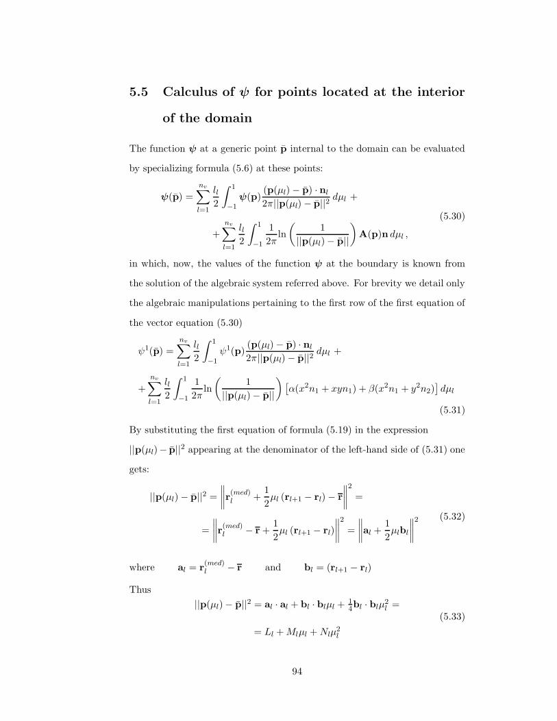
5.5 Calculus of ψ for points located at the interior

of the domain

The function ψ at a generic point p internal to the domain can be evaluated

by specializing formula (5.6) at these points:

ψ(p) =

nv∑

l=1

ll2

∫ 1

−1ψ(p)

(p(µl)− p) · nl

2π||p(µl)− p||2dµl +

+nv∑

l=1

ll2

∫ 1

−1

1

2πln

(

1

||p(µl)− p||

)

A(p)n dµl ,

(5.30)

in which, now, the values of the function ψ at the boundary is known from

the solution of the algebraic system referred above. For brevity we detail only

the algebraic manipulations pertaining to the first row of the first equation of

the vector equation (5.30)

ψ1(p) =nv∑

l=1

ll2

∫ 1

−1

ψ1(p)(p(µl)− p) · nl

2π||p(µl)− p||2dµl +

+

nv∑

l=1

ll2

∫ 1

−1

1

2πln

(

1

||p(µl)− p||

)

[

α(x2n1 + xyn1) + β(x2n1 + y2n2)]

dµl

(5.31)

By substituting the first equation of formula (5.19) in the expression

||p(µl)− p||2 appearing at the denominator of the left-hand side of (5.31) one

gets:

||p(µl)− p||2 =

∥

∥

∥

∥

r(med)l +

1

2µl (rl+1 − rl)− r

∥

∥

∥

∥

2

=

=

∥

∥

∥

∥

r(med)l − r +

1

2µl (rl+1 − rl)

∥

∥

∥

∥

2

=

∥

∥

∥

∥

al +1

2µlbl

∥

∥

∥

∥

2 (5.32)

where al = r(med)l − r and bl = (rl+1 − rl)

Thus

||p(µl)− p||2 = al · al + bl · blµl + 14bl · blµ

2l =

= Ll +Mlµl +Nlµ2l

(5.33)

94

in which

Al = al · al =∥

∥

∥r(med)l − r

∥

∥

∥

2

Bl = al · bl = (rl+1 − rl)(

r(med)l − r

)

Cl =1

4bl · bl = ‖rl+1 − rl‖

2

One can now substitute the first equation of (5.19) in the expression

(p(µl)− p) · nl that appears at the numerator of the first integrand of (5.31):

[

r(med)l + 1

2µl (rl+1 − rl)− r]

· nl =

=(

r(med)l − r

)

· nl + 12µl (rl+1 − rl) · nl

(5.34)

Since (rl+1 − rl) is orthogonal to nl , the second term on the right-hand side

of the expression above vanishes and the final result is

(p(µl)− p) · nl =(

r(med)l − r

)

· nl = Dl (5.35)

Further, by exploiting properties of the logarithm, it is possible to re-write the

expression appearing in the second sum of (5.31) to obtain:

∫ 1

−1ln (‖r (µl)− r‖)−1(Ll +Mlµl +Nlµ

2l

)

dµl =

= −1

2

∫ 1

−1

ln(

‖r (µl)− r‖2)

(

Ll +Mlµl +Nlµ2l

)

dµl

Thus, formula (5.31) can be implemented by means of the following expres-

sions:

ψ1(p) =

nv∑

l=1

ll4π

nPl∑

β=1

Ψ(β)l p

(β)l1 −

nv∑

l=1

ll8π

(

Q(1)l + Q

(2)l + Q

(3)l

)

, (5.36)

95

where

Ψ(β)l =

∫ 1

−1

T (β−1)(µl)Dl

[

Al + Blµl + Clµ2l

] dµl ,

Q(1)l = L1

∫ 1

−1ln[

Al + Blµl + Clµ2l

]

dµ ,

Q(2)l = M1

∫ 1

−1µlln

[

Al + Blµl + Clµ2l

]

dµl ,

Q(3)l = N1

∫ 1

−1µ2

l ln[

Al + Blµl + Clµ2l

]

dµl

(5.37)

Integrals (5.37), also amenable to analytical computation are evaluated nu-

merically as in (5.16) and (5.17).

96

5.6 Calculus of derivatives of ψ for points located

at the interior of the domain

To obtain the values of τ for points internal to Ω one needs to calculate the

gradient of ψ at these points. By deriving (5.36) with respect to p one obtains:

∂ψ1

∂p(p) =

nv∑

l=1

ll4π

nPl∑

β=1

∂Ψ(β)l

∂pp(β)l1 +

−

nv∑

l=1

ll8π

(

∂Q(1)l

∂p+∂Q

(2)l

∂p+∂Q

(3)l

∂p

)

(5.38)

Having set ρ(µl, p) = Al + Blµl + Clµ2l , derivatives in (5.38) become:

∂Ψl

∂p

(β)

=

∫ 1

−1T (β−1)(µl)

1

ρ2

(

−ρn−∂ρ

∂pDl

)

dµl (5.39)

∂Ql

∂p

(1)

=

∫ 1

−1

L1

ρ

∂ρ

∂pdµl

∂Ql

∂p

(2)

=

∫ 1

−1

M1µl

ρ

∂ρ

∂pdµl

∂Ql

∂p

(3)

=

∫ 1

−1

N1µ2l

ρ

∂ρ

∂pdµl

(5.40)

∂ρ

∂p= −2

(

p(med)l − p

)

− (pl+1 − pl) µl . (5.41)

97

98

Chapter 6

Numerical results

To investigate the computational efficiency as well as the accuracy of the

proposed numerical solution, the expressions of stress field, of shear center

and of shear deformability tensor reported in the previous chapters have been

implemented in a Matlab code. In this respect we recall that the particular

BEM method implemented here allows one to obtain the results by assigning

only the vertices of the section, similarly to flexure.

The results of the BEM solution for circular and rectangular domain have

been first compared with the available closed-form solutions. However, these

last ones don’t take into account the Poisson’s ratio dependency. Hence, a

series of numerical tests on some sections have been performed in order to

make a comparison with results from literature.

99

6.1 Rectangular cross section

Let us consider a rectangular section assigned by means of the following ver-

tices:

l : 1 2 3 4

x : -0.5 0.5 0.5 -0.5

y : -1 -1 1 1

−0.6 −0.4 −0.2 0 0.2 0.4 0.6

−1

−0.8

−0.6

−0.4

−0.2

0

0.2

0.4

0.6

0.8

1

The resulting shear factor χNUM11 is compared with the corresponding an-

alytical value χan.11 [23] obtained in the case ν = 0. Specifically tab.1 reports

the error e = |χNUM11 − χan.

11 |/χan.11 as function of the number of polynomials

assumed to interpolate each side of the polygonal.

100

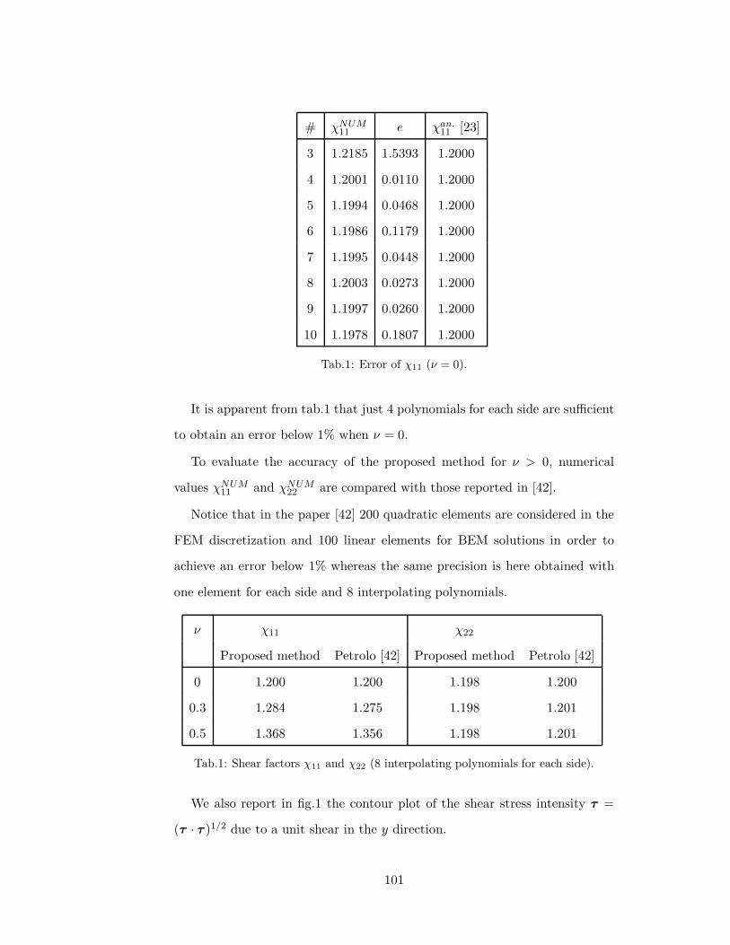
# χNUM11 e χan.

11 [23]

3 1.2185 1.5393 1.2000

4 1.2001 0.0110 1.2000

5 1.1994 0.0468 1.2000

6 1.1986 0.1179 1.2000

7 1.1995 0.0448 1.2000

8 1.2003 0.0273 1.2000

9 1.1997 0.0260 1.2000

10 1.1978 0.1807 1.2000

Tab.1: Error of χ11 (ν = 0).

It is apparent from tab.1 that just 4 polynomials for each side are sufficient

to obtain an error below 1% when ν = 0.

To evaluate the accuracy of the proposed method for ν > 0, numerical

values χNUM11 and χNUM

22 are compared with those reported in [42].

Notice that in the paper [42] 200 quadratic elements are considered in the

FEM discretization and 100 linear elements for BEM solutions in order to

achieve an error below 1% whereas the same precision is here obtained with

one element for each side and 8 interpolating polynomials.

ν χ11 χ22

Proposed method Petrolo [42] Proposed method Petrolo [42]

0 1.200 1.200 1.198 1.200

0.3 1.284 1.275 1.198 1.201

0.5 1.368 1.356 1.198 1.201

Tab.1: Shear factors χ11 and χ22 (8 interpolating polynomials for each side).

We also report in fig.1 the contour plot of the shear stress intensity τ =

(τ · τ )1/2 due to a unit shear in the y direction.

101

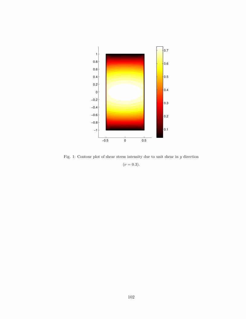
−0.5 0 0.5

−1

−0.8

−0.6

−0.4

−0.2

0

0.2

0.4

0.6

0.8

1

0.1

0.2

0.3

0.4

0.5

0.6

0.7

Fig. 1: Contour plot of shear stress intensity due to unit shear in y direction

(ν = 0.3).

102

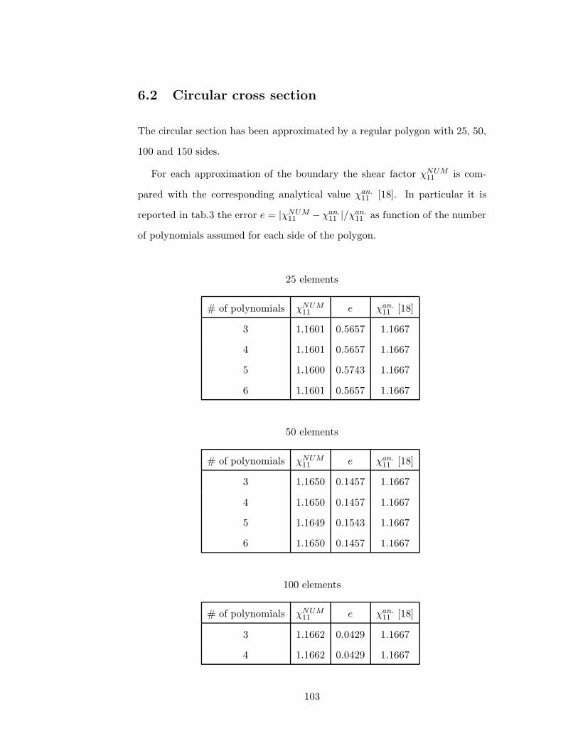
6.2 Circular cross section

The circular section has been approximated by a regular polygon with 25, 50,

100 and 150 sides.

For each approximation of the boundary the shear factor χNUM11 is com-

pared with the corresponding analytical value χan.11 [18]. In particular it is

reported in tab.3 the error e = |χNUM11 − χan.

11 |/χan.11 as function of the number

of polynomials assumed for each side of the polygon.

25 elements

# of polynomials χNUM11 e χan.

11 [18]

3 1.1601 0.5657 1.1667

4 1.1601 0.5657 1.1667

5 1.1600 0.5743 1.1667

6 1.1601 0.5657 1.1667

50 elements

# of polynomials χNUM11 e χan.

11 [18]

3 1.1650 0.1457 1.1667

4 1.1650 0.1457 1.1667

5 1.1649 0.1543 1.1667

6 1.1650 0.1457 1.1667

100 elements

# of polynomials χNUM11 e χan.

11 [18]

3 1.1662 0.0429 1.1667

4 1.1662 0.0429 1.1667

103

150 elements

# of polynomials χNUM11 e χan.

11 [18]

3 1.1665 0.0171 1.1667

Tab.3: comparison between χNUM

11and the corresponding analytical value χan.

11[18].

The tables above show that a finer discretization of the boundary produces

an error decrease higher then that achieved by increasing the number of poly-

nomials for each side of the polygon.

104

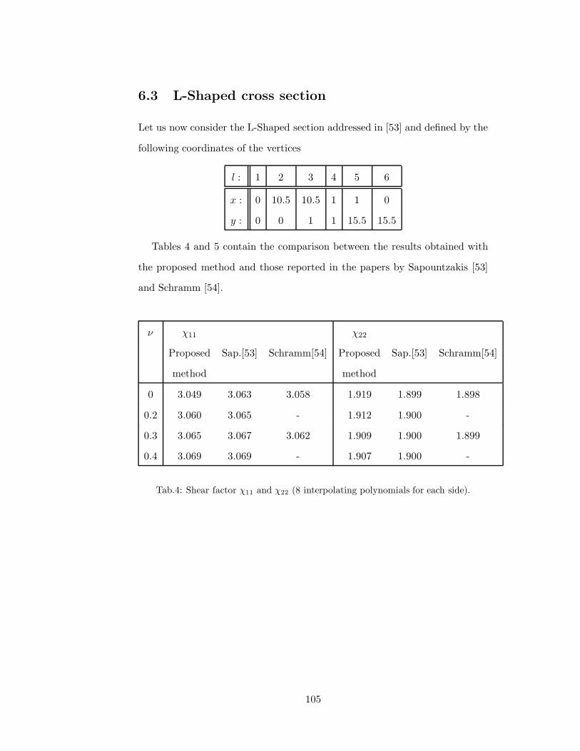
6.3 L-Shaped cross section

Let us now consider the L-Shaped section addressed in [53] and defined by the

following coordinates of the vertices

l : 1 2 3 4 5 6

x : 0 10.5 10.5 1 1 0

y : 0 0 1 1 15.5 15.5

Tables 4 and 5 contain the comparison between the results obtained with

the proposed method and those reported in the papers by Sapountzakis [53]

and Schramm [54].

ν χ11 χ22

Proposed Sap.[53] Schramm[54] Proposed Sap.[53] Schramm[54]

method method

0 3.049 3.063 3.058 1.919 1.899 1.898

0.2 3.060 3.065 - 1.912 1.900 -

0.3 3.065 3.067 3.062 1.909 1.900 1.899

0.4 3.069 3.069 - 1.907 1.900 -

Tab.4: Shear factor χ11 and χ22 (8 interpolating polynomials for each side).

105

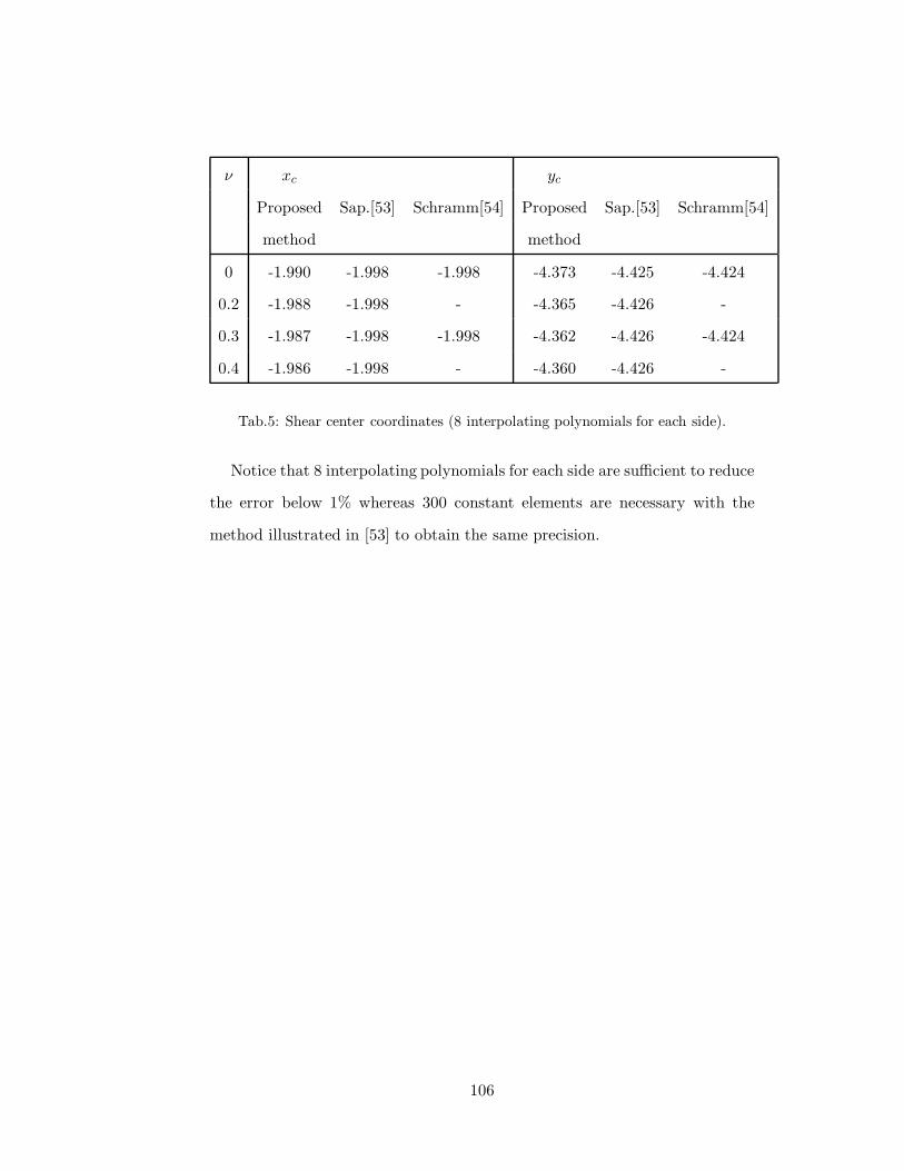
ν xc yc

Proposed Sap.[53] Schramm[54] Proposed Sap.[53] Schramm[54]

method method

0 -1.990 -1.998 -1.998 -4.373 -4.425 -4.424

0.2 -1.988 -1.998 - -4.365 -4.426 -

0.3 -1.987 -1.998 -1.998 -4.362 -4.426 -4.424

0.4 -1.986 -1.998 - -4.360 -4.426 -

Tab.5: Shear center coordinates (8 interpolating polynomials for each side).

Notice that 8 interpolating polynomials for each side are sufficient to reduce

the error below 1% whereas 300 constant elements are necessary with the

method illustrated in [53] to obtain the same precision.

106

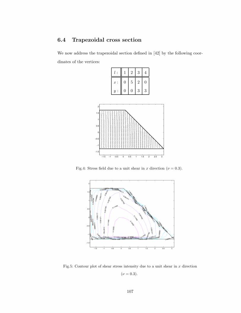
6.4 Trapezoidal cross section

We now address the trapezoidal section defined in [42] by the following coor-

dinates of the vertices:

l : 1 2 3 4

x : 0 5 2 0

y : 0 0 3 3

−1.5 −1 −0.5 0 0.5 1 1.5 2 2.5 3

−1.5

−1

−0.5

0

0.5

1

1.5

2

Fig.4: Stress field due to a unit shear in x direction (ν = 0.3).

1.4665e−008

1.4

665e−008

1.4

665e−008

1.4

665e−008

1.4665e−008

1.4665e−0081.4665e−008

1.4

665e−008

1.4

665e−

008

1.4

665e−

008

0.016294

0.0

16294

0.0

16294

0.0

16294

0.0162940.016294

0.016294

0.0

16294

0.0

16294

0.032588

0.0

32588

0.0

32588

0.0

32588

0.0325880.032588

0.032588

0.0

32588

0.0

32588

0.0

48882

0.048882

0.0

48882

0.048882

0.0

48882

0.0488820.048882

0.0

48882

0.0

65177

0.065177

0.065177

0.0

65177

0.065177

0.065177

0.0

65177

0.0

65177

0.0

81471

0.081471

0.0

81471

0.0

81471

0.0814710.081471

0.0

81471

0.0

97765

0.0

97765

0.0

97765

0.0

97765

0.097765

0.0

97765

0.0

97765

0.11406

0.1

1406

0.11406

0.11406

0.1

1406

0.1

3035

0.13035

0.1

3035

−1.5 −1 −0.5 0 0.5 1 1.5 2 2.5 3

−1.5

−1

−0.5

0

0.5

1

1.5

2

Fig.5: Contour plot of shear stress intensity due to a unit shear in x direction

(ν = 0.3).

107

−1.5 −1 −0.5 0 0.5 1 1.5 2 2.5 3

−1.5

−1

−0.5

0

0.5

1

1.5

2

Fig.6: Stress field due to unit shear in y direction (ν = 0.3).

2.2926e−008 2.2

926e−008

2.2

926e−008

2.2

926e−008

2.2926e−0082.2926e−0082.2926e−008

2.2

926e−

008

2.2

926e−

008

0.032751

0.0

32751

0.0

32751

0.0

32751

0.0327510.0327510.032751

0.0

32751

0.065502

0.0

65502

0.0

65502

0.065502

0.065502

0.0

65502

0.0

65502

0.098253

0.0

98253

0.0

98253

0.0982530.098253

0.0

98253 0.131

0.1

31

0.1

31

0.131

0.131

0.16376

0.1

6376

0.1

6376

−1.5 −1 −0.5 0 0.5 1 1.5 2 2.5 3

−1.5

−1

−0.5

0

0.5

1

1.5

2

Fig.7: Contour plot of shear stress intensity due to a unit shear in y direction

(ν = 0.3).

Proposed Petrolo[42]

method

xc 1.637 1.637

yc 1.412 1.389

Tab.6: Shear center coordinates.

108

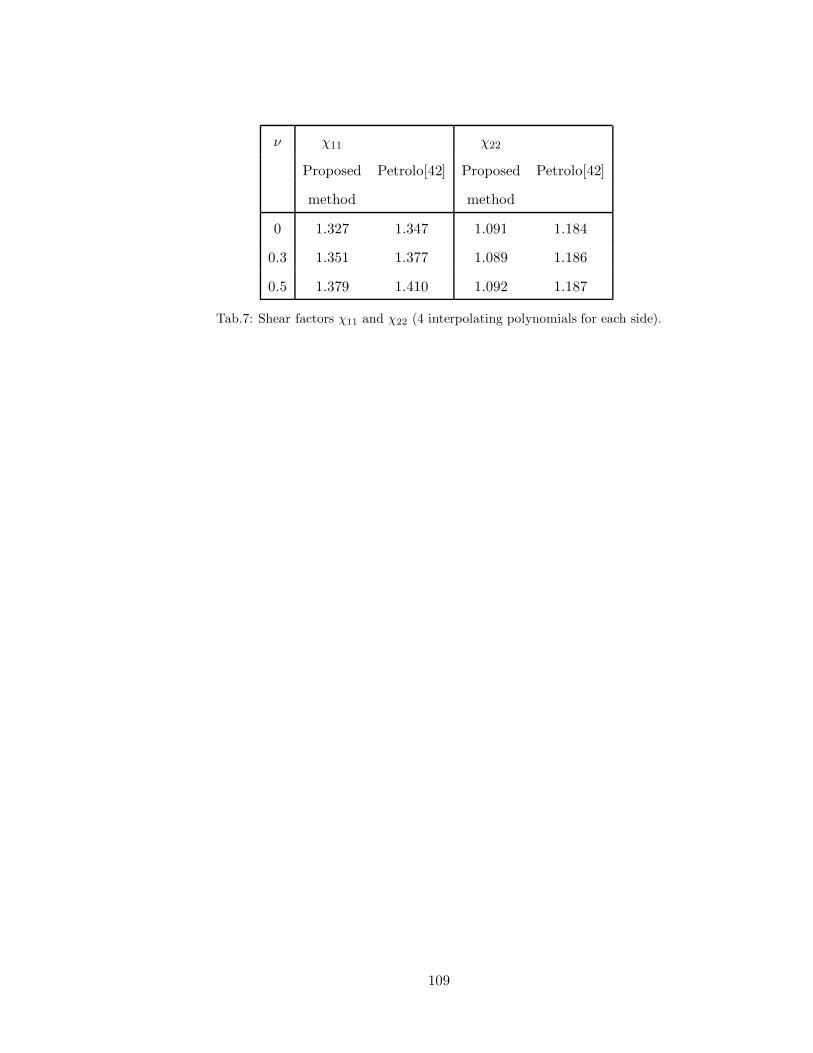
ν χ11 χ22

Proposed Petrolo[42] Proposed Petrolo[42]

method method

0 1.327 1.347 1.091 1.184

0.3 1.351 1.377 1.089 1.186

0.5 1.379 1.410 1.092 1.187

Tab.7: Shear factors χ11 and χ22 (4 interpolating polynomials for each side).

109

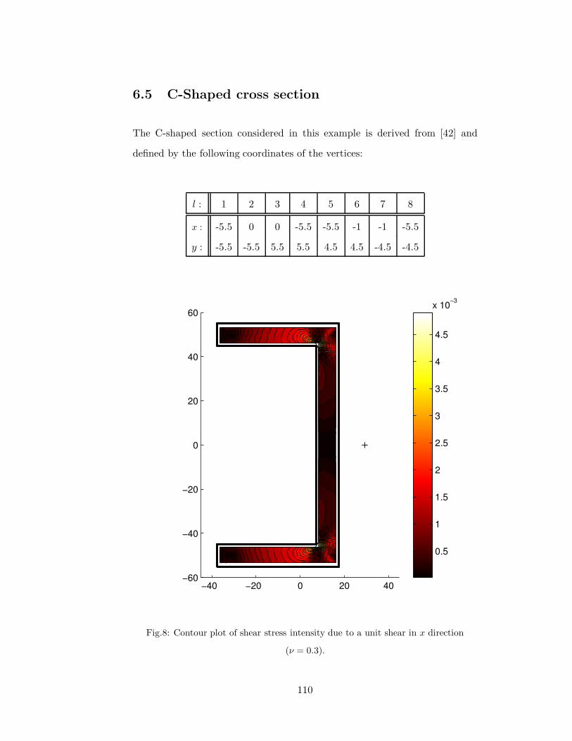
6.5 C-Shaped cross section

The C-shaped section considered in this example is derived from [42] and

defined by the following coordinates of the vertices:

l : 1 2 3 4 5 6 7 8

x : -5.5 0 0 -5.5 -5.5 -1 -1 -5.5

y : -5.5 -5.5 5.5 5.5 4.5 4.5 -4.5 -4.5

−40 −20 0 20 40−60

−40

−20

0

20

40

60

0.5

1

1.5

2

2.5

3

3.5

4

4.5

x 10−3

Fig.8: Contour plot of shear stress intensity due to a unit shear in x direction

(ν = 0.3).

110

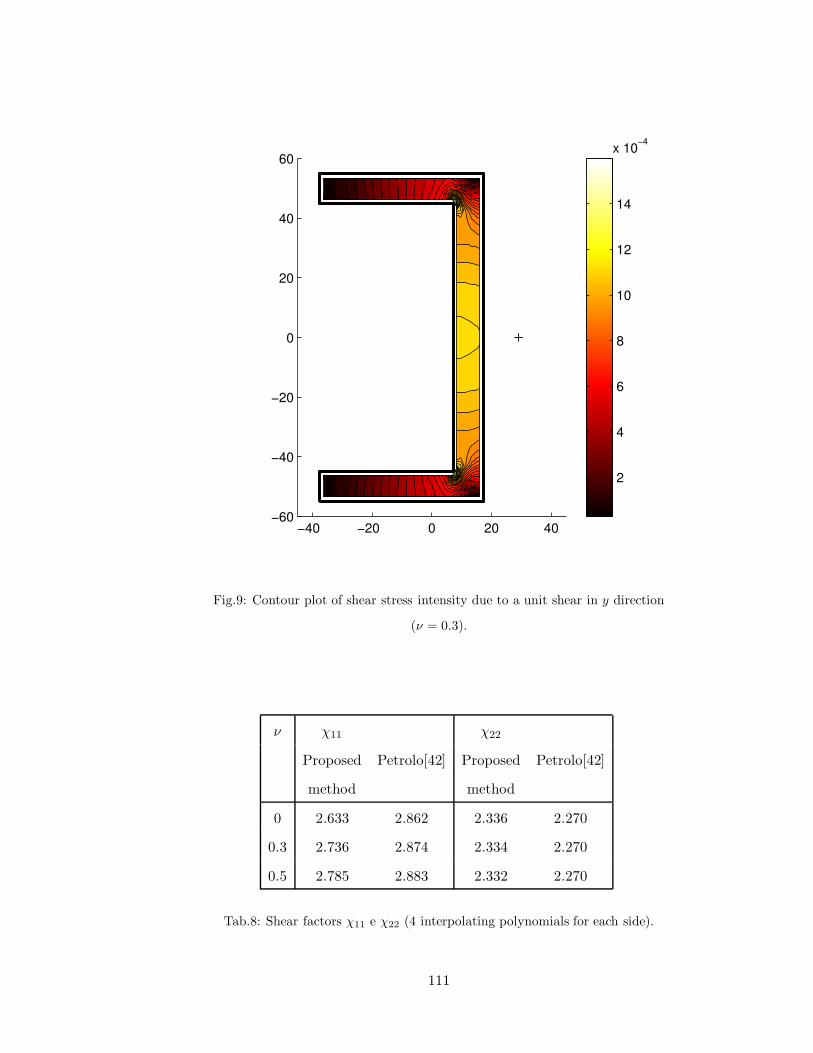
−40 −20 0 20 40−60

−40

−20

0

20

40

60

2

4

6

8

10

12

14

x 10−4

Fig.9: Contour plot of shear stress intensity due to a unit shear in y direction

(ν = 0.3).

ν χ11 χ22

Proposed Petrolo[42] Proposed Petrolo[42]

method method

0 2.633 2.862 2.336 2.270

0.3 2.736 2.874 2.334 2.270

0.5 2.785 2.883 2.332 2.270

Tab.8: Shear factors χ11 e χ22 (4 interpolating polynomials for each side).

111

Proposed Petrolo[42]

method

xc 29.25 30.38

yc 0 0

Tab.9: Shear center coordinates (4 interpolating polynomials for each side).

112

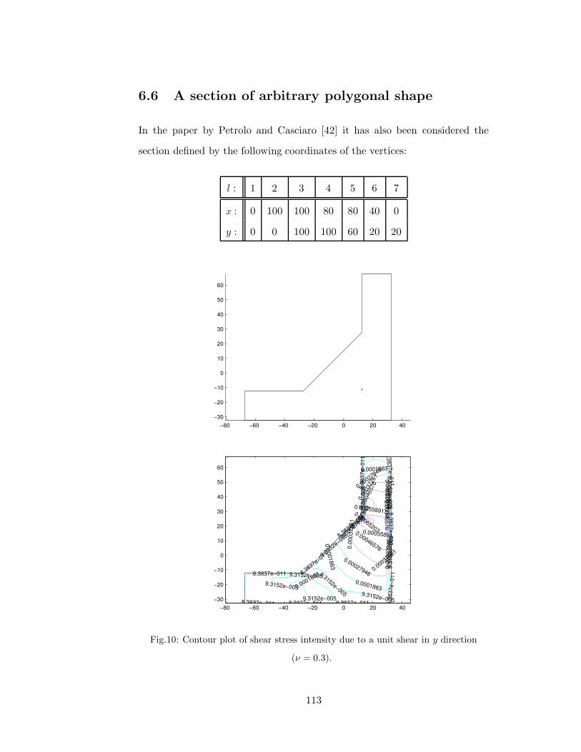
6.6 A section of arbitrary polygonal shape

In the paper by Petrolo and Casciaro [42] it has also been considered the

section defined by the following coordinates of the vertices:

l : 1 2 3 4 5 6 7

x : 0 100 100 80 80 40 0

y : 0 0 100 100 60 20 20

−80 −60 −40 −20 0 20 40

−30

−20

−10

0

10

20

30

40

50

60

8.3837e−011 8.3837e−011

8.3837e−011

8.3

837e−

011

8.3

837e−

011

8.3

837e−

011

8.3

837e−

011

8.3837e−0118.3837e−0118.3837e−011

9.3

152e−

005

9.3

152e−

005

9.3152e−005

9.3152e−005

9.3152e−

005

9.3

152e−

005

9.3152e−005

9.3152e−005

9.3152e−005

0.0

001863

0.0

001863

0.0001863

0.0

001863

0.0

001863

0.0001863

0.0001863

0.0

0027946

0.0

0027946

0.00027946

0.00027946

0.00027946

0.0

0037261

0.00037261

0.0

0037261

0.0

0037261

0.0

0046576

0.00046576

0.0

0046576

0.00055891

0.000558910.00065207

−80 −60 −40 −20 0 20 40

−30

−20

−10

0

10

20

30

40

50

60

Fig.10: Contour plot of shear stress intensity due to a unit shear in y direction

(ν = 0.3).

113

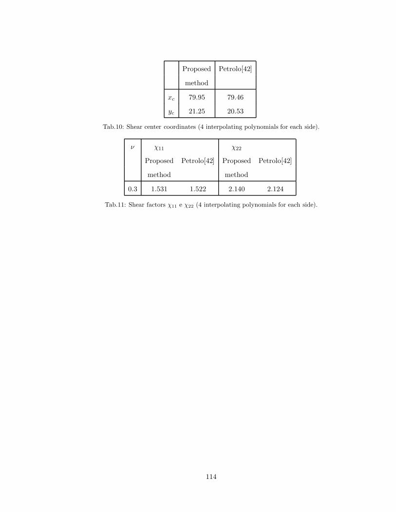
Proposed Petrolo[42]

method

xc 79.95 79.46

yc 21.25 20.53

Tab.10: Shear center coordinates (4 interpolating polynomials for each side).

ν χ11 χ22

Proposed Petrolo[42] Proposed Petrolo[42]

method method

0.3 1.531 1.522 2.140 2.124

Tab.11: Shear factors χ11 e χ22 (4 interpolating polynomials for each side).

114

Chapter 7

Appendix

7.1 Examples of application of the Gibbs rule

Aim of this subsection is to present a systematic derivation of several differ-

ential identities in order to provide examples of application of the Gibbs rule.

The objective is not to prove new identities but to illustrate a methodology

which, on one side, simplifies the derivation of differential identities by means

of the definition of vector product between vectors and tensors introduced in

(2.6) and, on the other, allows one to express the final result in a manner

consistent with the proposed formalism.

For greater clarity each formula is reported in intrinsic notation followed by

the relevant proof in Gibbs notation. We shall make reference to scalar fields

ϕ and ψ, vector fields a and b and a tensor field A; each field is assumed to

be smooth enough to make well defined the relevant differential operation in

which it is involved.

• grad(ϕψ) = (grad ϕ)ψ+ ϕ grad ψ

∇(ϕψ) = (∇ϕ)ψ + ϕ(∇ψ) (7.1)

see, e.g., the definition (2.32)1.

115

• grad(ϕa) = a⊗ grad ϕ+ ϕgrad a

(ϕa)⊗∇ = a⊗ (ϕ∇) + ϕ(a⊗∇)

see, e.g., the definitions (2.32)1 and (2.32)2

• grad(a · b) = (grad a)tb + (grad b)ta

∇(a · b) = ∇(a · b) + ∇(b · a) = (∇⊗ a)b + (∇⊗ b)a (7.2)

see, e.g., the definitions (2.32)1 and (2.32)2

• grad(a×b) = (grad a)×b+a× (grad b) = a× (grad b)−b× (grad a)

(a× b)⊗∇ = (a⊗∇)× b + a× (b⊗∇)

see, e.g., the definitions (2.19)1 and (2.32)2

Remark 1 Notice that the extended Gibbs rule has been applied to the first

addend on the right-hand side in implicit form in the sense that bringing the

factor a into direct connection with⊗∇ would lead to an expression ×b(a⊗∇)

deprived of any significance

• grad(ϕA) = A⊗ (grad ϕ) + ϕ grad A

(ϕA)⊗∇ = A⊗ (ϕ∇) + ϕ(A⊗∇)

see, e.g., the definitions (2.32)1, (2.32)2 and (2.37)

• div (ϕa) = (grad ϕ) · a + ϕ div a

(ϕa) ·∇ = a · (ϕ∇) + ϕ(a ·∇)

see, e.g., the definitions (2.32)1 and (2.32)3

116

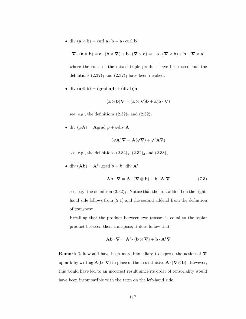
• div (a× b) = curl a · b− a · curl b

∇ · (a× b) = a · (b×∇) + b · (∇× a) = −a · (∇× b) + b · (∇× a)

where the rules of the mixed triple product have been used and the

definitions (2.32)3 and (2.32)4 have been invoked.

• div (a⊗ b) = (grad a)b + (div b)a

(a⊗ b)∇ = (a⊗∇)b + a(b ·∇)

see, e.g., the definitions (2.32)2 and (2.32)3

• div (ϕA) = Agrad ϕ+ ϕdiv A

(ϕA)∇ = A(ϕ∇) + ϕ(A∇)

see, e.g., the definitions (2.32)1, (2.32)3 and (2.33)1

• div (Ab) = At · grad b + b · div At

Ab ·∇ = A · (∇⊗ b) + b ·At∇ (7.3)

see, e.g., the definition (2.32)3. Notice that the first addend on the right-

hand side follows from (2.1) and the second addend from the definition

of transpose.

Recalling that the product between two tensors is equal to the scalar

product between their transpose, it does follow that:

Ab ·∇ = At · (b⊗∇) + b ·At∇

Remark 2 It would have been more immediate to express the action of ∇

upon b by writing A(b ·∇) in place of the less intuitive A · (∇⊗b). However,

this would have led to an incorrect result since its order of tensoriality would

have been incompatible with the term on the left-hand side.

117

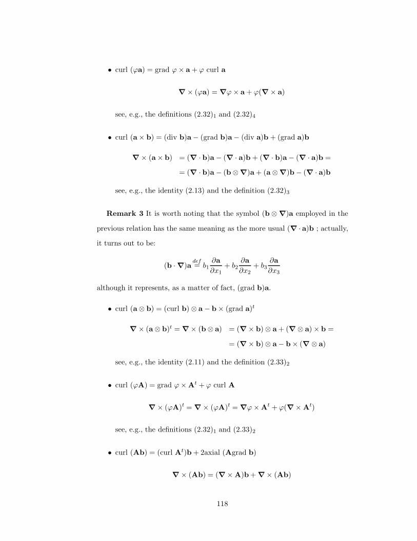
• curl (ϕa) = grad ϕ× a + ϕ curl a

∇× (ϕa) = ∇ϕ× a + ϕ(∇× a)

see, e.g., the definitions (2.32)1 and (2.32)4

• curl (a× b) = (div b)a− (grad b)a− (div a)b + (grad a)b

∇× (a× b) = (∇ · b)a− (∇ · a)b + (∇ · b)a− (∇ · a)b =

= (∇ · b)a− (b⊗∇)a + (a⊗∇)b− (∇ · a)b

see, e.g., the identity (2.13) and the definition (2.32)3

Remark 3 It is worth noting that the symbol (b⊗∇)a employed in the

previous relation has the same meaning as the more usual (∇ · a)b ; actually,

it turns out to be:

(b ·∇)adef= b1

∂a

∂x1+ b2

∂a

∂x2+ b3

∂a

∂x3

although it represents, as a matter of fact, (grad b)a.

• curl (a⊗ b) = (curl b)⊗ a− b× (grad a)t

∇× (a⊗ b)t = ∇× (b⊗ a) = (∇× b)⊗ a + (∇⊗ a)× b =

= (∇× b)⊗ a− b× (∇⊗ a)

see, e.g., the identity (2.11) and the definition (2.33)2

• curl (ϕA) = grad ϕ×At + ϕ curl A

∇× (ϕA)t = ∇× (ϕA)t = ∇ϕ×At + ϕ(∇×At)

see, e.g., the definitions (2.32)1 and (2.33)2

• curl (Ab) = (curl At)b + 2axial (Agrad b)

∇× (Ab) = (∇×A)b + ∇× (Ab)

118

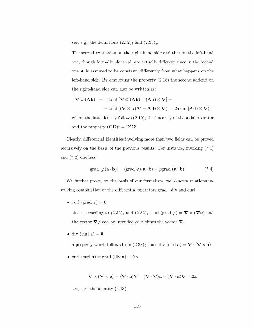
see, e.g., the definitions (2.32)4 and (2.33)2.

The second expression on the right-hand side and that on the left-hand

one, though formally identical, are actually different since in the second

one A is assumed to be constant, differently from what happens on the

left-hand side. By employing the property (2.18) the second addend on

the right-hand side can also be written as:

∇× (Ab) = −axial [∇⊗ (Ab)− (Ab)⊗∇] =

= −axial [(∇⊗ b)At −A(b⊗∇)] = 2axial [A(b⊗∇)]

where the last identity follows (2.10), the linearity of the axial operator

and the property (CD)t = DtCt.

Clearly, differential identities involving more than two fields can be proved

recursively on the basis of the previous results. For instance, invoking (7.1)

and (7.2) one has:

grad [ϕ(a · b)] = (grad ϕ)(a · b) + ϕgrad (a · b) (7.4)

We further prove, on the basis of our formalism, well-known relations in-

volving combination of the differential operators grad , div and curl .

• curl (grad ϕ) = 0

since, according to (2.32)1 and (2.32)4, curl (grad ϕ) = ∇ × (∇ϕ) and

the vector ∇ϕ can be intended as ϕ times the vector ∇.

• div (curl a) = 0

a property which follows from (2.38)2 since div (curl a) = ∇ · (∇× a) .

• curl (curl a) = grad (div a)−∆a

∇× (∇× a) = (∇ · a)∇− (∇ ·∇)a = (∇ · a)∇−∆a

see, e.g., the identity (2.13)

119

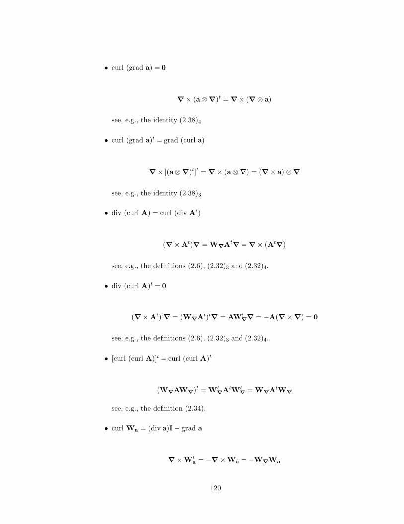
• curl (grad a) = 0

∇× (a⊗∇)t = ∇× (∇⊗ a)

see, e.g., the identity (2.38)4

• curl (grad a)t = grad (curl a)

∇× [(a⊗∇)t]t = ∇× (a⊗∇) = (∇× a) ⊗∇

see, e.g., the identity (2.38)3

• div (curl A) = curl (div At)

(∇×At)∇ = W∇At∇ = ∇× (At

∇)

see, e.g., the definitions (2.6), (2.32)3 and (2.32)4.

• div (curl A)t = 0

(∇×At)t∇ = (W∇At)t

∇ = AWt∇

∇ = −A(∇×∇) = 0

see, e.g., the definitions (2.6), (2.32)3 and (2.32)4.

• [curl (curl A)]t = curl (curl A)t

(W∇AW∇)t = Wt∇

AtWt∇

= W∇AtW∇

see, e.g., the definition (2.34).

• curl Wa = (div a)I− grad a

∇×Wta = −∇×Wa = −W∇Wa

120

see, e.g., the identity (2.15) and the definition (2.33)2.

• curl a = −div Wa

∇×a = −a×∇ = −Wa∇−∇×Wa = −W∇Wa = −(a⊗∇)+(a·∇)I

(7.5)

see, e.g., the definitions (2.32)4 and (2.33)1.

• grad [ϕ div a] = (grad ϕ) div a + ϕ grad (div a) = (grad ϕ)div a +

ϕ div (grad a)t]

∇[ϕ(∇ · a)] = (∇ϕ)(∇ · a) + ϕ(∇ · a)∇

= (∇ϕ)(∇ · a) + ϕ(∇⊗ a)∇

(7.6)

see, e.g., the identity (7.1).

• div [(grad a)a] = (grad a) · (grad a)t + a · div (grada)t = (grad a) ·

(grad a)t + a · grad (div a)

∇ · [(a⊗∇)a] = (∇⊗ a) · (a⊗∇) + a · [(∇⊗ a)∇]

= (a⊗∇) · (∇⊗ a) + a · [(∇ · a)]

(7.7)

see, e.g., the identity (7.3).

Additional differential identities and relations fulfilled by the differential

operators grad , div and curl can be proved in a similar way.

7.2 Matrix representation of the fourth-order ten-

sor Wa Wa

Let us denote by Wa the skew-symmetric rank-two tensor associated with

an arbitrary vector a = a1, a2, a3t. Recalling that the matrix [Wa] has

121

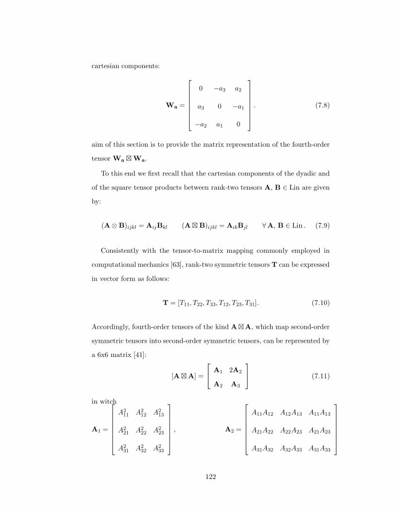
cartesian components:

Wa =

0 −a3 a2

a3 0 −a1

−a2 a1 0

. (7.8)

aim of this section is to provide the matrix representation of the fourth-order

tensor Wa Wa.

To this end we first recall that the cartesian components of the dyadic and

of the square tensor products between rank-two tensors A, B ∈ Lin are given

by:

(A⊗B)ijkl = AijBkl (A B)ijkl = AikBjl ∀A, B ∈ Lin . (7.9)

Consistently with the tensor-to-matrix mapping commonly employed in

computational mechanics [63], rank-two symmetric tensors T can be expressed

in vector form as follows:

T = [T11, T22, T33, T12, T23, T31]. (7.10)

Accordingly, fourth-order tensors of the kind A A, which map second-order

symmetric tensors into second-order symmetric tensors, can be represented by

a 6x6 matrix [41]:

[A A] =

A1 2A2

A2 A3

(7.11)

in witch

A1 =

A211 A2

12 A213

A221 A2

22 A223

A231 A2

32 A233

, A2 =

A11A12 A12A13 A11A13

A21A22 A22A23 A21A23

A31A32 A32A33 A31A33

122

and

A3 =

A11A22 + A12A21 A12A23 + A13A22 A13A21 +A11A23

A21A32 + A22A31 A22A33 + A23A32 A23A31 +A21A33

A31A12 + A32A11 A32A13 + A33A12 A33A11 +A31A13

Applying the previous formula to (7.8) yields:

[Wa Wa] =

0 a23 a2

2 0 −2a2a3 0

a23 0 a2

1 0 0 −2a1a3

a22 a2

1 0 −2a1a2 0 0

0 0 −a1a2 −a23 a3a1 a2a3

−a2a3 0 0 a1a3 −a21 a1a2

0 −a1a3 0 a2a3 a1a2 −a22

(7.12)

which is required to express compatibility equations in a matrix format, see

e.g. formula (2.77).

7.3 Baldacci’s frame-dependent representation of the

shear stress field

Starting from Beltrami-Michell equations (2.110), Baldacci [6] proved that

the non-zero component of the stress tensor, σz = T33 and τ = [T13, T23, 0],

solution of the Saint-Venant problem admitted the following representation

σz = (l− z)(−J−1G t · p)

τ = −[AB (p)] + [(∇⊗ψ)] [J−1G ][t]

(7.13)

123

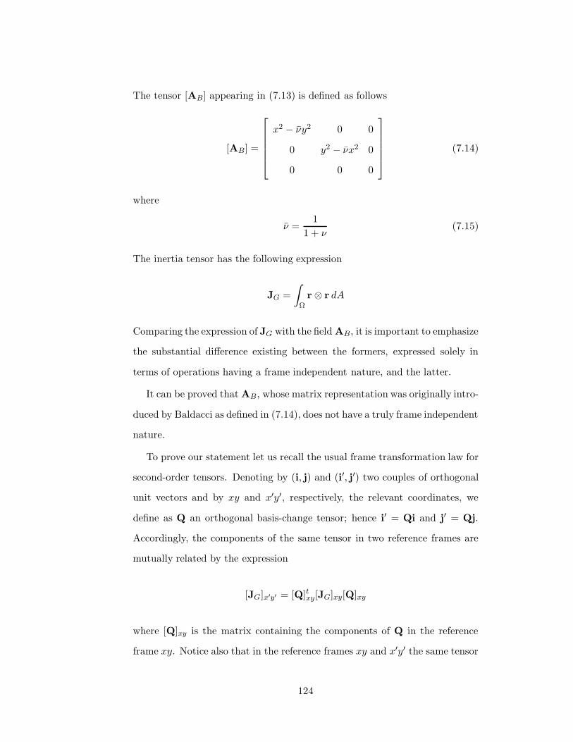
The tensor [AB] appearing in (7.13) is defined as follows

[AB] =

x2 − νy2 0 0

0 y2 − νx2 0

0 0 0

(7.14)

where

ν =1

1 + ν(7.15)

The inertia tensor has the following expression

JG =

∫

Ω

r⊗ r dA

Comparing the expression of JG with the field AB, it is important to emphasize

the substantial difference existing between the formers, expressed solely in

terms of operations having a frame independent nature, and the latter.

It can be proved that AB, whose matrix representation was originally intro-

duced by Baldacci as defined in (7.14), does not have a truly frame independent

nature.

To prove our statement let us recall the usual frame transformation law for

second-order tensors. Denoting by (i, j) and (i′, j′) two couples of orthogonal

unit vectors and by xy and x′y′, respectively, the relevant coordinates, we

define as Q an orthogonal basis-change tensor; hence i′ = Qi and j′ = Qj.

Accordingly, the components of the same tensor in two reference frames are

mutually related by the expression

[JG]x′y′ = [Q]txy[JG]xy[Q]xy

where [Q]xy is the matrix containing the components of Q in the reference

frame xy. Notice also that in the reference frames xy and x′y′ the same tensor

124

JG is represented by formally similar matrixes:

[JG]xy =

∫

Ωx2dA

∫

ΩxydA 0

∫

ΩxydA

∫

Ωy2dA 0

0 0 0

[JG]x′y′ =

∫

Ωx′2dA

∫

Ωx′y′dA 0

∫

Ωx′y′dA

∫

Ωy′2dA 0

0 0 0

To summarize, hence, the matrixes [JG]xy and [JG]x′y′ are formally similar

and represent the same tensor.

Conversely, it can be recognized that tensor AB, represented in the frame

xy by the matrix

[AB]xy =

x2 − νy2 0 0

0 y2 − νx2 0

0 0 0

generally differs from the tensor A′

B which is represented in the second frame

x′y′ by the matrix

[AB]x′y′ =

x′2 − νy′2 0 0

0 y′2 − νx′2 0

0 0 0

To recognize this it suffices to ascertain that the matrix representing AB in the

frame x′y′ does not generally coincide with the matrix which represents A′

B

in such frame. Actually, considering for the base-change the rotation around

the z axis of an angle α whose orthogonal matrix is

[Q]xy =

cos α −sin α 0

sin α cos α 0

0 0 1

.

and assuming for simplicity ν = 0, it is immediately recognized that the matrix

125

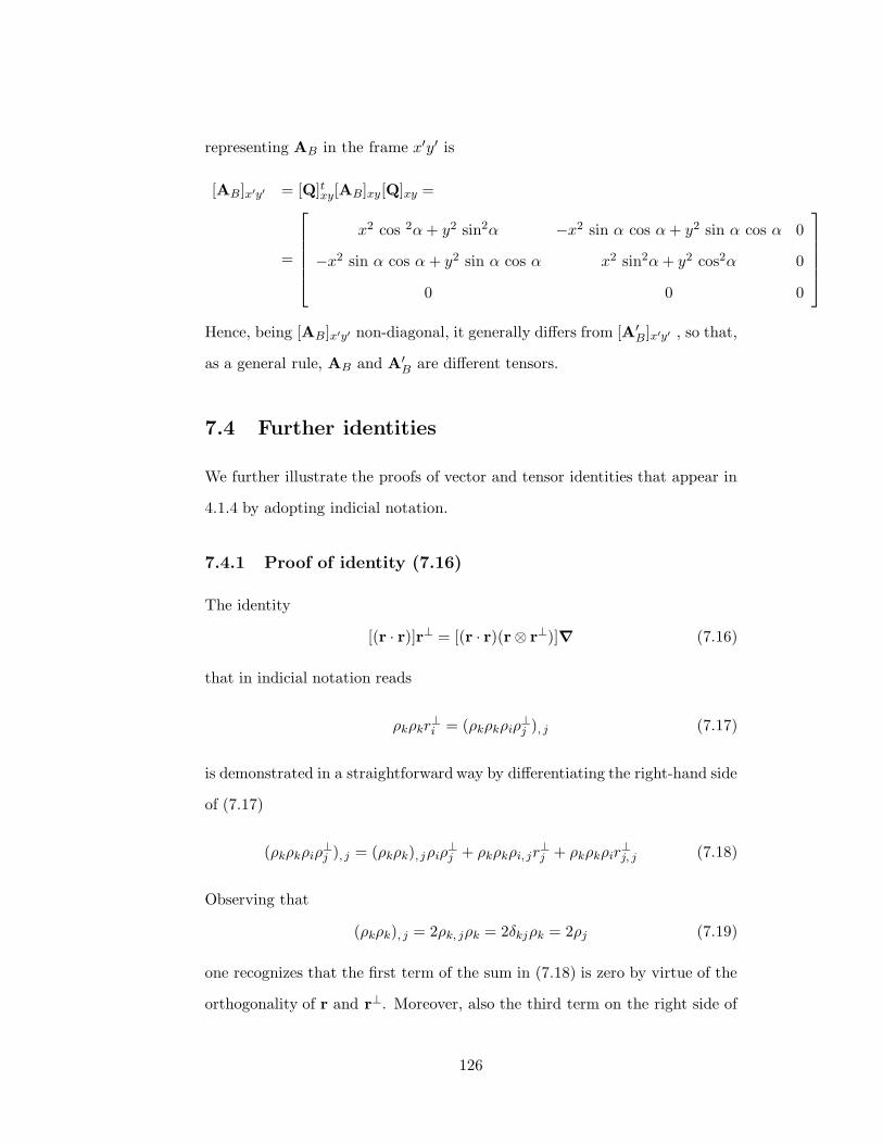
representing AB in the frame x′y′ is

[AB]x′y′ = [Q]txy[AB]xy[Q]xy =

=

x2 cos 2α+ y2 sin2α −x2 sin α cos α+ y2 sin α cos α 0

−x2 sin α cos α + y2 sin α cos α x2 sin2α+ y2 cos2α 0

0 0 0

Hence, being [AB]x′y′ non-diagonal, it generally differs from [A′

B]x′y′ , so that,

as a general rule, AB and A′

B are different tensors.

7.4 Further identities

We further illustrate the proofs of vector and tensor identities that appear in

4.1.4 by adopting indicial notation.

7.4.1 Proof of identity (7.16)

The identity

[(r · r)]r⊥ = [(r · r)(r⊗ r⊥)]∇ (7.16)

that in indicial notation reads

ρkρkr⊥

i = (ρkρkρiρ⊥

j ), j (7.17)

is demonstrated in a straightforward way by differentiating the right-hand side

of (7.17)

(ρkρkρiρ⊥

j ), j = (ρkρk), jρiρ⊥

j + ρkρkρi, jr⊥

j + ρkρkρir⊥

j, j (7.18)

Observing that

(ρkρk), j = 2ρk, jρk = 2δkjρk = 2ρj (7.19)

one recognizes that the first term of the sum in (7.18) is zero by virtue of the

orthogonality of r and r⊥. Moreover, also the third term on the right side of

126

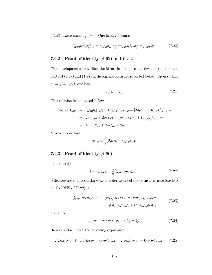
(7.18) is zero since ρ⊥j, j = 0. One finally obtains

(ρkρkρiρ⊥

j ), j = ρkρkρi, jρ⊥

j = ρkρkδijρ⊥

j = ρkρkρ⊥

i (7.20)

7.4.2 Proof of identity (4.92) and (4.92)

The developments providing the identities exploited to develop the counter-

parts of (4.87) and (4.88) in divergence form are reported below. Upon setting

pj = 18(ρhρhρi), one has

pj, kk = ρj (7.21)

This relation is computed below

(ρhρhρi), kk = [(ρhρh), kρi + (ρhρh)ρi, k], k = [2ρkρi + (ρhρh)δik], k =

= 2ρk, kρi + 2ρi, kρk + (ρhρh), kδik + (ρhρh)δik, k =

= 4ρi + 2ρi + 2ρkδik = 8ρi

Moreover one has

pi, k =1

8(2ρkρi + ρhρhδik).

7.4.3 Proof of identity (4.96)

The identity

(ρiρi)ρhρk =1

6[(ρiρi)ρhρkρl], l (7.22)

is demonstrated in a similar way. The derivative of the terms in square brackets

on the RHS of (7.22) is

[(ρiρi)ρhρkρl], l = (ρiρi), lρhρkρl + (ρiρi)ρh, lρkρl+

+(ρiρi)ρhρk, lρl + (ρiρi)ρhρkρl, l

(7.23)

and since

ρi, lρi + ρi, l = δilρi + ρiδil = 2ρl (7.24)

then (7.23) achieves the following expression

2(ρlρl)ρhρk + (ρiρi)ρkρh + (ρiρi)ρhρk + 2(ρiρi)ρhρk = 6(ρiρi)ρhρk . (7.25)

127

7.4.4 Proof of identity (4.97)

On account of (7.24) one has

[(ρiρi)(ρjρj)ρl], l = 2(ρiρi), l(ρjρj) + (ρiρi)(ρjρj)ρl, l =

= 2(ρiρi), l(ρjρj) + 2(ρiρi)(ρjρj)(7.26)

and hence the result

(ρpρp)(ρqρq)δhk =1

6[(ρpρp)(ρqρq)ρlδhk], l . (7.27)

128

7.5 Nomenclature

A cross-sectional area

G centroid of the cross-section domain

J tensor of inertia

l cylinder length

M,Mt bending couple and torque

T, N shear force and normal force

x, y, z Cartesian coordinates

i, j, k unit vectors

σ, ε longitudinal stress and elongation

E Young’s modulus

G tangential elasticity modulus

ν Poisson’s ratio

n unit outward normal to the cylinder boundary

S,E stress and strain tensors

r,u position and displacement vectors

p,u position and displacement vectors restricted to the cross-section plane

Ds shear deformability tensor

129

130

Bibliography

[1] Ahner F, Integral equations and the interior Dirichlet potential problem.

Department of Mathematics, Vanderbilt University, 1976.

[2] Antman S, The principle of virtual work and integral laws of motion.

Arch. Rat Mech. Anal., Vol.69, pag. 231-262, 1979.

[3] Antman S, Nonlinear Problems of Elasticity, Springer Verlag, 1995.

[4] Barre de Saint Venant A J C, Memoire sur la Torsion des Prismes. Mem-

oire des Savants etrangers. vol 14, 223-560, 1855.

[5] Barre de Saint Venant A J C, Memoire sur la Flexion des Prismes. Journal

de Mathematiques de Liuoville Ser. II vol 1, 89-189, 1856.

[6] Baldacci F, Scienza delle Costruzioni. vol I, UTET, 1970.

[7] Baldacci F, Soluzione Generale Diretta del Problema di Saint Venant.

Giornale del Genio Civile, vol 95,759, 1957.

[8] Banerjee P K, Butterfield R, Boundary Element Methods in Engineering

Science, McGraw-Hill, (1980).

[9] Beltrami E, Osservazioni sulla nota precedente, Atti Accad. Lincei Rend.

(5) 1, 141 142, 1892.

[10] Benveniste Y., Chen, T., The Saint-Venant torsion of a circular bar con-

sisting of a composite cylinder assemblage with cylindrically orthotropic

131

constituents. International Journal of Solids and Structures, 40(25), 7093-

7107, 2003.

[11] Benvenuto E, La Scienza delle Costruzioni ed il suo Svilupo Storico. vol

3, Pitagora, Bologna, 1981.

[12] Bisegna P, The Saint-Venant Problem for Monoclinic Piezoelectric Cylin-

ders. ZAMM - Journal of Applied Mathematics and Mechanics, 78(3),

147-165, 1999.

[13] Bobbio S, Electrodinamycs of Materials: Forces, Stresses and Energies in

Solids and Fluids, Accademic Press, 2000.

[14] Bowen R M, Wang C C, Introduction to Vectors and Tensors, Vol.I,

Plenum, 1976.

[15] Brebbia A C, Walker S, Boundary Element Techniques in Engineering,

Newnes-Butterworths, (1980).

[16] Cesaro E, Sulle formule del Volterra, fondamentali nella teoria delle dis-

torsioni elastiche. Rend. Napoli (3a) 12, 311 321, 1906.

[17] Clebsch A, Theorie der Elasticitat der fester Korper. Leipzig, 1862.

[18] Cowper G, The shear coefficient in Timoshenko’ s beam theory. J. Appl.

Mech., 33, 335 340, 1966

[19] Del Piero G: Some properties of the set of fourth-order tensors with ap-

plication to elasticity, J. Elasticity, 3, 245-261, 1979.

[20] De Vivo L, Rosati L, Ultimate strenght analysis of reinforced concrete

sections subject to axial force and biaxial bending Comput. Methods Appl.

Eng., 166, 261-287, 1998.

[21] Dieudonne J Foundations of Modern Analysis, Academic Press, 1969.

132

[22] Dong S.B., Alpdogan, C., Taciroglu, E. Much ado about shear correc-

tion factors in Timoshenko beam theory. International Journal of Solids

and Structures, 47(13), 1651-1665, 2010.

[23] Franciosi V, Fondamenti di Scienza delle Costruzioni. Liguori, Napoli,

1997.

[24] Gibbs J, Wilson E, Vector Analysis. Yale Univ. Press, 1901.

[25] Gibbs J W, Scientific Papers. Vol. 2, Longman, 1906.

[26] Granger R A, Fluid Mechanics. Wiley, 1995.

[27] Gruttmann F, Sauer R, Wagner W, Shear correction factors in Timo-

shenko’s beam for arbitrary cross-sections Computational Mechanics vol

27, 199-207, 2001.

[28] Gurtin M, The linear Theory of Elasticity., in S. Flugge, Handbuch der

Physik, Band VIa/2,Springer, 1972.

[29] Gurtin M, An introduction to Continuum Mechanics., Academic Press,

New York, 1981.

[30] Hamilton W R, On Quaternions or on a New System of Imaginaries in

Algebra., Phil. Mag., iii, 291-302, 1847.

[31] Itskov M, Aksel N, A Closed-Form Representation for the Derivative of

Non-Simmetric Tensor Power Series.Int. Journ. of Solid Struct., 2002

[32] Jaunzemis W, Continuum Mechanics. MacMillan, 1967.

[33] Kim P, Choi U J, Two trigonometric quadrature formulae for evaluating

hypersingular integrals, International Journal for Numerical Methods in

Engineering, vol. 56, 469-486 (2003).

133

[34] Kosmatka J, Flexure-torsion behavior of prismatic beams, part 1: Section

properties via power series. AIAA J., 31, 170 179, 1993.

[35] Lacarbonara W., Paolone A., On solution strategies to Saint-Venant prob-

lem. Journal of Computational and Applied Mathematics, 206, 473- 497,

2007.

[36] Love E, A treatise on the mathematical theory of elasticity. Dover, New

York, 1944

[37] Lubarda A V, Elastoplasticity Theory, CRC Press, 2002.

[38] Malvern E, Introduction to The Mechanics of a Continuos Medium.

Prentice-Hall, New Jersey, 1969.

[39] Mase W, Continuum Mechanics. Schaum’s Outline Series, McGraw Hill,

1970.

[40] Michell J, On the direct determination of stress in an elastic solid, with

applications to the theory of plates. Proc. Lond. Math. Soc. 31,100 124,

1899.

[41] Palazzo V, Rosati L, Valoroso N, Solution procedures for J3 plasticity

and viscoplasticity, Comp. Meth. Appl. Mech. Engrg., 191, 903-939, 2001.

[42] Petrolo A S, Casciaro R, 3D beam element based on Saint Venant’s rod

theory. Computers and Structures vol 82, 2471 2481 , 2004.

[43] Redzi‘c W R, The operator∇ in orthogonal curvilinear coordinates., Eur.

J. Phys., 22, 595-599, 2001.

[44] Renton J D , Generalized beam theory applied to shear stiffness. Inter-

national Journal of Solids and Structures, 27(15), 1955-1967, 1991.

134

[45] Renton J D , A note on the form of the shear coefficient. International

Journal of Solids and Structures, 34(14), 1681-1685, 1997.

[46] Rivlin R, Further remarks on the stress-deformation relations for isotropic

materials, J. Rat. Mech. Anal., 4, 681-701.

[47] Romano G, Romano M, Sulla deformabilita a taglio delle travi di pareti

sottile. Atti dell’ Istituto di Scienza delle Costruzioni della Facolta di

Ingegneria dell’ Universita di Napoli, N. 312, 1983.

[48] Romano G, Rosati L, Sul calcolo delle travi in parete sottile deformabili

a taglio. Nel cinquantenario della facolta di architettura di Napoli Franco

Jossa e la sua opera, 1988.

[49] Romano G, Rosati L, Ferro G, Shear deformability of thin-walled beams

with arbitrary cross sections. International Journal for numerical methods

in engineering, vol 35, 283 306 , 1992.

[50] Rosati L, A novel approach to the solution of the tensor equation AX +

XA = H Int. J. of Solids and Struct., 37, 3457-3477, 2000.

[51] Rosati L, Serpieri R, A Novel Derivation of Beltrami-Michell Compatibil-

ity Equations. Symp. on Trends of Math. to Mech., Maiori, 2002.

[52] Rosati L, Serpieri R, Un approccio di tipo ‘boundary element free’ per

lo studio della torsione di travi con sezione retta poligonale. Associ-

azione Italiana per l’ Analisi delle Sollecitazioni (AIAS) XXXVI Convegno

Nazionale, 4-8 Settembre 2007.

[53] Sapountzakis E J, Mokos V G, A BEM solution to transverse shear load-

ing of beams. International Journal for numerical methods in engineering,

vol 35, 283 306 , 1992.

135

[54] Schramm U, Rubenchik V, Pilkey W D, Beam stiffness matrix based on

the elasticity equations. International journal for numerical methods in

engineering vol 40, 211 232 , 1997.

[55] Serpieri R, Sull’uso delle equazioni di Beltrami-Michell nella derivazione

del modello di trave, Tesi di laurea, Universita di Napoli Federico II, 2002.

[56] Sokolnikoff I, Mathematical Theory of Elasticity. McGraw-Hill, 1956.

[57] Timoshenko S P, Goodier J N, Theory of elasticity. McGraw Hill, 1970.

[58] Timoshenko S, Strength of materials. 3rd edn, D. van Nostrand, New

York, 1958.

[59] Truesdell C , W. Noll: The Non-Linear Field Theories of Mechanics, in

S.Flugge, ed. ’Handbuch der Physik’, vol. III/3 Springer, Berlin 1972.

[60] Viola E, Scienza delle costruzioni. vol 3, Pitagora, Bologna, 1981.

[61] Zieniuk E, Potential problems with polygonal boundaries by a BEM with

parametric linear functions, Engineering Analysis with Boundary Ele-

ments, vol. 25, 185-190 (2001).

[62] Zieniuk E, A new integral identity for potential polygonal domain prob-

lems described by parametric linear functions, Engineering Analysis with

Boundary Elements, vol. 26, no.10, 897-904 (2002).

[63] Zienkiewicz O C, Taylor R L The Finite Element Method, 5th ed.

Butterworth-Heinemann: London, 2000.

136