A statistical verification of a ten year series of ...
206
A STATISTICAL VERIFICATION OF A TEN YEAR SERIES OF COMPUTED SURFACE WIND CONDITIONS OVER THE NORTHE PACIFIC AND NORTH ATLANTIC OCEANS Sigurd Er ing Larson
Transcript of A statistical verification of a ten year series of ...

A STATISTICAL VERIFICATIONOF A TEN YEAR SERIES OF COMPUTEDSURFACE WIND CONDITIONS OVER THE
NORTHE PACIFIC AND NORTH ATLANTIC OCEANS
Sigurd Er
1
ing Larson

Library
vaval Postgraduate Schoo
Monterey. CaWorma 93940

NAVAL POSTGRADUATE SCHOOL
Monterey, California
TA Statistical Verification
of a Ten Year Series of ComputedSurface Wind Conditions Over the
North Pacific and North Atlantic Oceans
by
Sigurd Erling Larson
December 1974
Thesis Advisor: Glenn H. Jung
Approved for public release; distribution unlimited.
U 164892


UNCLASSIFIEDSECURITY CLASSIFICATION OF THIS PAGE (When Date Entered)
REPORT DOCUMENTATION PAGE READ INSTRUCTIONSBEFORE COMPLETING FORM
1. REPORT NUMBER 2. GOVT ACCESSION NO. 3. RECIPIENT'S CATALOG NUMBER
4. TITLE (and Subtitle)
A Statistical Verification of a TenYear Time Series of Computed SurfaceWind Conditions Over the North Pacificand North Atlantic Oceans
5. TYPE OF REPORT A PERIOD COVERED
Master's ThesisDecember 1974
S. PERFORMING ORG. REPORT NUMBER
7. AUTHOHf.j
Sigurd Erling Larson
B. CONTRACT OR GRANT NUMBERfaJ
9. PERFORMING ORGANIZATION NAME AND ADDRESS
Naval Postgraduate SchoolMonterey, CA 93940
10. PROGRAM ELEMENT. PROJECT, TASKAREA * WORK UNIT NUMBERS
II. CONTROLLING OFFICE NAME AND ADDRESS
Naval Postgraduate SchoolMonterey, CA 93940
12. REPORT OATE
December 197413. NUMBER OF PAGES
14. MONITORING AGENCY NAME 6. AOORESS(ll dltterent lrom Controlling Ottice) IS. SECURITY CLASS, (ot Ma report)
Unclassi f iedIS*. DECLASSIFICATION/OOWNGRAD1NG
SCHEDULE
16. DISTRIBUTION STATEMENT (at Ma Report)
Approved for public release; distribution unlimited.
17. DISTRIBUTION STATEMENT (of thm abttract entered in Block 20, il dltterent from Rmport)
18. SUPPLEMENTARY NOTES
19. KEY WORDS (Continue on reverie tide II neceeeary end Identity by block number)
Quas
i
-Geostrophi c Wind North Pacific OceanComputer Model North Atlantic OceanClimatology Ocean Station ObservationsSynoptic Scale Ten Year Trend
20. ABSTRACT (Continue on revert* elde It neceeemry end Identity by block number,)
The increasing interest in long term (inter-annual) weatherchanges and their relation to processes in the ocean is beginningto illuminate the need for and the lack of long term records ofphysically significant variables which occur over the vast oceanicregions of the northern hemisphere. An attempt is made here to
evaluate the accuracy of a hindcast time series of surface wind
1
DD ,^:M„ 1473 EDITION OF 1 NOV 65 IS OBSOLETE
S/N 0101-014-6801!
UNCLASSIFIEDSECURITY CLASSIFICATION OF THIS PAGE (When Dete Entered)


UNCLASSIFIEDCliCU«*»TY CLASSIFICATION OF THIS P«GEW«n D»r. Ent»r«rf:.
20. Abstractvector components and speeds for the period of January 1960through December 1969.
The quasi -geostrophi c model used to calculate these recordsis described as well as the twelve-hourly surface pressure datawhich were used as input. The central moments of the probabilitydistributions of the computed records are compared to those ofcorresponding time series observed on Ocean Station Vessels.Linear correlation coefficients between observations and computedrecords were found to average 0.81 for the components of the windvector and 0.65 for the wind speed. Regression relationsbetween computed and observed records also are presented.Spectral analysis of low pass filtered records showed coherencebetween observed and computed records increased with decreasingfrequency. The accuracy of the computed records in low latitudesalso is estimated.
19. Key Words
Frequency DistributionSpectraCorrel ationRegress i on
DD 1473Form. 1 Jan 73
S/N 0102-014-6601
(BACK)UNCLASSIFIED
SECURITY CLASSIFICATION OF THIS PHOtflWl" Dmlm Lnffd)


A Statistical Verification of a Ten Year
Series of Computed Surface Wind Conditions
Over the North Pacific and North Atlantic Oceans
by
Sigurd Erl ing^LarsonEnvironmental Predi ction 'Research Facility
B.S., University of Washington, 1968
Submitted in partial fulfillment of therequirements for the degree of
MASTER OF SCIENCE IN OCEANOGRAPHY
from the
NAVAL POSTGRADUATE SCHOOLDecember 1974


Library
2aVa> Pos^aduate School
Monterey, California 9
ABSTRACT
The increasing interest in long term (inter-annual)
weather changes and their relation to processes in the ocean
is beginning to illuminate the need for and the lack of long
term records of physically significant variables which occur
over the vast oceanic regions of the northern hemisphere.
An attempt is made here to evaluate the accuracy of a hind
cast time series of surface wind vector components and speeds
for the period of January 1960 through December 1969.
The quasi -geostrophi c model used to calculate these
records is described as well as the twelve-hourly surface
pressure data which were used as input. The central moments
of the probability distributions of the computed records are
compared to those of corresponding time series observed on
Ocean Station Vessels. Linear correlation coefficients
between observed and computed records were found to average
0.81 for the components of the wind vector and 0.65 for the
wind speed. Regression relations between computed and
observed records also are presented. Spectral analysis of
low pass filtered records showed coherence between observed
and computed records increased with decreasing frequency.
The accuracy of the computed records in low latitudes also is
estimated .


TABLE OF CONTENTS
I. INTRODUCTION 12
A. GENERAL 12
B. OBJECTIVES - 14
II. APPROACH - 15
A. THEORETICAL BACKGROUND 15
1. Geostrophic Wind Equation 15
2. Surface Wind - Geostrophic Wind Relation --17
B. THE METHOD OF COMPUTING THE SURFACE WIND 18
C. DATA GENERATION 22
1. Input Data for the Model 22
2. Observational Data 24
3. Data Used for Analysis 24
D. DATA CONDITIONING 25
1. Gaps and Gross Error Elimination 25
2. Filtering -26
III. RESULTS - -- ---28
A. ENSEMBLE ANALYSIS - --- --28
1. Central Moments 28
a. Wind Speed 29
b. Zonal Component 33
c. Meridional Component 34
2. Ten Year Trend 37
3. Correlation and Regression Analysis 40
4. Error Analysis 46


a. Separation Distance 46
b. Friction in Low Latitudes 47
B. SPECTRAL ANALYSIS - - 49
1. Autocorrelation 49
2. Energy Density 51
3. Coherence and Phase 53
IV. SUMMARY -- 57
A. ACCURACY OF THE MODEL 57
B. POSSIBLE APPLICATIONS 58
LIST OF REFERENCES 97
INITIAL DISTRIBUTION LIST -- 99


LIST OF TABLES
I. Monthly distribution of surface pressure analyses.The number of analyses used is in the numerator,and the denominator equals the number of twelvehour intervals in the month 59
II. Positions of the Ocean Stations, computationalgrid points and the distance between them 60
III. Central moments and figures of merit (FM) of thedistribution of observed and computed (C) windspeeds for each Ocean Station 61
IV. Central moments and figures of merit (FM) of thedistribution of observed and computed (C) zonalcomponents for each Ocean Station 62
V. Central moments and figures of merit (FM) of thedistribution of observed and computed (C)meridional components for each Ocean Station 63
VI. Linear correlation coefficient (R) and coefficientof determination (R2) between observed and computedtime series for each Ocean Station 64
VII. Coefficients for regression of computed time serieson observed time series for each Ocean Station 65
VIII. Coefficients for regression of observed time serieson computed time series for each Ocean Station 66
IX. Scatter diagram symbols (for Figures 11 and 12)and the corresponding number of coincident computedand observed wind speed pairs 67
X. Ratio of surface wind speed (Vs) to geostrophicwind speed (Vg) and deflection angle (in degrees)at low latitudes as tabulated by Brummer, e_t al .
and as formulated in the model 67
XI. Autocorrelation of observed and computed timeseries at Ocean Station Bravo and Ocean StationVictor at selected frequencies 68
2 - 2XII. Energy density (in m sec ) of observed and
computed time series for Ocean Station Bravo andOcean Station Victor at selected frequencies 69


XIII
XIV.
Coherence between observed and computed timeseries for Ocean Station Bravo and Ocean StationVictor at selected frequencies
Phase difference (in degrees) between observedand computed time series for Ocean Station Bravoand Ocean Station Victor at selected frequencies
70
- 70

LIST OF FIGURES
1. Latitude dependence of the ratio of the surface windspeed (Vs) to the geostrophic wind speed (Vg) asfound by Roll (broken line), Carstensen (solid line)and as formulated in the model (dashed line) 71
2. Latitude dependence of the deflection angle forvarious wind speeds (W in m sec-1) as formulatedin the model 72
3. Latitude dependence of the deflection angle as foundby Roll (broken line), Carstensen (solid line), andas formulated in the model for wind speeds (W) of5 m sec -
! and 15 m sec -! (dashed lines) 73
4. Result of five point binomial filter applied to a
typical portion of a zonal component time series.Original series (solid line) and filtered series(dashed line) are shown in the upper graph. Theresidual series is shown in the lower graph 74
5. Central moments of the distributions of observed(solid line) and computed (dashed line) wind speeds.(Mean wind speed in m sec-1; variance in m^ sec"^) --75
6. Central moments of the distribution of observed(solid line) and computed (dashed line) zonalcomponents. (Mean zonal component in m sec-1;variance in m2 sec-2) 76
7. Central moments of the distributions observed(solid line) and computed (dashed line) meridionalcomponents. (Mean meridional component in m sec-1;variance in m 2 sec-2.) 77
8. Total change (integrated linear trend) over theten year period from January 1960 through December1969 in the observed (solid line) and computed(dashed line) wind speed and zonal and meridionalcomponents (in m sec"l) 78
9. Regression relations between the observed andcomputed wind speeds for Ocean Station Juliet 79
10. Regression relations between computed wind speedsfor Ocean Station November 80
11. Scatter of observed and computed wind speeds(in m sec-1) a t Ocean Station Juliet. Table IX
defines the symbols 81


12.
13
14.
15.
16.
17.
18.
19.
20.
21 .
22.
23.
24.
25.
26.
Scatter of observed and computed wind speeds(in m sec-1) at Ocean Station November. Table IXdefines the symbols
Mean error (in m sec" ) dependence on separationdistance for wind speed and the zonal and meridionalcomponents. Estimated best-fit lines are shownfor components
Linear correlation coefficient (R)
.
dependence onseparation distance for wind speed and the zonaland meridional components
Autocorrelation of observed (CO) and computedwind speeds at Ocean Station Bravo
Autocorrelation of observed (CO) and computedwind speeds at Ocean Station Victor
Autocorrelation of observed (CO) and computedzonal components at Ocean Station Bravo
Autocorrelation of observed (CO) and computedzonal components at Ocean Station Victor
Autocorrelation of observed (CO) and computedmeridional components at Ocean Station Bravo
Autocorrelation of observed (CO) and computedmeridional components at Ocean Station Victor --
2 -2Log energy density (in m sec ), coherence, andphase difference (in degrees) for computed andobserved wind speeds at Ocean Station Bravo
XX)
XX)
XX)
XX)
XX)
XX)
2 - 2Log energy density in (m sec ), coherence, andphase difference (in degrees) for computed andobserved wind speeds at Ocean Station Victor —
82
83
84
85
86
87
88
89
90
91
92
2 - 2Log energy dens i ty (in m sec ), coherence, andphase difference (in degrees) for computed andobserved zonal components at Ocean Station Bravo 93
2 - 2Log energy density (in m sec ), coherence, andphase difference for computed and observed zonalcomponents at Ocean Station Victor 94
2 -2Log energy density (in m sec ), coherence, andphase difference for computed and observed meridionalcomponents at Ocean Station Bravo 95
2 - 2Log energy density in m sec ), coherence andphase differences for computed and observed meridionalcomponents at Ocean Station Victor 96
10


ACKNOWLEDGMENTS
The author wishes to express his gratitude to the Church
Computer Center, Naval Postgraduate School; to Fleet Numerical
Weather Central for use of their computers and surface
pressure data; to David Husby, National Marine Fisheries
Service, for use of Ocean Station observational data; to
Andrew Bakun, National Marine Fisheries Service for valuable
contributions to the formulation of the model; to Dean Dale,
Fleet Numerical Weather Central, for a critical review of the
model; to Robert Baily, formerly with the Environmental
Prediction Research Facility, for his highly competent manage-
ment of many of the computer runs required; to Professor
Edward Thornton who generously provided his spectral analysis
program and much valued assistance in its use; and especially
to Professor Glenn Jung, faculty advisor, for his patient
guidance throughout what must have seemed an interminable
undertaking.
11


I INTRODUCTION
A. GENERAL
One of the most important variables encountered in the
study of physical oceanography and air-sea interaction is
the wind field at the sea surface. To a large degree, the
surface wind velocity and its variability, both in time and
space, determine the exchange of heat and momentum across
the air-sea interface. Through such exchange the wind affects
not only oceanic surface phenomena, such as waves and surface
currents, but also features within the sea such as the
vertical thermal structure and deep currents.
The smallest scale of concern in this study is the
synoptic scale. Such a scale covers a period of time from
several hours to several days and a distance from several
tens of kilometers to several hundred kilometers. Past
attempts at estimating the surface wind field on this scale
have been of two types. One could either average wind obser-
vations collected over a given area for a specified period
of time (Seckel, 1970) or one could estimate the surface winds
from a similar collection of observations of other variables,
such as surface atmospheric pressure (Roden, 1974).
The accuracy of synoptic scale surface wind fields
derived directly from wind observations suffers from two
major drawbacks: a paucity of observations, and the high
variability of the small scale wind field. The small number
12


of observations usually available in a typical mid-ocean
region over a three-or-four-day period are very often grouped
together in a small section of the region, often along major
shipping lanes or along the track of a single ship. In
addition, major portions of the open ocean lack any reports
of wind conditions for weeks at a time. As a result, the
few reports available must necessarily be used to describe
large areas when estimating the synoptic scale wind field.
Verploegh (1967) found, however, that simultaneous wind speed
observations from ships less than sixty miles apart in
"synopti cal ly homogeneous areas" differed significantly. His
analysis indicated the correlation coefficient between such
observations was less than 0.7.
Because of such considerations, the second, indirect
approach is generally used to estimate the synoptic scale
surface wind field. This approach depends on the fact that
the distribution of surface atmospheric pressure can be more
accurately described than can the surface wind field from a
limited number of observations, due to the lower variability
in time and space of the surface atmospheric pressure field.
An accurate estimate of the synoptic-scale surface wind field
may be made by applying the geostrophic approximation to the
surface atmospheric pressure field.
13


B. OBJECTIVES
Although the relation of the geostrophic to observed
wind is a popular topic, this study is not intended to be a
detailed examination of that relation. Rather, it is limited
to an evaluation of one particular surface wind model used,
in this study, to hindcast time series of surface winds over
oceanic areas. The model is quasi -geostrophi c , incorporating
the effects of friction. It is one part of operational
oceanographi c models used at Fleet Numerical Weather Central
and at Fleet Weather Central, Rota (Spain).
As a result of this study, the ten-year average and
linear trend of observed wind conditions at several points
in the North Atlantic and North Pacific Oceans were determined
and compared to those calculated from the model. The primary
objective of the study was however, to determine the accuracy
of the computed time series and to determine if calibration
factors could be applied directly to them in order to increase
their accuracy.
The model was developed by the author while at FleetNumerical Weather Central; most of the work of this study wascarried out while the author was at the Environmental PredictionResearch Facility.
14


II. APPROACH
A. THEORETICAL BACKGROUND
1 . The Geostrophi c Wind Equation
Geostrophic wind has been considered to be an
acceptable estimate of the true surface wind in many studies
of oceanography and air-sea interaction (Roden p_£. cvt . ,
Namias, 1963). Geostrophy assumes a balance between the
pressure gradient force and the Coriolis force and ignores
acceleration, friction, and vertical motion. This balance is
gi ven in equation CO:
V n= k X -If v
HP
g pf H(1)
where V = geostrophic wind vector
P = surface pressure
v u= — i + — j (horizontal gradient operator)
n o X ay
X = vector product operator
f = 2oj sin (the Coriolis parameter)
u = angular rotation of the earth
= latitude
p = ai r densi ty
k = unit vertical vector
Although this approximation is widely used, its accuracy is
limited by the required assumptions indicated above.
15


The true surface wind vector is the resultant of
the geostrophic wind vector and an ageostrophic wind vector.
The direction and magnitude of the ageostrophic wind vector
determines the accuracy of the geostrophic approximation.
Unfortunately the ageostrophic vector has been shown to vary
significantly over the Northern Hemisphere (Roll, 1965;
Carstensen, 1967; Brummer, e_t aj_. , 1974). Such variability
makes the geostrophic wind hard to relate to the surface wind
in studies on synoptic or larger scales.
The accuracy of the geostrophic approximation is
also limited, in practical application, by the temporal
variability of the surface pressure field. In practice, the
geostrophic approximation is often applied to surface pressure
distributions averaged over a month or more (Namias, op cj_t . )
.
Such a procedure results in calculating the vector resultant
of the geostrophic wind for the averaging period. Obviously,
non-conservative phenomena which depend on the surface wind
cannot be treated using such a resultant wind field. In the
study of such phenomena, the resultant vector is assumed to
represent the mean or steady-state wind prevailing over the
averaging interval.
Whether or not the resultant wind is a good esti-
mate of the mean wind depends on the variance of the wind
vector over that interval. The mean wind speed, WM , and the
resultant wind speed, WR
are given below in terms of components
16


w
T
E
t=l
(u2
tv2
t)
:
„ - ^—
~
(2)
(3)
where U., V. are orthogonal components of the wind vector at
time t for 1 <_ t <_ T . (Averaging twelve hourly data over
thirty days, we have 1 <_ t <_ 60). The difference between
2 2WM
and WR
can be expressed in terms of the variance of each
2 2 2of the components, a and a , and of the wind speed, a ;
u 2 „2 2,2 2WM " W
R= % + a
v" a
w(4)
whereT II* ( 1 uA 2
t=i ' yt=i '
y
(5)
2 2and similarly for a , and a . As will be shown in Section
III-A, the difference expressed in equation (4) results in
a drastic under-estimate of wind speed when the resultant
wind is used in place of the mean wind speed in problems
involving the square of the wind speed.
2 . The Surface Wind-Geostrophic Mind Relation
Although this is not a study of the general relation
of the geostrophic wind to the surface wind, a few words
regarding this relation are appropriate for background. As
indicated, the surface wind vector can be resolved into
17


geostrophic and ageostrophi c components. The ageostrophic
component can be assumed to consist of a frictional component
and an acceleration component (Briimmer, e_t aj_. , op ci t . )
.
The frictional component is generally accepted as
the dominant ageostrophic component (Verploegh, op c i t .
,
Brummer, et a]_. , op c i t . ) . Haltiner and Martin (1957) suggest
that the frictional component is dependent on the stability
of the surface layer of the atmosphere. Hasse (1974) has
demonstrated that the dependence of the surface wind speed on
the surface pressure gradient is an order of magnitude greater
than its dependence on stability.
The effects of stability have not been explicitly
incorporated into the model; to some degree however, they
have been implicitly incorporated through the latitude
dependence of terms in the various equations of the model.
The major effects of stability are assumed to occur in the
region between 45°N and 25°N. This implicit incorporation of
stability is shown in the ratio of the surface wind speed to
the geostrophic wind speed in Figure 1.
B. METHOD OF COMPUTING THE SURFACE WIND
The calculations were performed on the Fleet Numerical
Weather Central (FNWC) 63x63 polar stereograph ic grid of the
northern hemisphere (FNWC, 1974). On this square grid the
equator is an inscribed circle, i.e., tangent to the grid
18


boundary. The grid mesh length at 60°N is 381 km and increases
with increasing latitude. The data, although calculated on a
polar stereographic grid, will be discussed relative to a
2Mercator grid.
The components of the horizontal pressure gradient at a
given grid point (i,j), were approximated to the second order
by equation (6):
where K1
|| (i j) = MLLLilKl {P(i-2,j) - K
2[p(i-i,j)
- P(i+l,j)] - P(1+2,j)}
1/12
8
(6)
MF(i,j)
= 381 km (mesh length)
1+SIN(60°) , . , .. . , .
=i + c t m ) a \
— = ma P factor of the grid at
point (i ,j)
= latitude of grid point ( i , j ) ,
g pand similarly for ry(i,j). Using (1) with a constant air
- 3 - 3density of 1.22 x 10 gm cm , the geostrophic wind vector
Both Mercator and polar stereographic projections areconformal projections of the earth and as a result, anglesare preserved when transformed from one to the other (Taylor,1955).
19


at each point was found. The magnitude of this vector (the
geostrophic wind speed) was then reduced as a function of the
latitude of the grid point according to (7):
Vs(i,j) = A [B(0)] V
g(i,j) (7)
where V (i,j) = surface wind speed at grid point (i,j)
V ( i , j ) = geostrophic wind speed at grid point (i,j)
A = 0.93 4
(0.65+0.2(0/25°) ; < 25°
B(0) =<0.85 ; 25° < < 45°
(o. 75 + 0.1 ^ 9^;^ ; 45° <
The resulting ratio of (V /V ), which is strongly
dependent on latitude, was suggested by data from Roll
( op ci t . ) and Carstensen (op_ c i t . ) . The value of (V /V )
used in the model is plotted in Figure 1 along with values
The sine function, SILA, used in the calculation of theCoriolis parameter for the geostrophic wind calculation andin the calculation of the deflection angle (equations 1 and8) was modified below 35°N. This was done in an attempt toreduce the impact of this parameter in the calculation ofequatorial winds. The modification was suggested by thesubroutine SNLTSRX in the Fleet Numerical Weather Centralprogram 1
i
brary . ( FNWC , op c i t . ) . The value of SILA south of3 5° N is given by the tangent to the sine curve at 3 5 ° N , i.e.,SILA(0) - 0.0144(SIN-1 (0) ) + 0.075 for <_35°.
4The factor A resulted from erroneously using 408 km
for the grid mesh length in the model (D. Dale, FNWC,personal communication).
20


found by Roll and by Carstensen. Although Carstensen derived
his relation from a much smaller data set than that in Roll's
study, the major features of the latitude dependence are
similar. The value of (V /V ) used in the present models 9
attempts to reproduce the first order dependence on latitude:
i.e., the maximum in the mid-latitudes, sharply decreasing
with decreasing latitude toward the equator and a more modest
decrease with increasing latitude above 45°N.
After being reduced in speed, the surface wind vector
is then rotated to the left of the geostrophic wind vector
(toward low pressure). Together, deflection and reduction
of the geostrophic wind vector simulate the effects of friction
(Haltiner and Martin, op c i t . ) . The deflection angle, a, was
cal cul ated from (8)
:
a = K1
(K2
- K3V^) / (1+SIN 0) (8)
where K-, - 1 .475
K2
= 22.5
K3
= 1 .75 x 10" 2
V = surface wind speed, from (7) .
Figure 2 is a plot of a against latitude for several values
of surface wind speed.
The dependence of a on the square of the surface wind
speed strongly decreases the deflection angle associated with
high surface wind speeds. This approach was based on the
assumption that high winds (associated with well-defined
21


cyclones) generally show less cross-isobar flow than do the
low winds associated with nearly flat surface pressure
distributions. The assumed reduction in the deflection angle
as wind speed increases could be caused by a slight reduction
in the frictional drag experienced at higher values of surface
wind speed. In this model, however, this reduction becomes
significant only at relatively high wind speed. For example,
at 20 m sec" the deflection angle is 75% of its value at
1 rn sec" . At 30 m sec" the deflection angle has been
reduced to 30% of the value at 1 m sec- i
As with the value of (V /V ), the latitude dependence
of m also was suggested by Roll and Carstensen. Figure 3 is
a plot of the value of a against latitude as found by Roll,
by Carstensen, and as used in this model. The values of a
froE the model are those for surface wind speeds of 5 and
15 sec" . Less than 15% of the reported wind speeds in
this study were outside this range. As in the case of the
reduction factor, the expression for a attempted to reproduce
the najor features of the latitude dependence shown by both
Roll's and Carstensen's data.
C. DATA GENERATION
1 . Input Data for the Model
The model was used to calculate a ten-year time
series of the surface winds at twelve hour intervals at grid
poiats near international Ocean Stations. The input for the
model consisted of surface pressure fields on the FNWC grid.
22


All the available surface pressure analyses for synoptic
periods of 0000 GMT and 1200 GMT were used for the ten-year
period from 0000 GMT 1 January 1960 to 1200 GMT 31 December
1969. However, not all the analyses for this period were
available and this required some conditioning of the output
data which will be discussed in Section II-D.
The number of surface pressure analyses used for
each month in the ten-year period are shown in Table I. In
general, the analyses were fairly evenly distributed over
the twelve months. The month of April had the poorest
representation with 488 (81%) of the 600 possible analyses
used, while November was the best represented with 534 (89%)
of the 600 possible analyses. Most of the missing data were
concentrated in the period from April 1960 through June 1962.
Within this period only one analysis per day was available.
As a result, only 365 (50%) of the 730 possible analyses were
used for 1961. The best-represented year was 1967 for which
728 (99.7%) of the 730 possible analyses were available. The
missing analyses totaled 1098 (15%) of the 7306 possible in
the ten-year interval.
According to Bakun (1973), who used the same set
of surface pressure analyses to calculate coastal upwelling
indices, the analyses between January 1960 and July 1962
were from the National Climatic Center at Asheville, North
Carolina. The analyses from July 1962 through December 1969
were produced by objective computer analyses at FNHC.
23


2
.
The Observational Data
The observed wind data were taken at six interna-
tional Ocean Stations (OS). These were the only continuous
time series of observed wind speed and direction available
for the ten years of this study. As these data were assumed
to be of high quality, no attempt was made to determine their
accuracy other than gross error checking as described in
Section 1 1 - D . The observations were thus used as the standard
against which the calculated wind records were verified.
The observed wind speed and direction were extracted
from the Surface Marine Observation Tape Family 11 from the
National Weather Record Center for the following Ocean
Stations: BRAVO (OSB), DELTA (OSD), JULIET (OSJ), PAPA (OSP),
VICTOR (OSV), and NOVEMBER (OSN).5
Table II indicates the
position of each OS, the position of the computational grid
points, and the distance between each OS and its correspond-
ing grid point.
3. Data Used in Analysis
Both the observed and computed data were transformed
to zonal (East-West) and meridional (North-South) components.
The resulting set of three time series for each OS and each
grid point (a total of 39) consisted of the values of zonal
All the Ocean Station records with the exception ofNOVEMBER (OSN) were compared to computational time seriesfrom a single grid point near their location. Time serieswere calculated at two grid points bracketing OSN in orderto estimate the variability of the computed wind over a
single grid mesh length. These computation grid points willbe referred to, henceforth, as NIC and N2C.
24


and meridional components and the wind speed at 0000 GMT and
1200 GMT for the ten-year period from 1 January 1960 to 31
December 1969. It should be noted here that a negative zonal
value indicates a wind from the West and a negative meridional
value indicates a wind from the South.
D. DATA CONDITIONING
1 . Gaps and Gross Errors
A check for gross errors was performed following
extraction and transformation of the observed and computed
wind vectors. A wind speed of 50 m sec" was selected as the
maximum allowable value; this established a gross error
criterion in order to eliminate only those errors caused by
hardware failure such as tape parity. No wind speed values
in excess of 50 m sec" were found in either the computed or
observed data.
After gross error checking was completed, ensemble
analysis was performed on the observed and computed time
series. Following that, the gaps in the records were removed.
The computed records differed markedly frora the observational
data in both the number and length of gaps. For the eighteen
observational records, the number of single point gaps per
record averaged about 200, while about 300 points per record
were missing in gaps of two or more consecutive points. Only
about 150 points per record were missing from the computed
time series in the form of multiple point gaps. However, for
25


these computed records there were about 950 single point
gaps, due primarily to missing pressure analyses within the
period of April 1960 through June 1962.
Because of the high proportion of single missing
data points in the calculated record, a single missing value
was replaced by linear interpolation between the preceding
and following value. For gaps consisting of two or more data
points, the missing data were replaced by the time series
average. This procedure was suggested as a means of filling
gaps while not introducing spurious data into the records
which would be subjected to subsequent spectral analysis.
2. Filtering
Filtering was done on the computed and observed
records in order to allow comparison of records with nearly
equal data content. Because of the substantial missing data
in the high frequency part of the computed record (due to
single point gaps) and because of the stated interest in
large scale phenomena, a low-pass filter was applied to each
of the computed and observed time series after the gaps were
E. Thornton, Dept. of Oceanography, Naval PostgraduateSchool, personal communication.
26


removed. A five-point binomial filter indicated in equation
(9)was used.
Y(t) = s a. • X(t+lAt)i=-2
n(9)
where Y(t)
ai
X(t+iAt)
At
= filtered value at time t
= binomial coefficient (0.38, 0.25, 0.06,for i = 0, + 1 , +2)
= unfiltered value of the time series attime t+iAt
= sample interval (0.5 days)
Figure 4 shows the effect of applying this filter to a typical
segment of one of the computed time series. The amplitude of
the residual series (unfiltered minus filtered) is approxi-
mately the same amplitude as the filtered series, indicating
that approximately 50% of the variance of the unfiltered
series was removed by filtering. This estimate of 50% was
confirmed by a comparison of the filtered and unfiltered record
variance (not shown). Before any filtering or gap removal was
done, however, the observed and computed records were analyzed
as ensembles in order to determine the relation between them.
Such a filter has a frequency response, R(f), atfrequency f ,
R(f) - cos4
(irfAt) (10)(Panofsky and Brier, 1958).
27


III. RESULTS
A. ENSEMBLE ANALYSIS
In this section the ensembles of the observed and
computed data are compared. The term ensemble is taken to
mean the set of values which constitute a given time series
of the variable in question. Due to the length of the records
(ten years), significant questions about short-term accuracy
of the model cannot be treated by ensemble analysis. The
problem of short-term accuracy is investigated through
spectral analysis as reported in Section III-B.
1 . Central Moments
Both the observed and computed data were considered
to have come from specific probability densities. While these
probability densities were not explicitly defined in this
study, they were described by determination of their central
mordents. The general form of the central moment of a given
probability density is given by equation (11).
R
R
N (x.-p)E
i = lN
(11)
where p D = R central moment
1th
R
1value of the variable X
N = total number of values of X in the ensembleN
M = E X . / N
1=1 1
mean value of the ensemble
28


In practice, the third and fourth moments are
normalized by the third and fourth powers of a (a = y? ),
the standard deviation of the ensemble (Tennelces and Lumley,
1972). In this study the first moment is taken to be the
mean rather than zero as in equation (11).
The criterion used to estimate the accuracy of the
computed data - the "figure of merit" - was the ratio of a
central moment of the computed record to that of the observed
record. This simple criterion was intended to show only two
things: the percentage of a given observed statistic present
in the corresponding computed record; and those statistics
which differed in sign between computed and observed records
(resulting in a negative figure of merit).
As the computed data were compared to observationsQ
at six OS, the average figure of merit for the model was
taken to be the average of the figures of merit for each OS.
An average was found also for the three OS in the Pacific and
for the three in the Atlantic,
a. Wind Speed
The values of the central moments and their
figures of merit for the observed and computed wind speed are
o
The two computed records, NCI and NC2, were comparedto the observational record at OSN. In order not to over-emphasize these data when considering averages, the averageof the figures of merit of NC2 and NCI was used as the figureof merit at OSN when calculating the overall average figureof merit or the average of the figures of merit in the Pacific
29


tabulated in Table III and are plotted against latitude in
Figure 5. The average computed wind speed (first moment)
varied between 95% and 91% of the average wind speed observed
at the six OS. Over the latitude range of the OS (30°N to
56.5°N), the average observed wind speed decreased from a
maximum of 10.6 m sec" in the Westerlies (OSP) to 6.6 m sec"
in the North East Trades (OSN) for the ten years between 1960
and 1969. The average figure of merit for the mean computed
wind speed is 0.92. This figure is 0.91 in the Pacific and
0.93 in the Atlantic.
It is worth noting again here that we are
dealing with an average wind speed and not a resultant wind
speed. The resultant wind speed can be determined by
combining the average zonal and meridional components by
vector addition. The average wind speed was determined from
the wind speed at each interval in the ten year time series.
The variance (second moment) of the wind speed
2 -2decreased from approximately 28 m sec in the latitudes of
2 - 2the Westerlies to approximately 10 m sec in the latitudes
of the Trades - a latitude dependence similar to that of the
average wind speed. The average figure of merit for the
variance is 1.07. Only at 0SB is the figure of merit (0.89)
less than unity. The maximum (1.24) is shared by 0SJ and OSN
(NC2). When comparing the variances of the computed and
observed records by means of the F test it becomes apparent
that any figure of merit for the variance which is not equal
30


to unity is statistically significant at the 1% level due to
the very large (>6000) number of degrees of freedom for each
ensemble (Freund, 1962). That is, the probability that the
computed and observed ensembles come from the same probability
density is less than 0.01. Relating these statistically
significant differences in the observed and computed records to
to physical causes is, for the most part, beyond the scope of
this study. However, the location of the grid point NC2
(at 32N) at the northern boundary of the North East Trades
appears associated with the high figure of merit at this
location. Seckel (o_p_ c i
t
. ) suggested the wind speed is much
more variable at 32N (NC2) than it is in the Trades (at OSN),
and thus a figure of merit for wind speed variance greater
than 1.0 is to be expected between these records. This suggests
that the model can resolve significant changes in the varia-
bility of the wind field which occur on a scale of one
gri d-mesh length.
The standard deviation (square root of the
variance) can be used to estimate an upper bound on the
average fluctuation of the wind speed from the ten-year mean.
According to Chebyshev's Inequality, the probability that the
wind speed will differ from the average by more than 1.414
standard deviations is less than 0.50 (Freund, o_p_ c i t . ) . The
value of 1.414 a in the Westerlies was about 7 m sec . Tin's
value is considerably greater than the diurnal range of the
31


wind speed in the open ocean reported by Roll (op c i t . ) .
Thus, most of the variance in the wind speed observed at OS
over the ten-year period was due to variations of a period
longer than twelve hours. The 50% reduction in the variance
due to filtering as indicated in Section II-D-2 suggests that
50% of the variance is due to wind speed fluctuations of a
period greater than two days.
The third moment (skewness) of the computed
wind speed is higher than that of the reported wind speeds
at all the OS. The average figure of merit for all the
locations is 1.30. This high value represents a tendency of
the computed wind speed to exceed reported wind speed
significantly in cases of high wind. Of the locations
studied, this tendency is most pronounced in the Pacific
Trades. The fact that the average figure of merit was greater
than one for the skewness and less than one for the average
of the wind speed suggests that the overestimated high wind
speeds in the computed record were more than compensated by
more numerous underestimati ons of low wind speeds. The
omission of the effects of curvature, i.e., the acceleration
of the wind due to the centrifugal force, in the geostrophic
9equation was suggested as the cause of this effect.
R. Elsberry, Dept. of Meteorology, Naval PostgraduateSchool, personal communication.
32


The exaggeration of both extremely low and
high wind speeds is also suggested by the fourth moment
(kurtosis) which indicates the amount of extreme data in the
enseusble, i.e., the number of data points in the ensemble
whicli are far from the mean. The figure of merit for
kurtosis is highest for the Pacific in the transition from
Westerlies to Trades (OSV and 0SN-NC2). As can be seen in
Figure 5, the value of the kurtosis of the wind speed
increases dramatically in the Trades. However, this increase
is an artifact of the normalization by the fourth power of
the standard deviation, which is much smaller in the Trades
than in the Westerlies, and does not indicate that ^/ery strong
winds occur more frequently in the Trades than in the Westerlies
b. Zonal Component
The first four moments for the zonal component
of the wind vector are shown plotted against latitude in
Figure 6. Their values and figures of merit are tabulated
in Table IV. The latitude dependence of the first moment
(average or resultant) of the observed and computed zonal
components is similar. The difference between the first
moments of the observed and computed zonal components is
greatest at OSP (0.85 m sec" ). While the average figure of
merit of the first moment is 1.0, the model is more accurate
in 1 1. e Atlantic than in the Pacific Ocean. In the Pacific the
figure of merit ranges from 0.43 to 1.45 and averages 1.01.
In the Atlantic the range was smaller, from 0.89 to 1.05,
and the figure of merit averages 0.98.
33


This disparity between Atlantic and Pacific
is evident also when comparing the variance (or second moment)
of the observed zonal component to that of the computed zonal
component. The figure of merit ranges between 0.83 and 0.95
in the Atlantic Ocean and between 0.78 and 1.02 in the
Pacific. Overall, it averages 0.88, indicating that
the model reproduced about 88% of the variance of the zonal
wind. The relatively poor accuracy of the model at 0SP as
shown in Figure 6 is unexplained; however, the poor agreement
between 0SN and grid point NC2 is probably due to the transi-
tion to the Trades as previously suggested.
The skewness showed the poorest agreement of
all the moments calculated for the computed and observed
zonal components. The model consistently underestimated this
parameter; the figure of merit averaged only 0.63. The signs
of the computed and observed skewnesses differed at 0SJ
;
however, the values at this point were so near zero that the
difference is insignificant.
The kurtosis (fourth moment) of the computed
zonal component was consistently higher than that of the
observed zonal component. The average figure of merit was
1.11, and was nearly equal in both the Atlantic and Pacific
Oceans .
c. Meridional Component
The first four moments of the probability
density of the computed and observed meridional components
are tabulated in Table V and are plotted against latitude in
Fi gure 7
.
34


The figure of merit for the mean of the
meridional component, averaged for all locations, was 1.22
and was nearly equal in the Pacific and the Atlantic Oceans.
The individual figures of merit of the means suggest that the
computed meridional component has a bias of 0.3 to 0.9 m sec"
This bias is a fictitious (computed) component from the south,
which reduced the average computed meridional component at
those stations where the resultant direction was from the
north (OSB and OSN); and it increased the meridional component
at those stations where the resultant direction was from the
south. Such a consistent bias suggests that a fictitious
east-west gradient (higher pressure to the east) in the sur-
face pressure analyses may occur over both the Pacific and
Atlantic Oceans.
The variance of the observed and computed
meridional components showed only slightly better agreement
than was the case for the zonal component. Averaged over the
locations studied, the model reproduced 92% of the variance
of the observed meridional component. Again, OSN (NC2)
showed the highest figure of merit due to the effects of the
transition to the Trades.
The skewness of both the observed and computed
values was nearly zero at all locations north of the Trades.
This indicates that, relative to the average meridional
component, the strong positive (northerly) and negative
(southerly) fluctuations were equally distributed. The
35


negative value of the skewness at OSN indicates that the
southerly (relative to the mean) extremes predominated.
Because the skewness was so near zero for all stations north
of the Trades, figures of merit at these locations have little
meaning. In the Trades, the model overestimated the skewness
by up to 98%. This yery high figure of merit is in marked
contrast to that for the skewness of the zonal component
(Table IV). This discrepancy suggests that in the Trades,
extreme values in the calculated record of meridional com-
ponents are not always matched in the observed record.
The value of the kurtosis (fourth moment) of
the meridional component was slightly overestimated by the
model. The figure of merit averaged 1.19, and the averages
for the Atlantic and Pacific Oceans were identical.
The values of the skewness and kurtosis of the
meridional component north of the Trades, approximately and
3.0 respectively, suggest that the values of the meridional
component exhibit the well known Gaussian distribution in
thi s area .
Of the four central moments discussed above,
perhaps the most important for oceanographi c purposes is the
variance. This parameter is a measure of the kinetic energy
of the wind, and is directly related to the frictional
coupling of the ocean and atmosphere.
On the average, for the locations studied, the
model reproduced about 90% of the variance in each of the
components of the wind vector and overestimated the variance

of the wind speed by 7%. In none of the cases was the error
greater than 25%. The consistent overestimati on of the
variance at NC2 as compared to NCI indicates that features
such as the transition from the Trades to Westerlies can be
resolved within one mesh length of the computation grid.
The difference, shown in equation 4, between
the square of the mean wind speed (derived from individual
pressure analyses as in this study) and the square of the
resultant wind speed (derived from monthly mean pressure
analyses) is often neglected in studies of large scale air-
sea interaction (Namias, op c j
t
. ) . As can be seen from
Tables III through V, this difference as observed at OSP is
The resultant wind squared is only92.5 m sec"
20.7 m sec" . In this case the resultant square is less
than 20% of the mean squared (112.2 m2
sec ).
The difference between the ten-year mean and
ten-year resultant is of course larger than the corresponding
difference over a month due to the longer period (seasonal
and year-to-year) variation. However, this example does show
that the difference between the square of the mean and the
square of the resultant can not be considered insignificant
when dealing with the energetics of large scale air-sea
interaction.
2 . Ten-Year Trend
The e s t i m at ion of a time series of wind conditions
using pressure analyses from different sources raises a
problem cited by Bakun ( op c i t . ) . That is, any long-term
37


trend in the wind record may be due to different methods of
analyzing the pressure distribution in successive time
intervals. For example, if improved analysis techniques or
more numerous pressure reports allowed better resolution of
tight pressure gradients there could be a fictitious increase
in the wind speed derived from the improved pressure analyses
Obviously, such a fictitious increase should not be reflected
in the long-term trend of observed wind speeds.
In order to investigate this possibility, the
ten-year changes in the observed and computed wind speeds and
components were calculated using equation (12) (Bendat and
Persol, 1971).
u(t) = b_ + b,t
10where u(t) = value of trend line at time t, and
(12)
N N
2 ( 2 N + 1 ) E u n- 6 E nu,
n=l n=l
(N-l)(13)
N N
12 E nu - 6(N+1 ) E u
n=l n = l
h N (N-l ) ( N + 1 )
(14)
The sample interval, h, in equation (14) is assumedto be equal to 1. However, the gaps in the record werenot filled prior to the determination of the ten-year trendBecause the vast majority of the gaps consisted of a singlemissing data point, this should have little impact in thedetermination of the ten-year change.
38


thvalue of the ensemble
N = total number of values in the ensemble.
The change over the ten-year period, a, is given by equation
(15):
A = bjN . (15)
The values of A for the wind speed and each of the components
are shown plotted against latitude in Figure 8.
In the Westerlies the reported wind speed has
decreased over the ten years between 1960 and 1970. In the
Trades (OSN) it has increased "jery slightly. The decrease
appears to be most pronounced in the Atlantic Ocean with a
maximum decrease of 1.16 m sec" at OSJ. For the other
locations the ten- year change was less than 0.6 m sec" .
Computed wind speeds showed changes similar to those observed
at all locations with the exception of OSP, where the slight
increase of the computed speed (in opposition to the observed
decrease) is unexplained.
With the exception of OSJ and OSN the values of the
observed zonal components show a general increase over the
ten years of the study. It should be noted that, due to the
negative sign of the prevailing zonal component in the
Westerlies and the positive sign in the Trades, this repre-
sents a decrease in the prevailing zonal components at all
the locations except at OSJ.
39


At OSJ the observed increase in the prevailing
zonal component was not accompanied by an increase in the
prevailing meridional component. In fact, the prevailing
observed meridional components decreased at all locations,
with the exception of OSD.
Although there are noticeable differences between
the trends of the computed and observed series, i.e., OSV
(zonal), OSD (meridional) and OSP (speed), the similarity in
latitude dependence and magnitude between observed and
computed records suggests that the trends in the computed
series are largely controlled by processes controlling the
trend of the observed series, and are not due to artificial
changes in the pressure data.
3 . Correlation and Regression Analysis
This section deals with the linear correlation and
non-linear regression analyses carried out on the ensembles
of paired (computed and observed) data. Non-linear
(parabolic) regression was done in order to determine the
non-linearity of the relation between the computed wind data
and those observed at the OS.
The linear correlation coefficient, R , is found
using equation (16):
N
E ( X - x ) ( y - y )
N 9 N ,
i (*n-*> * (y n
--y)
n=l n=ln
(16)
40


where x = computed valuen
y = observed value
N x n
* (4)n = l
N
N y ns (if)
n=lN
The value of R is a measure of the dependence of the varia-
bility of one variable on the variability of the other through
linear coupling (Panofsky and Brier, op c i t . ) . Table VI
2indicates the values of R and R for the wind speed and
components, and the number of paired values upon which the
correlation is based. In all cases, the correlation between
computed and observed values of the components exceeds that
between computed and observed speed. Averaged over the six
OS, the model explained 65% of the variance in each of the
components and 42% of the variance in the wind speed.
The lower correlation for wind speed can be
attributed to the combined effect of errors in both the zonal
and meridional components. If the computed wind vector is
W , thenc •
W = Z i + M jc c c
(17)
where Z and M are the computed zonal and meridional com-c c
'
ponents and i, j are unit vectors in zonal and meridional
directions. If we also define the wind error vector W as:e
41


A A
We
- Hc
- W , (18)
where W is the observed wind vectoro
Wo
= V + V ' (19)
we have, in terms of components,
W = ( Z - Z ) i + ( M - M ) j ;e c o c o
(20)
and the wind speed error (magnitude of the error vector) is
given by
W = {(Z - Z )
2+ (M - M )
2}
2
ev
c oy v
c o'(21)
Thus, the error (and resulting lack of correlation) in the
wind speeds should always be greater than or equal to the
error (and lack of correlation) in the components; i.e.,
the correlation coefficient for the wind speed should always
be less than that for either of the components.
On the average, the computed data correlated best
with observations for the zonal components. In the Atlantic
Ocean 67% of the observed variance in the zonal component was
explained by the model. However, the meridional component
showed higher correlation than the zonal component for five
of the seven series.
42


In addition to linear correlation, non-linear
regression between the computed and observed records were
also determined. The regression equations are given below:
Y = A + A,X + A X'O 1 2
(22)
X = B + B,Y + B 9 Y'o I d.
(23)
where Y = computed value
X = observed val ue
The coefficients were found by solving the follow-
ing set of simultaneous equations (24a - 24c) (Spiegel, 1961)
for the computed data as a function of the observations, and
solving the inverse set (replacing Y by X and solving for
B , B , and B ) for the observations as a function of theOi 2
computed data
ZY = A N + A, EX + A EX'o 1 2
EXY - A EX + A,EX2
+ A EX3
o I 2
IX2Y = A EX
2+ A
nEX
3+ A ZX
4
o i 2
(24a)
(24b)
(24c)
Table VII lists the coefficients A , A, , and A for equation1 2 ^
(22). Table VIII gives the coefficients for the inverse
equation (23). The values of N , the number of paired data
values in each series, are found in Table VI.
43


Comparing A, to Ap and B, to B2
indicates that an
essentially linear relation exists between the computed
records and observed records. The non-linear coefficients,
A2
and B2
, are two orders of magnitude less than A, and B,
for all series except for the meridional component at OSN.
At this location the non-linear term was only one order of
magnitude less than the linear term.
Figures 9 and 10 are plots of the two regression
equations for wind speed at OSJ and OSN (NC2). These loca-
tions showed the highest and lowest correlation between
observed and computed wind speed. The separation of the two
regression curves is due to the scatter of the computed and
observed wind speed data being compared, as shown in Figures
11 and 12 (together with Table IX). The scatter of the data
is at least partially due to neglecting some of the signifi-
cant physics in the model, i.e., stability, and the curvature
of the isobars in the pressure analyses. The area where the
regression lines converge (the area of least scatter) is the
area of best fit of the model. For OSJ this region is
centered around 11 m sec" ; for OSN it centers around
7 m sec-
. In all cases this region of best fit is near the
mean value of the series.
If the relation of the computed parameter to the
observed parameter changes with time, then no single time-
independent equation can express this relation. For the
purposes of describing the relative accuracy of the model at
various locations, however, the relation between the
44


observed and computed data is assumed to be shown by a single
"true" regression line. The "true" regression line is defined
as that line bisecting the distance between the two regression
curves X = f(Y) and Y = f(X). This distance is measured per-
pendicular to the X=Y line. The "true" regression lines were
found by graphical means for the wind speed at OSJ and OSN
and are plotted in Figures 9 and 10.
These figures indicate that a consistent feature
of the model, overestimati on of high observed wind speeds
and underestimation of low values, is most pronounced in
the low latitudes (OSN) where observed wind speeds below
about 11 m sec" are underestimated. This underestimation
occurs to a lesser degree at OSJ up to wind speeds of about
14 m sec" . The scatter cannot be reduced by applying
correction factors (deduced from the regression analysis) to
the output of the model; however, taking average values of
the model output over periods longer than 12 hours will
provide a more accurate time series (at the expense of
reduced time resolution). Th.is is a result of the elimination
of the extreme values in the time series by the averaging
process. As the averaging interval increases, the mean over
that interval approaches the mean of the time series in
question. This set of means will then exhibit less scatter
than the original series as they will be in the neighborhood
surrounding the point where the two regression lines
[X=f(Y) and Y=f(X)] intersect the X=Y line.
45


4. Error Analysis
Two sources of error, in addition to the neglected
physics, are separation distance and the effects of friction
in low latitudes. Investigation of the accuracy of the
surface pressure distribution from which the wind records
were calculated, a third possible error source, is beyond the
scope of this thesis.
a. Separation Distance
The computational grid points do not exactly
coincide with the locations of the OS where the observations
were made. The distance between the grid point and OS is
defined as the separation distance. The effect of separation
distance on the mean error, i.e., the difference between the
mean of the observed record and that of the computed record,
is shown plotted against separation distance in Figure 13.
The mean error of the wind speed shows no
relation to separation distance. However, such a relation
is recognizable for the components of the wind vector. The
meridional component mean error shows a slight increase with
increasing separation distance. Although there is consider-
able scatter, there does not seem to be any significant
difference between Atlantic and Pacific OS in this regard.
This is obviously not the case for the zonal
component however. The Atlantic OS show little mean error
in the zonal component. At Pacific OS, however, a rather
pronounced dependence on separation distance is evident.
46


This dependence suggests the following:
(1) The ten-year average of the north-south
pressure gradient (from which the zonal wind is derived) is
more accurately described in the North Atlantic than in the
North Pacific Ocean.
(2) The accuracy of this average gradient
within 200 km of OS in the Pacific is, in part, dependent on
the distance from the OS.
In addition to the effect of separation
distance on mean error, its effect on the correlation between
computed and observed records was also investigated. The
results, shown in Figure 14, indicate no correlation coeffi-
cient dependence on separation distance comparable to that
for mean error.
b. Friction in Low Latitudes
Low latitude wind fields play a very important
part in large scale air-sea interaction (Berjknes, 1969;
White and Walker, 1973). However, the wind fields in this
region are typically difficult to model because they are
strongly ageostrophic. As no data comparable to OS observa-
tions were available from low latitudes for direct verifica-
tion, this section is included as an attempt to evaluate the
accuracy of the model in this region.
47


In a recent study, Brummer, ejt^ aj_. (1974)
summarized data suggesting that the strong ageostrophic
component of the surface wind vector in low latitudes was due
to the effects of friction. These effects resulted in a
reduced ratio, C, of surface wind speed to geostrophic wind
speed and an increase in the deflection angle, a. Table X
lists the values of C and a as reported by Briimmer, e_t al . ,
and those used in the model at corresponding latitudes.
(The values of a as used in the model are for surface wind
speeds of 2.5 m sec" .) Although the values of C, as tabu-
lated by Brummer, e_t aj_. , show no latitude dependence similar
to those used in the model, they agree fairly well in magni-
tude. The value of a used in the model were close to those
tabulated by Briimmer , et aj_. , with the exception of a at 2°N.
At this latitude the values of a and C as used
in the model could result in an error in the orientation of
the surface wind vector, and corresponding errors in the
components. For example, in the case of pure zonal flow, an
error of 30° in a would reduce the zonal component to 0.866
of its original value and introduce a fictitious meridional
component equal to 0.5 of the original zonal value. Such
a fictitious meridional component in the computed record
could lead to erroneous conclusions concerning the correlation
of zonal and meridional wind stress anomalies. However, for
the latitudes north of about 5°N, the parameterization of a
and C appear to be reasonable.
48


B. SPECTRAL ANALYSIS
The method of analysis described in the preceding
section allowed comparison of computed and observed values
only as ensembles. This section describes the results of a
comparison of frequency components constituting the observed
and computed time series using spectral analysis. No attempt
will be made to discuss the atmospheric dynamics implied by
the spectra.
1 . Autocorrel ati on
The autocorrelation function is the basis of
spectral analysis. It describes the relative amplitude of
the different frequency components present in a given time
series (Bendat, Peirsol, op c i
t
) . The autocorrelation R vv (x)X A
can be defined as:
xx(t) = lira j j {X(t)x(t+t)> dt (25)
where
t = lag i nterval
T = total time of the record
t = time variable
For this study T consisted of the ten years from
1960 through 1969, corresponding to 7 306 twelve hourly incre-
ments of t. The lag interval ranged between and one year
49


1
(731 twelve-hour increments). Because of the gaps in the
observed record and the filtering performed on the time
series (see Section 1 1 - D ) , the spectral analysis data are
presented only for frequencies greater than 0.5 cycles day"'.
Table XI presents, at selected frequencies, the
values of the autocorrelation function of the computed and
observed time series at OSB and OSV. The frequency is deter-
mined by the lag interval x, which is the period of the
frequency component in question. The discussion of the
autocorrelation function is intended to illustrate the nature
of the periodicity of the observed time series and the
differences between them. (The accuracy of the model at
specific frequencies is best described by the phase and
coherence functions discussed in Section II-B-3.) All of the
computed series were expected to show autocorrelation higher
than the observed data for short lags (0 to ^8 hours) due
to the averaging nature of the geostrophic approximation
(Murk, 1960). This, however, was not the case at either OSB
or OSV. However, because the data were heavily smoothed at
these frequencies the differences may be masked. The values
of R (t) for the observed and computed wind speed at OSB andxx r
OSV ere shown plotted against lag time in Figures 15 and 16.
The annual variation in wind speed is more pronounced at OSV
than at OSB in spite of the fact thai. OSB is at a higher
latitude. The reduced values of R ( t ) at annual and semi-A A
annLil frequencies at OSB can be attributed to a stronger
50


random component in the wind speed at these frequencies.
(OSV perhaps is influenced by the Monsoon regime as suggested
by Malkus, 1962. )
The nature of R yy (t) for the zonal component differsJ\ A
dramatically between OSB and OSV as shown by Figures 17 and
18. At OSB the zonal component is essentially random for
lags longer than 4 days. This is not the case at OSV where
annual variation is pronounced. The flattened minimum at
OSV (Figure 18) indicates that the semi-annual periodicity
(between 100 and 250 days) of the zonal component was reduced
at this location by random fluctuations.
The meridional component at both OSB and OSV,
Figures 19 and 20, show predominately random nature for lags
greater than 4.0 days. However, Figures 19 and 20 show "chat
the meridional component at OSB has a slightly more periodic
nature than at OSV.
The computed series at both OSB and OSV show the
same general features as do the corresponding observed
records. In most cases even the minor details of R v (t) forA A
the observed record are also present in the R (x) forX X
computed record. This suggests that the aperiodic as well as
the periodic nature of the wind is accurately reproduced by
the model.
2 . Energy Density
For a given frequency, f, the energy density,
G (f) can be expressed in terms of the autocorrelationA A
function as foil ows :
51


00
Gxx<
f>
2 / Rxx^ e_i ^ fT** (26)
where R YY (x) = autocorrelation for lag t. This relation isA A
a Fourier transform from period space (x) to frequency space
(f). The area under a given segment of the energy density
curve is proportional to the variance of the time series in
that frequency range.
The energy density at frequencies equivalent to the
lags (periods) listed in Table XI in the preceding section are
listed in Table XII. A general underestimation of the energy
by the model is indicated by this table and by the reduced
value of the variance of the computed component records as
indicated in Section ( 1 1 1 - A ) . Most of the "missing" variance
in the computed records occurs at frequencies less than
0.1432 cycles day" (periods greater than 1 week). The
dependence of the energy density on frequency for the computed
and observed records is shown in the upper diagrams of Figures
21 through 26. It should be noted that the plot of the loga-
rithm of the energy density tends to overenhance the absolute
differences at high frequencies and to mask them at low
frequencies .
The scale of the spectral energy-density plot variesfrom figure to figure as a result of attempting to maximizethe resolution of data, which varied significantly from plotto plot.
52


However, the plots indicate that the model's
accuracy is not significantly dependent on frequency and that
the geographical differences of the observed wind spectra
are accurately reproduced in the computed wind spectra.
Geographical differences are especially evident in the spectra
of the components; this indicates that for purposes of large
scale numerical modeling of sea-air interaction, uniform,
zonal -averaged wind fields cannot be considered realistic.
3. Coherence and Phase
Coherence is a measure of the correlation between
two time series at a given frequency; as such, it is the best
estimator of the accuracy of the model. It can be defined
in terms of the energy-density spectra of each of the two-time
series of two variables, x and y, and their cross spectra.
The equation for coherence, y x
v
s is given in equation (27).
xy
{Gxv (f)r
(f) y
Sxx
(f) Gyy
(f)(27)
where G (f) and G (f) are the energy densities of the
computed and observed time series as described in the previous
section. The cross-spectral density function, G (f), isxy
defined in terms of the cross correlation function between
the variables x and y, R ( t ) (Bendat and Peirsol, o_p_ ci t . ) .
G (f) = 2xy v
' j R_(Oe- i2ltfTdx
xy(28)
53


where the cross correlation function is given by
xy(t) = Tim
Jx(t)y(t+x)dt (29)
"!"-><»
If v (f) = 1, the records are perfectly correlated atxy
frequency f; for Y yv (f) = 0> no relation exists between xxy
and y at that frequency.
Another estimator of the accuracy of the model
derived from the cross-spectral density function is the
cross-spectral phase angle, (f). This function measures,
at frequency f, the average angular difference between the
time series of x and y, and is defined in terms of the real
and imaginary parts of the cross -spectral energy -den si ty
function :
(f) = tan"1
[Q (f) / C (f)]*xy x ' xy *
' ' xy v ;
J
(30)
where Q (f), the imaginary part of G (f), is called the
quadrature spectral-density function; and C (f), the real
part of G (f), is called the coincident spectral- density
function. C (f) and (f) can be defined as follows:xy v
' xy
C (f ) - h (G (f ) + G (f )
}
xy xy y x(31)
Q (f ) = \ {G (f ) - G (f )}w xy v/ 2xy^ ; yx v/ (32)
54


For this study a positive phase angle indicates
the computed record lags the observed record in time. For
example, a cross-spectral phase angle equal to +9° at a
frequency of 0.1 cycles day" indicates that the component
of computed record at this frequency lags the observed record
by 0.25 days or 6 hours.
The values of the coherence and phase (cross-
spectral phase angle) at OSB and OSV for the frequencies of
interest are tabulated in Tables XIII and XIV. In Figures
21 through 26 the coherence and phase are plotted in the
lower two diagrams. At both OSB and OSV there is a gradual
increase in coherence with decreasing frequency. As suggested
in Section III-A-3, the coherence between computed and
observed wind speed is lower than is the coherence between
the observed and computed components. At OSB there is a
constant increase in xv (f) with increasing frequency. For
the wind speed and the components of the wind vector this
phase difference is approximately 45° at f=0.5 cycles day" ,
indicating the computed record lags the observed by about 6
hours .
For OSV there is no consistent phase difference
between the observed and computed records similar to that at
OSB; however, the coherence is similar to that for OSB, and
approaches unity at periods of six months and a year.
55


The data presented in this section suggest that
this model reproduces the major features of the observed
energy density spectra of wind speed and orthogonal components
for frequencies between 0.5 and 0.0027 cycles day" (periods
of 12 hours to one year). It also suggests that spectra for
the components of the wind vector cannot be deduced from the
corresponding spectra of the wind speed.


IV. SUMMARY
A. ACCURACY OF THE MODEL
The results of this study suggest the following:
1. The relation between the computed and observed
records of wind speed and components of the wind vector is
essentially linear.
2. The model exaggerates both high and low values of
wind speed and components and this exaggeration is most
pronounced at low latitudes.
3. The accuracy of the model as shown by correlation
with observations is slightly higher in the Atlantic compared
to the Pacific Ocean; and it is higher in mid-latitudes than
in either high or low latitudes.
4. The ten-year (1960-1969) trend of wind conditions
between 29°N and 56.5°N is similar for both the computed
records and the observed records; and observations indicate
a slight reduction (-0.5 m sec" ) in wind speed over the
northern hemisphere between 35 N and 5 ON.
5. The model explains between 30% and 70% of the
variance of the parameters measured at 12- hour intervals.
6. There is a fictitious southerly component incorpo-
rated in the computed records at all grid points, possibly
the result of a fictitious east- west gradient in the pressure
analyses used.
57


7. The deflection angle between the surface wind and
the geostrophic at latitudes between 0° and 5°N as used in
the model is substantially less than the values thus far
observed.
8. The accuracy of mean wind conditions derived from
the model increases with the length of the averaging interval,
as indicated by increasing coherence with longer period
fluctuations.
B. POSSIBLE APPLICATIONS
The last conclusion points to a possible application of
the model in addition to its current operational use. Monthly
means of wind conditions derived from 12-hourly surface
pressure analysis using the model should exhibit even greater
accuracy than do the 12-hourly values. The mean wind para-
meters derived in this way would be true averages and not
resultant wind parameters. A historical record of this
nature should permit a more realistic quantitative approach
to sea-air interaction studies than has been the case to date.
58


TABLE I
Monthly distribution of surface pressure analyses. Thenumber of analyses used is in the numerator, and thedenominator equals the number of twelve hour intervals inthe month.
59


CO
cu
.c+J
X3CfO
1/5
E"i—
OQ.
-a
S-
<T3
o
re+->
rs
Q.
OO
o•i—
+->
oo
<T3 Eai a>
u szo +->
O) c_£Z CL)
+-> CO
o cu
CI
C CD
O Ur- C
i- 4->
CO CO
Oa
2 _
o J --
H '—
'
S WP c- vO to «>* vO vO o 5< ;s CO C*- cv IT\ o CO cv
CU < v- r- V V— t— T^W E-i
CO COM
ow
Js ts ^ ts w t2 ^M e-i o vD 3 S* o "<J -*&H M o o en o O vDM p • • o O c * •CO f^< to o <n T
—
m o O2 o3 -w Y~ ST en st
gMO w 5^fi S ^ £; is; S S Ko ^< vO CO CO ?> .<_ in vOM M en st V\ m ^
—
-4" oP3 En « o o o « & «
O < vO en o crv -tf T— ONH^ Lf\ in m st cn cn cv
t=3£s ^s ^ ^ W & Jg-
b-< O o O o o O oM O o O o o O os CJ • • c a • * •o jg; t— o in ^
—
«* o ol-f O IT\ cm st st \D st stEh kJ T— T— VMCOOPh WP-,H g S s s S S s SEC H O o o 6 o o oCO M ITi o o o o o o
EHvD-
n • a • ««- cv o 3 V* o o
I
1-3 IT\ IIA irv r^v en m
\
v—
eco r-< cr; a COW o w <$ o
1H > II < E-< FHCri
CH g FL. t-3 O >c-1 -< W M o oCO w t-J Cu, « > s s
-~~~- ..... ~.—
GO


CD
>S-
CD
</>
-OO
o"FT"
+->
3-O•r—
s-+->
tn •
-r— c-o o
•r—
<u 4->
-C fO
+-> +->
CO>+-
o cto
-—
-
<D
:^: uU_ o
j=+-> o•r— rO
S_ QJ
cu
E S-
o^~ <+-
ol/>
«/j "OQJ Ol
S_ QJ
3 Cl-
CD io
•r—
*t- "Osz
-o •r—
C ^o
^—
.
CO c_>
-l-» —"
Bqj -aE QJ
o +->
E rs
O-<
—
Efa os_ C_J
4->
C TD0) CCJ fO
CO o CT> •^ CTl CN CN r^ "3* Os o o O o CN CN O rH o rH
fa H H rH r-\ -H rH rH H rH rH
toMCO oo ^r ro ^r «3< ro kO 00 o ro rH r- Oo CN IT) r-~ r» ro cd O CN CTl O cn o~i oEh« co ro ro ro ro ro ^ -^ ro in •^ in m3«
o <tf O ro in CO rH o cn Og CN CN ro rH ro in cn ^r rH roCn
iH rH H rH rH H rH rH rH rH
COCOw LD CO CN r» r-- «3< «=r in in in ^ rH ro
2 co r~ cd r» in r-» oo cn CO rH oo ro ow o o o o o o o O O rH OHH«CO
o <* CN t*» rH »* ^ cn CD r>s^ 00 CN o o rH CN O o o oCm o rH rH rH rH rH rH rH rH rH
WV2 CTl kO oo ro CD rH CD CD CN ^ "vT CA CO
<M CO LD CN 00 cd r~- CO o CT\ rH O CN O« CN CN CN CN CN CN cn ro rH CN rH rH rHrf
>
'tf LD o ro H rH rH H ro CN
s <T\ a\ CTi o> o\ cn cn cn cn cnCm O o o o o o o o o o
Cn CD rH 00 cn CO CTl rH ro co m r- cn2 ro r-» ro r- in in CM kO CN "tf in cn cn<W O d o a\ O CTi O G\ oo r-» cd in in
* H H H H
2 O CO O 00 o oo o r-» O rH o in coin ro o ^r o in o ro O rH o «3< o
Ej CD CO cn ro o o «* m •^ «* o H cn< in ld in in in m «* <* ro ro ro ro cn
W
*—Si **-*>.
(N rH,—
*
—
^
— —
'
^-^ u ^~. UU ~~^ ^-, U "*— Pi a Cd CJ~—
'
u •—
'
www CJ HCO H H — & « CQ pq CQ H ir*w o o CJ CJ < <C o o g g g EnH > > H H < < En H En (-i w to CJ H <« £2 J J P. a, W >J CJ CJ -^ > > U W WW D D < < CJ CJ HI M o o o < Eh WCO m a •O »-3 pl, a, a q > > 2 2 2 Cm < 3
61


o c•i- fO+-> QJ
rs o-Q O•1
—
s- sz+-> oin (a•r- CD
-oS-
QJ O-C 4-+->
C/l
4- +J
o cQJ
«-"» Es: oLl_ CL-— E
o+J o•I—
> S- i—1—
1
CD rt3
E c:
LU o1 4- N
CO o<c -—
-
h- 1/1 Oaj-~^S-
=S "0CD CD
r- 4->
4- 3O.
-a ec o(T3 O
1/1 "O+-> cC (C
a>
E "aO CD
E >i- •
r- J) CfC l/) oS- JD -r-
+J O -t->
c re
CD 4- -)->
(_> o oo
<* > o to T~ T- VO CV og o T-" o O cv T- O T— o t—
• • e • • o •
COMcoO T- C^ O T- Ot- 3P o r- sfOCO
CV J> -4-E-< r- CV O UA cv m cv op^J • o • • • • • • • • • o o
t ^-'C<> C^v CV en en en cn m en en -t-vf-*
en T— -4- O \£> o -t s £> eno T— C- en O o o tc en vO• • e • • • e c e •
O o1
O o o r- O o O o
coco
g o r~- O r- cn J> O en -<f encv cv
cv cv to
£5 cv cv O O CV r- T~ O v£) vX) IP»o • • o • • • • • • • •
gj o o oc?
o o o o1 1
o o! 1
o o o1 1 1
CO
o ir\ to en I> cv en \D O toto O £> to to o to to to to
j»] • » • • • © o e •s o o o o o T~ O o_ o
w~
rj>
[2S \Q V\ O vO T- O CV sO ITv o^ v-Utr<** • • • o • * \> a • « m • cH CV ~4" CM to v- O •r- O cv o en e^i ocd O v£> O lf\ vO -4- vO UTv -^ en cv CV v-«cj
>
o u~\ O t— in e^ en r- to otO o to O -<f NfT- o a> o
^> • • • o c V o c a »e o v_ o 1
—
T~ O T- T_ O s
—
^~ ^ ITv v- to en O ~v LPi I> C-- in C^ (V r-<r^ C^i t- v- en cv ~^- \0 ^D cv to ir\ t- o^
'
r3 e • • • • • c • • o • • •
^ Y— T—1 1
m en1 1 1 1
en en1 t 1 1
CV r- CV
*^ O nO o to o to o t> O r- O lTl\0iT'. r^i O >* O U'^ O en O t- O S} o
• • • o • • • c • • a • •
Eh O sD CV C*A o o -<t IP! -4- -<- O %- ON
3in ir\ IT\ <J~\ ir\ ltv -^-~<f en en en en cv
/-^*^*-H
C\J r-*—
.
„*—
s
V ^ v^^--
* X o S N o«
—
' o o s@i otowH o o> > M M < < < <H Fh
c of4 | f
-1
p" p> p-o p CO*^ X-^ £5
Tt,
HEh'
i
JOCO
r1 H 1 , p, o
6 2


en
o c:ro
c: CD
o (J
•i— O4J3 .rz
J2 o-i— ro
S- CD+Jto S_
•I— o-o <»-
<D to
-C +->
-t-> cCD
«f- co o
CL»—
»
Es: ou_ o*
—
+j r-•i
—
rO
S- co oE 1—o
«»- •1
—
o s-
aj
</> ECD
i-
3 OCD
•I
—
«+- -aCD
-o -t->
c: 3re Q.
Eto O
-i-> ucm -oE £Z
o ra
E"O •
i
—
CD cro > oi. 4- -r-
+J <D +Jc to rO
u -O •*->
C_> O CO
Eun 8 CM
CM ?JPi CMt- OA
a CT
O • • • « • • • a
CO- Mco -^ o to f- T^ ON 00 -v* -on. r^.O N O vO Ono On on. nO cm T- -vf O [> C~- r- CO
• • • o • • • • • • • • •CM on, CM ON, ON, ON, on OA ON. ON, ON,-4--<f
ON v\ O O o>to • • •"^*
• CM -4" o O \0 On • • •
E • • • « • • • • • •• r- o T— vO
1
T— T— • • •
COCOH o cm r- o T- UN <r> c^ r- vO 0N.O U%§ O T~ o o v- O O O o o -4!>t0
• • • • e • • • * • • » c
o o1
o o O O o o o o1
Q O OCO
UN o in UN cv CM CM o o-* CVo^ ON ON On to o to o o cr-
£ • • • • • • « o { <o o o o o v- O o o o
Wp<^ tr\t- IP. J> O v- JN- ON to -<f ON.O r-< © e • c o • • • • • • « •1—
i
CM ON m on C- -4 tO UN T- Sf ON ON Q\px; vO UN UN -^ un tr\ UN UN. -4 on. CV CV v~e^>
ON O On C^ T
—
c^ o CV ON, CM
s "T C- ^4 -tf UN 4-tO CV CV CV• • • *» e o • • cO T~ T— T" T— o o v_ v- ?
—
PA r- cv\o CV vO 0^ o r~ ON,
UN CV ~-J<i nO on. CV v- UN CV ,- [^ O UN' £j • o o • e o o o • e » « G
1o o v- CV
1 1
T- CV1 1
s— v—1 I 1 1
o o o
*^Hj
O vO o to o to O [> O v- O xrwo• UN. C*\ O -4 O UN O c^ O T- On+
Eh
4• • c • « 9 • « €> • e • •
vO O CV ON. o o -<- UN --i--^ O T" t>UN UN un ir\ u\ UN ON. ON, c>-> r--\ (V
*^S^—
s
Vi r-*^"~s ^-^ ^—- >—
'
-—
^
o .—
s
oo v—*
u O 0Pi ^ o CJ
^Q uu ^-' Di Crl W [-A U) H Fhu o o •a! < o o k, , (.-* «£,»"hH > > M M << ^r; E-i Eh H F < [4 @ r-l
p- > > M S-]rrj
£ £ H t3 fVi Ai a £ O O r-.2 i-P JM kZ < <,; H M o o p
. --
EH gCO f-'j « P^ (U « o > > PL,


1 sz•1— uE ra
s~ CU
CU+-> S-
CU o-a <+-
M- 00
o CU•1
—
+-> s-
c CU
CU 0")
U CU
4- +->
CU
O "OO CU
+->
"O 3C Gi-
ro B1—
I
O> O
LU "O_J cco +-> n3
< ct-
tion
coefficie
tween
observed
CO CU •
r— _Q cCU oS--~
.
•r"
S-CM 4->
O CC rO
u 4->
s- c:rU O C<U -r- (O
c +J CU•i- ra o_l c o
cv o o x> to to 4 CV CV CV CVcd o o £> o en in o V" en CV
en -4" -tf -tf -^ en CV -<f ~<f -<f
spECO
• • • • • o • * e
cv O ^
—
o CV in o o £> tort en o O Cn vO O -4- ~4- m N?
vO t> vO vO v£> in ir\ sO vO MD
J CV -<r vD t— en O x— O c~ >^ T—*~^1 Pi CO <n o vT -4- CV O -* ITv inm C- E> vD vO vO m vO vO xOO • • • • o • o * e o
HQH1
-4- to fr- CV O to ON -tf to vOPi vD ITA en o o to en o o O
s D- to CO to to C- E^- CO to CO• • • o a o o
c\> vO cv O sO £> T O m T
—
CVPi to \
—
<> T
—
Cn o E> m !> inxO c- vO %o vO m m vO vO vO
tJ • • « • o • • * •
§ ""*""1
<5OCO
.
CO 4 CV m CO CN T- LD 0> !>tf OJ cv to o vO -o OD T™ O
1to t3 to t> C- £> Js- r^ tXj CO
• • • • o • • *
:R toT— o v— CV CV o T— to ,3 p -4 cv m o o On o J> o; *<
M i-} o to o o o m to c- o c~-
«3! -a: ir\ m M3 vO in in ir\ in IT\ mfin >
£ avO to to E'- v— in vD \
— -vf cvOA ** in en \
—
*>!f O m !> QBh « a e a • a * c c
vO m o ITS Sfr x
—
o CO T
—
m« «! m ir\ U> si1 m cn CvJ en in -<f
o i-3
C-J
o oi—
i
3 o EhW < Pio G9 01
1EH
H r* H < EH EH H<*i
iP-, H CD t* *"-=* O hJ iJ
ft < W H o o r^ Eh >-i
CO pq *-) PUi Q > P-. <j! c*
G4


CD
-aCD
>
a>
to
o
en
CD1
—
s-
cd
</)
CD
Ei—-M
»—
1
"D> <1>
4->
uu 3_l a.CO B<c oh- o
<J- •
O JZ
OC -r-
o +J•r- ra
l/l +Ji/i u~>
aj
s- cCD f0
QJ CD
S- oo
S-
o .c4- O
fa
ol O)4->
C S-
O) o•r- 4-u•r- <n<4- QJ<+- -r-
QJ S-
O CD
(_) l/>
o CVo o vO O -* to to
?Jr.l m Cn o C o enW T— vO -* t— OJ • o
o PL, • • • o • o oo CO o <? o
1
O o 1
><! B Cn t> CV Oi ,_ CV ot> en en T— 1
—
3 £>C\
gvO T- T— -tf en en
<=rj • • O • • • •
s 7 o1
o1
o o1 T T~
1to to cv CV vO vO 0^en en o o 1> in to
s en \
—
IT\ en CV vDo • a • • • • •
tS] o O o o o o1
o1
Q T
—
m cv in T_ t> in '
E3 s cv o en lf\ o too £> vO \0 in in;
PU 9 • • • • • •
CO o o o o o o O i
•
o •sf cv to t— in -4"
m ^
—
o CNi to 1>T- erf C- to to z> J> !> ^O<J e o • o
O o O o o O O
h3 ^O to to o CV ^ ON<n to -4 en -<?• sO to o
O to O c- o t> t>o « o o • o • o
tsi o o o o o o o
Pi IT\ cv t> 0^ CV vO si-£3 nD 1
—
t> to vO OA vOw m CV £> o ON o cnP4 • • c • c o •
CO C^ t— T— C\! V- t- CV
c
"~"~~"
Q cv T~ en vO vO T— oM t— o T
—
ll"> o^tf
o^ Crf c\> T
—
o o \D •<f
g • « • 6 o o
¥^-* o v- T o o o"-4- cv CM CP\ en o ov- o o en to in m
S Cn o in -<!- o r- CAo 9 • e c • •
t-5 o1
o1
oi I
o1
oI
Y—
K \D to to C-- T~ in VJD
C^N. Nfr in en v- <f oQ • • o o o o • &
M En vD,
cn O in --t \—
'
O(^ <rt m in lf\ -<f r^\ en C\2
a k4
cv v—
3
4o
O>E-i
H <ft,
o E9
|1
< g *CO
p p o
65


CD
CD+->
Q.
oo
co
10
CD
•I
—
S-
OJ
to
CD
T3CD
>S-
0)
to
J3o
4- .
O co
c •r
—
o -4->
•r— <o
to +J
«/) oo0)
i. c:CD <a
CO co
i. oO
i-
o .c4- o
(0
t/1 CD4-»
C 5-
a> O• r- 4-o•r— to4- CD4- •r~*
ai S-
o CDo to
a o T— r> IT\ r^ en T—
Pn
vO vO o CV en v£) CV
8 •CV• •
CVft • •
oo
T
—
Xco o o O
l
o? o
1
oi
o 1
—
I> V\ to o CV CVC\J HI -^ o [-- irv CV vOCQ CZ o o t— o o Y~ enw • • ft • ft os o
, 1
o O o o o1
O
gCn -vf- ir\ r- o o ft— o O o vr\ -tf sO
^1 cv C^\ T— o CV r- vOo o • ft ft ft • 6IS} o o o o o H ^o -4- -<f m cn o vO t—[j-] to o CV nO en vO m£} U^i vO to LT\ t> vO ur»P-. • • • • ft e •co o o o O o O o
« £> T— vO to o CV to
rTM to o vO \
— to t> -vfr^ £> o 00 to to !> toLr3 * • « ft ft •O o o o o o o
rv o Oi »r\ vD to t.^< £> O s}- o vO IP> v\(^ CO to o co to i> toO o e o o • ft ft
W—ts; O O O o o o o
T~ -
—
o vO o en vOQ o (V to IT\ o enr--*l
~<f \— en IP, v— o enw o • ft ft o ft e
Ph
•
-4" cn en »* tn r>i en
CV CV ^
—
vO o o XPv
,P M cn u-\ oC^
in T~ r-p-1 ^ -tf to «* en en C'
g • ft • • ft ft oS o o o o o o O
dCMCV
CVT
—
T—£> 3 cv O o
•~".'ic^ -4- O C^\ T— t> CVm • ft ft ft ft o ft
s o o 1 o o T— otd 1 1 1 1
•
&,S
"*D to to o T— LPv vOen -•* ir\ r<"\ v- St o« • • ft • • * c ftM e-i vD en o in ^J- r— o
rv-» «^ ITN m m sf en t<\ CVo ij
trv H rt g io w •< o£H >. M •^ E-< Eh H if3
<cj H Ph i-3 o >H
•a*
^ o p
66


TABLE IX
Scatter diagram symbols (for Figures 11 and 12)and the corresponding number of coincidentcomputed and observed wind speed pairs.
Di agram Equi val entSymbol Val ues
1 1 J 202 2 K 213 3 L 224 4 M 235 5 N 24
• 6 6 267 7 P 278 8 Q 299 9 R 33+ 10 S 41A 11 T 57B 12 U 89C 13 V 153D 14 W 281E 15 53 7
F 16 Y 1049G 17 Z 20 73H 18 * >4121I 19
TABLE X
Ratio of surface wind speed ( V s ) to geostrophicwind spaed (
V
g ) and deflection angle (in degrees)at low latitudes as tabulated by Brummer, ejt al .
and as formulated in the model.
LATITUDE
V /Vs' g
Deflection Angle
BRUMMER MODEL BRUMMER MODEL
18
15
10
2
.60
.74
.60
.60
.74
.72
.68
.62
13
21
27
55
25
26
28
32
6 7


coM—+->
(O+-»
t/1
cITS
CU
Oo+-> •
ro in
cu
t/l •!-
<1) o•i- cs- <uQJ 3l/l O"
d)
CD S-
E 4-•i
—
4-> -OCD
ID 4->
1—
1
0) CJ
X +J CD
3 i
—
UJ Cl CD
_J E c/>
CO o<c u +->
1— ro
oc s-
(T3 o4->
-a oO) -r-
> >s-
<i) c(/) o.Q 1-O +->
ro4- 4->
o oo
tz cO ro
•i— Q)
-M UTCS Or—d> "Oi- c:
s- ro
ou oo >-t-> ro
3 v.
<! CQ
• en \0 o I>
fc enen cv S5
cvcv ^
B c o cv r™ o •
Q o O o o • 1 o
Ps
O O
CO • r- ITv o CV
aocv en T
—
I> ir\ in-*e
<n•
en• e$
cv•
vOCV
O o o 1 •
-j • r™ o o en CV<*! p-i CV en i> en o vO*—
1
s r- o o r" o OO o • o • o • •
ce; M o O O o • o oOEH
a,M Oo Ph « O en o in vO enM 3 to £> -* o T— CV in> (£-< pa O o o o o o
o •. • • o • •
o o o o 1 o
« ^
—
8 CM vO enfe T- to J> o vOgj w en en r— T
—
CVo 6 • • • tt o
h3 o o o o o 1 o
OIK] • o o en o^- 3 CV
CO o vO o -4" vOpa ^ en en t" o cvo • • • e •
o o o o I oo
P-, in c- en^8
en CVc- XX) o •** •«*
CD CV \— v— ^
—
T~ T—O • • « o • O
o o O o I O
\- r**n o ^* vO inCO • o o en CO to !>
CO CV cv CJ T-* T
—
^
—
PI • • V C «
o o o O o 1 O
i-a ff T— o cv r- T
—
°ia! p* <* t> T— -d- ^
—
-J-en v- T— o o o
O O o o • • o •
1oH
o o O o O 1 o
H gi c O en en -4- cv ^*
|CO o c^ v— <!• en COpa C<A T~ T
—
O o oo * • • e o «
o o o O 1 o
*|
CO t> en T
—
O o&
U~\ en cv cv cv en•^ cv \
— o o oo • • a • •
J o o o o O o 1
o %
—
en CTn vD oCO • o T
—
r- en en oco o cv r- o O oP5 -+ • c • 9
O • o O o o oo*«**
1 WlBMMVr&
^
—
i 8 o CV to -4 o< y o en en v\ cvIJ !>i o in ~4 en o o3 <^ in cv T— o O o
i Q • • o •
i:i /-s<D ro o oH M vO • o
i
i s o o o • VT\ o1
o •8?
CO t>iX, -s CM -4- C- \
— tn
6 8


CO
s- •
o to
f- QJ
•r—
10 oCD c•r— CD
i. 13
cu D"to CD
S-
CD M-E•i— TD-M CD
4->
"O CJ
CD CD+-> i
—
3 CD
Q. 00
Eo +->
o CO
-a S-
E Ore +->
o"O •1
—
CD >>u. c;
CD oco •r-
-O -t->
o ro+J
<+- COo
c*—"
s
eC
OJ <D1 OCJ O<u
CO "Oc
CM to
Eo
c >•1
—
<U—' i.ca
>-,
+J c•I- oco •f—
c: -t->
OJ re
-o 4->
CO>^CT ci- CO
CD a>
c: oUJ O
g! o a tfcnin
in $s o o o o o
c^ o • • • • • •
PL.
o o o o o o V"
CO • CM vO o en to 3CQ o T— C^i in enm o o o o en T—o • o 9 • • «
o o o o o r"
• t— sfr ON CM T— t>>J Ph o en ir\ in CO CO< y o o o T— T— T-£-* o • • o « •
« o o o o o o o OOO
Mt—
1
H CV CO ,_ CO o O£
cr? o in in. vD •>* 1>till & o o o T^ T— CM~3»: pq • e O • •
o o o o O o O
T— en CM en t> I>Tgj o en in o !> ino o o o v— T~- O
i-q • • o • •
§ o o o O r— cv
otsi OJ vO c^ o m to
c o c^ vO o o enco o o O T
—
en oPQ • o • O • «
O o o o o v— OJ
«
P-. v— r" CO vO to \Dgjj o en vO O T
—
COS o o o v— cn "T~
D o a o 6 e e
K o o o O O *~
S| "°n£o3 <(
^
—
CO t> c^ cn C\CO o CM \0 T
—
in OP- o o o r~ c\ enq • e • e o o
1
o o o O O T~
CV V* v- V O^ <npj 1 o m o I> T— r-
5*o o T— -4- vD T~
o • o • • c *iP fe o o o o O O T-J>
-=5o ! , ,
Hii
fr! ai c- C\! t> v- i>
FQ H 1 CM m T— sf Q> ONrvJ CO o o v— en vD 0^
8 [U o o o • o • o
* c1 o o O O o o
CM CO cv in cv oP- Q St cv CO T~ o° o v— •<t vD o
cI! o
o
o«
o o oo
o" ^"-' r-
ts" CM o C\' to en v\23 oo c- in l> CO cvPC o -r— -4- V0 i"c » c o e
o o o o o r"
,
n
—
t>• 1 o o C\» to stc? o o cn c<^ in fviW M o in st en o O
LT\ C\! v- o O O• « • • • •
o «~»O CO o oH< JH vO • •
fi s o o O • in o• • e 0^ to t-
PL, •—
'
OJ xf o cv v- c^
G9


TABLE XIII
Coherence between observed and computed time seriesfor Ocean Station Bravo and Ocean Station Victorat selected frequencies.
PERIOD
(DAYS)
FREQ.
(DAI~1
)
BRAVO VICTOR
ZONAL meridJ SPEED ZONAL 1-JERiD. SPEED
2.0 .5000 .705 .501 .562 .430 .686 .624
4.0 .2500 .790 .750 .692 f780 .856 .780
7.0 .1432 .855 *806 .760 .742 .814 .522
29.6 .0338 .927 .812 .705 .943 e<*888 .783
185.0 .0054 .943 .927 o8S9i .970 .804 .731
370.0 .0027 .920 .946 .963I
.978 .770|
.937wmmmmmmmtmam
TABLE XIV
Phase difference (in degrees) between observed and
computed time series for Ocean Station Bravo end
Ocean Station Victor at selected frequencies.
PERIOD
(DAYS). ..
FREQ.
(DAY~1
)
BRAVO VICTOR
ZONAL MERID.I
SPEED hZSML. MERID „ I SPEED
2.0 .5000 0.3 29 o2 39*9 -9.8 -8^2 2.6
4.0 .2500 8 C 29.0 14.9 -7.2 4,5 5.6
7.0 .1432 14.2 7.1 -12.3 -19.7 -4.9 -4.4
29.6 .0338 1.7 0.1 11.2 0.9 12.0 -1.5
185.0 .0054 -0.6 -3i2. ~2 6 -3.7 -3.4 -0.2
370.0 .0027 -5.6 -5.9 -3.5 -1.7 -15.1 8.2
70


©
-P•H-P
i3
V / Va g
Latitude dependence of the ratio of the2d (V s ) to the gnos trophic wind
Fi gure 1 .
surfacespeed (Vg) as found(solid line) and asline).
by Roll (broken line), Carstensenformulated in the model (dashed
71

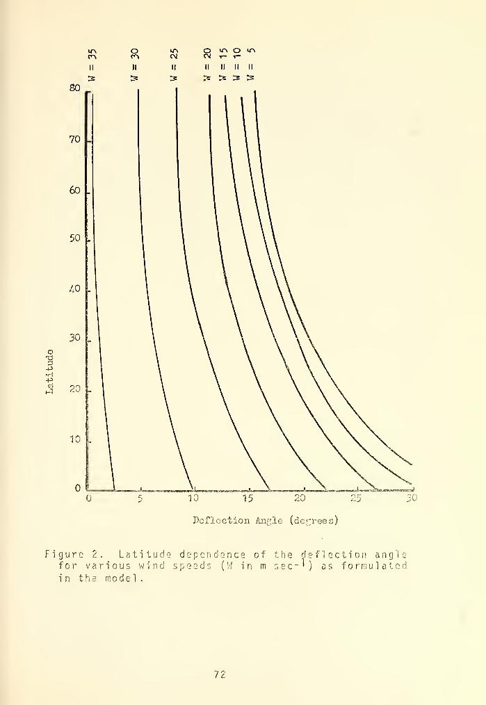
O O vr\ O1— T—
ir\
II II II II II II II
> 13 !3 5: > > S
oD-P•r!
-Pcrj
Deflection Angle (degrees)
Figure 2. Latitude dependence of the deflection anglefor various wind speeds (W in m sec-'') as formulatedin the model
.
72


ir» vrv
o
-p•H•PnJJ
10
CarstensenRollModel
15 20 25 30
Deflection Angle (degrees)
35
Figure 3. Latitude dependence of the deflection angleas found L»y Roll (broken line), Carstensen (solidline), and as formulated in the model for wind speeds( W ) of 5 m sec-1 and 15 m sec-1 (dashed lines).
73


oam
od)
O
10
-5
-10
-15
Residual
< J H
Figure 4 . Result of five point binomial filter appliedto a typical portion of a zonal component time seriesOriginal series (solid line) and filtered series(dashed line) arr> shown in the upper graph. Theresidual series is shown in the lower graph.
74

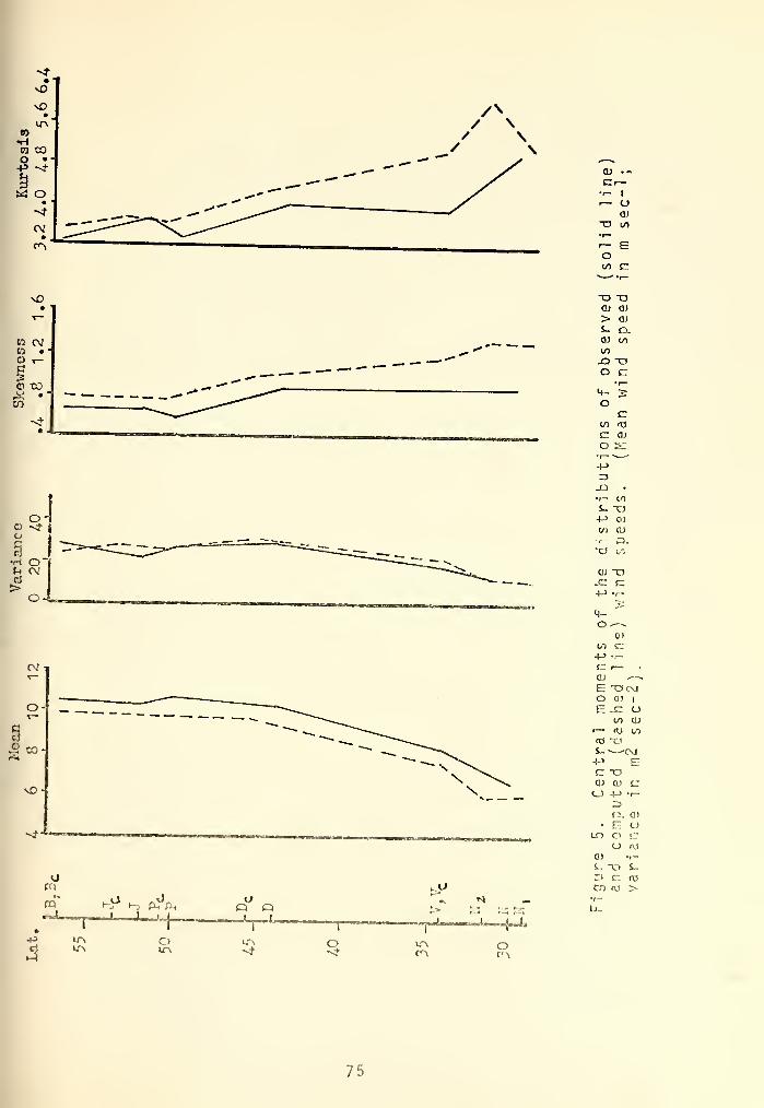
oo -^ro
ei
•HU
CV
sCO
sO-
uen
fQo
-*
+J,
irs
<u • •»
c r—
•
•r- 1
i
—
(J
<U
-a 00
•r—
1 Eooo c
•1
—
"O aaj a>
> a>
s_ D-0) oo
00
-Q aO c
•1
—
f- 2o
c:
oo fO
c: <D
o s:*(
—
^—
•
+J3-Q .
•i— in
S_ "13
+> 0)
1/1 (U
a.•a 0'*
<u "O-cr c+-> •.--
4-s
o ^^0)
00 rj+-> i—
iZ
a> ,—
>
E "OCMo ai i
E -C o00 QJ
r— ru 00
ra -os_-—-CSJ•(-' EC TJaj O) £J
o iJ -r-
3d. a>
• E oin O e
(J nj
0) r—s~ -o s-
n c: to
en ru >
oITS
O ITS O
75


-o 1
c uro OJ
CO
0J Ec
•1
—
c
TD +->
r— O)
O Cto O
>— O.Eo o
OJ O>S- i—a> <o
co c:
-O oO M
4- CO (O
a)
•I
—
jjr>
.Q to
•r— +->
+-> OJ
CO £3
•r- O
£a) oo
4- re
o co
co N
CM
c oO
I
-4-
I
N JV^___
_.
(tf
f -< *-r -s pSfal
3LT»Cf>
-"
OLA
a>«
LT\
-V
JL„
o
«.£ -
o
E -—^ •
OJ OJ'-^E CMO •.-
I
E r- OQ)
— to co
res a>i- -t-OJ+-> co Ea> ~o c:
"O 0)• a> u
cr> 4-> r:
aj cx-i-i- c j,
n o ra
CDU >
7G


CM
-4
to
•HtO sOo ••
W 00
o
toto
<D
o
i
00
or-
<D ot) ir\
§•H om r\>
cvl
o-
so
cv
sr
JS
o_J 4-L
O0^1
O
c-a <u
e c(O o
ex'— Eai oc o•r-
I— I
—
03
"D C•i- OI— »r-
o -al/) •!-
i-
O)
T=> Eai
> cs- *ai ai
vi s:-Q »
—
o
l/l
C (/)
O +->
•r- C+-> a>
rj c:
-Q or- CXS-- E+-> OCO O
•i
—
-a r— •
rOCVJ
oj c 1
x: o o4-> - ai
-a w4- -r-
O SwCXI
CJ Eoo E4-> c:
cr — •i—
O) OJ
E E <1>
O •<- oE r- c
ro
i— -a • r-
to a> $_
S- -£= (O+-> in >c fd
QJ -O .»
1 1 *—<>—
-a u• CD <u
(-. +5 in
^>
<u a. Es- E13 O cC7i O •r—
77


Ten Year Change In:
Lat.
Wind Speed-2 -1
Zonal Component-2-10 1
.55
-50
-U5
-40
.35
-30
\
Meridional Component-2-1 1 2
/
Figure 8 . Total change (integrated linear trend)over the ten year period from January 1960 throDecember 1969 in the observed (solid line) andcomputed (dashed line) wind speed and zonal andmeridional components (in m see-!)-
78


om
P
to
H
«oII
X!
(j_ 003 w) Qgajg a;ii;i CEIVTaOTVO = X
0)-(->
Q.Eoo
TDcro
aQJ
>S-
CD
10
-OO
CL>
-(->
c
a; cu
XI --3
(/> EC OO •<-
•i- +->
+-> ra
« +->
l— COa»i- c
c= a)
o o•r- OCO
<u o5- 4-
0) to
d; -aai
CD• D.
CXI 10
•o
•h|v,
79


S-
O4-
ir>c^
Ol
OJ
Q.to
IDO Cf\ i
—
ocu
<—* 4->T~
lf\ 13
CV CLo Eo om u6 c
11—OJo « 24->
cv 'A
PhCO _Ci
10
H C[3 o
o
a .;_}
> ("Ci
~-J i
—
tq OJ •
oo t- S-m OJo c -Q
iio B•r— OJ
|x! CO >L0 oOJ ^t:
S-
O) £=CI occ •r—
+->
re
o tor
--
c0) re
s~ OJ
n oCT>0
( L_ oss u
) aa&is c.'ii/i aaivmoivo - x
fiO


T3Ofi)
P.CO
noa•Ht2
'OQ)
-Pti
O
o
24-
18-
12_
6_
0_
1 2
1
132
1 2
;t 2i^4
22211
1 1211 111 13312923
1 313634211777V67 Hb721429A+3 4 * 4 J a 8
St>32LG8+ /G^t- U9'/» IbJUD> •*• D * i } H P/
EKLt>/P9PAKa'MLK
E/PusLa/iKfcMfcyMCN+I
J7
GBK9UE3n l :; b I b 4
G b > / + y 4
A A 3 b + A 4
bdlF4/ b 9 1 b 4
1
B293833324^3 2
53121 2
212 12121 32
3 1.
TD 12
r18 2^.
Observed Wind Speed (n aoc -1)
Figure 11. Scatter of observed and computed windspeeds (in n s e c - 1 ) at Ocean Station Juliet.Tabic IX defines the symbols.
81


oQ>Da
8oa.CO
c•H
O
ao
24-
.... ->."-'
Observed Wind Speed (m sec "')
Figure 12. Scatter of observed and computed windspeeds (in m sec"^) at Ocean Station Hovember.Table IX defines the symbols.
82


1.2 _
SpeedError
0.8
c 3 0.4
",
N-,
O
j5
1.6
1.2
0.8
0.4
-0.4
*
•vico^---?M$Q
*,
7>f,HHH
cio
sU'A
o o
1.2 „
0.8
0.4 .
o
V
100
?
fit
ft.
120 1^0 160 180
Separation Distance ( km )
200
Figure 13. Mean error (in m sec" ) dependence on
separation distance for wind speed arid the zonaland meridional components. Estimated best-fitlines are shown for components.
83


1.0
0.9
*S 0*8<DD,CO
a °- 7
0.6.
0.5
B
I
1.0-
«0.9
-f->
£jO
0.8O,
c
0.7rHc3
c *-v •0,6M
0.5
N,
&
-PC©
soo
o
o
1.0
0.9.
0.8 .
0.7 «
0.6
0.5
100
—gtJr-.fi -j »r— if i n iiiii flv»f
120 U0 160 180
Separation Distance ( km }
I
200
Figure 14. Linear correlation coefficient (R)dependence on separation distance for wind speedand the zonal and meridional components.
84


co•HjjidHo
oo-p
1.0J
0.8.
0.6
0.4
0.2 J
¥ 'U\K
0.0 . kc::
-0.2:.
w
Jsh,
.
KK
02'2
v 'V Cr At
*$
Log Time (hundreds of days)
Figure 15. Autocorrelation of observed (CO) endcomputed (XX) wind speeds at Ocean Station bravo
85


o•H
aO
5hOOO-P
1.0 .
0.8
0.6 .
0.4- .
0.2 .
0.0 .
-0.2
n.
^
002
Ml
A
1
to- • , r.
Lag Time (hundreds of days)
Figure 16. Autocorrelation of observe-*! (CO) andcomputed (XX) wind speeds at Ocean Station Victor
86


o•H-PaHo
ooo
1.0 -
0.3
0.6 -
0.4 -
0.2
0.0 .
-0.2:.
v./ n V 'fy
Lag Time (hundreds of days)
Figure 17. Autocorrelation of observed (CO) andcomputed (XX) zonal components at Ocean StationBravo .
87


1.0-
o•H-PCJHCD
^OOo+3
0.8.
0.6.
0.4--
o.;
0.0.
-0.2-
C\ w
Ki
,4
j:
Lag Tine (hundreds of days)
Figure 18. Autocorrelation of observed (CO) andcomputed (XX) zonal components at Ocean StationVictor.
88


o-pCJHo
hot>
o-p
1.0 _,
0.8
0,6
0.4-
0.2„
0.0
-0.2
'A-
Lag Time (hundreds of days)
Figure 19. Autocorrelation of observed (CO) andcomputed (XX) meridional components at OceanStation Bravo.
89


1.0
o.s
0.6 .
•H 0.4
rHOfH
Ooo-p
5s 0.2
0.0 .,
-0.2
F<
Log T.ir.e (hundreds of days)
Figure 20. Autocorrelation of observed (CO) andcomputed (XX) meridional components at OceanStation Victor.
90


cr r
LD
CD
>(XLlI
cr.
cch-uIjj
Ul
L'J
CC)
*A ,1
' if vy\iimw u
H\ i
mi
fV
\l^V I.
ill
0. JJ. 'f.llll o.sdu
Mi --<
LJ
d:LlJ
Xo*v**<r«wfrM#jm
a.soc ITT'* fl.Jfla (J. WJ
Frequency (cycles / day)
cr.
iCl.
as o.:oc 3.232 /jus s.«j ^ * j.::.:
? - 2Figure 21. Log energy density (in in sec" ), coherence, and
phase difference (in degrees) for computed and observedwind speeds at Ocean Station Bravo.
91


.r>
UJ «?
C~i
>LiCL
Li_l -I
UJ »,
SD
iVJ
"Y^
ii
(
:.2j
,f.wy«ij
C . j 00 nQJ~lCbOo
Frequency (cycles / day)
r
2 9Mgur-: 22. Log energy densi ty in (m sec ) , coherence, and
phase difference (in degrees) for computed 'and observedwind speeds at Ocean Station Victor.
92


^3-
O
to
mL • iUU
I
C3Q0 0-400 0-503
• . !
o
^ ^"^r^n^vn^/1Ay^v/Vi^y
i 1 i 1 ~iJ- i.0u
r 7P 0-500
Frequency (cycles / day)
o^V^V^A£lv^ ^\..aa,^fv^jw^a ,nv\A^ t-A ,\ /a
. . C-2C 0. 330 L • TO J
1n • o
2 - 2Figur-.? 23. Log energy densi ty (in m sec" ), coherence, and
phase difference (in degrees) for computed and observed7.o-,;.] components at Ocean Station Bravo.
93

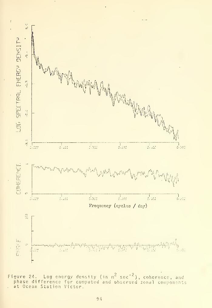
in
L.J
>
uJ
q:
%!'^1%
#Hiir
i
LiJX V
>::.
Frequency (cycles / day)
en
D.
r-« -V-i^tA/^^^/V^,
|
^ ,,'-,
V|-m j ",, ^ r**H\?%
7 ?Figure 24. Log energy density (in m sec ), coherence, andphase difference for computed and observed zonal componentsat Ocean Station Victor.
'.


>I—I—
I
LOz: •".
!_U <?a>CCSjJ
ZI mLU 4
dCC^—
01 ^,
0.300 U- 4l,w 0.500
z:
CCLUXDU o
'^^Y^^^
I
0.100-1 7 -. -.
300 0.500
Frequency (cycles / day)
LOen
000 '".':;. 0.200 0.J00 0-400 0.O.'IOO
2 - 2Figure 25. Lon energy density (in m sec ), coherence,
and phase difference for computed and observed meridionalcomponents at Ocean Station Bravo.
9 5


D~
in
uj <?
>(X
CC
LU ..
o. :n: 3. 2il£
"7~
UJITT
US
17.V"A\^^
Frequency (cycles / day)
2 - ?Figure 26. Log energy density in m sec ), coherence and
phase differences for computed and observed meridionalcomponents at Ocean Station Victor.
96


LIST OF REFERENCES
2.
7
8,
9
10,
11 ,
12,
Bakun, A., 1973: Coastal Upwelling Indices, West Coastof North America 1946-71 . NOAA Technical Report, NMFSSSRF-671 .
Bendat, J. S. and A. G. Piersol, 1971: Random Data:Analysis and Measurement Procedures . Wi
1
ey-Intersci ence ,
407 pp.
Bjerknes, J., 1969: Atmospheric Teleconnections fromthe Equatorial Pacific. Mon . Wea . Rev . , 97, No. 3,
p. 16 3-172.
Brummer, B., E. Augstein, and H. Riehl, 1974: On theLow Level Wind Structure in the Atlantic Trade. Quar .
Jour. Roy. Met. Soc. , 100, No. 423, p. 109-121.
Carstensen, L. P., 1967: Some Effects of Sea-AirTemperature Difference, Latitude and Other Factors onSurface Wind-Geostrophic Wind Ratio and Deflection Angle .
Fleet Numerical Weather Central Technical Note 29,Fleet Numerical Weather Central, Monterey, California.
Fleet Numerical Weather Central; 1974: The FNWC ComputerUser Guide, Edition 2 .
Monterey, California.
Freund , J . E
.
Hall , 390 pp.
Fleet Numerical Weather Central,
1962: Mathematical Statistics. Prentice-
Hal t i n e r , G. J. and F. L. Martin, 1957: Dynamical andPhysical Meteorology , McGraw Hill Co., 470 pp.
Hasse, L., 1974: On the Surface to Geostrophic WindRelationship at Sea and the Stability Dependence on theResistance Lav/. Beit. Phys . Atmos . , p. 45-55.
Mai k us, J. S., 1962 : Large Scale Interactions. In Th e Se a
Vol. I, M.N. Hill Ed., I ntersci en ce , p. 88-294.
Munk, W. H.
Met . , 17, p
1960: Smoothing and Persistence92-93.
Jour
Namia"s, J., 1963: Large Scale Interaction Over theNorth Pacific from Summer 1962 Through the SubsequentWinter. Jour. Geophys. Resch ., Vol. 68, No. 22,pp. 6171-6186.
97


13. Panofsky, H. A. and G. W. Brier, 1968: Some Applicationsof Statistics to Meteorology . Pennsylvania StateUni versi ty , 224 pp
.
14. Roden, G. I., 1974: Thermohal i ne Structure, Fronts, andSea-Air Energy Exchange of the Trade Wind Region Eastof Hawaii. Jour. Phys. Ocean . 4, No. 2, p. 168-182.
15. Roll, H. U., 1965: Physics of the Marine Atmosphere .
Academic Press, 426 pp.
16. Seckel , G. R., 1970: The Trade Wind Zone OceanographyPilot Study Part IV: The Sea Level Wind Field and WindStress Values July 1963 to June 1965 . Bureau ofCommercial Fisheries Special Scientific Report, FisheriesNo. 620.
17. Spiegel, M. R., 1961: Statistics , Schaum's OutlineSeries. McGraw-Hill 395 pp.
18. Taylor, A., 1955: Advanced Calculus . Blaisdell, 768 pp.
19. Tennekes, H. and J. L. Lummely, 1972: A First Course inTurbul ence . The MIT Press, 300 pp.
20. Verploegh, G., 1967: Obser vatio n and Analysis of th e
Surface Wind Over the Ocean . Koninklijk Neder landsMeteorologiscn Institutt, Mededelinger En Verhandelinqen,No. 89, 68 pp.
21. White, W. B., and A. E. Walker, 1973: MeridionalAtmospheric Teleconnections Over the North Pacific.Mon. Wea. Rev ., 101, No. 11, p. 817-822.
9 8


INITIAL DISTRIBUTION LIST
Defense DocumentationCameron StationAlexandria, VA 22314
Center
No. Copies
2
Library, Code 0212Naval Postgraduate SchoolMonterey, CA 93940
Department of Oceanography, Code 5!
Naval Postgraduate SchoolMonterey, CA 93940
Professor G. Jung, Code 58JgDepartment of OceanographyNaval Postgraduate SchoolMonterey, CA 93940
Professor R. Elsberry, Code 51 EsDepartment of MeteorologyNaval Postgraduate SchoolMonterey, CA 93940
Oceanographer of the NavyHoffman Building No. 2
200 Stovall St.Alexandria, VA 22332
Office ofCode 480Arlington,
Naval Research
VA 22217
Dr. Robert E. StevensonScientific Liaison Office, 0NRScripps Institution of OceanographyLa Joll a, CA 920 3 7
Library, Code 3330Naval Oceanographic OfficeWashington, DC 20373
10. SI0 LibraryUniversity ofP.O. Box 2367La Jol la , CA
California, San Diego
92037
9 9


11.
12.
13
14
15
16.
Department of Oceanography LibraryUniversity of WashingtonSeattle, WA 98105
Department of Oceanography LibraryOregon State UniversityCorvallis, Oregon 97331
Commanding OfficerFleet Numerical Weather CentralMonterey, CA 93940
Commanding OfficerEnvironmental Prediction Research FacilityNaval Postgraduate SchoolMonterey, CA 93940
Department of the NavyCommander Oceanographi c System PacificBox 1390FPO San Francisco 96610
No. Copies
1
1
Mr. Sigurd LarsonEnvironmental PredictionNaval Postgraduate SchoolMonterey, CA 93940
Research Faci 1 i ty
100


29 JAN £02 6 U 06
* 57210Larson
,A statistical
f '«tio„ of a '6ri -
29 «M«eo• 26UQC
Thesi i
L2743 Larson
c.l A statistical veri-fication of a ten >", a'-
series of computed
surface wind conditions
over the North Pacificand North Atlantic
Oceans
.
157210

thesL2743
A statistical verification of a ten year
HIM
3 2768 002 12264DUDLEY KNOX LIBRARY