A STATISTICAL EVALUATION OF MINERAL DEPOSIT SAMPLING

by

HOWARD W. BRISCOES. B. , Massachusetts Institute of Technology

(1952)

SUBMITTED IN PARTIAL FULFILLMENT OF THE

REQUIREMENTS FOR THE DEGREE OF

MASTER OF SCIENCE

at the

MASSACHUSETTS INSTITUTE OF TECHNOLOGY

June 1954

Signature of Author ______Department of Geology and Geophysics May Z4, 1954

Certified byThesis Supervisor

Accepted byChairman, Departmental Committee on Graduate Students

ACKNOW LEDGMEN TS

The author wishes to express his appreciation to Professor

Roland D. Parks, for supervising this thesis. Acknowledg-

ment is also made to Dr. L. H. Ahrens, and Enders A.

Robinson for their kind cooperation and suggestions.

A STATISTICAL EVALUATION OF MINERAL DEPOSIT SAMPLING

by

Howard W. Briscoe

Submitted to the Department of Geology and Geophysics onMay 24, 1954 in partial fulfillment of the requirements for thedegree of Master of Science.

Abstract

If the procedure of mathematical statistics are to be used to improvethe analysis of a set of samples of any kind, the samples being analysedmust be statistically unbiased; and some information about the size or dis-tribution of the population being sampled must be available. The geologicmeaning of a statistically unbiased sample is discussed with respect to col-lecting and weighting the sample units. An investigation of the presentlyavailable knowledge about the distribution of geologic populations indicatedthat the expected log-normal distribution does not hold for all kinds of de-posits, and there are indications that the shift from the log-normal distri-bution may be related to the effect of weathering of the deposit. A morethorough study is needed before any safe conclusions about the generaldistribution of elements in various geologic bodies can be reached.

Possible statistical aides in detecting zoning in geologic deposits arediscussed. These procedures are based on the number or length of runsof values above and below the mean or median of an ordered sequence ofsamples.

The use of the " t distribution for estimating the average assay valueof a deposit from the assay values of samples taken from the deposit is de-scribed, and possible variations on the procedure are discussed.

Finally, the method of Sequential Analysis and its potential geologicapplications are considered. The use of Sequential Analysis based on thedistribution of the sampled population is impractical without a more de-pendable knowledge of the analytic form of this distribution, but the use ofSequential Analysis based on the distribution of the mean of all possiblesamples of a fixed size merits further investigation.

TABLE OF CONTENENTS

I. INTRODUCTION 1

II. THE STATISTICAL NOTION OF A SAMPLE 2

The Sample Universe and Unit Samples. 2

Geologic Sampling. 4

III. NONHOMOGENEOUS DEPOSITS 5

Sample Patterns and Weighting Factors. 5

Detection of Zoning 7

Error Resulting from the Methods of Cutting Samples 11

IV. THE SELECTION OF A TEST FOR ESTIMATING THE 13

AVERAGE VALUE OF A DEPOSIT

Errors and Confidence Limits. 13

Frequency Distribution of Geologic Samples. i5

Tests Based More Widely Applicable Assumptions. 18

V. A VALID STATISTICAL PROCEDURE FOR ESTIMATING THE 20

AVERAGE ASSAY VALUE OF A GEOLOGIC DEPOSIT

The Basis for the Analysis. 20

The Procedure for Estimating the Assay Value of the 2z

Deposit.

An Example of the Use of the " t 8 Distribution. 22

An Evaluation of the Procedure and its Variations. 23

VI. SEQUENTIAL ANALYSIS 27

The Application of Sequential Analysis Based on the 28

Distribution of the Sample Universe.

Application of Sequential Analysis Based on the a t 29

Distribution.

VII. SUMMARY

TABLE OF CONTENTS (continued

TABLES I and II 31

TABLE III 32

FIGURES 34

APPENDIX A i

TABLE IV ii

REFERENCES iv

BIBLIOGRAPHY v

I. INTRODUC TION

Thousands of dollars each year are spent for sampling geologic bodies,

and millions of dollars are spent each year on the basis of the results of

these samples. As a result, the problems of effectively sampling mineral

deposits and of reliably interpreting the resulting samples have been con-

sidered imaginatively; intuitively; empirically; and even, occasionally,

mathematically.

The application of imaginative, intuitive, and empirical methods is

limited only by the fact that the accuracy of the results is somewhat unpre-

dictable. On the other hand the mathematical approaches offer controlled

accuracy but are limited by, first, the validity of the assumptions on which

the mathematical method is based; second, the geologist's ability to under-

stand and correctly use the mathematics involved; and, third, the extent

of the calculations that must be made to use the test.

In this paper, the application of several statistical procedures to the

design of efficient methods of sampling of geologic bodies will be investi-

gated. Specifically, the statistical interpretation of samples and its effect

on the procedures for cutting samples will be considered first. Next the

use of statistical tests of randomness of a series of numbers will be con-

sidered as a method of testing for zoning in a deposit, and a method of

obtaining statistical confidence limits on the average assay value of a

geologic body from a series of samples will be described. Finally the

possible value of applications of the techniques of sequential analysis to

geologic sampling will be discussed.

It must be realized from the start that statistics, at best, can be used

only as a valuable tool to help the geologist to answer, on a mathematical

basis, a few of the many problems that confront him. The problem is still

a geologic problem, and the parts of the problem to be analysed statistically

must be clearly defined and must supply some information about the geology

of the deposit. It would be a waste of time, for example, to spend several

hours testing a deposit for possible zoning if the geology of the deposit was

such that it was sure to be zoned. The statistical tests alone can have no

value. The assumptions which form the basis for the tests must be

geologically reasonable, and the results of the test must be such that they

can be interpreted geologically.

II. THE STATISTICAL NOTION OF A SAMPLE

Geologic samples may serve several purposes; they may be used to

help determine the geologic structure or age of a deposit; they may be

used to investigate the ease with which certain valuable ingredients can be

separated from the gangue or freed from the chemical compounds in which

they are found; they may be used to determine boundaries of commercial

deposits; or they may be used to estimate the grade of a deposit that is to

be mined. The concept of the sample is different for each of the purposes

for which a sample is to be used; however, the same sample may serve

more than one purpose. In one case the sample may be considered as a

collection of fossils or sand grains; in another the sample may be con-

sidered as an aggregate of chemical compounds. When the samples are

to be used to outline a deposit, each sample must be considered as repre-

senting a specific part of the deposit, most commonly the volume of the

deposit bounded by the surface equidistant from that sample and the sur-

rounding samples closest to it.

The most valuable applications of statistics are associated with sampling

to estimate the grade of a deposit, and the concepts and characteristics of

samples taken for this purpose will be considered in some detail.

The Sample Universe and Unit Samples.

In order to develop the concept of a geologic sample which is appropriate

for statistical purposes, the geologic body being sampled is divided into

a large number of small parts, each of equal size and similar shape. The

aggregate of all of these small parts will be referred to as the 'sample

universe," and each part will be called a "sample unit. " A "sample of

size N" will refer to any group of N individual sample units. For

simplicity, this discussion will assume that the assay value of each sample

unit can take one of a finite number of possible values (this assumption is

valid in that it is possible to measure the concentration of any component

of the sample unit to only a finite accuracy, say to . 01, percent of the weight

of the sample unit). If the assay value in percent of the weight of the sample

unit is plotted as the abscissa and the number of sample units in the sample

-2-

universe which have the given assay value is plotted as the ordinate, the

resulting curve is the "frequency distribution" of the sample universe. The

frequency distribution of the sample universe completely describes the

amount of the interesting component in the deposit and the variation of the

concentration of that component, but that it does not describe the geometry

of the zoning in the deposit is obvious since no measure of distance or

direction is involved. The average assay value of the universe of samples

is the value of the abscissa such that equal areas lie under the parts of the

curve on each side of it.

If the assay value is plotted as the abscissa, and for every assay value

the percent of the number of samples in the sample universe with that assay

value or less is plotted as the ordinate, the resulting curve is the *cumu-

lative distribution' or simply "the distribution" of the sample universe.

The average assay value is that value of the abscissa corresponding to an

ordinate of 50 percent. Any two samples for which the ratios of corres-

ponding ordinates of the frequency distributions are equal will have the same

cumulative distribution.

The statistical concept of a sample is based on the fact that a random

sample of size N will tend to have a distribution similar to the distribution

of the universe being sampled. As N is increased, the distribution of the

sample is increasingly likely to be similar to the distribution of the uni-

verse; and, when N includes all possible sample units, the distribution of

the sample must be the same as the distribution of the universe.

The various procedures for statistical sample analysis are based on

determining the probability that the sample taken has a distribution similar

to the distribution of the universe. In general the sample alone is not enough

information on which to base a rigid test. At least the size of the sample

universe must be known before any calculations can be made to determine

the probability that the sample distribution will be similar to the distribution

of the universe. Usually some information about the actual distribution of

the universe or of some characteristic of the sample is known, and all

statistical tests that have been developed place some requirement on the

minimum amount of information that must be used in that test. The infor-

mation used by many tests is in the form of one or more assumptions

-3-

concerning the distribution of the sample universe and may not ever enter

the analytic formulas for applying the test, and it is important that the

validity of the assumptions be considered before the test is applied. It is

evident that a statistical test which uses as much of the available infor-

mation as possible should be chosen for any analysis because the more

information the test has to work with the more reliable the results of the

test will be for a given sample.size.

Geologic Sampling.

If geologic samples are to be considered statistically they must be un-

biased; that is, they must be representative of a universe of sample units.

The most obvious way of getting biased samples would be to take most of

the samples from a zone that is not representative of the whole deposit, a

zone of high grade ore for example. The use of improper weighting factors

in computing the average assay value of the sample will also result in a

biased sample because such weighting factors would cause certain samples

to receive undue emphasis. A third cause of biased samples may be con-

centration or dilution of the samples while they are being cut.

Another form of error can be introduced into the samples by taking

sample units of different sizes. Consider, for example, a deposit in which

the interesting component of the rock occurs in the form of masses of one

pound or less. If the size of the sample unit is one pound, it is possible to

get an assay value of 100 percent; but, if the size of the sample unit is five

pounds, the maximum possible assay value is 20 percent. Thus a sample

composed of both sizes will result in an inconsistent sample frequency dis-

tribution and a biased sample.

The closer the sample universe comes to being a homogeneous mixture

of the valuable constituent and the gangue, the smaller the error introduced

by any of the errors listed above will be. In extremely erratic deposits,

like many gold deposits, it may be very difficult to get a safely unbiased

sample.

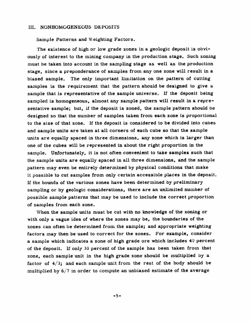
III. NONHOMOGENEOUS DEPOSITS

Sample Patterns and "\eighting Factors.

The existence of high or low grade zones in a geologic deposit is obvi-

ously of interest to the mining company in the production stage. Such zoning

must be taken into account in the sampling stage as well as the production

stage, since a preponderance of samples from any one zone will result in a

biased sample. The only important limitation on the pattern of cutting

samples is the requirement that the pattern should be designed to give a

sample that is representative of the sample universe. If the deposit being

sampled is homogeneous, almost any sample pattern will result in a repre-

sentative sample; but, if the deposit is zoned, the sample pattern should be

designed so that the number of samples taken from each zone is proportional

to the size of that zone. If the deposit is considered to be divided into cubes

and sample units are taken at all corners of each cube so that the sample

units are equally spaced in three dimensions, any zone which is larger than

one of the cubes will be represented in about the right proportion in the

sample. Unfortunately, it is not often convenient to take samples such that

the sample units are equally spaced in all three dimensions, and the sample

pattern may even be entirely determined by physical conditions that make

it possible to cut samples from only certain accessible places in the deposit.

If the bounds of the various zones have been determined by preliminary

sampling or by geologic considerations, there are an unlimited number of

possible sample patterns that may be used to include the correct proportion

of samples from each zone.

When the sample units must be cut with no knowledge of the zoning or

with only a vague idea of where the zones may be, the boundaries of the

zones can often be determined from the sample; and appropriate weighting

factors may then be used to correct for the zones. For example, consider

a sample which indicates a zone of high grade ore which includes 40 percent

of the deposit. If only 30 percent of the sample has been taken from that

zone, each sample unit in the high grade zone should be multiplied by a

factor of 4/3; and each sample unit from the rest of the body should be

multiplied by 6/7 in order to compute an unbiased estimate of the average

-5-

value of the deposit. Since the correction is a correction on the frequency

of the occurrence of the sample unit in the sample, the unbiased estimate

of the variance must be found from the formula

sZ = (xi )2 fw/N + I (1)

where f is the frequency of sample units with value xi , x is the unbiased

estimate of the mean, and w is the weighting factor (4/3 for samples in

the zone and 6/7 for those not in the zone in the example above). If the

nature of the zone is very difficult from the rest of the deposit, the use

of the corrective weighting factors may not result in truly unbiased

samples. When the zones are so different that the use of weighting factors

is invalid, it is likely that the zones will require different metallurgical

methods for refining the ore, or that different methods will be used to mine

the zones, and the separate zones will be treated as separate deposits.

The application of various weighting factors to geologic samples is a

common practice; however, many of the weighting factors are not based

on statistically sound reasoning and will actually cause the samples to be

biased. Weighting functions involving powers of the frequency or assay

values of the unit samples along a fixed direction are often used to correct

for geometric considerations in the deposit. These weighting factors, par-

ticularly factors of the square or cube of the frequency are valid for a few

special combinations of zoning geometry and sample pattern; but the

general use of weighting factors based on a fixed function of the frequency

is unsound and may result in serious errors. Any legitimate weighting

function that is used to correct for nonhomogeneity of the deposit must be

oased on some knowledge of the relative size and the relative grade of the

various zones and must be logically designed to cause each zone to be

represented in proportion with its size in the final estimates of the para-

meters (average assay value, variance, etc.) of the distribution of the

universe.

The units used for expressing the assay values may introduce an un-

sound weighting factor into the values of the sample units. Assay values

should be measured in units equivalent to the percent of the volume or

weight of the sample unit that is accounted for by the constituent being con-

sidered. Units of pounds-of-x per pound-of-sample or cubic-feet-of-x per

cubic -foot-of-sample (where x is the constituent of the sample that is of

interest), for example, would be appropriate units for the assay values.

When the assay values are found by multiplying the percent of x by half

the distance to the adjacent samples, the distance factor is actually a

weighting factor and may place undue emphasis on certain samples which,

for some reason unrelated to the assay value, have more than the average

spacing between samples. Hidden weighting factors of this kind are

probably the most common error in current geologic sample analysis

procedure.

Detection of Zoning.

The existence of zones in many deposits can be determined from geo-

logic information before any samples are taken, and the boundaries of

many zones coincide with geologic boundaries which are also known before

samplinghas been started. In other cases the zones may not be recognized

until preliminary or even final samples have been taken, but by the time the

sampling has been finished any zones existing in the deposit except those

that are smaller than the sample spacing should have been recognized or

at least suspected. If zones are completely missed by the sample pattern

or are arranged such that they appear as random variations in the sample

values, there is no way to detect their presence except closer sampling.

When zones are not expected or detected by the sampling, they will usually

not be large enough to have an important affect on the average assay value;

or, if they appear as random variations in the samples, the sampling

pattern may give a representative sample in spite of the zones. There will,

of course, be a few isolated cases where important zoning will go undetected

and the sample will be misleading, but these cases will be rare if a reason-

able number of sample units are taken throughout the deposit.

Exceptional cases in which reasonably large zones of slightly high or

low grade ore must be detected may occur occasionally, and in such cases

there may be some question about the significance of a group of sample

units that are consistently above or below the average assay value by a

-7-

small margin. In these rare cases statistical tests can be used on the

samples along any line through the suspected zone to find the probability

that the given sequence of values is a random sequence. Two such tests

will be considered here.

Consider an ordered sequence of numbers each of which must come

from one or the other of two mutually exclusive classes of numbers.

Any group of one or more consecutive numbers from the same class will

be referred to as a run. If the sequence contains r numbers from Class

I and s numbers from Class II and if the sequence is a random sequence,

all possible combinations of r numbers of Class I and s numbers of

Class II are equally probable; and the probability of getting k runs in the

sequence of T = r + s numbers is

(r-i) I(s-i)! r! s!P(k) z (2)(k/2-1)!(k/2-1)!(r-k/2)!(s-k/2). T !

if k is even, and

(r-l)!(s-l)! r! s! I 1P(k) k + k-1 (3)

kk+1 k- k k+ 1. "' . T. r r * 5--.'2 2 L 2 2 2 2

if k is odd.

A sequence of numbers filling all the requirements of sequence just

described can be constructed from the consecutive assay values of sample

units along a line through a suspected zone by computing the deviation of

each value from the mean assay value for the sample units along that line

and associating positive deviations with one class and negative deviationswith the other class. If the line along which the samples are taken passes

through a zone, all combinations of positive and negative deviations are

not equally probable; but all possible sequences are equally probable if

the line lies entirely within one homogeneous zone.

The probability of getting more than A runs and less than B runs in a

random sequence can be found from the probability, P(k), of k runs by

using the formula

-8-

k=B k=B k=AP(A < k < B) = P(k)= Z P(k)- Z P(k). (4)

k=A k=2 k=2

A test for the randomness of a sequence of numbers can now be made

by determining the minimum number, A, and the maximum number, B,

of runs such that the expected number of runs from a random sequence

will be between A and B in a predetermined percent of the possible se-

quences. The predetermined percent of the time that k will be between

A and B is known as the "level of significance, " and the values of A

and B that result in a given level of significance are the values of A and

B for which P(A < k < B) is equal to the significance level. The use of

such a test has been made practical by published tables of the probability

that k will be between 2 and B. The probability is tabulated as a function

of r, s, and B. 2 We may reject the hypothesis that the series is random

if there are either too many or too few runs in the series, and in any test

values of A and B should be determined so that the probability that k is

less than A is equal to the probability that k is greater than B. This

condition will be satisfied if

1 A=B kaP(k < A) = P(k > B) - P(k) + P(k)

k2 12 Z

(5)

An example may help to clarify the test described above. Consider the

sequence of average assay values from the line of drill holes listed in table

I. This sequence was taken from the test holes along the line 500 W in the

lateritic iron deposit described in Appendix A. For this sequence

r=-5

so-5

k=-7

and the values of A and B such that

P(A < k KB) = .95

will be determined. Thus the level of significance will be 95 percent.

From Eq. (5) the probability that k is less than A is found to be

I/'2 1 - P(A< k< B) or P(k< A) = 1/2 (1 - .95) = 1/2 (.05) = .025.

-9-

The probability that k is less than 13 is one minus the probability that k

is greater than B, so that

P(k < B) = I - .025 =.975.

The required values of A and B such that

k=B2 P(k) -=. 975

k=Z

and

k=BP(k) = .25

k=4

are looked up in the tables and are found to be

A=-2

B - 9,

and the sequence is found to be random since the value of k in the sequence

seven.

In some cases it may be more appropriate to base the test on the prob-

ability of getting a run as long as the longest run in the sequence rather than

the probability of getting the number of runs found in the sequence. A test

based on the probability of getting a run of size s on either side of the

median of a sequence and the tables for using the test have been derived.

The computations involved in setting up the tables for this test are more

complex than those for the test based on the number of runs, and the for-

mulas will not be reproduced here. On the other hand, the use of the tables

is simpler because, first, the hypothesis of a random sequence can be re-

jected only on the basis of a run that is too long and, therefore, only one

value must be looked up in the table; and, second, the test is based on

runs above and below the median instead of the mean so the probabilities

need be tabulated only for two variables, the number of samples in the se-

quence and the size of the run. The tables available for this test are rather

limited.

-10-

The length of run for which the hypothesis of a random sequence should be

rejected on the 95 percent significance level is tabulated as a function of

the number of samples in the sequence in table II.

Applying this test to the sequence described in table I to determine

whether the sequence is random on a 95 percent significance level it is

found that the number of samples is ten and the longest run is a run of

two which is shorter than the run of five needed to reject the hypothesis

of a random sequence, and the sequence is found to be a random sequence.

In each of these tests the acceptance of the hypothesis of a random se-

quence is associated with a lack of significant zoning along the line of

samples being tested.

Clearly, any test for zoning which is based on the number or size of the

runs of high and low values can detect only those zones which are large

enough or have sufficient contrast to affect the size or number of the runs

and will not detect many possible configurations of small zones. The test

oased on the number of runs will be more effective for detecting small

zones with high contrast between zones because the high contrasts will

place the mean safely between the two zones so that each zone will be one

run and the number of runs will be small (approximately equal to the

number of zones along the sequence).

Errors Resulting from the Methods of Cutting Samples.

Dilution or concentration of samples as a result of the method used to

cut samples has been mentioned as a possible cause of biased sampling.

Obviously cutting procedures that may introduce errors into the samples

should be avoided; but, often, there is no other way to get the samples;

and in these cases the assay values of the samples are usually adjusted to

correct for the error. Here, again, zoning in the deposit may complicate

the problem since a zone of nigher or lower grade ore than the rest of the

deposit is often also a zone of different physical characteristics (more

friable or more coarsely crysialline for example) from the rest of the

deposit. Thus, the error resulting from cutting the samples may differ

in the various zones because the ability to cut a good sample depends on

the tendency of the rock to crumble. As a result, weighting factors in

zoned deposits may have to be designed to correct for cutting errors as

well as the proportion of samples in the various zones. The determination

of such weighting factors must be based on experience with the procedure

being used to take samples.

Weathered zones, contact zones, and other zones that are not typical

of the main body of the deposit must be considered in a similar manner to

zones while taking samples. The method used to cut the sample units and

the sampling pattern must be such that a preponderance of samples is not

cut from unimportant zones of this kind.

IV. THE SELECTION OF A TEST FOR ESTIMATING THE AVELAGE

VALUE OF A DEPOSIT

Once the size and shape of the geologic deposit have been found and

weighting factors to account for zoning, cutting errors, and other possiole

errors have been determined, the problem becomes one of estimating the

grade of the deposit; and this is primarily a statistical problem. Several

tests are available for the estimation of the average assay value, and a

number of factors must be considered before choosing the test to be used.

Errors and Confidence Limits.

The purpose of sampling for the grade of a deposit is primarily to de-

termine whether the concentrations of the various significant constituents

are within the limits which define a commercially valuable deposit. The

analysis may result in information in one of several forms all of which

satisfy the basic purpose of the sampling; but some forms supply more

additional information than others. The most common tests result in

either rejection or acceptance of a hypothesis that the mean of the sample

universe has a given probability of lying within certain predetermined

limits, or they determine the confidence limits above and below the mean

of the sample within which the mean of the universe will fall with a pre-

determined probability. The latter result is usually preferable because

it gives the limits within which the mean of the universe is expected to be,

regardless of how high or low the limits are, instead of merely determining

whether the mean is expected to be in a fixed interval.

The final decision made on the basis of the statistical analysis of the

sample may make one of two possible errors. An "error of the first kind"

is made when the average assay value of the sample universe is actually

within the limits of a commercial deposit and the results of the analysis

indicate that the average assay value is not within these limits. An "error

of the second kind" is made when the average value of the universe is not

within the commercial limits and the analysis indicates that it is within

these limits. A decision to accept the hypothesis that the average assay

value is within the commercial range is seldom questioned. As soon as

-I3-

the decision is made, mining operations are begun; and large sums of

money may be put into the mining of a deposit before an error of the second

kind is detected. On the other hand, when the analysis of the sample indi-

cates that the deposit is not a commercial deposit, the deposit will probably

either be subjected to more detailed sampling, or it may be set aside until

the commercial limits change, but it will not often be completely discarded.

Thus either kind of error may be costly and, ooviously, undesirable; but an

error of the second kind may be more costly than an error of the first kind

unless the mining company doing the sampling depends on the success of the

deposit in question for its existence.

The ideal test, then, is one which allows the probability of an error of

either kind to be determined or, preferably, preset. There are, however,

very few tests that allow both errors to be controlled. Even the choice of

which error is to be controlled is not usually open to the investigator; al-

though there are usually some practical reasons for preferring control

over a particular error. The test chosen should, of course, be the one

which leads to the smallest error of one kind when the error of the other

kind is fixed. However, it is often extremely difficult or even impossible

to determine the error not involved explicitly in the test.

If the error of the first kind is to be reduced to zero, we must accept

the hypothesis that the deposit is of commercial value all of the time. This

would make the probability of an error of the second kind rather high. Con-

versely, reducing the probability of an error of the second kind to zero re-

quires that the hypothesis should never be accepted, and the probability of

an error of the first kind is, then, large. Thus, the extreme reduction of

one error will cause an increase in the other, and the practical use of a

statistical test requires that a compromise which does not ask too much

safety in either direction be found.

The statistical probability of error, significance level, or percent of

confidence interval should not be confused with the tolerance limit on the

assay value. For example, if the 95 percent confidence interval on the

mean of a distribution is 100 + 10, it means that in 95 percent of the

possible occurrences of the sample taken the sample will be from a uni-

verse with an average value between 90 and 110. The tolerance limits on

-14-

the mean are 10 percent above or below the estimated mean of 100 for this

case, but the level of significance of the statistical test is 95 percent. The

significance level and allowable tolerance limits are not independent, and

for a given sample size an attempt to get an extremely high significance

level will result in wide tolerance limits. For geologic sampling a sig-

nificance level greater than 95 percent may be unwise and even unrealistic

in that it may be expecting an absolute guarantee from a statistical method.

In the various stages of the sampling procedure, from the preliminary

survey to the final production control, tolerance limits of from 10 percent

to less than one percent are not unreasonable.

Frequency Distribution of Geologic Samples.

It has already been pointed out that some information besides the sample

itself is needed for the statistical analysis of the sample, and a test which

uses as much information as possible should be chosen for any analysis.

The procedure should not use any information that is subject to any doubt,

however. The most desirable situation is one in which the available infor-

mation is in the form of an assumption concerning the frequency distribution

of the universe from which the sample was taken. The maximum amount of

information in this form would be a knowledge of an analytical expression

for the frequency distribution of the universe in which the parameter being

estimated (the average assay value in geologic work) appears as the only

unknown parameter. Almost all of the statistical procedures that have

been worked out in detail are based on the assumption that the universe has

one of three convenient analytical forms in which the distribution is com-

pletely described by three parameters or less. These three distributions

are the normal, the Poisson, and the binomial distributions. The binomial

distribution is concerned with the distribution of sample units which may

take either of two specific values when the probability of a sample unit of

each value is known, and it is not a distribution that could apply to geologic

samples. The Poisson distribution occurs as the limit of several forms of

distributions as the samples get large subject to certain restrictions and

would not be expected as the distribution of a geologic sample. The normal

distribution is the only one of the three common distributions that may fit

-15-

the distribution in a geologic deposit, and it is a distribution that occurs

quite commonly in nature.

Before attempting to choose an efficient statistical procedure for ana-

lysing geologic samples, it is imperative that the expected nature of the

distribution of the universes from which the samples will be taken should

be investigated. If the distribution is found to be normal, a wealth of

procedures allowing either or both of the two kinds of errors to be deter-

mined will be available for estimating the mean of the assay value of a

deposit. There is reason to believe that geologic distributions will not be

normal, but that they will be log-normal. 4 This means that the distribu-

tion of the log of the assay values of the sample units will be normally

distributed, and that an analytic expression for the distribution is available.

To determine the distribution of the assay value of the sample units in

a geologic deposit, the deposit would have to be completely mined out in

units the size of the sample units that would be used for sampling. Each

unit would have to be analysed separately because any combining of the

samples before the chemical analysis would smooth the distribution. Such

a procedure is obviously impossible, and some other method must be used

to determine the desired distributions. If the distribution is to be of any

practical value, it must hold for all deposits, or for a very large class of

them. A distribution that is sufficiently universal to be useful should be

evident in the samples from a large number of deposits.

The investigation of the distributions of elements in geologic deposits

was based on 17 sample distributions from seven mining properties sampled

by the United States Bureau of Mines, 5 an article on drill core sampling in

the Whitwatersrand, 6 and the iron deposit described in Appendix A. Ofthese deposits one is in the soft, altered material in a volcanic agglomerate;

three are laterites; one is a contact metamorphic deposit; one is a re-

placement deposit in sedimentary strata; two are sedimentary; and one is

in a schist. The distributions found in these samples can be divided into

two groups. The log-normal distribution found in igneous rocks by Dr.

Ahrens4 also appeared in all the samples of the contact metamorphicdeposit, in all the sedimentary deposits, in the replacement deposit, in the

schist deposit, and in the non-metallic constituents (SiO 2 , sulphur, and

-i6-

phosphorous) of a laterite deposit (see figures I and Z). The characteristics

of the second group were not clearly determined, but the distributions tended

to be more symmetric than the log-normal distribution and varied from Dti-

modal to slightly negatively skewed distributions (see figures 6, 7, and 8).

The samples whose distribution fell into the second group included the metal-

lic constituents (iron, nickel, and chromium) of the laterites and the deposit

in the altered volcanic agglomerate.

The results of this investigation have suggested several interesting

directions in which further work may prove valuable. Most of the samples

used were taken as part of preliminary investigations of geologic bodies and

were not designed to accurately determine the details of the distribution of

the deposits; and, therefore, the following discussion must be treated as

mere speculation until considerably more work is done to prove or disprove

the suggested theories.

Figures I and 2 are frequency distributions for two of the deposits with

typical log-normal distributions. The cumulative distributions of the logs

of these values are plotted on normal probability paper in figures 3 and 4.

If the distributions are log-normal, the plots in figures 3 and 4 should be

straight lines. The curve in both these lines indicates a tendency to have

too many values greater than the peak value, and neither distribution is

actually log-normal. One of the deposits that has a log-normal distribution

(a barite deposit that replaces sedimentary beds) has been sampled by trench

and drill samples, and the frequency distributions of the two kinds of samples

are plotted in figure 5. The trench samples are found to have a higher per-

centage of samples after the peak than the hole samples. If the trenches

were in a weathered zone along the surface of the deposit, the shift in the

frequency distribution may be related to the weathering. it is not statisti-

cally sound to make such a general statement on the basis of one example,

and a much more thorough study should be made before the suggestion can

be seriously considered. If the second kind of distribution can be considered

as the end result of the shift in the frequency distribution, however, the fact

that this distribution seems to occur only as the result of extreme weather-

ing would support the suggestion that the shift is due to weathering. The

degree of shifting of the frequency distribution of a sample from the log-

-17-

normal distribution may even provide a quantitative measure of the degree

of weathering in the zone from which the sample was taken.

Once the characteristics of the frequency distributions for various kinds

of deposits have been determined they may be used as a check for sample

errors. If the distribution of a sample is not similar to the characteristic

distribution for the type of deposit it was taken from, there may be reason

to believe that the sample is not representative of the deposit; that errors

have been introduced by the cutting method; or that the geologic interpre-

tation of the deposit has not considered some important factor such as

weathering. The second possibility may be most important practically,

for it has been shown that some methods of cutting samples may introduce

large errors into the samples. 6 In the case of the carbon lead of the

Whitwatersrand the erroneous drill samples and the carefully controlled

hand samples were found to have similarly shaped log-normal distributions;

although the assay values involved were of different magnitudes. Thus, in

that case the shape of the distribution curve of the drill samples does not

indicate the error in the samples. However, in some types of deposits in

which the physical characteristics of the rock change with the grade of the

ore, the errors caused by concentration or dilution of the sample while it

is being cut may be limited to very high or very low grade samples, and a

shift in the sample distribution may be found as a result of the errors.

One fact is certain, that no simple analytic expression can be used for

the frequency distribution of all forms of deposits. Complex curve fitting

techniques may be used to derive a general distribution, but it would not

be practical to use an expression which could only be understood by a

trained mathematician. Without further research it would be unwise to

base the analysis of any broad group of deposits on the log-normal distri-

bution because the group of deposits to which it could be applied has not

been clearly defined yet, and there is some question as to how close any

deposits come to actually being log-normal. Probably the constituents of

most unweathered igneous deposits are log-normally distributed.

Tests Based More Widely Applicable Assumptions

When the distribution of a function is not known in detail, a class of

assumptions based on the distribution of the sample values of the parameter

being estimated is often a convenient and valid basis for analysis. As in

the case of procedures based on assumptions concerning the distribution

of the universe, most of the procedures based on the sample distribution

of a parameter of the distribution of the universe have been worked out

for only a few cases. In particular, the normal distribution and the dis-

tribution of X2 are most extensively described.

Any procedures based on the sample distribution of the mnean that are

used in estimating the average assay value of a geologic deposit should be

expected to give results that are slightly pessimistic since they would not

use either the available geologic information about the deposit or somie of

the limited information available about the distribution of the universe

being sampled. Actually, information concerning the distribution of the

sample universe is one statistical form of information about the geology

of the area, and attempts to learn more about the distributions of various

geologic deposits are basically attempts to translate inform.ation fronr the

language of geology to the language of statistics.

-19-

V. A VALID STATISTICAL PAOCEDUAiE FOR ESTIIMATING THE

AVERAGE ASSAY VALUE OF A GEOLOGIC DEPOSIT

The Basis for the Analysis.

It can be shown that if x has a distribution with mean X and standard

deviation S for which the moment-generating function exists, then the

variable

z = (x - ) NiZ/S (6)

has a distribution which approaches the standard normal distribution as

r gets large. 7 The moment-generating function of the distribution does

not have to be used explicitly in the procedure to be considered here; and,

therefore, the method of determining it will not be described. 8

The calculation of z requires the standard deviation, S, which may

not be known exactly. When S is not known, the standard deviation of the

sample, s, can be substituted; but the distribution of

t =(x X) N / i s (7)

is not normal. The distribution of t is known and tabulated as a function

of the sample size, N, or the number of degrees of freedom which is

N - 1. 9 The t distribution holds rigidly for normal sample universes,

and is approximately correct for large samples from other distributions

(a sample greater than 50 is usually considered a safe sample in any

case).

The Procedure for Estimating the Assay Value of the Deposit.

The first step in any estimation of the average assay value of a deposit

is, obviously, to assume that it is approximately given by the average assay

value of the sample. The various statistical procedures are, essentially,

methods of determining the tolerance limits around the sample mean within

which the universe mean is expected to fall. In the procedure to be described

here the desired statistical level of significance, L, is decided first. The

values tI and t Z such that t is less than tI for (I - L)/Z percent of the

time and t is greater than t. for (I - L)/2 percent of the time are found

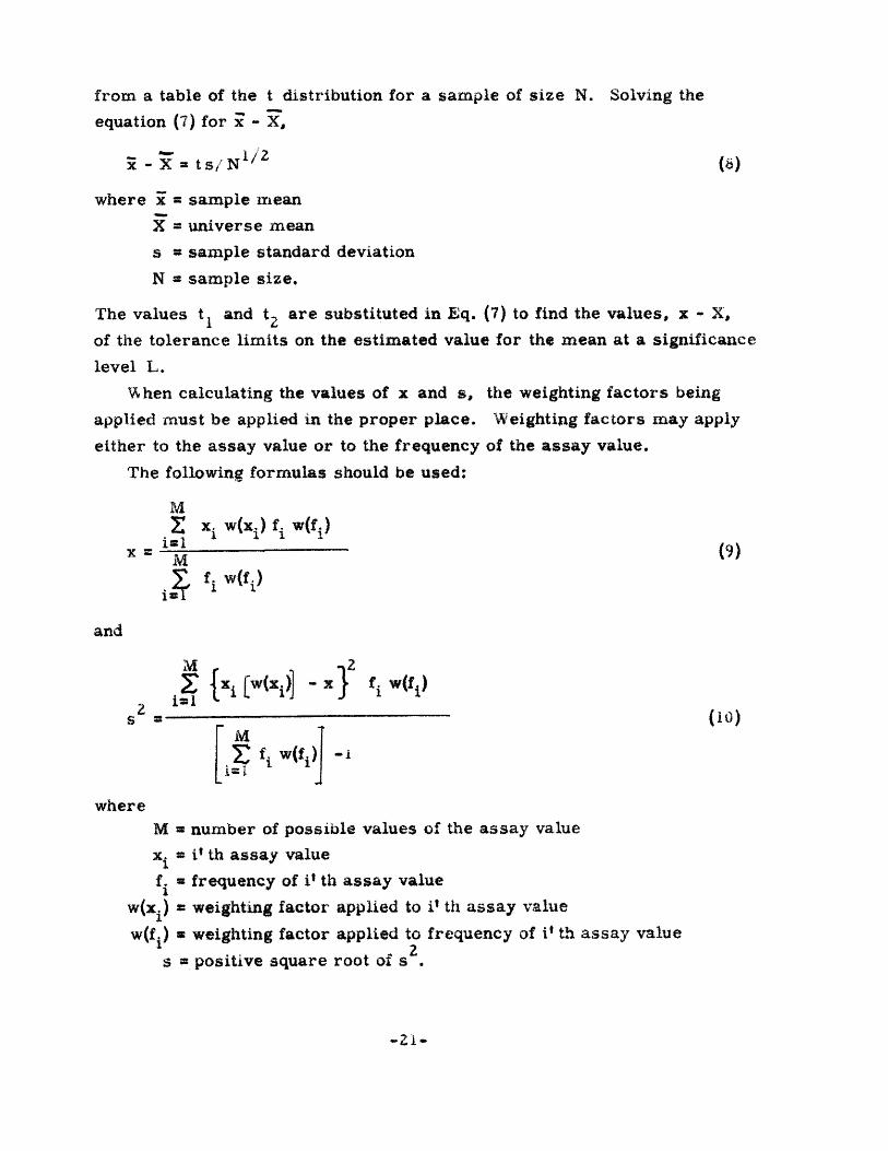
from a table of the t distribution for a sample of size N. Solving the

equation (7) for - X,

R - X = ts/N ' (8)

where x = sample mean

X = universe mean

s = sample standard deviation

N = sample size.

The values tl and t 2 are substituted in Eq. (7) to find the values, x - X,

of the tolerance limits on the estimated value for the mean at a significance

level L.

When calculating the values of x and s, the weighting factors being

applied must be applied in the proper place. Weighting factors may apply

either to the assay value or to the frequency of the assay value.

The following formulas should be used:

M

x - M (9)x= iM

Z fi w(fi)1=1

and

M 2S w(xi)] - x f w(f 1 (o)

fi w(f) -i

whereM = number of possible values of the assay value

x = i' th assay value

fi = frequency of i' th assay value

w(xi) = weighting factor applied to i' th assay value

w(fi) = weighting factor applied to frequency of i' th assay value

s = positive square root of sa

-21-

The denominator of 9 and 10 is the generalized form of the sample size and,if it is not equal to N, it should be used in place of N in all calculations in-volving s or .

An Example of the Use of the "t" Distribution.

To illustrate the use of the procedure described above and to investigatecertain characteristics of the results, the test was used on four samples ofdifferent sizes drawn from the iron deposit described in Appendix A. Theresults of this analysis are not as close to the production figures for thedeposit as would be desired, but this is probably because the cut-off limitsof the ore body as determined by the mining company were not clear insome places, and the samples included in this analysis may not be entirelytaken from the part of the deposit mined as ore.

The analysis of a sample composed of alternate drill holes along thenorth-south coordinates on the map in Appendix A will be described indetail. The majority of the drill cores from this deposit were divided intofive foot sections for analysis; and for that reason, the sample unit usedin the calculations was a five foot section of drill core. The average assayvalue of each drill hole was computed, and each value was weighted by thenumber of five foot sections in the length of the corresponding hole. Thesame results could have been reached by treating each five foot sectionseparately, but the calculations would have been less easily mechanized.Table III shows the form of the calculations for this sample. For a sig-nificance level of 95 percent

t l = -1.96

t = +1.96

then

(i - X) 1.96 (3.054)/24.94 = .239

(i - X)2 = -1.96 (3. 054)/24. 94 a -. 239,

and the average assay value of the deposit is estimated as 58. 75 . . 24 to asignificance level of 95 percent.

An Evaluation of the Procedure and its Variations.

The only error possible in the actual statistical procedure described

above is that of accepting the tolerance limits on the mean assay value

when this value is actually outside of the tolerance limits. If the sample

is taken in such a way that it is a reasonably unbiased sample, the level

of significance determines the probability of making this error. The

geologic hypothesis which is to be accepted or rejected on the basis of

the results of the analysis is usually the hypothesis that the average grade

of the deposit is above the minimum commercially valuable limit. If the

whole tolerance interval for the mean is above or below the commercial

border value, the hypothesis is respectively accepted or rejected. The

values of tl and t. were chosen such that the probability that the mean

is outside the tolerance interval on the low side is equal to the probability

that it is outside on the high side, and the probability of either is (i - L)/2

where L is the significance level chosen. The maximum probability of

errors of the first or second kind occur in that order when the upper or

lower limit of the tolerance interval is on the commercial limit. In each

case the probability of being out of the tolerance limit on the side that

corresponds to the commercial cut-off limit is the probability of the cor-

responding error and is (I - L)/Z. Thus, if the tolerance interval on the

mean is entirely above or entirely below the commercial cut-off limit,

then the maximum probability of an error of the first kind is equal to the

maximum probability of an error of the second kind and is (I - L)/2. If

the commercial cut-off limit is inside the tolerance interval on the mean

assay value, the probability of an error can be found by determining the

confidence level, L , such that the tolerance interval corresponding to

L* is entirely above or below the cut-off limit. The maximum probability

of an error is then (I - L*)/Z.

If there is reason to prefer a higher probability of one kind of error

than of the other, the values of t I and t 2 can be determined so that the

probability of t being below tI is not equal to the probability that t will

be above t2 . In any case the sum of the probability of being above t 2

and the probability of being below t I is I - L.

-23-

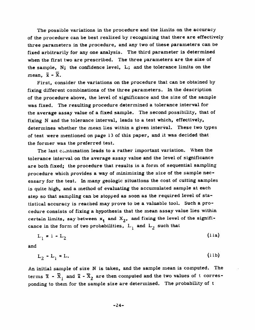
The possible variations in the procedure and the limits on the accuracy

of the procedure can be best realized by recognizing that there are effectively

three parameters in the procedure, and any two of these parameters can be

fixed arbitrarily for any one analysis. The third parameter is determined

when the first two are prescribed. The three parameters are the size of

the sample, N; the confidence level, L; and the tolerance limits on the

mean, -" X.

First, consider the variations on the procedure that can be obtained by

fixing different combinations of the three parameters. In the description

of the procedure above, the level of significance and the size of the sample

was fixed. The resulting procedure determined a tolerance interval for

the average assay value of a fixed sample. The second possibility, that of

fixing N and the tolerance interval, leads to a test which, effectively,

determines whether the mean lies within a given interval. These two types

of test were mentioned on page 13 of this paper, and it was decided that

the former was the preferred test.

The last cm.nbination leads to a rather important variation. When the

tolerance interval on the average assay value and the level of significance

are both fixed; the procedure that results is a form of sequential sampling

procedure which provides a way of minimizing the size of the sample nec-

essary for the test. In many geologic situations the cost of cutting samples

is quite high, and a method of evaluating the accumulated sample at each

step so that sampling can be stopped as soon as the required level of sta-

tistical accuracy is reached may prove to be a valuable tool. Such a pro-

cedure consists of fixing a hypothesis that the mean assay value lies within

certain limits, say between x1 and X 2 , and fixing the level of the signifi-

cance in the form of two probabilities, LI and L such that

LI - L2 (I 1a)

and

LZ - L 1 = L. (lb)

An initial sample of size N is taken, and the sample mean is computed. The

terms 3 - X I and i - X 2 are then computed and the two values of t corres-

ponding to them for the sample size are determined. The probability of t

-24-

falling in the interval between the two calculated values of t can be found

from a table of the t distribution for the appropriate size of the sample

taken; and, if this probability is between L and L 2 , the size of the

sample is increased; and the procedure is repeated for the new sample

size. If the probability of t being between the two calculated values is

less than L 1 , the sampling is over; and the hypothesis is rejected. If

the probability that t is between the calculated values is greater than L. ,

the sampling is stopped; and the hypothesis is accepted. It has not been

proven that the probability that t is within the calculated interval will

ever become less than L 1 or greater than L 2, and an attempt to get too

high a significance level, L, may result in a sample sequence that never

terminates.

The affect of a change in one of the parameters or a second parameter

when the third is held fixed provides a basis for investigating the effect of

an increase in the required accuracy of the tolerance interval or signifi-

cance level. Consider, first, the case in which the level of significance

is held fixed. The level of significance determines the value of t and the

tolerance limits are then given by

S- Rax c/N 1/ 2 (ca ts = constant) (i2)

The tolerance limits are seen to be inversely proportional to the square

root of the sample size for a fixed significance level. In order to halve

the tolerance interval the sample size should be increased by a factor of

four, for example. Of course, the relationship is not that simple because

x is related to N in a random fashion, but the above relationship still

indicates the order of magnitude of the sample increase as a function of

the decrease in tolerance limits. The effects of the significance level on

the tolerance limits and sample size are not so obvious. The effect of the

significance level on the tolerance interval can best be seen from a plot of

the cumulative distribution of t for the fixed sample size (figure 9). Since

the tolerance interval is directly proportional to t, a plot of the tolerance

interval against the significance level has the same shape as the t distri-

bution. The important part of the curve is that part that corresponds to

high significance levels. For example, to halve the probability of an error

-25-

from a significance level of . 95 requires that the tolerance interval be in-

creased by a factor of about . 19, assuming a sample size of 40. Thus,

small changes in the required tolerance interval may cause large changes

in the probability of making an error. The square root of the sample size

is also proportional to t so that the probability of making an error (1 - L)

is even more sensitive to changes in N than to changes in the tolerance

limits for high levels of significance.

A more realistic example of the interaction of the three parameters

may be found by actually calculating the tolerance limits of the mean assay

value of a deposit for varying sample sizes. Estimates of the mean of the

iron content of the deposit described in Appendix A were computed for four

sample sizes with the following results:

Sample Size Estimated Mean

320 60.44 t .25

622 58.76 + .24

812 59.18 .184

1103 58.96_+ .176

The last three samples are seen to be converging to a value of about 59. 00

at a rate that is indicated by the tolerances, but the first value is obviously

incorrect. The drill holes used in the first sample were the holes used as

a preliminary sample (holes with numbers from I to 2 i on the map in

Appendix A), and they may not be a representative sample of the deposit.

It may be noticed that the ratio of the size of the second to the size of the

fourth samples is slightly under a factor of two, and the corresponding

change in the tolerance limits is slightly under the square root of two.

Thus, the experimental results are quite close to the theoretical results

for a change in the sample size, and the estimated average seems to be

converging to a value of about 59.

VI. SEQUENTIAL ANALYSIS

In the last twenty years, a statistical procedure known as "SequentialAnalysis," designed to be used for testing hypotheses concerning one ormore parameters from a distribution of a known form, has oeen developed.10The methods of Sequential Analysis have several advantages over most otherprocedures for the type of statistical analysis needed for geologic samples.The desired probabilities of errors of the first and second kind enter into

the procedure explicitly; the procedure is, as the name implies, a sequentialsampling procedure; the procedure has required as few as half the number

of samples needed by other methods of analysis for the same statistical

accuracy; and the amount of information that can be used in this test is quite

flexible after the minimum amount of information for using the procedure

is available. Obviously, there must be a limit to the statistical accuracy

that can be obtained for a given amount of information or to the minimum

number of samples that must be taken to reach a given level of significance.

The savings in the number of samples used by the Sequential Analysis pro-

cedures may be due, in part, to the ability of the test to use a more flexible

amount of information than many other tests by allowing all of the known

parameters of a distribution to be used in estimating the unknown parameters.

To use the Sequential Analysis procedure, the two constantsA 2---

and

13 b

where

a = the probability of an error of the first kind

P = the probability of an error of the second kind

are computed. Next, the values of the wsequential probability ratio," P iP 0(where P is the probability of getting the latest sample if the hypothesis is

true and P I is the probability of getting the latest sample if the hypothesis Is

false), is computed for the latest sample.

-27-

P1' PO < A, the hypothesis is accepted.

A < P1iPo < B, the sample size is increased and the new P I/Pis tested.

B < P /PO, the hypothesis is rejected.

The Application of Sequential Analysis Based on the Distribution of the

Sample Universe.

Unless the distribution of the universe being sampled is known in analytic

form (and even in some cases when it is known) the calculation of P0 and P1may be quite difficult. The calculation of the sequential probability ratio

for a sample from a geologic deposit, for example, could be computed as

follows:

Let M = number of possible assay values,

Ak k'th possible assay value (k = i to M),

P(Rk) = percentage of the total number of sample units in the

deposit with a value Rk,

N = Sample size.

The probability of getting any given sample of N sample units

R , , ... Rk (each k may take any value from 1 to M)

is of the form* N Pn(l) )

__ POIYl N(t22). N(RM)

= I NR))! N(R Z) ! ... N(RM)!

(13)

where N(itk) = number of times Rk appears in the sample.

The hypothesis to be tested is in the form of stated limits on the M values

of the probabilities of the M possible assay values. The probability P1 is,

now, the sum of probabilities of the form of Eq. ( 3) for all possible combi-

nations of the P(Rk)' s that will make the hypothesis false; and the proba-

bility P0 is the sum of the probabilities of the form of Eq. (13) for all

-28-

possible combinations of the P(dk)' s for which the hypothesis is true.

Thus, the calculations involved in computing the sequential probability

ratio at each step of the sample would involve computing the multinomial

probability stated above for all M possible values of the N percentages

P(Rk), a total of MN times in all. If the assay values were carried onlyto the nearest . I percent, M would be 1000; and the sample size would

surely be greater than, for example, 20 and would increase at each step.

Thus, on the order of 100020 computations of Eq. (13) would be required

at each step. Even using the fastest electronic calculators in existence

this would take on the order of 10 years.

These calculations could be simplified by placing restrictions on the

allowable values of the P(Rk)' s and by making approximations in Eq. (13).

However, until more dependable information is available about the distri-

butions of geologic samples the use of Sequential Analysis procedures based

on the distribution of the sample will be of no practical value.

Application of Sequential Analysis Based on the "t" Distribution.

A more practical approach to the use of the procedure of Sequential

Analysis may be to use a combination of multiple and sequential sampling

techniques. If the hypothesis tested is in the form of a statement that the

average of the sample means for samples of size N is within a certain

interval and the sample size, N, is large enough that the sample mean

can be assumed to have a "t" distribution, the sequential probability

ratio may be relatively easy to calculate. -When the test indicates that

the sample being tested should be larger, another sample of size N must

be taken; and its mean is included in the computation of the next sequential

probability ratio. This approach may not be of much value if many sample

units are needed because each sample unit is the mean of a geologic sample

of size N, and N must be large enough that the "t" distribution is valid.

Thus, the number of geologic samples needed increases rapidly with each

step of the analysis and final number of geologic samples may be much

higher for this sequential test than for a fixed sample method such as the

one described in Section V. On the other hand, this method may terminate

rapidly and may prove to be extremely efficient; it certainly merits a more

thorough study.

VII. SUMMARY

Geologic sampling must serve many purposes, and the procedures ofmathematical statistics can be applied to only a few of them. However,

when statistical procedures are applicable, they should provide reliableand efficient techniques for getting as much information as possible from

as few samples as possible.

Statistical methods cannot be applied to any collection of samples with-out regard to their origin. If statistical concepts are to be used in ana-lysing the samples, they must also be used in collecting and weightingthem in order that the samples will be statistically representative of thedeposit from which they are taken.

In order to get the most accurate and efficient results from a statistical

analysis all available valid information about the distribution of the depositbeing sampled should be incorporated into the analysis. The procedures

discussed in this paper were based on the rather sketchy and incompleteknowledge now available concerning the nature of the distribution fromwhich samples of geologic deposits are drawn. As our understanding ofthe statistical properties of mineral deposits becomes more complete,

more efficient procedures of statistical analysis will become applicable

to geologic problems. The procedures which seem to offer the most valu-

able potentialities are those that allow sequential sampling of the deposit

being analysed, and the most important of these is the method known as

"Sequential Analysis. "

-30-

Table I

Calculations for

on Line 500W of the

test of randomness of samples from north to south

deposit described in Appendix A.

Hole Number

543

552

549

468

460

416

415

1B

13

538

AverageAssay Value

60.60

62.04

62. 65

60.13

63.90

61.37

59. 12

61.76

60. 17

56.29

x - xSign of

x-Median

+I.

-3.

+4.

Table II

Tables for the test of randomness of a series at a significance level

of . 95 based on the length of the longest run in the series.

Size of Sample Minimum Length of Run for anIndication of a Non-Random Series.

Table III

Calculations for estimating the average assay value of the deposit in

Appendix A from a sample of composed alternate drill holes in the north-

south lines.

HoleNumber

26

555

453

452

546

451

419

538

1B

11

4

519

6

409

903

413

493

533

461

463

460

549

543

537

Average Valueof Hole (x)

62.42

49.91

61.25

60.40

58.29

60. 57

61.5 S

56.29

61.76

61.79

63.52

59.99

59. 17

57.96

56.68

57.22

55.57

53.58

63.00

62.26

63.90

62.65

60. 60

56. 91

-32-

Number of SampleUnits in Hole (f)

20

20

30

20

25

34

15

29

35

17

6

33

37

40

31

13

16

21

15

14

1

12

10

18

(x - i)

13.396

78.323

6.200

2.69

.221

3.276

7.563

6.101

9. 000

9. 181

22.658

1.513

.168

.640

4.326

2. 372

10. 176

26.832

17.978

12.250

26.420

15. i32

3. 3863.423

Table III (continued)

Average Valueof Hole (x)

56.03

62.02

61.71

61.65

54. 71

58.53

54.28

55.92

59.02

60.54

Number of SampleUnits in Hole (f)

4

5

8

HoleNumber

547

558

467

544

534

900

531

505

- fxx = = 58.759

s = (X= 9. 325Ef

N1/2 = (zf)1/2 =24.940

Estimated average assay value 7+ 1. 96 (siN ) 'N 58.759 + .240.

-33-

(x - 1)2

7.453

10.628

8.703

8. 352

16.403

.053

16.403

8.066

.068

3. 168

FIGURES

Figs. 1, 2 Examples of log-normal geologic frequencydistribution.

Fig. 2

Figs. 3, 4

Fig. 4

Fig. 5

Figs. 6, 7, 8

Fig. 7

Fig. 8

Fig. 9

Cumulative Distribution of the logarithmsof the distributions in Figs. I and 2 plottedon normal probability paper.

Comparison of the frequency distribution oftrench samples with those of drill samplesfrom a barite deposit.

Examples of geologic frequency distributionsthat are not log-normal.

Cumulative distribution of " t' .

Sample pattern for the iron deposit used forthe examples (in Appendix A).

Frequency distribution of the samples fromthe iron deposit used for the examples(in Appendix A).

Cumulative distribution of the samples fromthe iron deposit used for the examples(in Appendix A).

-34-

Fig.

Fig.

40

41

42

Fig. 12

44

45

46

Fig

ure

1.

Dis

tribu

tion

o

f co

pn

er

in a

eo

nta

ct

metam

orrh

ic

dero

sit.

L\

1 0

dl

of

-35-

B'igure 2.

Distribution of

sulnhur in a laterttic

den

osit,

L

U.I

,V

0.01

20

1069

99

'"-T

T

--,I

tt

I d-ti

t

747:

- -i-i

-1i

i --

j-~

-i~

'iii

-i

tt

4-w

--T

im

-4

--

t-d-

ii

4.

IJ

T

ta~

_TFIT-

r TT

-

i '

i--i

< _

-i

-t-

tii4

-1

-1

--1 _

_T__

T

.LV

~tL

iT

- _

Tt

TT

r--

ii iIF

t L

i Li1

ijj.,

VJi

i01

00

0.1

TV

It

tt

-IiJ

-:

-I ,

i i

1 i - L

, ff

i I

f t

I

1

low

t

i-t

L

T --- ----

i i

t---

~--~

I-

i

r -.

- i

~i.-

i i

.~

i i

I :r

_ i-

-t

i Fi

Ll

t-01

0.5

.1

02

.5

1 1

2 3

0 0

0 0

8090

95

9

9 9.5

9.8

999

9

99

0.

95

90

80

70

60

50

40

30

0.,,

21

0.5

0.2

0.1

0.05

9_9 99_8

99.5

99

98

80

70

60

50

40

30

20

--

,T--

- -

.T .

-.

.. -t

:

AT

t-

Eli

I

4 i

-- -

H --

-r

---1

-.-

-

FdI

-14W~'

44-v

14' ti

~i ij

IL

14-t

t[---

--

, ,-

I ,

--r-

-i -

-

.Et-

--

Ht t

_ -

--

_-

_ -

_,-i-

-- __

_ -T

-- t --

----i

I I

I I 1

44-4r, P

- ~

<U-4<-

I i

!!

1 [

ttzh

2E

lhzi

-i-'

tH-H

-TC

- -

T

-

~~ 'V

t i-

7

-t-I-

T

7Z

1

7.

-i-i

t---

- --

1-

r r

--i

_t

_-

-i

i-f-

Ti

Iiii

L4

_

4_

it -4

.i ii

1;

; :-

K

___

TI~

. t .

_!i

1 1

-I +

I-

I'

I I

_

+ -1

-4II

II

,'j4-

-T

T

1

1,

-1

--

R

Ei

'i-

- tr

r _

_-

I-

I I

I I

I

I /

1__1

1 1

I 1

/_11/1

1_

1_/1

1 I

I __1

1 1 I

1 r/lr

/ Il

I I

---

-

! m

!

I I

I I

-I

+!~-

----

ttt(

tfti

-ttt

titt

-+i-

$-~-

' -t

t--f

----

tf i

-t+

-ftl

-ttt

t-c-

~-t

-fft

~tf

-i-t

-f-

I ,I

, II

I

i

tt--f

-f -t~

-

L

TIT

,

-IT ,I--

'-t~

d~t

f#-

..

.. ..

f l

.,

I I

I I

I I

I ..

I I I

I

I .

I I

I I

.I

.iI

.l.

I I

I i

i i

99.9

995

90

10

52-

1

'

I

I I

i I

I

kHL

iJk__

0.01

0.

05

0.1

0.2

0.5

1

280

90

95

98

99

99

.5

99.8

99

.9

99.9

9

99.9

99

.8

99.5

99

98

0.5

0.2

0.1

0.05

0.01

I I

5 10

20

30

40

50

60

70

Figure 5.

Distributions of trench and drill samples frop a replacement

deposit of barite.FRA fsWCY

04

]F 1 FM- TH0o

Drill Samples

rFREa NCY

'Din1

60di411Th]

Trench Samples

-39-

s.0

4Af 'ri.

I1O AR ITE

- - - -- --

iinu

re

.

Distrib

utio

n

of

TiO

2in

a cla

y

denosit.

-40-

igu re

7.

Distribution of

iron in P lateritic denosit of iron

and nickel.

I

U[,,

',

'a--I-

Fi

ure

8,

Distribution of

iron in a laterite in the w

este

rn nart

of

the

Gogeb

ic range.

OO

The

cum

ula

tive

dis

tribu

tion

of

"t".

00

0

0 10

0

0C

9 q4.c'

i'irure

9.

300W 700W 500W

0555

01. i

538

0,3

f 51

011530,6

0 ,121

OIA

5 30

0903

O4 5*

O

0 54f

0375

0533

03

0 8or 1

0518

053

0211

09oo

Figure 10

Samnle pattern for the iron deposit used as an examDle in the text.

.44-

IIOOW22

2.0

300W 1OOW

)90f

I15

100E

,9,

Oqo2 0,--e Yc6

IG F-

OGA

019

01570116

NLi607

I

10

8

0373

5584L60

0 61

0163

470

54' 9

O55a552

O05

O518 90513

0902O22

0537 G O53 Ia8

0901

-r- - - - - - - - -.-- -- ,- E-MM- -------- rra M. C--1--11-11"m --- l-

t 4 - 6b

-I -

1OSL(6

0167

Fig

ure

1

1.

Freq

uen

cy dis

tributio

n

(histo

gra

m)

for

the

iron

deposit

used as

the

standard

exam

ple in

the

text.

't4

_ _t

L

Ii

-4500

Figure 12.

Cumulative distribution of the iron deposit used as

a standard example in the text.

I

00

0

0%

Q o0

vc Ew

O~32 b o

APPENDIX A

All examples used in this paper have been taken from one lateritic

iron deposit. Table IV describes the average iron content and the

length of each of the sample holes in the ore. Since this paper is not

concerned with determining cut-off limits for mining the deposit, only

the holes in the ore are described. Figure 10 is a map of the drill

hole pattern, and Figures 11 and 2 are, respectively, the frequency

distribution and cumulative distribution of the samples.

Si -

Table IV

Assay Values from an Iron Deposit

Hole Number

iAIB34A4B6A6B7

11131415222628

211373375405409413415416419421451452453457460461463464467468469470493505512514

Average AssayValues in Percent

60. 1561.7660.5463.5259.0259.1759.3165.1861.7960.1761.1462.2360.0362.4260.4154.0461.2059.8557.1657.9657.2259.1261.3761.5161.6060.5760.4061.2561.3263.9063.0062.2659.2961.7160.1359,.2350.4855.5755.9259.3956.82

Number of Five FootSample Units in Hole

1635106

103798

17403023162022213

15384013222

152434203016

11514138583

16102410

-ii -

Hole Number

515518519530531533534537538543544545546547548549552554555558900901902903904

Table IV (continued)

Average AssayValues in Percent

Number of Five FootSample Units in Hole

55.8859.1359.9958.9054.2853.5854.7156.9156. 2960.6061.6556.6258.2956.0361.6962.6562.0458.9849.9162.0258.5355.6960.0656.6845.77

- ii -

The Normal and Lognormal Distributions.

The frequency distribution of a normally distributed

variate,x, is defined as

Y(x)= -

where

r= the standard deviation

4 the mean of the distribution

Y= the frequency of the value,x,

This curve is always symmetric, but its share will vary for

different values of a- . The black curve in the figure below

is a normal frecuency distribution.

The loouormal distribution is a distribution in which the

log of the variate is normally distributed, and is always nos-

itively skewed. The blue curve in the figure below is a log-

normal frequency distribution.

iefex ences

1. Hoel, Paul G., Introduction to Mathematical Statistics, John Wileyand Sons, New York, pp. 180-81.

2. Swed, F. and Eisenhart, C., "Tables for Testing iRandomness ofGrouping in a Sequence of Alternatives," Annals of MathematicalStatistics, Vol. XIV (1943), pp. 66-87.

3. Mosteller, F., "Note on Application of Runs to Quality ControlCharts," Annals of Mathematical Statistics, Vol. XII (1941),pp. 228-232.

4. Ahrens, L. H., "The Lognormal Distribution of the Elements,"Geochimica et Cosmochimica Acta, Vol. V (1954), pp. 49-73.

5. United States Bureau of Mines Reports of Investigations Numbers3900, 3971, 4155, 4189, 4214, 4349, and 4503.

6. DeKock, W. P., "The Carbon Leader of the Far West Aiand WithSpecial Reference to the Proportion of the Gold Content of ThisHorizon Recovered in Drilling," Transactions of the GeologicalSociety of South Africa, Vol. L 1 (1949), pp. Z13-47.

7. Hoel, Paul G., Introduction to Mathematical Statistics, John Wileyand Sons, New York, pg. 68.

8. Ibid., pp. 35-36.

9. Dixon, Wilfred J. and Massey, Frank J., Introduction to StatisticalAnalysis, McGraw-Hill Book Company, Inc., New York, pp. 97~IO1,

10. Wald, A., Sequential Analysis, John Wiley and Sons, New York.

-iv-

Bibliography

1. Ahrens, L. H., "The Lognormal Distribution of the Elements,"Geochimica et Cosmochimica Acta, Vol. V (1954), pp. 49- (3.

2. DeKock, W. P., "The Carbon Leader of the Far West Rand WithSpecial Reference to the Proportion of the Gold Content of ThisHorizon Recovered in Drilling," Transactions of the GeologicalSociety of South Africa, Vol. L I (1949), pp. 213-247.

3. Dixon, Wilfred J. and Massey, Frank J., Introduction to StatisticalAnalysis, McGraw-Hill Book Company, Inc., New York, 1951..

4. Feller, William, An Introduction to Probability Theory and itsApplications, Vol. 1, John Wiley and Sons, Inc., New York, 1950.

5. Hoel, Paul G., Introduction to Mathematical Statistics, John Wileyand Sons, Inc., New York, 1947. .

6. Mosteller, F., "Note on Application of Runs to Quality Control,"Annals of Mathematical Statistics, Vol. XII (1941), pp. 228-232.

7. Parks, Roland D., Examination and Valuation of Mineral Property,Addison-Wesley Press, Inc., 1949, 3rd edition.

8. Statistical Research Group, Sequential Analysis, Columbia UniversityPress, 1945.

9. Swanson, C. O., "Probability in Estimating the Grade of GoldDeposits," Transactions of the Canadian Institute of Mining andMetallurgy, Vol. 48 (1945), pp. 323-335.

10. Swed, F. and Eisenhart, C., "Tables for Testing Randomness ofGrouping in a Sequence of Alternatives," Annals of MathematicalStatistics, Vol. XIV (1943), pp. 66-87.

11. United States Bureau of Mines Reports of Investigations Numbers3900, 3971, 4155, 4189, 4214, 4349, and 4503.

12. Wald, A., Sequential Analysis, John Wiley and Sons, Inc., New York.