A spring–dashpot system for modelling lung tumour motion...

A spring–dashpot system for modelling lung tumour motion inradiotherapy

P.L. Wilsona* and J. Meyerb

aDepartment of Mathematics and Statistics, University of Canterbury, Christchurch, New Zealand;bDepartment of Physics and Astronomy, University of Canterbury, Christchurch, New Zealand

(Received 6 August 2008; final version received 20 October 2008 )

A 3D system of springs and dashpots is presented to model the motion of a lung tumourduring respiration. The main guiding factor in configuring the system is the spatialrelationship between abdominal and lung tumour motion. A coupled, non-dimensionaltriple of ordinary differential equations models the tumour motion when driven by a 3Dbreathing signal. Asymptotic analysis is used to reduce the system to a single equationdriven by a 3D signal, in the limit of small lateral and transverse tumour motions. Anumerical scheme is introduced to solve this equation, and tested over wide parameterranges. Real clinical data is used as input to the model, and the tumour motion output isin excellent agreement with that obtained by a prototype tumour tracking system, withmodel parameters obtained by optimization. The fully 3D model has the potential toaccurately model the motion of any lung tumour given an abdominal signal as input,with model parameters obtained from an internal optimization routine.

Keywords: modelling; asymptotic analysis; numerical analysis; optimization; lung;tumour; respiration; radiotherapy

AMS Subject Classification: 92C05; 92C10; 92C50

1. Introduction

Cancer of the respiratory tract is a common disease with relatively poor prognosis. The

leading cause of death from cancer in 2004 in New Zealand was cancer of the trachea,

bronchus and lung. It ranked 3rd and 4th in terms of incidence for males and females,

respectively, and the 1- and 5-year survival is approximately 30 and 15% [9]. Radiation

therapy alone or in combination with chemotherapy and/or surgery are the main modalities

to treat cancer. One of the reasons for the unfavourable treatment response to radiation

therapy is the fact that for lesions in the lung comparatively large treatment margins are

required to account for respiratory-induced tumour motion [6]. Inevitably, this results in a

larger volume of normal tissue being irradiated, thereby considerably increasing the side

effects of the treatment. Consequently, the total tolerable treatment dose that can be given

to the tumour is lower than what is necessary for adequate tumour control.

If the exact tumour position were known at all times during irradiation, the treatment

parameters could be adjusted and hence the dose delivered more conformally [4,7]. This, in

turn,wouldmake it possible for higher overall doses to begiven to the tumour keeping the side

effects at a comparable level. In practise, it is technically difficult to directly determine the

ISSN 1748-670X print/ISSN 1748-6718 online

q 2010 Taylor & Francis

DOI: 10.1080/17486700802616534

http://www.informaworld.com

*Corresponding author. Email: [email protected]

Computational and Mathematical Methods in Medicine

Vol. 11, No. 1, March 2010, 13–26

actual tumour position non-invasively in real-time during treatment [2,11,14,15,17,18,24].

Instead,most non-invasive approacheshave resorted tomeasuring the respiratory signal of the

patient, which is ultimately related to lung tumour motion. Accurate and reliable models are

required to correlate the relationship between respiratory and lung tumour motion to ensure

that the positionof the tumour is knownat all times. Failure to determine irregular breathing or

so-called base line drift can result in inaccurate dose delivery.

A thorough description of modelling lung tissue properties taking into account

viscoelastic non-linear stress-strain behaviour can be found in Refs [19,20]. However, the

focus of this work is the spatio-temporal relationship between abdominal motion and that of

a tumour embedded in the lung tissue. Previous work investigated simple ‘grey box’ type

models of this relationship [10]. While these models were successfully applied to clinical

cases, intrinsically they do not have the ability to model certain behaviours of the tumour-

breathing signal relationship, such as when the tumour trajectory exhibits a hysteresis [17]

or when a spring-like elasticity can be observed. This is because they attempt to fit model

parameters (in a least-squares sense) to a linear (or non-linear) model, which does not

resemble the physical relationship of the data set. This is why they are referred to as ‘black

box’ models, or, if some prior knowledge is incorporated, as ‘grey box’ models.

In this work, a novel 3D model is presented, which aims to physically model the spatial

relationship between an external signal, representing abdominal breathingmotion, and a lung

tumour. The approach is based on an array of springs and dashpots arranged tomodel tumours

at any location within the lung. While the mathematical model is general for any tumour in

the lung, the parameters governing the springs and dashpots are patient- and tumour location-

specific. The characteristics of the model are analysed both mathematically and by means of

computer simulations. Finally, the model is validated against real clinical tracking data.

2. A full 3D model

2.1 Physical setup

Figure 1 shows the 3D system of springs and dashpots at a general time t*, where a

superscript star indicates a dimensional quantity. The tumour lies at position p*T ðtÞ ¼ðx*T ðt* Þ; y

*T ðt* Þ; z

*T ðt* ÞÞ where (x*, y*, z*) forms a right-handed triad as shown, with

corresponding unit vectors (i, j, k). Althoughwe have drawn the tumour lying at negative x*,

y* and z*, it will in general explore both positive and negative values of all directions. In so

doing, each spring can if necessary move through its pivot point without penalty. The

tumour is connected via spring sX of natural length l*X to a pivot point free to move in the

plane x* ¼ l*X . Dashpot dX provides damping of the x*-motion, and is likewise free to move

in a (y*, z*)-plane to track the (y*, z*)-components of the tumour position. This ‘tracking’

behaviour of the spring sX and dashpot dX is a phenomenological model of the multiple

forces acting laterally on the tumour due to multiple attachment points and lung movement.

The mechanical responses of the connective tissue are not directly modelled, but rather the

response of the tumour to diaphragm motion, resulting in abdominal movement. In this

initial approach, a serial spring–dashpot arrangement in each direction forms the basis of

the model. The tumour is also connected via a spring sZ of natural length l*Z to a pivot point

free tomove in the plane z* ¼ l*Z . Dashpot dZ provides damping of the z*-motion, being free

to move in an (x*, y*)-plane to track the (x*, y*)-components of the tumour position.

Spring sY of natural length l*Y connects the tumour to the point p*Dðt* Þwhich represents the

diaphragm. The diaphragm point p*Dðt* Þ is assumed to move only along a superior–inferior,

or sup–inf (head-to-feet), line through the origin; it is constrained to lie on the line x* ¼ 0,

z* ¼ 0. It is the diaphragm point which drives the tumour motion by means of being itself

P.L. Wilson and J. Meyer14

connected by a rigid rod of length R* to the point p*Aðt* Þ, which models the time-varying

abdominal position of the patient during breathing, and is in general 3D. Tension in the spring

sY acts only to change p*T ; the diaphragm position p*D varies only with changes in the abdomen

position p*A. Because both the tumour and abdomen each have three degrees of freedom we

call this model the 3D–3D model referring to tumour and abdomen, respectively.

(Experiments measure the abdominal motion, as described in Section 4, while diaphragm

movement is not measured experimentally.) A dashpot dY dampens the y*-motion, and is free

to move in an (x*, z*)-plane to track the (x*, z*)-components of the tumour motion.

We assume here that all springs follow Hooke’s Law, with sX, sY, sZ having stiffness

k*X ; k*Y ; k

*Z , respectively. Furthermore, we take all dashpots to provide friction proportional

to the velocity component in the relevant direction. Again, other choices could be

considered. Note that since the tumour motion is influenced by the mechanical properties

of the lung tissue, future work will, if necessary, consider more complex spring–dashpot

arrangements, non-Hookean spring behaviour, or alternative dampers.

In the next section we derive the coupled equations of motion which govern the 3D–

3D system.

2.2 Governing equations

Referring again to Figure 1, we denote by uX the angle which sY makes with the plane

x ¼ 0, and the angle which sY makes with the plane z ¼ 0 is denoted uZ. These angles can

be written in terms of the other variables. Then if the constant mass of the tumour is m*,

Newton’s second law with the assumptions of Hookean springs and the form of the

dashpot resistance gives the governing equations.

m* €x*T ¼ k*Xx*T þ k*Yj

*Y sinuX cosuZ 2 b*

X _x*T ; ð1Þ

Figure 1. The spring–dashpot system.The coordinate axes, spring and dashpot labels, and the positionof the tumour, diaphragm, and abdomen are shown. The degrees of freedom are indicated by arrows.

Computational and Mathematical Methods in Medicine 15

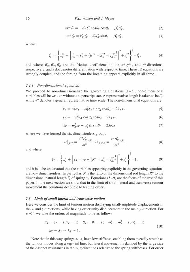
m* €y*T ¼ 2k*Y j*Y cosuX cosuZ 2 b*

Y _y*T ; ð2Þ

m* €z*T ¼ k*Z z*T þ k*Yj

*Y sinuZ 2 b*

Z _z*T ; ð3Þ

where

j*Y ¼ x*2T þ y*A 2 y*T þ R*2 2 x*2A 2 z*2A� �1

2

� �2þ z*2T

( )12

2l*Y ; ð4Þ

and where b*X ;b

*Y ;b

*Z are the friction coefficients in the x*-,y*-, and z*-directions,

respectively, and a dot denotes differentiation with respect to time. These 3D equations are

strongly coupled, and the forcing from the breathing appears explicitly in all three.

2.2.1 Non-dimensional equations

We proceed to non-dimensionalize the governing Equations (1–3); non-dimensional

variables will be written without a superscript star. A representative length is taken to be l*Y ,

while t* denotes a general representative time scale. The non-dimensional equations are

€xT ¼ v2XxT þ v2

YjY sinuX cosuZ 2 2lX _xT ; ð5Þ

€yT ¼ 2v2YjY cosuX cosuZ 2 2lY _yT ; ð6Þ

€zT ¼ v2ZzT þ v2

YjY sinuZ 2 2lZ _zT ; ð7Þ

where we have formed the six dimensionless groups

v2X;Y ;Z ¼

t*2k*X;Y ;Z

m*; 2lX;Y ;Z ¼

t*b*X;Y ;Z

m*; ð8Þ

and where

jY ¼ x2T þ yA 2 yT þ R2 2 x2A 2 z2A� �1

2

� �2þ z2T

( )12

21; ð9Þ

and it is to be understood that the variables appearing explicitly in the governing equations

are now dimensionless. In particular, R is the ratio of the dimensional rod length R* to the

dimensional natural length l*Y of spring sY. Equations (5–9) are the focus of the rest of this

paper. In the next section we show that in the limit of small lateral and transverse tumour

movement the equations decouple to leading order.

2.3 Limit of small lateral and transverse motion

Here we consider the limit of tumour motion displaying small-amplitude displacements in

the x- and z-directions, while having order unity displacement in the main y-direction. For

1 ! 1 we take the orders of magnitude to be as follows

xT , zT , 1; yT , 1; uX , uZ , 1; v2X , v2

Z , 1;v2Y , 1;

lX , lY , lZ , 1:ð10Þ

Note that in this way springs sX, sZ have low stiffness, enabling them to easily stretch as

the tumour moves along a sup–inf line, but lateral movement is damped by the large size

of the dashpot resistances in the x-, z-directions relative to the spring stiffnesses. For order


unity times, and for order unity values of all three components of the abdominal signal (so

that the signal is still fully 3D), we expand as follows

xT ¼ 1x1 þ 12 x2 þ Oð13Þ; ð11Þ

yT ¼ y0 þ 1y1 þ Oð12Þ; ð12Þ

zT ¼ 1z1 þ 12 z2 þ Oð13Þ: ð13Þ

Formally, we should also expand the spring angles and model parameters in line with

Equation (10). Here, we simply take

uX ¼ 1QX ; uZ ¼ 1QZ ; ð14Þ

v2X ¼ 1V2

X ;v2Z ¼ 1V2

Z ; ð15Þ

where QX; Z , VX; Z , 1:The leading order balances of Equation (5) (to O(1)), Equation (6) (to O(1)), and

Equation (7) (to O(1)) are

€x1 ¼ v2Y yA 2 y0 þ R2 2 x2A 2 z2A

� �12

��2 1

� �QX 2 2lX _x1; ð16Þ

€y0 ¼ 2v2Y yA 2 y0 þ R2 2 x2A 2 z2A

� �12

��2 1

� �2 2lY _y0; ð17Þ

€z1 ¼ v2Y yA 2 y0 þ R2 2 x2A 2 z2A

� �12

��2 1

� �QZ 2 2lZ _z1: ð18Þ

The main point is that Equation (17), governing the order unity motion in the y-

direction, has effectively decoupled from the other equations, in that Equation (17) can be

solved – subject to a known abdominal breathing signal – independently for y0. This

solution can then be inserted into Equations (16,18), which can be solved separately

should lateral and transverse corrections of O(1) be required. A higher-order balance of

Equation (6) would give y1, an O(1) correction to the motion in the y-direction.

In clinical settings the amplitude of tumour motion in the y-direction is typically

significantly larger than that in the x- and z-directions [17]. For this reason we take the

analysis of this section to support our work in the subsequent sections, which concentrate

on a 1D–3D model. This refers to solving the one-dimensional Equation (17) subject to a

fully 3D abdominal breathing motion. Physically, the solution of this model is the

dominant component of the fully 3D tumour motion in the limit of small lateral and

transverse displacements.

First, in Section 3, we validate the numerical approach by comparing sample data with

analytical predictions obtained by taking limiting cases of the key parameters in Equation

(17). In Section 4 we will use a numerical scheme to solve Equation (17) with patient-

specific parameters determined by an optimization routine.

3. Analytical validation of the numerics

3.1 The 1D–3D model

For clarity we reiterate that Equation (17) governs the dominant tumour motion, along the

sup–inf line, driven by a full 3D and time-dependent signal from the abdomen motion


(xA, yA, zA). The abdomenmotion is used because external tracking of it is relatively easy, as

opposed to the difficulty of obtaining real-time measurements of the diaphragm position.

Our task in this section is to show analytically that this equation has physically

reasonable solutions under certain circumstances (or limiting parameter ranges), or that

under those circumstances predictions can be made which agree with numerical solutions.

Since in a phenomenological and non-dimensional model of this kind we have no a priori

notion of ‘large’ and ‘small’ values of the key parameters, a feel for the size of these

parameters will also be obtained here. This work jointly provides confidence in the model

and in the numerical approach.

Numerical modelling was carried out in Matlab (Mathworks, Natick, MA, USA). In

this testing section of the paper, we generate a realistic but simplified breathing signal; real

clinical data is used in Section 4. The z-component of the respiratory signal was simulated

by the Weibull distribution [21] given by

zAðtÞ ¼s

h

T 2 g

h

� �s21

e2T2gh

� �s

ð19Þ

for tmodulo 4, and where h is a scale parameter, s is a shape (or slope) parameter, and g is

a location parameter. A representative respiratory signal was found for s ¼ 4,h ¼ 2 and

g ¼ 0 and will be used throughout Section 3. For convenience, xA and yA were set to zero.

Since for this section we set the ratio R to be unity, we must take zA # 1 otherwise

Equation (17) is violated. (This is a minor aspect of the non-dimensional model – future

clinical developments of the model will be dimensional.) Therefore, zA was scaled and

offset such that the respiratory signal was in the appropriate range. The scaled respiratory

signal was applied to Equation (17) as the driving term, and the equation was solved with

an in-built Matlab function for non-stiff differential equations [3].

3.2 Analysis of the 1D–3D model

The key physical parameters are the dimensionless group v2Y representing the spring

stiffness, and the dimensionless group lY representing the damping coefficient. The relative

orders of magnitude of these terms, and of the tumour motion y0 are examined as follows.

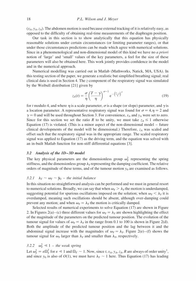
3.2.1 lY , vY , yy€y0 – the initial balance

In this situation no straightforward analysis can be performed and wemust in general resort

to numerical solutions. Broadly, we can say that whenvY . lY the motion is underdamped,

suggesting potential for spurious oscillations imposed on the solution; when vY , lY it is

overdamped, meaning such oscillations should be absent, although over-damping could

prevent any motion; and when vY ¼ lY the motion is critically damped.

Selected results of numerical experiments to solve Equation (17) are shown in Figure

2. In Figures 2(a)–(c) three different values for vY ¼ lY are shown highlighting the effect

of the magnitude of the parameters on the predicted tumour position. The evolution of the

tumour signal for values of vY ¼ lY in the range from 0.1 to 100 is shown in Figure 2(d).

Both the amplitude of the predicted tumour position and the lag between it and the

abdominal signal increase with the magnitudes of vY ¼ lY. Figure 2(e)–(f) shows the

tumour signal for vY larger than lY and smaller than lY, respectively.

3.2.2 v2Y ! 1 – the weak spring

Let v2Y ¼ 1V2

Y for 1 ! 1 andVY , 1. Now, since t, xA, yA, zA, R are always of order unity1,

and since y0 is also of O(1), we must have lY , 1 here. Thus Equation (17) has leading


order balance

€y0 þ 2lY _y0 ¼ 0; ð20Þ

which has the general solution

y0 ¼ Ae22lY t þ B ð21Þ

for constants A;B [ R dependent on the initial conditions. This suggests that y0 ! B

for large times, as is seen to occur in the numerical solution of Equation (17) shown in

Figure 2. Numerical solutions of Equation (17) for different values of vY¼lY in (Figures 2(a)–(d)), vY.lY in (Figure 2(e)), and for vY,lY in (Figure 2(f)). The blue line represents the abdominalrespiratory signal zA and the red line the leading order sup–inf tumour position y0. For comparisonthe respiratory signal is superimposed on the tumour signal such that �zA ¼ 0.


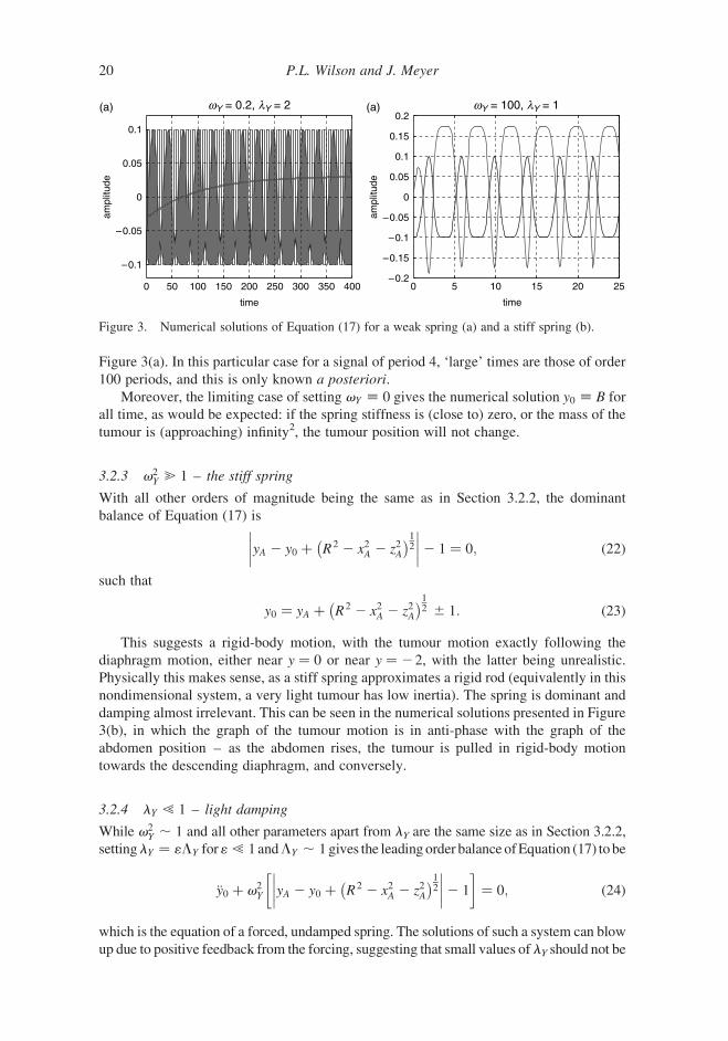
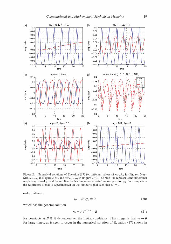
Figure 3(a). In this particular case for a signal of period 4, ‘large’ times are those of order

100 periods, and this is only known a posteriori.

Moreover, the limiting case of setting vY ; 0 gives the numerical solution y0 ; B for

all time, as would be expected: if the spring stiffness is (close to) zero, or the mass of the

tumour is (approaching) infinity2, the tumour position will not change.

3.2.3 v2Y @ 1 – the stiff spring

With all other orders of magnitude being the same as in Section 3.2.2, the dominant

balance of Equation (17) is

yA 2 y0 þ R2 2 x2A 2 z2A� �1

2

��2 1 ¼ 0; ð22Þ

such that

y0 ¼ yA þ R2 2 x2A 2 z2A� �1

2 ^ 1: ð23Þ

This suggests a rigid-body motion, with the tumour motion exactly following the

diaphragm motion, either near y ¼ 0 or near y ¼ 22, with the latter being unrealistic.

Physically this makes sense, as a stiff spring approximates a rigid rod (equivalently in this

nondimensional system, a very light tumour has low inertia). The spring is dominant and

damping almost irrelevant. This can be seen in the numerical solutions presented in Figure

3(b), in which the graph of the tumour motion is in anti-phase with the graph of the

abdomen position – as the abdomen rises, the tumour is pulled in rigid-body motion

towards the descending diaphragm, and conversely.

3.2.4 lY ! 1 – light damping

While v2Y , 1 and all other parameters apart from lY are the same size as in Section 3.2.2,

settinglY ¼ 1LY for1 ! 1 andLY , 1 gives the leadingorder balance ofEquation (17) tobe

€y0 þ v2Y yA 2 y0 þ R2 2 x2A 2 z2A

� �12

��2 1

� �¼ 0; ð24Þ

which is the equation of a forced, undamped spring. The solutions of such a system can blow

up due to positive feedback from the forcing, suggesting that small values of lY should not be

Figure 3. Numerical solutions of Equation (17) for a weak spring (a) and a stiff spring (b).


chosen in the numerical routine (although itmaybe admissible to allowO(1) values oflY such

that lY ! v2Y ). Although the solution shown in Figure 4(a) does not blow up, large spurious

oscillations occur due to the underdamping.

3.2.5 lY @ 1 – heavy damping

With all other orders of magnitude as in Section 3.2.4, the dominant effect is _y0 ¼ 0: no

tumour motion (to leading order). This is seen in numerical solutions shown in Figure 4(b),

and is to be expected, since very heavy resistance to motion, or a very light tumour with

O(1) resistance3, effectively prevents the tumour from moving.

Having gained some confidence in both the model and the general numerical approach,

we proceed in Section 4 to model real tumour trajectories obtained from clinical data.

4. Applying the model to clinical patient data

4.1 The data-collection process

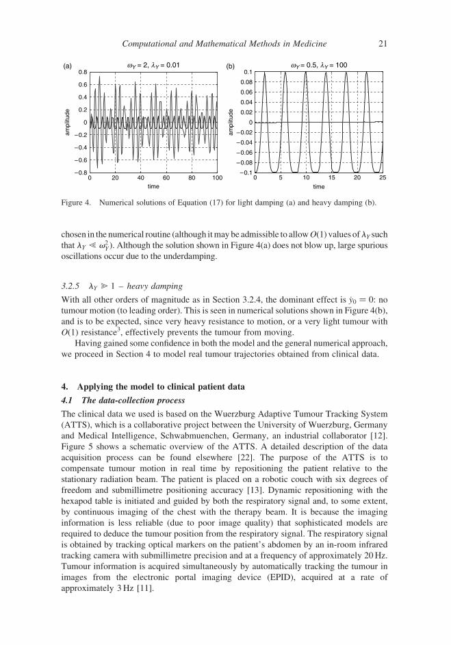
The clinical data we used is based on the Wuerzburg Adaptive Tumour Tracking System

(ATTS), which is a collaborative project between the University of Wuerzburg, Germany

and Medical Intelligence, Schwabmuenchen, Germany, an industrial collaborator [12].

Figure 5 shows a schematic overview of the ATTS. A detailed description of the data

acquisition process can be found elsewhere [22]. The purpose of the ATTS is to

compensate tumour motion in real time by repositioning the patient relative to the

stationary radiation beam. The patient is placed on a robotic couch with six degrees of

freedom and submillimetre positioning accuracy [13]. Dynamic repositioning with the

hexapod table is initiated and guided by both the respiratory signal and, to some extent,

by continuous imaging of the chest with the therapy beam. It is because the imaging

information is less reliable (due to poor image quality) that sophisticated models are

required to deduce the tumour position from the respiratory signal. The respiratory signal

is obtained by tracking optical markers on the patient’s abdomen by an in-room infrared

tracking camera with submillimetre precision and at a frequency of approximately 20Hz.

Tumour information is acquired simultaneously by automatically tracking the tumour in

images from the electronic portal imaging device (EPID), acquired at a rate of

approximately 3Hz [11].

Figure 4. Numerical solutions of Equation (17) for light damping (a) and heavy damping (b).


4.2 Preprocessing of the clinical data

The conventions of the physical model as shown in Figure 1 are such that the tumour

oscillates around the origin. The location of the respiratory signal is some distance away in

the direction of the negative y-axis. In order to apply the dimensionless equations to the

clinical data some scaling, offsetting and resampling of the raw data was required. For

example, the term ðR2 2 x2A 2 z2AÞ in Equation (17) must be positive, and so the respiratory

signal had to be scaled down. As a consequence the model output, namely the amplitude of

the tumour trajectory, was restricted to certain values requiring the tumour trajectory to be

scaled as well. The clinical data set selected was that of a patient during stereotactic lung

radiotherapy treatment [23]. To demonstrate the principle, we chose a patient who exhibited

regular breathing with a tumour which was relatively ‘visible’ in the portal images. The

main direction of abdominal movement was in the z-direction, and the main direction of the

tumour motion was in the y-direction, as shown in Figure 6. The tumour movement

displayed only small lateral and transverse motion, a requirement of the 1D–3D model.

4.3 Results of modelling the clinical data

As mentioned previously, the model equations are generic for modelling the relationship

between abdominal motion and the lung tumour position. Differences in the dynamics of

the tumour motion may originate from a number of different reasons, such as the tumour

location or the breathing technique of a particular patient. The spring–dashpot system can

model this by means of adjusting the dimensionless spring stiffness v2Y and the value of the

dimensionless damping factor lY of the dashpot. Also, the ratio of l*y and the rod length R*,

i.e. R, has an impact on the amplitude of the model output.

Figure 5. A sketch of the Wuerzburg Adaptive Tumour Tracking System, indicating the dataacquisition process. The abdominal respiratory signal is acquired with an infra-red (IR) stereo real-time tracking camera and the tumour signal is obtained by tracking the tumour in portal images [11].


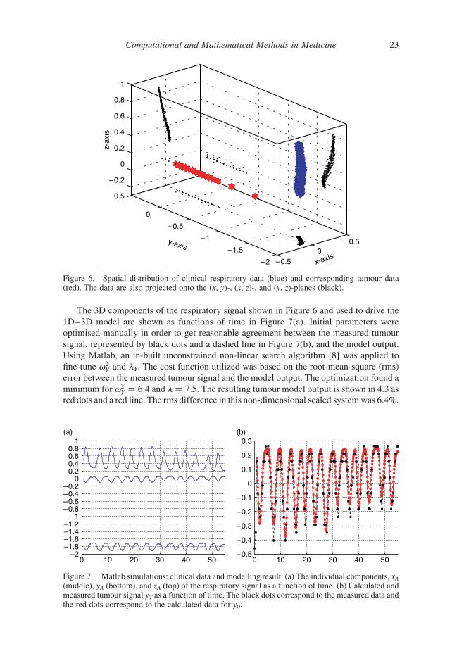
The 3D components of the respiratory signal shown in Figure 6 and used to drive the

1D–3D model are shown as functions of time in Figure 7(a). Initial parameters were

optimised manually in order to get reasonable agreement between the measured tumour

signal, represented by black dots and a dashed line in Figure 7(b), and the model output.

Using Matlab, an in-built unconstrained non-linear search algorithm [8] was applied to

fine-tune v2Y and lY. The cost function utilized was based on the root-mean-square (rms)

error between the measured tumour signal and the model output. The optimization found a

minimum for v2Y ¼ 6:4 and l ¼ 7:5. The resulting tumour model output is shown in 4.3 as

red dots and a red line. The rms difference in this non-dimensional scaled systemwas 6.4%.

Figure 6. Spatial distribution of clinical respiratory data (blue) and corresponding tumour data(red). The data are also projected onto the (x, y)-, (x, z)-, and (y, z)-planes (black).

Figure 7. Matlab simulations: clinical data and modelling result. (a) The individual components, xA(middle), yA (bottom), and zA (top) of the respiratory signal as a function of time. (b) Calculated andmeasured tumour signal yT as a function of time. The black dots correspond to the measured data andthe red dots correspond to the calculated data for y0.


The results indicate that the spring–dashpot approach is indeed capable of closely

modelling the correlation between clinical abdominal motion and measured tumour

position. The 1D–3D model parameters can automatically be optimized using a simple

cost function. In clinical terms, there are two important aspects of the model output to

consider: the lag and the signal local extrema. A persistent phase shift, or lag, between the

model output and the measured tumour signal would lead to a systematic tracking error,

inevitably resulting in underdosing of the tumour during radiotherapy treatment. Figure

7(b) shows that there is excellent agreement between the phase of both signals.

By contrast, small disagreements at the local extrema have considerably less impact on

tumour dose due to the short residency time of the tumour close to local extrema. In Figure

7(b), minor differences can be seen between some of the local extrema of the two signals

which are likely to have minimal impact [5,16]. It should also be noted that the sample

data from the ATTS are based on automatic tracking of the tumour position in portal

images. [1] discussed the technical details of the image acquisition process. In particular, it

is obvious that a low sampling rate of tumour position introduces some error, which is

likely to be worse when a local extremum falls between two sampling points. The data

from the ATTS used in this work were based on a sampling rate of 3Hz for the tumour. A

higher experimental sampling rate would possibly improve the numerical agreement

between measured and modelled tumour positions as indicated by the rms difference.

5. Conclusions

A spring–dashpot system was presented which models the physical relationship between

abdominal breathing motion and lung tumour motion during radiotherapy. The tumour was

modelled as being attached to three springs and three dashpots, one spring–dashpot pair for

each room coordinate, and reflecting the mechanical and dynamical properties of human

anatomy. One spring was additionally attached to a point representing the diaphragm,

which in turn was attached by a rigid rod to a point representing the abdomen. This point is

free to move in a fully 3D way. The coupled dimensional equations of motion were non-

dimensionalised, yielding the 3D–3D model: three coupled equations describing the 3D

motion of the system forced by a 3D abdominal breathing signal. The input to this model is

a 3D breathing signal; the parameters of the model need to be optimised for each patient;

and the output is a modelled lung tumour motion. A numerical scheme was introduced to

solve a clinically-relevant limiting case of the 3D–3D model, namely when lateral and

transverse tumour motions are small. This 1D–3D model was obtained by asymptotic

analysis of the 3D–3D model. It was found that the equation governing the dominant

component of the tumour motion decouples from the lateral and transverse equations of

motion. Analysis of the 1D–3D model was compared with sample results of a numerical

scheme written to solve the model. This numerical data was obtained with a quasi-realistic

breathing signal, and was also used to estimate parameter ranges.

Our main aim was to investigate whether such an approach was suitable for modelling

the spatial relationship between abdominal motion, the input, and lung tumour motion, the

output. Real clinical data, reflecting the conditions of the 1D–3D model, and obtained

from a prototype tumour tracking system, provided the input abdominal signal. Model

parameters were found by minimising a cost function. The results were in excellent

agreement with the measured tumour motion, in particular showing very close phase

matching, which is of clinical importance.

We anticipate that such models will be superior to more commonly used ‘grey box’

approaches, such as previously-studied least-square models, which is currently under


investigation. Future work will aim towards fully 3D–3D numerical simulations using

clinical data and address the practical aspects of implementing such an approach in a clinical

environment.

Acknowledgements

The authors would like to thank Dr Juergen Wilbert and Kurt Baier from the University ofWuerzburg, Germany, for providing clinical data sets, and the referee for helpful comments.

Notes

1. Note that t , 1 assumes that there are no short or long time scales; no rapid changes, and nolonger-term changes are considered.

2. Recall that the dimensionless group vY is proportional to spring stiffness k*Y and inverselyproportional to tumour mass m*. The ‘weak spring’ case is equivalent to a ‘heavy tumour’ case,and likewise for the remaining cases of this section.

3. Recall that the dimensionless group lY is proportional to friction coefficient b*Y and inversely

proportional to the tumour mass m*.

References

[1] K. Baier and J. Meyer, Fast image acquisition and processing on a TV camera-based portalimaging system, Z. Med. Phys. 15 (2005), pp. 1–4.

[2] R.I. Berbeco, et al., Towards fluoroscopic respiratory gating for lung tumours withoutradiopaque markers, Phys. Med. Biol. 50 (2005), pp. 4481–4490.

[3] J. Dormand and P. Prince, A family of embedded Runge–Kutta formulae, J. Comput. Appl.Math. 6 (1980), pp. 19–26.

[4] W.D. D’Souza, S.A. Naqvi, and C.X. Yu, Real-time intra-fraction-motion tracking using thetreatment couch: a feasibility study, Phys. Med. Biol. 50 (2005), pp. 4021–4033.

[5] M. Engelsman, et al., How much margin reduction is possible through gating or breath hold?,Phys. Med. Biol. 50 (2005), pp. 477–490.

[6] ICRU50, Prescribing, recording and reporting photon beam therapy, Tech. Rep. ICRU Report50, Bethesda, MD, USA (1993).

[7] P.J. Keall, et al., Four-dimensional radiotherapy planning for DMLC-based respiratory motiontracking, Med. Phys. 32 (2005), pp. 942–951.

[8] J.C. Lagarias, et al., Convergence properties of the Nelder–Mead simplex method in lowdimensions, SIAM J. Optim. 9 (1998), pp. 112–147.

[9] Ministry of Health, Cancer patient survival 1994–2003, Tech. Rep. ISBN: 0-478-30013-1(Web), New Zealand Health Information Service, PO Box 5013, Wellington, New Zealand(2006).

[10] J. Meyer, et al., Three-dimensional spatial modelling of the correlation between abdominalmotion and lung tumour motion with breathing, Acta Oncol. 45 (2006), pp. 923–934.

[11] J. Meyer, et al., Tracking moving objects with megavoltage portal imaging: a feasibility study,Med. Phys. 33 (2006), pp. 1275–1280.

[12] J. Meyer, et al.,On the use of a hexapod table to improve tumour targeting in radiation therapy,in Bioinspiration and Robotics: Walking and Climbing Robot, M. Habib, ed., AdvancedRobotic Systems International and I-Tech, Chapter V, Section 30, Vienna: I-Tech Educationand Publishing, 529–544.

[13] J. Meyer, et al., Positioning accuracy of cone-beam computed tomography in combination witha hexapod robot treatment table, Int. J. Radiat. Oncol. Biol. Phys. 67 (2007), pp. 1220–1228.

[14] M.J. Murphy, Tracking moving organs in real time, Semin. Radiat. Oncol. 14 (2004), pp.91–100.

[15] P. Parikh, et al., Dynamic accuracy of an implanted wireless ac electromagnetic sensor forguided radiation therapy; implications for real-time tumor position tracking, Med. Phys. 32(2005), pp. 2112–2113.


[16] E. Rietzel, et al., Design of 4D treatment planning target volumes, Int. J. Radiat. Oncol. Biol.Phys. 66 (2006), pp. 287–295.

[17] Y. Seppenwoolde, et al., Precise and real-time measurement of 3D tumor motion in lung due tobreathing and heartbeat, measured during radiotherapy, Int. J. Radiat. Oncol. Biol. Phys. 53(2002), pp. 822–834.

[18] S. Shimizu, et al., Detection of lung tumor movement in real-time tumor-tracking radiotherapy,Int. J. Radiat. Oncol. Biol. Phys. 51 (2001), pp. 304–310.

[19] B. Suki and K.R. Lutchen, Lung tissue viscoelasticity, in Wiley Encyclopedia of BiomedicalEngineering, Wiley, New York, 2006, pp. 1–12.

[20] B. Suki, et al., Biomechanics of the lung parenchyma: critical roles of collagen and mechanicalforces, J. Appl. Physiol. 98 (2005), pp. 1892–1899.

[21] W. Weibull, A statistical distribution function of wide applicability, J. Appl. Mech. 18 (1951),pp. 293–297.

[22] J. Wilbert, et al., Tumor tracking and motion compensation with an adaptive tumor trackingsystem (ATTS): system description and prototype testing, Med. Phys. 35 (2008), pp.3911–3921.

[23] J. Wulf, et al., Dose-response in stereotactic irradiation of lung tumors, Radiother. Oncol. 77(2005), pp. 83–87.

[24] J. Zhang, et al., Real time tracking of respiratory tumor motion based on external respiratoryoutput, Med. Phys. 33 (2006), p. 2046.


Submit your manuscripts athttp://www.hindawi.com

Stem CellsInternational

Hindawi Publishing Corporationhttp://www.hindawi.com Volume 2014


MEDIATORSINFLAMMATION

of


Behavioural Neurology

EndocrinologyInternational Journal of



Disease Markers


BioMed Research International

OncologyJournal of



Oxidative Medicine and Cellular Longevity


PPAR Research

The Scientific World JournalHindawi Publishing Corporation http://www.hindawi.com Volume 2014

Immunology ResearchHindawi Publishing Corporationhttp://www.hindawi.com Volume 2014

Journal of

ObesityJournal of



Computational and Mathematical Methods in Medicine

OphthalmologyJournal of


Diabetes ResearchJournal of



Research and TreatmentAIDS


Gastroenterology Research and Practice


Parkinson’s Disease

Evidence-Based Complementary and Alternative Medicine

Volume 2014Hindawi Publishing Corporationhttp://www.hindawi.com

A spring–dashpot system for modelling lung tumour motion...

Documents

Transcript of A spring–dashpot system for modelling lung tumour motion...