A Spatial Voting Model where ProportionalRule Leads to Two-Party Equilibria

Francesco De Sinopoli and Giovanna Iannantuoni∗

Wallis Institute of Political EconomyHarkness Hall P.O. Box 270158

University of RochesterRochester, NY 14627

Corresponding author: Francesco De Sinopoli.e-mail: dsnp@troi.cc.rochester.edu

September 24, 2001

Abstract

In this paper we show that in a simple spatial model where the gov-ernment is chosen under strict proportional rule, if the outcome functionis a linear combination of parties’ positions, with coefficient equal to theirshare of votes, essentially only a two-party equilibrium exists. The twoparties taking a positive number of votes are the two extremist ones. Ap-plications of this result include an extension of the well-known Alesina andRosenthal model of divided government as well as a modified version ofBesley and Coate’s model of representative democracy. Different outcomefunctions are then analyzed.

Keywords: Voting, Proportional Rule, Nash Equilibria.JEL Classification: C72, D72.

∗We would like to thank Jean-François Mertens, Jacques Thisse and Guido Tabellini forhelpful discussions and remarks. We are also grateful to Leo Ferraris and Michel Le Breton fortheir comments. This paper was partially written while De Sinopoli was visiting STICERD;he thanks Professor Besley for his kind hospitality and insightful remarks.

1

1 IntroductionIf and how electoral rules affect the formation and the survival of political partiesin mass elections are among the most analyzed questions in the voting literature.Duverger (1954) first observed a tendency to have just two serious candidatesin plurality rule elections, whereas proportional systems are more likely to haveseveral parties. Riker (1982) in a famous paper precisely defined Duverger’s Lawand Duverger’s Hypothesis. Duverger’s Law states that “the simple-majoritysingle-ballot system [i.e. simple plurality rule] favors the two-party system”(Duverger 1954:217). Duverger’s Hypothesis states that “proportional repre-sentation favors multipartyism” (Duverger 1954:239). Duverger’s Law and Hy-pothesis have established themselves as two of the premier empirical regularitiesin political science.The most common explanation of those regularities seems to be that strategic

voting is present in a simple plurality system, acting to push down the numberof parties, whereas it is absent in proportional representation, explaining multi-partyism1. This is one of the reasons that strategic voting commonly means areduction in the number of parties for which voters decide to vote. Duverger(1954:226) explained this fact in sociological terms: “in cases where there arethree parties operating under the simple majority single-ballot system the elec-tors soon realize that their votes are wasted if they continue to give them to thethird party: hence their natural tendency to transfer their vote to the less evilof its two adversaries in order to prevent the success of the greater evil”. So thesociological explanation given by Duverger has been translated into strategicvoting by formal models.Duverger’s Law received a lot of attention in the political science literature.

One reason may be found in Riker’s words (1982:764): “The evidence rendersit undeniable that a large amount of sophisticated voting occurs - mostly tothe disadvantage of the third parties nationally so that the force of Duverger’spsychological factor must be considerable”.2

We want to cite here a few papers about Duverger’s Law that have con-tributed to the success of this concept.Palfrey (1989) cleverly proves that in an incomplete information framework,

any symmetric Bayesian-Nash equilibrium is such that the share of votes thatthe third party gets in the election is small (except for what Palfrey conjecturedto be knife-edge cases). Moreover, the share of votes of the third party goes tozero as soon as the number of voters goes to infinity.Cox (1994) extends Palfrey’s (1989) analysis to multimember districts (i.e.,

districts electing M members) operating under the single nontransferable rule.Cox proves that equilibria conform to the (M + 1) rule; that is, strategic votingleads to (M + 1) candidates who get votes in equilibrium.Myerson and Weber (1993) develop a general model of a one-stage voting

1Leys (1959) and Sartori (1968) were the first scholars to claim that strategic voting, andits reduction of the number of parties, is also present under proportional representation.

2 It is important to say that Riker here means by “sophisticated voting” just a sort ofstrategic voting, and not iterated dominance, as has become usual in the last decade.

2

game, deriving some results also for approval and Borda voting rules, where theyprove the existence of what they define as voting equilibria3 also for pluralityrule. Furthermore, they show that non-Duvergerian and knife-edge voting equi-libria exist under plurality rule, and so the derivation of Duverger’s Law does notfollow from the concept of voting equilibrium itself, requiring some additionalassumptions.Fey (1997) shows, in the same framework of Myerson and Weber (1993),

that non-Duvergerian equilibria are unstable. More precisely, he shows thatnon-Duvergerian equilibria require extreme coordination, and any variation inbeliefs leads voters away from them to one of the Duvergerian equilibria.These results are obtained assuming incomplete information4. If players

have complete information, Duvergerian equilibria cannot be justified (see DeSinopoli 2000) solely by strategic voting.The literature does not give enough attention to Duverger’s Hypothesis, in

general assuming that strategic voting is absent under proportional representa-tion. Riker (1982) himself understood that the relation between proportionalrepresentation and multi-partyism is weaker than the relation between pluralityand bipartyism.Cox (1997) shows that strategic voting can reduce the number of parties

at equilibrium even in a model of proportional representation. More precisely,he investigates strategic voting equilibria in multimember districts operatingunder various largest-remainder methods of proportional representation. Heshows that there are two kind of Bayesian equilibria. In one kind of equilibriumthere is at most one vote-getting list that does not expect to win a seat; in thesecond kind of equilibrium more than one list does not expect to win a seat.The first kind of equilibria are the interesting ones: those where strategic votingleads to a bound on the number of the viable lists, and this bound is exactly(M + 1) (in districts withM seats). But, Cox himself concludes that “in case oflarge-magnitude PR theM +1 bound appears not to be binding, revealing thatempirically observed effective numbers of lists are depressed below this upperbound by forces other than strategic voting” (1997:122).

Those results in mind, it is clear that there is a dearth of analysis of strategicvoting in proportional representation. In this paper we investigate the strategicbehavior of voters who face proportional representation. We have defined thesimplest possible framework to fully analyze the effect of strategic voting on thenumber of parties at equilibrium.In this paper, where we assume that the policy space is a closed interval of the

real line, proportional representation is represented through a policy outcomedefined as a linear combination of parties’ positions weighted with the share

3An election result is a voting equilibrium if and only if there exists a vector of positiveprobabilities that justifies the election result and that satisfies a well-defined ordering condi-tion. The ordering condition simply states that candidates expected to place third or lowerin the poll are less likely to be tied for first than candidates expected to place first or second.

4The model developed by Myerson and Weber applies to both complete and incompleteinformation.

3

of votes that each party gets in the election. In this way we want to capturethe spirit of proportional representation, i.e., any party that gets some votesis represented in the political process of policy determination, with a weightthat is proportional to its share of votes. We realize that the policy outcome sodefined is not “realistic”; nevertheless it deserves attention, because it can beseen as a polar case5.The main result of the paper is quite strong: in a large electorate strategic

voters, regardless of the number of parties they can vote for, in any equilibriumwill vote for only two parties. This result holds with a very weak assumption onvoters’ preferences, single peakedness. Moreover, we are able to identify whichare those parties: they are the extremist ones. This result implies that strategicvoting can have a devastating effect also under proportional representation.Another message of this paper is the analysis of the game with a continuum

of voters as the limit game of games with a finite number of voters. As a matterof fact, we think that if one wants to fully understand the strategic behaviorof voters, it is necessary to start with a finite number of players. The mainreason is that under the continuum assumption each player is negligible to theoutcome. We start by analyzing the game with a finite number of voters, fullycapturing the strategic incentive of the voters to vote for only two parties atequilibrium. More precisely we prove that essentially a unique Nash equilibriumexists, characterized by an outcome (defined cutpoint) such that any voter toits right votes for the rightmost party and any voter to its left votes for theleftmost party. The intuition of the result is clear: strategic voters misrepresenttheir preferences, voting for the extremist parties in order to drag the policyoutcome toward their preferred policy point.6

The result above allows us to analyze the game with a continuum of votersas the limit game of games with a finite number of voters. In such a case eachvoter behaves as if he were decisive, and the “equilibrium” outcome is the policyobtained with every voter to its left voting for the leftmost party and every voterto its right for the rightmost party.The general result can be useful in studying well-known voting models. First,

we discuss the multi-party version of a divided government model, where in thespirit of Alesina and Rosenthal’s (1996) analysis, we obtain a moderation re-sult: we show that the more rightist the president is, more votes are taken bythe leftist party. Second, we study, following Besley and Coate (1997), endoge-nous candidacy, finding that, when the cost of candidacy is small, only the twoextremists will be candidates.The outcome function used in the general model is, as we acknowledged, a

polar case. Motivated by this consideration, we study two very different outcomefunctions. The result that only the two extremist parties get votes, holds even

5For a similar policy outcome see, for example, Alesina and Rosenthal (2000) and Ortuño-Ortin (1997).

6The incentive to vote for an extreme is given by the maximal effect that such a vote has onthe outcome. Vice versa, if the policy outcome is the median, voting sincerely is a dominantstrategy because the effect of each vote, but the median one, is solely “directional” (i.e., anyvote to the left of the median has the same effect as well as any vote to the right).

4

when the policy outcome is a weighted average of the platforms of the membersof a predetermined winning coalition, or if the policy is defined as the weightedaverage of the platforms of the top two vote getters.

The primary motivation to write this paper was a desire to understand therelation between strategic voting and the number of parties resulting at equilib-rium. Nevertheless, we present here some considerations that may reconcile ourtheoretical predictions with reality. First, we try to determine whether propor-tional representation always implies multi-partyism; second, we present somesupport for its application to Alesina and Rosenthal’s model.

Proportional representation and a two-party system. Riker himself, afterthe analysis of four counterexamples7 to Duverger’s Hypothesis, concluded that“we can therefore abandon Duverger’s Hypothesis in its deterministic form”(1982:760). We have shown that Cox (1997) proved that strategic voting canreduce the number of parties at equilibrium even under proportional represen-tation.We present here two cases where proportional representation did not imply

multi-partyism.The first case is Austria, defined by Riker as a “true counterexample” (1982:758)

that experienced a stable two-party system under proportional representation8.The two major parties, the Christian Socialist (OVP) and the Social Democrats(SPO), were essentially duopolists with eighty to ninety per cent (or more) ofthe vote from 1945 to 1987 (see Engelmann, 1988:87).Ireland was defined by Riker (1982:758) as “a devastating counterexample”

to Duverger’s Hypothesis. The reason is that proportional representation9 fa-vored a decrease in the number of parties: since the elections of 1927, whenthere were seven parties and fourteen independents, the number of parties de-creased, and from the election of 1969 three parties were on the scene togetherwith a few independent parties. From the elections of 1932 a stable “two-partyand half” system (Carty, 1988:224) was founded.

Moderation in the multiparty version of Alesina and Rosenthal’s model. Theempirical evidence for the moderation result that our model predicts for themultiparty version of the model of Alesina and Rosenthal (1996) may havesome support. Formally, we define a two-stage game where first there is anelection of the president with plurality rule, and then an election of a legislature

7Riker analyzed four cases: Australia, Austria, Germany, and Ireland.8More precisely, the electoral system is as follows. Each list receives as many seats as its

vote contains full Hare quotas, and those seats are then allocated to the list’s candidates, inaccordance with the list order. Seats unallocated in the first step are aggregated in accordancewith each secondary list’s vote and then reallocated to the list’s candidate (see Cox 1997).

9The Irish system is proportional representation by means of the single transferable vote(STV). Under STV the voter has the opportunity to indicate a range of preferences by plac-ing numbers in correspondence with candidates’ names on the ballot paper. A vote can betransferred from one candidate to another if it is not required by the prior choice to make upthat candidate’s quota (or if, as a result of poor support, that candidate is eliminated fromthe contest).

5

with proportional rule. The main finding is that the share of votes taken bythe leftmost party in the legislative election is increasing in the position of thepresident, i.e., the more rightist is the president, the more votes will be takenby the leftmost party. Shugart (1995), analyzing some presidential countries,observes that “as elections are held later in a president’s term, the share of seatswon by the president’s party tends to decline”10. The empirical findings offeredby Shugart (1995) are coherent with our theoretical prediction.

The paper is organized as follows. In sections 2 and 3 we present the generalmodel and we characterize the equilibrium. In section 4 we present two appli-cations, one to the Alesina and Rosenthal (1996) model of divided governmentin subsection 4.1, and one to the Besley and Coate (1997) model in subsection4.2. In section 5 we analyze the extension to two other outcome functions, andsection 6 concludes.

2 The basic modelWe define the simplest framework to analyze an election called with proportionalrule:

Policy Space. The policy space X is a closed interval of the real line, andwithout loss of generality we assume X = [0, 1].Parties. Parties are fixed both in number11 and in their positions, in that

there is no strategic role for them: there is an exogenously given set of partiesM = {1, ..., k, ...m} (m ≥ 2), indexed by k. Each party k is characterized by apolicy ζk ∈ [0, 1].Strategy. Given the set of parties M , each voter can cast his vote for a

party12. The pure strategy space of each player i is Si = {1, ..., k, ...,m} whereeach k ∈ Si is a vector of m components with all zeros except for a one inposition k, which represents the vote for party k.A mixed strategy of player i is a vector σi = (σ1i , ...σ

ki , ...,σ

mi ) where each

σki represents the probability that player i votes for party k.

Policy outcome. The position of the government, i.e., the policy outcome, isa linear combination of parties’ policies, each coefficient being equal to the corre-sponding share of votes. Given a pure strategy combination s = (s1, s2, ..., sn),v(s) =

Pi∈N

sin is the vector representing for each party its share of votes, hence

the policy outcome can be written as:

X (s) =mXk=1

ζkvk (s) . (1)

10Shugart considers eleven countries, among which are France, Chile, and El Salvador.11We will relax this assumption in the application to Besley and Coate’s model of represe-

native democracy (1997), when the number of parties will be endogenous.12 In this paper we do not allow for abstention. We cannot claim that this assumption is

neutral. In our proof we use the fact that, as the number of players goes to infinity, the weightof each player goes to zero, and this result does not hold if a large number of voters abstain.

6

Voters. Each voter is characterized by his bliss point θ ∈ Θ = [0, 1]. Voters’preferences are single peaked. We stress that this is the only assumption neededto reach the result for pure strategy equilibria. To analyze mixed strategyequilibria, we assume that a fundamental utility function u : <2 → < exists,continuously differentiable with respect to the first argument13, which representsthe preferences, that is, ui(X) = u(X, θi).

Given the set of parties and the utility function u, a finite game Γ is char-acterized by a set of players N = {1, ..., i, ..., n} and their bliss points. GivenΓ =

©N, {θi}i∈N

ªwe denote byHΓ(θ) the distribution of players’ bliss points14 ,

i.e., HΓ(θ∗) is the proportion of players with a bliss point less than or equal toθ∗.The utility that player i gets under the strategy combination s is:

Ui(s) = u(X(s), θi)

Given a mixed strategy combination σ = (σ1, ...,σn), because players maketheir choice independently of each other, the probability that s = (s1, s2, ..., sn)occurs is:

σ(s) =Yi∈N

σsii .

The expected utility that player i gets under the mixed strategy combinationσ is:

Ui(σ) =X

σ(s)Ui(s).

In the following, as usual, we shall write σ = (σ−i,σi), where σ−i =(σ1, ...σi−1,σi+1, ...σn) denotes the (n− 1)−tuple of strategies of the playersother than i. Furthermore si will denote the mixed strategy σi that gives prob-ability one to the pure strategy si.

3 The equilibriumIn this section we analyze the equilibrium of the game defined above. First,we analyze voters’ behavior when only pure strategies are allowed. We showthat in any pure strategy Nash equilibrium of the game, voters vote only for theextreme parties, except for a neighborhood inversely related to the number ofplayers. We define then the cutpoint outcome, i.e., the outcome obtained suchthat any voter strictly on its right votes for the rightmost party and any voterstrictly on its left votes for the leftmost party. Such a strategy combination isa pure strategy Nash equilibrium of the game, if it does not coincide with avoter’s bliss point.

13Hence, by single-peakedness, ∀x̄2 ∈ [0, 1] , ∂u(x1,x̄2)∂x1

R 0 for x1 Q x̄2 and x1 ∈ [0, 1] .14 Sometimes we will identify a player with his bliss point.

7

As nothing assures us that this sufficient condition for the existence of a purestrategy equilibrium is satisfied, or that mixed strategy equilibria behave com-pletely differently, we extend the analysis to the case when voters are allowedto play mixed strategies. We prove the main result of this paper: in any equi-librium any player on the right of the cutpoint outcome votes for the rightmostparty, and any player on the left of the cutpoint outcome votes for the leftmostparty, except for a neighborhood inversely related to the number of voters.We then study the game with a continuum of voters as the limit game of

games with a finite number of voters, i.e., each voter behaves as if he couldbe decisive. The previous analysis, carried for games with a finite number ofplayers, lets us consider the cutpoint outcome as the “right” solution of thegame with a continuum of voters.In order to simplify the notation, in the following we will denote L the left-

most party andR the rightmost (i.e., L = argmink∈M ζk, R = argmaxk∈M ζk)15 .

3.1 Pure strategy equilibria

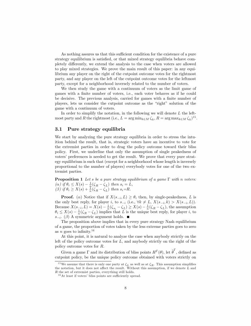
We start by analyzing the pure strategy equilibria in order to stress the intu-ition behind the result, that is, strategic voters have an incentive to vote forthe extremist parties in order to drag the policy outcome toward their blisspolicy. First, we underline that only the assumption of single peakedness ofvoters’ preferences is needed to get the result. We prove that every pure strat-egy equilibrium is such that (except for a neighborhood whose length is inverselyproportional to the number of players) everybody votes for one of the two ex-tremist parties.

Proposition 1 Let s be a pure strategy equilibrium of a game Γ with n voters:(α) if θi ≤ X(s)− 1

n(ζR − ζL) then si = L,(β) if θi ≥ X(s) + 1

n(ζR − ζL) then si=R.

Proof. (α) Notice that if X(s−i, L) ≥ θi then, by single-peakedness, L isthe only best reply, for player i, to s−i (i.e., ∀k 6= L, X(s−i, k) > X(s−i, L)).Because X(s−i, L) = X(s)− 1

n(ζsi − ζL) ≥ X(s)− 1n(ζR− ζL), the assumption

θi ≤ X(s)− 1n(ζR − ζL) implies that L is the unique best reply, for player i, to

s−i. (β) A symmetric argument holds.The proposition above implies that in every pure strategy Nash equilibrium

of a game, the proportion of votes taken by the less extreme parties goes to zeroas n goes to infinity.16

At this point, it is natural to analyze the case when anybody strictly on theleft of the policy outcome votes for L, and anybody strictly on the right of thepolicy outcome votes for R.

Given a game Γ and its distribution of bliss points HΓ(θ), let θ̃Γ, defined as

cutpoint policy, be the unique policy outcome obtained with voters strictly on15We assume that there is only one party at ζL as well as at ζR. This assumption simplifies

the notation, but it does not affect the result. Without this assumption, if we denote L andR the set of extremist parties, everything still holds.16At least if voters’ bliss points are sufficiently spread.

8

its left voting for L and voters strictly on its right voting for R, i.e., let θ̃Γbe

implicitly defined by:

θ̃Γ ∈ ζLH̄

Γ³θ̃Γ´+ ζR(1− H̄Γ

³θ̃Γ´)

where H̄Γ is the correspondence defined by H̄Γ(θ) =·limy→θ−

HΓ(y),HΓ(θ)

¸.

Let us assume that no player’s preferred policy coincides with the cutpointoutcome. No player on the left of the cutpoint outcome has an incentive tovote for any party different from L, because doing so would push the policyoutcome further away from his preferred policy. The same argument holds forany player on the right of the policy outcome. We can, then, state the followingproposition:

Proposition 2 If θi 6= θ̃Γ ∀i ∈ N , then the strategy combination given by

∀θi < θ̃Γsi = L and ∀θi > θ̃

Γsi = R is a pure strategy Nash equilibrium of the

game Γ.

It is clear that nothing assures us that pure strategy equilibria exist; more-over we have to check if mixed strategy equilibria prescribe a dramatically dif-ferent behavior for individual voters.

3.2 Mixed strategy equilibria

We analyze the case when players are allowed to play mixed strategies. In orderto undertake this analysis we have to assume also that the utility function u iscontinuously differentiable with respect to the first argument.17

We recall that, given the set of candidates M and the utility function u,a game Γ is characterized by the set of players and their bliss points. Let

σ = (σ1, ...,σn) and µ̄σ =Pi∈N

σin . With abuse of notation, letX(µ̄

σ) =mPk=1

ζkµ̄σk .

We can state the following proposition:

Proposition 3 ∀ε > 0, ∃n0 such that ∀n ≥ n0 if σ is a Nash equilibrium of agame Γ with n voters, then:(α) if θi ≤ X (µ̄σ)− ε then σi = L(β) if θj ≥ X (µ̄σ) + ε then σj = R.

Proof. See Appendix.In the appendix we will show that µ̄σ is the expected vote shares for the

parties. The proposition above says that in any Nash equilibrium, except for a17To study mixed strategies equilibria some cardinal assumptions on the utility function are

needed. Because we use the mean value theorem the cardinal assumption we have made isthe differentiability one, which seems to be the weakest one to get the results. Furthermore,the continuity of ∂u(X,θ)

∂Xin X guarantees the existence, for each player, of a lower bound on

the number of players for which the results hold. The continuity of ∂u(X,θ)∂X

in θ assures thata bound can be found independently of the set of players.

9

neighborhood whose length decreases as the number of players increases, every-body to the left of X (µ̄σ) votes for L, while everybody to the right votes forR.Using the definition of cutpoint policy outcome, we can state the main result

of this paper: essentially an unique Nash equilibrium of the game exists:

Corollary 4 ∀η > 0, ∃n1 such that ∀n ≥ n1 if σ is a Nash equilibrium of agame Γ with n voters, then:

(α) if θi ≤ θ̃Γ − η then σi = L

(β) if θj ≥ θ̃Γ+ η then σj = R.

Proof. Fix η and, in Proposition 3, take ε = η2 . For the corresponding n0

it is easy to see that if n ≥ n0 and σ is a Nash equilibrium of Γ, θ̃Γ − η

2 ≤X (µ̄σ) ≤ θ̃

Γ+ η

2 . In fact, suppose by contradiction that θ̃Γ − η

2 > X (µ̄σ) then

Proposition 3 implies that all voters to the right of θ̃Γvote for the rightmost

party and hence θ̃Γ ≤ X (µ̄σ), contradicting θ̃Γ − η

2 > X (µ̄σ). Analogously for

the second inequality. Hence θ̃Γ − η ≤ X (µ̄σ) − η

2 and θ̃Γ − η ≥ X (µ̄σ) + η

2 ,which, with Proposition 3, complete the proof.Every equilibrium conforms to such a cutpoint, and hence, for n large enough,

only the two extremist parties take a significant amount of votes.

3.3 Game with a continuum of voters

We now analyze analogous games with a continuum of voters. In such gamesevery strategy combination is a Nash equilibrium, because each player’s votedoes not affect the outcome. The results obtained in the previous pages leadus to analyze the game with a continuum of players as the limit game of gameswith a finite number of players. In such a case each voter behaves as if he couldbe decisive, and the “equilibrium” outcome is the policy obtained with everyvoter to its left voting for the leftmost party and every voter to its right for therightmost party.Let the bliss point distribution function characterizing the game with a con-

tinuum of voters H (θ) be continuous and strictly increasing, and let θ̃ be theunique policy outcome obtained with voters on the left of θ̃ voting for L andvoters on the right voting for R, i.e., θ̃ is the unique solution of

θ̃ = ζLH³θ̃´+ ζR(1−H

³θ̃´).

The previous analysis implies that θ̃ is the “equilibrium” of the game char-acterized by H(θ) when this game is seen as a limit of finite games.Moreover, considering the game with a continuum of voters, but where every

player acts as if his vote would be no-negligible, the cutpoint strategy can beobtained through a process of iterated elimination of dominated strategies, ifthe distribution function H(θ) is not too steep. This is the content of the nextproposition.

10

Proposition 5 Let H(θ) be differentiable. If

(ζR − ζL)H0(θ) < 1,

then θ̃ is the only strategy combination that survives the iterated elimination ofdominated strategies.

Proof. Given ζL, every player between 0 and ζL has voting for L as domi-nant strategy (whatever the others do, the outcome will be to his right). Hence,eliminating all the other strategies, every player between ζLH(ζL) + ζR(1 −H(ζL)) and 1 has voting for R as a dominant strategy. We can iterate thisprocess18. The iterations obey the following dynamic:

θt+1 = ζR − (ζR − ζL)H(θt)

which clearly converges to θ̃ if

(ζR − ζL)H0(θ) < 1.

4 Two ApplicationsWe have fully exploited the incentive for individual voters to vote for only twoparties when an election is called under proportional representation and thereare m parties. We want to apply our general result to two well-known modelsof political economy.

The first model we consider is Alesina and Rosenthal (1996). In such a modelthe policy outcome is described through a compromise between the executive,elected by plurality rule, and the legislature, elected by proportional rule. Con-sidering the two-stage game in which first the president and then the legislatureis elected, backward induction implies that in the second stage only the twoextremists will obtain votes. In the spirit of Alesina and Rosenthal’s analysis,we obtain a moderation result: we show that further right the president is, themore votes are taken by the leftmost party in the legislative election.We have pointed out in the introduction the empirical support for the mod-

eration result we obtain (Shugart 1995). Division of government (that is, whenmoderation shows its maximum effect giving the majority in the legislature tothe loser in the presidential election) is explained by Alesina and Rosenthal inthe following way: “division of power balances polarized parties” (1995:244).Clearly, in our model strategic voting explains this feature.

The second model we consider is that of Besley and Coate (1997), wherethe set of candidates is endogenous. Each citizen decides whether to become18The same conclusion can be obtained eliminating simultaneously the dominated strategies

of the leftist and the rightist voters (cf. the analogous procedure for a two-party model inIannantuoni (1999)). With such a procedure, however, we would have to analyze a system.For this reason we have preferred a simpler way to proceed.

11

a candidate, incurring a cost, or not. Our result implies that as the cost ofcandidacy goes to zero, only the two extremist citizens will be candidates.

We analyze both models assuming a continuum of voters and under theassumption that the distribution of bliss points H(θ) is strictly increasing andcontinuously differentiable, because in such a case we have uniqueness and differ-entiability of the “equilibrium”. We underline that the game with a continuumof voters has to be interpreted as an approximation of a finite game with a largenumber of voters.

4.1 Divided Government

In a recent paper, Alesina and Rosenthal (1996) describe the formation of na-tional policies as the result of institutional complexity that is captured by theexistence of two decision branches of the government: the executive (i.e., thepresident), elected under plurality rule, and the legislature, elected under pro-portional rule. In their model, two parties announce their policies and thenvoters vote. The main implication of this model is that “divided government”can be explained through the behavior of voters with intermediate (that is, sit-uated between parties’ announced positions) preferences, who take advantage ofthe institutional structure to balance the plurality of the winning party in theexecutive by voting for the opposite party in the legislative election. The mainresult of Alesina and Rosenthal can be expressed as: a party receives more votesin the legislative election if it has lost the executive election.In this section, we limit the analysis to a two-stage game in which first the

president and then the legislature is elected, and we show that analogous resultshold for any finite number of parties. More precisely, the results presented in theprevious section imply that, in the proportional stage, only the two extremiststake votes, and we show that the further to the right the president is, themore votes are taken by the leftmost party. As shown above, our solution restson purely individual behavior, viewing the game with a continuum of playersas a limit of finite games. Alesina and Rosenthal’s solution is instead basedon coalitions, to circumvent the difficulties arising from the fact that with acontinuum of voters everyone is negligible to the outcome.In the first stage players vote for the president, elected with plurality rule,

then in the second stage they vote for the legislature, elected with proportionalrule.Given the result of the elections, let the position of the legislature be given

by

X leg =mXk=1

ζkvk

where vk denotes the share of votes taken by party k, and let the policy outcomebe a convex combination of presidential and legislative positions:

X = (1− α)ζP + αXleg

12

where ζP denotes the position of the party winning the presidential election and0 < α < 1.Solving this game by backward induction, it is evident that, given the election

of the president P , the proportional stage is equivalent to the “proportionalgame” studied in the previous sections, with translated positions of the parties.In other words, given P , we have to analyze the “proportional game” with theset of parties MP where each party k is characterized by the policy

ζPk = (1− α)ζP + αζk.

The results of the previous sections imply that the equilibrium is such thatonly the two extremist parties19 L and R take votes. Moreover, the cutpoint

strategy θ̃Pis given by the unique solution to:

θ̃P= ζPLH(θ̃

P) + ζPR(1−H(θ̃

P),

which can be re-written as:

θ̃P= (1− α)ζP + αζR − α(ζR − ζL)H

³θ̃P´. (2)

Hence we have

∂θ̃P

∂ζP=

1− α

1 + αH 0³θ̃P´(ζR − ζL)

> 0. (3)

Because H(θ̃P) represents the share of votes taken in the legislative election

by the leftmost party and H(θ) is strictly increasing, (3) implies that such ashare is increasing in the position of the president. Hence also in multi-partysystems, we have a moderation result.The main difficulties in analyzing such a model arise in the presidential stage,

because multi-candidate election with plurality rule in a complete informationframework leads to a multiplicity of equilibria and, to have sensible solution, astrong refinement (as Mertens’ stability one) seems to be needed.20

Nevertheless, for some specification of the parameters of the model, theplurality stage can be solved by iterated elimination of dominated strategies.The following example shows a case where, given the equilibrium outcome foreach subgame, the plurality stage is dominance solvable and the center wins thepresidential election, while the two extremists win the legislative one.

EXAMPLE 2

There are three parties L,C, and R with ζL = 0, ζC =12 , and ζR =

35 . Sup-

pose the voters’ bliss points are distributed uniformly on [0, 1], with symmetricutility functions and α = 1

6 .

19Obviously we have L = argmink ζk = argmink ζPk and R = argmaxk ζk = argmaxk ζ

Pk .

20We refer to De Sinopoli (2000) for a discussion on this point.

13

If we solve the game backward, equation (2) gives us the equilibrium outcomefor each possible president. It is not difficult to compute that

θ̃L=1

11, θ̃C=31

66, and θ̃

R=6

11.

In the first stage, hence, citizens choose with plurality among θ̃L, θ̃C, and

θ̃R. Obviously we have the following preference orders on the election of L,C,

and R as president:

0 ≤ θi <37132 L Âi C Âi R

θi =37132 L =i C Âi R

37132 < θi <

722 C Âi L Âi R

θi =722 C Âi L =i R

722 < θi <

67132 C Âi R Âi L

θi =67132 C =i R Âi L

67132 < θi ≤ 1 R Âi C Âi LIn a plurality election, the strategy of voting for the least preferred candidate

is dominated (by voting for the most preferred). In the reduced game obtainedby eliminating such strategies, the players have the following strategies:

θi <722 L,C

θi =722 C

θi >722 R,C.

In this reduced game there is no chance of candidate L being elected presi-dent, because he takes at most 7

22 of the total number of votes. Hence votingfor him is dominated, as are voting for R if 7

22 < θi <67132 and voting for C if

67132 < θi ≤ 1. As a result, candidate C wins the plurality election, and in theproportional stage L and R take, respectively, 3166 and

3566 of the votes.

4.2 Representative Democracy

In this section we analyze what can happen when the set of candidates is notexogenous. To this end, we adopt a model analogous to Besley and Coate(1997). We consider a community consisting of a set of citizens N that, in orderto implement a policy X, must elect some representatives among themselves.The selection of the community representatives requires an election. Each

citizen is allowed to run for election, acting as a candidate. All citizens choosingto be a candidate face a utility cost δ.The political process consists of a three-stage game. In the first stage, each

citizen decides whether to become a candidate or not. In the second stage, theelection occurs. In the third stage, the policy is implemented. In Besley andCoate’s (1997) model the election is run with plurality rule and, because thereis no commitment, each elected candidate implements his preferred policy.

14

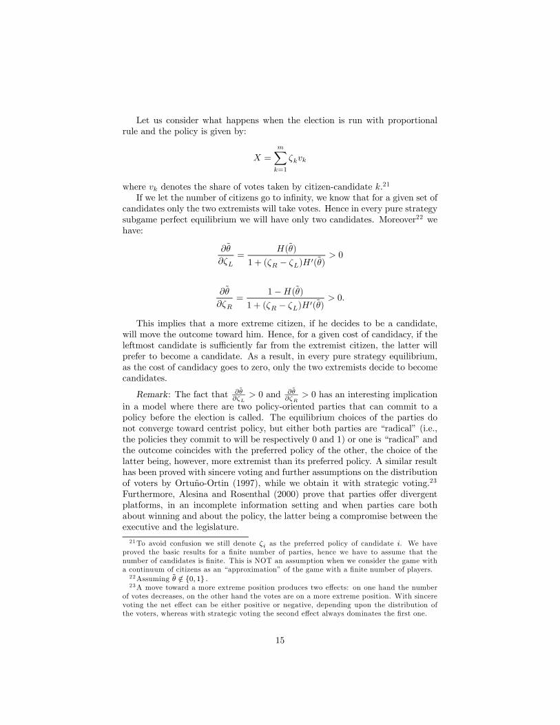
Let us consider what happens when the election is run with proportionalrule and the policy is given by:

X =mXk=1

ζkvk

where vk denotes the share of votes taken by citizen-candidate k.21

If we let the number of citizens go to infinity, we know that for a given set ofcandidates only the two extremists will take votes. Hence in every pure strategysubgame perfect equilibrium we will have only two candidates. Moreover22 wehave:

∂θ̃

∂ζL=

H(θ̃)

1 + (ζR − ζL)H0(θ̃)

> 0

∂θ̃

∂ζR=

1−H(θ̃)1 + (ζR − ζL)H

0(θ̃)> 0.

This implies that a more extreme citizen, if he decides to be a candidate,will move the outcome toward him. Hence, for a given cost of candidacy, if theleftmost candidate is sufficiently far from the extremist citizen, the latter willprefer to become a candidate. As a result, in every pure strategy equilibrium,as the cost of candidacy goes to zero, only the two extremists decide to becomecandidates.

Remark: The fact that ∂θ̃∂ζL

> 0 and ∂θ̃∂ζR

> 0 has an interesting implicationin a model where there are two policy-oriented parties that can commit to apolicy before the election is called. The equilibrium choices of the parties donot converge toward centrist policy, but either both parties are “radical” (i.e.,the policies they commit to will be respectively 0 and 1) or one is “radical” andthe outcome coincides with the preferred policy of the other, the choice of thelatter being, however, more extremist than its preferred policy. A similar resulthas been proved with sincere voting and further assumptions on the distributionof voters by Ortuño-Ortin (1997), while we obtain it with strategic voting.23

Furthermore, Alesina and Rosenthal (2000) prove that parties offer divergentplatforms, in an incomplete information setting and when parties care bothabout winning and about the policy, the latter being a compromise between theexecutive and the legislature.

21To avoid confusion we still denote ζi as the preferred policy of candidate i. We haveproved the basic results for a finite number of parties, hence we have to assume that thenumber of candidates is finite. This is NOT an assumption when we consider the game witha continuum of citizens as an “approximation” of the game with a finite number of players.22Assuming θ̃ /∈ {0, 1} .23A move toward a more extreme position produces two effects: on one hand the number

of votes decreases, on the other hand the votes are on a more extreme position. With sincerevoting the net effect can be either positive or negative, depending upon the distribution ofthe voters, whereas with strategic voting the second effect always dominates the first one.

15

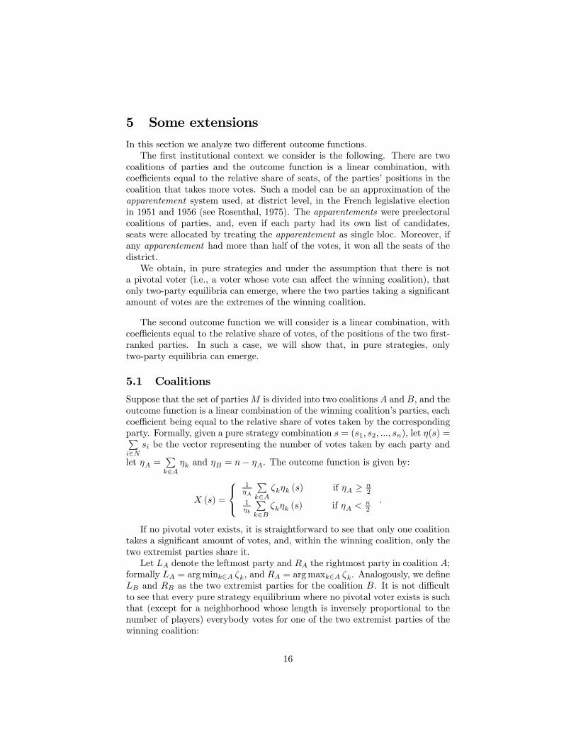
5 Some extensionsIn this section we analyze two different outcome functions.The first institutional context we consider is the following. There are two

coalitions of parties and the outcome function is a linear combination, withcoefficients equal to the relative share of seats, of the parties’ positions in thecoalition that takes more votes. Such a model can be an approximation of theapparentement system used, at district level, in the French legislative electionin 1951 and 1956 (see Rosenthal, 1975). The apparentements were preelectoralcoalitions of parties, and, even if each party had its own list of candidates,seats were allocated by treating the apparentement as single bloc. Moreover, ifany apparentement had more than half of the votes, it won all the seats of thedistrict.We obtain, in pure strategies and under the assumption that there is not

a pivotal voter (i.e., a voter whose vote can affect the winning coalition), thatonly two-party equilibria can emerge, where the two parties taking a significantamount of votes are the extremes of the winning coalition.

The second outcome function we will consider is a linear combination, withcoefficients equal to the relative share of votes, of the positions of the two first-ranked parties. In such a case, we will show that, in pure strategies, onlytwo-party equilibria can emerge.

5.1 Coalitions

Suppose that the set of partiesM is divided into two coalitions A and B, and theoutcome function is a linear combination of the winning coalition’s parties, eachcoefficient being equal to the relative share of votes taken by the correspondingparty. Formally, given a pure strategy combination s = (s1, s2, ..., sn), let η(s) =Pi∈N

si be the vector representing the number of votes taken by each party and

let ηA =Pk∈A

ηk and ηB = n− ηA. The outcome function is given by:

X (s) =

1ηA

Pk∈A

ζkηk (s) if ηA ≥ n2

1ηb

Pk∈B

ζkηk (s) if ηA <n2

.

If no pivotal voter exists, it is straightforward to see that only one coalitiontakes a significant amount of votes, and, within the winning coalition, only thetwo extremist parties share it.Let LA denote the leftmost party and RA the rightmost party in coalition A;

formally LA = argmink∈A ζk, and RA = argmaxk∈A ζk. Analogously, we defineLB and RB as the two extremist parties for the coalition B. It is not difficultto see that every pure strategy equilibrium where no pivotal voter exists is suchthat (except for a neighborhood whose length is inversely proportional to thenumber of players) everybody votes for one of the two extremist parties of thewinning coalition:

16

Proposition 6 Let s be a pure strategy equilibrium of a game with n voters,and assume that in s at least two parties in the winning coalition take somevotes.

(a) If ηA ≥ n+22 , θi ≤ X(s)− 2

n(ζRA − ζLA) implies si = LA and θi ≥ X(s) +2n(ζRA − ζLA) implies si = RA.

(b) If ηA <n−22 , θi ≤ X(s)− 2

n(ζRB − ζLB ) implies si = LB and θi ≥ X(s) +2n(ζRB − ζLB ) implies si = RB.

Proof. The conditions ηA ≥ n+22 and ηA <

n−22 imply that there is not a

pivotal voter. We show the first part of (a), the other cases being symmetric.Suppose si 6= LA. We have to analyze two cases:(i) si ∈ A\LA

X(s) > X (s−i, LA) = X (s)− 1ηA

¡ζsi − ζLA

¢> X(s)− 2

n(ζRA − ζLA) ≥ θiHence si ∈ A\LA cannot be a best reply to s−i(ii) si ∈ B

X(s) > X (s−i, LA) =ηA

ηA+1X (s)+ 1

ηA+1ζLA = X (s)− 1

ηA+1

£X (s)− ζLA

¤> θi

Hence si 6= LA is not a best reply.24

We stress that, in order to obtain the result, only the hypothesis on singlepeakedness of voters’ preferences is needed and an analogue to Proposition 2 canbe easily proved for each coalition. Moreover the result could be extended tomixed strategy equilibria, with the condition that, however, no player is pivotalamong the winning coalition, and to the case where there are more than twocoalitions.

EXAMPLE 3(a) There are 101 voters equidistant on the [0, 1] interval; i.e., one voter is

in 0, one voter is in 0.01 and so on until the last one, who is in 1. There aresix parties, positioned at {0, 0.2, 0.4, 0.6, 0.8, 1} and two coalitions, A and B.Coalition A is formed among the first three parties, and coalition B is formedamong the other three parties.It is easy to see that at least two equilibria conform to proposition 6.The first one, which leads to the victory of coalition A, is the following. Any

voter in [0, 0.28] votes for the leftmost party in coalition A, i.e., for the partysituated in 0; any voter in [0.29, 1] votes for the rightmost party in coalition A,i.e., for the party situated in 0.4. The resulting policy outcome is 288

1010 ' 0.285.Clearly any player in [0, 0.28] has no incentive to vote for any other party ofcoalition A or for any party of coalition B because by doing so, he would shiftthe policy outcome more to the right, i.e., further away from his bliss policypoint. At the same time any voter in [0.29, 1] has no incentive to vote for anyother party of the coalition, or for any party of coalition B, because by doingso, he would shift the policy outcome toward the left, i.e., further away from hisbliss policy.

24The condition that at least two parties in the winning coalition take some votes is necessaryto have, in this case, X(s) 6= X(s−i, LA).

17

The other equilibrium occurs when coalition B is the winning one, and anyvoter in [0, 0.71] votes for the leftmost party in the coalition, i.e. for the partypositioned in 0.6; while any voter in [0.72, 1] votes for the rightmost party inthe coalition, i.e., for the party positioned in 1, and the policy outcome is equalto¡721010.6 +

29101

¢ ' 0.714.(b) Let us consider an other case. Given the same set of voters and parties,

let coalition A be formed between parties located in 0 and in 1. Coalition B isformed among the other four parties.An equilibrium exists equilibrium such that any voter in [0, 0.49] votes for

coalition A and, within the coalition, for the party situated in 0; any voter in[0.51, 1] votes for coalition A and, within the coalition, for the party situated in1. The voter situated in 0.5 votes in such a way as not to affect the outcome,i.e., he casts his vote for any party in the losing coalition. The outcome resultingfrom the strategy combination above is 0.5, and it is simple to verify that thisis an equilibrium25.

5.2 Two Leading Parties

Up to now, we have analyzed the extreme situation in which the parties movethe outcome toward them with strength exactly proportional to the numbersof votes they take. At another extreme, we can consider a multi-party systemwhere only the two leading parties determine the political outcome. If theoutcome is a linear combination, with coefficients equal to the relative share ofseats, of the position of the two leading parties, we prove that, in pure strategies,only two-party equilibria can emerge.More formally, fix a strategy combination s. Define W 1 as the set of parties

that receive more votes under the strategy combination s. If this set containsonly one party, define W 2 as the set of parties that receives more votes, exceptW 1 (i.e., W 1 = {k : @k0s.t. vk0 > vk}, W 2 = {k : ∃!k0s.t. vk0 > vk}). If #W 1 ≥2, let I = argmink∈W1 ζk and II = argmaxk∈W 1 ζk. If #W

1 = 1, call I itselement and II the leftist element26 of W 2. In a multi-party system where theoutcome is a linear combination, with coefficients equal to the relative share ofseats, of the position of the two parties that take more votes27, we have:

X (s) =ζIvI + ζIIvIIvI + vII

(4)

In such a case we cannot obtain a “uniqueness” result as in section 3.Nevertheless, the following proposition implies that, in pure strategy equilib-ria, only two parties take a significant amount of votes. Given a pure strat-25Of course, other equilibria exist. For example, any voter in [0, 0.49] votes for coalition B,

and within the coalition for the party positioned in 0.2, and any voter in [0.51, 1] votes forcoalition B, and within the coalition for the party situated in 0.8, while the player in 0.50votes for any party in the losing coalition.26Or any other predefined element of W 2, as well as if #W 1 ≥ 3, we can choose the two

winning parties in any deterministic way. For our analysis it is necessary that every tie isdeterministically broken.27 If the ties are broken as we have done.

18

egy combination s, the set {I, II} of winning parties is deterministic. Letl (s) = argmink∈{I,II} ζk and r (s) = argmaxk∈{I,II} ζk. In the following, forsimplicity, we indicate l (s) as l and r (s) as r.

Proposition 7 Let the outcome function be as in (4), and let s be a pure strat-egy equilibrium of a game Γ with n voters. Then:(α) if θi ≤ X(s)− m(ζR−ζL)

2n then si = l

(β) if θi ≥ X(s) + m(ζR−ζL)2n then si = r.

Proof. (α) Suppose, by contradiction, that player i does not vote for partyl. Let nl (resp.nr) be the number of players who vote for l (resp. r), accordingto the pure strategy combination s. Clearly, nl + nr ≥ 2n

m . We distinguish thecase when player i votes for party r from the case when player i votes for anyother party.Suppose si = r. We have that:

X (s) > X(s) +1

nl + nr(ζl − ζr) = X(s−i, l) ≥ X(s)−

m(ζR − ζL)

2n≥ θi,

which contradicts s being an equilibrium.

Suppose si 6= r, hence X(s) > ζl. We have that:

X (s) > ( nl+nr

nl+nr+1)X(s) + 1

nl+nr+1θl = X(s)− 1

nl+nr+1(X(s)− ζl) =

= X(s−i, l) ≥ X(s)− 1nl+nr+1

(ζR − ζL) > θi,

which again contradicts s being an equilibrium.

(β) A symmetric argument holds.

Again, this proposition is based only on the single peakedness assumptionon voters’ preferences and an analogous of Proposition 2 can be easily provedfor each couple of parties. Also in this case the proof could be extended tomixed strategy equilibria, with the condition that, however, no player is pivotalamong the set of winning parties. Furthermore, we could get a two-party resulteven if the outcome function is a linear combination, with coefficients equalto the relative share of seats, of the positions of the m0 first ranked parties(2 ≤ m0 ≤ m). Unfortunately, we cannot analyze a mixed strategy equilibriumwithout the no-pivotal assumption, because a different behavior by a singleplayer could imply a dramatically different outcome. Hence our proof cannotbe extended for lack of continuity.

EXAMPLE 4Let’s take exactly the same set of parties and players as in example 3. It is

easy to see that the same argument developed for example 3 shows us that thestrategy combination where any voter in [0, 0.28] votes for the party situated in0 while any voter in [0.29, 1] votes for the party situated in 0.4 is an equilibrium,as is the strategy combination where any voter in [0, 0.71] votes for the partypositioned in 0.6 while any voter in [0.72, 1] votes for the party positioned in1. Moreover, the analogous argument of the case (b) in example 3 clarifies the

19

equilibrium represented by the strategy combination where any voter in [0, 0.49]votes for the party situated in 0, and any voter in [0.51, 1] votes for the partysituated in 1, while the player situated in 0.5 votes for any loser party in ordernot to affect the outcome.28

6 ConclusionThis paper is a first step in understanding the effect of strategic voting in pro-portional rule elections. The insight is quite “obvious”: under proportionalrepresentation strategic voters have an incentive to vote for the extremist par-ties in order to drag the policy outcome toward their ideal point. The mainconsequence is that Duverger’s hypothesis, that proportional representation fa-vors multi-partyism, may be incorrect under strategic voting. If the policy is aweighted average of parties’ platforms, with weights equal to the share of votes,or if the policy is the weighted average of the platforms of the members of thewinning preelectoral coalition, or if the policy is a weighted average of the toptwo vote-getters, only two parties get votes.

Future work will take into account many possible extensions that we onlybriefly cite here.Strategic parties. Readers familiar with spatial models of elections where

parties are the strategic players of the game may feel uncomfortable with theirabsence in this paper. For this reason, introducing parties as active players inthis game is the first extension we will undertake.Incomplete information. We assumed throughout the model that voters

possess complete information. In this respect, a natural extension is to considerchanges in this model when we add uncertainty.Multidimensional policy space. Another assumption that we think would be

interesting to relax is the unidimensionality of the policy space.Legislative bargaining. Finally, a very interesting research project is to un-

derstand how the policy outcome could be interpreted as a “reduced form” oflegislative bargaining.

It is clear that this paper represents a first step toward better understandingthe effect of strategic voting in proportional representation elections, and wehope that it will spur interest in this research agenda.

7 AppendixProof of proposition 3:(α) Given a mixed strategy σj , the player j’s vote is a random vector29

s̃j with Pr (s̃j = k) = σkj . Given σ−i = (σ1, ...σi−1,σi+1, ...σn), let−s̃−i=

28Of course other equilibria exist, for example, one for every possible pairs of parties.29We remind readers that a vote is a vector with m components.

20

1n−1

Pj∈N/i

s̃j and µ̄σ−i = 1n−1

Pj∈N/i

σj . The first step of the proof consists in

proving the following lemma:

Lemma 8 ∀φ > 0 and ∀δ > 0, if n > m4φ2δ

+ 1, then ∀σ,∀i

Pr

ï̄̄̄¯−s̃−i − µ̄σ−i

¯̄̄̄¯ ≤ ~φ

!> 1− δ.

Proof. To prove the lemma we can use Chebychev’s inequality componentby component. Given σ−i, it is easy to verify that E(s̃kj ) = σkj and V ar(s̃

kj ) =

σkj (1−σkj ) ≤ 14 , hence E(

−s̃−ik ) = µ̄

σ−ik and V ar(

−s̃−ik ) ≤ 1

4(n−1) . By Chebychev’sinequality we know that ∀k,∀φ:

Pr

ï̄̄̄¯−s̃−ik − µ̄σ−ik

¯̄̄̄¯ > φ

!≤ 1

4(n− 1)φ2 .

Hence

Pr

ï̄̄̄¯−s̃−i − µ̄σ−i

¯̄̄̄¯ ≤ ~φ

!≥ 1−

Xk

Pr

ï̄̄̄¯−s̃−ik − µ̄σ−ik

¯̄̄̄¯ > φ

!≥ 1− m

4(n− 1)φ2 ,

which is strictly greater than 1− δ for n > m4φ2δ

+ 1.

Now we show that ∀ε > 0, ∃n0 such that ∀n ≥ n0, if θi ≤ X (µ̄σ)− ε, thenL is the only best reply for player i to σ−i.Fix ε > 0. Define ∀θ ∈ £0, 1− ε

2

¤Mε (θ) = max

X∈[θ+ ε2 ,1]

∂u(X, θ)

∂X.

By single-peakedness we know that Mε (θ) < 0. Moreover, given the conti-nuity of ∂u(X,θ)

∂X we can apply the theorem of the maximum30 to deduce thatthe function Mε (θ) is continuous, hence it has a maximum on

£0, 1− ε

2

¤, which

is strictly negative. Let

M∗ε = maxθ∈[0,1− ε

2 ]Mε(θ).

LetM denote the upper bound31 of¯̄̄∂u(X,θ)∂X

¯̄̄on [0, 1]2, and let δ∗ε =

−M∗εM−M∗ε >

0 and φ∗ = (−2+√6)ε

m . We prove that if n > m4φ∗2δ∗ε

+ 1, then every strategy

30Because there are various versions of the theorem of the maximum, we prefer to stateexplicitly the version we are using (cf. Th.3.6 in Stokey and Lucas, 1989). Let f : Ψ×Φ→ <be a continuous function and g : Φ→ P (Ψ) be a compact-valued, continuous correspondence,then f∗(φ) := max {f(ψ,φ) | ψ ∈ g(φ)} is continuous on Φ.31The continuity of ∂u(X,θ)

∂Xassures that such a bound exists.

21

other than L cannot be a best reply for player i, which, setting n0 equal to thesmallest integer strictly greater than m

4φ∗2δ∗ε+ 1, directly implies the claim.

Take a party c 6= L. By definition c ∈ BRi (σ) =⇒Xs−i∈S−i

σ (s−i) [u (X (s−i, c) , θi)− u (X (s−i, L) , θi)] ≥ 0, (5)

which can be written as:Xs−i∈S−i

σ (s−i)·u (X (s−i, c) , θi)− u

µX (s−i, c)− 1

n(ζc − ζL), θi

¶¸≥ 0. (6)

Because the outcome function X (s) depends only upon v(s), denoting withV −in the set of all vectors representing the share of votes obtained by each partywith (n− 1) voters, (6) can be written as:X

v−in ∈V −in

Pr(−s̃−i= v−in )

·u¡X¡v−in , c

¢, θi¢− uµX ¡v−in , c¢− 1n(ζc − ζL), θi

¶¸≥ 0

(7)

where, with abuse of notation, X¡v−in , c

¢= ζc

n +n−1n

mPk=1

ζkv−in(k). Multiplying

both sides of (7) by nζc−ζL > 0 we have:X

v−in ∈V −in

Pr(−s̃−i= v−in )

£u¡X¡v−in , c

¢, θi¢− u ¡X ¡v−in , c¢− 1

n(ζc − ζL), θi¢¤

1n(ζc − ζL)

≥ 0.

(8)

By the mean value theorem we know that ∀v−in ,∃X∗ ∈ £X ¡v−in , c¢− 1

n(ζc − ζL),X¡v−in , c

¢¤such that£

u¡X¡v−in , c

¢, θi¢− u ¡X ¡v−in , c¢− 1

n(ζc − ζL), θi¢¤

1n(ζc − ζL)

=∂u(X, θi)

∂X

¯̄̄̄X=X∗

.

Hence we have:Xv−in ∈V −in

Pr(−s̃−i= v−in )

£u¡X¡v−in , c

¢, θi¢− u ¡X ¡v−in , c¢− 1

n(ζc − ζL), θi¢¤

1n(ζc − ζL)

≤

Pr(

¯̄̄̄¯−s̃−i − µ̄σ−i

¯̄̄̄¯ ≤ ~φ∗)M∗n(~φ∗, θi) + (1− Pr(

¯̄̄̄¯−s̃−i − µ̄σ−i

¯̄̄̄¯ ≤ ~φ∗))M

22

where

M∗n(~φ∗, θi) = max

X∈[X(µ̄σ−i−~φ∗,c)− 1n (ζc−ζL),1]

∂u(X, θi)

∂X.

Now we prove that, for n > m4φ∗2δ∗ε

+1, M∗n(~φ∗, θi) ≤M∗ε . From the definition

of M∗ε , it suffices to prove that M∗n(~φ∗, θi) ≤Mε(θi), which is true if X(µ̄σ−i −

~φ∗, c)− 1

n(ζc − ζL) is greater than θi +ε2 .

X(µ̄σ−i − ~φ∗, c)− 1n(ζc − ζL) =

n− 1n

Xk

µ̄σ−ik ζk −

n− 1n

Xk

φ∗ζk +1

nζL =

X(µ̄σ)− 1n

Xk

σki ζk +1

nζL −

n− 1n

Xk

φ∗ζk >

X(µ̄σ)− 1n(ζR − ζL)−mφ∗ζR ≥ θi + ε− 1

n−mφ∗.

Hence this step of the proof is concluded by noticing that δ∗ε is by definitionless than 1

2 , hence32

θi + ε− 1n−mφ∗ > θi + ε− 2φ

∗2

m−mφ∗ =

θi + ε− (20− 8√6)ε2

m3− ε

³−2 +

√6´≥ θi + ε(1− (20− 8

√6)

8+ 2−

√6) =

θi +1

2ε.

By Lemma 8, we know that, for n > m4φ∗2δ∗ε

+ 1,

Pr(

¯̄̄̄¯−s̃−i − µ̄σ−i

¯̄̄̄¯ ≤ ~φ∗)M∗n(~φ∗, θi) + (1− Pr(

¯̄̄̄¯−s̃−i − µ̄σ−i

¯̄̄̄¯ ≤ ~φ∗))M <

(1− δ∗ε)M∗ε + δ∗εM = (1− −M∗ε

M −M∗ε)M∗ε +

−M∗εM −M∗ε

M = 0.

32 In the following we assume that ε ≤ 1, since otherwise the proposition is trivially true.

23

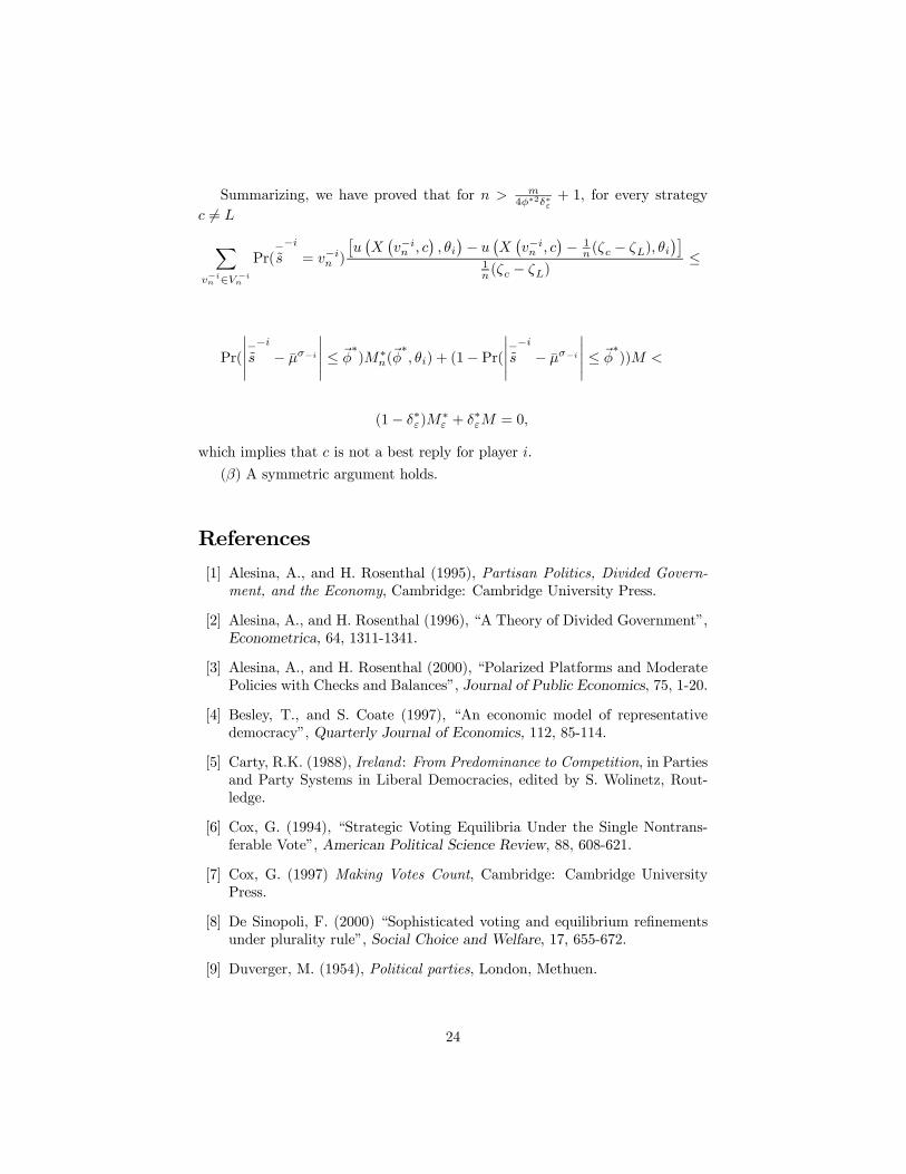
Summarizing, we have proved that for n > m4φ∗2δ∗ε

+ 1, for every strategyc 6= LX

v−in ∈V −in

Pr(−s̃−i= v−in )

£u¡X¡v−in , c

¢, θi¢− u ¡X ¡v−in , c¢− 1

n(ζc − ζL), θi¢¤

1n(ζc − ζL)

≤

Pr(

¯̄̄̄¯−s̃−i − µ̄σ−i

¯̄̄̄¯ ≤ ~φ∗)M∗n(~φ∗, θi) + (1− Pr(

¯̄̄̄¯−s̃−i − µ̄σ−i

¯̄̄̄¯ ≤ ~φ∗))M <

(1− δ∗ε)M∗ε + δ∗εM = 0,

which implies that c is not a best reply for player i.

(β) A symmetric argument holds.

References[1] Alesina, A., and H. Rosenthal (1995), Partisan Politics, Divided Govern-

ment, and the Economy, Cambridge: Cambridge University Press.

[2] Alesina, A., and H. Rosenthal (1996), “A Theory of Divided Government”,Econometrica, 64, 1311-1341.

[3] Alesina, A., and H. Rosenthal (2000), “Polarized Platforms and ModeratePolicies with Checks and Balances”, Journal of Public Economics, 75, 1-20.

[4] Besley, T., and S. Coate (1997), “An economic model of representativedemocracy”, Quarterly Journal of Economics, 112, 85-114.

[5] Carty, R.K. (1988), Ireland : From Predominance to Competition, in Partiesand Party Systems in Liberal Democracies, edited by S. Wolinetz, Rout-ledge.

[6] Cox, G. (1994), “Strategic Voting Equilibria Under the Single Nontrans-ferable Vote”, American Political Science Review, 88, 608-621.

[7] Cox, G. (1997) Making Votes Count, Cambridge: Cambridge UniversityPress.

[8] De Sinopoli, F. (2000) “Sophisticated voting and equilibrium refinementsunder plurality rule”, Social Choice and Welfare, 17, 655-672.

[9] Duverger, M. (1954), Political parties, London, Methuen.

24

[10] Engelmann, F. C. (1988), The Austrian Party System: Continuity andChange, in Parties and Party Systems in Liberal Democracies, edited by S.Wolinetz, Routledge.

[11] Fey, M. (1997) “Stability and Coordination in Duverger’s Law: A For-mal Model of Preelection Polls and Strategic Voting”, American PoliticalScience Review, 91, 135-147.

[12] Hotelling, H. (1929), “Stability in competition”, Economic Journal, 39,41-57.

[13] Iannantuoni, G. (1999), “Subgame perfection in a divided governmentmodel”, CORE DP.9928.

[14] Leys, C. (1959), “Models, Theories and the Theory of Political Parties”,Political Studies, 7, 127-146.

[15] Myerson, R. B., and R. J. Weber (1993), “A Theory of Voting Equilibria”,American Political Science Review, 87, 102-114.

[16] Ortuño-Ortin, I. (1997), “A spatial model of political competition and pro-portional representation”, Social Choice and Welfare, 14, 427-438.

[17] Palfrey, T. (1989), A mathematical proof of Duverger’s law. In: Ordeshook,P.C. (ed) Models of Strategic Choice in Politics, Ann Arbor, University ofMichigan Press.

[18] Riker, W.H. (1982), “The Two-party system and Duverger’s law: An essayon the history of political science”, American Political Science Review, 76,753-766.

[19] Rosenthal, H. (1975), “Viability, Preference, and Coalitions in the FrenchElection of 1951”, Public Choice, 21, 27-39.

[20] Sartori, G. (1968), Political Development and Political Engeineering, inPublic Choice, Cambridge: Cambridge University Press.

[21] Shugart, M. S. (1995), “The Electoral Cycle and Institutional Sources ofDivided Presidential Government”, American Political Science Review, 89,327-343.

[22] Stokey, N.L. and R.E. Lucas (1989), Recursive methods in economic dynam-ics, Cambridge, Massachusetts, and London, England, Harvard UniversityPress.

25