A Spatial Theory of Trade - Princeton Universityerossi/SToTAER.pdfA Spatial Theory of Trade By E...
28
A Spatial Theory of Trade By ESTEBAN ROSSI-HANSBERG* The equilibrium relationship between trade and the spatial distribution of economic activity is fundamental to the analysis of national and regional trade patterns, as well as to the effect of trade frictions. We study this relationship using a trade model with a continuum of regions, transport costs, and agglomeration effects caused by production externalities. We analyze the equilibrium specialization and trade pat- terns for different levels of transport costs and externality parameters. Understand- ing trade via the distribution of economic activity in space naturally rationalizes the evidence on border effects and the “gravity equation.” (JEL F1, R0, R3) Trade is spatial by nature. The distribution of economic activity in space determines the pat- tern of trade across and within countries. Con- versely, trade allows firms in a region to specialize in the production of a small number of goods, while consumers and firms demand a much larger basket of products. Casual obser- vation of the pattern of spatial specialization and employment concentration is enough to re- alize that the distribution of economic activity in space is not perfectly concentrated or uni- form. Hence, theories that imply a realistic dis- tribution of economic activity need to introduce the benefits and costs from spatial specializa- tion, namely, agglomeration and congestion forces. The benefits that firms in a particular location may derive from locating near firms in the same sector have to compensate for the extra costs of exporting production and importing intermediate inputs. This trade-off results in a variety of possible spatial patterns of production and trade flows that we study in this paper. The necessary agglomeration and congestion forces lead to a spatial trade theory that can ratio- nalize empirical observations that may seem hard to explain with standard trade arguments. One example is the effect of national borders on trade. The empirical literature has found that national borders reduce international trade flows and in- crease regional trade flows substantially. 1 What allows borders to have this important effect on trade flows and specialization patterns? Transport costs are ruled out, given that national borders matter even after controlling for distance. Other trade costs, like import taxes, would require either unreasonably high costs, or very high elasticities of trade with respect to these barriers. Clearly, high tariffs cannot account for the observed border effects of the European Union or North America. 2 What about a high elasticity of trade with respect to tariffs? The theory in this paper naturally de- livers this high elasticity. The idea is that tariffs imply a discontinuity in relative prices at borders, which changes specialization patterns. Agglomer- ation effects and transport costs amplify this effect in equilibrium—the first, since new or bigger clus- ters of firms affect the productivity of nearby firms, the second, since these new clusters supply goods mostly for the domestic market, conse- quently reducing international and increasing re- gional trade. 3 * Department of Economics and Woodrow Wilson School, Princeton University, Fisher Hall, Princeton, NJ 08544 (e-mail: [email protected]). I thank Robert E. Lucas, Jr., the editor Richard Rogerson, and a particularly helpful anonymous referee for many insightful comments. Fernando Alvarez, Rudiger Dornbusch, Liran Einav, Lars P. Hansen, Claudio Irigoyen, Boyan Jovanovic, Timothy Ke- hoe, Narayana Kocherlakota, Nancy Stokey, Mark Wright, Jaume Ventura, Kei-Mu Yi, and Mehmet Yorukoglu, as well as seminar participants at various institutions, provided helpful comments. 1 See John McCallum (1995), Shang-Jin Wei (1996), John F. Helliwell (1998), and James E. Anderson and Eric van Wincoop (2003). See also Holger C. Wolf (2000) and Thomas J. Holmes (1998) for the importance of state borders. 2 Notice, however, that such other barriers as different legal systems, languages, or currencies may have similar effects as deliberate trade policy. 3 See Daniel Trefler (2004) for evidence on effective U.S.-Canada trade tariffs. Helliwell (1998) and Charles Engel and John H. Rogers (1996) provide some evidence that border effects are important for relative prices. See 1464
Transcript of A Spatial Theory of Trade - Princeton Universityerossi/SToTAER.pdfA Spatial Theory of Trade By E...

A Spatial Theory of Trade
By ESTEBAN ROSSI-HANSBERG
The equilibrium relationship between trade and the spatial distribution of economicactivity is fundamental to the analysis of national and regional trade patterns aswell as to the effect of trade frictions We study this relationship using a trade modelwith a continuum of regions transport costs and agglomeration effects caused byproduction externalities We analyze the equilibrium specialization and trade pat-terns for different levels of transport costs and externality parameters Understand-ing trade via the distribution of economic activity in space naturally rationalizes theevidence on border effects and the ldquogravity equationrdquo (JEL F1 R0 R3)
Trade is spatial by nature The distribution ofeconomic activity in space determines the pat-tern of trade across and within countries Con-versely trade allows firms in a region tospecialize in the production of a small numberof goods while consumers and firms demand amuch larger basket of products Casual obser-vation of the pattern of spatial specializationand employment concentration is enough to re-alize that the distribution of economic activityin space is not perfectly concentrated or uni-form Hence theories that imply a realistic dis-tribution of economic activity need to introducethe benefits and costs from spatial specializa-tion namely agglomeration and congestionforces The benefits that firms in a particularlocation may derive from locating near firms inthe same sector have to compensate for the extracosts of exporting production and importingintermediate inputs This trade-off results in avariety of possible spatial patterns of productionand trade flows that we study in this paper
The necessary agglomeration and congestionforces lead to a spatial trade theory that can ratio-nalize empirical observations that may seem hardto explain with standard trade arguments One
example is the effect of national borders on tradeThe empirical literature has found that nationalborders reduce international trade flows and in-crease regional trade flows substantially1 Whatallows borders to have this important effect ontrade flows and specialization patterns Transportcosts are ruled out given that national bordersmatter even after controlling for distance Othertrade costs like import taxes would require eitherunreasonably high costs or very high elasticitiesof trade with respect to these barriers Clearlyhigh tariffs cannot account for the observed bordereffects of the European Union or North America2
What about a high elasticity of trade with respectto tariffs The theory in this paper naturally de-livers this high elasticity The idea is that tariffsimply a discontinuity in relative prices at borderswhich changes specialization patterns Agglomer-ation effects and transport costs amplify this effectin equilibriummdashthe first since new or bigger clus-ters of firms affect the productivity of nearbyfirms the second since these new clusters supplygoods mostly for the domestic market conse-quently reducing international and increasing re-gional trade3
Department of Economics and Woodrow WilsonSchool Princeton University Fisher Hall Princeton NJ08544 (e-mail erossiprincetonedu) I thank Robert ELucas Jr the editor Richard Rogerson and a particularlyhelpful anonymous referee for many insightful commentsFernando Alvarez Rudiger Dornbusch Liran Einav Lars PHansen Claudio Irigoyen Boyan Jovanovic Timothy Ke-hoe Narayana Kocherlakota Nancy Stokey Mark WrightJaume Ventura Kei-Mu Yi and Mehmet Yorukoglu aswell as seminar participants at various institutions providedhelpful comments
1 See John McCallum (1995) Shang-Jin Wei (1996)John F Helliwell (1998) and James E Anderson and Ericvan Wincoop (2003) See also Holger C Wolf (2000) andThomas J Holmes (1998) for the importance of stateborders
2 Notice however that such other barriers as differentlegal systems languages or currencies may have similareffects as deliberate trade policy
3 See Daniel Trefler (2004) for evidence on effectiveUS-Canada trade tariffs Helliwell (1998) and CharlesEngel and John H Rogers (1996) provide some evidencethat border effects are important for relative prices See
1464
Our theory provides a new angle to look atother related questions in trade Empirical stud-ies that use the gravity equation have shown thattrade flows decrease with distance a direct im-plication of the necessary congestion force4
Furthermore a spatial framework is necessaryfor transport costs and trade frictions to havedistinct effects on trade patterns and the volumeof trade5 Another immediate implication of aspatial setup is that relative prices of interme-diate goods are higher in countries that importthese goods as in the data6 More generally ourtheory can address questions on how trade bar-riers transport costs and technology affect thedistribution of economic activity in space andthe corresponding trade flows
The international trade literature has paid lit-tle attention to space Paul Krugman (1991b)pointed this out and presented a model of tradebetween two regions Following the publicationof his paper several studies have tried to modelspace and to demonstrate how space via trans-port costs can explain several puzzles in inter-national economics7 In virtually all papers inthis literature regions are modeled as points inspace land is not an input in production andfirms can locate only in one area or a smallnumber of areas within a country One note-worthy exception is Krugman and Venables(1995b) The paper presents a model of spatialspecialization between manufacturing and agri-cultural sectors with a continuum of locations Itassumes however that factors are geographi-cally immobile International barriers on migra-tion are important and we will consider thembut we relax the assumption of no regional orlocal mobility of labor Even more important
Krugman and Venables (1995b) do not studythe effect of trade frictions
Eaton and Kortum (2002) have written an-other paper in this tradition although with adiscrete number of locations They present aRicardian model of trade with geographic bar-riers which is successful in replicating the vol-ume and pattern of trade The paper assumesthat Total Factor Productivity (TFP) levels ineach industry are random realizations from adistribution with country-specific mean andcommon variance What determines the distri-bution of TFP Our view of trade implies thatthe agglomeration of firms in an industry at ageographic locationmdashthe pattern of geographicspecializationmdashis jointly determined in equilib-rium with the distribution of measured TFP
We build a spatial model of trade that con-siders a continuum of regions in a line To dothis we rely on two literatures the Ricardiantrade literature (as in Rudiger Dornbusch et al1977) and the urban literature (as in Robert ELucas Jr and Rossi-Hansberg 2002) Themodel can be seen as a spatial Ricardian modelof comparative advantage where technologicaldifferences are endogenous and determined byspatial specialization patterns through produc-tion externalities
The remainder of the paper is organized asfollows We set out the model in Section I anddiscuss the construction of an equilibrium inSection II In Section III we characterize theequilibrium and prove results related to themagnitude of relative prices across regions andthe effect of distance on trade flows Section IVintroduces trade barriers and discusses their ef-fect on trade flows Up to this point the paperassumes perfect labor mobility in Section V werelax this assumption and in Section VI wepresent several numerical simulations of themodel Section VII concludes
I The Model
The spatial structure is a line from S to Swhere S and S represent the northern andsouthern borders of the region under study Thesum of the length of all countries is 2S Thedensity of land at each point in the line is equalto one Throughout the paper we refer to alocation as a point in the line and to a region asan interval with positive length Countries areordered sequentially and are connected intervals
Kei-Mu Yi (2003 2005) for other theoretical explanations4 See for example Jeffrey H Bergstrand (1989) Marcos
Sanso et al (1993) Peter Egger (1999) and Simon JEvenett and Wolfgang Keller (1998)
5 This assumes that we set aside general equilibriumeffects resulting from the possible uses of tax revenue
6 See for example Jonathan Eaton and Samuel Kortum(2002) for empirical evidence
7 Some examples are Maurice Obstfeld and KennethRogoff (2000) Eaton and Kortum (2002) David Hummels(1999) Diego Puga and Anthony J Venables (1996 1997)Krugman and Venables (1995a) and Krugman (1991a1994 1995) Donald Davis and David Weinstein (2003)have shown empirically the presence and importance of thetype of home market effects that arise in spatial theories
1465VOL 95 NO 5 ROSSI-HANSBERG A SPATIAL THEORY OF TRADE
in the line For what follows in this section weassume that there are no restrictions to trade orto the flow of labor Hence for the moment thespecific location of borders is irrelevant In fol-lowing sections we analyze cases with thesetypes of restrictions
There are two goods a final good (FG) andan intermediate good (IG) Agents consume theFG only The FG is produced using land laborand the IG Production of the FG per unit ofland at some location r [S S] is given by
xFr gFzFrf FnFr cIr
where nF(r) is the number of workers per unit ofland specialized in the production of FGs at r(from now on the density of workers at r) cI(r)the demand for the IG per unit of land special-ized in the FG sector at r and zF(r) a productionexternality that depends on how many workersare employed at all locations in the FG sector
The IG is produced using land and laborProduction per unit of land of the IG at r isgiven by
xIr gIzIrf InIr
where nI(r) is the density of workers in thissector at r and zI(r) the sector-specific produc-tion externality Let i denote the elasticity of gi
with respect to zi i I FThe external effect in a sector depends on the
number of workers employed in the same sectorat each location It is supposed to be linear andto decay exponentially with distance at rate F
for the FG sector and I for the IG sector8
Hence in the FG sector
zFr S
S
FeFr snFss ds
where (r) is the proportion of land used for FGproduction at r So 1 (r) 0 for all r [S S] For the IG the external effect is cal-culated similarly
zIr S
S
IeIr snIs1 s ds
Agents consume only the FG they do notconsume land or the IG The utility of an agentliving and working at r is given by U(cF(r))where cF(r) denotes consumption of the FG at rThere is a perfectly elastic supply of workers atutility u so agents live and work at location r ifU(cF(r)) u That is there is free mobility oflabor across regions so the utility of eachworker is the same regardless of her locationThis implies that cF(r) cF U1(u) assum-ing that U is a strictly increasing function
It is costly to transport goods between loca-tions9 If one unit of good i is transported fromr to s only a fraction
eir s i F I
reaches s Namely we assume iceberg transportcosts where i is the transport cost per unit ofdistance in industry i We assume throughoutthe paper that i is positive and finite
Let pF(r) and pI(r) be the price of FGs andIGs respectively at r Then an agentrsquos wage atr must be given by wF(r) pF(r)cF and wF(r) wI(r) w(r) where the first equation is theagentrsquos budget constraint and the second resultsfrom free mobility across sectors Thus wagesare proportional to the price of FGs and realwages are constant at cF
Landlords are assumed to consume what theyearn from land rents at the location where theylive and they consume FGs only In FG re-gions landlords consume part of the produc-tion In IG regions landlords consume part ofthe imports of FGs Landlords do not work
The maximization problem of a firm thatproduces the IG at location r is given by
(1) maxn
pIrgIzIrf In wrn
8 Masahisa Fujita and Jacques-Francois Thisse (2002)show how this particular specification of external effectscan be justified as knowledge spillovers If the production ofideas requires the interaction between people working indifferent firms at different locations the closer other pro-ducers are the more ideas generated and hence the moreproductive firms in that region Guy Dumais et al (2002) JVernon Henderson (1988) Frank Pyke et al (1990) andAnnalee Saxenian (1994) provide evidence of this type ofexternalities at the regional level
9 See Hummels (1999) and Anderson and van Wincoop(2004) for empirical evidence on transport costs
1466 THE AMERICAN ECONOMIC REVIEW DECEMBER 2005
The first-order condition with respect to n is
pIrgIzIrf nII nIr wr pFrc F
Denote the relative price of IGs by p(r) pI(r)pF(r) then the first-order conditions define thedensity of workers in the IG sector (nI(p(r)zI(r)) nI(r)) as a function of the relative price ofthe IG and productivity zI(r)
The production of the IG at location r iscompetitive so firms take all prices as givenand earn zero profits Maximized output minuslabor costs (in units of FGs) is then the land bidrent of IGs firms (RI(r))
RIr prgIzIrf InIr c FnIr
Similarly the maximization problem of firmsin the FG sector at r is
(2)
maxnc
pFrgFzFrf Fn c wrn pIrc
So the first-order conditions are
gFzFrf nFnFr cIr c F
and
gFzFrf cFnFr cIr pr
These conditions define nF(p(r) zF(r)) nF(r)and cI(p(r) zF(r)) cI(r) as the density of work-ers in the FG sector and the demand of the IG asa function of the relative price of the IG andproductivity zI(r) Notice that the marginal productof labor in the FG sector is constant across loca-tions since real wages are constant Again the FGindustry is supposed to be competitive at all loca-tions and so firms earn zero profit The land bidrent of FG firms (RF(r)) is given by
RFr gFzFrf FnFr cIr
cFnFr prcIr
In order to impose equilibrium conditions inboth goods markets we need to keep track of thenumber of goods produced in each region theamount of goods traded and the number of goodslost in transportation Since the pattern of trade
across locations is endogenous and potentiallycomplicated it is difficult to define a standardequilibrium condition The following formulationallows us to impose equilibrium conditions in asimple way Let HF(r) be the excess supply of theFG accumulated between S and r once all therelevant trades in [S r] have been taken intoaccount and goods have been transported to loca-tion r Then by definition HF(S) 0 and inorder for the excess supply in the world to equalzeromdashequilibrium in the FG marketmdashwe needHF(S) 0 The evolution of this stock is dictatedby the following differential equation
HFr
r rxFr c FnF RFr
1 rcFnIr RIr
FHFr
At each location r we add to the stock of excesssupply the total production minus total consump-tion of the FG in the FG sector (r)[xF(r) cFnF RF(r)] and we subtract total consumptionof the FG in the IG sector (1 (r))[cFnI(r) RI(r)] We then need to take into account that ifHF(r) is positive as we increase r we need totransport FGs farther away from where they areproduced A fraction F of these goods is de-stroyed during transportation so we need to re-duce the accumulated excess supply accordinglyIf HF(r) is negative the intuition is similar
Using the definition of RF(r) and RI(r)mdashtheconsumerrsquos budget constraint and the firmrsquoszero profit conditionmdashwe can simplify theequation to get
(3)HFr
r
prrcIr 1 rxIr
FHFr
The construction of HI(r) parallels the one ofHF(r) so
(4)HIr
r 1 rxIr rcIr
IHIr
1467VOL 95 NO 5 ROSSI-HANSBERG A SPATIAL THEORY OF TRADE
At each location r we add the total productionof IGs (1 (r))xI(r) subtract the numberof IGs used for production in FGs sectors (r)cI(r) and adjust for extra transport costsIHI(r)
The balanced trade condition at each loca-tion r [S S] is then given by
(5) HFr prHIr 0
That is the sum of excess supplies expressed interms of FGs is zero at each location10 Theexpression takes into account goods consumedand produced at all locations but also the lossof some of these goods in transportation Animmediate implication is that for p(r) 0HF(r) 0 is equivalent to HI(r) 0 SoHF(S) 0 implies HI(S) 0 Walrasrsquos Law
Competition for land implies that land is as-signed to its highest value Namely
(6) RFr RIr implies r 1
(7) RFr RIr implies r 0 1 and
(8) RFr RIr implies r 0
Given zF and zI the Envelope Theorem impliesthat
RIr
pr gIzIrf InIr 0
and
RFr
pr cIr 0
for all r [S S] Define the mixed relativeprice pm as the relative price that equalizes thevalue of land in both sectors Given our assump-tions pm is well defined and unique The mixedrelative price pm(r) depends on r only throughthe productivity functions Hence (6) to (8) canbe restated as
(9) pr pm r implies r 1
(10) pr pm r implies r 0 1 and
(11) pr pm r implies r 0
So if for example the relative price of IGs at ris higher than a certain threshold pm(r) land ismore valuable if used in the production of IGs
In equilibrium agents buy goods from thelocation with the lowest price after transportcosts This implies that prices across locationshave to satisfy a no-arbitrage condition Sup-pose that a firm located at r is shipping IGs tolocation s Then by no arbitrage it has to be thecase that
pIr eIr spIs
Suppose that the condition is not satisfiedsince pI(r) eIr spI(s) Then IG firmsprefer to sell their goods at location r ratherthan at location s This however contradictsour original assumption that firms located at rwere shipping IGs to location s Suppose co-versely that pI(r) eIr spI(s) Thenagents could buy the good at location r trans-port it themselves and get the good at s atcost eIr spI(r) They could then sell thegood at location s making a profit an arbi-trage Hence the condition above has to besatisfied if IGs are being transported from r tos The same is true for FGs if FGs are beingtransported from r to s no arbitrage impliesthat
pFr eFr spFs
If goods produced at r are being shipped tolocation s HF(r) 0 for all r [r s]The reason is that if HF(r) 0 at somelocation r in between r and s after account-ing for all trades in region [S r] theexcess supply of the FG is zero This meansthat no goods are being traded between [Sr] and [r S] which contradicts the origi-nal assumption that r was trading with sHence we can divide the original interval[S S] into different regions with boundariesdefined by locations r where HF(r) 0 There istrade within these regions but no trade acrossthem
Balanced trade implies that if a region ex-ports IGs it has to import FGs If r exports IGs
10 The balanced trade condition can also be expressedonly in terms of local production and consumption asHF(r)r p(r)HI(r)r (I F)p(r)HI(r) 0
1468 THE AMERICAN ECONOMIC REVIEW DECEMBER 2005
to s s exports FGs to r11 This can happen viatrades with some locations in between r and sor directly Hence if the net flow of IGs from rto s is positive HF(r) 0 for all r [r s]
(12) pr eI Fr sps
If the net flow of FGs from r to s is positiveHF(r) 0 for all r [r s]
(13) pr eI Fr sps
If location r is a mixed areamdashan area whereboth goods are producedmdashit has to be the casethat no goods are shipped from or to location rThe reason is that if not prices would have tosatisfy (12) or (13) together with
pr pm r
This can happen but only at a point in space atransversal crossing Hence in mixed areasprices are given by pm and HF(r) HI(r) 0 so
1 rxIr rcIr
We still need to guarantee that it is not benefi-cial for other locations in the mixed area to buygoods from or sell goods to location r Sowhen (r) (0 1) prices have to satisfy
(14) eI Fr sps pr eI Fr sps
The condition guarantees that in mixed areasprices do not compensate for transport costsand so in equilibrium these areas do not trade
Let M be the space of nonnegative and con-tinuous functions For the definition of equilib-rium it is useful to define two operators T F M M3 M and T I M M3 M by
TFzF zIr
S
S
FeFr snFs zF zIs zF zI ds
and
TIzF zIr S
S
IeIr snIs zF zI
1 s zF zI ds
Notice that we are stressing in the notation thatnF nI and are functions of both productivityfunctions zF and zI In equilibrium the employ-ment densities that result from a pair of produc-tivity functions have to produce externalitiesthat result in the productivity levels implied bythese operators That is an equilibrium alloca-tion is a fixed point of these operators
We are ready to define an equilibrium in thiseconomy
DEFINITION An equilibrium is a set of func-tions nF nI cF cI zF zI HF HI p RI RF such that
(i) In all locations r [S S] U(cF(r)) u (ii) Firms solve problems (1) and (2)
(iii) Agents and firms buy goods from locationswith the lowest price after transport coststhe no-arbitrage conditions (12) (13) and(14) are satisfied
(iv) Land is assigned to its highest value soconditions (6) to (8) are satisfied
(v) HF and HI evolve according to equations(3) and (4)
HFS HIS HFS HIS 0
and for all r [S S] the trade balancecondition is satisfied
HFr pr HIr 0
(vi) For all r [S S]
TFzF zIr zFr and
TIzF zIr zIr
II Construction and Existence of anEquilibrium
The construction of an equilibrium in this setupfalls naturally into two steps The first step isto find an allocation that satisfies conditions (i)to (v) in the definition of equilibrium given the11 This implication holds only in a two-industry setup
1469VOL 95 NO 5 ROSSI-HANSBERG A SPATIAL THEORY OF TRADE
productivity functions (zF zI) The second step isto find a pair of functions (zF zI) such that con-dition (vi) is satisfied
Given a pair of productivity functions (zF zI)an allocation is uniquely determined by a relativeprice path p Let p(r ) be the relative price atlocation r associated with a price path starting at p(S ) At any location r as we increaser (move to the south) the relative price path has togrow at rate (F I) if HF(r) 0 decline at rate(F I) if HF(r) 0 either grow (if p(r) pm(r)) or decline (if p(r) 13 pm(r)) at rate (F I)or follow p(r) pm(r) if HF(r) 0 To constructan equilibrium relative price path we can startwith an initial relative price and follow theserules to obtain a candidate equilibrium relativeprice path Since every time HF(r) 0 and p(r) pm(r) the relative price path can evolve in threedifferent ways there may be many relative pricepaths associated with an initial relative priceHence each initial relative price path may beassociated with many final stocks of excess supplyof the FG
F HFS
That is F() is a correspondence We are look-ing for a such that 0 F() Numerically wecan do this using a shooting algorithm since HF(S) is decreasing in under the assumptions weimpose below We then need to find a fixed pointof the operators T F and T I which for i smallenough have iterates that converge
Proposition 1 guarantees that there existssuch a and an associated price path so that thefirst five equilibrium conditions are satisfiedProposition 2 uses Schauderrsquos fixed-point theo-rem to prove that there exists a pair of functions(zF zI) that satisfy condition (iv) Many of thearguments in the proofs of the theorems parallelthe arguments in Lucas and Rossi-Hansberg(2001) (the actual proofs can be found in Rossi-Hansberg 2003) The existence theorems areproven using the following assumptions
ASSUMPTION A
(i) Both gF and gI are continuously differen-tiable and concave
(ii) f F is continuously differentiable strictlyincreasing in both arguments strictly con-cave and f n
F (the marginal product of la-bor) is strictly increasing in cI
(iii) f I is continuously differentiable strictly in-creasing and strictly concave
(iv) There exists a pair of constants 0 13 such that for any x
gFx
and
gIx
(v) gF gI f F and f I satisfy for all cI
limx313
gFxf Fx cI
x lim
x313
gIxf Ix
x 0
(vi) U is strictly increasing and strictly con-cave
Part (iii) of Assumption A implies that whenthe relative price of IGs increases the density ofemployment in the FG sector decreases Part(iv) of Assumption A guarantees that the pro-ductivity of any firm is positive and that even ifthe external effect is infinitely large the produc-tivity of firms is bounded The magnitude ofthese bounds is arbitrary
PROPOSITION 1 Under Assumption A for anypair of positive and continuous productivity func-tions zF and zI there is an allocation that satisfiesconditions (i) to (v) Any such allocation is asso-ciated with a uniquely determined relative pricepath p(r) Except for intervals on which p(r) co-incides with the mixed path and with either (12) or(13) the allocation is uniquely determined
PROOFSee Rossi-Hansberg (2003)
PROPOSITION 2 Under Assumption A thereexists an equilibrium allocation That is thereexists a pair of functions (zF zI) such thatTF(zF zI)(r) zF(r) and T I(zF zI)(r) zI(r)
PROOFSee Rossi-Hansberg (2003)
The model can be seen as a Ricardian model ofcomparative advantage if we define equilibriumonly by conditions (i) to (v) given zI and zF In this
1470 THE AMERICAN ECONOMIC REVIEW DECEMBER 2005
case the productivity of each sector at each loca-tion is given exogenously and we can determinethe optimal distribution of production activitiesThis would be the case if for example naturalresources determine the productivity of regions inboth industries Once we add condition (vi) theequilibrium allocation cannot be proven to beunique This implies that the initial productivityfunctionsmdashused as a starting point in the algo-rithm to construct an equilibriummdashdetermine theequilibrium that is reached One interpretation ofthis dependence is that history matters Locationof firms in different sectors and their productivityat some point in time determine the equilibriumallocation in the future
The potential multiplicity of equilibria in thissetup is limited by the presence of the endpointsS and S Since there is no production beyondthese points locations at these boundaries tendto have lower productivity We could insteadthink about the distribution of economic activityin a circle where these endpoint effects are notpresent In a circular world we need to analyzeequilibria up to a rotation given the lack ofgeography If spillovers decline fast enoughwith distance so the effect of the endpoints onproductivity is small the role of endpoints isalmost entirely to select one allocation out ofthe continuum of identical equilibria in the cir-cular world One can show numerically that thisis the case for the examples in Section VI Notethat in a world without endpoints as in thecircular spatial setup it is impossible to thinkabout countries that are isolated because of theirgeography The United States and Argentinawould have the same spatial characteristics In aworld with geography and therefore with end-points as in our setup we can think about thelocation of countries in the world
III Characterization of an Equilibrium
In order for an allocation to be an equilib-rium prices have to satisfy the no-arbitrageconditions and land has to be assigned to itshighest value From these two properties we canconstruct a graph that is helpful in understand-ing how land is assigned to its different usesGiven the productivity functions we can calcu-late pm for all locations Equations (9) to (11)imply that if the relative price of IGs is abovepm the region produces IGs so 0 If therelative price is below pm the area produces
FGs 1 and if it is equal it produces bothgoods (0 1) We also know from (12) to(14) that as r increases the relative price func-tion has to grow at rate (F I) (F I)or be equal to pm Given a relative price at Swe can construct a relative price function usingthe rules above Proposition 1 guarantees thatthere is a unique relative price at S that satis-fies the goods market equilibrium conditions(v) At locations where HF(r) HI(r) 0 thereis a kink in the relative price function Thereason is that shipments of goods change direc-tion at 0 The construction is illustrated in Fig-ure 1 if we focus on the curves marked p and pmonly At S p(S) pm(S) so the regionclose to the left boundary sells IGs and the pricefunction grows with r When p crosses pm weswitch to an FG-producing region At r 0HF(0) 0 and so the flow of goods changesdirection which implies a kink in the pricefunction that now decreases with r
In this construction relative prices of IGs arehigher in FG-producing regions than in adjacentIG-producing regions This confirms our claimthat the model is consistent with high capitalgoods prices in developing countries Relativeprices of IGs may be low or high in regions thatproduce both goods We formalize the result in thefollowing proposition the proof is included in theAppendix
PROPOSITION 3 The relative price of IGs ishigher in regions such that 1 than inadjacent regions such that 0
Since prices adjust according to transport costsfirms in a particular location are indifferent abouttrading with several partners That is prices adjustto compensate for transport costs in regions suchthat HF does not change sign (FGs are beingshipped in one direction only) If HF(r) 0 thereis no trade between locations r r and locationsr r We need a definition of bilateral trade thatis consistent with this characteristic of the modelIf goods are being shipped between two locationswe can think about all locations in between themas importing the shipment adding their own ex-ports or taking out their imports and shipping theremaining goods further We can then define tradebetween two locations as the minimum (becauseof trade balance) of the flow of goods that passesthrough each of them Formally define trade be-tween two locations r and s where r s as
1471VOL 95 NO 5 ROSSI-HANSBERG A SPATIAL THEORY OF TRADE
Trr s minHF(r) HF(s)if HF(r) 0 r (r s)
0 otherwise
With this definition at hand we can show thatdistance reduces bilateral trade
PROPOSITION 4 If two locations producedifferent goods the closer they are the morethey trade
An equilibrium in this economy exhibitsother properties that are worth mentioning
The equilibrium allocation depends only onthe sum of transport costs F I it isevident that only the sum matters in the con-struction of the equilibrium price path Usingtrade balance it is easy to write the equilib-
rium conditions as a function of the sum oftransport costs only
Given the productivity functions highertransport costs imply more regions in au-tarky higher transport costs increase the ab-solute value of the slope of the price functionwhich then crosses the mixed relative pricecurve more often
As transport costs go to infinity all loca-tions are in autarky and prices and produc-tion are determined only by productivityfunctions
As transport costs go to zero the price func-tion is constant and at least one good is pro-duced in only one region
As the land share in production goes to zeroin one sector the sector concentrates in oneregion and the size of the region decreaseswith
FIGURE 1 THE EFFECT OF AN IMPORT TAX WITH FIXED PRODUCTIVITIES
1472 THE AMERICAN ECONOMIC REVIEW DECEMBER 2005
IV Trade Barriers
Thus far we have described a world withoutfrictions in which agents and firms are freelymobile and so national borders do not play arole In this section we give countries the pos-sibility to levy taxes on the imports and exportsof goods and analyze the equilibrium implica-tions of trade policy Assume that a country thatexports FGs decides to impose a tax on theimports of IGs from a particular country Sup-pose for example that this country occupieslocations [s2 s3] and that the country fromwhich it imports IGs occupies locations [s1 s2]Then the relative price of IGs has to satisfy
pr eI Fr sps
for r (s2 s3] and s [s1 s2) where is thetax per unit of the IG Other types of tariffs canbe introduced in an analogous way The resultof such a policy is that the country that exportsFGs produces more IGs and the other countryproduces more FGs This is a spatial version ofthe standard effect of tariffs In contrast withstandard theories however this setup allows usto analyze what happens with prices and thelocation of production activity within bothcountries when the tax is imposed
Figure 1 illustrates the example given pro-ductivity functions Country 2 specializing inFGs imposes a tax on the imports from Country1 The solid line is the relative price of IGswithout taxes Once the tax is imposed therelative price of IGs in Country 2 goes up at theborder This is illustrated by the solid thin linein the figure The tax prompts some locations inCountry 2 to switch and produce the IG insteadof the FG This allocation cannot be an equilib-rium since at these prices the world producestoo many IGs There is an excess supply of IGswhich leads to a decrease in the relative price ofIGs at all locations The resulting relative priceis the dashed line Notice that because of thedecrease in the price of IGs some locations inCountry 1 start producing FGs
This example stresses two implications of themodel First transport costs and trade barriershave very different effects on the equilibriumallocation Without trade barriers the relativeprice function is continuous Different transportcosts imply a different evolution of the relativeprice function but no discontinuities If instead
of having a continuum of regions we had con-sidered several points in space (as most of theprevious literature) we could not make thisdistinction so by assumption as Obstfeld andRogoff (2000) point out the model would implythat tariffs and transport costs have exactly thesame effect Second trade barriers reduce tradeas expected and increase the set of goods thateach country produces Once we allow the pro-ductivity function to adjust these effects ontrade flows are even larger Producing the FG inCountry 1 makes this country better at produc-ing FGs Trade policy affects the productivity atwhich different goods are produced by chang-ing the distribution of economic activity inspace
In the next Proposition we formalize theeffect of trade barriers given productivity func-tions Tariffs reduce international trade and in-crease regional trademdashthe spatial version of thestandard effect of tariffs Proofs of the next twopropositions appear in the Appendix
PROPOSITION 5 Given a pair of productivityfunctions trade frictions at the border that aresmall enough not to imply trade reversalsweakly reduce trade between countries andweakly increase trade within countries
If productivity is allowed to adjust this effectis amplified creating a larger border effect Thestandard implication in Proposition 5 is ampli-fied in equilibrium thereby increasing the elas-ticity of trade with respect to tariffs We canformalize the result under some conditions Thefirst one is that production externalities decreasefast enough with distance The restriction isnecessary since we want the local increase inproduction of the protected good to influencelocal productivity more than the decrease inproduction in other countries Given that mostexamples of regional externalitiesmdashlike SiliconValley or Route 128mdashinvolve relatively smallregions we do not believe that this is a veryrestrictive assumption
We also need no trade reversals The reason isthat countries may start exporting a different goodafter imposing the tariff and they potentiallycould export large amounts This however doesnot imply that the elasticity of trade barriers issmall since with trade reversals the effective tar-iff or friction becomes zero The last condition isnecessary because of the potential multiplicity of
1473VOL 95 NO 5 ROSSI-HANSBERG A SPATIAL THEORY OF TRADE
equilibria in the model Starting from an equilib-rium without tariffs we need to determine whichof the potentially many equilibria we reach Prop-osition 6 presents the result
PROPOSITION 6 (Amplification effect) Inequilibrium trade frictions at the border weaklyreduce trade between countries and weakly in-crease trade within countries The effects arelarger than the effects given productivity func-tions if
Production externalities decrease fastenough with distance (high F and I)
Trade frictions at the border are smallenough not to imply trade reversals and
F and I are small enough so that startingfrom an equilibrium with productivity func-tions (zF zI) the sequence of functions(T
F)n(zF zI) and (TI)n(zF zI) n 1 2
converge The operators TF and T
I are de-fined for the economy with frictions
The last condition is a condition on F and IIf i 0 so the price function does not react atall to changes in (zF zI) we are in the case ofProposition 1 and the operator converges in onestep If i is very large increases in zi substan-tially increase productivity at different loca-tions which in turn implies large changes inland use patterns Large changes in land usepatterns may imply that the iterative procedureto find an equilibrium which is the basis of theproof may not converge For small enough i the iterations always converge these are thecases for which the proposition applies
V Restrictions on International Labor Mobility
Probably the specification of the model closerto reality is to allow for labor mobility inside acountry but not across countries Migration lawsrestrict mobility of workers in almost all nationsin the world (Europe is an example for whichthe version presented so far is better suited) Inthis subsection we modify the setup to allowworkers to move freely inside a country but notacross countries Free mobility of labor equal-izes the utility of agents in a country Hence inthis version of the model utility levels varybetween but not within countries In order toincorporate the no-migration restriction we canproceed in two ways We can define the utility
levels of agents in each country and let thepopulation size be determined in equilibrium orwe can determine the population size in eachcountry and let the utility levels be determinedin equilibrium
For the first case we need to specify a utilitylevel for each country Let the number of coun-tries be given by an integer NC and the twoborders of each country be given by B (i) andB (i) for i 1 2 NC where B (i) B (i 1) by definition Denote the utility level ofagents in country i by u(i) i 1 2 NCThen condition (i) in the definition of equilib-rium becomes
(i) For all r [B (i) B (i)) i 1 NC
UcFr u i and UcFS u NC
The rest of the analysis follows as in previoussections Notice that the modified definition ofequilibrium implies that for U strictly increas-ing cF(r) is a step function with constant valueinside each country and different value betweencountries That is real wages vary between butnot within countries
For the second case we need to determine thepopulation of each country exogenously LetPop(i) be the population size in country i Then
(15) Popi B i
Bi
rnFr
1 rnIr dr i 1 NC
is the equilibrium condition in country irsquos labormarket In this case the utility of agents in countryi u(i) is determined in equilibrium Condition (i)in the definition of equilibrium then becomes
(i) For all r [B (i) B (i)) i 1 NC
UcFr u i and UcFS u NC
Population sizes in all countries are given by(15)
Again all other features of the model pre-sented in previous sections remain unchangedThe two cases presented above (exogenous util-ities or population sizes) are equivalent That isthere is a one-to-one mapping between coun-
1474 THE AMERICAN ECONOMIC REVIEW DECEMBER 2005
trysrsquo population sizes and utility levels12 SincecF is not a continuous function nF nI cI xFand xI may not be continuous functions eitherHence pm has discontinuities at national bor-ders Nevertheless the relative price function isstill continuous in the absence of trade barriers
VI Numerical Examples
In this section we illustrate the differentequilibrium possibilities of the model with nu-merical examples In all examples we use aCobb-Douglas specification for the utility func-tion and both production functions so
xFr zFrFnFrF
cIrF
xIr zIrInIrI
and
UcFr cFr
The basic parameterization used is given byF I 009 F 08 F 01 I 07 08 F I 5 and F I 0005These parameter values constitute the bench-mark case from which we illustrate several pos-sible equilibrium allocations13 All the resultspresented in the next subsection are for the caseof perfect labor mobility using u 1 In orderto construct an equilibrium we also need tostart the algorithm with an initial pair of pro-ductivity functions (zF zI) This choice willselect one of the potentially multiple equilib-rium allocations of our model To compute thebenchmark case we use a uniform distributionfor both sectors All other examples are com-puted using the pair of equilibrium distributions
of the benchmark case as the initial productivitydistributions In all the computed examples theequilibrium allocation has IG regions at the twoboundaries This characteristic of the examplespresented is the result of our choice of initialdistributions Other initial distribution will leadto equilibria with FG regions at the edges
Figure 2 presents the benchmark case Thetop panel presents the price and mixed rela-tive price functions as well as land rents(divided by two for visibility) The bottompanel presents the excess supply functions inboth sectors As described above there is aregion at the center producing the FG and therest of the world produces the IG The IGregion on the left trades with the closest halfof the FG region (the region to the left of thekink in the relative price curve) There is notrade between this IG region and the otherhalf of the FG region relative prices do notcover transport costs so producers prefer totrade with regions that are closer It is evidentthat regions trade with the closest region thatproduces the good they do not produce andthat relative prices of IGs are higher in FG-producing regions than in IG areas Landrents decline as we approach the boundariesS and S or the boundaries between regionsthat produce different goods given the lack ofexternalities from firms in the other sector orthe absence of firms Note that this decline ishowever modest at the boundaries S and Swhich implies that the role played by theendpoints in the equilibrium allocation is rel-atively small The concentration of economicactivity in the FG region implies high produc-tivity and in most locations higher land rentsthan in the IG sector This is the result of thelarger labor share in the FG production func-tion and of spillovers that depend on the num-ber of workers employed in the same sector insurrounding locations14
A Transport Costs
Transport cost parameters are of particular im-portance for the qualitative features of the equi-librium If transport costs are very high locationsdo not trade and the solution of the model is
12 To see this remember that the first-order conditionswith respect to employment densities of the firmsrsquo problemsare given by gF(zF(r)) fn
F(n(r) (r) cI(r)) U1(u(i)) andp(r)gI(zI(r)) fnI
I (nI(r)) U1(u(i)) where r [B (i) B (i))Hence under Assumption A a higher utility level in coun-try i implies a lower employment density in both industriesOf course changes in the utility function will change theproductivity and prices at different locations and so theproof is more complex
13 Notice that in order for part (iv) of Assumption Ato be satisfied we need to use the following specificationxF(r) min[ zF(r)F
]nF(r)FcI(r)F
and xI(r) min[ zF(r)F
]nI(r)I However we can choose low
enough and high enough so that the bounds do not play a rolein the results The parameter values chosen are such that all theother parts of Assumption A are satisfied
14 Since land rents always follow prices and productivityin the same way we omit them in all other graphs
1475VOL 95 NO 5 ROSSI-HANSBERG A SPATIAL THEORY OF TRADE
FIGURE 2 EQUILIBRIUM ALLOCATION FOR F I 0005
1476 THE AMERICAN ECONOMIC REVIEW DECEMBER 2005
autarchy at all locations Since locations near theboundaries S and S are on average farther awayfrom other locations employment densities arelower near these boundaries
If transport costs are low regions specializecompletely This is the case for the FG sector inthe example presented in Figure 2 for F I 0005 Higher transport costs (F I 01)imply two distinct FG regions as shown in Fig-ure 3 In this example there are four regions inwhich there is trade within the region but notrade between regions These areas can be iden-tified as the areas between the kinks in therelative price curve These kinks correspond tothe locations at which both HF and HI are equalto zero Trade flows are much lower than in theprevious case as is the level of economic ac-tivity and TFP given the smaller productionclusters Population declines by 74 percent rel-ative to the benchmark case Hence highertransport costs not only reduce trade but alsoeliminate trade between certain regions com-pletely The intuition for these results is simpleas transport costs increase the gains from con-centrating production of the FG become smallerthan the costs of shipping FGs and IGs longdistances This increases the bid rent of IG firmsat the center of the FG cluster in Figure 2 whichbecomes higher than the bid rent of FG firmsand so a new IG region appears
B Externality Parameters
There are two parameters that govern theeffect of production externalities on the dis-tribution of economic activity and trade Thefirst parameter i i F I determines theextent to which spillovers affect output Inparticular it determines the elasticity of pro-duction with respect to zi A parameter i
close to one implies that productivity reactsalmost one to one to changes in zi So in thiscase an increase in zi affects productivity bythe same amount no matter the level of zi Forzi close to zero the effect of changes in zi ismuch larger for firms that experience smallspillover effects than for firms that experiencelarge spillover effects Figure 4 illustrates theeffect of changes in i on the excess supplyfunctions HF and HI The solid line is thebenchmark case with F I 009 and welet F 075 As we decrease F to 008 theFG region expands and the IG regions at the
boundary become smaller A lower F impliesthat there are fewer incentives to agglomerateeconomic activity in the FG sector since thebenefits of higher spillovers decrease whichexpands the FG region A decrease in F alsoimplies that the average spillover declinesand so there is a general level effect thatdecreases the level of economic activity in allFG areas This decrease affects IG producerssince their good is used as an input only in theproduction of FGs Total population de-creases by 427 percent when F 008 andby 646 percent when I 008 relative tothe benchmark case A decrease in I gener-ates the opposite effect IG areas expand andFG regions contract As before we obtain ageneral negative effect on the level of eco-nomic activity
Hence if an industry is in its first stages ofinnovation where spillovers are likely to belarge the industry is geographically concen-trated As these spillovers become less impor-tant we see more regions producing in thatindustry and lower productivity This is remi-niscent of what has happened in certain indus-tries for example the computer industry Firmsstarted in very concentrated areas and as theirproduct became more standard they moved toless expensive cities and regions
The second parameter governing externalitiesis i i F I A high i implies that spilloversdecline faster with distance but the averagelevel of spillovers remains constant Numericalexercises for different values of i are presentedin the lower panel of Figure 4 As i increaseseconomic activity concentrates in sector i Outputdeclines more sharply at the boundaries of theregions producing the good with higher i Incontrast with the upper panel in this case there isno level effect on output Population declines onlyby 52 percent relative to the benchmark casewhen F 10 and by 107 percent when F 1The smaller is F the less dispersed is productionwithin the FG region For example as communi-cation technology becomes better spillovers de-cline more slowly with distance Some sectorstherefore tend to expand and are less concentratedin a few clusters
This seems consistent with the expansion ofglobal manufacturing In the twentieth centurymanufacturing moved away from a couple ofproduction centers in developed countries tomany locations around the world
1477VOL 95 NO 5 ROSSI-HANSBERG A SPATIAL THEORY OF TRADE
FIGURE 3 EQUILIBRIUM ALLOCATION FOR F I 01
1478 THE AMERICAN ECONOMIC REVIEW DECEMBER 2005
FIGURE 4 EQUILIBRIUM TRADE PATTERN FOR DIFFERENT EXTERNALITY PARAMETERS (F 075)
1479VOL 95 NO 5 ROSSI-HANSBERG A SPATIAL THEORY OF TRADE
C Labor Shares
Labor shares i i F I are also animportant determinant of the distribution ofeconomic activity As the labor share of aparticular industry increases since the overalltechnology exhibits constant returns to scaleland shares decrease Hence increases in la-bor shares are always reductions in landshares Figure 5 presents excess supply func-tions HF and HI for different labor shares inFG production In all cases labor shares inthe IG sector are constant at 07 The solidline in the top panel represents the excesssupply functions associated with the sameexercise presented in Figure 2 FG productionis very concentrated at the center Laborshares are large and so production of FGsuses relatively small amounts of land As wedecrease the labor share FG production be-comes more land intensive and so FG areasexpand In the top panel we keep fixed theutility of agents and therefore real wages soemployment in the economy can vary As wedecrease labor shares employment decreasessubstantially since labor is less important inproduction and real wages are fixed Thesechanges are larger and in the same directionas we lower the labor share further Howeverthe decrease in employment as we go fromF 08 to 075 is much larger (896 per-cent) than the decline (346 percent) as we gofrom 075 to 070 The reason is that in thefirst case the FG sector becomes more inten-sive in land than in IGs As a sector becomesmore labor intensive production concentratesin a few clusters The large population declineimplies a decline in the level of economicactivity
In order to control for the effect on popula-tion we calculate another set of exercises wherepopulation sizes are fixed and we vary utilitylevels This eliminates the scale effect in the toppanel and reverses the implication on concen-tration As capital shares in the FG sector de-crease labor becomes relatively less expensivethan land and firms in the sector concentratemore Real wages decrease as we make theFG technology less labor intensive (u 105100 and 089 for F 08 075 and 07respectively)
The exercise suggests that industries in whichnew workers can enter easily (eg low human
capital) should be more concentrated the highertheir labor shares On the contrary industrieswhere entry of new workers is costly (eg highhuman capital requirements) should be less con-centrated the larger their labor shares
D Taxes and Border Effects
In previous sections we have argued that thetheory generates amplified border effects Weillustrate this result using as a benchmark theequilibrium presented in Figure 2 Divide theworld into three countries where the first andthird countries produce only the IG and thesecond only the FG The equilibrium in Figure2 then implies that the border between Coun-tries 1 and 2 is at 132 and the border betweenCountries 2 and 3 is at 132 Let Country 2impose a 40-percent tax on the imports of Coun-try 1rsquos IGs The resulting allocation given zF
and zI is presented in Figure 6 With importtaxes a new region in Country 1 produces FGsand a new region in Country 2 produces IGsNevertheless Country 1 still exports IGs andimports FGs from Country 2
The simulation presented in Figure 6 takes asgiven a pair of productivity functions The func-tions are the equilibrium productivities for F I 0005 Once we adjust the productivityfunctions we obtain the equilibrium presentedin Figure 7 Once agglomeration effects aretaken into account the tariff completely elimi-nates trade between Countries 1 and 2 Country1 is in autarchy The left side of the countryproduces the IG and the right side the FGBecause there is no trade between Country 1and other countries relative prices do not haveto jump 40 percent at the border The disconti-nuity is just large enough to guarantee that thereis no excess supply of any of the goods inCountries 2 and 3 Country 2 produces bothgoods the IG near its borders and the FG in themiddle Country 3 imports FGs from Country 2and exports IGs Trade flows between Countries2 and 3 increase with respect to the originalequilibrium with F I 0005 This is whyas Anderson and Wincoop (2003) argue it isimportant to control for average tariffs in esti-mations of the Gravity equation The increase inthe pm function in Country 1 shows how firmsoperating near the border become more produc-tive in the FG sector The production external-ity together with transport costs amplifies the
1480 THE AMERICAN ECONOMIC REVIEW DECEMBER 2005
FIGURE 5 EQUILIBRIUM TRADE PATTERN FOR DIFFERENT LABOR SHARES
1481VOL 95 NO 5 ROSSI-HANSBERG A SPATIAL THEORY OF TRADE
FIGURE 6 EQUILIBRIUM WITH IMPORT TAX AND FIXED PRODUCTIVITIES
1482 THE AMERICAN ECONOMIC REVIEW DECEMBER 2005
FIGURE 7 EQUILIBRIUM WITH IMPORT TAX
1483VOL 95 NO 5 ROSSI-HANSBERG A SPATIAL THEORY OF TRADE
effect of the tariff to the extent that it com-pletely eliminates trade between Countries 1and 2 Regions in Country 1 trade more betweenthemselvesmdashbecause they are closer and thereare transport costsmdashand Country 1 does nottrade with the rest of the world This is themechanism that creates important border effectsin the model It implies a larger-than-standardelasticity of trade with respect to barriers
E Taxes and Border Effects withoutInternational Labor Mobility
As we described in Section V we can set upthe model restricting international labor mobil-ity The conclusions from the example shown inFigure 7 also hold in this case Let the popula-tion sizes in each country be given by the ex-ercise presented in Figure 2 Population inCountries 1 and 3 is small and equal and pop-ulation in Country 2 is substantially larger Weimpose the tax and calculate the new equilib-rium holding population sizes in each countryfixed The results look very similar to the resultsin the case with international migration Coun-try 1 is in autarky Again we obtain a highelasticity of trade with respect to tariffs higherthan what standard models would predict
An important difference between the exam-ple with international labor mobility and thisone is that the current one gives us predictionson the utility levels of workers Workers inCountry 2mdashthe one that imposes the taxmdashendup losing from the policy the other two coun-tries gain Utility of workers in all previousexamples is equal to 1 In this case utility ofworkers is 1035 in Country 1 0974 in Country2 and 109 in Country 3 The average utility ofworkers in the world decreases to 099 Hencethe world as a whole is better off with free tradebut individual countries may gain from impos-ing tariffs this can only be the case with mi-gration restrictions Note that the countries thatgain do not have to be the countries that imposethe tariffs Since the FG is more intensive inlabor than the IG (more intensive in land) asCountry 2 substitutes production of FGs forIGs it employs fewer people Thus wages haveto decrease to eliminate the excess supply oflabor This is the main cause for the decline inutility Conversely the opposite effect is themain reason for the increase in worker utility inCountry 1
F Trade Policy and Multiple Equilibria
In our theory temporary trade policy can havepermanent effects Suppose Country 1 occupiesthe interval [5 05] and Country 2 the interval[05 5] Let F I 002 The equilibrium inthis case implies that Country 1 exports IGs toCountry 2 Suppose Country 2 imposes a tax of 20percent on the imports of IGs from Country 1 Inthe new equilibrium with perfect labor mobilityand tariffs both countries are in autarky Whathappens if we now remove the tariff NothingThe new equilibrium without tariffs is identical tothe equilibrium with barriers The reason is thatproductivities change in such a way that countrieswould not trade even if it were costless Figure8 presents the original equilibrium the equilib-rium given productivities and the new equilib-rium with and without taxes Autarky is not theonly way this can happen trade reversals areanother possibility Country 1 may become soproductive at producing FGs that it may startexporting them In this case the tariff on IGs is noteffective and so reducing or removing it has noeffect Permanent effects of trade policy as theone illustrated above suggest a potential explana-tion for why in some cases trade liberalizationhas not led to large increases in trade flows Thereare however examples in which removing orreducing the tariff does change the equilibriumallocation In fact this is the case in the equilib-rium presented in Figure 7
VII Conclusion
We have presented a theory of the spatialdistribution of economic activity and the asso-ciated trade patterns On the methodology sidethe model presented uses a constant returns-to-scale technology with production externalitiesThis helps us model firmsrsquo location and land usedecisions with a continuum of regions whichhas the advantage of allowing for a very richvariety of concentration and specialization pat-terns in a model that is suitable for both analyt-ical and computational study This setup hasallowed us to talk about changes in fundamen-tals as well as trade policy without loosing theability to derive conclusions for both within-and between-country trade This flexibilitycomes at a cost namely that the productionexternality is a black boxmdasha reduced form rep-resentation of the interactions between firms
1484 THE AMERICAN ECONOMIC REVIEW DECEMBER 2005
Understanding trade through the concentra-tion and specialization patterns in space pro-vides a novel rationalization of several tradefacts In our framework the distribution of eco-nomic activity depends on the size of transportcosts and externality parameters and these fun-damentals determine intra-national and interna-tional flows of goods Our analysis emphasizesthat including space as we have done differen-tiates clearly the role of transport costs andtariffs The change in specialization created byborder frictions is amplified by the agglomera-tion effects transport costs and the spatialstructure resulting in an amplification of fric-tions at national bordersmdasha higher than stan-dard elasticity of trade with respect to barriersThis conclusion is not affected by assump-tions on international labor mobility The mag-
nitude of the amplification is directly related tothe magnitude of agglomeration forces Wehope this paper stimulates empirical studies ofthe link between border and agglomerationeffects
The model is consistent with estimations ofthe gravity equation both within and acrosscountries Results on the gravity equation forregions inside the European Union and forstates in the United States may corroborate thisconclusion The implication that equipmentprices are higher in developing countries than indeveloped economies is a natural outcome ofhaving a continuum of regions and transportcosts Hence although the model does deliverthe result it would be interesting to see if thedifferences in relative prices are of a magnitudeconsistent with transport costs
FIGURE 8 TRADE POLICY AND MULTIPLE EQUILIBRIA
1485VOL 95 NO 5 ROSSI-HANSBERG A SPATIAL THEORY OF TRADE
Our setup can be used to understand a widerange of regions and policies In particular onecould start with other initial productivity func-tions that yield different spatial configurationsAs pointed out in Section II since the equilib-rium of the model may not be unique the initialproduction structure in a region or group ofcountries may determine the equilibrium andso history matters Furthermore the paper high-lights how temporary trade policy can select aparticular equilibrium allocation In this sensethe history of trade policy matters for the cur-rent allocation This may rationalize cases inwhich trade liberalization has had disappointingeffects
A possible extension of the theory is to study
the evolution of concentration and specializa-tion patterns as economies develop15 Themodel has predictions on the link between thesemeasures transport costs and productivitygrowth but as it stands it is static Anotherextension is to add several consumption goodsThis may help explain clusters in a variety ofindustries and the associated patterns of con-sumption with the potential to understand theldquohome-bias in consumption puzzlerdquo These ex-tensions are left for future research
APPENDIX PROOFS OF PROPOSITIONS 3 4 5 AND 6
PROOF OF PROPOSITION 3The proposition can be restated as If HF(s) 0 for all s [r r] r r (r) 0 and (r)
1 then p(r) p(r) If HF(s) 0 for all s [r r] r r (r) 1 and (r) 0 then p(r) p(r) The proof is an immediate consequence of the no-arbitrage conditions (12) and (13) Take thecase where HF(s) 0 for all s [r r] r r (r) 0 and (r) 1 then condition (12) impliesthat p(r) e(FI)rrp(r) which yields the result for F I 0
If HF(s) 0 for all s [r r] r r (r) 1 and (r) 0 then condition (13) implies thatp(r) e(FI)rrp(r) and so p(r) p(r)
PROOF OF PROPOSITION 4The proposition can be restated as If r s r s and (r) (s) (r) (s) 1 then
Tr(r s) 13 Tr(r s)If r s r s and (r) (s) (r) (s) 1 then Tr(r s) 13 Tr(r s) Let s be such
that for all r (r s) HF(r) 0 Then if HF(s) 0 HF(s)r 0 and if HF(s) 0 HF(s)r 0 Hence Tr(r s) 13 Tr(r s)
Let s be such that there exists an r (r s) such that HF(r) 0 Then Tr(r s) 0 and Tr(rs) 0 The second part of the proof for r and r is analogous
PROOF OF PROPOSITION 5Let the intervals [B1 B2] and [B3 B4] represent Country 1 and 2 respectively where B2 13
B3 Without loss of generality assume that Country 1 is exporting the IG to Country 2 (so bycurrent account balance Country 2 exports the FG to Country 1) Define trade between Country1 and 2 by
TrsB TrB2 B3 minHF(B2) HF(B3) if HF(r) 0 r (B2 B3)
0 otherwise
Let (S11 S2
1 ) be a sequence of numbers such thatS1
1 B1
15 See Sukkoo Kim (1995) Jean M Imbs and RomainWacziarg (2003) and Karl Aiginger and Stephen W Davies(2004) for empirical evidence
1486 THE AMERICAN ECONOMIC REVIEW DECEMBER 2005
S21 minarg max
s B1
Hs B2
Si1 min arg max
s Si 11
Hs B2
and define n1 by n1 minn Sn1 B2 We can build a sequence of numbers (S1
2 S22 Sn2
2 ) in a parallelway where S1
2 B3 Then trade within Country j 1 2 can be defined by
TrsW j
i 1
nj 1
maxr S i
jS i 1j
HFreFBj 1r maxHFS1j eFBj 1S 1
j HFSn jj eFBj 1S nj
j
We need to show that the presence of a trade friction reduces TrsB and increases Trs
W(j) j 1 2Given the assumed flow of trade again without loss of generality assume that Country 2
imposes a trade tariff on the imports of IGs from Country 1 (any effective friction at the bordermay be reduced to this example) Then p(r) decreases for r [B1 B2] and p(r) increases forr [B3 B4] as illustrated in Figure 1 This implies under Assumption A that xF(r) decreasesweakly for r [B3 B4] and so since transport costs have not changed that HF(B2) decreasesweakly (see Lemma 1 in Rossi-Hansberg 2003) Country 1 is exporting IGs so HF(B2) 0 Adecrease in p(r) for r [B1 B2] implies that xF(r) increases weakly for r [B1 B2] and soHF(B2) 0 increases weakly or HF(B2) weakly decreases Hence the trade friction implies areduction in Trs
BTo show that Trs
W(1) increases first notice that the expression
maxHFS1j eFBj 1S 1
j HFSn jj eFBj 1S nj
j
takes the values HF(B1)eFB2B1 and HF(B2) for j 1 Notice also that
maxr B1 S 2
j
HFreFB2 r HFB1eFB2B1 0
and
maxr S n1
j B2
HFreFB2 r HFB2 0
We have proven above that HF(B2) weakly decreases Since p(r) decreases for r [B1 B2] and thisimplies that xI(r) decreases weakly and xF(r) increases weakly for r [B1 B2]
i 2
n12
maxr Si
1Si 11
HFreFB2r
increases weakly Locations with r B1 also experiences a decrease in the price of IGs As a resultHF(B1) increases weakly However by definition the increase in
maxr B1 S2
j
HFreFB2 r
has to be equal or larger Hence TrsW(1) increases weakly Exactly the same logic applies for Country
2 Hence TrsW(1) and Trs
W(2) increase weakly
1487VOL 95 NO 5 ROSSI-HANSBERG A SPATIAL THEORY OF TRADE
PROOF OF PROPOSITION 6First note that the tax creates the same effects described in Proposition 5 plus it changes productivities
Let p(r) be the relative price of an equilibrium without trade frictions and let p(r) be the relative priceof the short-term equilibrium (given productivity functions) with trade frictions Without loss ofgenerality assume that Country 1 [B1 B2] exports the IG to Country 2 [B3 B4] where B2 B3 Asdiscussed above the frictions create a discontinuity in p so that p(r) p(r) for r [B1 B2] and p(r) p(r) for r [B3 B4] This implies that
B1
B2
1 r dr 13 B1
B2
1 r dr
and
B3
B4
r dr 13 B3
B4
r dr
where (r) is the fraction of land use to produce FGs at location r in the ldquoshort-termrdquo equilibriumwith frictions (given productivity function) That is a smaller or equal amount of land is specializedin the production of the IG in Country 1 and a smaller or equal amount of land is specialized in theproduction of the FG in Country 2 This implies that a larger or equal proportion of land is used forthe production of the FG in Country 1 and a larger or equal proportion of land is used for theproduction of the IG in Country 2 By Assumption A (see Lemma 1 in Rossi-Hansberg 2003)p(r) p(r) implies that x
I(r) xI(r) and xF(r) xF(r) for r [B1 B2] and so Assumption A (ii)
and (iii) imply that nI(r) nI(r) and n
F(r) nF(r) for r [B1 B2] Similarly for Country 2 p(r) p(r)implies that x
I(r) xI(r) and xF(r) xF(r) for r [B3 B4] and so Assumption A (ii) and (iii) imply that
nI(r) nI(r) and n
F(r) nF(r) for r [B1 B2] Hence there exists a F and a I such that
TFzF zIr zFr r B1 B2
TIzF zIr zIr r B1 B2
and
TFzF zIr zFr r B3 B4
TIzF zIr zIr r B3 B4
The high pair of (F I) is needed so that the lower spillover coming from the reduction ofemployment in the FG industry in Country 2 for example does not dominate the higher spillovercoming from the increase in production of FGs in Country 2 The level of spillovers is not importantthe rate of decline with distance is
We need to show that the change in productivities described above holds for further iterations that isif we keep applying the operators T
F and TI we get monotone effects on productivity of final and IG
production We also need to show that these changes in productivity lead to less international trade andmore regional trade To show that the effects on productivity of further iterations are monotone for someF and a I notice that higher zF(r) in Country 1 for example weakly increases (r) and nF(r) for r [B1 B2] This by Lemma 1 in Rossi-Hansberg (2003) increases the relative price of IGs in Countries1 and 2 which in turn increases the production of IGs in both countries Hence the effect in productivityhas to weakly dominate the effect in relative prices in Country 1 So Country 1 employs a larger or equalnumber of workers in the FG sector which implies that for F high enough (ie this effect dominates theeffect of fewer FG workers in Country 2)
TF2zF zIr T
FzF zIr zFr r B1 B2
1488 THE AMERICAN ECONOMIC REVIEW DECEMBER 2005
The same argument applies for all other changes in productivity in both countries Hence there exista F and a I such that changes in productivity are monotone in each iteration
We now turn to show that this increase in productivity implies a further reduction in tradeflows between countries and a further increase in trade within nations Clearly the first iterationimplies the effects in Trs
B and TrsW(i) i 1 2 that we analyzed in Proposition 5 If we can show
that the increases in productivity described above also imply a reduction in TrnB and an increase
in TrnW(i) i 1 2 (where the subscript n denotes that this is the nth iteration of the operators)
then we have proved the existence of the amplification effect if the successive application of theoperators T
F and TI converges For this notice that a lower productivity of Country 2 in the
production of FGs implies that Country 2 produces fewer FGs this implies by Lemma 1 alower relative price of IG but as discussed above the effect in productivity dominates so thefinal result is fewer exports of FGs from Country 2 Hence HF(B3) and HF(B2) fall since weare assuming no trade reversals Therefore
TreB TrB2 B3
decreases Since the change in the productivities is monotone if the sequence of iterations con-verges the reduction in Tre
B is larger than the reduction in TrsB because of the adjustment in
productivitiesTo show that regional trade increases notice that the change in productivities implies that
for example Country 1 is producing more FGs and fewer IGs (the effect in productivitiesweakly dominates the effect in price) Since the country is still exporting the IG (no tradereversals) this implies that regional trade has to increase This implies that as in the proof forProposition 5
i 2
n12
maxr Si
1Si 11
HFreFB2 r
increases and the other terms weakly increase by construction Therefore the increase in produc-tivities increases Tre
W(i) i 1 2 Hence if the sequence of iterations converges the equilibriumeffect on regional trade is larger than the ldquoshort-termrdquo effect
REFERENCES
Aiginger Karl and Davies Stephen W ldquoIndus-trial Specialization and Geographic Con-centration Two Sides of the Same CoinNot for the European Unionrdquo Journal ofApplied Economics 2004 7(0) pp 231ndash48
Anderson James E and van Wincoop EricldquoGravity with Gravitas A Solution to theBorder Puzzlerdquo American Economic Review2003 93(1) pp 170ndash92
Anderson James E and van Wincoop EricldquoTrade Costsrdquo Journal of Economic Litera-ture 2004 42(3) pp 691ndash751
Bergstrand Jeffrey H ldquoThe Generalized GravityEquation Monopolistic Competition and theFactor-Proportions Theory in InternationalTraderdquo Review of Economics and Statistics1989 71(1) pp 143ndash53
Davis Donald R and Weinstein David E ldquoMar-ket Access Economic Geography and Com-parative Advantage An Empirical TestrdquoJournal of International Economics 200359(1) pp 1ndash23
Dornbusch Rudiger Fischer Stanley and Sam-uelson Paul A ldquoComparative Advan-tage Trade and Payments in a RicardianModel with a Continuum of Goodsrdquo Amer-ican Economic Review 1977 67(5) pp823ndash39
Dumais Guy Ellison Glenn and GlaeserEdward L ldquoGeographic Concentrationas a Dynamic Processrdquo Review of Eco-nomics and Statistics 2002 84(2) pp193ndash204
Eaton Jonathan and Kortum Samuel ldquoTrade inCapital Goodsrdquo European Economic Review2001 45(7) pp 1195ndash235
Eaton Jonathan and Kortum Samuel ldquoTechnol-
1489VOL 95 NO 5 ROSSI-HANSBERG A SPATIAL THEORY OF TRADE
ogy Geography and Traderdquo Econometrica2002 70(5) pp 1741ndash79
Egger Peter ldquoA Note on the Proper Econo-metric Specification of the Gravity Equa-tionrdquo Economics Letters 2000 66(1) pp25ndash31
Engel Charles and Rogers John H ldquoHow WideIs the Borderrdquo American Economic Review1996 86(5) pp 1112ndash25
Evenett Simon J and Keller Wolfgang ldquoOnTheories Explaining the Success of the Grav-ity Equationrdquo Journal of Political Economy2002 110(2) pp 281ndash316
Fujita Masahisa and Thisse Jacques-FrancoisEconomics of agglomeration Cities in-dustrial location and regional growthCambridge Cambridge University Press2002
Helliwell John F How much do national bor-ders matter Washington DC Brookings In-stitution Press 1998
Henderson J Vernon Urban development The-ory fact and illusion Oxford Oxford Uni-versity Press 1988
Holmes Thomas J ldquoThe Effect of State Policieson the Location of Manufacturing Evidencefrom State Bordersrdquo Journal of PoliticalEconomy 1998 106(4) pp 667ndash705
Hummels David ldquoToward a Geography ofTrade Costsrdquo Purdue University Center forGlobal Trade Analysis (GTAP) Working Pa-per No 17 1999
Imbs Jean and Wacziarg Romain ldquoStages ofDiversificationrdquo American Economic Re-view 2003 93(1) pp 63ndash86
Kim Sukkoo ldquoExpansion of Markets and theGeographic Distribution of Economic Activ-ities The Trends in US Regional Manufac-turing Structure 1860ndash1987rdquo QuarterlyJournal of Economics 1995 110(4) pp881ndash908
Krugman Paul R Geography and trade Cam-bridge MA MIT Press 1991a
Krugman Paul R ldquoIncreasing Returns and Eco-nomic Geographyrdquo Journal of PoliticalEconomy 1991b 99(3) pp 483ndash99
Krugman Paul R ldquoComplex Landscapes inEconomic Geographyrdquo American EconomicReview 1994 (Papers and Proceedings)84(2) pp 412ndash16
Krugman Paul R Development geography andeconomic theory Cambridge MA MITPress 1995
Krugman Paul R and Venables Anthony JldquoGlobalization and the Inequality of Na-tionsrdquo Quarterly Journal of Economics1995a 110(4) pp 857ndash80
Krugman Paul R and Venables Anthony J ldquoTheSeamless World A Spatial Model of Interna-tional Specializationrdquo National Bureau ofEconomic Research Inc NBER WorkingPapers No 5220 1995b
Lucas Robert E Jr and Rossi-HansbergEsteban ldquoOn the Internal Structure of Cit-iesrdquo Econometrica 2002 70(4) pp 1445ndash76
McCallum John ldquoNational Borders MatterCanadandashUS Regional Trade PatternsrdquoAmerican Economic Review 1995 85(3) pp615ndash23
Obstfeld Maurice and Rogoff Kenneth ldquoThe SixMajor Puzzles in International Macroeco-nomics Is There a Common Causerdquo in BenS Bernanke and Kenneth Rogoff edsNBER macroeconomics annual 2000 Cam-bridge MA MIT Press 2001
Puga Diego and Venables Anthony J ldquoTheSpread of Industry Spatial Agglomeration inEconomic Developmentrdquo Journal of the Jap-anese and International Economies 199610(4) pp 440ndash64
Puga Diego and Venables Anthony J ldquoPreferen-tial Trading Arrangements and Industrial Lo-cationrdquo Journal of International Economics1997 43(3ndash4) pp 347ndash68
Pyke Frank Becattini Giacomo and SengenbergerWerner Industrial districts and inter-firm co-operation in Italy Geneva International Insti-tute for Labour Studies 1990
Rossi-Hansberg Esteban ldquoA Spatial Theory ofTraderdquo Stanford University SIEPR Discus-sion Paper No 02-39 2003
Sanso Marcos Cuairan Rogelio and Sanz Fer-nando ldquoBilateral Trade Flows the GravityEquation and Functional Formrdquo Review ofEconomics and Statistics 1993 75(2) pp266ndash75
Saxenian AnnaLee Regional advantage Cul-ture and competition in Silicon Valley andRoute 128 Cambridge MA Harvard Univer-sity Press 1994
Trefler Daniel ldquoThe Long and Short of theCanada-US Free Trade Agreementrdquo Amer-ican Economic Review 2004 94(4) pp870 ndash95
Wei Shang-Jin ldquoIntra-National versus Interna-
1490 THE AMERICAN ECONOMIC REVIEW DECEMBER 2005
tional Trade How Stubborn Are Nations inGlobal Integrationrdquo National Bureau of Eco-nomic Research Inc NBER Working Pa-pers No 5531 1996
Wolf Holger C ldquo(Why) Do Borders Matter forTraderdquo in Gregory D Hess and Eric vanWincoop eds International macroeconom-
ics Cambridge Cambridge University Press2000 pp 112ndash28
Yi Kei-Mu ldquoCan Vertical Specialization Explainthe Growth of World Traderdquo Journal of Polit-ical Economy 2003 111(1) pp 52ndash102
Yi Kei-Mu ldquoVertical Specialization and theBorder Effectrdquo Unpublished Paper 2005
1491VOL 95 NO 5 ROSSI-HANSBERG A SPATIAL THEORY OF TRADE
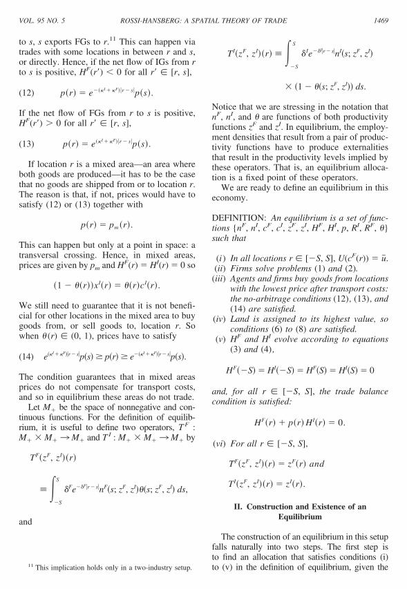
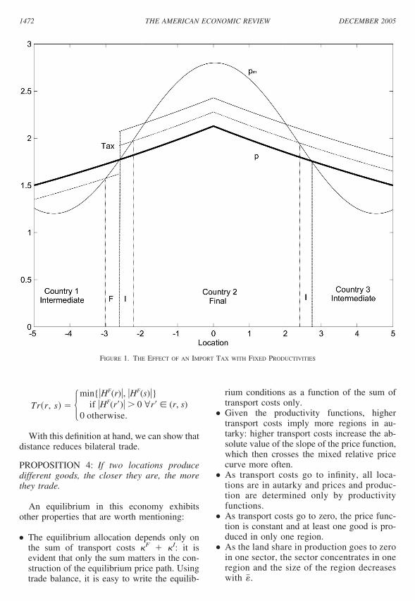
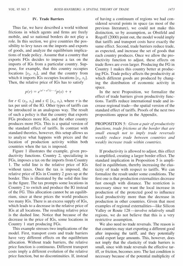
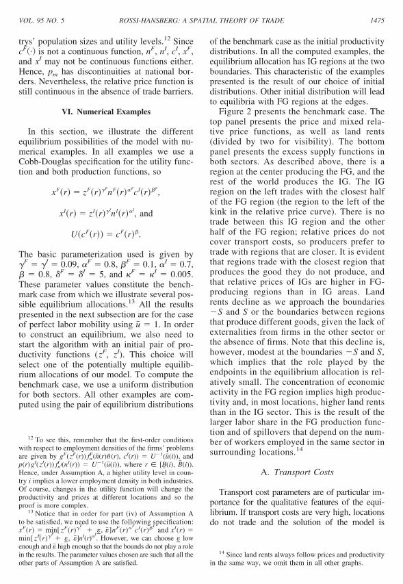
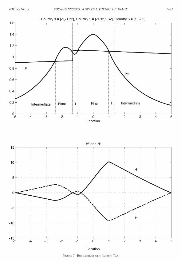
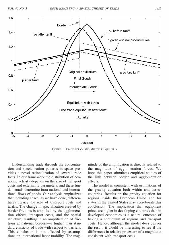