authors.library.caltech.eduA SPARSE DECOMPOSITION OF LOW RANK SYMMETRIC POSITIVE SEMI-DEFINITE...
33
A SPARSE DECOMPOSITION OF LOW RANK SYMMETRIC POSITIVE SEMI-DEFINITE MATRICES THOMAS Y. HOU, QIN LI, AND PENGCHUAN ZHANG Abstract. Suppose that A ∈ R N×N is symmetric positive semidefinite with rank K ≤ N . Our goal is to decompose A into K rank-one matrices ∑ K k=1 g k g T k where the modes {g k } K k=1 are required to be as sparse as possible. In contrast to eigen decomposition, these sparse modes are not required to be orthogonal. Such a problem arises in random field parametrization where A is the covariance function and is intractable to solve in general. In this paper, we partition the indices from 1 to N into several patches and propose to quantify the sparseness of a vector by the number of patches on which it is nonzero, which is called patch- wise sparseness. Our aim is to find the decomposition which minimizes the total patch-wise sparseness of the decomposed modes. We propose a domain-decomposition type method, called intrinsic sparse mode decomposition (ISMD), which follows the “local-modes-construction + patching-up” procedure. The key step in the ISMD is to construct local pieces of the intrinsic sparse modes by a joint diagonalization problem. Thereafter a pivoted Cholesky decomposition is utilized to glue these local pieces together. Optimal sparse decomposition, consistency with different domain decomposition and robustness to small perturbation are proved under the so called regular-sparse assumption (see Definition 1.2). We provide simulation results to show the efficiency and robustness of the ISMD. We also compare the ISMD to other existing methods, e.g., eigen decomposition, pivoted Cholesky decomposition and convex relaxation of sparse principal component analysis [25, 40]. 1. Introduction Many problems in science and engineering lead to huge symmetric and positive semi-definite (PSD) matrices. Often they arise from the discretization of self-adjoint PSD operators or their kernels, especially in the context of data science and partial differential equations. Consider a symmetric PSD matrix of size N × N , denoted as A. Since N is typically large, this causes serious obstructions when dealing numerically with such problems. Fortunately in many applications the discretization A is low-rank or approximately low-rank, i.e., there exists {ψ 1 ,...,ψ K }⊂ R N for K N such that A = K X k=1 ψ k ψ T k or kA - K X k=1 ψ k ψ T k k 2 ≤ , respectively. Here, > 0 is some small number and kAk 2 = λ max (A) is the largest eigenvalue of A. To obtain such a low-rank decomposition/approximation of A, the most natural method is perhaps the eigen decomposition with {ψ k } K k=1 as the eigenvectors corresponding to the largest K eigenvalues of A. An additional advantage of the eigen decomposition is the fact that eigenvectors are orthogonal to each other. However, eigenvectors are typically dense vectors, i.e., every entry is typically nonzero. For a symmetric PSD matrix A with rank K N , the aim of this paper is to find an alternative decomposition (1) A = K X k=1 g k g T k . Here the number of components is still its rank K, which is optimal, and the modes {g k } K k=1 are required to be as sparse as possible. In this paper, we work on the symmetric PSD matrices, which are typically the discretized self-adjoint PSD operators or their kernels. We couldhave just as well worked on the self-adjoint Date : December 7, 2016. Applied and Comput. Math, Caltech, Pasadena, CA 91125. Email: [email protected]. Math, UW-Madison, Madison, WI 53705. Email: [email protected]. Applied and Comput. Math, Caltech, Pasadena, CA 91125. Email: [email protected]. 1 arXiv:1607.00702v2 [math.NA] 5 Dec 2016
Transcript of authors.library.caltech.eduA SPARSE DECOMPOSITION OF LOW RANK SYMMETRIC POSITIVE SEMI-DEFINITE...
A SPARSE DECOMPOSITION OF LOW RANK SYMMETRIC POSITIVE
SEMI-DEFINITE MATRICES
THOMAS Y. HOU, QIN LI, AND PENGCHUAN ZHANG
Abstract. Suppose that A ∈ RN×N is symmetric positive semidefinite with rank K ≤ N . Our goal is to
decompose A into K rank-one matrices∑K
k=1 gkgTk where the modes gkKk=1 are required to be as sparse
as possible. In contrast to eigen decomposition, these sparse modes are not required to be orthogonal. Such
a problem arises in random field parametrization where A is the covariance function and is intractable to
solve in general. In this paper, we partition the indices from 1 to N into several patches and propose toquantify the sparseness of a vector by the number of patches on which it is nonzero, which is called patch-
wise sparseness. Our aim is to find the decomposition which minimizes the total patch-wise sparseness of
the decomposed modes. We propose a domain-decomposition type method, called intrinsic sparse modedecomposition (ISMD), which follows the “local-modes-construction + patching-up” procedure. The key
step in the ISMD is to construct local pieces of the intrinsic sparse modes by a joint diagonalization problem.
Thereafter a pivoted Cholesky decomposition is utilized to glue these local pieces together. Optimal sparsedecomposition, consistency with different domain decomposition and robustness to small perturbation are
proved under the so called regular-sparse assumption (see Definition 1.2). We provide simulation results to
show the efficiency and robustness of the ISMD. We also compare the ISMD to other existing methods, e.g.,eigen decomposition, pivoted Cholesky decomposition and convex relaxation of sparse principal component
analysis [25, 40].
1. Introduction
Many problems in science and engineering lead to huge symmetric and positive semi-definite (PSD)matrices. Often they arise from the discretization of self-adjoint PSD operators or their kernels, especiallyin the context of data science and partial differential equations.
Consider a symmetric PSD matrix of size N × N , denoted as A. Since N is typically large, this causesserious obstructions when dealing numerically with such problems. Fortunately in many applications thediscretization A is low-rank or approximately low-rank, i.e., there exists ψ1, . . . , ψK ⊂ RN for K Nsuch that
A =
K∑k=1
ψkψTk or ‖A−
K∑k=1
ψkψTk ‖2 ≤ ε,
respectively. Here, ε > 0 is some small number and ‖A‖2 = λmax(A) is the largest eigenvalue of A. Toobtain such a low-rank decomposition/approximation of A, the most natural method is perhaps the eigendecomposition with ψkKk=1 as the eigenvectors corresponding to the largest K eigenvalues of A. Anadditional advantage of the eigen decomposition is the fact that eigenvectors are orthogonal to each other.However, eigenvectors are typically dense vectors, i.e., every entry is typically nonzero.
For a symmetric PSD matrix A with rank K N , the aim of this paper is to find an alternativedecomposition
(1) A =
K∑k=1
gkgTk .
Here the number of components is still its rank K, which is optimal, and the modes gkKk=1 are requiredto be as sparse as possible. In this paper, we work on the symmetric PSD matrices, which are typically thediscretized self-adjoint PSD operators or their kernels. We could have just as well worked on the self-adjoint
Date: December 7, 2016.Applied and Comput. Math, Caltech, Pasadena, CA 91125. Email: [email protected], UW-Madison, Madison, WI 53705. Email: [email protected].
Applied and Comput. Math, Caltech, Pasadena, CA 91125. Email: [email protected].
1
arX
iv:1
607.
0070
2v2
[m
ath.
NA
] 5
Dec
201
6
2 THOMAS Y. HOU, QIN LI, AND PENGCHUAN ZHANG
PSD operators. This would correspond to the case when N = ∞. Much of what will be discussed belowapplies equally well to this case.
Symmetric PSD matrices/operators/kernels appear in many science and engineering branches and variousefforts have been made to seek sparse modes. In statistics, sparse Principal Component Analysis (PCA) andits convex relaxations [20, 46, 8, 40] are designed to sparsify the eigenvectors of data covariance matrices. Inquantum chemistry, Wannier functions [42, 23] and other methods [34, 43, 33, 37, 25] have been developed toobtain a set of functions that approximately span the eigenspace of the Hamitonian, but are spatially localizedor sparse. In numerical homogenization of elliptic equations with rough coefficients [14, 15, 9, 36, 35], a set ofmultiscale basis functions is constructed to approximate the eigenspace of the elliptic operator and is used asthe finite element basis to solve the equation. In most cases, sparse modes reduce the computational cost forfurther scientific experiments. Moreover, in some cases sparse modes have a better physical interpretationcompared to the global eigen-modes. Therefore, it is of practical importance to obtain sparse (localized)modes.
1.1. Our results. The number of nonzero entries of a vector ψ ∈ RN is called its l0 norm, denoted by‖ψ‖0. Since the modes in (1) are required to be as sparse as possible, the sparse decomposition problem isnaturally formulated as the following optimization problem
(2) minψ1,...,ψK∈RN
K∑k=1
‖ψk‖0 s.t. A =
K∑k=1
ψkψTk .
However, this problem is rather difficult to solve because: first, minimizing l0 norm results in a combinatorialproblem and is computationally intractable in general; second, the number of unknown variables is K ×Nwhere N is typically a huge number. Therefore, we introduce the following patch-wise sparseness as asurrogate of ‖ψk‖0 and make the problem computationally tractable.
Definition 1.1 (Patch-wise sparseness). Suppose that P = PmMm=1 is a disjoint partition of the N nodes,i.e., [N ] ≡ 1, 2, 3, . . . , N = tMm=1Pm. The patch-wise sparseness of ψ ∈ RN with respect to the partitionP, denoted by s(ψ;P), is defined as
s(ψ;P) = #P ∈ P : ψ|P6= 0.
Throughout this paper, [N ] denotes the index set 1, 2, 3, . . . , N; 0 denotes the vectors with all entriesequal to 0; |P | denotes the cardinality of a set P ; ψ|
P∈ R|P | denotes the restriction of ψ ∈ RN on patch
P . Once the partition P is fixed, smaller s(ψ;P) means that ψ is nonzero on fewer patches, which implies asparser vector. With patch-wise sparseness as a surrogate of the l0 norm, the sparse decomposition problem(2) is relaxed to
(3) minψ1,...,ψK∈RN
K∑k=1
s(ψk;P) s.t. A =
K∑k=1
ψkψTk .
If gkKk=1 is an optimizer for (3), we call them a set of intrinsic sparse modes for A under partition P. Sincethe objective function of problem (3) only takes nonnegative integer values, we know that for a symmetricPSD matrix A with rank K, there exists at least one set of intrinsic sparse modes.
It is obvious that the intrinsic sparse modes depend on the domain partition P. Two extreme caseswould be M = N and M = 1. For M = N , s(ψ;P) recovers ‖ψ‖0 and the patch-wise sparseness mini-mization problem (3) recovers the original l0 minimization problem (2). Unfortunately, it is computationallyintractable. For M = 1, every non-zero vector has sparseness one, and thus the number of nonzero entriesmakes no difference. However, in this case the problem (3) is computationally tractable. For instance, aset of (unnormalized) eigenvectors is one of the optimizers. We are interested in the sparseness defined inbetween, namely, a partition with a meso-scale patch size. Compared to ‖ψ‖0, the meso-scale partitionsacrifices some resolution when measuring the support, but makes the optimization (3) efficiently solvable.Specifically, Problem (3) with the following regular-sparse partitions enjoys many good properties. Theseproperties enable us to design a very efficient algorithm to solve Problem (3).
Definition 1.2 (regular-sparse partition). The partition P is regular-sparse with respect to A if there exists
a decomposition A =∑Kk=1 gkg
Tk such that all nonzero modes on each patch Pm are linearly independent.

A SPARSE DECOMPOSITION OF LOW RANK SYMMETRIC POSITIVE SEMI-DEFINITE MATRICES 3
If two intrinsic sparse modes are non-zero on exactly the same set of patches, which are called unidentifiablemodes in Definition 3.2, it is easy to see that any rotation of these unidentifiable modes forms another set ofintrinsic sparse modes. From a theoretical point of view, if a partition is regular-sparse with respect to A, theintrinsic sparse modes are unique up to rotations of unidentifiable modes, see Theorem 3.1. Moreover, as thepartition gets refined, the original identifiable intrinsic sparse modes remain unchanged, while the originalunidentifiable modes become identifiable and become sparser (in the sense of l0 norm), see Theorem 3.2. Inthis sense, the intrinsic sparse modes are independent of the partition that we use. From a computationalpoint of view, a regular-sparse partition ensures that the restrictions of the intrinsic sparse modes on eachpatch Pm can be constructed from rotations of local eigenvectors. Following this idea, we propose theintrinsic sparse mode decomposition (ISMD), see Algorithm 1. In Theorem 3.1, we have proved that theISMD solves problem (3) exactly on regular-sparse partitions. We point out that, even when the partition isnot regular-sparse, numerical experiments show that the ISMD still generates a sparse decomposition of A.
The ISMD consists of three steps. In the first step, we perform eigen decomposition of A restrictedon local patches PmMm=1, denoted as AmmMm=1, to get Amm = HmH
Tm. Here, columns of Hm are
the unnormalized local eigenvectors of A on patch Pm. In the second step, we recover the local pieces ofintrinsic sparse modes, denoted by Gm, by rotating the local eigenvectors Gm = HmDm. The method tofind the right local rotations DmMm=1 is the core of the ISMD. All the local rotations are coupled by the
decomposition constraint A =∑Kk=1 gkg
Tk and it seems impossible to solve DmMm=1 from this big coupled
system. Surprisingly, when the partition is regular-sparse, this coupled system can be decoupled and everylocal rotation Dm can be solved independently by a joint diagonalization problem (13). In the last “patch-up”step, we identify correlated local pieces across different patches by the pivoted Cholesky decomposition of asymmetric PSD matrix Ω and then glue them into a single intrinsic sparse mode. Here, Ω is the projectionof A onto the subspace spanned by all the local pieces GmMm=1, see Eqn. (15). This step is necessary toreduce the number of decomposed modes to the optimal K, i.e., the rank of A. The last step also equips theISMD the power to identify long range correlation and to honor the intrinsic correlation structure hidden inA. The popular l1 approach typically does not have this property.
The ISMD has very low computational complexity. There are two reasons for its efficiency: first of all,instead of computing the expensive global eigen decomposition, we compute only the local eigen decomposi-tions of AmmMm=1; second, there is an efficient algorithm to solve the joint diagonalization problems for thelocal rotations DmMm=1. Moreover, because both performing the local eigen decompositions and solvingthe joint diagonalization problems can be done independently on each patch, the ISMD is embarrassinglyparallelizable.
The stability of the ISMD is also explored when the input data A is mixed with noises. We study the
small perturbation case, i.e., A = A + εA. Here, A is the noiseless rank-K symmetric PSD matrix, A isthe symmetric additive perturbation and ε > 0 quantifies the noise level. A simple thresholding step is
introduced in the ISMD to achieve our aim: to clean up the noise εA and to recover the intrinsic sparsemodes of A. Under some assumptions, we can prove that sparse modes gkKk=1, produced by the ISMD withthresholding, exactly capture the supports of A’s intrinsic sparse modes gkKk=1 and the error ‖gk − gk‖ issmall. See Section 4.1 for a precise description.
We have verified all the theoretical predictions with numerical experiments on several synthetic covariancematrices of high dimensional random vectors. Without parallel execution, for partitions with a large range ofpatch sizes, the computational cost of the ISMD is comparable to that of the partial eigen decomposition [38,28]. For certain partitions, the ISMD could be 10 times faster than the partial eigen decomposition. Wehave also implemented the convex relaxation of sparse PCA [25, 40] and compared these two methods. Itturns out that the convex relaxation of sparse PCA fails to capture the long range correlation, needs toperform (partial) eigen decomposition on matrices repeatedly for many times and is thus much slower thanthe ISMD. Moreover, we demonstrate the robustness of the ISMD on partitions which are not regular-sparseand on inputs which are polluted with small noises.
1.2. Applications. The ISMD leads to a sparse-orthogonal matrix factorization for any matrix. Given amatrix X ∈ RN×M of rank K and a partition P of the index set [N ], the ISMD tries to solve the following

4 THOMAS Y. HOU, QIN LI, AND PENGCHUAN ZHANG
optimization problem:
(4) ming1,...,gK∈RN
u1,...,uK∈RM
K∑k=1
s(gk;P) s.t. X =
K∑k=1
gkuTk , uTk uk′ = δk,k′ ∀1 ≤ k, k′ ≤ K,
where s(gk;P) is the patch-wise sparseness defined in Definition (1.1). Compared to the bi-orthogonalproperty of SVD, the ISMD requires orthogonality only in one dimension and requires sparsity in the otherdimension. The method to obtain the decomposition (4) consists of three steps: first, compute A = XXT ;second, apply the ISMD to A to get gkKk=1; third, project X on to gkKk=1 to obtain ukKk=1.
The sparse-orthogonal matrix factorization (4) has potential applications in statistics, machine learningand uncertainty quantification. In statistics and machine learning, latent factor models with sparse loadingshave found many applications ranging from DNA microarray analysis [11], facial and object recognition [41],web search models [1] and etc. Specifically, latent factor models decompose a data matrix X ∈ RN×M byproduct of the loading matrix G ∈ RN×K and the factor value matrix U ∈ RM×K , with possibly small noiseE ∈ RN×M , i.e.,
(5) X = GUT + E.
The sparse-orthogonal matrix factorization (4) tries to find the optimal sparse loadings G under the conditionthat latent factors are normalized and uncorrelated, i.e., columns in U are orthonormal. In practice, theuncorrelated latent factors make lots of sense, but is not guaranteed by many existing matrix factorizationmethods, e.g., non-negative matrix factorization (NMF) [26], sparse PCA [20, 46, 8], structured sparsePCA [19].
In uncertainty quantification (UQ), we often need to parametrize a random field, denoted as κ(x, ω), witha finite number of random variables. Applying the ISMD to its covariance function, denoted by Cov(x, y),we can get a parametrization with K random variables:
(6) κ(x, ω) = κ(x) +
K∑k=1
gk(x)ηk(ω),
where κ(x) is the mean field, the physical modes gkKk=1 are sparse/localized, and the random variablesηkKk=1 are centered, uncorrelated, and have unit variance. The parametrization (6) has a form similarto the widely used Karhenen-Loeve (KL) expansion [22, 29], but in the KL expansion the physical modesgkKk=1 are eigenfunctions of the covariance function and are typically nonzero everywhere. Obtaining asparse parametrization is important to uncover the intrinsic sparse feature in a random field and to achievecomputational efficiency for further scientific experiments. In [16], such sparse parametrization methods areused to design efficient algorithms to solve partial differential equations with random inputs.
1.3. Connection with the sparse matrix factorization problem. Given a matrix X ∈ RN×M of Mcolumns corresponding to M observations in RN , a sparse matrix factorization problem is to find a matrixG = [g1, . . . , gr] ∈ RN×r, called dictionary, and a matrix U = [u1, . . . , ur] ∈ RM×r, called decompositioncoefficients, such that GUT approximates X well and the columns in G are sparse.
In [27, 44, 32], the authors formulated this problem as an optimization problem by penalizing the l1 normof G, i.e. ‖G‖1 :=
∑rk=1 ‖gk‖1, to enforce the sparsity of the dictionary. This can be written as
(7) minG∈RN×r,U∈RM×r
‖X −GUT ‖2F + λ‖G‖1 s.t. ‖uk‖2 ≤ 1 ∀1 ≤ k ≤ r,
where the parameter λ > 0 controls to what extent the dictionary G is regularized. We point out that the l1penalty can be replaced by other penalties. For example, the structured sparse PCA [19] uses certain l1/l2norm of G to enforce sparsity with specific structures, e.g. rectangular structure on a grid. Problem (7)is not jointly convex in (G,U). Certain specially designed algorithms have been developed to solve thisoptimization problem. We will discuss one of these methods in Section 2.3.
There are two major differences between the optimization problem (4) and the optimization problem (7).First, the ISMD, which is designed to solve (4), requires that the decomposition coefficients U be orthonormal,while many other methods, including sparse PCA and structured sparse PCA, which are designed to solve (7),only normalize every columns in U . One needs to decide whether the orthogonality in U is necessary in her
A SPARSE DECOMPOSITION OF LOW RANK SYMMETRIC POSITIVE SEMI-DEFINITE MATRICES 5
application and choose the appropriate method. Second, the number of modes K in the ISMD must bethe rank of the matrix, while the number of modes r in problem (7) is picked by users and can be anynumber. In other words, the ISMD is seeking an exact matrix decomposition, while other methods make atrade-off between the accuracy ‖X −GUT ‖F and the sparsity ‖G‖1 by recovering the matrix approximatelyinstead of obtaining an exact recovery. Although the ISMD can be modified to do matrix approximation(with the orthogonality constraint on U), see Algorithm 3, the optimal sparsity of the dictionary G is notguaranteed anymore. Based on these two differences, we recommend the ISMD for sparse matrix factorizationproblems where the orthogonality in decomposition coefficients U is required and an exact (or nearly exact)decomposition is desired. In our upcoming paper [17, 18], we will present our recent results on solvingProblem (7).
1.4. Outlines. In Section 2 we present our ISMD algorithm for low rank matrices, analyze its computationalcomplexity and talk about its relation with other methods for sparse decomposition or approximation.In Section 3 we present our main theoretical results, i.e., Theorem 3.1 and Theorem 3.1. In Section 4,we discuss the stability of the ISMD by performing perturbation analysis. We also provide two modifiedISMD algorithms: Algorithm 2 for low rank matrix with small noise, and Algorithm 3 for sparse matrixapproximation. Finally, we present a few numerical examples in Section 5 to demonstrate the efficiency ofthe ISMD and compare its performance with other existing methods.
2. Intrinsic Sparse Mode Decomposition
In this section, we present the algorithm of the ISMD and analyze its computational complexity. Itsrelation with other matrix decomposition methods is discussed in the end of this section. In the rest of thepaper, O(n) denotes the set of real unitary matrices of size n × n; In denotes the identity matrix with sizen× n.
2.1. ISMD. Suppose that we have one symmetric positive symmetric matrix, denoted as A ∈ RN×N , anda partition of the index set [N ], denoted as P = PmMm=1. The partition typically originates from thephysical meaning of the matrix A. For example, if A is the discretized covariance function of a random fieldon domain D ⊂ Rd, P is constructed from certain domain partition of D. The submatrix of A, with rowindex in Pm and column index in Pn, is denoted as Amn. To simplify our notations, we assume that indicesin [N ] are rearranged such that A is written as below:
A =
A11 A12 · · · A1M
A21 A22 · · · A2M
......
. . ....
AM1 AM2 · · · AMM
.(8)
Notice that when implementing the ISMD, there is no need to rearrange the indices as above. The ISMD triesto find the optimal sparse decomposition of A w.r.t. partition P, defined as the minimizer of problem (3).The ISMD consists of three steps: local decomposition, local rotation, and global patch-up.
In the first step, we perform eigen decomposition
(9) Amm =
Km∑i=1
γm,ihm,ihTm,i ≡ HmH
Tm,
where Km is the rank of Amm and Hm = [γ1/2m,1hm,i , γ
1/2m,2hm,2 , . . . γ
1/2m,Km
hm,Km]. If Amm is ill-conditioned,
we truncate the small eigenvalues and a truncated eigen decomposition is used as follows:
(10) Amm ≈Km∑i=1
γm,ihm,ihTm,i ≡ HmH
Tm.
Let K(t) ≡∑Mm=1Km be the total local rank of A. We extend columns of Hm into RN by adding zeros,
and get the block diagonal matrix
Hext = diagH1, H2, · · · , HM.
6 THOMAS Y. HOU, QIN LI, AND PENGCHUAN ZHANG
The correlation matrix with basis Hext, denoted by Λ ∈ RK(t)×K(t) , is the matrix such that
(11) A = HextΛHText.
Since columns of Hext are orthogonal and span a space that contains range(A), Λ exists and can be computedblock-wisely as follows:
Λ =
Λ11 Λ12 · · · Λ1M
Λ21 Λ22 · · · Λ2M
......
. . ....
ΛM1 ΛM2 · · · ΛMM
, Λmn = H†mAmn(H†n)T ∈ RKm×Kn .(12)
where H†m ≡ (HTmHm)−1HT
m is the (Moore-Penrose) pseudo-inverse of Hm.In the second step, on every patch Pm, we solve the following joint diagonaliziation problem to find a
local rotation Dm:
(13) minV ∈O(Km)
M∑n=1
∑i6=j
|(V TΣn;mV )i,j |2 ,
in which
(14) Σn;m ≡ ΛmnΛTmn.
We rotate the local eigenvectors with Dm and get Gm = HmDm. Again, we extend columns of Gm into RNby adding zeros, and get the block diagonal matrix
Gext = diagG1, G2, · · · , GM.
The correlation matrix with basis G, denoted by Ω ∈ RK(t)×K(t) , is the matrix such that
(15) A = GextΩGText.
With Λ in hand, Ω can be obtained as follows:
(16) Ω = DTΛD , D = diagD1, D2, · · · , DM.
Joint diagonalization has been well studied in the blind source separation (BSS) community. We presentsome relevant theoretical results in Appendix C. A Jacobi-like algorithm [4, 2], see Algorithm 4, is used inour paper to solve problem (13). For most cases, we may want to normalize the columns of Gext and put allthe magnitude information in Ω, i.e.,
(17) Gext = GextE, Ω = EΩET ,
where E is a diagonal matrix with Eii being the l2 norm of the i-th column of Gext, Gext and Ω will substitutethe roles of G and Ω in the rest of the algorithm.
In the third step, we use the pivoted Cholesky decomposition to patch up the local pieces Gm. Specifically,suppose the pivoted Cholesky decomposition of Ω is given as
(18) Ω = PLLTPT ,
where P ∈ RK(t)×K(t) is a permutation matrix and L ∈ RK(t)×K is a lower triangular matrix with positivediagonal entries. Since A has rank K, both Λ and Ω have rank K. This is why L only has K nonzerocolumns. However, we point out that the rank K is automatically identified in the algorithm instead ofgiven as an input parameter. Finally, A is decomposed as
(19) A = GGT ≡ GextPL(GextPL)T .
The columns in G (GextPL) are our decomposed sparse modes.The full algorithm is summarized in Algorithm 1. We point out that there are two extreme cases for the
ISMD:
• The coarsest partition P = [N ]. In this case, the ISMD is equivalent to the standard eigendecomposition.
A SPARSE DECOMPOSITION OF LOW RANK SYMMETRIC POSITIVE SEMI-DEFINITE MATRICES 7
• The finest partition P = i : i ∈ [N ]. In this case, the ISMD is equivalent to the pivoted Cholesky
factorization on A where Aij =Aij√AiiAjj
. If the normalization (17) is applied, the ISMD is equivalent
to the pivoted Cholesky factorization of A in this case.
In these two extreme cases, there is no need to use the joint diagonalization step and it is known that ingeneral neither the ISMD nor the pivoted Cholesky decomposition generates sparse decomposition. WhenP is neither of these two extreme cases, the joint diagonalization is applied to rotate the local eigenvectorsand thereafter the generated modes are patch-wise sparse. Specifically, when the partition is regular-sparse,the ISMD generates the optimal patch-wise sparse decomposition as stated in Theorem 3.1.
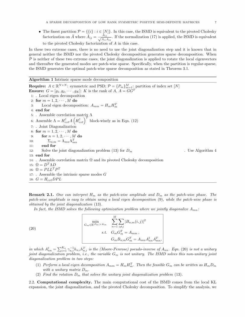
Algorithm 1 Intrinsic sparse mode decomposition
Require: A ∈ RN×N : symmetric and PSD; P = PmMm=1: partition of index set [N ]Ensure: G = [g1, g2, · · · , gK ]: K is the rank of A, A = GGT
1: . Local eigen decomposition2: for m = 1, 2, · · · ,M do3: Local eigen decomposition: Amm = HmH
Tm
4: end for5: . Assemble correlation matrix Λ
6: Assemble Λ = H†extA(H†ext
)Tblock-wisely as in Eqn. (12)
7: . Joint Diagonalization8: for m = 1, 2, · · · ,M do9: for n = 1, 2, · · · ,M do
10: Σn;m = ΛmnΛTmn11: end for12: Solve the joint diagonalization problem (13) for Dm . Use Algorithm 413: end for14: . Assemble correlation matrix Ω and its pivoted Cholesky decomposition15: Ω = DTΛD16: Ω = PLLTPT
17: . Assemble the intrinsic sparse modes G18: G = HextDPL
Remark 2.1. One can interpret Hm as the patch-wise amplitude and Dm as the patch-wise phase. Thepatch-wise amplitude is easy to obtain using a local eigen decomposition (9), while the patch-wise phase isobtained by the joint diagonalization (13).
In fact, the ISMD solves the following optimization problem where we jointly diagonalize Amn:
(20)
minGm∈R|Pm|×Km
M∑n=1
∑i 6=j
|Bn;m(i, j)|2
s.t. GmGTm = Amm ,
GmBn;mGTm = AmnA
†nnA
Tmn,
in which A†nn =∑Kn
i=1 γ−1n,ihn,ih
Tn,i is the (Moore-Penrose) pseudo-inverse of Ann. Eqn. (20) is not a unitary
joint diagonalization problem, i.e., the variable Gm is not unitary. The ISMD solves this non-unitary jointdiagonalization problem in two steps:
(1) Perform a local eigen decomposition Amm = HmHTm. Then the feasible Gm can be written as HmDm
with a unitary matrix Dm.(2) Find the rotation Dm that solves the unitary joint diagonalization problem (13).
2.2. Computational complexity. The main computational cost of the ISMD comes from the local KLexpansion, the joint diagonalization, and the pivoted Cholesky decomposition. To simplify the analysis, we

8 THOMAS Y. HOU, QIN LI, AND PENGCHUAN ZHANG
assume that the partition P is uniform, i.e., each group has NM nodes. On each patch, we perform eigen
decomposition of Amm of size N/M and rank Km. Then, the cost of the local eigen decomposition step is
Cost1 =
M∑m=1
O((N/M)2Km
)= (N/M)2O(
M∑m=1
Km).
For the joint diagonalization, the computational cost of Algorithm 4 is
M∑m=1
Ncorr,mK3mNiter,m .
Here, Ncorr,m is the number of nonzero matrices in Σn;mMn=1. Notice that Σn;m ≡ ΛmnΛTmn = 0 if and onlyif Amn = 0. Therefore, Ncorr,m may be much smaller than M if A is sparse. Nevertheless, we take an upperbound M to estimate the cost. Ncorr,mK
3m is the computational cost for each sweeping in Algorithm 4 and
Niter,m is the number of iterations needed for the convergence. The asymptotic convergence rate is shownto be quadratic [2], and we see no more than 6 iterations needed in our numerical examples. Therefore, wecan take Niter,m = O(1) and in total we have
Cost2 =
M∑m=1
MO(K3m) = MO(
M∑m=1
K3m).
Finally, the pivoted Cholesky decomposition of Ω, which is of size∑Mk=1Km, has cost
Cost3 = O
((
M∑k=1
Km)K2
)= K2O(
M∑m=1
Km).
Combining the computational costs in all three steps, we conclude that the total computational cost of theISMD is
(21) CostISMD =((N/M)2 +K2
)O(
M∑m=1
Km) +MO(
M∑m=1
K3m) .
Making use of Km ≤ K, we have an upper bound for CostISMD
(22) CostISMD ≤ O(N2K/M) +O(M2K3) .
When M = O((N/K)2/3), CostISMD ≤ O(N4/3K5/3). Comparing to the cost of partial eigen decomposi-tion [38, 28], which is about O(N2K) 1, the ISMD is more efficient for low-rank matrices.
For matrix A which has a sparse decomposition, the local ranks Km are much smaller than its global rankK. An extreme case is Km = O(1), which is in fact true for many random fields, see [7, 16]. In this case,
(23) CostISMD = O(N2/M) +O(M2) +O(MK2) .
When the partition gets finer (M increases), the computational cost first decreases due to the saving inlocal eigen decompositions. The computational cost achieves its minimum around M = O(N2/3) and thenincreases due to the increasing cost for the joint diagonalization. This trend is observed in our numericalexamples, see Figure 4.
We point out that the M local eigen decompositions (9) and the joint diagonalization problems (13) aresolved independently on different patches. Therefore, our algorithm is embarrassingly parallelizable. Thiswill save the computational cost in the first two steps by a factor of M , which makes the ISMD even faster.
2.3. Connection with other matrix decomposition methods. Sparse decompositions of symmetricPSD matrices have been studied in different fields for a long time. There are in general two approaches toachieve sparsity: rotation or L1 minimization.
The rotation approach begins with eigenvectors. Suppose that we have decided to retain and rotate Keigenvectors. Define H = [h1, h2, . . . , hK ] with hk being the k-th eigenvector. We post-multiply H by amatrix T ∈ RK×K to obtain the rotated modes G = [g1, g2, . . . , gK ] = HT . The choice of T is determinedby the rotation criterion we use. In data science, for the commonly-used varimax rotation criterion [24, 21],T is an orthogonal matrix chosen to maximize the variance of squared modes within each column of G.
1The cost can be reduced to O(N2 log(K)) if a randomized SVD with some specific technique is applied.

A SPARSE DECOMPOSITION OF LOW RANK SYMMETRIC POSITIVE SEMI-DEFINITE MATRICES 9
This drives entries in G towards 0 or ±1. In quantum chemistry, every column in H and G corresponds toa function over a physical domain D and certain specialized sparse modes – localized modes – are soughtafter. The most widely used criterion to achieve maximally localized modes is the one proposed in [34]. Thiscriterion requires T to be unitary, and then minimizes the second moment:
(24)
K∑k=1
∫D
(x− xk)2|gk(x)|2dx ,
where xk =∫Dx|gk(x)|2dx. More recently, a method weighted by higher degree polynomials is discussed in
[43]. While these criteria work reasonably well for simple symmetric PSD functions/operators, they all sufferfrom non-convex optimization – which requires a good starting point to converge to the global minimum.In addition, these methods only care about the eigenspace spanned by H instead of the specific matrixdecomposition, and thus they cannot be directly applied to solve our problem (3).
The ISMD proposed in this paper follows the rotation approach. The ISMD implicitly finds a unitarymatrix T ∈ RK×K to construct the intrinsic sparse modes
(25) [g1, g2, . . . , gK ] = [√λ1h1,
√λ2h2, . . . ,
√λKhK ] T.
Notice that we rotate the unnormalized eigenvector√λkhk to satisfy the decomposition constraint A =∑K
k=1 gkgTk . The criterion of the ISMD is to minimize the total patch-wise sparseness as in (3). The success
of the ISMD lies in the fact that as long as the domain partition is regular-sparse, the optimization problem (3)can be exactly and efficiently solved by Algorithm 1. Moreover, the intrinsic sparse modes produced by theISMD are optimally localized because we are directly minimizing the total patch-wise sparseness of gkKk=1.
The L1 minimization approach, pioneered by ScotLass [20], has a rich literature in solving the sparsematrix factorization problem (7), see [46, 8, 45, 40, 37, 25]. Problem (7) is highly non-convex in (G,U), andthere has been a lot of efforts (see e.g. [8, 40, 25]) in relaxing it to a convex optimization. First of all, sincethere are no essential constraints on U , one can get rid of U by considering the variational form [20, 46, 37]:
(26) minG∈RN×K
−Tr(GTAG) + µ‖G‖1 s.t. GTG = IK ,
where A = XXT is the covariance matrix as in the ISMD (3) and Tr is the trace operator on square matrices.Notice that the problem is still non-convex due to the orthogonality constraint GTG = IK . In the secondstep, the authors in [40] proposed the following semi-definite programming to obtain the sparse densitymatrix W ∈ Rn×n, which plays the same role as GGT in (26):
(27) minW∈RN×N
−Tr(AW ) + µ‖W‖1 s.t. 0 W IN , Tr(W ) = K.
Here, 0 W IN means that both W and IN −W are symmetric and positive semi-definite. Finally, thefirst K eigenvectors of W are used as the sparse modes G. An equivalent formulation was proposed in [25],and the authors proposed to pick K columns of W as the sparse modes G.
We will compare the advantages and disadvantages of the ISMD and the convex relaxation of sparse PCAin Section 5.2 and Section 5.6.
3. Theoretical results with regular-sparse partitions
In this section, we present the main theoretical results of the ISMD, i.e., Theorem 3.1, Theorem 3.2and its perturbation analysis. We first introduce a domain-decomposition type presentation of any feasible
decomposition A =∑Kk=1 ψkψ
Tk . Then we discuss the regular-sparse property and use it to prove our main
results. When no ambiguity arises, we denote patch-wise sparseness s(gk;P) as sk.
3.1. A domain-decomposition type presentation. For an arbitrary decomposition A =∑Kk=1 ψkψ
Tk ,
denote Ψ ≡ [ψ1, . . . , ψK ] and Ψ|Pm≡ [ψ1|Pm
, . . . , ψK |Pm]. For a sparse decomposition, we expect that most
columns in Ψ|Pm
are zero, and thus we define the local dimension on patch Pm as follows.
Definition 3.1 (Local dimension). The local dimension of a decomposition A =∑Kk=1 ψkψ
Tk on patch Pm
is the number of nonzero modes when restricted to this patch, i.e.,
d(Pm; Ψ) = |Sm|, Sm = k : ψk|Pm6= 0.
10 THOMAS Y. HOU, QIN LI, AND PENGCHUAN ZHANG
0 0.1 0.2 0.3 0.4 0.5 0.6 0.7 0.8 0.9 1−0.1
0
0.1
0.2
0.3
0.4
d1 = 1
d2 = 2 d
3 = 1
d4 = 1
s1 = 2
s2 = 3
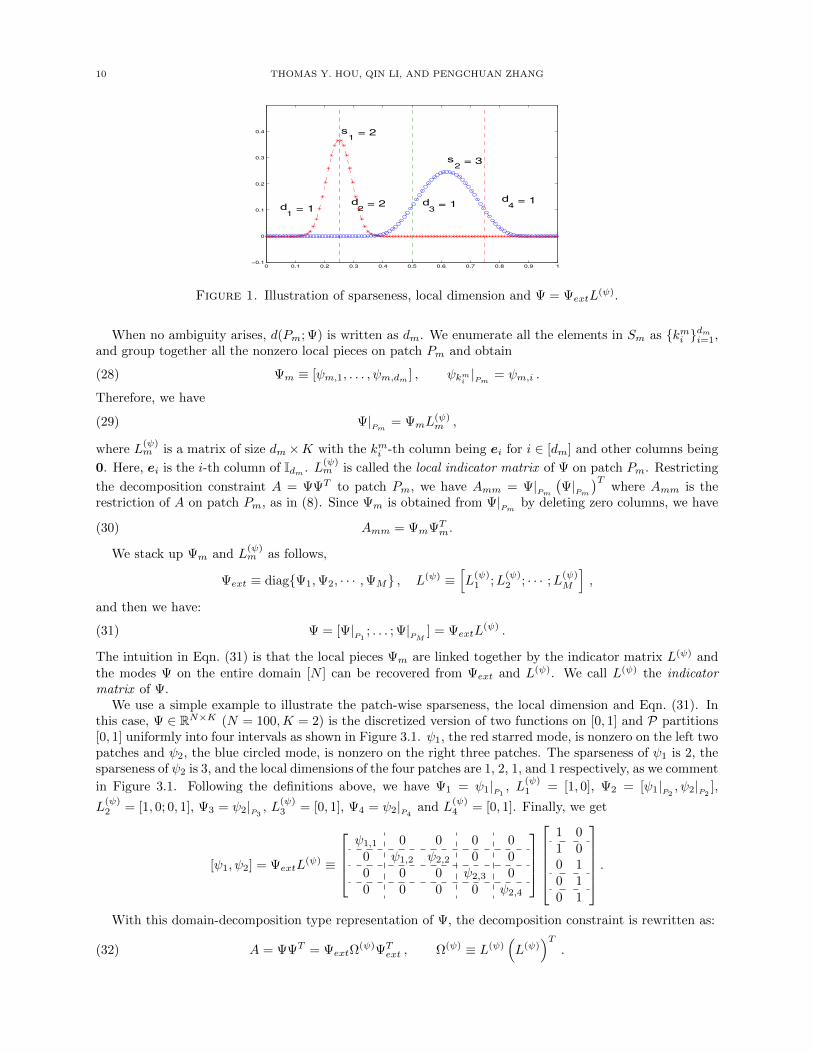
Figure 1. Illustration of sparseness, local dimension and Ψ = ΨextL(ψ).
When no ambiguity arises, d(Pm; Ψ) is written as dm. We enumerate all the elements in Sm as kmi dmi=1,
and group together all the nonzero local pieces on patch Pm and obtain
(28) Ψm ≡ [ψm,1, . . . , ψm,dm ] , ψkmi |Pm= ψm,i .
Therefore, we have
(29) Ψ|Pm
= ΨmL(ψ)m ,
where L(ψ)m is a matrix of size dm×K with the kmi -th column being ei for i ∈ [dm] and other columns being
0. Here, ei is the i-th column of Idm . L(ψ)m is called the local indicator matrix of Ψ on patch Pm. Restricting
the decomposition constraint A = ΨΨT to patch Pm, we have Amm = Ψ|Pm
(Ψ|
Pm
)Twhere Amm is the
restriction of A on patch Pm, as in (8). Since Ψm is obtained from Ψ|Pm
by deleting zero columns, we have
(30) Amm = ΨmΨTm.
We stack up Ψm and L(ψ)m as follows,
Ψext ≡ diagΨ1,Ψ2, · · · ,ΨM , L(ψ) ≡[L(ψ)1 ;L
(ψ)2 ; · · · ;L
(ψ)M
],
and then we have:
(31) Ψ = [Ψ|P1
; . . . ; Ψ|PM
] = ΨextL(ψ) .
The intuition in Eqn. (31) is that the local pieces Ψm are linked together by the indicator matrix L(ψ) andthe modes Ψ on the entire domain [N ] can be recovered from Ψext and L(ψ). We call L(ψ) the indicatormatrix of Ψ.
We use a simple example to illustrate the patch-wise sparseness, the local dimension and Eqn. (31). Inthis case, Ψ ∈ RN×K (N = 100,K = 2) is the discretized version of two functions on [0, 1] and P partitions[0, 1] uniformly into four intervals as shown in Figure 3.1. ψ1, the red starred mode, is nonzero on the left twopatches and ψ2, the blue circled mode, is nonzero on the right three patches. The sparseness of ψ1 is 2, thesparseness of ψ2 is 3, and the local dimensions of the four patches are 1, 2, 1, and 1 respectively, as we comment
in Figure 3.1. Following the definitions above, we have Ψ1 = ψ1|P1, L
(ψ)1 = [1, 0], Ψ2 = [ψ1|P2
, ψ2|P2],
L(ψ)2 = [1, 0; 0, 1], Ψ3 = ψ2|P3
, L(ψ)3 = [0, 1], Ψ4 = ψ2|P4
and L(ψ)4 = [0, 1]. Finally, we get
[ψ1, ψ2] = ΨextL(ψ) ≡
ψ1,1 0 0 0 0
0 ψ1,2 ψ2,2 0 00 0 0 ψ2,3 00 0 0 0 ψ2,4
1 01 00 10 10 1
.With this domain-decomposition type representation of Ψ, the decomposition constraint is rewritten as:
(32) A = ΨΨT = ΨextΩ(ψ)ΨT
ext , Ω(ψ) ≡ L(ψ)(L(ψ)
)T.

A SPARSE DECOMPOSITION OF LOW RANK SYMMETRIC POSITIVE SEMI-DEFINITE MATRICES 11
Here, Ω(ψ) has a role similar to that of Ω in the ISMD. It can be viewed as the correlation matrix of A underbasis Ψext, just like how Λ and Ω are defined.
Finally, we provide two useful properties of the local indicator matrices L(ψ)m , which are direct consequences
of their definitions. Its proof is elementary and can be found in Appendix A.
Proposition 3.1. For an arbitrary decomposition A = ΨΨT ,
(1) The k-th column of L(ψ), denoted as l(ψ)k , satisfies ‖l(ψ)k ‖1 = sk where sk is the patch-wise sparseness
of ψk, as in Definition 1.1. Moreover, different columns in L(ψ) have disjoint supports.(2) Define
(33) B(ψ)n;m ≡ Ω(ψ)
mn
(Ω(ψ)mn
)T,
where Ω(ψ)mn ≡ L
(ψ)m (L
(ψ)n )T is the (m,n)-th block of Ω(ψ). B
(ψ)n;m is diagonal with diagonal entries
either 1 or 0. Moreover, B(ψ)n;m(i, i) = 1 if and only if there exists k ∈ [K] such that ψk|Pm
= ψm,iand ψk|Pn
6= 0.
Since different columns in L(ψ) have disjoint supports, Ω(ψ) ≡ L(ψ)(L(ψ)
)Thas a block-diagonal structure
with K blocks. The k-th diagonal block is the one contributed by l(ψ)k
(l(ψ)k
)T. Therefore, as long as we
obtain Ω(ψ), we can use the pivoted Cholesky decomposition to efficiently recover L(ψ). The ISMD followsthis rationale: we first construct local pieces Ψext ≡ diagΨ1,Ψ2, · · · ,ΨM for certain set of intrinsic sparsemodes Ψ; then from the decomposition constraint (32) we are able to compute Ω(ψ); finally, the pivotedCholesky decomposition is applied to obtain L(ψ) and the modes are assembled by Ψ = ΨextL
(ψ). Obviously,the key step is to construct Ψext, which are local pieces of a set of intrinsic sparse modes – this is exactlywhere the regular-sparse property and the joint diagonalization come into play.
3.2. regular-sparse property and local modes construction. In this and the next subsections (Sec-tion 3.2 - Section 3.3), we assume that the submatrices Amm are well conditioned and thus the exact localeigen decomposition (9) is used in the ISMD.
Combining the local eigen decomposition (9) and local decomposition constraint (30), there exists D(ψ)m ∈
RKm×dm such that
(34) Ψm = HmD(ψ)m .
Moreover, since the local eigenvectors are linearly independent, we have
(35) dm ≥ Km , D(ψ)m
(D(ψ)m
)T= IKm
.
We see that dm = Km if and only if columns in Ψm is also linearly independent. In this case, D(ψ)m is unitary,
i.e., D(ψ)m ∈ O(Km). This is exactly what is required by the regular-sparse property, see Definition 1.2. It is
easy to see that we have the following equivalent definitions of regular-sparse property.
Proposition 3.2. The following assertions are equivalent.
(1) The partition P is regular-sparse with respect to A.
(2) There exists a decomposition A =∑Kk=1 ψkψ
Tk such that on every patch Pm its local dimension dm
is equal to the local rank Km, i.e., dm = Km.
(3) The minimum of problem (3) is∑Mm=1Km.
The proof is elementary and is omitted here. By Proposition 3.2, for regular-sparse partitions local pieces
of a set of intrinsic sparse modes can be constructed from rotating local eigenvectors, i.e., Ψm = HmD(ψ)m .
All the local rotations D(ψ)m Mm=1 are coupled by the decomposition constraint A = ΨΨT . At first glance,
it seems impossible to find such Dm from this big coupled system. However, the following lemma gives a
necessary condition that D(ψ)m must satisfy so that HmD
(ψ)m are local pieces of a set of intrinsic sparse modes.
More importantly, this necessary condition turns out to be sufficient, and thus provides us a criterion to findthe local rotations.
12 THOMAS Y. HOU, QIN LI, AND PENGCHUAN ZHANG
Lemma 3.1. Suppose that P is regular-sparse w.r.t. A and that ψkKk=1 is an arbitrary set of intrinsic
sparse modes. Denote the transformation from Hm to Ψm as D(ψ)m , i.e., Ψm = HmD
(ψ)m . Then D
(ψ)m is
unitary and jointly diagonalizes Σn;mMn=1, which are defined in (14). Specifically, we have
(36) B(ψ)n;m =
(D(ψ)m
)TΣn;mD
(ψ)m , m = 1, 2, . . . ,M,
where B(ψ)n;m ≡ Ω
(ψ)mn
(Ω
(ψ)mn
)T, defined in (33), is diagonal with diagonal entries either 0 or 1.
Proof. From item 3 in Proposition 3.2, any set of intrinsic sparse modes must have local dimension dm =
Km on patch Pm. Therefore, the transformation D(ψ)m from Hm to Ψm must be unitary. Combining
Ψm = HmD(ψ)m with the decomposition constraint (32), we get
A = HextD(ψ)Ω(ψ)
(D(ψ)
)THext,
where D(ψ) = diagD(ψ)1 , D
(ψ)2 , . . . , D
(ψ)M . Recall that A = HextΛHext and that Hext has linearly indepen-
dent columns, we obtain
(37) Λ = D(ψ)Ω(ψ)(D(ψ)
)T,
or block-wisely,
(38) Λmn = D(ψ)m Ω(ψ)
mn
(D(ψ)n
)T.
Since D(ψ)n is unitary, Eqn. (36) naturally follows the definitions of B
(ψ)n;m and Σn;m. By item 2 in Proposi-
tion 3.1, we know that B(ψ)n;m is diagonal with diagonal entries either 0 or 1.
Lemma 3.1 guarantees that D(ψ)m for an arbitrary set of intrinsic sparse modes is the minimizer of the joint
diagonalization problem (13). In the other direction, the following lemma guarantees that any minimizer ofthe joint diagonalization problem (13), denoted as Dm, transforms local eigenvectors Hm to Gm, which arethe local pieces of certain intrinsic sparse modes.
Lemma 3.2. Suppose that P is regular-sparse w.r.t. A and that Dm is a minimizer of the joint diagonaliza-tion problem (13). As in the ISMD, define Gm = HmDm. Then there exists a set of intrinsic sparse modessuch that its local pieces on patch Pm are equal to Gm.
Before we prove this lemma, we examine the uniqueness property of intrinsic sparse modes. It is easy tosee that permutations and sign flips of a set of intrinsic sparse modes are still a set of intrinsic sparse modes.Specifically, if ψkKk=1 is a set of intrinsic sparse modes and σ : [K] → [K] is a permutation, ±ψσ(k)Kk=1
is another set of intrinsic sparse modes. Another kind of non-uniqueness comes from the following concept– identifiability.
Definition 3.2 (Identifiability). For two modes g1, g2 ∈ RN , they are unidentifiable on partition P if theyare supported on the same patches, i.e., P ∈ P : g1|P 6= 0 = P ∈ P : g2|P 6= 0. Otherwise, theyare identifiable. For a collection of modes giki=1 ⊂ RN , they are unidentifiable iff any pair of them areunidentifiable. They are pair-wisely identifiable iff any pair of them are identifiable.
It is important to point out that the identifiability above is based on the resolution of partition P.Unidentifiable modes for partition P may have different supports and become identifiable on a refinedpartition. Unidentifiable intrinsic sparse modes lead to another kind of non-uniqueness for intrinsic sparsemodes. For instance, when two intrinsic sparse modes ψm and ψn are unidentifiable, then any rotation of[ψm, ψn] while keeping other intrinsic sparse modes unchanged is still a set of intrinsic sparse modes.
Local pieces of intrinsic sparse modes inherit this kind of non-uniqueness. Suppose Ψm ≡ [ψm,1, . . . , ψm,dm ]are the local pieces of a set of intrinsic sparse modes Ψ on patch Pm. First, if σ : [dm]→ [dm] is a permutation,
±ψm,σ(i)dmi=1 are local pieces of another set of intrinsic sparse modes. Second, if ψm,i and ψm,j are the localpieces of two unidentifiable intrinsic sparse modes, then any rotation of [ψm,i, ψm,j ] while keeping other localpieces unchanged are local pieces of another set of intrinsic sparse modes. It turns out that this kind of non-uniqueness has a one-to-one correspondence with the non-uniqueness of joint diagonalizers for problem (13),
A SPARSE DECOMPOSITION OF LOW RANK SYMMETRIC POSITIVE SEMI-DEFINITE MATRICES 13
which is characterized in Theorem C.1. Keeping this correspondence in mind, the proof of Lemma 3.2 isquite intuitive.
Proof. [Proof of Lemma 3.2] Let Ψ ≡ [ψ1, . . . , ψK ] be an arbitrary set of intrinsic sparse modes. We ordercolumns in Ψ such that unidentifiable modes are grouped together, denoted as Ψ = [Ψ1, . . . ,ΨQ], where Qis the number of unidentifiable groups. Accordingly on patch Pm, Ψm = [Ψm,1, . . . ,Ψm,Qm
] where Qm is thenumber of nonzero unidentifiable groups. Denote the number of columns in each group as nm,i, i.e., thereare nm,i modes in ψkKk=1 that are nonzero and unidentifiable on patch Pm.
Making use of item 2 in Proposition 3.1, one can check that ψm,i and ψm,j are unidentifiable if and only
if B(ψ)n;m(i, i) = B
(ψ)n;m(j, j) for all n ∈ [M ]. Since unidentifiable pieces in Ψm are grouped together, the same
diagonal entries in B(ψ)n;mMn=1 are grouped together as required in Theorem C.1. Now we apply Theorem C.1
with Mk replaced by Σn;m, Λk replaced by B(ψ)n;m, D replaced by D
(ψ)m , the number of distinct eigenvalues
m replaced by Qm, eigenvalue’s multiplicity qi replaced by nm,i and the diagonalizer V replaced by Dm.Therefore, there exists a permutation matrix Πm and a block diagonal matrix Vm such that
(39) DmΠm = D(ψ)m Vm , Vm = diagVm,1, . . . , Vm,Qm .
Recall that Gm = HmDm and Ψm = HmD(ψ)m , we obtain that
(40) GmΠm = ΨmVm = [Ψm,1Vm,1 , . . . ,Ψm,QmVm,Qm ] .
From Eqn. (40), we can see that identifiable pieces are completely separated and the small rotation matrices,Vm,i, only mix unidentifiable pieces Ψm,i. Πm merely permutes the columns in Gm. From the non-uniquenessof local pieces of intrinsic sparse modes, we conclude that Gm are local pieces of another set of intrinsic sparsemodes.
We point out that the local pieces GmMm=1 constructed by the ISMD on different patches may correspondto different sets of intrinsic sparse modes. Therefore, the final “patch-up” step should further modify andconnect them to build a set of intrinsic sparse modes. Fortunately, the pivoted Cholesky decompositionelegantly solves this problem.
3.3. Optimal sparse recovery and consistency of the ISMD. As defined in the ISMD, Ω is the cor-relation matrix of A with basis Gext, see (15). If Ω enjoys a block diagonal structure with each block
corresponding to a single intrinsic sparse mode, just like Ω(ψ) ≡ L(ψ)(L(ψ)
)T, the pivoted Cholesky decom-
position can be utilized to recover the intrinsic sparse modes.It is fairly easy to see that Ω indeed enjoys such a block diagonal structure when there is one set of intrinsic
sparse modes that are pair-wisely identifiable. Denoting this identifiable set as ψkKk=1 (only its existenceis needed), by Eqn. (39), we know that on patch Pm there is a permutation matrix Πm and a diagonal
matrix Vm with diagonal entries either 1 or -1 such that DmΠm = D(ψ)m Vm. Recall that Λ = DΩDT =
D(ψ)Ω(ψ)(D(ψ)
)T, see (16) and (38), we have
(41) Ω = DTD(ψ)Ω(ψ)(D(ψ)
)TD = ΠV TΩ(ψ)VΠT ,
in which V = diagV1, . . . , Vm is diagonal with diagonal entries either 1 or -1 and Π = diagΠ1, . . . ,Πm isa permutation matrix. Since the action of ΠV T does not change the block diagonal structure of Ω(ψ), Ω stillhas such a structure and the pivoted Cholesky decomposition can be readily applied. In fact, the action ofΠV T exactly corresponds to the column permutation and sign flips of intrinsic sparse modes, which is theonly kind of non-uniqueness of problem (3) when the intrinsic sparse modes are pair-wisely identifiable. Forthe general case when there are unidentifiable intrinsic sparse modes, Ω still has the block diagonal structurewith each block corresponding to a group of unidentifiable modes, resulting in the following theorem.
Theorem 3.1. Suppose the domain partition P is regular-sparse with respect to A. Let A = GGT be thedecomposition given by the ISMD (19) and Ψ ≡ [ψ1, . . . , ψK ] be an arbitrary set of intrinsic sparse modes. Letcolumns in Ψ be ordered such that unidentifiable modes are grouped together, denoted as Ψ = [Ψ1, . . . ,ΨQ],where Q is the number of unidentifiable groups and nq is the number of modes in Ψq. Then there exists Qrotation matrices Uq ∈ Rnq×nq (1 ≤ q ≤ Q) such that
(42) G = [Ψ1U1, . . . ,ΨQUQ],

14 THOMAS Y. HOU, QIN LI, AND PENGCHUAN ZHANG
with reordering of columns in G if necessary. It immediately follows that
• the ISMD generates one set of intrinsic sparse modes.• the intrinsic sparse modes are unique up to permutations and rotations within unidentifiable modes.
Proof. By Eqn. (39), Eqn. (41) still holds true with block diagonal Vm for m ∈ [M ]. Without loss ofgenerality, we assume that Π = I since permutation does not change the block diagonal structure that wedesire. Then from Eqn. (41) we have
(43) Ω = V TΩ(ψ)V = V TL(ψ)(L(ψ)
)TV.
In terms of block-wise formulation, we get
(44) Ωmn = V TmΩ(ψ)mnVn = V TmL
(ψ)m
(L(ψ)n
)TVn.
Correspondingly, by (40) the local pieces satisfy
Gm = [Gm,1 , . . . , Gm,Qm] = [Ψm,1Vm,1 , . . . ,Ψm,Qm
Vm,Qm] .
Now, we prove that Ω has the block diagonal structure in which each block corresponds to a group ofunidentifiable modes. Specifically, Gm,i = Ψm,iVm,i and Gn,j = Ψn,jVn,j are two identifiable groups, i.e.,Ψm,i and Ψn,j are from two identifiable groups, and we want to prove that the corresponding block in Ω,
denoted as Ωm,i;n,j , is zero. From Eqn. (44), one gets Ωm,i;n,j = V Tm,iL(ψ)m,i
(L(ψ)n,j
)TVn,j , where L
(ψ)m,i are the
rows in L(ψ)m corresponding to Ψm,i. L
(ψ)n,j is defined similarly. Due to identifiability between Ψm,i and Ψn,j ,
we know L(ψ)m,i
(L(ψ)n,j
)T= 0 and thus we obtain the block diagonal structure of Ω.
In (18), the ISMD performs the pivoted Cholesky decomposition Ω = PLLTPT and generates sparsemodes G = GextPL. Due to the block diagonal structure in Ω, every column in PL can only have nonzeroentries on local pieces that are not identifiable. Therefore, columns in G have identifiable intrinsic sparsemodes completely separated and unidentifiable intrinsic sparse modes rotated (including sign flip) by certainunitary matrices. Therefore, G is a set of intrinsic sparse modes.
Due to the arbitrary choice of Ψ, we know that the intrinsic sparse modes are unique to permutationsand rotations within unidentifiable modes.
Remark 3.1. From the proof above, we can see that it is the block diagonal structure of Ω that leads to therecovery of intrinsic sparse modes. The pivoted Cholesky decomposition is one way to explore this structure.In fact, the pivoted Cholesky decomposition can be replaced by any other matrix decomposition that preservesthis block diagonal structure, for instance, the eigen decomposition if there is no degeneracy.
Despite the fact that the intrinsic sparse modes depend on the partition P, the following theorem guar-antees that the solutions to problem (3) give consistent results as long as the partition is regular-sparse.
Theorem 3.2. Suppose that Pc is a partition, Pf is a refinement of Pc and that Pf is regular-sparse.
Suppose g(c)k Kk=1 and g(f)k Kk=1 (with reordering if necessary) are the intrinsic sparse modes produced by
the ISMD on Pc and Pf , respectively. Then for every k ∈ 1, 2, . . . ,K, in the coarse partition Pc g(c)kand g
(f)k are supported on the same patches, while in the fine partition Pf the support patches of g
(f)k are
contained in the support patches of g(c)k , i.e.,
P ∈ Pc : g(f)k |P 6= 0 = P ∈ Pc : g
(c)k |P 6= 0,
P ∈ Pf : g(f)k |P 6= 0 ⊂ P ∈ Pf : g
(c)k |P 6= 0.
Moreover, if g(c)k is identifiable on the coarse patch Pc, it remains unchanged when the ISMD is performed
on the refined partition Pf , i.e., g(f)k = ±g(c)k .
Proof. Given the finer partition Pf is regular-sparse, it is easy to prove the coarser partition Pc is also regular-sparse.2 Notice that if two modes are identifiable on the coarse partition Pc, they must be identifiable on the
2We provide the proof in supplementary materials, see Lemma B.1.

A SPARSE DECOMPOSITION OF LOW RANK SYMMETRIC POSITIVE SEMI-DEFINITE MATRICES 15
fine partition Pf . However, the other direction is not true, i.e., unidentifiable modes may become identifiableif the partition is refined. Based on this observation, Theorem 3.2 is a simple corollary of Theorem 3.1.
Finally, we provide a necessary condition for a partition to be regular-sparse as follows.
Proposition 3.3. If P is regular-sparse w.r.t. A, all eigenvalues of Λ are integers. Here, Λ is computed inthe ISMD by Eqn. (12).
Proof. Let ψkKk=1 be a set of intrinsic sparse modes. Since P is regular-sparse, D(ψ) in Eqn. (37) is unitary.
Therefore, Λ and Ω(ψ) ≡ L(ψ)(L(ψ)
)Tshare the same eigenvalues. Due to the block-diagonal structure of
Ω(ψ), one can see that
Ω(ψ) ≡ L(ψ)(L(ψ)
)T=
K∑k=1
l(ψ)k
(l(ψ)k
)Tis in fact the eigen decomposition of Ω(ψ). The eigenvalue corresponding to the eigenvector l
(ψ)k is ‖l(ψ)k ‖22,
which is also equal to ‖l(ψ)k ‖1 because L(ψ) only elements 0 or 1. From item 1 in Proposition 3.1, ‖l(ψ)k ‖1 = sk,which is the patch-wise sparseness of ψk.
Combining Theorem 3.1, Theorem 3.2 and Proposition 3.3, we can develop a hierarchical process thatgradually finds the finest regular-sparse partition and thus obtains the sparsest decomposition using theISMD. This sparsest decomposition can be viewed as another definition of intrinsic sparse modes, which areindependent of partitions. In our numerical examples, our partitions are all uniform but with different patchsizes. We see that even when the partition is not regular-sparse, the ISMD still produces a nearly optimalsparse decomposition.
4. Perturbation analysis and two modifications
In real applications, data are often contaminated by noises. For example, when measuring the covariancefunction of a random field, sample noise is inevitable if a Monte Carlo type sampling method is utilized.A basic requirement for a numerical algorithm is its stability with respect to small noises. In Section 4.1,under several assumptions, we are able to prove that the ISMD is stable with respect to small perturbationsin the input A. In Section 4.2, we provide two modified ISMD algorithms that effectively handle noises indifferent situations.
4.1. Perturbation analysis of the ISMD. We consider the additive perturbation here, i.e., A is anapproximately low rank symmetric PSD matrix that satisfies
(45) A = A+ εA, ‖A‖2 ≤ 1.
Here, A is the noiseless rank-K symmetric PSD matrix and A is the symmetric additive perturbation and
ε > 0 quantifies the noise level. We divide A into blocks that are conformal with blocks of A in (8) and thus
Amn = Amn + εAmn. In this case, we need to apply the truncated local eigen decomposition (10) to capture
the correct local rank Km. Suppose the eigen decomposition of Amm is
Amm =
Km∑i=1
γm,ihn,ihTn,i +
∑i>Km
γm,ihn,ihTn,i.
In this subsection, we assume that the noise level is very small with ε 1 such that there is an energy gapbetween γm,Km
and γm,Km+1. Therefore, the truncation (10) captures the correct local rank Km, i.e.,
(46) Amm ≈ A(t)mm ≡
Km∑i=1
γm,ihn,ihTn,i ≡ HmH
Tm.
In the rest of the ISMD, the perturbed local eigenvectors Hm is used as Hm in the noiseless case. We expectthat our ISMD is stable with respect to this small perturbation and generates slightly perturbed intrinsicsparse modes of A.
To carry out this perturbation analysis, we will restrict ourselves to the case when intrinsic sparse modesof A are pair-wisely identifiable and thus it is possible to compare the error between the noisy output gkwith A’s intrinsic sparse mode gk. When there are unidentifiable intrinsic sparse modes of A, it only makes

16 THOMAS Y. HOU, QIN LI, AND PENGCHUAN ZHANG
sense to consider the perturbation of the subspace spanned by those unidentifiable modes and we will notconsider this case in this paper. The following lemma is a preliminary result on the perturbation analysis oflocal pieces Gm.
Lemma 4.1. Suppose that partition P is regular-sparse with respect to A and all intrinsic modes are iden-
tifiable with each other. Furthermore, we assume that for all m ∈ [M ] there exists E(eig)m such that
(47) A(t)mm = (I + εE(eig)
m )Amm
(I + ε(E(eig)
m )T)
and ‖E(eig)m ‖2 ≤ Ceig.
Here Ceig is a constant depending on A but not on ε or A. Then there exists E(jd)m ∈ RKm×Km such that
(48) Gm = (I + εE(eig)m )Gm(I + εE(jd)
m +O(ε2))Jm and ‖E(jd)m ‖F ≤ Cjd,
where Gm and Gm are local pieces constructed by the ISMD with input A and A respectively, Jm is theproduct of a permutation matrix with a diagonal matrix having only ±1 on its diagonal, and Cjd is a constant
depending on A but not on ε or A. Here, ‖ • ‖2 and ‖ • ‖F are matrix spectral norm and Frobenius norm,respectively.
Lemma 4.1 ensures that local pieces of intrinsic sparse modes can be constructed with O(ε) accuracy upto permutation and sign flips (characterized by Jm in (48)) under several assumptions. The identifiabilityassumption is necessary. Without such assumption, these local pieces are not uniquely determined upto permutations and sign flips. The assumption (47) holds true when eigen decomposition of Amm iswell conditioned, i.e., both eigenvalues and eigenvectors are well conditioned. We expect that a strongerperturbation result is still true without making this assumption. The proof of Lemma 4.1 is an applicationof perturbation analysis for the joint diagonalization problem [5], and is presented in Appendix D.
Finally, Ω is the correlation matrix of A with basis Gext = diagG1, G2, . . . , GM. Specifically, the
(m,n)-th block of Ω is given by
Ωmn = G†mAmn
(G†n
)T.
Without loss of generality, we can assume that Jm = IKmin (48).3 Based on the perturbation analysis of
Gm in Lemma 4.1 and the standard perturbation analysis of pseudo-inverse, for instance see Theorem 3.4
in [39], it is straightforward to get a bound of the perturbations in Ω, i.e.,
(49) ‖Ω− Ω‖2 ≤ Cismdε.
Here, Cismd depends on the smallest singular value of Gm and the constants Ceig and Cjd in Lemma 4.1.Notice that when all intrinsic modes are identifiable with each other, the entries of Ω are either 0 or ±1.
Therefore, when Cismdε is small enough, we can exactly recover Ω from Ω as below:
(50) Ωij =
−1, for Ωij < −0.5,
0, for Ωij ∈ [−0.5, 0.5],
1, for Ωij > 0.5.
Following Algorithm 1, we get the pivoted Cholesky decomposition Ω = PLLTPT and output the perturbedintrinsic sparse modes
G = GextPL.
Notice that the patch-wise sparseness information is all coded in L and we can reconstruct L exactly due to
the thresholding step (50), G has the same patch-wise sparse structure as G. Moreover, because the local
pieces Gext are constructed with O(ε) error, we have
(51) ‖G−G‖2 ≤ Cgε,
where the constant Cg only depends the constants Ceig and Cjd in Lemma 4.1.
3One can check that JmMm=1 only affect the sign of recovered intrinsic sparse modes [g1, g2, . . . , gK ] if pivoted Cholesky
decomposition is applied on Ω.

A SPARSE DECOMPOSITION OF LOW RANK SYMMETRIC POSITIVE SEMI-DEFINITE MATRICES 17
4.2. Two modified ISMD algorithms. In Section 4.1, we have shown that the ISMD is robust to smallnoises under the assumption of regular sparsity and identifiability. In this section, we provide two modifiedversions of the ISMD to deal with the cases when these two assumptions fail. The first modification aims
at constructing intrinsic sparse modes from noisy input A in the small noise region, as in Section (4.1), butit does not require the regular sparsity and identifiability. The second modification aims at constructing a
simultaneous low-rank and sparse approximation of A when the noise is big. Our numerical experimentsdemonstrate that these modified algorithms are quite effective in practice.
4.2.1. ISMD with thresholding. In the general case when unidentifiable pairs of intrinsic sparse modes exist,the thresholding idea (50) is still applicable but the threshold εth should be learnt from the data, i.e., the
entries in Ω. Specifically, there are O(1) entries in Ω corresponding to the slightly perturbed nonzero entries
in Ω; there are also many O(ε) entries that are contributed by the noise εA. If the noise level ε is small enough,we can see a gap between these two group of entries, and a threshold εth is chosen such that it separates thesetwo groups. A simple 2-cluster algorithm is able to identify the threshold εth. In our numerical examples we
draw the histogram of absolute values of entries in Ω and it clearly shows the 2-cluster effect, see Figure 10.
Finally, we set all the entries in Ω with absolute value less than εth to 0. In this approach we do not need toknow the noise level ε a priori and we just learn the threshold from the data. To modify Algorithm 1 withthis thresholding technique, we just need to add one line between assembling Ω (Line 15) and the pivotedCholesky decomposition (Line 16), see Algorithm 2.
Algorithm 2 Intrinsic sparse mode decomposition with thresholding
Require: A ∈ RN×N : symmetric and PSD; P = PmMm=1: partition of index set [N ]Ensure: G = [g1, g2, · · · , gK ]: A ≈ GGT
1: The same with Algorithm 1 from Line 1 to Line 132: . Assemble Ω, thresholding and its pivoted Cholesky decomposition3: Ω = DTΛD4: Learn a threshold εth from Ω and set all the entries in Ω with absolute value less than εth to 05: Ω = PLLTPT
6: . Assemble the intrinsic sparse modes G7: G = HextDPL
It is important to point out that when the noise is large, the O(1) entries and O(ε) entries mix together.In this case, we cannot identify such a threshold εth to separate them, and the assumption that there isan energy gap between γm,Km and γm,Km+1 is invalid. In the next subsection, we will present the secondmodified version to overcome this difficulty.
4.2.2. Low rank approximation with ISMD. In the case when there is no gap between γm,Km and γm,Km+1
(i.e., no well-defined local ranks), or when the noise is so large that the threshold εth cannot be identified, wemodify our ISMD to give a low-rank approximation of A ≈ GGT , in which G is observed to be patch-wisesparse from our numerical examples.
In this modification, the normalization (17) is applied and thus we have:
A ≈ GextΩGText.It is important to point out that Ω has the same block diagonal structure as Ω but has different eigenvalues.Specifically, for the case when there is no noise and the regular-sparse assumption holds true, Ω has eigen-values ‖gk‖22Kk=1 for a certain set of intrinsic sparse modes gk, while Ω has eigenvalues skKk=1 (here sk isthe patch-wise sparseness of the intrinsic sparse mode). We first perform eigen decomposition Ω = LLT andthen assemble the final result by G = GextL. The modified algorithm is summarized in Algorithm 3.
Here we replace the pivoted Cholesky decomposition of Ω in Algorithm 1 by eigen decomposition of Ω.From Remark 3.1, this modified version generates exactly the same result with Algorithm 1 if all the intrinsicsparse modes have different l2 norm (there are no repeated eigenvalues in Ω). The advantage of the pivotedCholesky decomposition is its low computational cost and the fact that it always exploits the (unordered)block diagonal structure of Ω. However, it is more sensitive to noise compared to eigen decomposition.In contrast, eigen decomposition is much more robust to noise. Moreover, eigen decomposition gives the
18 THOMAS Y. HOU, QIN LI, AND PENGCHUAN ZHANG
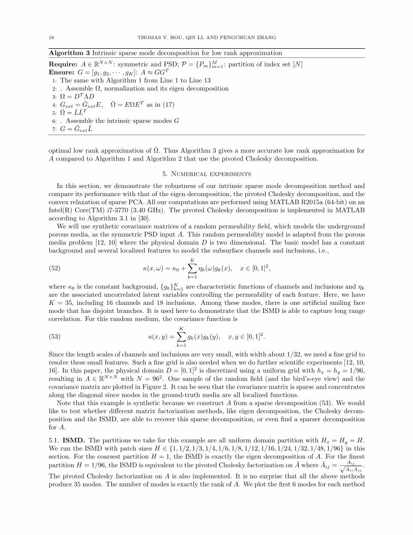
Algorithm 3 Intrinsic sparse mode decomposition for low rank approximation
Require: A ∈ RN×N : symmetric and PSD; P = PmMm=1: partition of index set [N ]Ensure: G = [g1, g2, · · · , gK ]: A ≈ GGT
1: The same with Algorithm 1 from Line 1 to Line 132: . Assemble Ω, normalization and its eigen decomposition3: Ω = DTΛD4: Gext = GextE, Ω = EΩET as in (17)5: Ω = LLT
6: . Assemble the intrinsic sparse modes G7: G = GextL
optimal low rank approximation of Ω. Thus Algorithm 3 gives a more accurate low rank approximation forA compared to Algorithm 1 and Algorithm 2 that use the pivoted Cholesky decomposition.
5. Numerical experiments
In this section, we demonstrate the robustness of our intrinsic sparse mode decomposition method andcompare its performance with that of the eigen decomposition, the pivoted Cholesky decomposition, and theconvex relaxation of sparse PCA. All our computations are performed using MATLAB R2015a (64-bit) on anIntel(R) Core(TM) i7-3770 (3.40 GHz). The pivoted Cholesky decomposition is implemented in MATLABaccording to Algorithm 3.1 in [30].
We will use synthetic covariance matrices of a random permeability field, which models the undergroundporous media, as the symmetric PSD input A. This random permeability model is adapted from the porousmedia problem [12, 10] where the physical domain D is two dimensional. The basic model has a constantbackground and several localized features to model the subsurface channels and inclusions, i.e.,
(52) κ(x, ω) = κ0 +
K∑k=1
ηk(ω)gk(x), x ∈ [0, 1]2,
where κ0 is the constant background, gkKk=1 are characteristic functions of channels and inclusions and ηkare the associated uncorrelated latent variables controlling the permeability of each feature. Here, we haveK = 35, including 16 channels and 18 inclusions. Among these modes, there is one artificial smiling facemode that has disjoint branches. It is used here to demonstrate that the ISMD is able to capture long rangecorrelation. For this random medium, the covariance function is
(53) a(x, y) =
K∑k=1
gk(x)gk(y), x, y ∈ [0, 1]2.
Since the length scales of channels and inclusions are very small, with width about 1/32, we need a fine grid toresolve these small features. Such a fine grid is also needed when we do further scientific experiments [12, 10,16]. In this paper, the physical domain D = [0, 1]2 is discretized using a uniform grid with hx = hy = 1/96,resulting in A ∈ RN×N with N = 962. One sample of the random field (and the bird’s-eye view) and thecovariance matrix are plotted in Figure 2. It can be seen that the covariance matrix is sparse and concentratesalong the diagonal since modes in the ground-truth media are all localized functions.
Note that this example is synthetic because we construct A from a sparse decomposition (53). We wouldlike to test whether different matrix factorization methods, like eigen decomposition, the Cholesky decom-position and the ISMD, are able to recover this sparse decomposition, or even find a sparser decompositionfor A.
5.1. ISMD. The partitions we take for this example are all uniform domain partition with Hx = Hy = H.We run the ISMD with patch sizes H ∈ 1, 1/2, 1/3, 1/4, 1/6, 1/8, 1/12, 1/16, 1/24, 1/32, 1/48, 1/96 in thissection. For the coarsest partition H = 1, the ISMD is exactly the eigen decomposition of A. For the finest
partition H = 1/96, the ISMD is equivalent to the pivoted Cholesky factorization on A where Aij =Aij√AiiAjj
.
The pivoted Cholesky factorization on A is also implemented. It is no surprise that all the above methodsproduce 35 modes. The number of modes is exactly the rank of A. We plot the first 6 modes for each method

A SPARSE DECOMPOSITION OF LOW RANK SYMMETRIC POSITIVE SEMI-DEFINITE MATRICES 19
0
0.5
1
0
0.5
10
20
40
60
fieldSample fieldSample
0 0.2 0.4 0.6 0.8 10
0.2
0.4
0.6
0.8
1
Figure 2. One sample and the bird’s-eye view. The covariance matrix is plotted on the right.
ISMD: H=1/1 ISMD: H=1/1 ISMD: H=1/1 ISMD: H=1/1 ISMD: H=1/1 ISMD: H=1/1
ISMD: H=1/8 ISMD: H=1/8 ISMD: H=1/8 ISMD: H=1/8 ISMD: H=1/8 ISMD: H=1/8
ISMD: H=1/32 ISMD: H=1/32 ISMD: H=1/32 ISMD: H=1/32 ISMD: H=1/32 ISMD: H=1/32
Pivoted Cholesky
0 0.2 0.4 0.6 0.8 10
0.2
0.4
0.6
0.8
1Pivoted Cholesky
0 0.2 0.4 0.6 0.8 10
0.2
0.4
0.6
0.8
1Pivoted Cholesky
0 0.2 0.4 0.6 0.8 10
0.2
0.4
0.6
0.8
1Pivoted Cholesky
0 0.2 0.4 0.6 0.8 10
0.2
0.4
0.6
0.8
1Pivoted Cholesky
0 0.2 0.4 0.6 0.8 10
0.2
0.4
0.6
0.8
1Pivoted Cholesky
0 0.2 0.4 0.6 0.8 10
0.2
0.4
0.6
0.8
1
Figure 3. First 6 eigenvectors (H=1); First 6 intrinsic sparse modes (H=1/8, regular-sparse); First 6 intrinsic sparse modes (H=1/32; not regular-sparse); First 6 modes from thepivoted Cholesky decomposition of A
in Figure 3. We can see that both the eigen decomposition (ISMD with H = 1) and the pivoted Choleskyfactorization on A generate modes which mix different localized feathers together. On the other hand, theISMD with H = 1/8 and H = 1/32 exactly recover the localized feathers, including the smiling face.

20 THOMAS Y. HOU, QIN LI, AND PENGCHUAN ZHANG
0 5 10 15 20 25 30 35
0
5
10
15
20
25
Eigenvalues of Correlation Matrix Λ
H=1
H=1/8
H=1/32
subdomain size: H
1/96 1/48 1/32 1/24 1/16 1/12 1/8 1/6 1/4 1/3 1/2 1
CP
U T
ime
100
101
102
103
Comparison of CPU time
ISMD
Full Eigen
Partial Eigen
Pivoted Cholesky
Regular Sparse Fail
Figure 4. Left: Eigen values of Λ for H = 1, 1/8, 1/32. By Lemma 3.1, the partition withH = 1/32 is not regular-sparse. Right: CPU time (unit: second) for different partition sizesH.
We use Lemma 3.1 to check when the regular-sparse property fails. It turns out that for H ≥ 1/16 theregular-sparse property holds and for H ≤ 1/24 it fails. The eigenvalues of Λ’s for H = 1, 1/8 and 1/32 areplotted in Figure 4 on the left side. The eigenvalues of Λ when H = 1 are all 1’s, since every eigenvectorhas patch-wise sparseness 1 in this trivial case. The eigenvalues of Λ when H = 1/16 are all integers,corresponding to patch-wise sparseness of the intrinsic sparse modes. The eigenvalues of Λ when H = 1/32are not all integers any more, which indicates that this partition is not regular-sparse with respect to Aaccording to Lemma 3.1.
The consistency of the ISMD (Theorem 3.2) manifests itself from H = 1 to H = 1/8 in Figure 3. AsTheorem 3.2 states, the supports of the intrinsic sparse modes on a coarser partition contain those on afiner partition. In other words, we get sparser modes when we refine the partition as long as the partition isregular-sparse. After checking all the 35 recovered modes, we see that the intrinsic sparse modes get sparserand sparser from H = 1 to H = 1/6. When H ≤ 1/6, all the 35 intrinsic sparse modes are identifiable witheach other and these intrinsic modes remain the same for H = 1/8, 1/12, 1/16. When H ≤ 1/24, the regular-sparse property fails, but we still get the sparsest decomposition (the same decomposition with H = 1/8).For H = 1/32, we exactly recover 33 intrinsic sparse modes but get the other two mixed together. This isnot surprising since the partition is not regular-sparse any more. For H = 1/48, we exactly recover all the 35intrinsic sparse modes again. Table 1 lists the cases when we exactly recover the sparse decomposition (53)from which we construct A. From Theorem 3.1, this decomposition is the optimal sparse decomposition(defined by problem (3)) for H ≥ 1/16. We suspect that this decomposition is also optimal in the L0 sense(defined by problem (2)).
H 1 1/2 1/3 1/4 1/6 1/8 1/12 1/16 1/24 1/32 1/48 1/96
regular-sparse 4 4 4 4 4 4 4 4 7 7 7 7Exact Recovery 7 7 7 7 4 4 4 4 4 7 4 7
Table 1. Cases when the ISMD gets exact recovery of the sparse decomposition (53)
The CPU time of the ISMD for different H’s is showed in Figure 4 on the right side. We compare the CPUtime for the full eigen decomposition eig(A), the partial eigen decomposition eigs(A, 35), and the pivotedCholesky decomposition. For 1/16 ≤ H ≤ 1/3, the ISMD is even faster than the partial eigen decomposition.Specifically, the ISMD is ten times faster for the case H = 1/8. Notice that the ISMD performs the localeigen decomposition by eig in Matlab, and thus does not need any prior information about the rank K. Ifwe also assume prior information on the local rank Km, the ISMD would be even faster. The CPU timecurve has a V-shape as predicted by our computational estimation (23). The cost first decreases as we refine

A SPARSE DECOMPOSITION OF LOW RANK SYMMETRIC POSITIVE SEMI-DEFINITE MATRICES 21
the mesh because the cost of local eigen decompositions decreases. Then it increases as we refine furtherbecause there are M joint diagonalization problem (13) to be solved. When M is very large, i.e., H = 1/48or H = 1/96, the 2 layer for-loops from Line 5 to Line 10 in Algorithm 1 become extremely slow in Matlab.When implemented in other languages that have little overhead cost for multiple for-loops, e.g. C or C++,the actual CPU time for H = 1/96 would be roughly the same with the CPU time for the pivoted Choleskydecomposition.
5.2. Comparison with the semi-definite relaxation of sparse PCA. In comparison, the semi-definiterelaxation of sparse PCA (Problem (27)) gives poor results in this example. We have tested several values ofµ, and found that parameter µ = 0.0278 gives the best performance in the sense that the first 35 eigenvectorsof W capture most variance in A. The first 35 eigenvectors of W , shown in Figure 5, explain 95% of thevariance, but all of them mix several intrinsic modes like what the eigen decomposition does in Figure 3.For this example, it is not clear how to choose the best 35 columns out of all the 9216 columns in W , asproposed in [25]. If columns of W are ordered by l2 norm in descending order, the first 35 columns can onlyexplain 31.46% of the total variance, although they are indeed localized. Figure 6 shows the first 6 columnsof W with largest norms.
We also compare the CPU time of the ISMD with that of the semi-definite relaxation of sparse PCA (27).The sparse PCA is computed using the split Bregman iteration. Each split Bregman iteration requires aneigen-decomposition of a matrix of size N × N . In comparison, the ISMD is cheaper than a single eigen-decomposition, as shown in Figure 4. It has been observed that the split Bregman iteration convergeslinearly. If we set the error tolerance to be O(δ), the number of iterations needed is about O(1/δ). In ourimplementation, we set the error tolerance to be 10−3 and we need to perform 852 iterations. Overall, tosolve the convex optimization problem (27) with split Bregman iteration takes over 1000 times more CPUtime than the ISMD with H = 1/8.
It is expected that the ISMD is much faster than sparse PCA since the sparse PCA needs to perform manytimes of partial eigen decomposition to solve problem (27), but the ISMD has computational cost comparableto one single partial eigen decomposition. As we discussed in Section 1.3, sparse PCA is designed and worksreasonably well for problem (7). When sparse PCA is applied to our sparse decomposition problem (3), itdoes not work well. However, it is not always the case that the ISMD gives a sparser and more accuratedecomposition of A than sparse PCA. In subsection 5.6, we will present another example in which sparsePCA gives a better performance than the ISMD.
Vu recovery
0 5 10 15 20 25 30
0
5
10
15
20
25
30
Vu recovery
0 5 10 15 20 25 30
0
5
10
15
20
25
30
Vu recovery
0 5 10 15 20 25 30
0
5
10
15
20
25
30
Vu recovery
0 5 10 15 20 25 30
0
5
10
15
20
25
30
Vu recovery
0 5 10 15 20 25 30
0
5
10
15
20
25
30
Vu recovery
0 5 10 15 20 25 30
0
5
10
15
20
25
30
Figure 5. Sparse PCA: The first 6 eigenvectors of W . The first 35 eigenvectors of Wexplain 95% of the variance.
We point out that unlike the structured sparse PCA [19], the ISMD does not take advantage of the specific(rectangular) structure of the physical modes. The “smiling face” mode shows that the ISMD can recovernon-convex and non-local sparse modes. Therefore, the ISMD is expected to perform equally well even whenthere is no such structures known.
5.3. ISMD with small noises. In this subsection we report the test on the robustness of the ISMD. Inthe following test, we perturb the rank-35 covariance matrix A ∈ R9216×9216 with a random matrix:
A = A+ εA ,
where ε is the noise level and A is a random matrix with i.i.d. elements uniformly distributed in [−1, 1].Notice that all elements in A are uniformly bounded by 1, and thus ε is a relative noise level. Since all the

22 THOMAS Y. HOU, QIN LI, AND PENGCHUAN ZHANG
Columns of P with largest norms
0 5 10 15 20 25 30
0
5
10
15
20
25
30
Columns of P with largest norms
0 5 10 15 20 25 30
0
5
10
15
20
25
30
Columns of P with largest norms
0 5 10 15 20 25 30
0
5
10
15
20
25
30
Columns of P with largest norms
0 5 10 15 20 25 30
0
5
10
15
20
25
30
Columns of P with largest norms
0 5 10 15 20 25 30
0
5
10
15
20
25
30
Columns of P with largest norms
0 5 10 15 20 25 30
0
5
10
15
20
25
30
Figure 6. Sparse PCA: 6 columns of W with largest norms. The first 35 columns withlargest norms only explain 31.46% of the variance.
NoiseLevel
10-16
10-14
10-12
10-10
10-8
10-6
10-4
10-2
Recovere
dE
rror
10-16
10-14
10-12
10-10
10-8
10-6
10-4
10-2
100
Stability Results
L∞
error
L2 error
Figure 7. L∞ and L2 error increases linearly as the noise level increases.
intrinsic sparse modes are identifiable with each other for the partition with patch size H = 1/16, we perform
ISMD with simple thresholding (50) on A to get the perturbed intrinsic sparse modes G ≡ [g1, . . . , gK ]. Thel∞ and l2 error are defined as below:
Err∞ = maxk=1,2,··· ,K
‖gk − gk‖2‖gk‖2
, Err2 =
√√√√ K∑k=1
‖gk − gk‖22‖gk‖22
.
Figure 7 shows that Err∞ and Err2 depend linearly on the noise level ε, which validates our stability analysisin Section 4.1.
5.4. Separate global and localized modes with ISMD. In this example, we consider a more sophisti-cated model in which the media contain several global modes, i.e.,
(54) κ(x, ω) =
K1∑k=1
ξk(ω)fk(x) +
K2∑k=1
ηk(ω)gk(x), x ∈ [0, 1]2,
where gkK2
k=1 and ηk models the localized features like channels and inclusions as above, fkK1
k=1 arefunctions with support on the entire domain D = [0, 1]2 and ξk are the associated latent variables withglobal influence on the entire domain. Here, we keep the 35 localized features as before, but add 2 two globalfeatures with f1(x) = sin(2πx1 + 4πx2)/2, f2(x) = sin(4πx1 + 2πx2)/2. ξ1 and ξ2 are set to be uncorrelatedand have variance 1. For this random medium, the covariance function is
(55) a(x, y) =
K1∑k=1
fk(x)fk(y) +
K2∑k=1
gk(x)gk(y), x, y ∈ [0, 1]2.
As before, we discretize the covariance function with hx = hy = 1/96 and represent A by a matrix of size9216×9216. One sample of the random field (and the bird’s-eye view) and the covariance matrix are plottedin Figure 8. It can be seen that the covariance matrix is dense now because we have two global modes.
We apply the ISMD with patch size H = 1/16 on A and get 37 intrinsic sparse modes as expected.Moreover, two of them are rotations of [f1, f2] and the other 35 are exactly the 35 localized modes in the

A SPARSE DECOMPOSITION OF LOW RANK SYMMETRIC POSITIVE SEMI-DEFINITE MATRICES 23
1
0.8
0.6
0.4
0.2
fieldSample
00
0.2
0.4
0.6
0.8
-20
0
80
60
40
20
1
fieldSample
0 0.1 0.2 0.3 0.4 0.5 0.6 0.7 0.8 0.9 1
0
0.1
0.2
0.3
0.4
0.5
0.6
0.7
0.8
0.9
1
Figure 8. One sample and the bird’s-eye view. The covariance matrix is plotted on the right.
ISMD: H=1/16 ISMD: H=1/16 ISMD: H=1/16 ISMD: H=1/16 ISMD: H=1/16 ISMD: H=1/16
Figure 9. First 6 intrinsic sparse modes (H=1/16, regular-sparse)
construction (55). We plot the first 6 intrinsic sparse modes in Figure 9. As we can see, the ISMD separatesthe global modes and localized modes in A, or equivalently we separate the low rank dense part and sparsepart of A. The reason why we can achieve this separation is that the representation (55) in fact solves thepatch-wise sparseness minimization problem (3). The low-rank-plus-sparse decomposition (also known asRobust PCA, see [6, 3, 31]) can also separate the low rank dense part and the sparse part in A. However,the computational cost of robust PCA is much more expensive than the ISMD.
5.5. Application of Algorithm 2. When A is constructed from model (55) but is mixed with smallnoises as in Section 5.3, we cannot simply apply the thresholding (50) any more. In this case, we haveunidentifiable modes f1 and f2 and thus Ω may contain nonzero values other than ±1. For the noise level
ε = 10−6, Figure 10 (left) shows the histogram of absolute values of entries in Ω. We can clearly see a gapbetween O(ε) entries and O(1) entries from Figure 10(left). Therefore we choose a threshold εth = 10−3
and apply the modified ISMD algorithm 2 on A. The first 6 perturbed intrinsic sparse modes gk are shownin Figure 11. We can see that their supports are exactly the same as those of the unperturbed intrinsicsparse modes gk in Figure 9. In fact, the first 37 perturbed intrinsic sparse modes gk37k=1 exactly capturethe supports of the unperturbed intrinsic sparse modes gk37k=1. However, we have several extra perturbed
intrinsic sparse modes with very small l2 error since Ω has rank more than 37.
When we raise the noise level ε to 10−4, the histogram of the absolute values in Ω is shown in Fig-ure 10(right). In this case, we cannot identify a gap any more. From Figure 10(left), we see that the exact Ωhas entries in the order of 10−3. Therefore, the noise level ε = 10−4 is large enough to mix the true nonzero
values and noisy null values in Ω together. In Figure 10 the total counts are different because only valuesbetween 10−16.5 and 100.5 are counted.
5.6. Application of Algorithm 3. In this section, we consider the one-dimensional Poisson kernel:
a(x, y) = e−|x−y|
l , x, y ∈ [−1, 1] .
where l = 1/16. To refine the small scale, a(x, y) is discretized by a uniform grid with h = 1/512, resultingin A ∈ R1024×1024. In Figure 12 we plot the covariance matrix. By truncating the eigen decomposition with45 modes, we can approximate A with spectral norm error 5%, and these 45 KL modes are plotted on theright panel of the figure. As one can see, they are all global functions.
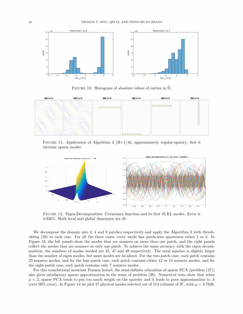
24 THOMAS Y. HOU, QIN LI, AND PENGCHUAN ZHANG
log10
|Ω(i,j)|
-12 -10 -8 -6 -4 -2 0 2
coun
ts
×104
0
2
4
6
8
10
12 Noise Level = 1e-6
log10
|Ω(i,j)|
-10 -8 -6 -4 -2 0 2
coun
ts
×105
0
2
4
6
8
10
12 Noise Level = 1e-4
Figure 10. Histogram of absolute values of entries in Ω.
ISMD: H=1/16 ISMD: H=1/16 ISMD: H=1/16 ISMD: H=1/16 ISMD: H=1/16 ISMD: H=1/16
Figure 11. Application of Algorithm 2 (H=1/16, approximately regular-sparse): first 6intrinsic sparse modes
-1 -0.8 -0.6 -0.4 -0.2 0 0.2 0.4 0.6 0.8 1
-0.4
-0.3
-0.2
-0.1
0
0.1
0.2
0.3
0.4Eigen decomposition: K = 45, Error = 4.9358%
Figure 12. Eigen-Decomposition: Covariance function and its first 45 KL modes. Error is4.936%. Both local and global dimension are 45.
We decompose the domain into 2, 4 and 8 patches respectively and apply the Algorithm 3 with thresh-olding (50) to each case. For all the three cases, every mode has patch-wise sparseness either 1 or 2. InFigure 13, the left panels show the modes that are nonzero on more than one patch, and the right panelscollect the modes that are nonzero on only one patch. To achieve the same accuracy with the eigen decom-position, the numbers of modes needed are 45, 47 and 49 respectively. The total number is slightly largerthan the number of eigen modes, but most modes are localized. For the two-patch case, each patch contains23 nonzero modes, and for the four-patch case, each patch contains either 12 or 13 nonzero modes, and forthe eight-patch case, each patch contains only 7 nonzero modes.
For this translational invariant Poisson kernel, the semi-definite relaxation of sparse PCA (problem (27))also gives satisfactory sparse approximation in the sense of problem (26). Numerical tests show that whenµ < 2, sparse PCA tends to put too much weight on the sparsity and it leads to poor approximation to A(over 90% error). In Figure 14 we plot 47 physical modes selected out of 513 columns of W , with µ = 2.7826.

A SPARSE DECOMPOSITION OF LOW RANK SYMMETRIC POSITIVE SEMI-DEFINITE MATRICES 25
-1 0 1
-1
1Sparse modes occupying more than 1 patches
-1 0 1
-0.5730
0.5730Sparse modes occupying only 1 patch
-1 -0.5 0 0.5 1
-1
1Sparse modes occupying more than 1 patches
-1 -0.5 0 0.5 1
-0.7899
0.7899Sparse modes occupying only 1 patch
-1 -0.75 -0.5 -0.25 0 0.25 0.5 0.75 1
-1
1Sparse modes occupying more than 1 patches
-1 -0.75 -0.5 -0.25 0 0.25 0.5 0.75 1
-0.9442
0.9442Sparse modes occupying only 1 patch
Figure 13. Upper: Two patches case. Error is 4.95%. Global dimension is 45 and thelocal dimension is 23 for both patches. Middle: Four patches case. Error is 4.76%. Globaldimension is 47 and the local dimension is 12, 13, 13, 12 respectively. Bottom: Eight patchescase. Error is 4.42%. Global dimension is 49 and the local dimension is 7 for all patches.
−1 −0.8 −0.6 −0.4 −0.2 0 0.2 0.4 0.6 0.8 1−0.02
0
0.02
0.04
0.06
0.08
0.1
0.1247 sparse modes from sparse density matrix W
−1 −0.8 −0.6 −0.4 −0.2 0 0.2 0.4 0.6 0.8 1−0.02
0
0.02
0.04
0.06
0.08
0.1
0.125 of the sparse modes
Figure 14. Sparse PCA: µ = 2.7826. We specifically choose 47 columns out of W andshow all and 5 of them.
The error is 4.94%. We also show 5 out of them on the right panel. Note that we have used the translationinvariance property in selecting the columns of W .
6. Conclusions and future work
In this paper, we introduced a new matrix factorization method, the intrinsic sparse mode decomposition(ISMD), to obtain a sparse decomposition of low rank symmetric positive semidefinite matrices. Insteadof minimizing the total number of nonzero entries of the decomposed modes, the ISMD minimizes thetotal patch-wise sparseness with a prescribed partition of index set [N ]. The decomposed modes from the

26 THOMAS Y. HOU, QIN LI, AND PENGCHUAN ZHANG
ISMD are called intrinsic sparse modes for the decomposed matrix with respect to the partition. TheISMD is equivalent to the eigen decomposition for the coarsest partition and recovers the pivoted Choleskydecomposition for the finest partition. If the partition is regular-sparse with respect to the matrix to bedecomposed, we prove that the ISMD gives the optimal patch-wise sparse decomposition. We also provethat as long as the partition is regular-sparse, the decomposed modes gets sparser (in the sense of l0 norm)as the partition is refined. Finally, we provide a preliminary results on perturbation analysis of the ISMDbased on the assumption that the partition is regular-sparse and the intrinsic sparse modes are identifiablewith each other. Numerical examples on synthetic data demonstrate the robustness and efficiency of theISMD.
Currently, the perturbation analysis is based on an extra assumption that roughly requires that the localeigen decomposition be well conditioned, see Eqn. (47). It would be desirable to perform a perturbationanalysis without such assumption or propose a more stable version of the ISMD. In the paper, we alsodiscussed the differences between the sparse-orthogonal matrix factorization problem (4) and the generalsparse matrix factorization problem (7). We pointed out that the ISMD is not designed to solve the generalmatrix factorization problem. The ISMD is recommended as a sparse matrix factorization method only ifthe orthoganality in decomposition coefficients U is required and an exact (or nearly exact) decomposition isdesired. Finally, we have provided a heuristic algorithm (e.g. Algorithm 3) to solve problem (3) for matrixfactorization with large noise. Ultimately, the complete resolution of this matrix factorization problem inthe presence of large noise requires a better formulation and a more robust algorithm.
Appendix A. Proof of Proposition 3.1
(1) l(ψ)k , divided into patches, can be written as l
(ψ)k = [l1,k; l2,k; · · · ; lM,k]. From the definition (29), we
have ‖lm,k‖1 = 1 if ψk|Pm6= 0 and 0 otherwise. Therefore, we obtain
‖l(ψ)k ‖1 =
M∑m=1
‖lm,k‖1 = sk(ψk;P).
Moreover, on patch Pm different ψk’s correspond to different local pieces in Ψm (when they are
identical, we keep both when constructing Ψm), and thus different columns in L(ψ)m have disjoint
supports. Therefore, different columns in L(ψ) have disjoint supports.
(2) From the definition (29), the j-th row of L(ψ)n is equal to eTkmj
, where ekmj is the kmj -th column of IK .
Then we have (L(ψ)n )TL
(ψ)n =
∑dnj=1 eknj e
Tknj
. Therefore, we obtain
(56) B(ψ)n;m ≡ L(ψ)
m (L(ψ)n )TL(ψ)
n (L(ψ)m )T =
dn∑j=1
L(ψ)m eknj (L(ψ)
m eknj )T =
dn∑j=1
lm,knj lTm,knj
,
where lm,knj is the knj -th column of L(ψ)m .
From the definition (29), lm,kmi , the kmi -th column of L(ψ)m , is equal to ei for i ∈ [dm] and all other
columns are 0. Therefore,
(57)
K∑k=1
lm,klTm,k =
dm∑i=1
lm,kmi lTm,kmi
=
dm∑i=1
eieTi = Idm .
Eqn. (56) sums over k ∈ knj dnj=1 ⊂ [K] and then we conclude that B
(ψ)n;m is diagonal with diagonal
entries either 1 or 0. Moreover, if B(ψ)n;m(i, i) = 1 the term eie
Ti has to be included in the summation
in (56). Among all terms lm,klTm,kKk=1, only lm,kmi lTm,kmi
is equal to eieTi due to the definition of
L(ψ)m . Therefore, the term lm,kmi l
Tm,kmi
has to be included in the summation in (56). Therefore, there
exists j ∈ [dn] such that knj = kmi . In other words, there exist k ∈ [K] and j ∈ [dn] such thatψk|Pm
= ψm,i and ψk|Pn= ψn,j .
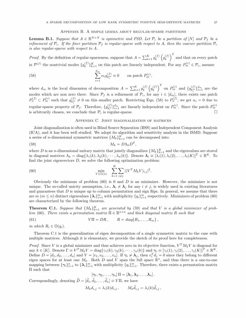
A SPARSE DECOMPOSITION OF LOW RANK SYMMETRIC POSITIVE SEMI-DEFINITE MATRICES 27
Appendix B. A simple lemma about regular-sparse partitions
Lemma B.1. Suppose that A ∈ RN×N is symmetric and PSD. Let Pc be a partition of [N ] and Pf be arefinement of Pc. If the finer partition Pf is regular-sparse with respect to A, then the coarser partition Pcis also regular-sparse with respect to A.
Proof. By the definition of regular-sparseness, suppose that A =∑Kk=1 g
(f)k
(g(f)k
)Tand that on every patch
in P(f) the nontrivial modes g(f)k Kk=1 on this patch are linearly independent. For any P(c)m ∈ Pc, assume
(58)
dm∑i=1
αig(f)kmi≡ 0 on patch P (c)
m ,
where dm is the local dimension of decomposition A =∑Kk=1 g
(f)k
(g(f)k
)Ton P
(c)m and g(f)kmi
dmi=1 are the
modes which are non zero there. Since Pf is a refinement of Pc, for any i ∈ [dm], there exists one patch
P(f)n ⊂ P
(c)m such that g
(f)kmi6= 0 on this smaller patch. Restricting Eqn. (58) to P
(f)n , we get αi = 0 due to
regular-sparse property of Pf . Therefore, g(f)kmidmi=1 are linearly independent on P
(c)m . Since the patch P
(c)m
is arbitrarily chosen, we conclude that Pc is regular-sparse.
Appendix C. Joint diagonalization of matrices
Joint diagonalization is often used in Blind Source Separation (BSS) and Independent Component Analysis(ICA), and it has been well studied. We adopt its algorithm and sensitivity analysis in the ISMD. Supposea series of n-dimensional symmetric matrices MkKk=1 can be decomposed into:
(59) Mk = DΛkDT ,
where D is an n-dimensional unitary matrix that jointly diagonalizes MkKk=1 and the eigenvalues are storedin diagonal matrices Λk = diagλ1(k), λ2(k), · · · , λn(k). Denote λi ≡ [λi(1), λi(2), . . . , λi(K)]T ∈ RK . Tofind the joint eigenvectors D, we solve the following optimization problem:
(60) minV ∈O(n)
K∑k=1
∑i 6=j
|(V TMkV )i,j |2.
Obviously the minimum of problem (60) is 0 and D is an minimizer. However, the minimizer is notunique. The so-called unicity assumption, i.e., λi 6= λj for any i 6= j, is widely used in existing literaturesand guarantees that D is unique up to column permutation and sign flips. In general, we assume that thereare m (m ≤ n) distinct eigenvalues λimi=1 with multiplicity qimi=1 respectively. Minimizers of problem (60)are characterized by the following theorem.
Theorem C.1. Suppose that MkKk=1 are generated by (59) and that V is a global minimizer of prob-lem (60). There exists a permutation matrix Π ∈ Rn×n and block diagonal matrix R such that
(61) VΠ = DR , R = diagR1, . . . , Rm ,in which Ri ∈ O(qi).
Theorem C.1 is the generalization of eigen decomposition of a single symmetric matrix to the case withmultiple matrices. Although it is elementary, we provide the sketch of its proof here for completeness.
Proof. Since V is a global minimizer and thus achieves zero in its objective function, V TMkV is diagonal forany k ∈ [K]. Denote Γ ≡ V TMkV = diagγ1(k), γ2(k), · · · , γn(k) and γi ≡ [γi(1), γi(2), . . . , γi(K)]T ∈ RK .Define D = [d1, d2, . . . , dn] and V = [v1, v2, . . . , vn]. If γi 6= λj , then vTi dj = 0 since they belong to differenteigen spaces for at least one Mk. Both D and V span the full space Rn, and thus there is a one-to-onemapping between γini=1 to λimi=1 with multiplicity qimi=1. Therefore, there exists a permutation matrixΠ such that
[γ1,γ2, . . . ,γn] Π = [λ1,λ2, . . . ,λn] .
Correspondingly, denoting D = [d1, d2, . . . , dn] ≡ VΠ, we have
Mkdi,j = λi(k)di,j , Mkdi,j = λi(k)di,j ,

28 THOMAS Y. HOU, QIN LI, AND PENGCHUAN ZHANG
where di,jqij=1 and di,jqij=1 are the eigenvectors in D and D respectively corresponding to the eigenvalue
λi. By orthogonality between eigenspaces and completeness of D and D, di,jqij=1 and di,jqij=1 must
span the same qi-dimensional subspace. Since both di,jqij=1 and di,jqij=1 are orthonormal, there exists
Ri ∈ O(qi) such that di,j = Ridi,j for j ∈ [qi].
The sensitivity analysis of the joint diagonalization problem (60) is studied in [5], and we directly quoteits main results below.
Proposition C.1. Suppose that MkKk=1 are generated as follows:
Mk = Mk + εMk, Mk = DΛkDT ,
where D is unitary, ε is a real scalar, matrices Mk are arbitrary and matrices Λk are diagonal as in (59).Suppose that the unicity assumption, i.e., λi 6= λj for any i 6= j, holds true. Then any solution of the joint
diagonalization problem (60) with the perturbed input MkKk=1, denoted by D, is in the form
D = D(I + εE + o(ε))J
where J is the product of a permutation matrix with a diagonal matrix having only ±1 on its diagonal. MatrixE has a null diagonal and is antisymmetric, i.e., E + ET = 0. Its off-diagonal entries Eij are give by
Eij =1
2
K∑k=1
fij(k)dTi (Mk + MTk )dj , with fij(k) =
λj(k)− λi(k)∑Kl=1(λj(l)− λi(l))2
.
In this paper, we solve problem (60) using a Jacobi-like algorithm proposed in [4, 2]. The idea is toperform 2-dimensional rotation to reduce the amplitude of the off-diagonal pairs one by one. Denote byR = R(p, q, c, s) the 2-dimensional rotation that deals with (p, q) entries of Mk:
(62) R = R(p, q, c, s) = I + (c− 1)epeTp − seqeTq + seqe
Tp + (c− 1)epe
Tq ,
where c2 + s2 = 1 for unitarity. A simple calculation shows that
K∑k=1
∑i 6=j
|(RTMkR)i,j |2 =
K∑k=1
∑i 6=j
|Mk(i, j)|2 −K∑k=1
(|Mk(p, q)|2 + |Mk(q, p)|2
)+
K∑k=1
(sc(Mk(q, q)−Mk(p, p)) + c2Mk(p, q)− s2Mk(q, p)
)2+
K∑k=1
(sc(Mk(q, q)−Mk(p, p))− s2Mk(p, q) + c2Mk(q, p)
)2.
(63)
It can be shown that the choice of c and s that minimizes (63) also minimizes ‖Lpqz‖2 where z =[c2 − s2, 2cs
]Tis a 2× 1 vector, and
(64) Lpq :=
M1(p, q) M1(q,q)−M1(p,p)2
......
MK(p, q) MK(q,q)−MK(p,p)2
,is a K × 2 matrix. It is apparent that the singular vector corresponding to the smallest singular value doesthe job. Denote this singular vector by w with w(1) ≥ 0. The optimizer of Eqn. (63) is given by:
(65) c =
√1 +w(1)
2, s =
w(2)
2c.
We perform such rotation for each pair of (p, q) until the algorithm converges, as shown in Algorithm 4.The algorithm has been shown to have quadratic asymptotic convergence rate and is numerically stable,see [2].

A SPARSE DECOMPOSITION OF LOW RANK SYMMETRIC POSITIVE SEMI-DEFINITE MATRICES 29
Algorithm 4 Jacobi-like Joint Diagonalization
Require: ε > 0; MkKk=1, which are symmetric and jointly diagonalizable.
Ensure: V ∈ O(n) such that∑Kk=1
∑i 6=j |(V TMkV )i,j |2 ≤ ε
∑Kk=1 ‖Mk‖2F .
1: V ← I2: while
∑Kk=1
∑i 6=j |(V TMkV )i,j |2 > ε
∑Kk=1 ‖Mk‖2F do
3: for p = 1, 2, · · · , n do4: for q = p+ 1, p+ 2, · · · , n do5: define Lpq as in (64)6: compute w, the normalized singular vector corresponding to the smallest singular value
7: set c =√
1+w(1)2 , s = w(2)
2c and R = R(p, q, c, s)
8: set V ← V R; Mk ← V TMkV for k = 1, 2, · · · ,K9: end for
10: end for11: end while
Appendix D. Proof of Lemma 4.1
We point out that for the noiseless case, the ISMD in fact solves the following optimization problem toobtain Gm:
(66)
minGm∈R|Pm|×Km
M∑n=1
∑i 6=j
|Bn;m(i, j)|2
s.t. GmGTm = Amm ,
Bn;m = G†mAmnA†nnA
Tmn
(G†m)T,
in which
(67) G†m = (GTmGm)−1GTm, A†nn =
Kn∑i=1
γ−1n,ihn,ihTn,i
is the (Moore-Penrose) pseudo-inverse of Gm and Ann respectively. The ISMD solves this optimizationproblem in two steps:
(1) Perform eigen decomposition Amm = HmHTm. Then the feasible Gm can be written as HmDm with
unitary matrix Dm.(2) Find the rotation Dm which solves the joint diagonalization problem (13).
Similarly, one can check that for the noisy case, the ISMD (with truncated eigen decomposition (10)) solves
the same optimization problem with perturbed input to obtain Gm:
(68)
minGm∈R|Pm|×Km
M∑n=1
∑i 6=j
|Bn;m(i, j)|2
s.t. GmGTm = A(t)
mm ,
Bn;m = G†mAmn
(A(t)nn
)†ATmn
(G†m)T,
where, A(t)nn is the truncated Ann defined in Eqn. (46) and
(69)(A(t)nn
)†=
Kn∑i=1
γ−1n,i hn,ihTn,i
is the pseudo-inverse of A(t)nn.
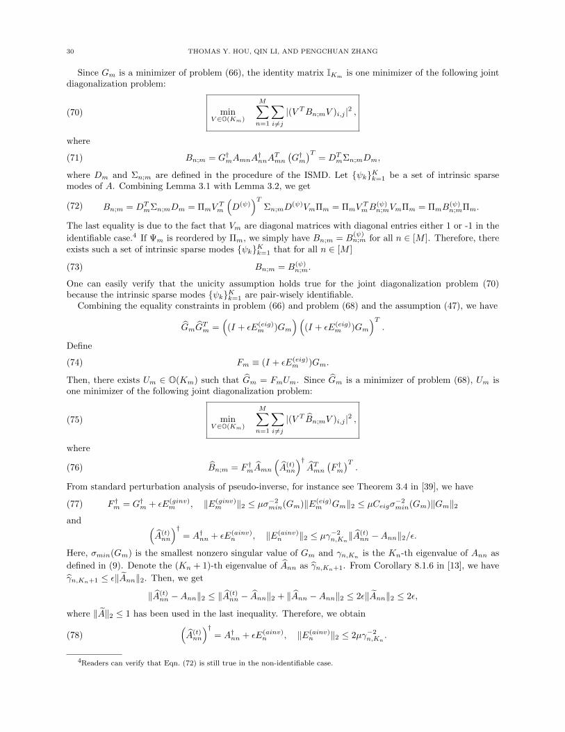
30 THOMAS Y. HOU, QIN LI, AND PENGCHUAN ZHANG
Since Gm is a minimizer of problem (66), the identity matrix IKm is one minimizer of the following jointdiagonalization problem:
(70) minV ∈O(Km)
M∑n=1
∑i 6=j
|(V TBn;mV )i,j |2 ,
where
(71) Bn;m = G†mAmnA†nnA
Tmn
(G†m)T
= DTmΣn;mDm,
where Dm and Σn;m are defined in the procedure of the ISMD. Let ψkKk=1 be a set of intrinsic sparsemodes of A. Combining Lemma 3.1 with Lemma 3.2, we get
Bn;m = DTmΣn;mDm = ΠmV
Tm
(D(ψ)
)TΣn;mD
(ψ)VmΠm = ΠmVTmB
(ψ)n;mVmΠm = ΠmB
(ψ)n;mΠm.(72)
The last equality is due to the fact that Vm are diagonal matrices with diagonal entries either 1 or -1 in the
identifiable case.4 If Ψm is reordered by Πm, we simply have Bn;m = B(ψ)n;m for all n ∈ [M ]. Therefore, there
exists such a set of intrinsic sparse modes ψkKk=1 that for all n ∈ [M ]
(73) Bn;m = B(ψ)n;m.
One can easily verify that the unicity assumption holds true for the joint diagonalization problem (70)because the intrinsic sparse modes ψkKk=1 are pair-wisely identifiable.
Combining the equality constraints in problem (66) and problem (68) and the assumption (47), we have
GmGTm =
((I + εE(eig)
m )Gm
)((I + εE(eig)
m )Gm
)T.
Define
(74) Fm ≡ (I + εE(eig)m )Gm.
Then, there exists Um ∈ O(Km) such that Gm = FmUm. Since Gm is a minimizer of problem (68), Um isone minimizer of the following joint diagonalization problem:
(75) minV ∈O(Km)
M∑n=1
∑i 6=j
|(V T Bn;mV )i,j |2 ,
where
(76) Bn;m = F †mAmn
(A(t)nn
)†ATmn
(F †m)T.
From standard perturbation analysis of pseudo-inverse, for instance see Theorem 3.4 in [39], we have
(77) F †m = G†m + εE(ginv)m , ‖E(ginv)
m ‖2 ≤ µσ−2min(Gm)‖E(eig)m Gm‖2 ≤ µCeigσ−2min(Gm)‖Gm‖2
and (A(t)nn
)†= A†nn + εE(ainv)
n , ‖E(ainv)n ‖2 ≤ µγ−2n,Kn
‖A(t)nn −Ann‖2/ε.
Here, σmin(Gm) is the smallest nonzero singular value of Gm and γn,Knis the Kn-th eigenvalue of Ann as
defined in (9). Denote the (Kn + 1)-th eigenvalue of Ann as γn,Kn+1. From Corollary 8.1.6 in [13], we have
γn,Kn+1 ≤ ε‖Ann‖2. Then, we get
‖A(t)nn −Ann‖2 ≤ ‖A(t)
nn − Ann‖2 + ‖Ann −Ann‖2 ≤ 2ε‖Ann‖2 ≤ 2ε,
where ‖A‖2 ≤ 1 has been used in the last inequality. Therefore, we obtain
(78)(A(t)nn
)†= A†nn + εE(ainv)
n , ‖E(ainv)n ‖2 ≤ 2µγ−2n,Kn
.
4Readers can verify that Eqn. (72) is still true in the non-identifiable case.

A SPARSE DECOMPOSITION OF LOW RANK SYMMETRIC POSITIVE SEMI-DEFINITE MATRICES 31
When ε 1, the constant µ can be taken as 2 in both (77) and (78). Combining (45), (77) and (78), we get
Bn;m =Bn;m + εBn;m ,
Bn;m =E(ginv)m AmnA
†nnA
Tmn
(G†m)T
+G†mAmnA†nnA
Tmn
(G†m)T
+G†mAmnE(ainv)n ATmn
(G†m)T
+G†mAmnA†nnA
Tmn
(G†m)T
+G†mAmnA†nnA
Tmn
(E(ginv)m
)T.
(79)
By Proposition C.1, there exists E(jd)m ∈ RKm×Km such that
Um = (IKm + εE(jd)m + o(ε))Jm,
where Jm is the product of a permutation matrix with a diagonal matrix having only ±1 on its diagonal.
Matrix E(jd)m has a null diagonal and is antisymmetric, i.e., E
(jd)m +
(E
(jd)m
)T= 0. Its off-diagonal entries
E(jd)m (i, j) are given by
E(jd)m (i, j) =
M∑n=1
f(n) Bn;m , with fij(n) =Bn;m(j, j)−Bn;m(i, i)∑M
n=1(Bn;m(j, j)−Bn;m(i, i))2.
Here, f(n) is the matrix with entries fij(n) and f(n) Bn;m is the matrix point-wise product (also known
as the Hadamard product). Notice that we take advantage of the fact that Bn;m is symmetric to simplify
E(jd)m (i, j). Since Bn;m(j, j) − Bn;m(i, i) is either ±1 or 0, |fij(n)| ≤ 1 for any i,j and n, and thus we have‖f(n)‖F ≤ Km. Therefore, we conclude
(80) ‖E(jd)m ‖F ≤
M∑n=1
‖f(n) Bn;m‖F ≤M∑n=1
‖f(n)‖F ‖Bn;m‖F ≤ K3/2m
M∑n=1
‖Bn;m‖2,
where we have used triangle inequality, ‖f(n) Bn;m‖F ≤ ‖f(n)‖F ‖Bn;m‖F and ‖Bn;m‖F ≤ K1/2m ‖Bn;m‖2
in deriving the above inequalities. Combining (79), (45), (77) and (78), we know that ‖Bn;m‖2 are boundedby a constant, denoted by Cjd, which only depends on A and Ceig. From the assumption (47), Ceig is a
constant depending on A but not on ε or A. Therefore, Cjd depends only on A but not on ε or A.
Acknowledgments
This research was in part supported by Air Force MURI Grant FA9550-09-1-0613, DOE grant DE-FG02-06ER257, and NSF Grants No. DMS-1318377, DMS-1159138.
References
[1] Deepak Agarwal and Bee-Chung Chen. Regression-based latent factor models. In Proceedings of the 15th ACM SIGKDDinternational conference on Knowledge discovery and data mining, pages 19–28. ACM, 2009.
[2] Angelika Bunse-Gerstner, Ralph Byers, and Volker Mehrmann. Numerical methods for simultaneous diagonalization. SIAMJournal on Matrix Analysis and Applications, 14(4):927–949, 1993.
[3] Emmanuel J. Candes, Xiaodong Li, Yi Ma, and John Wright. Robust principal component analysis? Journal of the ACM,
58(3):11:1–11:37, June 2011.[4] J. F. Cardoso and A. Souloumiac. Blind beamforming for non-gaussian signals. IEE Proceedings F (Radar and Signal
Processing), 140(6):362–370(8), December 1993.[5] Jean-Francois Cardoso. Perturbation of joint diagonalizers. Technical Report 94D023, Signal Department, Telecom Paris,
Paris, 1994.
[6] Venkat Chandrasekaran, Sujay Sanghavi, Pablo A. Parrilo, and Alan S. Willsky. Rank-sparsity incoherence for matrix
decomposition. SIAM Journal on Optimization, 21(2):572–596, April 2011.[7] Yi Chen, John Jakeman, Claude Gittelson, and Dongbin Xiu. Local polynomial chaos expansion for linear differential
equations with high dimensional random inputs. SIAM Journal on Scientific Computing, 37(1):A79–A102, 2015.[8] A. d’Aspremont, L. El Ghaoui, M. Jordan, and G. Lanckriet. A direct formulation for sparse pca using semidefinite
programming. SIAM Review, 49(3):434–448, 2007.
[9] Yalchin Efendiev, Juan Galvis, and Xiao-Hui Wu. Multiscale finite element methods for high-contrast problems using localspectral basis functions. Journal of Computational Physics, 230(4):937–955, 2011.
[10] Juan Galvis and Yalchin Efendiev. Domain decomposition preconditioners for multiscale flows in high contrast media:
Reduced dimension coarse spaces. Multiscale Modeling & Simulation, 8(5):1621–1644, January 2010.[11] Chuan Gao and Barbara E Engelhardt. A sparse factor analysis model for high dimensional latent spaces. In NIPS:
Workshop on Analysis Operator Learning vs. Dictionary Learning: Fraternal Twins in Sparse Modeling, 2012.

32 THOMAS Y. HOU, QIN LI, AND PENGCHUAN ZHANG
[12] Mehdi Ghommem, Michael Presho, Victor M. Calo, and Yalchin Efendiev. Mode decomposition methods for flows inhigh-contrast porous media. global–local approach. Journal of Computational Physics, 253:226–238, November 2013.
[13] G.H. Golub and C.F. Van Loan. Matrix Computations. Matrix Computations. Johns Hopkins University Press, 2012.
[14] Thomas Y. Hou and Xiao-Hui Wu. A multiscale finite element method for elliptic problems in composite materials andporous media. Journal of Computational Physics, 134(1):169 – 189, 1997.
[15] Thomas Y. Hou, Xiao-Hui Wu, and Yu Zhang. Removing the cell resonance error in the multiscale finite element methodvia a petrov-galerkin formulation. Communications in Mathematical Sciences, 2(2):185–205, 06 2004.
[16] Y. Thomas Hou, Qin Li, and Pengchuan Zhang. Exploring the locally low dimensional structure in solving random elliptic
pdes. Multiscale Modeling & Simulation, 2016.[17] Y. Thomas Hou and Pengchuan Zhang. Sparse operator compression of elliptic operators – part i : Second order elliptic
operators. preprint, 2016.
[18] Y. Thomas Hou and Pengchuan Zhang. Sparse operator compression of elliptic operators – part ii : High order ellipticoperators. preprint, 2016.
[19] Rodolphe Jenatton, Guillaume Obozinski, and Francis R Bach. Structured sparse principal component analysis. In
AISTATS, pages 366–373, 2010.[20] Ian T. Jolliffe, Nickolay T. Trendafilov, and Mudassir Uddin. A modified principal component technique based on the lasso.
Journal of Computational and Graphical Statistics, 12(3):pp. 531–547, 2003.
[21] IT Jolliffe, M Uddin, and SK Vines. Simplified eofs three alternatives to rotation. Climate Research, 20(3):271–279, 2002.
[22] K. Karhunen. Uber lineare Methoden in der Wahrscheinlichkeitsrechnung. Annales Academiae scientiarum Fennicae: Math-
ematica - Physica. Universitat Helsinki, 1947.
[23] W Kohn. Image of the fermi surface in the vibration spectrum of a metal. Physical Review Letters, 2(9):393, 1959.[24] W.J. Krzanowski and F.H.C. Marriott. Multivariate Analysis: Kendall’s Library of Statistics, Volume 2. Kendall’s advanced
theory of statistics. Wiley, 1995.[25] R. Lai, J. Lu, and S. Osher. Density matrix minimization with L1 regularization. Communications in Mathematical
Sciences, to appear.
[26] Daniel D Lee and H Sebastian Seung. Learning the parts of objects by non-negative matrix factorization. Nature,401(6755):788–791, 1999.
[27] Honglak Lee, Alexis Battle, Rajat Raina, and Andrew Y Ng. Efficient sparse coding algorithms. In Advances in neuralinformation processing systems, pages 801–808, 2006.
[28] Richard B Lehoucq and Danny C Sorensen. Deflation techniques for an implicitly restarted arnoldi iteration. SIAM Journal
on Matrix Analysis and Applications, 17(4):789–821, 1996.
[29] Michel Loeve. Probability Theory I. Comprehensive Manuals of Surgical Specialties. Springer, 1977.[30] Craig Lucas. Lapack-style codes for level 2 and 3 pivoted cholesky factorizations. LAPACK Working, 2004.
[31] Xi Luo. High dimensional low rank and sparse covariance matrix estimation via convex minimization. arXiv preprintarXiv:1111.1133, 2011.
[32] Julien Mairal, Francis Bach, Jean Ponce, and Guillermo Sapiro. Online learning for matrix factorization and sparse coding.
Journal of Machine Learning Research, 11(Jan):19–60, 2010.[33] Nicola Marzari, Arash A Mostofi, Jonathan R Yates, Ivo Souza, and David Vanderbilt. Maximally localized wannier
functions: Theory and applications. Reviews of Modern Physics, 84(4):1419, 2012.
[34] Nicola Marzari and David Vanderbilt. Maximally localized generalized wannier functions for composite energy bands.Physical review B, 56(20):12847, 1997.
[35] Houman Owhadi. Multi-grid with rough coefficients and multiresolution operator decomposition from hierarchical infor-
mation games. arXiv preprint arXiv:1503.03467, 2015.[36] Houman Owhadi, Lei Zhang, and Leonid Berlyand. Polyharmonic homogenization, rough polyharmonic splines and sparse
super-localization. ESAIM: Mathematical Modelling and Numerical Analysis, 48(02):517–552, 2014.
[37] Vidvuds Ozolins, Rongjie Lai, Russel Caflisch, and Stanley Osher. Compressed modes for variational problems in mathe-matics and physics. Proceedings of the National Academy of Sciences, 110(46):18368–18373, 2013.
[38] Danny C Sorensen. Implicit application of polynomial filters in ak-step arnoldi method. Siam journal on matrix analysisand applications, 13(1):357–385, 1992.
[39] GW Stewart. On the perturbation of pseudo-inverses, projections and linear least squares problems. SIAM review,19(4):634–662, 1977.
[40] Vincent Q Vu, Juhee Cho, Jing Lei, and Karl Rohe. Fantope projection and selection: A near-optimal convex relaxation
of sparse pca. In Advances in Neural Information Processing Systems, pages 2670–2678, 2013.
[41] Andrew Wagner, John Wright, Arvind Ganesh, Zihan Zhou, Hossein Mobahi, and Yi Ma. Toward a practical face recognitionsystem: Robust alignment and illumination by sparse representation. Pattern Analysis and Machine Intelligence, IEEE
Transactions on, 34(2):372–386, 2012.[42] Gregory H Wannier. The structure of electronic excitation levels in insulating crystals. Physical Review, 52(3):191, 1937.[43] E Weinan, Tiejun Li, and Jianfeng Lu. Localized bases of eigensubspaces and operator compression. Proceedings of the
National Academy of Sciences, 107(4):1273–1278, 2010.
[44] Daniela M Witten, Robert Tibshirani, and Trevor Hastie. A penalized matrix decomposition, with applications to sparseprincipal components and canonical correlation analysis. Biostatistics, page kxp008, 2009.
[45] Youwei Zhang, Alexandre d’Aspremont, and Laurent El Ghaoui. Sparse pca: Convex relaxations, algorithms and applica-tions. In Handbook on Semidefinite, Conic and Polynomial Optimization, pages 915–940. Springer, 2012.

A SPARSE DECOMPOSITION OF LOW RANK SYMMETRIC POSITIVE SEMI-DEFINITE MATRICES 33
[46] Hui Zou, Trevor Hastie, and Robert Tibshirani. Sparse principal component analysis. Journal of Computational andGraphical Statistics, 15:265–286, 2004.