A SOM based Anomaly Detection Method for Wind … Journal of Prognostics and Health Management, ISSN...

International Journal of Prognostics and Health Management, ISSN 2153-2648, 2016 029

A SOM based Anomaly Detection Method for Wind Turbines

Health Management through SCADA Data

Mian Du1,2,3, Lina Bertling Tjernberg3, Shicong Ma1, Qing He1, Lin Cheng2 and Jianbo Guo1

1China Electric Power Research Institute, Beijing, Haidian, 100192, China

[email protected]

2Department of Electrical Engineering, Tsinghua University, Beijing, Haidian, 100084, China

3KTH Royal Institute of Technology, Stockholm, Sweden

ABSTRACT

In this paper, a data driven method for Wind Turbine system

level anomaly detection and root sub-component

identification is proposed. Supervisory control and data

acquisition system (SCADA) data of WT is adopted and

several parameters are selected based on physical

knowledge in this domain and correlation coefficient

analysis to build a normal behavior model. This model

which is based on Self-organizing map (SOM) projects

higher-dimensional SCADA data into a two-dimension-map.

Afterwards, the Euclidean distance based indicator for

system level anomalies is defined and a filter is created to

screen out suspicious data points based on quantile function.

Moreover, a failure data pattern based criterion is created

for anomaly detection from system level. In order to track

which sub-component should be responsible for an anomaly,

a contribution proportion (CP) index is proposed. The

method is tested with a two-month SCADA dataset with the

measurement interval as 20 seconds. Results demonstrate

capability and efficiency of the proposed method.

1. INTRODUCTION

Wind energy is considered an effective way to relieve the

carbon dioxide risk caused by consuming traditional fossil

resources. According to the statistics on wind energy

published by the European wind energy association in Feb.

2016 (European Wind Energy Association, 2016), until

2015, 142GW of wind energy in total has been installed in

Europe and 11GW of it includes offshore. Moreover, what

should be considered as milestone is that in 2015, wind

energy has substituted hydro as the third largest power

source in the European Union (EU) with 15.6% share of

total power capacity. Figure 1 shows the annual installation

of both onshore and offshore wind energy in EU.

Wind turbines are capital-intensive equipment compared to

conventional fossil resource based technologies such as

natural gas power generators, where as much as 25-30% of

costs are related to operations and maintenance (O&M)

(Milborrow, 2006). Due to the huge amount of O&M cost of

a wind farm, keeping WTs working efficiently and

formulating cost effective maintenance schedules are the

main interests of shareholders, especially in offshore wind

farms.

While realizing the objective of decreasing the O&M cost

needs various information, one of the most significant part

is the health condition of wind turbines. In recently

published papers (de Azevedo, Araújo, & Bouchonneau,

2016) and (Kandukuri, Karimi, & Robbersmyr, 2016),

related excellent works have been introduced. Based on

adopted approaches, research on wind turbine health

condition monitoring can generally be classified as two

Figure 1. Annual onshore and offshore wind energy

installation (MW) (European Wind Energy Association,

2016)

_____________________

Mian Du et al. This is an open-access article distributed under the terms of the Creative Commons Attribution 3.0 United States License, which

permits unrestricted use, distribution, and reproduction in any medium,

provided the original author and source are credited.

INTERNATIONAL JOURNAL OF PROGNOSTICS AND HEALTH MANAGEMENT

2

main branches, data driven approach (Sun, Li, Wang, & Lei,

2016) and analytical approach (Bruce, Long, & Dwyer-

Joyce, 2015).

While a physic based analytical model is easier for

understanding and interpretation, the nonlinear relationship

among the subcomponents of a wind turbine make it

difficult to model a wind turbine from a system level (de

Bessa, Palhares, D'Angelo, & Chaves Filho). Even though

in (Breteler, Kaidis, Tinga, & Loendersloot, 2015) a system

level physics based model is proposed for failure prognosis,

it still keeps the assumption that each component works

independently. Moreover, the component failure detection

in that paper is still based on data from condition monitoring

system (CMS) and supervisory control and data acquisition

system (SCADA). As access to wind turbine O&M data is

much easier with the development of advanced sensor

technology, system level methods for wind turbine health

management are more preferable from O&M perspective.

Data driven approach from a system level perception is

attracting more interest in research field (de Bessa, Palhares,

D'Angelo, & Chaves Filho) (Sun, Li, Wang, & Lei, 2016)

(de Andrade Vieira & Sanz-Bobi, 2013) (Marhadi &

Skrimpas, 2015).

Considering the data type adopted in this field, vibration

data (Yang, et al., 2016), acoustic data (Park, Sohn,

Malinowski, & Ostachowicz, 2016) and SCADA data

(Schlechtingen, Santos, & Achiche, 2013) are most widely

used in recent published papers. Comparing with the

previous two data resources, SCADA data has

comprehensive information of nearly all subcomponents and

is pointed out to be the most economic data resource for

developing a CMS for wind turbines (Xiang, Watson, & Liu,

2009). Besides, there is a large amount of SCADA data

available which contains both wind turbine operation status

and measurements of signals as temperature, pressure,

voltage and current. From a practical point of view, a

SCADA system is constituted by many sensors distributed

to each subcomponent. For some key components as

generator, gear box and rotor system, several sensors are

equipped to get more thorough information (Sun, Li, Wang,

& Lei, 2016). Therefore, monitoring operation status and

health condition through SCADA data is more cost-effective.

Considering various data-driven methods, such as neural

network (NN) (de Andrade Vieira & Sanz-Bobi, 2013),

fuzzy based approach (Sun, Li, Wang, & Lei, 2016), support

vector machine (SVM) (Santos, Villa, Reñones, Bustillo, &

Maudes, 2015), and Bayesian network based approach

(Schlechtingen, Santos, & Achiche, 2013) have been used to

model wind turbine behavior with SCADA data. Although

each approach has advantages and limitations, great findings

have been provided by the previous papers. In (Santos, Villa,

Reñones, Bustillo, & Maudes, 2015), a SVM based solution

is created for failure detection with classification of

operational states of a wind turbine. While in (Castellani,

Astolfi, Sdringola, Proietti, & Terzi, 2015), the directional

behavior of a wind turbine is analyzed through SCADA data

to build connection between the alignments of wind turbines

and performance deviations.

Since SOM based failure detection and prognostic and

health management have been widely researched, previous

works should be addressed here. In (Lamedica, Prudenzi,

Sforna, Caciotta, & Cencellli, 1996), a short term

anomalous load periods prediction technique is proposed.

SOM is used for historical loads data classification. In

(Hoglund, Hatonen, & Sorvari, 2000), a computer-host

based anomaly detection system is developed while SOM is

used to learn the normal behavior from a set of features

describing the object. With similar idea, authors in (Fabio A

& Dipankar, 2003) and (Depren, Topallar, Anarim, & Ciliz,

2005) develop failure and intrusion detection system for

different applications. Moreover, in (Tian, Azarian, & Pecht,

2014), k-nearest neighbor (KNN) algorithm is used to

improve SOM for failure detection. SOM can also be used

for developing monitoring systems. In (Rigamonti, Zio,

Alessi, Astigarraga, & Galarza, 2015), a monitoring system

for operating insulated bipolar transistors is proposed based

on SOM. While in (Zhong, Wang, Wu, Zhou, & Jin, 2016),

a SOM based monitoring system is developed solve the

visualization monitoring and fault diagnosis problem in

chemical industry process. Hence, the general idea that

using SOM to capture the features of the normal behavior of

an object is powerful in anomaly detection. And this idea is

also suit to data driven approach based wind turbine

anomaly detection, as failure data is usually not sufficient

enough for researchers to catch the failure patterns.

Considering SOM based wind turbine anomaly detection,

many works have been published. In (Zhao, Siegel, Lee, &

Su, 2013), condition monitoring system (CMS) data and

SCADA data are used for developing a component level

degradation assessment and fault localization framework.

However, as is mentioned above CMS is not always

available for some wind turbines and it also means more

investment for installing devices to get the data. In

(Wilkinson, Darnell, Delft, & Harman, 2014), a comparison

study is conducted among NN, SOM and physical model

based wind turbine condition monitoring with SCADA data.

However, it fails to define the abnormal conditions after the

deviation is calculated. Moreover, in (Chen, 2014), the

author provides a comprehensive study on wind turbine

monitoring using SCADA data. However, SOM is only used

as classification tool to distinguish operation states. Experts

are required to interpret the results.

Inspired by the previous works, we try to make small steps

forward in this field. The main difference of this work is

that it proposed a top-down method which is capable of

detecting system level anomaly and locating the rooted

subcomponent. In this work, self-organizing map (SOM) is

adopted to model the normal behavior of a wind turbine by


3

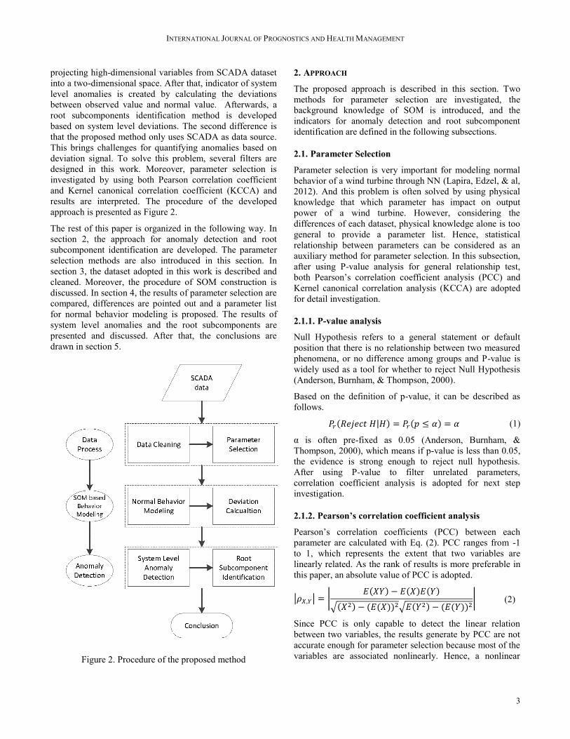
projecting high-dimensional variables from SCADA dataset

into a two-dimensional space. After that, indicator of system

level anomalies is created by calculating the deviations

between observed value and normal value. Afterwards, a

root subcomponents identification method is developed

based on system level deviations. The second difference is

that the proposed method only uses SCADA as data source.

This brings challenges for quantifying anomalies based on

deviation signal. To solve this problem, several filters are

designed in this work. Moreover, parameter selection is

investigated by using both Pearson correlation coefficient

and Kernel canonical correlation coefficient (KCCA) and

results are interpreted. The procedure of the developed

approach is presented as Figure 2.

The rest of this paper is organized in the following way. In

section 2, the approach for anomaly detection and root

subcomponent identification are developed. The parameter

selection methods are also introduced in this section. In

section 3, the dataset adopted in this work is described and

cleaned. Moreover, the procedure of SOM construction is

discussed. In section 4, the results of parameter selection are

compared, differences are pointed out and a parameter list

for normal behavior modeling is proposed. The results of

system level anomalies and the root subcomponents are

presented and discussed. After that, the conclusions are

drawn in section 5.

Figure 2. Procedure of the proposed method

2. APPROACH

The proposed approach is described in this section. Two

methods for parameter selection are investigated, the

background knowledge of SOM is introduced, and the

indicators for anomaly detection and root subcomponent

identification are defined in the following subsections.

2.1. Parameter Selection

Parameter selection is very important for modeling normal

behavior of a wind turbine through NN (Lapira, Edzel, & al,

2012). And this problem is often solved by using physical

knowledge that which parameter has impact on output

power of a wind turbine. However, considering the

differences of each dataset, physical knowledge alone is too

general to provide a parameter list. Hence, statistical

relationship between parameters can be considered as an

auxiliary method for parameter selection. In this subsection,

after using P-value analysis for general relationship test,

both Pearson’s correlation coefficient analysis (PCC) and

Kernel canonical correlation analysis (KCCA) are adopted

for detail investigation.

2.1.1. P-value analysis

Null Hypothesis refers to a general statement or default

position that there is no relationship between two measured

phenomena, or no difference among groups and P-value is

widely used as a tool for whether to reject Null Hypothesis

(Anderson, Burnham, & Thompson, 2000).

Based on the definition of p-value, it can be described as

follows.

𝑃𝑟(𝑅𝑒𝑗𝑒𝑐𝑡 𝐻|𝐻) = 𝑃𝑟(𝑝 ≤ 𝛼) = 𝛼 (1)

α is often pre-fixed as 0.05 (Anderson, Burnham, &

Thompson, 2000), which means if p-value is less than 0.05,

the evidence is strong enough to reject null hypothesis.

After using P-value to filter unrelated parameters,

correlation coefficient analysis is adopted for next step

investigation.

2.1.2. Pearson’s correlation coefficient analysis

Pearson’s correlation coefficients (PCC) between each

parameter are calculated with Eq. (2). PCC ranges from -1

to 1, which represents the extent that two variables are

linearly related. As the rank of results is more preferable in

this paper, an absolute value of PCC is adopted.

|𝜌𝑋,𝑌| = |𝐸(𝑋𝑌) − 𝐸(𝑋)𝐸(𝑌)

√(𝑋2) − (𝐸(𝑋))2√𝐸(𝑌2) − (𝐸(𝑌))2| (2)

Since PCC is only capable to detect the linear relation

between two variables, the results generate by PCC are not

accurate enough for parameter selection because most of the

variables are associated nonlinearly. Hence, a nonlinear


4

relation method, Kernel canonical correlation analysis

(KCCA) is also included in this work to compare with PCC.

2.1.3. Kernel canonical correlation analysis

KCCA is based on Canonical correlation analysis (CCA),

but use Kernels which are functions to map the data into a

higher-dimensional feature space. In this manner, it

overcomes the drawback that CCA sometimes fails to

extract meaningful description of the data due to the

linearity of CCA method (Hardoon, Szedmak, & Shawe-

Taylor, 2004).

The Kernel function is defined as

𝐾(𝑣, 𝑧) = ⟨∅(𝑣) ∙ ∅(𝑧)⟩ (3)

in which, 𝑣 𝑎𝑛𝑑 𝑧 are variables and ∅(𝑣) 𝑎𝑛𝑑 ∅(𝑧)

represent the vectors of 𝑣 𝑎𝑛𝑑 𝑧. " ∙ " means inner product.

Consider 𝑋𝑎𝑛𝑑 𝑌 are two parameters from a SCADA

dataset, after using Kernel function to map them into a

higher-dimension, which can be represented as 𝑋′𝑎𝑛𝑑 𝑌′ , the correlation can be calculated in the following way.

𝜌 = max𝛼 𝛽

𝛼′𝑋𝑋′𝑌𝑌′𝛽

√𝛼′𝑋𝑋′𝑋𝑋′𝛼 ∙ 𝛽′𝑌𝑌′𝑌𝑌′𝛽 (4)

where 𝛼 𝑎𝑛𝑑 𝛽are the direction parameters. The estimation

algorithm of 𝜌 is introduced in (Hardoon, Szedmak, &

Shawe-Taylor, 2004).

2.2. Wind Turbine Normal Behavior Modeling with

SOM

SOM is a sub variant of neural network with unsupervised

learning properties. In this paper, the property that it can

project a dataset with high dimensional feature into one or

two dimensional space is adopted to catch the patterns of

input training data (Kohonen, 1982). Before introducing the

procedure of training SOM, definition of Best Match Unit

(BMU) must be clarified as it the key point of this paper.

Definition of BMU: a BMU is the neuron whose weight

vector has the smallest distance measure from the input

data.

Considering 𝑥 = [𝑥1, 𝑥2 … , 𝑥𝑛]𝑇 as the input vector for

training iterations, 𝑥𝑖 represents the parameters selected

from the original dataset. Moreover, 𝑤𝑖 denotes the weight

of each neuron, while 𝑤𝑖 = [𝑤𝑖1, 𝑤𝑖2 , … , 𝑤𝑖𝑛] 𝑖 = 1,2, … 𝑚.

Dimension of the weight vector equal to the number of the

input parameters.

For each training step, the distribution of neurons is updated

as follows.

‖𝑥 − 𝑤𝑢‖ = 𝑚𝑖𝑛{‖𝑥 − 𝑤𝑖‖} 𝑓𝑜𝑟 𝑎𝑙𝑙 𝑖 = 1,2, … , 𝑚 (5)

In this equation, 𝑤𝑢 represents the updated neuron weights

for next iteration. And ‖∙‖ is the distance between the input

vector and the neuron. After it is figure out, the weights of

neighbors around BMU are renewed with Eq. (6).

𝑤𝑖(𝑡 + 1) = 𝑤𝑖(𝑡) + 𝛼(𝑡)ℎ𝑖,𝑤𝑐(𝑡)(𝑥 − 𝑤𝑖(𝑡)) (6)

Where 𝑤𝑖 represents the weight and t is the iteration step.

𝛼(𝑡) is called learning rate that is similar to the other neural

networks. ℎ𝑖,𝑤𝑐 is a predetermined neighborhood function

which can decide whether the weights of a neuron should be

updated.

After the training step, the distribution of the neurons in the

two-dimension space is considered as the normal behavior

model of a wind turbine, and the distance between the new

input and the BMU can be used as an indicator for anomaly

detection.

2.3. Anomalies detection and Root Subcomponent

Identification

In this sub section, the definition of anomaly indicator is

clarified, the filter for anomaly detection is developed and

the root subcomponent identification method is proposed.

2.3.1. Indicator of a suspicious anomaly

Deviation shows the difference between the current status

and normal behavior. It can be represented with Euclidean

distance between new input data and BMU in a two-

dimensional space in the following way:

𝐷𝑒𝑣𝑖𝑎𝑡𝑖𝑜𝑛 = ‖𝑥 − 𝑤𝐵𝑀𝑈‖ (7)

in which 𝑥 is the vector of new input data. As a deviation

signal can be observed when the WT does not function well,

it is considered as the indicator of potential anomaly

occurred in the system.

While in practical, the anomaly data only take a small

portion of the whole data sheet. A threshold is defined with

quantile function in order to screen out the suspicious data

points. The definition of quantile function can be expressed

as follows.

𝑄(𝑝) = inf {𝑝 ≤ 𝐹𝑋(𝑥)} (8)

𝐹𝑋(𝑥) = Pr(𝑋 ≤ 𝑥) = 𝑝 (9)

in which, 𝑋 represents deviation signals. Here, the value 𝑝 is

determined by the distributions of both normal behavior and

deviations. After that, whenever a deviation out of this

interval is observed, it has a high probability to be an

anomaly which needs further investigation.

2.3.2. Anomaly detection and root subcomponent

identification

Among the suspicious data points generated with the filter

in section 2.3.1, some of them should be attributed to the

automatic control system embedded in a wind turbine or


5

turbulence such as changes in wind direction. Therefore, a

filter is created in the following form.

∅(𝑡) = {1, 𝑑(𝑡 − 1) < 𝑄(𝑝) ∩ (𝑑(𝑡) ∩ (𝑡 + 1)) > 𝑄(𝑝)

0, 𝑒𝑙𝑠𝑒 (10)

where 𝑡 is the observing time. If the data sequence satisfies

Eq. (10), then ∅(𝑡) equals to 1, which means that 𝑡 is the

first time that an anomaly can be detected. While 𝑑(𝑡)

represent the deviation signal at time 𝑡. This filter is inspired

by patterns of real failure signal suffering a sudden increase

from normal value to a relative higher value and sojourn for

at least one period.

In order to go deeper into a component level to trace the

root cause of a system anomaly, Eq. (7) provides a hint. As

each parameter contributes to the deviation, the contribution

proportion (CP) can be considered as an index for root

component identification. The index is defined as follows.

CPi =(vi − wi

BMU)2

∑ (vi − wiBMU)2n

i=1

× 100% (11)

in which, vi is the parameter in the new input data, wiBMU is

the corresponding weight of the BMU. A subcomponent

may suffer an anomaly if the corresponding parameter

contributes much more to deviation signals than the others.

3. APPLICATION

Considering the specialty of different wind turbine SCADA

data, the application of the approach developed in section 2

is represented in this part.

3.1. Data Processing

The data points that represent the normal operation

conditions should be selected for the normal behavior model.

To reach this goal, the wind turbine theoretical power curve

is used as reference. Figure 3 shows the reference power

curve and Figure 4 represents the power curve generated

from the original dataset.

Figure 3. Theoretical power curve of a wind turbine

Figure 4. Power curve based on original dataset

Comparing with the theoretical power curve of a WT shown

in Figure 3, suspicious data points should be filter out by

some criterions. The procedure of data cleaning process is

represented in the subsequent Table 1.

Moreover, since units of each parameter are different, when

trying to model system level behavior, some of the

parameters with small value range cannot have equal chance

to impact on the model. Hence, the data should be

normalized. Based on the dataset adopted in this paper, each

parameter is normalized with the following Eq. (12)

𝑁𝑣𝑒𝑐𝑡𝑜𝑟 = (𝑉𝑖 − 𝑀𝑖𝑛𝑣) ÷ (𝑀𝑎𝑥𝑣 − 𝑀𝑖𝑛𝑣) (12)

Where 𝑁𝑣𝑒𝑐𝑡𝑜𝑟 represents the normalized data vector and 𝑉

means the original data vector.

The original dataset adopted in this work is a real SCADA

dataset covering two months operation period of a 2.5MW

wind turbine and the sampling period is every 20 seconds.

According to the data reccord, no serious failures are

observed. In the original dataset, there are 53 parameters

collected from to both wind turbine subcomponents and the

power grid it integrated. The size of the original SCADA

dataset is 205595×53. After filtering out the bad data points,

the size of the dataset is 204893×53. The healthy dataset

which is used for training SOM contains 170382×53 after

the whole data process. The prepared dataset for normal

behavior modeling is show as Figure 5.

No. of Steps Criterion Description

1. Data points containing

negative power output.

2. Data points containing

warning signals.

3. Data points which are far

from the theoretical curve.

Table 1. Procedure of data cleaning


6

Figure 5. Processed power curve of a wind turbine

3.2. SOM Construction and normal behavior modeling

Before modeling normal behavior of a WT, a SOM must be

constructed with all the parameters settled. In this part,

settings of the SOM are described.

To build a SOM, the number of neurons is very important as

it has direct influence on the training results. While less

number of neurons will lead to overlap of features in

different clusters, too more neurons will attribute to the

separation of data points with similar characteristics.

Inspired by (Vesanto, Himberg, Alhoniemi, &

Parhankangas, 2000), the number of neurons is determined

based the following empirical function.

𝑛 = 5 √𝑣𝑡𝑟𝑎𝑖𝑛 (13)

in which, 𝑣𝑡𝑟𝑎𝑖𝑛 represents the number of vectors inside the

training dataset. The alignment of the neurons is defined as

“hextop”, while the initialization of weights of each neuron

is complete with default setting.

Batch training algorithm is used in this paper. Batch training

algorithm is also an iterative algorithm, instead of inputting

one vector for each training step; the whole data set is used

for training before updating the weights of neurons. For

batch training algorithm, based on Eq. (6) weight vectors are

updated as:

𝑤𝑖(𝑡 + 1) =∑ ℎ𝑖,𝑤𝑐

(𝑡)𝑛𝑗=1 𝑥𝑗

∑ ℎ𝑖,𝑤𝑐(𝑡)𝑛

𝑗=1

(14)

with neighborhood function ℎ𝑖,𝑤𝑐(𝑡) and learning rate 𝛼(𝑡)

as default settings.

After data process, the prepared dataset is adopted as input

for normal behavior modelling. The training results are

shown in Figure 6.

Figure 6. (top) SOM neighbor weight distances and (down)

number of data points in each cluster

In Figure 6, the image on top shows the distance between

each cluster, darker color means longer distance. The figure

in bottom shows the number of data points in each neuron.

Based on practical experience, since each neuron contains a

certain number of data points, the SOM adopted in this

paper functions well. Moreover, the alignment of all

neurons after training is shown as Figure 7.

Figure 7. Alignment of neurons after training


7

In the left image, the background is the distribution of

weight 1 and weight 2 of each neuron and the corresponding

parameters are gearbox bearing temperature and gearbox oil

temperature. The right image is the distribution of neurons

and the red line represents the connections among neurons.

Figure 7 shows that all the neurons are distributed

homogeneously within the normal area defined by the

training dataset.

3.3. Threshold Setting

As was mentioned in subsection 2.3.1, to filter out the

ordinary deviation signals, a Quantile function is adopted.

Based on the results generated by applying SOM to both

normal dataset and original dataset, a histogram of both

deviation signals and normal behavior distributions is used

to determine the quantile value. The histogram is shown in

Figure 8. The data points with darker color represent the

normal behavior of a wind turbine. Data points in the red

circle are screen out for anomaly investigation with the

quantile value as 85%. The corresponding deviation is

0.10932, which means that any deviation signal larger than

0.10932 is suspicious.

4. RESULTS DISCUSSIONS

First, the results of parameter selection are discussed in this

part. Besides, the results of anomaly detection and sub

component identification are also represented in this part.

4.1. General relationship test results

As is mentioned in 2.1.1, P-value analysis is adopted to test

are these parameters from SCADA dataset related to each

other from a general way. Any result that is larger than 0.05

means that the target two parameters are not related

statistically. Since in this paper, we focus on the relationship

between WT power output and other parameters, only

related results are discussed here.

Based on the physical knowledge, since all the components

are interconnected, they should be related to each other by

some extent. The results prove this assumption as most of P-

values between WT power output and other parameters are

zero. While in Table 2 there are some results not equal to

zero, the values are still far less than 0.05 to accept the Null

Hypothesis.

Parameter P-value

wind direction 4.38e-141

power factor 1.,84e-48

nacelle temperature 0.0165

ambient temperature 7.47e-47

reactive power 1.49e-15

yaw 1.66e-06

Table 2. P-value test results

Figure 8. Histogram of deviation signals and normal

distributions for threshold setting

4.2. Parameter List Suggestion

Since the method is created for wind turbine anomaly

detection, all the measurements related to the transmission

grid which the wind farm integrated are filtered out.

According to (Sun, Li, Wang, & Lei, 2016) (Lapira, Edzel,

& al, 2012), parameters that have impact on output power

should be selected based on practical knowledge from the

physical connections among the sub components. Inspired

by this idea, correlation coefficient analysis between

Active_Power and other parameters is conducted. Table 3

shows the results from PCC and KCCA.

In this table, both PCC and KCCA can detection the

statistical relation between active_power and other

parameters. All the parameters which are considered to have

impact on wind turbine power output based on physical

knowledge are all included in Table 3. The differences

between two results are the ranks of three pitch angle related

parameters. Since pitch angle has significant impact on

power output, KCCA based rank is more reasonable since

KCCA is capable of detecting nonlinear relation between

variables. However, both these two methods show low ranks

of yaw, ambient temperature and nacelle temperature while

last two parameters are often selected for modeling wind

turbines behavior. The reason is that the measurements of

these three parameters are almost constant and do not

change frequently, while both PCC and KCCA are sensitive

to parameters distributed in a wide range.

Combined with the practical knowledge in this domain and

inspired by (Lapira, Edzel, & al, 2012), six parameters are

selected from the SCADA data (i.e., gearbox bearing

temperature, gearbox oil temperature, nacelle temperature,

rotor speed, generator bearing temperature and pitch

location 2).


8

Rank PCC KCCA

1. generator torque generator torque

2. wind speed wind speed

3. generator u 1 temperature generator speed

4. generator v 1 temperature rotor speed

5. generator w 1 temperature gearbox temperature 1

6. gearbox temperature 1 gearbox temperature 2

7. gearbox temperature 2 pitch location 2

8. generator speed pitch location 1

9. rotor speed pitch location 3

10. converter temperature generator u 1 temperature

11. gearbox oil temperature generator v 1 temperature

12. generator bearing

temperature 2 generator w 1 temperature

13. gearbox entrance

temperature converter temperature

14. gearbox bearing

temperature gearbox oil temperature

15. gearbox oil pressure gearbox entrance

temperature

16. pitch location 3 generator bearing

temperature 2

17. pitch location 1 gearbox bearing

temperature

18. pitch location 2 gearbox oil pressure

19. wind direction wind direction

20. ambient temperature yaw

21. yaw nacelle temperature

22. nacelle temperature ambient temperature

Table 3. Results of Correlation coefficient analysis

4.3. Anomalies Detection and Root Subcomponents

Identification

First, results in Figure 8 should be discussed. This figure

shows that there are some extreme deviation values which

are more than 1.2 and far from the main distribution. Based

on the definition of anomaly in 2.3, they could be real

anomalies which have significant impact on WT power

output; however, when checking the original dataset for

these cases, all these extreme values should be attributed to

the sensors for measuring rotor speed in low wind scenarios.

In this case, these data points are filtered out. Also from the

patterns shown in the deviation signal, these extreme values

Figure 9. Real time deviation signals in two months

can be excluded from anomaly detection. Details will be

discussed in 4.3.1, case 2.

Figure 9 shows deviation signals in two months without

applying the quantile filter. In this figure, significant jumps

are observed while most of the deviations lay in the normal

zone. The long gap in red ellipse shown in Figure 9 is due to

the longest shutdown time in two months.

For system level anomaly detection, the method proposed in

this paper is verified using warning signals from SCADA

dataset as reference. For warning signal which is also

included in SCADA dataset, has binary value 0 and 1. Since

this parameter is not directly related to failure or anomaly, it

is often considered as a reminder that the condition of the

wind turbine is working poorly. Hence, we assume that

major anomalies and potential failures are hidden in these

cases. What should be mentioned is that according to the

SCADA data set, the warning signal first-hitting-time

happened 370 times in two months. Although most of them

are not for anomalies, they can be used to test the deviation

signals after applied the filters as Eqs. (8), (9), (10). In the

following subsection, several cases are selected to prove that

the proposed anomaly detection method is effective as all

these deviation signals can track the warning signal

precisely.

4.3.1. Case study (model verification):

To verify the anomaly detection method proposed in 2.3,

warning signal is adopted as reference. According to the

original data, the first time of the warning signal hits one is

located and the sojourn time that the warning signal stays in

one is calculated. Several cases are selected to test the

method. In the following figures, the points in red ellipse are

corresponding to the first time when warning signals hit one.


9

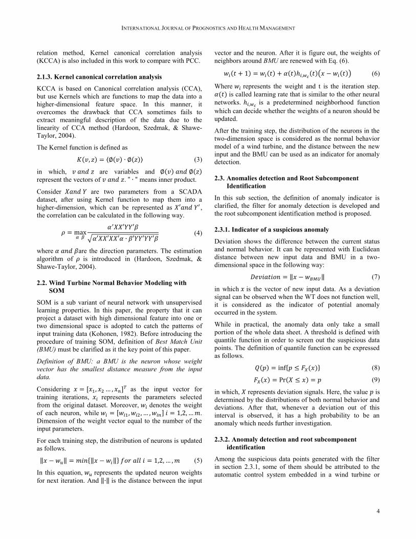
Figure 10. Case 1 WT keeps working when warning signal

hit one

Case 1, wind turbine keeps working when warning signal

hits one. As is shown in Figure 10, the proposed method

tracks the warning signal properly, and can find sharp

increase several periods before the warning signal.

Case 2, from the results generated by SOM, the deviations

from the “normal” behaviors show that some ‘big’ jumps

exist and this should be investigated. As is shown in Figure

11, when ‘big’ jumps occur, all the sub parameters show

exactly same patterns, i.e. a sudden increase around the

warning time. In practical, multi-failure at the same time is

almost impossible and the ratio of each parameter count for

the deviation does not change in this case. What is more,

when check original data, it is almost sure that this ‘big

jump’ case should be attributed to sensor errors.

Case 3 is corresponding to the longest gap mentioned 4.3

which represents a long time shut down for this WT which

is nearly one day. In this case, there may be a real failure

which needs to be fixed or it is just a scheduled maintenance.

Figure 11. Case 2 extreme cases in which deviation values

are too big.

From Figure 12, the deviation signal during this time scale

suddenly increased and suffered vibration in the next several

periods. Hence, there may be an anomaly among the sub

conponents which need further investigation.

Figure 12. Case 3 the longest shut down time in two months

10

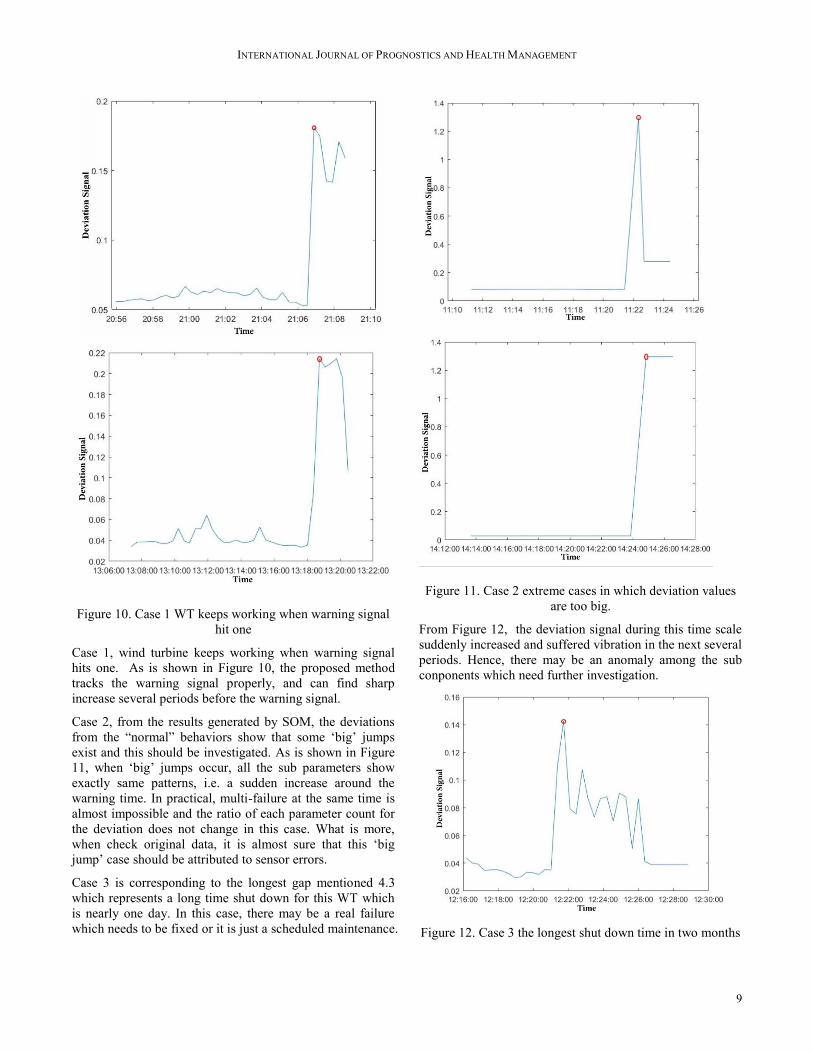
Figure 13. Case 4 WT is shut down after warning signal hits

one

Case 4, is when the value of fault signal hit 1, WT is not

working. In Figure 13, the patterns of the curves do not

show significant differences from case 1. However, when

checking the average value of deviation signals, the average

level in case 4 is higher, which implies that the condition of

the wind turbine is worse than in case 1.

Based on the proposed method, only 5 cases are confirmed

as anomalies after checking the original SCADA data. They

are shown in Figure 10, 12, 13. The SOM based anomaly

detection method is sensitive to the changes of the

parameters. This lead to the cases shown in Figure 11, as

sensor errors can bring interferences. Also for failures

caused by ageing, which often has a relatively long time

process, the remaining life model based failure detection

method is more powerful. But whenever an anomaly occurs

and the corresponding parameters change, the proposed

method can detect it.

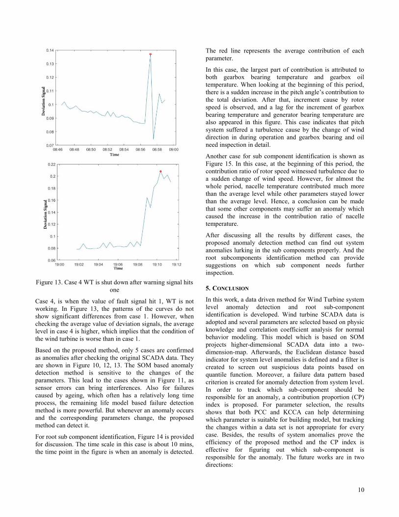
For root sub component identification, Figure 14 is provided

for discussion. The time scale in this case is about 10 mins,

the time point in the figure is when an anomaly is detected.

The red line represents the average contribution of each

parameter.

In this case, the largest part of contribution is attributed to

both gearbox bearing temperature and gearbox oil

temperature. When looking at the beginning of this period,

there is a sudden increase in the pitch angle’s contribution to

the total deviation. After that, increment cause by rotor

speed is observed, and a lag for the increment of gearbox

bearing temperature and generator bearing temperature are

also appeared in this figure. This case indicates that pitch

system suffered a turbulence cause by the change of wind

direction in during operation and gearbox bearing and oil

need inspection in detail.

Another case for sub component identification is shown as

Figure 15. In this case, at the beginning of this period, the

contribution ratio of rotor speed witnessed turbulence due to

a sudden change of wind speed. However, for almost the

whole period, nacelle temperature contributed much more

than the average level while other parameters stayed lower

than the average level. Hence, a conclusion can be made

that some other components may suffer an anomaly which

caused the increase in the contribution ratio of nacelle

temperature.

After discussing all the results by different cases, the

proposed anomaly detection method can find out system

anomalies lurking in the sub components properly. And the

root subcomponents identification method can provide

suggestions on which sub component needs further

inspection.

5. CONCLUSION

In this work, a data driven method for Wind Turbine system

level anomaly detection and root sub-component

identification is developed. Wind turbine SCADA data is

adopted and several parameters are selected based on physic

knowledge and correlation coefficient analysis for normal

behavior modeling. This model which is based on SOM

projects higher-dimensional SCADA data into a two-

dimension-map. Afterwards, the Euclidean distance based

indicator for system level anomalies is defined and a filter is

created to screen out suspicious data points based on

quantile function. Moreover, a failure data pattern based

criterion is created for anomaly detection from system level.

In order to track which sub-component should be

responsible for an anomaly, a contribution proportion (CP)

index is proposed. For parameter selection, the results

shows that both PCC and KCCA can help determining

which parameter is suitable for building model, but tracking

the changes within a data set is not appropriate for every

case. Besides, the results of system anomalies prove the

efficiency of the proposed method and the CP index is

effective for figuring out which sub-component is

responsible for the anomaly. The future works are in two

directions:


11

Figure 14. Root sub component identification case study (abnormal Gearbox)

Figure 15. Root sub component identification case study (abnormal Nacelle temperature)

1. Parameter selection for data driven modeling needs more

investigation. An approach without an assumption on the

relationship between variables is preferred.

2. The cumulative deviation curve shown in Figure 16 can

be considered as wind turbine performance degradation

from a long term perspective because it shows how the

condition of a wind turbine changes in a period. According

to (Snchez-Silva, 2015), degradation can be considered as

the decrease in capacity of an engineered system over time,

as measured by one or more performance indicators. Figure

16 represents the cumulative deviation which is the

performance indicator as it shows a successive process that

the condition of a wind turbine is getting worse. This curve

can be used for remaining useful life estimation and


12

performance & maintenance evaluation which need further

investigation.

Figure 16. Cumulative deviations in two months

REFERENCES

Anderson, D. R., Burnham, K. P., & Thompson, W. L.

(2000). Null hypothesis testing: problems,

prevalence, and an alternative. The journal of

wildlife management, 912-923. Breteler, D., Kaidis, C., Tinga, T., & Loendersloot, R.

(2015). Physics based methodology for wind

turbine failure detection, diagnostics & prognostics.

In EWEA 2015 (pp. 1-9). European Wind Energy

Association.

Bruce, T., Long, H., & Dwyer-Joyce, R. S. (2015). Dynamic

modelling of wind turbine gearbox bearing loading

during transient events. Renewable Power

Generation, IET, 9(7), 821-830.

Castellani, F., Astolfi, D., Sdringola, P., Proietti, S., & Terzi,

L. (2015). Analyzing wind turbine directional

behavior: SCADA data mining techniques for

efficiency and power assessment. Applied Energy.

Chen, B. (2014). Automated On-line Fault Prognosis for

Wind Turbine Monitoring using SCADA data.

Durham University.

de Andrade Vieira, R., & Sanz-Bobi, M. (2013). Failure

Risk Indicators for a Maintenance Model Based on

Observable Life of Industrial Components With an

Application to Wind Turbines. IEEE Transactions

on Reliability, 62(3), 569 - 582.

de Azevedo, H. D., Araújo, A. M., & Bouchonneau, N.

(2016). A review of wind turbine bearing condition

monitoring: State of the art and challenges.

Renewable and Sustainable Energy Reviews, 56,

368-379.

de Bessa, I. V., Palhares, R. M., D'Angelo, M. F., & Chaves

Filho, J. E. (n.d.). Data-driven fault detection and

isolation scheme for a wind turbine benchmark.

Depren, O., Topallar, M., Anarim, E., & Ciliz, M. K. (2005).

An intelligent intrusion detection system (IDS) for

anomaly and misuse detection in computer

networks. Expert systems with Applications, 713-

722.

European Wind Energy Association. (2016). Wind in power

2015 European statistics.

Fabio A, G., & Dipankar, D. (2003). Anomaly Detection

Using Real-Valued Negative Selection. Genetic

Programming and Evolvable Machines, 383-403.

Hardoon, D. R., Szedmak, S., & Shawe-Taylor, J. (2004).

Canonical correlation analysis: An overview with

application to learning methods. Neural

computation, 16(12), 2639-2664.

Hoglund, A. J., Hatonen, K., & Sorvari, A. S. (2000). A

computer host-based user anomaly detection

system using the self-organizing map. In Neural

Networks, 2000. IJCNN 2000, Proceedings of the

IEEE-INNS-ENNS International Joint Conference

on (pp. 411-416).

Kandukuri, S. T., Karimi, H. R., & Robbersmyr, K. G.

(2016). A review of diagnostics and prognostics of

low-speed machinery towards wind turbine farm-

level health management. Renewable and

Sustainable Energy Reviews, 53, 697-708.

Kohonen, T. (1982). Self-organized formation of

topologically correct feature maps. Biological

cybernetics, 59-69.

Lamedica, R., Prudenzi, A., Sforna, M., Caciotta, M., &

Cencellli, V. O. (1996). A neural network based

technique for short-term forecasting of anomalous

load periods. IEEE Transactions on Power Systems,

1749-1756.

Lapira, Edzel, & al, e. (2012). Wind turbine performance

assessment using multi-regime modeling approach.

Renewable Energy(45), 86-95.

Marhadi, K. S., & Skrimpas, G. A. (2015). Automatic

Threshold Setting and Its Uncertainty

Quantification in Wind Turbine Condition

Monitoring System. International Journal of

Prognostics and Health Management,6(Special

Issue Uncertainty in PHM).

Milborrow, D. (2006). Operation and maintenance costs

compared and revealed. Windstats Newsletter, 19,

1-3.

Park, B., Sohn, H., Malinowski, P., & Ostachowicz, W.

(2016). Delamination localization in wind turbine

blades based on adaptive time-of-flight analysis of

noncontact laser ultrasonic signals. Nondestructive

Testing and Evaluation, 1-20.

Rigamonti, M. a., Zio, E., Alessi, A., Astigarraga, D., &

Galarza, A. (2015). A Self-Organizing Map-Based

Monitoring System for Insulated Gate Bipolar


13

Transistors Operating in Fully Electric Vehicle.

Annual Conference of the Prognostic and Health

Management Society 2015.

Santos, P., Villa, L. F., Reñones, A., Bustillo, A., & Maudes,

J. (2015). An SVM-based solution for fault

detection in wind turbines. Sensors, 15(3), 5627-

5648.

Schlechtingen, M., Santos, I. F., & Achiche, S. (2013).

Wind turbine condition monitoring based on

SCADA data using normal behavior models. Part 1:

System description. Applied Soft Computing, 13(1),

259-270.

Snchez-Silva, M. (2015). Degradation: Data Analysis and

Analytical Modeling. In Reliability and Life-Cycle

Analysis of Deteriorating System (pp. 79-82).

Springer.

Sun, P., Li, J., Wang, C., & Lei, X. (2016). A generalized

model for wind turbine anomaly identification

based on SCADA data. Applied Energy, 168, 550-

567.

Tian, J., Azarian, M. H., & Pecht, M. (2014). Anomaly

Detection Using Self-Organizing Maps-Based K-

Nearest Neighbor Algorithm. Proceedings of the

European Conference of the Prognostics and

Health Management Society. Citeseer.

Vesanto, J., Himberg, J., Alhoniemi, E., & Parhankangas, J.

(2000). SOM toolbox for Matlab 5. Helsinki,

Finland: Helsinki University of Technology.

Wilkinson, M., Darnell, B., Delft, T. V., & Harman, K.

(2014). Comparison of methods for wind turbine

condition monitoring with SCADA data. IET

Renewable Power Generation, 390-397.

Xiang, J., Watson, S., & Liu, Y. (2009). Smart monitoring

of wind turbines using neural networks. In

Sustainability in Energy and Buildings (pp. 1-8).

Springer.

Yang, D., Li, H., Hu, Y., Zhao, J., Xiao, H., & Lan, Y.

(2016). Vibration condition monitoring system for

wind turbine bearings based on noise suppression

with multi-point data fusion. Renewable Energy,

92, 104-116.

Zhao, W., Siegel, D., Lee, J., & Su, L. (2013). An integrated

framework of drivetrain degradation assessment

and fault localization for offshore wind turbines.

IJPHM Special Issue on Wind Turbine PHM

(Color), 46-58.

Zhong, B., Wang, J., Wu, H., Zhou, J., & Jin, Q. (2016).

SOM-based visualization monitoring and fault

diagnosis for chemical process. 2016 Chinese

Control and Decision Conference (CCDC), (pp.

5844-5849).

A SOM based Anomaly Detection Method for Wind … Journal of Prognostics and Health Management, ISSN...

Documents

Transcript of A SOM based Anomaly Detection Method for Wind … Journal of Prognostics and Health Management, ISSN...