
A solution to the dynamical inverse problem of EEG...
19
A solution to the dynamical inverse problem of EEG generation using spatiotemporal Kalman filtering Andreas Galka, a,b, * Okito Yamashita, c Tohru Ozaki, b,c Rolando Biscay, d and Pedro Valde ´s-Sosa e a Institute of Experimental and Applied Physics, University of Kiel, 24098 Kiel, Germany b Institute of Statistical Mathematics (ISM), Tokyo 106-8569, Japan c Department of Statistical Science, The Graduate University for Advanced Studies, Tokyo 106-8569, Japan d University of Havana, Havana, Cuba e Cuban Neuroscience Center, Havana, Cuba Received 28 July 2003; revised 27 January 2004; accepted 12 February 2004 Available online 8 August 2004 We present a new approach for estimating solutions of the dynamical inverse problem of EEG generation. In contrast to previous approaches, we reinterpret this problem as a filtering problem in a state space framework; for the purpose of its solution, we propose a new extension of Kalman filtering to the case of spatiotemporal dynamics. The temporal evolution of the distributed generators of the EEG can be reconstructed at each voxel of a discretisation of the gray matter of brain. By fitting linear autoregressive models with neighbourhood interactions to EEG time series, new classes of inverse solutions with improved resolution and localisation ability can be explored. For the purposes of model comparison and parameter estimation from given data, we employ a likelihood maximisation approach. Both for instantaneous and dynamical inverse solutions, we derive estimators of the time-dependent estimation error at each voxel. The performance of the algorithm is demonstrated by application to simulated and clinical EEG recordings. It is shown that by choosing appropriate dynamical models, it becomes possible to obtain inverse solutions of considerably improved quality, as compared to the usual instantaneous inverse solutions. D 2004 Elsevier Inc. All rights reserved. Keywords: EEG; Inverse problem; Kalman filtering; Whitening; Spatio- temporal modeling; AIC; Maximum likelihood Introduction Recordings of electromagnetic fields emanating from human brain are well known to provide an important source of information about brain dynamics. Electrical potentials on the scalp surface are very easy to measure at a set of electrodes attached to the skin; as a result, multivariate electroencephalographic (EEG) time series are obtained. With considerably higher technical effort, magnetoence- phalographic (MEG) time series can also be recorded. It is by now widely accepted that the sources of these electro- magnetic fields are electrical currents within networks of neurons in the cortex and other gray matter structures of brain; while part of this current remains confined within the dendritic trunks (primary currents), another part flows through the extracellular volume (secondary currents) (Nunez, 1981). To obtain more direct access to the dynamics governing the activity of these networks of neurons, it would be desirable to have direct estimates of these sources. The estimation of these sources from recordings of EEG or MEG has recently become a subject of intense research (Darvas et al., 2001; Gorodnitsky et al., 1995; Grave de Peralta Menendez and Gonzalez Andino, 1999; Greenblatt, 1993; Pascual-Marqui et al., 1994; Phillips et al., 2002; Riera et al., 1998; Scherg and Ebersole, 1994; Schmitt et al., 2002; Yamashita et al., 2004; for a recent review see Baillet et al., 2001). In this paper, we focus on the case of the EEG, but the ideas and methods to be presented remain equally valid for the MEG. Two main classes of source models have been developed: ‘‘equivalent current dipole’’ approaches (also known as ‘‘paramet- ric’’ methods), in which the sources are modeled by a relatively small number of focal sources at locations to be estimated from the data, and ‘‘linear distributed’’ approaches (also known as ‘‘imag- ing’’ or ‘‘current density reconstruction’’ methods), in which the sources are modeled by a dense set of dipoles distributed at fixed locations (which, in analogy to the case of magnetic resonance imaging, we shall call ‘‘voxels’’) throughout the head volume. Examples of parametric approaches include least-squares source estimation (Scherg and Ebersole, 1994) and spatial filters, such as beamforming and multiple signal classification (‘‘MUSIC’’) approaches (Mosher et al., 1992). This paper exclusively deals with the linearly distributed model approach. It is a characteristic problem of distributed source models that a large number of unknown quantities has to be estimated from a much smaller number of measurements; because of this, we are facing a problem that does not possess a unique solution, known as ‘‘inverse problem’’. The number of measurements given at one instant of time may be as low as 18, if the standard 10–20 system of clinical EEG recordings is employed; by increasing the number of electrodes, we may eventually obtain up to a few hundred 1053-8119/$ - see front matter D 2004 Elsevier Inc. All rights reserved. doi:10.1016/j.neuroimage.2004.02.022 * Corresponding author. Institute of Statistical Mathematics (ISM), Minami-Azabu 4-6-7, Minato, Tokyo 106-8569, Japan. Fax: +81-3-3446- 8751. E-mail address: [email protected] (A. Galka). Available online on ScienceDirect (www.sciencedirect.com.) www.elsevier.com/locate/ynimg NeuroImage 23 (2004) 435 – 453
Transcript of A solution to the dynamical inverse problem of EEG...
www.elsevier.com/locate/ynimg
NeuroImage 23 (2004) 435–453
A solution to the dynamical inverse problem of EEG generation using
spatiotemporal Kalman filtering
Andreas Galka,a,b,* Okito Yamashita,c Tohru Ozaki,b,c Rolando Biscay,d and Pedro Valdes-Sosae
a Institute of Experimental and Applied Physics, University of Kiel, 24098 Kiel, Germanyb Institute of Statistical Mathematics (ISM), Tokyo 106-8569, JapancDepartment of Statistical Science, The Graduate University for Advanced Studies, Tokyo 106-8569, JapandUniversity of Havana, Havana, CubaeCuban Neuroscience Center, Havana, Cuba
Received 28 July 2003; revised 27 January 2004; accepted 12 February 2004
Available online 8 August 2004
We present a new approach for estimating solutions of the dynamical
inverse problem of EEG generation. In contrast to previous
approaches, we reinterpret this problem as a filtering problem in a
state space framework; for the purpose of its solution, we propose a
new extension of Kalman filtering to the case of spatiotemporal
dynamics. The temporal evolution of the distributed generators of the
EEG can be reconstructed at each voxel of a discretisation of the gray
matter of brain. By fitting linear autoregressive models with
neighbourhood interactions to EEG time series, new classes of inverse
solutions with improved resolution and localisation ability can be
explored. For the purposes of model comparison and parameter
estimation from given data, we employ a likelihood maximisation
approach. Both for instantaneous and dynamical inverse solutions, we
derive estimators of the time-dependent estimation error at each voxel.
The performance of the algorithm is demonstrated by application to
simulated and clinical EEG recordings. It is shown that by choosing
appropriate dynamical models, it becomes possible to obtain inverse
solutions of considerably improved quality, as compared to the usual
instantaneous inverse solutions.
D 2004 Elsevier Inc. All rights reserved.
Keywords: EEG; Inverse problem; Kalman filtering; Whitening; Spatio-
temporal modeling; AIC; Maximum likelihood
Introduction
Recordings of electromagnetic fields emanating from human
brain are well known to provide an important source of information
about brain dynamics. Electrical potentials on the scalp surface are
very easy to measure at a set of electrodes attached to the skin; as a
result, multivariate electroencephalographic (EEG) time series are
obtained. With considerably higher technical effort, magnetoence-
phalographic (MEG) time series can also be recorded.
1053-8119/$ - see front matter D 2004 Elsevier Inc. All rights reserved.
doi:10.1016/j.neuroimage.2004.02.022
* Corresponding author. Institute of Statistical Mathematics (ISM),
Minami-Azabu 4-6-7, Minato, Tokyo 106-8569, Japan. Fax: +81-3-3446-
8751.
E-mail address: [email protected] (A. Galka).
Available online on ScienceDirect (www.sciencedirect.com.)
It is by now widely accepted that the sources of these electro-
magnetic fields are electrical currents within networks of neurons
in the cortex and other gray matter structures of brain; while part of
this current remains confined within the dendritic trunks (primary
currents), another part flows through the extracellular volume
(secondary currents) (Nunez, 1981). To obtain more direct access
to the dynamics governing the activity of these networks of
neurons, it would be desirable to have direct estimates of these
sources. The estimation of these sources from recordings of EEG
or MEG has recently become a subject of intense research (Darvas
et al., 2001; Gorodnitsky et al., 1995; Grave de Peralta Menendez
and Gonzalez Andino, 1999; Greenblatt, 1993; Pascual-Marqui et
al., 1994; Phillips et al., 2002; Riera et al., 1998; Scherg and
Ebersole, 1994; Schmitt et al., 2002; Yamashita et al., 2004; for a
recent review see Baillet et al., 2001). In this paper, we focus on
the case of the EEG, but the ideas and methods to be presented
remain equally valid for the MEG.
Two main classes of source models have been developed:
‘‘equivalent current dipole’’ approaches (also known as ‘‘paramet-
ric’’ methods), in which the sources are modeled by a relatively
small number of focal sources at locations to be estimated from the
data, and ‘‘linear distributed’’ approaches (also known as ‘‘imag-
ing’’ or ‘‘current density reconstruction’’ methods), in which the
sources are modeled by a dense set of dipoles distributed at fixed
locations (which, in analogy to the case of magnetic resonance
imaging, we shall call ‘‘voxels’’) throughout the head volume.
Examples of parametric approaches include least-squares source
estimation (Scherg and Ebersole, 1994) and spatial filters, such as
beamforming and multiple signal classification (‘‘MUSIC’’)
approaches (Mosher et al., 1992). This paper exclusively deals
with the linearly distributed model approach.
It is a characteristic problem of distributed source models that a
large number of unknown quantities has to be estimated from a
much smaller number of measurements; because of this, we are
facing a problem that does not possess a unique solution, known as
‘‘inverse problem’’. The number of measurements given at one
instant of time may be as low as 18, if the standard 10–20 system
of clinical EEG recordings is employed; by increasing the number
of electrodes, we may eventually obtain up to a few hundred
A. Galka et al. / NeuroImage 23 (2004) 435–453436
measurements, but they will fail to provide an equivalent amount
of independent information due to strong correlations between
adjacent electrodes. On the other hand, the number of voxels will
typically be several thousand, and furthermore at each voxel site a
full three-dimensional current vector has to be modelled.
To identify a unique solution (i.e., an ‘‘inverse solution’’),
additional information has to be employed. So far this has been
donemainly by imposing constraints on the inverse solution. Certain
constraints can be obtained from neurophysiology (Phillips et al.,
2002); as an example, it is reasonable to assume that only voxels
within gray matter contribute substantially to the generation of the
electromagnetic fields; other constraints refer to the probable direc-
tion of local current vectors at specific locations. But such constraints
do not suffice to remove the ambiguity of the inverse solution.
For this purpose, much more restrictive constraints are needed,
such as the minimum-norm constraint suggested by Hamalainen
and Ilmoniemi (1984) or the maximum-smoothness constraint
suggested by Pascual-Marqui et al. (1994). These constraints can
be applied independently for each instant of time, without access-
ing the data measured at other instants of time; therefore, we will
say that the resulting inverse solutions represent solutions of the
‘‘instantaneous’’ inverse problem.
The idea of including data from more than a single instant of
time into the estimation of inverse solutions is attractive, since
more information becomes available for the solution of an ill-posed
problem; consequently, there has recently been growing interest in
generalising the instantaneous inverse problem to ‘‘dynamical’’
inverse problems and to develop algorithms for its solution (Darvas
et al., 2001; Kaipio et al., 1999; Schmitt et al., 2002; Somersalo et
al., 2003).
In this paper, we will contribute to these efforts by developing a
new interpretation of the dynamic inverse problem in its most
general shape, and by proposing a new approach to its solution. In
contrast to most previous work, we will not approach this problem
within a constrained least squares (or, equivalently, Bayesian)
framework, but by reformulating it as a spatiotemporal state space
filtering problem. So far, the dynamical aspect of the available
algorithms was essentially limited to imposing temporal smooth-
ness constraints (Baillet and Garnero, 1997; Schmitt et al., 2002);
from a time-domain modelling perspective, such constraints cor-
respond to the very special case of a spatially noncoupled random-
walk model (Somersalo et al., 2003). By appropriate generalisa-
tion, our approach will permit the use of much more general
predictive models in this context, such that a consistent description
of the spatiotemporal dynamics of brain becomes possible.
It should be stressed that general predictive models can also be
incorporated into the framework of constrained least squares, and
in a companion paper to this paper we will discuss in more detail
the application of this idea to the inverse problem of EEG
generation (Yamashita et al., 2004).
As the main tool for our task, we will adapt the well-known
Kalman filter (Chui and Chen, 1999) to spatiotemporal filtering
problems; it will become evident that Kalman filtering provides a
natural framework for addressing the dynamical inverse problem of
EEG generation. Theoretically, by employing a very high-dimen-
sional state vector, standard Kalman filtering could deal with any
spatiotemporal filtering problem, but the specific nature of the
spatial dimensions (such as neighbourhood relationships between
voxels) would not be properly captured, and computational
expenses would soon become prohibitively large. By assuming a
properly chosen structure of the dynamics and certain additional
approximations, the intractable high-dimensional filtering problem
can be decomposed into a coupled set of tractable low-dimensional
filtering problems. This adaptation can be regarded as a general-
isation of standard Kalman filtering to the case of partial (space–
time) differential equations.
From system theory, it is known that the sufficient condition for
successful application of Kalman filtering is observability of the
given state space system, as represented by its state transition
parameter matrix (or, in the nonlinear case, the corresponding
Jacobian matrix) and its observation matrix (Kailath, 1980; Kal-
man et al., 1969). Although we will not be able to rigorously prove
observability, we will discuss the application of this concept to our
model and demonstrate through an explicit numerical simulation
study that Kalman filtering can successfully be applied. From this
simulation, it will also become evident that a crucial element for
the estimation of dynamical inverse solutions is given by the model
according to which the dynamics of the voxel currents is assumed
to evolve. If a very simple model is chosen, we will obtain
solutions that offer only small improvements over solutions result-
ing from previous nondynamical (i.e., instantaneous) algorithms
for solving the inverse problem; if the model contains additional
information about the true dynamics, much better solutions can be
obtained. Such information can at least partly be obtained by
choosing a model with a sufficient flexibility for adaptation to
given data; this adaptation can be performed by suitable fitting of
dynamical parameters and noise covariances.
We will propose to employ the maximum likelihood method for
this fitting task; it will become evident that Kalman filtering is the
natural tool for calculating the likelihood from EEG data. By
assuming a somewhat more general viewpoint, we will address
parameter estimation as a special case of model comparison, and
employ appropriate statistical criteria, namely the Akaike Informa-
tion Criterion (AIC) and its Bayesian variant, ABIC, for the
purpose of comparing inverse solutions. Numerical examples will
be shown both for simulated data and for a clinical EEG recording.
Finally, it should be mentioned that there exists already a
sizable amount of published work dealing with applications of
Kalman filtering to the analysis of EEG recordings, which we are
unable to review in any appropriate form in this paper; and
furthermore there exist also applications of Kalman filtering, or
related filtering approaches, to inverse problems, some of which
also fall into the field of biomedical data analysis, like Electrical
Impedance Tomography or evoked potential estimation (see, e.g.,
Baroudi et al., 1998; Kaipio et al., 1999; Karjalainen, 1997).
Recently, Somersalo et al. (2003) have applied a nonlinear alter-
native to Kalman filtering, known as particle filtering, to the
problem of estimating focal sources from MEG data. While
providing important results and methodology, so far none of these
studies has addressed the problem of reconstruction of distributed
sources from EEG (or MEG) times series in the context of
identification of optimal dynamical (i.e., predictive) models.
In this paper, we will introduce a new practicable solution for
the problem of applying Kalman filtering to very high dimensional
filtering problems, as they arise in the case of spatiotemporal brain
dynamics. Moreover, we will replace the largely arbitrary choice of
dynamical models that can be seen in many applications of Kalman
filtering, by a systematic model comparison and selection approach
that provides explicit justification for the chosen model and
parameters in terms of the numerical value of a statistical criterion.
By this approach, a wide class of very general models becomes
available for data-driven modelling of brain dynamics.
A. Galka et al. / NeuroImage 23 (2004) 435–453 437
The inverse problem of EEG generation
We start from a rectangular grid of Nv voxels covering the
cortical gray matter parts of human brain; in this study, inverse
solutions will be confined to these voxels. In the particular discre-
tisation that we will employ, there are Nv = 3433 cortical gray-matter
voxels. At each voxel, a local three-dimensional current vector
jðv; tÞ ¼ ðjxðv; tÞ; jyðv; tÞ; jzðv; tÞÞy
is assumed, where v is a voxel label, t denotes time, and y denotesmatrix transposition. The column vector of all current vectors (i.e.,
for all gray-matter voxels) will be denoted by
JðtÞ ¼ ðjð1; tÞy; jð2; tÞy; . . . ; jðNv; tÞyÞy
which represents the dynamical state variable of the entire system.
These currents are mapped to the electroencephalographic
signal (EEG), which is recorded at the scalp surface. The EEG at
an individual electrode shall be denoted by y(i,t), where i is an
electrode label; the nc-dimensional column vector composed of all
the electric potentials at all available electrodes shall be denoted by
YðtÞ ¼ ðyð1; tÞ; yð2; tÞ; . . . ; yðnc; tÞÞy
In this study, we assume that the 10–20 system is employed; all
potentials refer to average reference, although other choices are
possible. Due to the choice of a reference out of the set of
electrodes, it is advisable to exclude one of the standard electrodes
of the 10–20 system from further analysis, such that the effective
dimension of Y becomes nc = 18.
For distributed source models, it is possible to approximate the
mapping from J to Y by a linear function (Baillet et al., 2001)
whence it can be expressed as
YðtÞ ¼ KJðtÞ þ :ðtÞ ð1Þ
Here K denotes a nc � 3Nv transfer matrix, commonly called ‘‘lead
field matrix’’. This matrix can approximately be calculated for a
three-shell head model and given electrode locations by the
‘‘boundary element method’’ (Ary et al., 1981; Buchner et al.,
1997; Pascual-Marqui et al., 1994; Riera et al., 1998). It is an
essential precondition for any approach to find inverse solutions
that a reliable estimate of this matrix is available. Here we remark
that typically the lead field matrix turns out to be of full rank.
It will be convenient for later use to define the individual
contribution of each voxel to the vector of observations by
K(v)j(v,t), where K(v) is the nc � 3 matrix that results from
extracting those three columns out of K, which are multiplied with
j(v,t) in the process of the multiplication of K and J(t). From this
definition, Eq. (1) can also be written as
YðtÞ ¼XNv
v¼1
KðvÞjðv; tÞ þ :ðtÞ ð2Þ
By : (t), we denote a vector of observational noise, which we
assume to be white and Gaussian with zero mean and covariance
matrix Ce = E(:: y). We will make the assumption that Ce has the
simplest possible structure, namely
Ce ¼ r2e Inc ð3Þ
where Inc denotes the nc � nc identity matrix; that is, we assume
that the observation noise is uncorrelated between all pairs of
electrodes and of equal variance for all electrodes. These assump-
tions may be relaxed in future work.
Eq. (1) is part of the standard formulation of the inverse
problem of EEG (Pascual-Marqui, 1999); in this paper, we propose
to interpret it as an observation equation in the framework of
dynamical state-space modelling.
The inverse problem of EEG generation is given by the problem
of estimating the generators J(t) from the observed EEG Y(t); this
obviously constitutes an ill-posed problem since the dimension of
J(t) is much larger than the dimension of Y(t). As also in the case
of many other inverse problems, it is nevertheless possible to
obtain approximate estimates of J(t). As a representative of the
numerous approaches that have been proposed for this purpose, we
select here the ‘‘low-resolution brain electromagnetic tomography’’
(LORETA) algorithm, proposed by Pascual-Marqui et al. (1994),
as a starting point; a brief introduction will be given in the next
section.
The instantaneous case
The LORETA approach
In this approach, a spatial smoothness constraint is imposed on
the estimate of J(t), which can be expressed by employing a
discrete spatial Laplacian operator defined by
L ¼ INv� 1
6N
� �� I3 ð4Þ
Here N denotes a Nv � Nv matrix having Nvv V = 1 if v V belongs tothe set of neighbours of voxel v [this set shall be denoted byNðvÞ],and 0 otherwise. By the symbol �, Kronecker multiplication of
matrices is denoted. The (3i)th row vector of L acts as a discrete
differentiating operator by forming differences between the nearest
neighbours of the ith voxel and ith voxel itself (with respect to the
first vector component).
In the LORETA approach, the inverse solution is obtained by
minimizing the objective function
EðJÞ ¼ NðY � KJÞN2 þ k2NLJN2 ð5Þ
i.e., a weighted sum of the observation fitting error and of a term
measuring nonsmoothness by the norm of the spatial Laplacian of
the state vector. ||.|| denotes Euclidean norm. The hyperparameter kexpresses the balance between fitting of observations and the
smoothness constraint; a nonzero value for k provides regularisa-
tion for the solution (Hofmann, 1986).
Here we would like to mention that the second term in Eq. (5)
represents a special example of a general constraint term; by
appropriate choice of this term, it is also possible to impose other
kinds of constraints instead of spatial smoothness, such as ana-
tomical constraints or sparseness of the inverse solution (see Baillet
et al., 2001, and references cited therein).
The least squares solution of the problem of minimising Eq. (5)
is given by
J ¼ ðKyK þ k2LyLÞ�1KyY ð6Þ
here by J the estimator of the state vector J is denoted. Within the
framework of Bayesian inference, this solution can be interpreted
A. Galka et al. / NeuroImage 23 (2004) 435–453438
as the Maximum A Posteriori (MAP) solution for the case of
Gaussian distributions for the likelihood and the prior (Tarantola,
1987; Yamashita et al., 2004):
pðY j J; r2eÞfNðKJ; r2
eÞ
pðJ; s2ÞfNð0; s2ðLyLÞ�1Þ ð7Þ
where we have defined s = re/k.Note that J will not depend on the reference according to which
the EEG data Y was measured; this dependence is absorbed into the
lead-field matrix. This effect represents another advantage of
transforming EEG data into an estimated source current density:
the notorious reference problem of EEG is completely removed by
this transformation.
The matrix KyK þ k2LyL in Eq. (6) has the size 3Nv � 3Nv c104 � 104, whence actual numerical inversion is usually imprac-
ticable. The solution can be evaluated nevertheless by using the
singular value decomposition of the nc � 3Nv matrix KL�1,
KL�1 ¼ USVy ð8Þ
where U is an orthogonal nc � nc matrix, S is a nc � 3Nv
matrix whose only nonzero elements are the singular values
Siiusi; i ¼ 1; . . . ; nc , and V is an orthogonal 3Nv � 3Nv matrix;
only the first nc columns of V are relevant for this decomposition,
and the corresponding 3Nv � nc matrix shall be denoted by Vð1Þ.The matrix composed of the remaining 3Nv � nc columns shall be
denoted by Vð2Þ. After some transformations, Eq. (6) becomes
J ¼ L�1Vð1Þdiagsi
s2i þ k2
!UyY ð9Þ
Here diag (xi) denotes a diagonal matrix with elements x1,. . .,xnc on
its diagonal. Numerical evaluation of this expression can be
implemented very efficiently.
Estimation of the regularisation parameter k
Since the inverse solution given by Eq. (9) will depend
sensitively on the value of the hyperparameter k, it should be
chosen in an objective way. Various statistical criteria, such as
Generalised Cross-Validation (GCV) (Wahba, 1990), and ad hoc
methods, such as the L-curve approach (Lawson and Hanson,
1974), have been employed for this purpose. Instead of these
approaches, in this paper, we have chosen to use the Akaike
Bayesian Information Criterion (ABIC) (Akaike, 1980a,b), since
we intend to directly compare inverse solutions obtained by
different techniques by comparing their likelihood.
Given a time series of EEG observations Y(1),. . .,Y(Nt), ABIC
is defined as (�2) times the type II log-likelihood; that is, the log-
likelihood of the hyperparameters in the context of empirical
Bayesian inference. In the case of the model containing unobserv-
able variables, the type II likelihood can be obtained by averaging
the joint distribution of all variables, both observable and unob-
servable, over the unobservable variables, i.e., by forming the
marginal distribution:
ABICðre; sÞ ¼ �2logLIIðre; sÞ
¼ �2XNt
t¼1
log
ZpðYðtÞjJðtÞ; r2
eÞpðJðtÞ; s2ÞdJðtÞ
ð10Þ
where Y(t) are the observable and J(t) the unobservable variables;
re, s are hyperparameters, and again s = re/k.Estimators for re and k can be obtained by maximising the
likelihood given by Eq. (10); how this can be done in an efficient
way will be presented elsewhere in more detail (Yamashita et al.,
2004). Here we give only the result.
The type II log-likelihood LII(re, s) itself can be shown to be
LIIðre; kÞ ¼XNt
t¼1
Xnci¼1
logs2i þ k2
k2þ ncð1þ log2pr2
eÞ !
ð11Þ
where the estimate of the observation noise variance re2 is given by
r2e ¼
1
nc
Xnci¼1
k2
s2i þ k2y2iðtÞ ð12Þ
here yi(t) denotes the ith element of the vector UyYðtÞ, where U is
defined in Eq. (8).
As a result, we obtain not only estimates for the hyperpara-
meters, but also the possibility to calculate the ABIC value for any
given inverse solution (as obtained by LORETA), i.e., an estimate
for the type II likelihood. This will enable us to compare inverse
solutions obtained by different techniques, since for given data the
likelihood serves as a general measure of the quality of hypotheses
(Akaike, 1985).
It should be mentioned here that despite using an improved
statistical criterion, the proper choice of the regularisation parameter
remains a difficult problem of the LORETA method; in practice,
frequently even the order of magnitude of the appropriate value of kis debatable and may change drastically upon seemingly insignifi-
cant changes of the data. Also for this reason, there is a growing need
for an alternative approach to estimating inverse solutions.
Estimation of the covariance matrix of the estimated state vector
So far, the lack of an efficient method for assessing the approx-
imate error associated with the inverse solutions obtained by
LORETA has been a serious weakness of this technique; certainly,
it has contributed much to the widespread scepticism that the very
idea of estimating solutions for the inverse problem of EEG
generation is still facing. Strictly speaking, estimates of unobserv-
able quantities without estimates of the corresponding error have to
be regarded as meaningless. For this reason, we introduce a method
for estimating the covariance matrix CðiISÞJ
of the estimated currents
JðtÞ of an inverse solution obtained by LORETA (here the super-
script (iIS) denotes ‘‘instantaneous inverse solution’’).
The derivation of the expression for CðiISÞJ
is inspired by recent
work by Pascual-Marqui (2002); the result is given by
CðiISÞJ
¼ s2L�1Vð1Þdiags2i
s2i þ k2
!Vð1ÞyðLyÞ�1 ð13Þ
The detailed derivation is demonstrated in Appendix A.
Through this expression, it becomes possible to display error
estimates for each voxel (and each vector component) individually.
Since a corresponding error estimate can also be computed for the
new dynamical technique for estimating inverse solutions, which
we will introduce in this paper, another quantitative measure for the
comparison of different techniques for estimating inverse solutions
becomes available.
A. Galka et al. / NeuroImage 23 (2004) 435–453 439
The dynamical case
Dynamical models of voxel currents
After discussing various aspects of the LORETA method, we
shall now proceed to the formulation of the new approach for
solving the dynamical inverse problem of EEG generation; it has
already been mentioned that for this purpose an additional
temporal smoothness constraint could be introduced into Eq. (5)
(Baillet and Garnero, 1997; Schmitt et al., 2002). While this
approach will be pursued and extended elsewhere (Yamashita et
al., 2004), here the central concept of our approach will be a new
adaptation of Kalman filtering to the case of spatiotemporal
dynamics.
The Kalman filter provides the optimum tool for predicting,
filtering and smoothing estimates of the state of dynamical
systems that cannot be observed directly, but only through an
observation equation containing observational noise (Chui and
Chen, 1999). As a presupposition for its application, both the
equations governing the dynamics and the observation equation
have to be known.
Since for the case of the dynamics of human brain, no well-
substantiated models for the spatiotemporal dynamics are known
yet, we are faced with the problem of estimating suitable models
from data. Clearly, this constitutes a research task of enormous
complexity that reaches far beyond the scope of this paper;
therefore we will only be able to explore the very first and simplest
approximations to such models.
Having defined a spatial discretisation by using a finite set of
voxels, it is advisable to formulate dynamical models also with
temporal discretisation; for simplicity, we shall regard the basic
time unit of this discretisation as equal to the sampling rate of the
EEG recording. The corresponding time points will be labeled by
t = 1,2,3,. . .,Nt.
In general form, the dynamics of a set of Nv voxels may be
described by nonlinear multivariate autoregressions given as
JðtÞ ¼ FðJðt � 1Þ; Jðt � 2Þ; . . . ; Jðt � pÞ j JÞ þ hðtÞ ð14Þ
where p denotes the positive integer model order and h(t) denotesdynamical noise, which we assume to be white and Gaussian with
zero mean and covariance matrix Cg ¼ EðhhyÞ. When fitting such
models to given data, h(t) represents a time series of innovations,
i.e., components of the data that cannot be explained from the
dynamics itself. It is the aim of modelling to find dynamical
models that produce a Gaussian white innovation time series, such
that the process of modelling can be regarded as ‘‘temporal
whitening’’.
F denotes a function describing the deterministic part of the
dynamics; it may depend on a vector of parameters J. This functionmay contain considerable internal complexity and a huge number
of parameters (described by J), since it maps an input space of
dimensionality 3Nvp to an output space of dimensionality 3Nv.
The simplest nontrivial example of the class of autoregressions
described by Eq. (14) is a linear multivariate autoregressive model
of first order (AR(1)):
JðtÞ ¼ AJðt � 1Þ þ hðtÞ ð15Þ
and here we note that the popular random-walk model is a special
case of this model, with A ¼ I3Nv. The parameter matrix A is of size
(3Nv) � (3Nv), which in our case is of the order of 108. This large
number of parameters is still far too high to be estimated from real
data; therefore we need additional reductions of model complexity.
Also, the practical application of Kalman filtering requires a
simplified model structure.
It is an arguably reasonable assumption that at short time scales,
the dynamics will be restricted to local neighbourhoods; that is,
each voxel will interact only with its direct spatial neighbours; in a
rectangular grid of voxels, there will be six direct neighbours for
each voxel, except for those at the boundaries of the gray-matter
parts of brain. Most elements of A become zero by this proposition.
The dynamical model for each voxel becomes
jðv; tÞ ¼ A1 jðv; t � 1Þ þ 1
6B1
Xv VaNðvÞ
jðv V; t � 1Þ þ hðtÞ ð16Þ
where A1 and B1 now are the autoregressive parameter matrices (of
size 3 � 3) for self-interaction and nearest-neighbour interaction,
respectively, and NðvÞ denotes the set of labels of gray-matter
voxels that are direct neighbours of voxel v. If furthermore we
assume the absence of any interactions between the three projec-
tions of local current vectors (both within and between voxels) and
total spatial homogeneity and isotropy for all pairs of neighbouring
voxels (this assumption extending to the three vector projections as
well), we can ultimately reduce the number of parameters to two.
The dynamical model for each voxel becomes
jðv; tÞ ¼ a1I3 jðv; t � 1Þ þ b1
6I3X
vVaNðvÞjðvV; t � 1Þ þ hðtÞ ð17Þ
where I3 denotes the 3 � 3 identity matrix; now a1 and b1 are scalar
autoregressive parameters. This model implements complete sym-
metry between voxels and also between projections of local
currents; but clearly, this symmetry is not preserved by multipli-
cation with the lead field matrix K . As a consequence of this,
inverse solutions also will display nonsymmetric behaviour with
respect to voxels and projections.
The additional assumptions that are required to define the
simplest possible nontrivial dynamical model, given by Eq. (17),
are almost certainly without physiological justification, but never-
theless this oversimplification is necessary to design a tractable
algorithm as a starting point. As the next step, it becomes possible
again to consider generalisations, such as higher model order,
nonlinearities, or inhomogeneities; as a consequence, it may
become possible to describe more structure present in the data
by the dynamical model and to relegate less power from the data to
the time series of innovations h(t). Here the aim is that the values
in h(t) be as small as possible, contain as little correlation as
possible (i.e., being white noise) and have a distribution as close as
possible to a Gaussian.
As long as only nearest-neighbour interactions are allowed and
a high degree of spatial homogeneity and isotropy is maintained,
the number of unknown parameters can be kept small, and the
problem remains accessible for spatiotemporal Kalman filtering.
By increasing the model order to p, it becomes possible to
describe stochastic oscillations that may be present in the data;
although this case represents a generalisation of Eq. (15), it can
be incorporated into this equation by replacing the order-1 state
vector J(t) by ðJðtÞy; Jðt � 1Þy; . . . ; Jðt � pþ 1ÞyÞy , such that
formally the dynamics remains a linear autoregression of first
order.
A. Galka et al. / NeuroImage 23 (2004) 435–453440
Eq. (17) can alternatively be written as
jðv; tÞ ¼ ða1 þ b1ÞI3 jðv; t � 1Þ
þ b1I31
6
XvVaNðvÞ
jðvV; t � 1Þ
0@
1A� jðv; t � 1Þ
0@
1Aþ hðtÞ
ð18Þ
This equation shows more clearly that the dynamics at each voxel
is composed of two contributions, the first representing the
autoregressive dynamics of the voxel itself and the second repre-
senting small exogenous disturbances that partly are described as
pure noise and partly as the difference between the average of the
states of the neighbouring voxels and the state of the voxel itself.
The latter difference is the same as also used in the Hjorth source
derivation (Hjorth, 1980), but here we employ it directly in the
(three-dimensional) generator space (i.e., the voxel space) instead
of the (two-dimensional) electrode space.
From Eq. (18), it can be seen that our model corresponds to a
specific choice for the parameter matrixA, which can be expressed as
A ¼ ða1 þ b1ÞI3Nv� b1L ð19Þ
where L is the discrete spatial Laplacian operator defined in Eq. (4).
This relation will become useful in the next section.
Finally, we would like to mention that there exists the possibility
of a direct generalisation of Eq. (18) to partial differential equation
models for the description of brain dynamics in continuous time
and space; recently, such models have been explored by various
authors (Jirsa et al., 2002; Robinson et al., 1997). In the continuous
case (with respect to both time and space), the second term on the
rhs of Eq. (18) (i.e., the term corresponding to the Laplacian)
becomes a second derivative with respect to space, while the two
terms jðv; tÞ � ða1 þ b1ÞI3 jðv; t � 1Þ can be interpreted as a first
derivative with respect to time; consequently, a standard diffusion
equation results. If a model of order p = 2 is chosen, there will also
be a second derivative w.r.t. time instead of the first derivative; in
this case, a standard wave equation results. These interpretations
render the model orders p = 1 and p = 2 particularly attractive.
Spatial whitening
Application of Kalman filtering to the full spatiotemporal
model as given by Eq. (15) would be infeasible in terms of
computational time and memory demands due to the huge size
of the parameter matrix A, i.e., if interactions between all pairs of
voxels have to be considered. In the preceding section, we have
suggested to decompose this high-dimensional filtering problem
into a collection of coupled low-dimensional local filtering prob-
lems, each centred at one individual voxel, as described by Eq.
(16); only by this decomposition the spatiotemporal filtering
problem becomes tractable. The low-dimensional systems remain
coupled through neighbourhood interactions, but at each voxel
these contributions are formally regarded as exogenous variables.
This decomposition approach is a central contribution of this paper.
To apply this decomposition to the dynamics, it is also
necessary that the dynamical noise covariance matrix Cg be a
diagonal matrix, as assumed in Eq. (3) for the case of the
observational noise covariance matrix Ce . But in the case of Cg ,
experience obtained from the analysis of real EEG time series has
shown that such assumption will typically not be justified, rather
the presence of nonvanishing instantaneous correlations at least
between neighbouring voxels—and therefore also between the
corresponding components of the dynamical noise—has to be
expected.
Therefore we need an instantaneous data transformation
J ¼ TJ ð20Þ
such that in the corresponding dynamical model
JðtÞ ¼ A Jðt � 1Þ þ hðtÞ ð21Þ
the dynamical noise covariance matrix Cg becomes diagonal (here
we are furthermore assuming that all elements on the diagonal of
Cg are identical, a simplification that due to the large number of
voxels is necessary for practical implementation; again, this
assumption may be relaxed in future work):
Cg ¼ r2gI3Nv
ð22Þ
To find a simple but efficient transformation, we propose to
extend the concept of temporal whitening to the spatial domain. A
simple whitening approach in temporal domain is given by
differentiating the time series; we can perform a spatial differen-
tiating step (of second order) by applying the discrete Laplacian as
defined by Eq. (4) to the dynamical state J. Similar ideas for spatial
whitening in the context of dynamical inverse problems have also
been proposed by Baroudi et al. (1998).
It is reasonable to assume that very fast correlations, appearing
to be instantaneous with respect to the sampling time of the data,
will be confined to short distances, i.e., neighbouring voxels; the
Laplacian represents the easiest possible choice for removing these
correlations. We note that the same transformation is employed in
LORETA, but for a different purpose; nevertheless, this coinci-
dence provides useful additional interpretations, as will be shown
now.
If we choose T ¼ L, Eq. (21) yields
JðtÞ ¼ L�1ALJðt � 1Þ þ L�1 hðtÞ ð23Þ
But due to Eq. (19) (which by definition also describes the
structure of A ), the matrices A and L commute, such that by
comparison with Eq. (15) we find that the choice T ¼ L corre-
sponds to hðtÞ ¼ L�1 hðtÞ, and our assumption for the nondiagonal
dynamical noise covariance matrix becomes
Cg ¼ L�1EðhhyÞðL�1Þy ¼ r2gðL
yLÞ�1 ð24Þ
By comparison with LORETA in its Bayesian interpretation
(see ‘‘The LORETA method’’), it can be seen, that rg directly
corresponds to the hyperparameter s = re/k, such that s2 can be
interpreted as dynamical noise variance. This quantity is meaning-
ful also in the case of the instantaneous inverse problem and its
LORETA solution; the optimal regularisation parameter k becomes
a measure for the ratio between the observation noise variance and
the dynamical noise variance, as it should be.
If other dynamical models than described by Eq. (17) are
assumed, A and L will generally not commute. Other trans-
formations than the plain Laplacian L may then be needed for
perfect spatial whitening. But even in this case, L can be expected
to make Cg ‘‘more diagonal’’ (i.e., reduce the size of the non-
diagonal elements, as compared to the diagonal elements), and for
this reason we will continue to employ it as spatial whitening
transformation.
A. Galka et al. / NeuroImage 23 (2004) 435–453 441
We remark that the appropriate choice of Cg forms an important
part of the fitting of a dynamical model; therefore refinements of
our choice should be based on improvements of a suitable
statistical criterion, such as AIC (see ‘‘Parameter estimation’’).
The Laplacian serves only as a first approximation, but in future
research it should be explored, how Cg can be adapted further to
specific data sets.
For the actual application of spatiotemporal Kalman filtering,
we will exclusively express the dynamics as JðtÞ, i.e., using the
spatially whitened version. From now on we will omit the tilde.
Spatiotemporal Kalman filtering
Given the observation equation (Eq. (1)) and the dynamical
equation (in the case of a linear first-order autoregression Eq. (21)),
we could in principle apply Kalman filtering according to its usual
form; however, due to the very high dimensionality of the state
variable J, this would be infeasible. But by appropriate design of
certain modifications of the standard filtering procedure, it is
possible to decompose the very high-dimensional filtering problem
into a collection of coupled low-dimensional problems; the set of
these problems is labeled by the voxel label v, i.e., it represents the
spatial dimension of the problem. These modifications of the
standard Kalman filter procedure are not trivial, and we will defer
a detailed discussion to a later paper. Here we will only describe
the main points from the viewpoint of practical implementation.
Let jðv; t � 1 j t � 1Þ denote the estimate of the local current
vector at voxel v at time t � 1, i.e., the local state estimate, and
pðv; t � 1 j t � 1Þ the corresponding estimate of the local error
covariance matrix (a 3 � 3 matrix). The notation jðt1 j t2Þ (wheret1 z t2) represents the estimate of j at time t1, which is based on all
information having become available until (and including) time t2.
For each voxel, the local state prediction is then given by
jðv; t j t � 1Þ ¼ A1 jðv; t � 1 j t � 1Þ
þ 1
6B1
Xv VaNðvÞ
jðv V; t � 1 j t � 1Þ ð25Þ
and the corresponding local prediction error covariance matrix can
be approximated by
pðv; t j t � 1Þ ¼ A1pðv; t � 1 j t � 1ÞAy1 þ r2gI3 ð26Þ
Here we have assumed that the second term on the rhs of Eq. (25)
behaves like an exogenous variable, i.e., without contributing
significantly to the prediction error covariance; alternatively, we
may say that the covariance contribution from the neighbours is
included in the term r2gI3, which can be done easily, since rg
2 results
from numerical optimisation for given data and filter implementa-
tion (see ‘‘Parameter estimation’’).
We remark that this approximation is not crucial for our
approach to spatiotemporal Kalman filtering, and a more explicit
expression for the prediction error covariance could be employed;
however, for typical systems, we expect that usually the second
term on the rhs of Eq. (25) (i.e., the neighbourhood contribution) is
considerably smaller than the first term (the local contribution), and
therefore the resulting error should be only minor, whereas the
computational expenses can be reduced noticeably by refraining
from evaluating the more explicit expression at each voxel.
The local state predictions jðv; t j t � 1Þ for all voxels form the
overall state prediction Jðt j t � 1Þ , from which the observation
prediction (for all electrodes) follows as
Yðt j t � 1Þ ¼ K Jðt j t � 1Þ ð27Þ
The symbol K stands for the product KL�1; multiplication by the
inverse of the Laplacian is needed due to the spatial whitening
approach described in ‘‘Spatial whitening’’. The actual observation
at time t is Y(t), and the observation prediction error results as
DYðtÞ ¼ YðtÞ � Yðt j t � 1Þ ð28Þ
We note that this multivariate time series represents the inno-
vations of the actual observations, as opposed to the innovations of
the (unobservable) system states, which have been denoted by h(t)in Eq. (14). The corresponding observation prediction error co-
variance matrix can be approximated by
Rðt j t � 1Þ ¼XNv
v¼1
KðvÞpðv; t j t � 1ÞKðvÞy þ r2e Inc ð29Þ
Here the direct summation over voxels seems to provide the
appropriate generalisation of the standard expression to the spa-
tiotemporal case. The matrices KðvÞ have been defined in ‘‘The
inverse problem of EEG generation’’; again the bar refers to the
fact that due to spatial whitening, we have to replace K by KL�1,
before extracting the columns referring to voxel v. The Kalman
gain matrix for voxel v follows as
gðv; tÞ ¼ pðv; t j t � 1ÞKðvÞyRðt j t � 1Þ�1 ð30Þ
and finally the local state estimation and the corresponding local
estimation error covariance matrix are given by
jðv; t j tÞ ¼ jðv; t j t � 1Þ þ gðv; tÞDYðtÞ ð31Þ
and
pðv; t j tÞ ¼ ðI3 � gðv; tÞKðvÞÞpðv; t j t � 1Þ ð32Þ
respectively. For Eqs. (29) and (32), again we make use of similar
approximations as also employed in the case of Eq. (26).
This set of equations constitutes the new spatiotemporal Kal-
man filter. It should be stressed that Eqs. (25), (26), (30), (31) and
(32) are applied locally to each voxel, whereas only Eq. (27) re-
quires a large-scale multiplication of the lead-field matrix K with
the full (3Nv)-dimensional state vector J.For practical application of this filter to time series data, initial
values j(v,1j1) and pðv; 1 j 1Þ are needed. As initial state estimates
j(v,1j1), we propose to use solutions provided by the LORETA
algorithm, as presented in ‘‘The LORETA approach’’; the hyper-
parameters are chosen by minimisation of ABIC. For this purpose,
we have to sacrifice the first p data points and exclude them from
the Kalman filtering process. As a further refinement step, these
initial values are improved by likelihood maximisation (Ozaki et
al., 2000) in the same way as also the parameters are estimated; this
will be discussed in ‘‘Parameter estimation’’. Since it is impracti-
cable to perform this optimisation directly in the (3Nv)-dimensional
state space, we apply the optimisation to the (ncp)-dimensional
observation space of the first p observations Y(1),. . .,Y( p) and use
the LORETA technique for mapping points in the observation
space to new prospective initial states. Concerning the choice and
optimisation of initial values, our implementation differs from
A. Galka et al. / NeuroImage 23 (2004) 435–453442
more conventional applications of Kalman filtering, which usually
do not employ this extended estimation approach.
According to our experience, the choice of initial values for
pðv; 1 j 1Þ is not critical; unity matrices can be used.
Estimation of the covariance matrix of the estimated state vector
Eq. (32) provides us with covariance estimates for the recon-
structed states (given by Eq. (31)); we may use these estimates as a
measure for the error of each component of the estimated state
vectors. Due to the spatial whitening transformation (see ‘‘Spatial
whitening’’) the covariance matrix of the actual currents is given
by
CðdISÞL�1 J
¼ L�1Pðt j tÞðLyÞ�1 ð33Þ
where the superscript (dIS) denotes ‘‘dynamical inverse solution’’.
By Pðt j tÞ the complete covariance matrix of the estimated states is
denoted, i.e., a 3Nv � 3Nv matrix the diagonal of which consists of
the pðv; t j tÞ matrices given by Eq. (32) for each voxel. The
remaining elements of Pðt j tÞ are filled with zeros, according to
our decomposition approach for this high-dimensional filtering
problem.
The diagonal elements of CðdISÞL�1 J
provide time-dependent var-
iances for each element of the complete estimated state vector L�1J
(again the premultiplication with L�1 is necessary due to spatial
whitening). As also in the case of the LORETA inverse solutions,
we will present variances of the modulus jðv; t j tÞ of local vectorsjðv; t j tÞ ; see Eq. (A6) in the Appendix for the appropriate
expression from Gaussian error propagation.
Silent and observable sources
In the (instantaneous) inverse problem of EEG generation we
are facing the apparently hopeless task to estimate a set of more
than 104 unknown quantities from usually less than 102 observa-
tions. As a condition for identifying a unique solution, additional
constraints have to be defined and imposed, such as the smooth-
ness constraint of LORETA. Such constraints may succeed to
render the inverse problem well-posed, but at the cost of a lack of
justification, e.g., in terms of physiology.
The inherent predicament of inverse problems, i.e., the very
unfavourable ratio between the numbers of known and of un-
known quantities, is avoided, but not solved by such constraints.
The central question remains unsolved: How can we expect that
all relevant information about the spatially distributed primary
current density could be reconstructed from a small number of
surface measurements? In this section, we will try to outline an
answer to this question for the case of the dynamical inverse
problem.
The problem can be expressed in quantitative form by consid-
ering the observation equation (Eq. (1)) and the singular value
decomposition of the lead field matrix (Eq. (8)):
YðtÞ ¼ KJðtÞ þ :ðtÞ ¼ USVyJðtÞ þ :ðtÞ ¼ USHðtÞ þ :ðtÞ ð34Þ
Here we have defined HðtÞ ¼ VyJðtÞ , i.e., we have applied an
orthogonal transform to the state vector J(t). As mentioned already
in ‘‘The LORETA approach’’, the nc � 3Nv matrix S is composed
of a nc � nc diagonal matrix containing the singular values (which
are all nonzero since the lead field matrix has full rank), while the
remaining (3Nv � nc) columns contain only zeros. Therefore only
the subspace spanned by the first nc elements of the transformed
state vector H(t) is mapped to the observation vector Y(t), while the
subspace of the remaining elements is completely ignored. Com-
ponents of the ‘‘true’’ state J(t), which by the orthogonal transfor-
mation are mapped into the former subspace, represent
‘‘observable sources’’, whereas those components that are mapped
completely into this latter subspace cannot be observed, whence
they are termed ‘‘silent sources’’ (note that such ‘‘sources’’ are not
localised in physical space). Within the framework of the instan-
taneous inverse problem, there exists no way to obtain information
about these state components.
Here we would like to argue that the situation is much different
in the case of the dynamical inverse problem. If the problem of
estimating unobserved quantities is treated in a state space frame-
work, it can be easily shown that under certain circumstances
information from the subspace of silent sources will propagate into
the subspace of observable sources.
To demonstrate this effect, we now apply the orthogonal
transformation HðtÞ ¼ VyJðtÞ to Eq. (15) and obtain
HðtÞ ¼ VyAVHðt � 1Þ þ VyhðtÞ ¼ AHðt � 1Þ þ hðtÞ ð35Þ
where A and hðtÞ denote the transformed transition matrix and
the transformed dynamical noise vector, respectively. Let HðtÞ ¼ðHð1ÞðtÞyHð2ÞðtÞyÞy, such that H(1)(t) denotes the first nc elements
of the vector H(t) and H(2)(t) the remaining elements. Then,
H(1)(t) represents the subspace that is mapped to the observations,
i.e., the subspace of observable sources, while H(2)(t) represents
the subspace of silent sources.
The same subdivision is also applied to the transformed
transition matrix A:
Hð1ÞðtÞ
Hð2ÞðtÞ
0B@
1CA ¼
Að1;1ÞAð1;2Þ
Að2;1ÞAð2;2Þ
0B@
1CA Hð1Þðt � 1Þ
Hð2Þðt � 1Þ
0B@
1CAþ hðtÞ ð36Þ
such that Að1;1Þ and Að2;2Þ are nc � nc and (3Nv � nc) � (3Nv � nc)
matrices, respectively. From this equation, it can be seen that the
‘‘partial’’ transition matrix Að1;2Þ plays a crucial role, since it maps
the subspace of silent sources to the subspace of observable
sources. It is through this pathway that information from the silent
sources is propagated into the observable sources, and from there
into the observations.
Obviously, this propagation of information will not take place if
Að1;2Þ ¼ 0. On the contrary, to have information from all elements
of H(2)(t) be propagated into H(1)(t) each column of Að1;2Þ must
contain at least one nonzero element. Now consider the special
case of A ¼ I3Nv, i.e., a random-walk type dynamics without
neighbour interactions. Then, A ¼ VyAV ¼ VyV ¼ I3Nvand con-
sequently Að1;2Þ ¼ 0 . This argument may seem elementary and
straightforward, but given the number of applications of Kalman
filtering, which still apply random-walk-type dynamical models
without any specific justification, it may nevertheless deserve more
attention.
A. Galka et al. / NeuroImage 23 (2004) 435–453 443
If, on the other hand, we choose a transition matrix with
nondiagonal elements, such as given by Eq. (19), VyAV will not
be diagonal and Að1;2Þp0. Using the partition of V into Vð1Þ and Vð2Þ,as defined in ‘‘The LORETA approach’’, it can be seen that
Að1;2Þ ¼ ðVð1ÞyAÞVð2Þ ð37Þ
Due to the orthogonality of V, we have Vð1ÞyVð2Þ ¼ 0, i.e., the
columns of Vð1Þ are orthogonal to the columns of Vð2Þ ; but
multiplication by a nondiagonal matrix A will replace the columns
of Vð1Þ by a set of nc different columns that generically are no
longer orthogonal to any of the columns of Vð2Þ . Therefore we
presume that generically all elements of Að1;2Þ will be nonzero.
Consequently, we expect that there will be a flow of information
from all elements of H(2)(t) into H(1)(t).
This argument shows that only by using a dynamical model
including nonvanishing neighbour interactions, state components
belonging to the subspace of silent sources become accessible for
reconstruction by the spatiotemporal Kalman filter.
Observability in state space models of brain dynamics
In the previous section, we have given a heuristic derivation of
the mechanism by which the spatiotemporal Kalman filtering
approach is capable of accessing information about unobservable
state components; now we would like to mention that there exists a
rigorous theory addressing the question of whether for a given
model of the dynamics and the observation the unobserved
quantities can be reconstructed. This theory is built around the
central concepts of observability and controllability (Kailath, 1980;
Kalman et al., 1969). Assume that we are dealing with a dynamical
system that evolves according to linear dynamics as described by
Eq. (15) (with a constant transition matrix A ), and that we are
observing this system through an observation equation like Eq. (1)
(with a constant observation matrix K ). If it is possible to
reconstruct the true states of the system from the observations,
the pair ðA; KÞ is said to be ‘‘observable’’.
Various tests for observability of dynamical systems have been
suggested. A well-known test states that the pair ðA; KÞ is
observable, if and only if the observability matrix O, being defined
by
O ¼ ½Ky AyKy ðAyÞ2Ky . . . ðAyÞ3Nv�1Ky�y ð38Þ
has full rank, rank ðOÞ ¼ 3Nv (Kailath, 1980). Here Nv denotes the
dimension of the state vector, i.e., the number of unknown
quantities. In the case of the dynamical inverse problem of EEG
generation, this matrix has the size 3Nvnc � 3Nv = 185,382 �10,299 (when using the corresponding values of the spatial
discretisation as employed in this paper), which is by far too large
for numerical calculation of the rank. Kalman filtering and observ-
ability theory are usually not applied to problems of this size. For
this reason, we are currently not yet able to present a rigorous proof
of observability for our algorithm.
On the other hand, observability constitutes the essential
precondition for the reconstruction of the unobserved states by
Kalman filtering, i.e., for the identification of a unique inverse
solution. In the remainder of this paper, we will demonstrate by
application to simulated and to real EEG data that Kalman filtering
can be applied successfully to the dynamical inverse problem of
EEG generation. For this reason, we presume that, effectively,
observability of the pair ðA; KÞ is given. Future research may
succeed in rigorously proving observability.
Parameter estimation
The general autoregressive model described by Eq. (14)
depends on a parameter vector J; in the largely simplified model
given by Eq. (17), we have J = (a1,b1), and autoregressive
models of higher order have J = (a1,. . .,ap,b1,. . .,bq); here we are
permitting the possibility of choosing p p q, i.e., choosing
different autoregressive model orders for self-interaction and
nearest-neighbour interaction.
Usually, there will be no detailed prior knowledge about
appropriate values for these parameters available. Furthermore,
we need estimates for the variances re2 and rg
2, as defined by Eqs.
(3) and (24).
Estimates for these dynamical parameters and variances should
be obtained preferably from actual data. This can be accomplished
within the framework of spatiotemporal Kalman filtering by
likelihood maximisation. So far, to the best of our knowledge,
no successful applications of the principle of likelihood max-
imisation to the field of inverse problems have been reported;
recently, Phillips et al. (2002) have presented an approach involv-
ing restricted maximum likelihood, but their approach does not
involve dynamical modelling.
Assume that an EEG time series Y(t) is given, where t =
1,2,. . .,Nt. At each time point, the Kalman filter provides an
observation prediction YðtÞ , given by Eq. (27), and hence also
observation innovations DY(t); if for these a multivariate Gaussian
distribution with mean YðtÞ and covariance matrix Rðt; j t � 1Þ isassumed, the logarithm of the likelihood (i.e., log-likelihood)
immediately results as
logLðJ; r2e ; r
2gÞ ¼ � 1
2
XNt
t¼1
ðlogARðt j t � 1ÞA
þ DYðtÞyRðt j t � 1Þ�1DYðtÞ þ nclogð2pÞÞ
ð39Þ
Here |.| denotes matrix determinant. The log-likelihood is
known to be a biased estimator of the expectation of Boltzmann
entropy (Akaike, 1985); only a small further step is needed for the
calculation of an improved unbiased estimator of (�2) times
Boltzmann entropy, the well-known Akaike Information Criterion
(AIC) (Akaike, 1974):
AICðJ; r2e ; r
2gÞ ¼ �2logLðJ; r2
e ; r2gÞ þ 2ðdimðJÞ þ 2Þ ð40Þ
where dim(J) denotes the number of parameters contained in the
parameter vector J; it is further increased by 2 due to the need to fitre2 and rg
2 from the data.
The AIC can also be interpreted as an estimate of the distance
between the estimated model and the unknown true model; the true
model will remain unknown, but by comparison of the AIC values
for different estimated models it still becomes possible to find the
best model. Consequently, a well-justified and efficient tool for
obtaining estimates for unknown parameters consists of minimis-
ing the AIC; also the effect of changing the structure of the model
itself can be evaluated by monitoring the resulting change of the
AIC.
A. Galka et al. / NeuroImage 23 (2004) 435–453444
As already mentioned in ‘‘Spatiotemporal Kalman filtering’’,
the same approach is also applied to the estimation of improved
initial values for the state, Jð1 j 1Þ, to be used by the Kalman filter.
Furthermore, it is also possible to compare instantaneous
inverse solutions obtained by LORETA with dynamical inverse
solutions obtained by spatiotemporal Kalman filtering by directly
comparing the corresponding values of ABIC (given by Eqs. (10)
and (11)) and AIC. Theoretical support for this direct comparison
of ordinary likelihood and type II likelihood in modelling has been
provided by Jiang (1992).
Application to simulated EEG
Spatial discretisation
This study employs a discretisation of brain into voxels, which
is based on a grid of 27 � 23 � 27 voxels (sagittal � axial �coronal). Out of these 16,767 grid positions, 8723 represent voxels
actually covering the brain (and part of the surrounding tissue), out
of which 3433 are regarded as gray-matter voxels belonging to the
cortex; deeper brain structures, like thalamus, are not considered in
this study. For the underlying brain geometry and the identification
of the cortical gray-matter voxels, an averaged brain model was
used, which was derived from the average Probabilistic MRI Atlas
produced by the Montreal Neurological Institute (Mazziotta et al.,
1995). More details on this model can be found in Bosch-Bayard et
al. (2001) and references cited therein.
Design of simulation
We shall now present some results of applying the spatiotem-
poral Kalman filter, as presented in ‘‘Spatiotemporal Kalman
filtering’’ and ‘‘Parameter estimation’’, to time series data. It is a
well-known problem of all algorithms providing inverse solutions
that it is difficult to perform meaningful evaluations of the results
and the performance, since for such evaluation we would need to
know the true sources.
Inverse solutions obtained from real EEG time series typically
display fluctuating spatiotemporal structures, but it is usually not
possible to ascertain a posteriori to which extent these structures
describe the true brain dynamics, which was present during the
recording. Relative comparisons between inverse solutions can be
performed by comparing the corresponding values of AIC (see Eq.
(40)), providing us with an objective criterion for model selection.
For the purpose of evaluation of algorithms, it is furthermore
possible to employ simulated data. If the primary currents at the
gray-matter voxel sites are simulated, the corresponding EEG
observations can be computed simply by multiplication with the
lead field matrix, and consequently both the EEG time series and
its true sources are known. But clearly, these ‘‘true’’ sources will
not represent any realistic brain dynamics, and also the underlying
models for the brain and the observation will contain severe
simplifications and inaccuracies. Nevertheless, for the purpose of
demonstrating feasibility and potential usefulness of the proposed
algorithm, and for comparing inverse solutions obtained by differ-
ent algorithms, we will now design a very simple simulated brain
dynamics; results for real EEG data will be shown in ‘‘Application
to clinical EEG’’.
A typical phenomenon of human brain dynamics is the pres-
ence of strong oscillations within local neighbourhoods, e.g., alpha
activity in the visual cortex. If we regard the ‘‘simple’’ dynamical
model described by Eq. (17), where the parameters a1 and b1 are
constant, as a device to generate simulated brain dynamics, driven
by Gaussian white noise, we find that it will not produce such
oscillations. To have oscillating behaviour in linear autoregressive
models, a model order of at least p = 2 is needed. Alternatively the
desired oscillation can be generated separately and imposed onto
the brain dynamics through modulation of the system parameters.
We will make use of this second alternative now.
By considering Eqs. (15) and (19), it can be seen that the
stability condition for the dynamical model described by Eq. (17) is
approximately given by
a1 þ b1 < 1 ð41Þ
If we choose to keep b1 constant and let a1 depend explicitly on
time by
a1ðtÞ ¼ acð1þ assinð2pftÞÞ ð42Þ
and choose the parameters b1, ac and as such that a1 + b1 will
repeatedly become larger than unity, we have defined a transiently
unstable system. If this modulation of the parameter a1 is confined
only to those gray-matter voxels within a limited area of brain, this
area will become a source of oscillations that spread out into
neighbouring voxels. In this simulation, we do not add dynamical
noise, i.e., we are employing a linear, deterministic, explicitly time-
dependent model. Alternatively, the periodicity could also be
generated by introducing additional state variables.
We define two areas in brain as centres for the generation of
alpha-style oscillations, one in frontal brain and one in occipital
brain. Each area is spherical and contains about 100 voxels; despite
using equal radii the number is slightly different in both areas due
to different content of non-gray-matter voxels. We choose the
parameters ac, as, b1 and f differently for both areas: The occipital
oscillation has f = 10.65 Hz, and the frontal oscillation has f = 8.05
Hz (assuming a sampling rate of 256 Hz). Careful choice of these
parameters is necessary to obtain at least approximate global
stability of the simulated dynamics. We choose for the occipital
oscillation ac = 0.7, as = 0.75 and b1 = 0.3, and for the frontal
oscillation ac = 0.9, as = 0.5 and b1 = 0.1. In this simulation, the
orientation of all vectors is the y-direction (which is the vertical
direction according to the usual biometrical coordinate system for
the human head); although the length of the vectors changes with
time, their direction remains constant, and furthermore inversions
of direction never occur. When simulating the system, an initial
transient is discarded, and a multivariate time series of Nt = 512
points length is recorded. It represents the spatiotemporal dynamics
of this simulation, i.e., for each of the Nv = 3433 voxels a 3-variate
time series for the local current vector is recorded.
By multiplication by the lead field matrix according to Eq. (1),
we create artificial EEG recordings from this simulated dynamics;
we assume a standard recording according to the 10–20 system,
average reference and a sampling rate of 256 Hz, i.e., with a length
of the simulated time series of Nt = 512, 2 s of EEG can be
represented. A small amount of Gaussian white observation noise
is added to the pure EEG data (signal-to-noise ratio 100:1 in terms
of standard deviations). The resulting EEG time series are shown in
Fig. 1. As can be seen, they clearly display the two oscillations
with their different frequencies, but in a quite blurred fashion. Note
that due to the uniform vertical orientation of all current vectors in
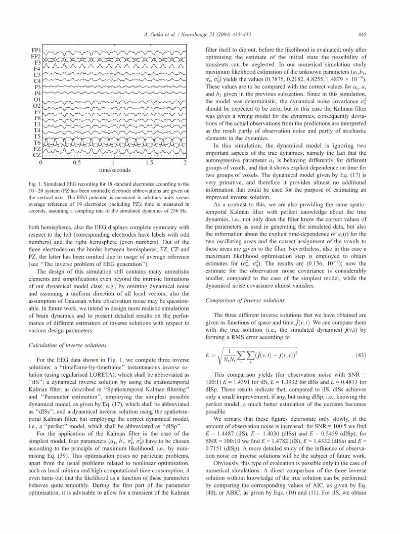
Fig. 1. Simulated EEG recording for 18 standard electrodes according to the
10–20 system (PZ has been omitted); electrode abbreviations are given on
the vertical axis. The EEG potential is measured in arbitrary units versus
average reference of 19 electrodes (including PZ); time is measured in
seconds, assuming a sampling rate of the simulated dynamics of 256 Hz.
A. Galka et al. / NeuroImage 23 (2004) 435–453 445
both hemispheres, also the EEG displays complete symmetry with
respect to the left (corresponding electrodes have labels with odd
numbers) and the right hemisphere (even numbers). Out of the
three electrodes on the border between hemispheres, FZ, CZ and
PZ, the latter has been omitted due to usage of average reference
(see ‘‘The inverse problem of EEG generation’’).
The design of this simulation still contains many unrealistic
elements and simplifications even beyond the intrinsic limitations
of our dynamical model class, e.g., by omitting dynamical noise
and assuming a uniform direction of all local vectors; also the
assumption of Gaussian white observation noise may be question-
able. In future work, we intend to design more realistic simulations
of brain dynamics and to present detailed results on the perfor-
mance of different estimators of inverse solutions with respect to
various design parameters.
Calculation of inverse solutions
For the EEG data shown in Fig. 1, we compute three inverse
solutions: a ‘‘timeframe-by-timeframe’’ instantaneous inverse so-
lution (using regularised LORETA), which shall be abbreviated as
‘‘iIS’’; a dynamical inverse solution by using the spatiotemporal
Kalman filter, as described in ‘‘Spatiotemporal Kalman filtering’’
and ‘‘Parameter estimation’’, employing the simplest possible
dynamical model, as given by Eq. (17), which shall be abbreviated
as ‘‘dISs’’; and a dynamical inverse solution using the spatiotem-
poral Kalman filter, but employing the correct dynamical model,
i.e., a ‘‘perfect’’ model, which shall be abbreviated as ‘‘dISp’’.
For the application of the Kalman filter in the case of the
simplest model, four parameters (a1, b1, re2, rg
2) have to be chosen
according to the principle of maximum likelihood, i.e., by mini-
mising Eq. (39). This optimisation poses no particular problems,
apart from the usual problems related to nonlinear optimisation,
such as local minima and high computational time consumption; it
even turns out that the likelihood as a function of these parameters
behaves quite smoothly. During the first part of the parameter
optimisation, it is advisable to allow for a transient of the Kalman
filter itself to die out, before the likelihood is evaluated; only after
optimising the estimate of the initial state the possibility of
transients can be neglected. In our numerical simulation study
maximum likelihood estimation of the unknown parameters (a1,b1,
re2, rg
2) yields the values (0.7875, 0.2182, 4.8255, 1.4879 � 10�6).
These values are to be compared with the correct values for ac, asand b1 given in the previous subsection. Since in this simulation,
the model was deterministic, the dynamical noise covariance rg2
should be expected to be zero; but in this case the Kalman filter
was given a wrong model for the dynamics, consequently devia-
tions of the actual observations from the predictions are interpreted
as the result partly of observation noise and partly of stochastic
elements in the dynamics.
In this simulation, the dynamical model is ignoring two
important aspects of the true dynamics, namely the fact that the
autoregressive parameter a1 is behaving differently for different
groups of voxels, and that it shows explicit dependence on time for
two groups of voxels. The dynamical model given by Eq. (17) is
very primitive, and therefore it provides almost no additional
information that could be used for the purpose of estimating an
improved inverse solution.
As a contrast to this, we are also providing the same spatio-
temporal Kalman filter with perfect knowledge about the true
dynamics, i.e., not only does the filter know the correct values of
the parameters as used in generating the simulated data, but also
the information about the explicit time-dependence of a1(t) for the
two oscillating areas and the correct assignment of the voxels to
these areas are given to the filter. Nevertheless, also in this case a
maximum likelihood optimisation step is employed to obtain
estimates for (re2, rg
2). The results are (0.156, 10�7); now the
estimate for the observation noise covariance is considerably
smaller, compared to the case of the simplest model, while the
dynamical noise covariance almost vanishes.
Comparison of inverse solutions
The three different inverse solutions that we have obtained are
given as functions of space and time, jðv; tÞ. We can compare them
with the true solution (i.e., the simulated dynamics) j(v,t) by
forming a RMS error according to
E ¼ffiffiffiffiffiffiffiffiffiffiffiffiffiffiffiffiffiffiffiffiffiffiffiffiffiffiffiffiffiffiffiffiffiffiffiffiffiffiffiffiffiffiffiffiffiffiffiffiffiffiffiffiffiffiffiffiffiffiffiffi1
NvNt
Xv
Xt
ð jðv; tÞ � jðv; tÞÞ2s
ð43Þ
This comparison yields (for observation noise with SNR =
100:1) E = 1.4391 for iIS, E = 1.3932 for dISs and E = 0.4813 for
dISp. These results indicate that, compared to iIS, dISs achieves
only a small improvement, if any, but using dISp, i.e., knowing the
perfect model, a much better estimation of the currents becomes
possible.
We remark that these figures deteriorate only slowly, if the
amount of observation noise is increased: for SNR = 100:5 we find
E = 1.4487 (iIS), E = 1.4030 (dISs) and E = 0.5459 (dISp); for
SNR = 100:10 we find E = 1.4782 (iIS), E = 1.4332 (dISs) and E =
0.7151 (dISp). A more detailed study of the influence of observa-
tion noise on inverse solutions will be the subject of future work.
Obviously, this type of evaluation is possible only in the case of
numerical simulations. A direct comparison of the three inverse
solution without knowledge of the true solution can be performed
by comparing the corresponding values of AIC, as given by Eq.
(40), or ABIC, as given by Eqs. (10) and (11). For iIS, we obtain
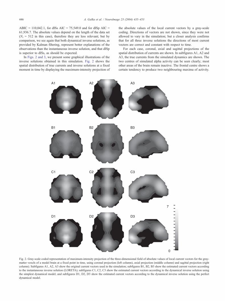
A. Galka et al. / NeuroImage 23 (2004) 435–453446
ABIC = 110,042.1, for dISs AIC = 75,549.0 and for dISp AIC =
61,936.7. The absolute values depend on the length of the data set
(Nt = 512 in this case), therefore they are less relevant; but by
comparison, we see again that both dynamical inverse solutions, as
provided by Kalman filtering, represent better explanations of the
observations than the instantaneous inverse solution, and that dISp
is superior to dISs, as should be expected.
In Figs. 2 and 3, we present some graphical illustrations of the
inverse solutions obtained in this simulation. Fig. 2 shows the
spatial distribution of true currents and inverse solutions at a fixed
moment in time by displaying the maximum-intensity projection of
Fig. 2. Gray-scale coded representation of maximum-intensity projection of the thr
matter voxels of a model brain at a fixed point in time, using coronal projection (
column). Subfigures A1, A2, A3 show the original current vectors used in the simu
to the instantaneous inverse solution (LORETA); subfigures C1, C2, C3 show the
the simplest dynamical model; and subfigures D1, D2, D3 show the estimated cu
dynamical model.
the absolute values of the local current vectors by a gray-scale
coding. Directions of vectors are not shown, since they were not
allowed to vary in the simulation; but a closer analysis confirms
that for all three inverse solutions the directions of most current
vectors are correct and constant with respect to time.
For each case, coronal, axial and sagittal projections of the
spatial distribution of currents are shown. In subfigures A1, A2 and
A3, the true currents from the simulated dynamics are shown. The
two centres of simulated alpha activity can be seen clearly; most
other areas of the brain remain inactive. The frontal centre shows a
certain tendency to produce two neighbouring maxima of activity.
ee-dimensional field of absolute values of local current vectors for the gray-
left column), axial projection (middle column) and sagittal projection (right
lation; subfigures B1, B2, B3 show the estimated current vectors according
estimated current vectors according to the dynamical inverse solution using
rrent vectors according to the dynamical inverse solution using the perfect
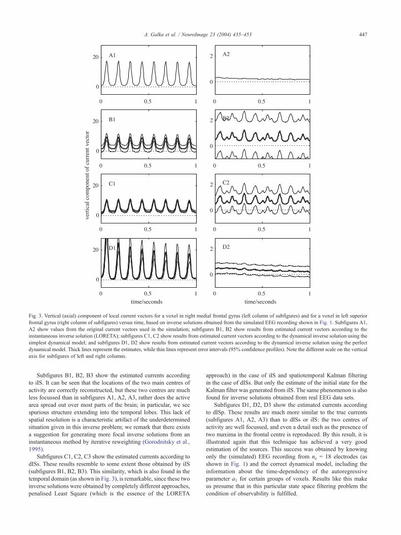
Fig. 3. Vertical (axial) component of local current vectors for a voxel in right medial frontal gyrus (left column of subfigures) and for a voxel in left superior
frontal gyrus (right column of subfigures) versus time, based on inverse solutions obtained from the simulated EEG recording shown in Fig. 1. Subfigures A1,
A2 show values from the original current vectors used in the simulation; subfigures B1, B2 show results from estimated current vectors according to the
instantaneous inverse solution (LORETA); subfigures C1, C2 show results from estimated current vectors according to the dynamical inverse solution using the
simplest dynamical model; and subfigures D1, D2 show results from estimated current vectors according to the dynamical inverse solution using the perfect
dynamical model. Thick lines represent the estimates, while thin lines represent error intervals (95% confidence profiles). Note the different scale on the vertical
axis for subfigures of left and right columns.
A. Galka et al. / NeuroImage 23 (2004) 435–453 447
Subfigures B1, B2, B3 show the estimated currents according
to iIS. It can be seen that the locations of the two main centres of
activity are correctly reconstructed, but these two centres are much
less focussed than in subfigures A1, A2, A3, rather does the active
area spread out over most parts of the brain; in particular, we see
spurious structure extending into the temporal lobes. This lack of
spatial resolution is a characteristic artifact of the underdetermined
situation given in this inverse problem; we remark that there exists
a suggestion for generating more focal inverse solutions from an
instantaneous method by iterative reweighting (Gorodnitsky et al.,
1995).
Subfigures C1, C2, C3 show the estimated currents according to
dISs. These results resemble to some extent those obtained by iIS
(subfigures B1, B2, B3). This similarity, which is also found in the
temporal domain (as shown in Fig. 3), is remarkable, since these two
inverse solutions were obtained by completely different approaches,
penalised Least Square (which is the essence of the LORETA
approach) in the case of iIS and spatiotemporal Kalman filtering
in the case of dISs. But only the estimate of the initial state for the
Kalman filter was generated from iIS. The same phenomenon is also
found for inverse solutions obtained from real EEG data sets.
Subfigures D1, D2, D3 show the estimated currents according
to dISp. These results are much more similar to the true currents
(subfigures A1, A2, A3) than to dISs or iIS: the two centres of
activity are well focussed, and even a detail such as the presence of
two maxima in the frontal centre is reproduced. By this result, it is
illustrated again that this technique has achieved a very good
estimation of the sources. This success was obtained by knowing
only the (simulated) EEG recording from nc = 18 electrodes (as
shown in Fig. 1) and the correct dynamical model, including the
information about the time-dependency of the autoregressive
parameter a1 for certain groups of voxels. Results like this make
us presume that in this particular state space filtering problem the
condition of observability is fulfilled.
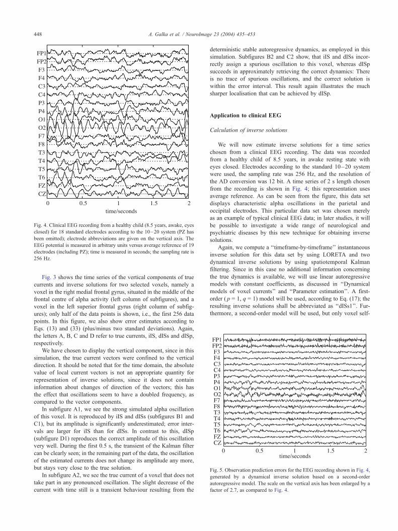
Fig. 4. Clinical EEG recording from a healthy child (8.5 years, awake, eyes
closed) for 18 standard electrodes according to the 10–20 system (PZ has
been omitted); electrode abbreviations are given on the vertical axis. The
EEG potential is measured in arbitrary units versus average reference of 19
electrodes (including PZ); time is measured in seconds; the sampling rate is
256 Hz.
Fig. 5. Observation prediction errors for the EEG recording shown in Fig. 4,
generated by a dynamical inverse solution based on a second-order
autoregressive model. The scale on the vertical axis has been enlarged by a
factor of 2.7, as compared to Fig. 4.
A. Galka et al. / NeuroImage 23 (2004) 435–453448
Fig. 3 shows the time series of the vertical components of true
currents and inverse solutions for two selected voxels, namely a
voxel in the right medial frontal gyrus, situated in the middle of the
frontal centre of alpha activity (left column of subfigures), and a
voxel in the left superior frontal gyrus (right column of subfig-
ures); only half of the data points is shown, i.e., the first 256 data
points. In this figure, we also show error estimates according to
Eqs. (13) and (33) (plus/minus two standard deviations). Again,
the letters A, B, C and D refer to true currents, iIS, dISs and dISp,
respectively.
We have chosen to display the vertical component, since in this
simulation, the true current vectors were confined to the vertical
direction. It should be noted that for the time domain, the absolute
value of local current vectors is not an appropriate quantity for
representation of inverse solutions, since it does not contain
information about changes of direction of the vectors; this has
the effect that oscillations seem to have a doubled frequency, as
compared to the vector components.
In subfigure A1, we see the strong simulated alpha oscillation
of this voxel. It is reproduced by iIS and dISs (subfigures B1 and
C1), but its amplitude is significantly underestimated; error inter-
vals are larger for iIS than for dISs. In contrast to this, dISp
(subfigure D1) reproduces the correct amplitude of this oscillation
very well. During the first 0.5 s, the transient of the Kalman filter
can be clearly seen; in the remaining part of the data, the oscillation
of the estimated currents does not change its amplitude any more,
but stays very close to the true solution.
In subfigure A2, we see the true current of a voxel that does not
take part in any pronounced oscillation. The slight decrease of the
current with time still is a transient behaviour resulting from the
deterministic stable autoregressive dynamics, as employed in this
simulation. Subfigures B2 and C2 show, that iIS and dISs incor-
rectly assign a spurious oscillation to this voxel, whereas dISp
succeeds in approximately retrieving the correct dynamics: There
is no trace of spurious oscillations, and the correct solution is
within the error interval. This result again illustrates the much
sharper localisation that can be achieved by dISp.
Application to clinical EEG
Calculation of inverse solutions
We will now estimate inverse solutions for a time series
chosen from a clinical EEG recording. The data was recorded
from a healthy child of 8.5 years, in awake resting state with
eyes closed. Electrodes according to the standard 10–20 system
were used, the sampling rate was 256 Hz, and the resolution of
the AD conversion was 12 bit. A time series of 2 s length chosen
from the recording is shown in Fig. 4; this representation uses
average reference. As can be seen from the figure, this data set
displays characteristic alpha oscillations in the parietal and
occipital electrodes. This particular data set was chosen merely
as an example of typical clinical EEG data; in later studies, it will
be possible to investigate a wide range of neurological and
psychiatric diseases by this new technique for obtaining inverse
solutions.
Again, we compute a ‘‘timeframe-by-timeframe’’ instantaneous
inverse solution for this data set by using LORETA and two
dynamical inverse solutions by using spatiotemporal Kalman
filtering. Since in this case no additional information concerning
the true dynamics is available, we will use linear autoregressive
models with constant coefficients, as discussed in ‘‘Dynamical
models of voxel currents’’ and ‘‘Parameter estimation’’. A first-
order ( p = 1, q = 1) model will be used, according to Eq. (17); the
resulting inverse solutions shall be abbreviated as ‘‘dISs1’’. Fur-
thermore, a second-order model will be used, but only voxel self-
A. Galka et al. / NeuroImage 23 (2004) 435–453 449
interaction will be second order, while neighbour interaction will
remain first order ( p = 2, q = 1); this model results from adding an
additional term a2I3 jðv; t�2) in Eq. (17). The resulting inverse
solutions shall be abbreviated as ‘‘dISs2’’.
In the case p = 1, q = 1 maximum likelihood estimation of the
unknown parameters (a1, b1, re2, rg
2) yields the values (0.7875,
0.2182, 4.8255, 1.4879 � 10�6), and for p = 2, q = 1 we find (a1,
a2, b1, re2, rg
2) = (0.9923, �0.7101, 0.7993, 3.3412, 1.0507). These
solutions may not yet represent global maxima, but we believe that
they correspond to inverse solutions whose properties are qualita-
tively similar to those of the global solution.
Comparison of inverse solutions
Unlike with the simulation study of ‘‘Application to simulated
EEG’’, we are in this case unable to compare the inverse solutions
directly with the true solution; consequently, they have to be
evaluated and compared by statistical criteria. For the instanta-
neous solution (iIS), we obtain ABIC = 112,328.4, while for the
dynamical inverse solution with p = 1, q = 1 (dISs1) we obtain
Fig. 6. Gray-scale-coded representation of maximum-intensity projection of the thr
matter voxels of a model brain at a fixed point in time, using coronal projection (
column), based on inverse solutions obtained from the EEG recording shown in Fi
the instantaneous inverse solution (LORETA); subfigures C1, C2, C3 show the es
first-order autoregressive model; and subfigures D1, D2, D3 show the estimated c
order autoregressive model.
AIC = 88,990.1 and for p = 2, q = 1 (dISs2) AIC = 87,131.3.
These values confirm again that the dynamical inverse solutions
represent better explanations of the observations than the
instantaneous inverse solution. We also see that increasing the
model order helps to further decrease the AIC, but at the
expense of a more time-consuming parameter estimation, due
to the increased dimensionality of the parameter space.
The results of this state estimation problem can be further
illustrated by showing in Fig. 5 the residuals of the data prediction,
i.e., the whitened time series (compare ‘‘Dynamical models of
voxel currents’’). The figure demonstrates the success of explain-
ing most of the structure in the observations through the dynamical
model; however, it can also be seen that some structure is
remaining, especially some components obviously belonging to
the alpha oscillation. Improved dynamical models will be required
to capture also these components.
In Figs. 6 and 7, we again present graphical illustrations of
spatial and temporal properties of the inverse solutions. Fig. 6
shows the spatial distribution of inverse solutions obtained by iIS
(subfigures B1, B2 and B3), dISs1 (subfigures C1, C2 and C3)
ee-dimensional field of absolute values of local current vectors for the gray-
left column), axial projection (middle column) and sagittal projection (right
g. 4. Subfigures B1, B2, B3 show the estimated current vectors according to
timated current vectors according to the dynamical inverse solution using a
urrent vectors according to the dynamical inverse solution using a second-

Fig. 7. Vertical (axial) component of local current vectors for a voxel in right cuneus (left column of subfigures) and for a voxel in right medial frontal gyrus
(right column of subfigures) versus time, based on inverse solutions obtained from the EEG recording shown in Fig. 4. Subfigures B1, B2 show results from
estimated current vectors according to the instantaneous inverse solution (LORETA); subfigures C1, C2 show results from estimated current vectors according
to the dynamical inverse solution using a first-order autoregressive model; and subfigures D1, D2 show results from the estimated current vectors according to
the dynamical inverse solution using a second-order autoregressive model. Thick lines represent the estimates, while thin lines represent error intervals (95%
confidence profiles).
A. Galka et al. / NeuroImage 23 (2004) 435–453450
and dISs2 (subfigures D1, D2 and D3) at a fixed moment in time,
again by displaying the coronal, axial and sagittal maximum-
intensity projections of the absolute values of the local current
vectors.
From the figure, it can be seen that all three inverse solutions
locate a centre of activity in the occipital region, as should be
expected for EEG data displaying pronounced alpha activity in
parietal and occipital electrodes; in the dynamical inverse solu-
tions, this centre has larger amplitude and appears to be better
localised, compared with neighbouring brain areas. Together with
the superior values of AIC, this result seems to provide evidence
for improved resolution and localisation abilities of the dynamical
inverse solutions.
Fig. 7 shows the time series of the sagittal component of the
inverse solutions for two selected voxels, namely a voxel in the
right cuneus (i.e., in the occipital area; left column of subfigures)
and, as before, a voxel in the right medial frontal gyrus (right
column of subfigures). Error estimates are also shown. The letters
B, C and D refer to iIS, dISs1 and dISs2, respectively. Among
the three projections of the current vectors, for this data set, the
projection onto the sagittal direction showed the largest ampli-
tudes correlated to alpha activity; therefore, we have chosen to
present it.
In subfigures B1, C1, D1, we see for the occipital voxel a
pronounced oscillation representing the alpha activity in the first
half of this data set. All three inverse solutions reconstruct this
oscillation at this voxel, but again we notice that dISs1 and dISs2
find much higher amplitude than iIS. More importantly, the error
intervals of dISs1 and dISs2 are much smaller than those of iIS; in
fact, it turns out that the error estimates for the instantaneous
inverse solutions are so large that any deviation of the vector
component from zero has to be regarded as nonsignificant. Similar
remarks apply to subfigures B2, C2, D2, where dISs1 and dISs2
indicate the presence of a weak low-frequency wave, whereas iIS
fails to find any structure.
It is not the aim of this paper to discuss these results from a
physiological point of view, but primarily to present these new
tools for obtaining improved inverse solutions and to compare
them with a well-known representative of the currently available
algorithms, the LORETA method. In future work, it has to be
investigated in detail, in which respect dynamical inverse solutions
are capable of providing additional relevant information for the
analysis of brain dynamics and for the diagnosis of diseases
affecting the brain. In this paper, our claim of superiority of
dynamical inverse solutions over LORETA inverse solutions is
based on the relative comparison of values of the ABIC and AIC
criteria, regarded as a measure of distance between the estimated
model and the unknown true model.
Conclusion
In this paper, we have addressed the dynamical inverse problem
of EEG generation, being a generalisation of the more traditional
instantaneous problem of EEG generation, and we have presented
a new approach for estimating solutions of this problem from
actual EEG data. This approach is applicable also to MEG data and
to a wide class of other inverse problems arising in the analysis of
biomedical or other data. We have demonstrated how the standard
Kalman filter can be adapted to the case of spatiotemporal
dynamics; an essential precondition for this adaptation was the
concept of spatial whitening, which renders it possible to decom-
pose an intractable high-dimensional filtering problem into a set of
coupled low-dimensional problems that can be solved with mod-
erate computational effort. The application of Kalman filtering has
the additional benefit of providing estimates of the likelihood and
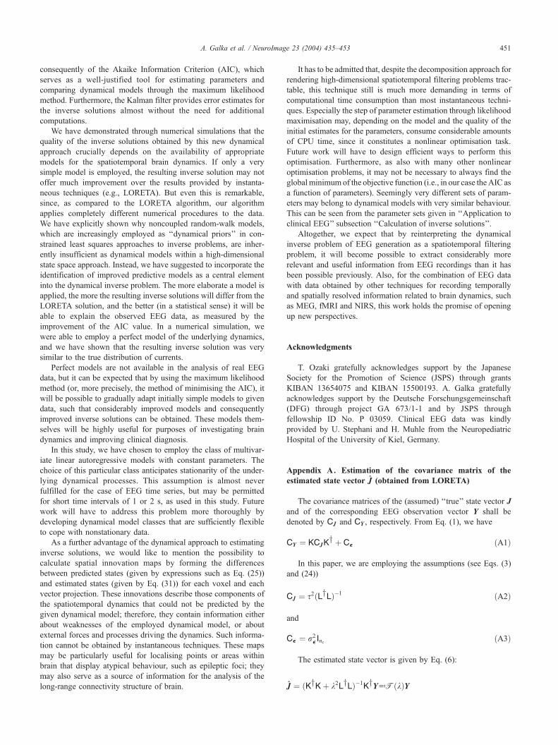
A. Galka et al. / NeuroImage 23 (2004) 435–453 451
consequently of the Akaike Information Criterion (AIC), which
serves as a well-justified tool for estimating parameters and
comparing dynamical models through the maximum likelihood
method. Furthermore, the Kalman filter provides error estimates for
the inverse solutions almost without the need for additional
computations.
We have demonstrated through numerical simulations that the
quality of the inverse solutions obtained by this new dynamical
approach crucially depends on the availability of appropriate
models for the spatiotemporal brain dynamics. If only a very
simple model is employed, the resulting inverse solution may not
offer much improvement over the results provided by instanta-
neous techniques (e.g., LORETA). But even this is remarkable,
since, as compared to the LORETA algorithm, our algorithm
applies completely different numerical procedures to the data.
We have explicitly shown why noncoupled random-walk models,
which are increasingly employed as ‘‘dynamical priors’’ in con-
strained least squares approaches to inverse problems, are inher-
ently insufficient as dynamical models within a high-dimensional
state space approach. Instead, we have suggested to incorporate the
identification of improved predictive models as a central element
into the dynamical inverse problem. The more elaborate a model is
applied, the more the resulting inverse solutions will differ from the
LORETA solution, and the better (in a statistical sense) it will be
able to explain the observed EEG data, as measured by the
improvement of the AIC value. In a numerical simulation, we
were able to employ a perfect model of the underlying dynamics,
and we have shown that the resulting inverse solution was very
similar to the true distribution of currents.
Perfect models are not available in the analysis of real EEG
data, but it can be expected that by using the maximum likelihood
method (or, more precisely, the method of minimising the AIC), it
will be possible to gradually adapt initially simple models to given
data, such that considerably improved models and consequently
improved inverse solutions can be obtained. These models them-
selves will be highly useful for purposes of investigating brain
dynamics and improving clinical diagnosis.
In this study, we have chosen to employ the class of multivar-
iate linear autoregressive models with constant parameters. The
choice of this particular class anticipates stationarity of the under-
lying dynamical processes. This assumption is almost never
fulfilled for the case of EEG time series, but may be permitted
for short time intervals of 1 or 2 s, as used in this study. Future
work will have to address this problem more thoroughly by
developing dynamical model classes that are sufficiently flexible
to cope with nonstationary data.
As a further advantage of the dynamical approach to estimating
inverse solutions, we would like to mention the possibility to
calculate spatial innovation maps by forming the differences
between predicted states (given by expressions such as Eq. (25))
and estimated states (given by Eq. (31)) for each voxel and each
vector projection. These innovations describe those components of
the spatiotemporal dynamics that could not be predicted by the
given dynamical model; therefore, they contain information either
about weaknesses of the employed dynamical model, or about
external forces and processes driving the dynamics. Such informa-
tion cannot be obtained by instantaneous techniques. These maps
may be particularly useful for localising points or areas within
brain that display atypical behaviour, such as epileptic foci; they
may also serve as a source of information for the analysis of the
long-range connectivity structure of brain.
It has to be admitted that, despite the decomposition approach for
rendering high-dimensional spatiotemporal filtering problems trac-
table, this technique still is much more demanding in terms of
computational time consumption than most instantaneous techni-
ques. Especially the step of parameter estimation through likelihood
maximisation may, depending on the model and the quality of the
initial estimates for the parameters, consume considerable amounts
of CPU time, since it constitutes a nonlinear optimisation task.
Future work will have to design efficient ways to perform this
optimisation. Furthermore, as also with many other nonlinear
optimisation problems, it may not be necessary to always find the
global minimumof the objective function (i.e., in our case theAIC as
a function of parameters). Seemingly very different sets of param-
eters may belong to dynamical models with very similar behaviour.
This can be seen from the parameter sets given in ‘‘Application to
clinical EEG’’ subsection ‘‘Calculation of inverse solutions’’.
Altogether, we expect that by reinterpreting the dynamical
inverse problem of EEG generation as a spatiotemporal filtering
problem, it will become possible to extract considerably more
relevant and useful information from EEG recordings than it has
been possible previously. Also, for the combination of EEG data
with data obtained by other techniques for recording temporally
and spatially resolved information related to brain dynamics, such
as MEG, fMRI and NIRS, this work holds the promise of opening
up new perspectives.
Acknowledgments
T. Ozaki gratefully acknowledges support by the Japanese
Society for the Promotion of Science (JSPS) through grants
KIBAN 13654075 and KIBAN 15500193. A. Galka gratefully
acknowledges support by the Deutsche Forschungsgemeinschaft
(DFG) through project GA 673/1-1 and by JSPS through
fellowship ID No. P 03059. Clinical EEG data was kindly
provided by U. Stephani and H. Muhle from the Neuropediatric
Hospital of the University of Kiel, Germany.
Appendix A. Estimation of the covariance matrix of the
estimated state vector J (obtained from LORETA)
The covariance matrices of the (assumed) ‘‘true’’ state vector J
and of the corresponding EEG observation vector Y shall be
denoted by CJ and CY , respectively. From Eq. (1), we have
CY ¼ KCJKy þ C: ðA1Þ
In this paper, we are employing the assumptions (see Eqs. (3)
and (24))
CJ ¼ s2ðLyLÞ�1 ðA2Þ
and
C: ¼ r2: Inc ðA3Þ
The estimated state vector is given by Eq. (6):
J ¼ ðKyK þ k2LyLÞ�1KyYzTðkÞY

A. Galka et al. / NeuroImage 23 (2004) 435–453452
Then, the covariance matrix of the estimated state vector J is
given as
CðiISÞJ
¼ TðkÞCYTyðkÞ ðA4Þ
The product KCJKy in Eq. (A1) yields, using Eqs. (A2) and (8)
s2KðLyLÞ�1K ¼ s2ðKL�1ÞðKL�1Þy ¼ s2US2Uy
Using s = r/k and Eq. (A3), Eq. (A1) becomes
CY ¼ s2ðUS2Uy þ k2Inc Þ ðA5Þ
By inserting Eq. (9) for TðkÞ and Eq. (A5) for CY, we finally
can evaluate Eq. (A4); by rearranging terms, we obtain (using
orthogonality of U)
CðiISÞJ
¼ s2L�1Vð1Þdiags2i
s2i þ k2
!Vð1ÞyðLyÞ�1
which is the desired result.
The diagonal elements of CðiISÞJ
provide variances for each
element of the state vector J; since in our implementation, the
estimates for s and k result from an optimisation step applied to the
complete time series, these variances themselves will not depend
on time, unlike the state estimates J ¼ JðtÞ; if, however, variancesof the modulus j(v, t) of local vectors j(v,t) are computed, these will
become time-dependent through Gaussian error propagation:
r2j ðv; tÞ ¼
1
j2ðv; tÞ
� ðjxðv; tÞrjxðvÞÞ2 þ ðjyðv; tÞrjy ðvÞÞ
2 þ ðjzðv; tÞrjzðvÞÞ2
� �ðA6Þ
Alternatively, explicitly time-dependent local variances could be
obtained by repeating the optimisation on a moving window, but in
this paper we have not used this option.
References
Akaike, H., 1974. A new look at the statistical model identification. IEEE
Trans. Autom. Control 19, 716–723.
Akaike, H., 1980a. Seasonal adjustment by a Bayesian modeling. J. Time
Ser. Anal. 1, 1–13.
Akaike, H., 1980b. Likelihood and the Bayes procedure. In: Bernardo,
M.H., De Groot, M.H., Lindley, D.U., Smith, A.F.M. (Eds.), Bayesian
Statistics. University Press, Valencia, Spain, pp. 141–166.
Akaike, H., 1985. Prediction and entropy. In: Atkinson, A.C., Fienberg,
S.E. (Eds.), A Celebration of Statistics. Springer, Berlin, pp. 1–24.
Ary, J.P., Klein, S.A., Fender, D.H., 1981. Location of sources of evoked
scalp potentials: corrections for skull and scalp thickness. IEEE Trans.
Biomed. Eng. 28, 447–452.
Baillet, S., Garnero, L., 1997. A Bayesian approach to introducing ana-
tomo-functional priors in the EEG/MEG inverse problem. IEEE Trans.
Biomed. Eng. 44, 374–385.
Baillet, S., Mosher, J.C., Leahy, R.M., 2001. Electromagnetic brain map-
ping. IEEE Signal Process. Mag., 14–30 (November).
Baroudi, D., Kaipio, J., Somersalo, E., 1998. Dynamical electric wire to-
mography: a time series approach. Inverse Probl. 14, 799–813.
Bosch-Bayard, J., Valdes-Sosa, P.A., Virues-Alba, T., Aubert-Vazquez, E.,
Roy John, E., Harmony, T., Riera-Dıaz, J.J., Trujillo-Barreto, N., 2001.
3D statistical parametric mapping of EEG source spectra by means of
variable resolution electromagnetic tomography (VARETA). Clin. Elec-
troencephalogr. 32, 47–61.
Buchner, H., Knoll, G., Fuchs, M., Rienacker, A., Beckmann, R., Wagner,
J., Silny, J., Pesch, J., 1997. Inverse localization of electric dipole
current sources in finite element models of the human head. Electro-
encephalogr. Clin. Neurophysiol. 102, 267–278.
Chui, C.K., Chen, G., 1999. , third ed.Kalman filtering: with real-time
applications. Springer Series in Information Sciences, vol. 17. Springer,
Berlin.
Darvas, F., Schmitt, U., Louis, A.K., Fuchs, M., Knoll, G., Buchner, H.,
2001. Spatiotemporal current density reconstruction (stCDR) from
EEG/MEG data. Brain Topogr. 13, 195–207.
Gorodnitsky, I.F., Georg, J.S., Rao, B.D., 1995. Neuromagnetic source
imaging with FOCUSS: a recursive weighted minimum norm algo-
rithm. Electroencephalogr. Clin. Neurophysiol. 95, 231–251.
Grave de Peralta Menendez, R., Gonzalez Andino, S., 1999. A critical
analysis of linear inverse solutions to the neuroelectromagnetic inverse
problem. IEEE Trans. Biomed. Eng. 45, 440–448.
Greenblatt, R., 1993. Probabilistic reconstruction of multiple sources in the
bioelectromagnetic inverse problem. Inverse Probl. 9, 271–284.
Hamalainen, M.S., Ilmoniemi, R.J., 1984. Interpreting measured mag-
netic fields of the brain: estimates of current distributions. Technical
Report TKK-F-A559. Helsinki University of Technology, Espoo
(Finland).
Hjorth, B., 1980. Source derivation simplifies topographical EEG interpre-
tation. Am. J. EEG Technol. 20, 121–132.
Hofmann, B., 1986. Regularization for Applied Inverse and Ill-Posed Prob-
lems Teubner, Leipzig.
Jiang, X.-Q., 1992. Bayesian Methods for Modeling, Identification
and Estimation of Stochastic Systems. PhD thesis, Department
of Statistical Science, Graduate University for Advanced Studies,
Tokyo.
Jirsa, V.K., Jantzen, K.J., Fuchs, A., Kelso, J.A.S., 2002. Spatiotemporal
forward solution of the MEG using network modeling. IEEE Trans.
Med. Imag. 21, 493–504.
Kailath, Th., 1980. Linear Systems. Information and System Sciences
Series. Prentice-Hall, Englewood Cliffs.
Kaipio, J.P., Karjalainen, P.A., Somersalo, E., Vauhkonen, M., 1999. State
estimation in time-varying electrical impedance tomography. Ann. N. Y.
Acad. Sci. 873, 430–439.
Kalman, R.E., Falb, P.L., Arbib, M.A., 1969. Topics in Mathematical Sys-
tem Theory. International Series in Pure and Applied Mathematics
McGraw-Hill, New York.
Karjalainen, P.A., 1997. Regularization and Bayesian Methods for Evoked
Potential Estimation. Kuopio University Publications C. Natural and
Environmental Sciences, Kuopio, vol. 61.
Lawson, C.L., Hanson, R.J., 1974. Solving Least Squares Problems Pren-
tice-Hall, Englewood Cliffs.
Mazziotta, J.C., Toga, A., Evans, A.C., Fox, P., Lancaster, J., 1995. A
probabilistic atlas of the human brain: theory and rationale for its de-
velopment. NeuroImage 2, 89–101.
Mosher, J.C., Lewis, P., Leahy, R., 1992. Multiple dipole modeling and
localization from spatio-temporal MEG data. IEEE Trans. Biomed. Eng.
39, 541–557.
Nunez, P.L., 1981. Electrical Fields of the Brain Oxford Univ. Press, New
York.
Ozaki, T., Jimenez, J.C., Haggan-Ozaki, V., 2000. The role of the likeli-
hood function in the estimation of chaos models. J. Time Ser. Anal. 21,
363–387.
Pascual-Marqui, R.D., 1999. Review of methods for solving the EEG
inverse problem. Int. J. Bioelectromagn. 1, 75–86.
Pascual-Marqui, R.D., 2002. Standardized low resolution brain electromag-
netic tomography (sLORETA): technical details. Methods Find. Exp.
Clin. Pharmacol. 24D, 5–12.
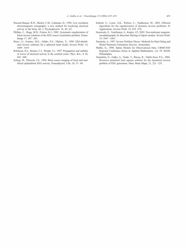
A. Galka et al. / NeuroImage 23 (2004) 435–453 453
Pascual-Marqui, R.D., Michel, C.M., Lehmann, D., 1994. Low resolution
electromagnetic tomography: a new method for localizing electrical
activity in the brain. Int. J. Psychophysiol. 18, 49–65.
Phillips, C., Rugg, M.D., Friston, K.J., 2002. Systematic regularization of
linear inverse solutions of the EEG source localization problem. Neuro-
Image 17, 287–301.
Riera, J.J., Fuentes, M.E., Valdes, P.A., Oharriz, Y., 1998. EEG-distrib-
uted inverse solutions for a spherical head model. Inverse Probl. 14,
1009–1019.
Robinson, P.A., Rennie, C.J., Wright, J.J., 1997. Propagation and stability
of waves of electrical activity in the cerebral cortex. Phys. Rev., E 56,
826–840.
Scherg, M., Ebersole, J.S., 1994. Brain source imaging of focal and mul-
tifocal epileptiform EEG activity. Neurophysiol. Clin. 24, 51–60.
Schmitt, U., Louis, A.K., Wolters, C., Vauhkonen, M., 2002. Efficient
algorithms for the regularization of dynamic inverse problems: II.
Applications. Inverse Probl. 18, 659–676.
Somersalo, E., Voutilainen, A., Kaipio, J.P., 2003. Non-stationary magneto-
encephalography by Bayesian filtering of dipole models. Inverse Probl.
19, 1047–1063.
Tarantola, A., 1987. Inverse Problem Theory: Methods for Data Fitting and
Model Parameter Estimation Elsevier, Amsterdam.
Wahba, G., 1990. Spline Models for Observational Data. CBMS-NSF
Regional Conference Series in Applied Mathematics, vol. 59. SIAM,
Philadelphia.
Yamashita, O., Galka, A., Ozaki, T., Biscay, R., Valdes-Sosa, P.A., 2004.
Recursive penalized least squares solution for the dynamical inverse
problem of EEG generation. Hum. Brain Mapp. 21, 221–235.