A soil data base for the 1:1 million scale windows ... · PDF fileDeliverable D5 A soil data...
32
Project acronym e-SOTER Project full title Regional pilot platform as EU contribution to a Global Soil Observing System Project No 211578 Deliverable D5 A soil data base for the 1:1 million scale windows January 2011 SEVENTH FRAMEWORK PROGRAMME Environment ENV.2007.4.1.3.3 Development of a Global Soil Observing System
Transcript of A soil data base for the 1:1 million scale windows ... · PDF fileDeliverable D5 A soil data...

Project acronym
e-SOTER
Project full title Regional pilot platform as EU contribution to a Global Soil Observing System
Project No 211578
Deliverable D5
A soil data base for the 1:1 million scale windows
January 2011
SEVENTH FRAMEWORK PROGRAMME Environment
ENV.2007.4.1.3.3 Development of a Global Soil Observing System

Report Deliverable No D5 e‐SOTER
Document Information
Deliverable number D5 Deliverable title A soil data base for the 1:1 million scale windows Period covered n.a. Due date of deliverable 31/08/2010 Actual date of deliverable 10/01/2011 Author(s) Erika Michéli, Vince Láng, Márta Fuchs, István Waltner,
Tamás Szegi (SIU), Endre Dobos, Anna Seres, Péter Vadnai (Unimis), Vincent van Engelen, Koos Dijkshoorn (ISRIC), Joel Daroussin (INRA), Einar Eberhardt, Uhlrich Schuler (BGR), Tereza Zadorova, Josef Kozak (CULS), Jacqueline Hannam, Steve Hallett (CU), Ganlin Zhang, Zhao Yuguo (ISSCAS), Riad Balaghi, Rachid Moussadek (INRA Maroc)
Participants All WP1 and WP2 partners Work package 2 Work package title Development of a methodology to integrate soil data from
legacy and RS sources Dissemination level PU Version 1.0
History of Versions
Version Date Status Author Approval level 1.0 10/01/2011 Version 1 Erika Michéli
2

Report Deliverable No D5 e‐SOTER
Table of Contents
Table of Contents .................................................................................................................................... 3
1. Summary of Deliverable D5................................................................................................................. 4
1.1 General statements .................................................................................................................... 4
2. Task 2.1 Generating spatial soil information for the 1:1 M windows ................................................. 4
2.1 The traditional SOTER approach ................................................................................................ 4
2.2 The e‐SOTER approach................................................................................................................ 5
2.3 The definition of the significant WRB properties, diagnostics and horizons.............................. 6
2.4 The collection of legacy data and the development of training datasets ................................ 10
2.5 The development of layers of DPDH using image classification procedures........................... 11
2.6 The definition of the classification rules to define the existing soil classes ............................. 15
2.7 The allocation of the soil components in the SOTER database ................................................ 18
2.8 The allocation of the soil info to the SOTER database, the definition of the soil components............................................................................................................Error! Bookmark not defined.
3. Task 2.2 Compilation of a harmonized soil data base for the 1:1 million‐scale windows ................ 20
3. 1 The revised e‐SOTER data structure ........................................................................................ 20
3.3 Development of translation algorithms correlation tools for the harmonization process ...... 21
3. 4. Definition of representative profiles for soil components of the e‐SOTER units ................... 23
References............................................................................................................................................. 23
ANNEX I: MODIS satellite images data sheet ........................................................................................ 25
ANNEX II. The simplified criteria for the expected WRB diagnostics ................................................... 28
ANNEX III. The simplified set of criteria for the expected WRB qualifiers ........................................... 31
3

Report Deliverable No D5 e‐SOTER
1. Summary of Deliverable D5
This deliverable of the e‐SOTER project includes the coverage of the SOTER soil units for the four 1:1
million scale windows with harmonized soil classification and analytical soil data in a revised SOTER
soil component data structure.
The deliverable has the following parts:
1. Procedure of the development of the e‐SOTER soil units;
2. The development of the revised data structure;
3. Procedure of the development of the harmonized data base;
4. Development of translation algorithms and correlation tools.
1.1 General statements
Work package one delivered the 1:1 million scale SOTER geometric databases of the terrain units for
the windows in Europe, Morocco and S‐China. WP2 delivers the spatial and semantic soil information
for the windows.
The first task T2.1. was to generate spatial soil information for the four 1:1 million‐scale windows.
The second T2.2. task was the compilation of a harmonized soil data base for the 1:1 million‐scale
windows. T2.2.1 subtask was to revise the soil component data structure and coding, T.2.2.2 subtask
was to develop the attribute data base translated into the new standards and T2.2.3. was to develop
translation algorithms and correlation tools for the harmonization process. The deliverable itself if
the coverage of the SOTER soil units for the four 1:1 million‐scale windows with harmonized soil
classification and analytical soil data in a revised SOTER soil component data structure.
2. Task 2.1 Generating spatial soil information for the 1:1 M windows
2.1 The traditional SOTER approach
Soil information in SOTER is presented as associations of soil types with their estimated share within
the polygons. At this level only the soil types are named (called soil component) and some basic
characteristics, like texture, surface rockiness and stoniness and the estimated type, extent and level
of erosion are given. Other soil properties are given only for representative soil profiles linked to
each of the soil components. These profiles have an extensive list of chemical and physical properties
4

Report Deliverable No D5 e‐SOTER
for each genetic horizon to help the user estimating the properties for the whole polygon. Therefore,
the use of SOTER requires the understanding of soil properties. This characteristic of the data limits
the use of the database, but at the same time limits the misuse of the database as well.
Summary of the representation of the soil info within the traditional SOTER approach
‐ The spatial delineations, the so‐called SOTER units, do not represent single soil types. The
delineation aims to define homogeneous soil forming units with typical soil type and associations
of soil types rather than the real extent of soil units. This approach is typical for small scale
databases.
‐ Soil Information is presented on the Soil Component level as pure/consociation or
associations/complexes of soil types.
‐ The associations for each polygon are defined after correlating/translating the national
classification units into the FAO or WRB system. The associations and complexes are
characterized with their percentage of coverage within the SOTER polygon and only very general
properties are given at this level. The percentages are estimated using expert judgment.
‐ Detailed numerical data is provided via the linkage of representative soil profile data to each soil
component.
The traditional approach is used when reliable legacy data exist for the mapped area and the data
can be translated into FAO/WRB diagnostics and units.
Many national classification systems exist with no common thresholds for separating the
classification units. Direct translation/correlation is possible only when the FAO/WRB class
thresholds concur with the thresholds of the national units. In any other case direct translation from
the soil polygons needs expert knowledge or complementary data to correctly classify the input data.
As a result of the correlation, each input polygon of the legacy dataset is reclassified into its
corresponding FAO or WRB unit using all of the linked pre‐ and suffixes, producing a huge number of
potential units. These original units might be combined into more general “mapping” units by the
expert who is uploading the soil info into the SOTER database.
However, there are numerous situations, when the data is not available or accessible for SOTER
database development. This has been one of the major limiting factors for the completion of the
global coverage. Areas with limited data require different approaches. The traditional SOTER uses
FAO or WRB soil units as the major input for the completing the database. The direct estimation of
these units is difficult due to the huge number of potential classes.
2.2 The e‐SOTER approach
The e‐SOTER approach for compiling spatial soil information has been developed to assist the
completion of the SOTER database via developing soil data for areas where there is no full coverage
of legacy data to be harmonized and loaded into the SOTER data structure. The e‐SOTER approach is
5

Report Deliverable No D5 e‐SOTER
based on the defined (from legacy data) master building units of the WRB classification system such
as the diagnostic properties or horizons (DPDH). The approach attempts to estimate the spatial
occurrence probability for the mapped area using remote sensing, digital terrain data and
preprocessed legacy data as training dataset. The success and detail of the approach depend largely
on the quantity and quality of the input training set. In general, some of the related/similar classes
have to be combined and new, more general classes are created to characterize the soil resources of
the polygons. As the WRB includes numerous diagnostics, a limited set of significant units is defined
by an expert group based on the existence and significance of horizons, properties and materials.
Training datasets for this group of diagnostics are derived from legacy data, mainly using profile data
or representative large scale database windows. Each training datasets consists of points or areas
with known existence or absence of the property in question. Using these training datasets for
classifying a complex MODIS/SRTM based image results in numerous continuous layers for each
property having the probabilities of the existence of the diagnostic property. The major advantage of
this approach is that it provides the needed thematic information on important or master soil
properties, like texture, organic matter, salt content etc. At the end, a WRB‐based simplified
classification scheme is developed to identify the WRB soil types for each pixel. This raster database
is used at the end to calculate the percentage of coverage of each soil type within each polygon, the
so called definition of soil components. This approach is suggested to be used, when no contiguous
coverage of legacy data is available for the area. The traditional approach should have a priority over
the e‐SOTER approach, except when the data quality of questionable or non‐satisfactory.
The work flow of the data development has the following major steps:
1) Definition of the significant WRB properties, diagnostics and horizons (DPDH) needed to
characterize the major soil properties and features of the mapped area
2) The collection of legacy data (soil profiles or large scale soil maps) and the development of the
training datasets.
3) The development of the layers of the WRB properties, diagnostics and horizons using image
classification procedures
4) The definition of the classification rules to define the existing soil classes
5) The allocation of the soil info to the SOTER database
2.3 The definition of the significant WRB properties, diagnostics and horizons
The first step is the pre‐stratification of the mapped area. The SOTER approach is based on the
assumption that the landform and the parent material are the most important factors of the soil
formation when working within a relatively small land surface area, like a SOTER polygons, in which
the natural macroclimatic variability is negligible. Therefore the major portion of the climatic
variability is due to the terrain. The vegetation developes in the function of terrain and climate, so
the majority of the vegetation variability is already explained by them. The e‐SOTER approach takes
6

Report Deliverable No D5 e‐SOTER
this assumption as well as a basis for the prestratification of the area. Five classes have been
distinguished: water, mountain, hill, and two plain classes. The fine plain area is the one being plain
and having clay or loam texture (Figure 1.). The coarse plain is the sandy and gravelly textured plain
area. These classes were used to stratify the MODIS/SRTM image to lower the natural variability
within the classes of the soil properties for the classification. The terrain/parent material based pre‐
stratification of the European window are given in Figure 2.and 3.
Figure 1. The stratification rules to define the five terrain/parent material classes
7

Report Deliverable No D5 e‐SOTER
Figure 2. The terrain/parent material based pre‐stratification of the Central European window
The typical soil types for the five terrain/parent material classes and their corresponding diagnostic
horizons and properties were defined by expert knowledge and listed as required information layers
for the soil characterization. This list of the selected DPDHs were than compared with the local legacy
database to test for missing DPDH or real existence/significance of the selected DPDHs in the
database. New DPDH was added to the list when the legacy data proved its importance, or DPDH was
removed when the legacy data did not contain information on the feature, or the frequency of
occurrence was too low to support the classification algorithm. In some cases the DPDH was kept,
even if the data was not supporting its importance, but the experts flagged it as important factor for
the classification.
8

Report Deliverable No D5 e‐SOTER
Figure 3. The terrain/parent material based pre‐stratification of the French‐UK window
9

Report Deliverable No D5 e‐SOTER
2.4 The collection of legacy data and the development of training datasets
The information on texture and on presence of diagnostic organic material were derived from the
texture layers developed in the frame of WP1, like the bare rock surfaces and the consolidated‐
unconsolidated material images as well. These were used as direct input for the classification
algorithm later. The rest of the DPDHs were defined from a representative data set provided by the
partners. The representative datasets could be points or polygons having unique identifier for each
of object. An Excel sheet was created with the identifier column and one column for each selected
DPDH. Experts derived the existing DPDH‐s for each object based on the provided classification units
and the measured properties of the legacy data. A value of 1 was assigned to each object, when the
DPDH in question was existing, a “0” value for the non existing ones, and the cell was left empty
when no decision could be made. Therefore, two classes were created for each DPDH, the existing
class and the non‐existing one; the empty ones were neglected for the classification of the specific
DPDH.
Additional data points were needed when the resulting number of points for the DPDH was
insufficient. By definition, the number of training pixels for each classes has to be at least one more
than the number of image layers used for the classification. In our case, the image had 46 layers, so
the minimum number of training pixels had to be at least 47. In case of less than 47 training pixels for
the classes, the legacy data points were extended “artificially” to a larger region using statistical
thresholds of Euclidian distance for the surrounding pixel values to make sure that similar pixels are
Figure 5. The distribution of the profile dataset for the Central European window
10

Report Deliverable No D5 e‐SOTER
involved into the training procedure. A more similar procedure was to transform the point dataset
into a raster with a size of 1km2, and the whole area of the pixel was used as training area. This latter
approach is simpler, however unavoidably introducing unsupervised uncertainty into the procedure.
Therefore, it was used only when large numbers of points were involved. For the Central European
window 1091 profiles for were available. The distribution of the profiles is shown in Figure 5.
2.5 The development of layers of DPDH using image classification procedures
The DPDH layers were created via an image classification procedure. The background image was
based on MODIS and SRTM derived layers and was set up as follows:
• RS images
MODIS‐multi‐temporal 8 days composites, 11 bands, visible to the thermal spectra, 5
dates covering the none‐snow‐covered period, evenly distributed over the vegetation
period.
MOD09A1: Band 1‐7 (Layers 1‐7), 500 m resolution
MOD11A2: Band 31‐32 (Layers 9‐10), LST (Land Surface Temperature) Day
(Layer 1) and LST Night (Layer 5), 500 meter resolution
See ANNEX I for the derived parameters and band processing steps
• Digital terrain model, SRTM
See ANNEX II for the derived parameters and band processing steps
In order to strengthen the performance of the classification, multi‐temporal images of none‐altered
MODIS bands were compiled into a 55 layers image representing the visible, NIR, MIR and thermal
bands, and also to capture the temporal environmental conditions and changes that reveal to surface
conditions and therefore to the soil/parent material properties, like speed of wetting and drying out,
cooling down or warming up, which are parameters strongly correlating with the texture, colour,
water content and water holding capacity. However, the 55 layers have a significant portion of
information overlapping, redundant info in the images, hence a PCA was used to decrease the
number of input images and de‐correlate the bands information. The best 15 PCA component was
maintained and incorporated into the final image.
There were many attempts recorded in the literature to use band ratios to identify certain lithology
classes or to highlight/enhance lithology differences in Landsat images. These band ratios were
adopted to MODIS and were derived for each of the 5 dates, resulting in 15 other images, that have
been added to the final image.
Previous studies also suggested to use surface temperature information, like the thermal bands of
the MODIS (Bands 31, 32) and the LST (Land Surface Temperature) products (night and day) that
have been derived from them. The daily temperate fluctuation is a function of the thermal capacity
11

Report Deliverable No D5 e‐SOTER
of the surface material, which is the function of the kind of material, texture, color and water
content, basically the factors we are interested in. Therefore, a new normalized band combination
was developed. The daily temperature difference were calculated with simply subtracting the LST
night from the LST day, and the values were multiplied with the ratio of the LST(max for the whole
area)/LST(day) to reduce the effect of the climatic variation due to the difference in potential energy
intake from the sun. These were calculated for each date as well.
SRTM data was used in combination with the MODIS derived layers as well. Annex II of the WP1
report gives the details for the derived parameters. The basic parameters are:
• Elevation (sinks are filled up to certain level)
• Slope percent
• Relief Intensity
• Potential Drainage Density
• Groundwater level
• Topographic Wetness Index
• Upland/Lowland
Convexity (not added to the basic image, used only for the colluvial image derivation)
The listed derivates are either used in the SOTER methodology already, or believed to add significant
information for differentiating between the classified parameters. The SRTM images were degraded
to the level of MODIS resolution and a 43 layers image containing the 15 PCA layers, 8 SRTM
derivatives, 5 normalized LST difference images and 15 band ratios.
Besides of the 43 layers described above, three additional layers were added to the image to
represent the climatic variability. These were the images of Easting and Northing, which defines the
geographic location, and the distance from the see. With these extra three layers a 46 layers image
was developed and used for the classification.
Probability classification for each DPDH showing the likelihood of occurrence of a certain diagnostic for the supporting pixel area, continuous layers of occurrence likelihood for each pixels
As a result of the DPDH selection procedure the following DPDH layers were created:
1. Spodic Horizon Class Probability 2. Argic Horizon Class Probability 3. Cambic Horizon Class Probability 4. Vertisol Class Probability (only Vertisol vertic horizons) 5. Salic Horizon Class Probability 6. Natric Horizon Class Probability 7. Gleyic‐stagnic‐Reducing cond. Class Probability 8. Mollic Horizon Class Probability 9. Calcic Horizon Class Probability 10. Calcisol Class Probability (only Calcisol calcic horizons)
12

Report Deliverable No D5 e‐SOTER
11. Dystric Class Probability 12. Eutric Class Probability
The first step was to create a point coverage from the profile database for each DPDH using only the points having a value of 1 or 0, meaning that the DPDH in question does or does not exist on the certain location. These points were used as training dataset for the two classes in the supervised classification. The number of profiles for each DPDH of the Central European window are listed in Table 1. Signature files for each DPDH were created from the training dataset and used for Class probability classification. The classification was performed using the ClassProb command of the ArcGIS software setting the range of values between 0 and 100, where the value of 50 means equal possibility of the 2 classes (existing or missing DPDH), the higher values mean higher possibility for the existence, while the lower for the missing DPDH. The mapped area was pre‐stratified into the terrain/PM classes described above and the classification of the DPDHs were done simultaneously and individually for the five areas. At the end the 5 classified images of the same DPDH were mosaiced together to create the final probability image for each DPDH. Example of the probability layers are shown in Figure 6.
Twelve probability layers were created for the Central European window this way, which were later combined into a layer stack in a predefined order. This layerstack is loaded into the WRB reference soil group (WRB RSG) classification module, so the order of the layers had to be standardized.
The list of WRB properties, diagnostics and horizons (DPDH) and the image source in the layerstack for the CE window is given in Table 2.
Table 1. The number of training points for the classified DPDHs
No Yes Spodic 1072 12Argic 526 545Cambic 728 345Vertisol 951 140Salic 1049 16Natric 1071 20Gleyic Stagnic strec 815 208Mollic 712 355Calcic 821 224Calcisol 1079 12Dystric 322 528Eutric 528 322
Table 2. The list of WRB properties, diagnostics and horizons (DPDH) and the image source in the layerstack for the CE:
1. Terrain type with 5 classes (reclassified from the SOTER polygons developed in WP1) : 1. fine plain 2. coarse plain 3. hill
13

Report Deliverable No D5 e‐SOTER
4. mountain 5. water
2. Consolidated‐unconsolidated image developed in WP1:
1. consolidated 2. unconsolidated
3. Texture image developed in WP1
4. Bare rock image developed in WP1 5. Spodic Horizon Class Probability 6. Argic Horizon Class Probability 7. Cambic Horizon Class Probability 8. Vertisol Class Probability (only Vertisol vertic horizons) 9. Salic Horizon Class Probability 10. Natric Horizon Class Probability 11. Gleyic‐stagnic‐Reducing cond. Class Probability 12. Mollic Horizon Class Probability 13. Calcic Horizon Class Probability 14. Calcisol Class Probability (only Calcisol calcic horizons) 15. Dystric Class Probability 16. Eutric Class Probability
14

Report Deliverable No D5 e‐SOTER
Figure 6. Examples of the probability layers
2.6 The definition of the classification rules to define the existing soil classes The last step of the procedure was the classification of the WRB reference soil groups (RSG). In order to do so a simplified WRB classification tree was developed to estimate the most likely RSG for each pixel (Table 3). A nested conditional function was developed to classify/define the corresponding RSG for each pixels using the layerstack as input. This classification tree depends strongly on detail and content of the legacy data. The one shown below was applied to the Central European window soil types and to the available set of soil information. The more complete soil data, the more detailed classification tree and the more refined RSG classes can be elaborated. The majority of the real applications require the combination of certain classes into groups of similar or related soil types.
An ArcGIS module containing the nested conditional function system was developed and made available for the public to avoid the potential mistakes in the procedure. The output of the module is a classified RSG image, shown in Figure 7.
15

Report Deliverable No D5 e‐SOTER
Figure 7. The WRB Reference soil groups of the Central European window
16

Report Deliverable No D5 e‐SOTER
Table 3. Simplified classification tree for the WRB RSGs
17
Report Deliverable No D5 e‐SOTER
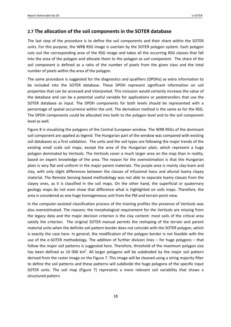
2.7 The allocation of the soil components in the SOTER database
The last step of the procedure is to define the soil components and their share within the SOTER units. For this purpose, the WRB RSG image is overlain by the SOTER polygon system. Each polygon cuts out the corresponding area of the RSG image and takes all the occurring RSG classes that fall into the area of the polygon and allocate them to the polygon as soil component. The share of the soil component is defined as a ratio of the number of pixels from the given class and the total number of pixels within the area of the polygon.
The same procedure is suggested for the diagnostics and qualifiers (DPDHs) as extra information to be included into the SOTER database. These DPDH represent significant information on soil properties that can be accessed and interpreted. This inclusion would certainly increase the value of the database and can be a potential useful variable for applications or pedotransfers that use the SOTER database as input. The DPDH components for both levels should be represented with a percentage of spatial occurrence within the unit. The derivation method is the same as for the RSG. The DPDH components could be allocated into both to the polygon level and to the soil component level as well.
Figure 8 is visualizing the polygons of the Central European window. The WRB RSGs of the dominant soil component are applied as legend. The Hungarian part of the window was compared with existing soil databases as a first validation. The units and the soil types are following the major trends of the existing small scale soil maps, except the area of the Hungarian plain, which represent a huge polygon dominated by Vertisols. The Vertisols cover a much larger area on the map than in reality, based on expert knowledge of the area. The reason for the overestimation is that the Hungarian plain is very flat and uniform in the major parent materials. The purple area is mainly clay‐loam and clay, with only slight differences between the classes of Infusional loess and alluvial loamy clayey material. The Remote Sensing based methodology was not able to separate loamy classes from the clayey ones, as it is classified in the soil maps. On the other hand, the superficial or quaternary geology maps do not even show that difference what is highlighted on soils maps. Therefore, the area is considered as one huge homogeneous unit from the PM and terrain point view.
In the computer‐assisted classification process of the training profiles the presence of Vertisols was also overestimated. The reasons: the morphological requirement for the Vertisols are missing from the legacy data and the major decision criterion is the clay content: most soils of the critical area satisfy the criterion. The original SOTER manual permits the reshaping of the terrain and parent material units when the definite soil pattern border does not coincide with the SOTER polygon, which is exactly the case here. In general, the modification of the polygon border is not feasible with the use of the e‐SOTER methodology. The addition of further division lines – for huge polygons – that follow the major soil patterns is suggested here. Therefore, threshold of the maximum polygon size has been defined as 10 000 km2. All larger polygons will be subdivided by the major soil pattern derived from the raster image on the Figure 7. This image will be cleaned using a string majority filter to define the soil patterns and these patterns will subdivide the huge polygons of the specific input SOTER units. The soil map (Figure 7) represents a more relevant soil variability that shows a structured pattern.
18

Report Deliverable No D5 e‐SOTER
The last step of the procedure is to define the soil components and their share within the SOTER units. For this purpose, the RSG image is overlain by the SOTER polygon system. Each polygon cuts out the corresponding area of the RSG image and takes all the occurring RSG classes that fall into the area of the polygon and allocate them to the polygon as soil component. The share of the soil component is defined as a ratio of the number of pixels from the given class and the total number of pixels within the area of the polygon.
The provisional SOTER database
Polygons Terrain and parent material based uniform units Bases for interpreting the environments, variables, stratification tool Easy way to visualize the major soil properties in a scale of 1:1M
Raster layers (90‐500m resolution) Terrain derivatives Texture classes Major diagnostic features relevant for the scale (likelihood) RSG of the WRB Raster layers are used to delineate the homogeneous landscape/physiographic unit
Maintained also as raster layers backing up the polygon database
Figure 8. The polygons of the CE window visualizing the WRB RSGs of the dominant soil components.
19

Report Deliverable No D5 e‐SOTER
3. Task 2.2 Compilation of a harmonized soil data base for the 1:1 million‐scale windows
The compilation of the harmonized soil data base needed 2 subtasks: the development of the revised
the soil component structure and the development of harmonization methodologies for the soil data
originating from the partner countries, produced and classified with various standards.
3. 1 The revised e‐SOTER data structure
The e‐SOTER database is derived from, and compatible with the Global Soil and Terrain (SOTER) database (van Engelen and Wen 1995). It is composed of a set of tables in a Relational Database Management System (RDBMS) linked to the geometric database (GIS file). The database is composed of various tables; the terrain, terrain component and soil component tables that describe the attributes of the spatial parts of SOTER, while the profile, horizon and WRB diagnostics describe the attributes of the profile (point) data. The e‐SOTER database has undergone a number of improvements in its structure, compared to the original SOTER database.
One of the major improvements has been the application of the updated standards for soil descriptions and soil classification. The master horizon designation, subordinate characteristics and site descriptions follow 2006 edition of the FAO Guidelines for soil description (FAO, 2006). The classification of soils and the related diagnostic horizons, properties and materials are described and coded according to the World Reference Base for soil recourses (IUSS Working Group WRB, 2006, 2007). All profiles (representative and reference) are given both the WRB classification, to link to new developments, and the classification according to the Revised Legend of the Soil Map of the World (FAO 1988) to link to the former SOTER databases. To facilitate for using SOTER as a profile database also parent material, land use and vegetation are given now in the profile table.
A new table, the WRB diagnostics, was included to describe properly the WRB diagnostic horizons, properties and materials as well as the depth of occurrence. All diagnostic horizon or property can apply for the same horizon and can be described. The qualifiers are listed together with the reference group.
Another improvement has been the inclusion of the small‐scale map legend using the World Reference Base for soil resources (addendum to WRB, 2010) in the soil component table. The WRB Legend and the Revised Legend (FAO 1988) are directly linked now to the geometric SOTER database and enable the user to derive various maps e.g. a dominant soil without too much database manipulation.
The legacy soil data from window partners were harmonized using the above standards. The data was loaded to the e‐SOTER database through the data entry mechanism (in access format) that is available on the on the team site.
20

Report Deliverable No D5 e‐SOTER
The availability and the completeness of the received data from the window partners was variable
and in several cases insufficient for proper correlation with the WRB.
The available profiles were mostly provided by the partner countries, additional profiles were
pooled from the WISE data base (Batjes, 2007). For the Central European window: 113 profiles from
Germany, 561 from the Czech Republic, 1247 from Hungary and 34 from Slovakia (not partner) were
available. For the Western European window the UK provided 92 profiles, France did not provide,
here 69 profiles were used from the WISE data base but only 9 of them fall into the window. For the
China window 210 and for the Morocco window 67 profile were collected. All together 2393 profiles
were harmonized and uploaded to the database.
3.3 Development of translation algorithms correlation tools for the
harmonization process All partners of the e‐SOTER project have different soil observation, analytical and classification systems and data management procedures. Beside the differences in standards in some cases even (Morocco, China) language was also a basic problem.
Figure 9. Agorithm to determine the calcic horizon from German soil data in the automated classification.
21

Report Deliverable No D5 e‐SOTER
For the harmonization and correlation several approaches were developed an exercised. The most logical approach is the translation of the data from one system to the other with translation algorithms. Eberhadt (BGR) and colleagues have been developing and testing translation algorithms for automated classification. The input data are legacy data recorded according to national systems and the output is the soil name according to WRB. Based on the testing withGerman data, the results are promising when the data set is complete. When the data are incomplete the system uses less reliable or less precise data fields (e. g. classed values instead of numbers). If less reliable data are used, the system logs detailed information to allow the expert to decide whether the results are reliable or not. An algorithm example is shown in Figure 9. The experiences with the development were published as basic research results (Eberhardt and Waltner , 2010). In the practical harmonization the approach was not applied yet, because the WRB (hence the system) requires data which are to a large extent not available in the received legacy data sets for the windows.
Another approach that was developed was the taxonomic distance‐based correlation. This approach was a modified method of the one introduced by Minasny and McBratney (2007). Taxonomic distances were calculated based on key “diagnostic” properties between national soil units and possible corresponding WRB classification units. The calculations were performed based on the classification concepts ‐ the required presence or exclusions of key properties ‐ and also based on actual data, by calculating the taxonomic distances with the centroids of soil classification units. Similarly to the first approach, the major limitation of applying the method was the lack of sufficient soil data for the calculations. The experiences with the development of methods were also published as basic research results (Láng et al, 2009, 2010; Waltner et al, 2010). In the applied practical harmonization and correlation process it was very important to consult with partner country experts and also the experiences of the soil correlation exercises which were organized to help the understanding of the classification system of the window countries.
In the received data sets, beside the original laboratory and some field observation data, in most
cases the WRB reference groups were provided. Diagnostics and qualifiers were provided only by the
Czech partner.
For all data sets a computer‐assisted determination of the diagnostics were applied with simplified
requirements of the WRB 2006. The simplification was adjusted to the availability of the required
information. The simplified classification algorithms that were run for the selected diagnostics that
were expected in the specific windows, are given in ANNEX 2.
In many cases even the simplified requirements were not available and expert judgment was used to determine the presence or absence of the diagnostics. Since many of the diagnostic features require morphological criteria, that are not part of the most legacy data sets, there are uncertainties in the diagnostic data sets.
Based on the diagnostics the WRB key was applied to determine the reference groups. The correlation results often did not match the WRB RSG given by the partners.
The expected qualifiers were also determined by simplified classification algorithms that were run for selected qualifiers, given in ANNEX III.
22

Report Deliverable No D5 e‐SOTER
The harmonized data are uploaded to the team site (Shared documents. WP2).
3. 4. Definition of representative profiles for soil components of the e‐SOTER
units
In the case when the polygon includes a reference profile for the RSG, it is considered to be the
representative profile. When more reference profiles are available for same RSG, the representative
profile is selected based on the followings: same parent material as the one defined for the SOTER
unit and having the same map unit qualifiers as the soil component.
When no reference profile occurs for the RSG in the SOTER unit, the spatially closest with same
parent material and qualifiers (as above) should be selected.
The definition of the representative profiles is in process.
References Batjes, N.H. 2009. Harmonized soil profile data for applications at global and continental scales:
updates to the WISE database. Soil Use and Management 25, 124‐127
Eberhardt Einear, Dana Pietsch: Classifying soils according to WRB with national soil legacy data,
Abstarct of the papers of the Conference “From the Dokuchaev School to numerical soil
classifications”, 18. September, 2009 Gödöllő, Hungary
Eberhardt, E.; Waltner, I., 2010: Finding a way through the maze – WRB classification with descriptive soil data. In: Gilkes, R. J. (ed.): 19th World Congress of Soil Science: Soil Solutions for a Changing World, 1‐6 August 2010, Brisbane, Australia. http://www.iuss.org/19th%20WCSS/symposium/pdf/1559.pdf
Eberhardt, E. and Waltner, I. Finding a way through the maze – WRB classification with descriptive
soil data 19th World Congress of Soil Science, 1‐6 August 2010, Brisbane, Australia, abstract
FAO 2006b. Guidelines for soil description. FAO, Rome, 97 p
IUSS Working Group WRB (2007) 'World reference base for soil resources 2006, update 2007, 2nd
ed.' World Soil Resources Reports 103. (FAO: Rome)
Láng, V., Fuchs, M., Waltner, I., Michéli, E.,2009: Correlation possibilities based on taxonomic
distance measurement. 25th SSSEA Conference, Moshi, Tanzania
Láng, V., Fuchs, M., Waltner, I., Michéli, E.,2010, Pedometrics application for correlation of Hungarian
soil types with WRB, 19. IUSS World Congress, Brisbane, Australia
Láng, V., Fuchs, M., Waltner, I., Michéli, E.,2010: Taxonomic distance measurements applied for soil
correlation, Agrokémia és Talajtan (in press).
Minasny, B., McBratney, A. B. 2007. Incorporating taxonomic distance into spatial prediction and
digital mapping of soil classes, Geoderma 142 (2007) 285‐293
23

Report Deliverable No D5 e‐SOTER
van Engelen VWP and Wen TT 1995. Global and National Soils and Terrain Digital Databases (SOTER),
Procedures Manual (revised edition), FAO, ISSS, ISRIC, Wageningen
Waltner, I., Láng, V., Fuchs, M. and Michéli, M. Application of a centroid‐based concept for the
correlation of national soil classification with the WRB 4th Global Workshop on Digital Soil
Mapping, 24‐26 May 2010 ‐ Rome, Italy, abstract
24

Report Deliverable No D5 e‐SOTER
ANNEX I: MODIS satellite images data sheet
• DOWNLOADING satellite data from MODIS server (e4ftl01u.ecs.nasa.gov).
o Downloaded composites:
MOD09A1.005
MOD11A2.005
o Downloaded tiles:
CE window:
• h18v03
• h18v04
• h19v03
• h19v04
UK/FR window:
• h17v03
• h17v04
• h18v03
• h18v04
MO window:
• h17v05
CH window:
• h28v06
• h28v07
• Downloaded dates. The downloaded dates should represent the vegetative period,
changing environmental conditions (like soil wetness, temperature) during the year,
cloud and snow‐free images from every second month are selected
CE window:
• 2008.02.02 – 2002.02.18
• 2009.04.15
• 2008.06.25
• 2008.08.28
25

Report Deliverable No D5 e‐SOTER
• 2006.10.16
UK/FR window:
• 2008.02.10
• 2004.04.22
• 2006.06.02
• 2003.08.05
• 2007.10.16
MO window:
• 2002.02.02
• 2008.04.30
• 2008.06.09
• 2007.08.21
• 2007.10.16
• 2000.12.10
CH window:
• 2008.02.26
• 2002.10.08
• 2008.12.02
• Images in hdf, hdf.xml format
• IMPORTING images from hdf to img format with ERDAS Imagine
• LAYER SELECTION:
o From MOD09A1: Band 1‐7 (Layers 1‐7)
o From MOD11A2: Band 31‐32 (Layers 9‐10), LST (Land Surface Temperature) Day
(Layer 1) and LST Night (Layer 5)
• LAYER STACK: The above mentioned layers were stacked with ERDAS Imagine with the
resolution and the output type of the finer resolution image (MOD09A1). The result is a 11
layer, 500 meter image.
o Layer 1: Band 1
o Layer 2: Band 2
o Layer 3: Band 3
o Layer 4: Band 4
o Layer 5: Band 5
26

Report Deliverable No D5 e‐SOTER
o Layer 6: Band 6
o Layer 7: Band 7
o Layer 8: LST Day
o Layer 9: LST Night
o Layer 10: Band 31
o Layer 11: Band 32
• MOSAICING the four tiles for each date, and layer stacking all the channels of all dates, which
results a usually 33‐55‐66 layer image depending on the number of cloud‐free and snow‐free
dates.
• PCA: Principal component analysis (PCA) was run on the images to reduce the number of
layers and the first 15 channels were kept.
• LST: A normalized temperature fluctuation layer was created for each dates using the
following function: globmax(lstday)/lstday*(LST Day‐LST Night)
• BAND RATIOS FROM THE LITERATURE (ORIGINALLY FOR LANDSAT):
o 6/1
o 1/3
o 7/6
27

Report Deliverable No D5 e‐SOTER
ANNEX II. The simplified criteria for the expected WRB diagnostics Diagnostic horizons Albic horizon 1. Munsell colour (dry) with either:
a. a value of 7 or 8 and a chroma of 3 or less; or b. a value of 5 or 6 and a chroma of 2 or less; and 2. Munsell colour (moist) with either: a. a value of 6, 7 or 8 and a chroma of 4 or less; or b. a value of 5 and a chroma of 3 or less; or c. a value of 4 and a chroma of 2 or less; and 3. thickness of 1 cm or more;
Argic horizon 1. if the overlying horizon has < 15% clay, at least 3 percent more clay content increase in the underlying horizon; or 2. if the overlying horizon has a clay content between 15‐40%, the ratio of clay in the underlying to that of the overlying horizon must be 1.2 or more; or 3. if the overlying horizon has > 40% or more clay, the underlying horizon must contain at least 8 percent more clay; or 4. morphological evidence of clay illuviation in soil description (i.e. cutanic qualifier); and 5. does not form part of a natric horizon.
Calcic horizon 1. calcium carbonate content > 15%; and 2. thickness > 15 cm; and 3. > 5% secondary carbonates (if data available).
Cambic horizon 1. has a texture of loamy sand or finer; and 2. has soil structure (rock structure, massive and single grain structure type are excluded); and 3. has a thickness > 15 cm; and 5. has higher Munsell chroma or value (moist), or redder Munsell hue, or higher clay content than the underlying or an overlying layer; or 6. lower carbonate content than the underlying horizon.
Ferralic horizon 1. has a texture of sandy loam or finer; and 2. CaCO3 content < 5%; and 3. OC between 1,4‐20%; and 4. CEC < 4 cmol/kg 5. has a thickness > 30 cm; and 6. does not form part of C or R horizon.
Folic horizon 1. OC > 20%; and 2. has a thickness > 10 cm; and 3. does not form part of an H horizon.
Gypsic horizon 1. > 5% gypsum content; and 2. a product of thickness (in centimetres) times gypsum content (percentage) > 150; and 3. a thickness > 15 cm.
Histic horizon 1. OC > 20%; and 2. has a thickness > 10 cm,
28

Report Deliverable No D5 e‐SOTER
3. does not form part of a folic horizon.
Mollic horizon 1. OC > 0,6%; and 2. a Munsell value (moist) of 3 and a chroma (moist) of 3 or less; and 3. a Munsell value (dry) of 5 and a chroma (dry) of 5 or less (if data available); and 4. B% > 50; and 5. a thickness > 25 cm; or 6. a thickness > 10 cm if directly overlying continuous rock; and 7. surface horizon.
Natric horizon 1. satisfy the criteria of argis horizon; and 2. ESP (exchangeable Na percentage) > 15.
Nitic horizon 1. clay content > 30%; and 2. a silt to clay ratio less than 0,4; and 3. thickness > 30 cm; and 4. moderate or strong structure (if data available).
Salic horizon 1. EC (electrical conductivity of the saturation extract) > 15 dS m‐1; or 2. EC > 8 dS m‐1 if pH > 8,5; 3. thickness > 15 cm.
Spodic horizon 1. pH < 5,9; and 2. OC > 0,5%; and 3. Munsell hue 5 YR or redder; or 4. a Munsell hue of 7.5 YR with a value of 5 or less and a chroma of 4 or less; or 5. a Munsell hue of 10 YR or neutral and a value and a chroma of 2 or less; or 6. a colour of 10 YR 3/1; or 7. horizon designation is Bh, Bs or Bhs,and 8. does not form part of C or R horizon.
Umbric horizon 1. OC > 0,6%; and 2. a Munsell value (moist) of 3 and a chroma (moist) of 3 or less; and 3. a Munsell value (dry) of 5 and a chroma (dry) of 5 or less (if data available); and 4. B% < 50; and 5. a thickness > 25 cm; or 6. a thickness > 10 cm if directly overlying continuous rock; and 7. surface horizon.
Vertic horizon 1. clay content > 30%; and 2. has a thickness > 25 cm.
Voronic horizon 1. OC > 1,5%; and 2. a Munsell value (moist) of 2 and a chroma (moist) of 2 or less; and 3. a Munsell value (dry) of 3 and a chroma (dry) of 3 or less (if data available); and 4. B% > 80; and 5. a thickness > 35 cm; and 6. surface horizon.
29

Report Deliverable No D5 e‐SOTER
Diagnostic properties Abrupt textural change
1. if the overlying horizon has < 20% clay, doubling of the clay content; or 2. if the overlying horizon has > 20% clay, 20% increase in clay content; and 3. distinctness of horizon transition is abrupt or clear.
Albeluvic tonguing
If RSG is Albeluvisol
Andic properties 1. Bulk density < 0,9 g/cm3; and 2. OC < 25%; and 3. does not form part of organic material.
Continuous rock 1. parent material is hard rock; and 2. shallow profile (lower horizon boundary of the deepest horizon < 1 m); or
3.profile contanins just 1 sampled horizon; or 4. coarse framents > 80%; or 5. horizon designation is R.
Gleyic colour pattern
1. Munsell hue N1/ to N8/ or 2.5 Y, 5 Y, 5 G, 5 B; or 2. Subordinate characteristics of horizon designation consists of „g” or „l” or other symbol refers to gleyic colour pattern; or 3. Depth to groundwater < 1 m; or 4. Poorly or very poorly drained.
Lithological discontinuity
The difference in sand or coarse fragment content between the underlying to that of the overlying horizon must be 10 or more.
Reducing conditions
Subordinate characteristics of horizon designation consists of „r” or other symbol refers to reducing conditions.
Secondary carbonates
Presence of carbonate concretions (in soil description).
Stagnic colour pattern
Subordinate characteristics of horizon designation consists of „g” or other symbol refers to stagnic colour pattern.
Diagnostic materials Artefacts If RSG is Technosol
Calcaric material 1. CaCO3 content > 2%; and 2. does not form part of a calcic horizon.
Colluvic material No data
Fluvic material 1. Presence of lithological discontinuity; and 2. OC is more than that of the overlying horizon.
Organic material OC > 20%
Technic hard rock
No data
30

Report Deliverable No D5 e‐SOTER
ANNEX III. The simplified set of criteria for the expected WRB qualifiers Qualifiers Acric 1. Having an argic horizon that has a CEC < 24 cmolc kg‐1 clay; and
2. having a base saturation < 50% between 50 and 100 cm from the soil surface.
Albic Having an albic horizon starting within 100 cm of the soil surface.
Andic Having andic properties in a thickness of 30 cm or more, starting within 100 cm of the soil surface.
Arenic Having a texture of loamy sand or coarser in a layer, 30 cm or more thick, within 100 cm of the soil surface.
Calcaric Having calcaric material between 20 and 50 cm from the soil surface.
Calcic Having a calcic horizon or concentrations of secondary carbonates starting within 100 cm of the soil surface.
Cambic Having a cambic horizon starting within 50 cm of the soil surface.
Clayic Having a texture of clay in a layer, 30 cm or more thick, within 100 cm of the soil surface.
Cutanic Presence of clay skins (in soil description).
Dystric Having a B% < 50% between 20 and 100 cm from the soil surface or between 20 cm and continuous rock.
Eutric Having a B% > 50% between 20 and 100 cm from the soil surface or between 20 cm and continuous rock.
Fluvic Having fluvic material in a layer, 25 cm or more thick, within 100 cm of the soil surface.
Gleyic Having gleyic colour pattern within 100 cm of the soil surface.
Haplic Only used if none of the preceding qualifiers applies.
Histic Having a histic horizon starting within 40 cm of the soil surface.
Humic 1. In Ferralsols and Nitisols: weighted average of OC > 1,4% to a depth of 100 cm from the mineral soil surface; 2. In Leptosols: weighted average of OC > 2% to a depth of 25 cm from the mineral soil surface; 3. In other soils: weighted average of OC > 1% to a depth of 50 cm from the mineral soil surface.
Leptic Having continuous rock starting within 100 cm of the soil surface.
Lithic Having continuous rock starting within 10 cm of the soil surface (in Leptosols only).
Luvic 1. Having an argic horizon that has a CEC < 24 cmolc kg‐1 clay; and 2. having a base saturation > 50% between 50 and 100 cm from the soil
31

Report Deliverable No D5 e‐SOTER
surface.
Mollic Having a mollic horizon.
Natric Having a natric horizon starting within 100 cm of the soil surface.
Rendzic Having a mollic horizon that immediately overlies calcareous rock or calcareous material containing CaCO3 > 40%.
Salic Having a salic horizon starting within 100 cm of the soil surface.
Skeletic Having > 40% gravel or other coarse fragments averaged over a depth of 100 cm from the soil surface or to continuous rock, whichever is shallower.
Sodic Having exchangeable Na plus Mg > 15% within 50 cm of the soil surface.
Spodic Having a spodic horizon starting within 200 cm of the mineral soil surface.
Stagnic Having stagnic colour pattern within 100 cm of the soil surface.
Umbric Having an umbric horizon.
Vertic Having a vertic horizon starting within 100 cm of the soil surface.
32