1

A soft soil model that accounts for creep

P.A. Vermeer & H.P. NeherInstitute of Geotechnical Engineering, University of Stuttgart, Germany

Keywords: aging, creep, consolidation, soft soil

ABSTRACT: The well-known logarithmic creep law for secondary compression is transformedinto a differential form in order to include transient loading conditions. This 1-D creep model foroedometer-type strain conditions is then extended towards general 3-D states of stress and strain byincorporating concepts of Modified Cam-Clay and viscoplasticity. Considering lab test data it isshown that phenomena such as undrained creep, overconsolidation and aging are well captured bythe model.

1 INTRODUCTION

As soft soils we consider near-normally consolidated clays, clayey silts and peat. The special fea-tures of these materials is their high degree of compressibility. This is best demonstrated byoedometer test data as reported for instance by Janbu in his Rankine lecture (1985). Consideringtangent stiffness moduli at a reference oedometer pressure of 100 kPa, he reports for normally con-solidated clays Eoed = 1 to 4 MPa, depending on the particular type of clay considered. The differ-ences between these values and stiffnesses for NC-sands are considerable as here we have values inthe range of 10 to 50 MPa, at least for non-cemented laboratory samples. Hence, in oedometertesting normally consolidated clays behave ten times softer than normally consolidated sands. Thisillustrates the extreme compressibility of soft soils.

Another feature of the soft soils is the linear stress-dependency of soil stiffness. According to

the Hardening-Soil model we have Eoed = Eoedref �1���p ref)m , at least for c = 0, and a linear relation-

ship is obtained for m = 1. Indeed, on using an exponent equal to one, the above stiffness law re-

duces to Eoed = 1 / �*, where �* = pref / Eoedref . For this special case of m = 1, the Hardening-Soil

model yields 0� = �* /11� , which can be integrated to obtain the well-known logarithmic compres-sion law 0 = �* ln1 for primary oedometer loading. For many practical soft-soil studies, the modi-fied compression index �* will be known and we can compute the oedometer modulus from the re-

lationship Eoedref = pref / �*.

From the above considerations it would seem that the HS-model is perfectly suitable for softsoils. Indeed, most soft soil problems can be analysed using this model, but the HS-model is notsuitable when considering creep, i.e. secondary compression. All soils exhibit some creep, and pri-mary compression is thus always followed by a certain amount of secondary compression. Assum-ing the secondary compression (for instance during a period of 10 or 30 years) to be a small per-centage of the primary compression, it is clear that creep is important for problems involving largeprimary compression. This is for instance the case when constructing road or river embankmentson soft soils. Indeed, large primary settlements of dams and embankments are usually followed bysubstantial creep settlements in later years.

In some cases dams or buildings may also be founded on initially overconsolidated soil layersthat yield relatively small primary settlements. Then, as a consequence of the loading, a state ofnormal consolidation may be reached and significant creep may follow. This is a treacherous situa-

2

tion as considerable secondary compression is not preceeded by the warning sign of large primarycompression.

Apart from foundation-related problems, creep plays an important role in steep slopes. Manynatural slopes have a relatively small factor of safety and they show continuous displacements dueto creep. Gradual geometric changes and associated degradation of strength may then lead to slopeslides. The various different problems that relate to creep have motivated us to develop a stress-strain relationship that takes creep into account.

Buisman (1936) was probably the first to propose a creep law for clay after observing that soft-soil settlements could not be fully explained by classical consolidation theory. The work on 1D-secondary compression was continued by researchers including, for example, Bjerrum (1967),Garlanger (1972) and Mesri (1977) and Leroueil (1977). A more mathematical lines of research inthe area were followed by, for example, Sekiguchi (1977), Adachi and Oka (1982) and Borja et al.(1985). This line of mathematical 3D-creep modelling was influenced by the more experimentalline of 1D-creep modelling, but conflicts exist.

From the authors viewpoint, 3D-creep should be a straight forward extension of 1D-creep, butthis is hampered by the fact that present 1D-models have not been formulated as differential equa-tions. For the presentation of the Soft-Soil-Creep model we will first complete the line of 1D-modelling by conversion to a differential form, from which an extension is made to a 3D-model. Inaddition, attention is focused on the model parameters. Finally the model will be validated by con-sidering both model predictions and data from triaxial tests. Here attention is focused on constantstrain-rule shear tests and undrained creep tests.

2 BASICS OF ONE-DIMENSIONAL CREEP

When reviewing previous literature on secondary compression in oedometer tests, one is struck bythe fact that it concentrates on behaviour related to step loading even though natural loading proc-esses tend to be continuous or transient in nature. Buisman (1936) who was probably the first toconsider such a classical creep test. He proposed the following to describe creep behaviour underconstant effective tress,

c Bc

c = + C t

t t tε ε log for > (1)

where 0c is the strain up to the end of consolidation, t the time measured from the beginning ofloading, tc the time to the end of primary consolidation and CB is a material constant. As is often thecase in soil mechanics, compression is assumed to be positive. For further consideration, it is con-venient to rewrite this equation as

ε ε = + C t + t

t tc B

c

clog for >

′ ′ 0 (2)

with t� = t - tc being the effective creep time.Based on the work by Bjerrum on creep, as published for instance in 1967, Garlanger (1972),

proposed a creep equation of the form

e = e - C + t

C C e tcc

cBα α

ττ

log with = ( + ) > ′ ′1 00 for (3)

Differences between Garlanger s and Buisman s forms are modest. The engineering strain 0 is re-placed by void ratio e and the consolidation time tc is replaced by a parameter 2c. Equations (2) and(3) are entirely identical when choosing 2c = tc. For the case that 2c g tc differences between bothformulations will vanish when the effective creep time t increases.

For practical consulting, oedometer tests are usually interpreted by assuming tc = 24 h. Indeed,the standard oedometer test is a Multiple Stage Loading Test with loading periods of precisely oneday. Due to the special assumption that this loading period coincides to the consolidation time tc, it

3

follows that such tests have no effective creep time. Hence one obtains t� = 0 and the log-termdrops out of equation (3). It would thus seem that there is no creep in this standard oedometer test,but this suggestion is entirely false. Even highly impermeable oedometer samples need less thanone hour for primary consolidation. Then all excess pore pressures are zero and one observes purecreep for the other 23 hours of the day. Therefore we will not make any assumptions about the pre-cise values of 2c and tc.

Another slightly different possibility to describe secondary compression is the form adopted byButterfield (1979)

HcH c

c = + C

+ tε ε τ

τln

′(4)

where 0H is the logarithmic strain defined as

H

o o = -

V

V = -

1+ e

1+ eε ln ln (5)

with the subscript !o denoting the initial values. The superscript !H is used for denoting logarith-mic strain. We use this particular symbol, as the logarithmic strain measure was originally used byHencky. For small strains it is possible to show that

C = C

+ e =

C

o

Bα1 10 100 5 ⋅ ln ln

(6)

because then logarithmic strain is approximately equal to the engineering strain. Both Butterfield(1979) and Den Haan (1994) showed that for cases involving large strain, the logarithmic smallstrain supersedes the traditional engineering strain.

3 ON THE VARIABLES τC AND εC

In this section attention will first be focussed on the variable 2c. Here a procedure is to be describedfor an experimental determination of this variable. In order to do so we depart from equation (4).By differentiating this equation with respect to time and dropping the superscript !H to simplifynotation, one finds

� or inversely 1�

= + ε

τ ετ

= C

+ t

t

Cc

c

′′

(7)

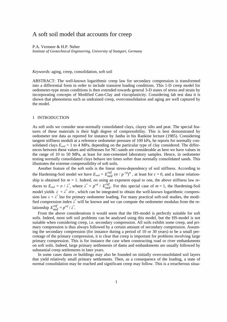
which allows one to make use of the construction developed by Janbu (1969) for evaluating theparameters C and 2c from experimental data. Both the traditional way, being indicated in Figure 1a,as well as the Janbu method of Figure 1b can be used to determine the parameter C from anoedometer test with constant load. The use of the Janbu method is attractive, because both 2c and Cfollow directly when fitting a straight line through the data. In Janbu s representation of Figure 1b,

Figure 1. Consolidation and creep behaviour in standard oedometer test.

4

2c is the intercept with the (non-logarithmic) time axis of the straight creep line. The deviation froma linear relation for t < tc is due to consolidation.

Considering the classical literature it is possible to describe the end-of-consolidation strain 0c,by an equation of the form

c ce

cc pc

p = + = A + B ε ε ε

σσ

σσ

ln ln′′0 0

(8)

Note that� 0 is a logarithmic strain, rather than a classical small strain although we convenientlyomit the superscript !H . In the above equation 10� represents the initial effective pressure beforeloading and 1� is the final effective loading pressure. The values 1p0 and 1pc representing the precon-solidation pressure corresponding to before-loading and end-of-consolidation states respectively. Inmost literature on oedometer testing, one adopt e instead of 0, and log instead of ln, and the swel-ling index Cr instead of A, and the compression index Cc instead of B. The above constants A and Brelate for small strains to Cr and Cc as

A = C

+ e B =

C C

+ e r

o

c r

o1 10 1 100 50 5

0 5⋅ ⋅ln ln(9)

Combining equations (4) and (8) it follows that

ε ε εσσ

σ

στ

τ = + = A + B + C

+ te c pc

p

c

cln ln ln

′′

′

0 0(10)

where 0 is the total logarithmic strain due to an increase in effective stress from 10� to 1� and a timeperiod of tc+t � . In Figure 2 the terms of equation (10) are depicted in a 0�ln1 diagram.

Up to this point, the more general problem of creep under transient loading conditions has notyet been addressed, as it should be recalled that restrictions have been made to creep under constantload. For generalising the model, a differential form of the creep model is needed. No doubt, such ageneral equation may not contain t� and neither�2c as the consolidation time is not clearly defined fortransient loading conditions.

4 DIFFERENTIAL LAW FOR 1D-CREEP

The previous equations emphasize the relation between accumulated creep and time, for a givenconstant effective stress. For solving transient or continuous loading problems, it is necessary toformulate a constitutive law in differential form, as will be described in this section. In a first stepwe will derive an equation for 2c. Indeed, despite the use of logarithmic strain and ln instead of log,the formula (10) is classical without adding new knowledge. We may also deviate a bit as we write

Figure 2. Idealised stress-strain curve from oedometer test with division of strain increments into an elasticand a creep component. For t� + tc = 1 day one arrives precisely on the NC-line.

5

1pc when some other authors write 1�. Moreover, the question on the physical meaning of 2c is stillopen. In fact, we have not been able to find precise information on 2c, apart from Janbu s method ofexperimental determination.

In order to find an analytical expression for the quantity 2c, we adopt the basic idea that all ine-lastic strains are time dependent. Hence total strain is the sum of an elastic part 0

e and a time-dependent creep part 0

c. For non-failure situations as met in oedometer loading conditions, we donot assume an instantaneous plastic strain component, as used in traditional elastoplastic modelling.In addition to this basic concept, we adopt Bjerrum s idea that the preconsolidation stress dependsentirely on the amount of creep strain being accumulated in the course of time. In addition to equa-tion (10) we therefore introduce the expression

ε ε ε σσ

σσ

σ σ ε= + ′′

+ → =�

���

��e c p

pp p

c = A B

Bln ln exp

0 00 (11)

The longer a soil sample is left to creep the larger 1p grows. The time-dependency of the precon-solidation pressure 1p is now found by combining equations (10) and (11) to obtain

c cc

p

pc

c

c- = B = C

+ tε ε

σσ

ττ

ln ln′

(12)

This equation can now be used for a better understanding of 2c, at least when adding knowledgefrom standard oedometer loading. In conventional oedometer testing the load is stepwise increasedand each load step is maintained for a constant period of tc+t �� �2 , where 2 is precisely one day. Inthis way of stepwise loading the so-called normal consolidation line (NC-line) with 1p� �1� is ob-tained. On entering 1p� �1� and t�� �2��Wc into equation (12) it is found that

B = C + - t

pc

c c

cln ln for OCR = 1

′σσ

τ ττ

(13)

It is now assumed that (2c - tc) Q�2. This quantity can thus be disregarded with respect to 2�and itfollows that

ττ

σσ

τ τσσc

B

C

pcc

B

Cpc = =

′�

���

�� ′���

���

or (14)

Hence 2c depends both on the effective stress 1� and the end-of-consolidation preconsolidationstress 1pc. In order to verify the assumption (2c - tc) Q 2, it should be realised that usual oedometersamples consolidate for relatively short periods of less than one hour. Considering load steps on thenormal consolidation line, we have OCR = 1 both in the beginning and at the end of the load step.During such a load step 1p increases from 1p0 up to 1pc during the short period of (primary) consoli-dation. Hereafter 1p increases further from 1pc up to�1� during a relatively long creep period. Hence,at the end of the day the sample is again in a state of normal consolidation, but directly after theshort consolidation period the sample is under-consolidated with 1p���1� . For the usually very highratios of B/C � 15, we thus find very small 2c-values from equation (14). Hence not only tc but also2c tend to be small with respect to 2� It thus follows that the assumption (2c - tc) Q 2 is certainly cor-rect.

Having derived the simple expression (14) for 2c, it is now possible to formulate the differentialcreep equation. To this end equation (10) is differentiated to obtain

� � ��

ε ε εσσ τ

= + = A + C

+ te c

c

′′ ′

(15)

where�2c+ t' can be eliminated by means of equation (12) to obtain

6

� � ��

with = expε ε εσσ τ

σσ

σ σ ε = + = A +

C

Be c

c

B

Cpc

pp p

c′′

�

���

�����

���0 (16)

Equation (14) can now be introduced to eleminate 2c and 1pc and to obtain

� � ��

where = expε ε εσσ τ

σσ

σ σ ε = + = A +

C

Be c

B

C

pp p

c′′

′�

���

�����

���0 (17)

5 THREE-DIMENSIONAL-MODEL

On extending the 1D-model to general states of stress and strain, the well-known stress invariantsfor pressure S� �1oct and deviatoric stress q = 32oct/�2 are adopted, with 1oct and 2oct being the octa-hedral normal and shear stresses respectively. These invariants are used to define a new stressmeasure named peq:

eq2

2p = p +

q

M p′

′(18)

with = + + and = - + - + -′ ′ ′ ′p q1

3

1

21 2 3

21 2

21 3

22 3σ σ σ σ σ σ σ σ σ0 5 0 5 0 5 0 5

In Figure 3 it is shown that the stress measure peq is constant on ellipses in p-q-plane. In fact wehave the ellipses from the Modified Cam-Clay-Model as introduced by Roscoe and Burland (1968).The soil parameter M represents the slope of the so-called !critical state line as also indicated inFigure 3. We use the above equation for the deviatoric stress q and

M = 6

3cv

cv

sin

sin

ϕϕ

(19)

where Qcv is the critical-void friction angle, also referred to as critical-state friction angle. On usingthe above definition for q, the equivalent pressure peq is constant along ellipsoids in principal stressspace. To extend the 1D-theory to a general 3D-theory, attention is now focused on normally con-solidated states of stress and strain as met in oedometer testing. In such situations it yields12�� �13� = K0,NC

11� , and it follows from equation (18) that

Figure 3. Diagram of peq-ellipse in a p-q-plane.

7

eqNC NC

NC

peq

p

NC NC

NC

p = + K

+ - K

M + K

p = + K

+ - K

M + K

′�

!

"

$

##

�

!

"

$

##

σ

σ

1 2

3

3 1

1 2

1 2

3

3 1

1 2

02

02

0

02

02

0

2 7

2 7

2 7

2 7

(20)

where 1� �11� , and ppeq is a generalised preconsolidation pressure, being simply proportional to the

one-dimensional one. For known values of K NC0 , peq can thus be computed from 1� and pp

eq can

thus be computed from� 1p. Omitting the elastic strain in the 1D-equation (17), introducing the

above expressions for peq and ppeq and writing 0v instead of 0 it is found that

vc

B

Ceq

peq p

eqpeq v

c =

C p

p p p

B� where = expε

τε�

��

�

��

���

���0 (21)

For one-dimensional oedometer conditions, this equation reduces to equation (17), so that one has atrue extension of the 1D-creep model. It should be noted that the subscript !0 is once again used inthe equations to denote initial conditions and that εv

c = 0 for time t = 0.Instead of the parameters A, B and C of the 1D-model, we will now change to the material pa-

rameters �*, �* and �*, who fit into the framework of critical state soil mechanics. Conversion be-tween constants follows the rules

* ur

ur

* * * -

+ A , B = - , = Cκ

νν

λ κ µ≈3 1

1

0 50 5

(22)

On using these new parameters, equation (21) changes to become

vc

* -

eq

peq p

eqpeq v

c

* * =

p

p , p = p

-

* *

*

� expεµτ

ελ κ

λ κµ�

��

�

��

���

���0 (23)

As yet the 3D-creep model is incomplete, as we have only considered a volumetric creep strain εvc ,

whilst soft soils also exhibit deviatoric creep strains. For introducing general creep strains, weadopt the view that creep strain is simply a time-dependent plastic strain. It is thus logic to assumea flow rule for the rate of creep strain, as usually done in plasticity theory. For formulating such aflow rule, it is convenient to adopt the vector notation

σ σ σ σ ε ε ε ε = , , T T1 2 3 1 2 30 5 0 5and = , ,

where T is used to denote a transpose. Similar to the 1D-model we have both elastic and creepstrains in the 3D-model. Using Hook s law for the elastic part, and a flow rule for the creep part,one obtains

� � � �ε ε ε σ λσ

= + = D + ge c -1

c′ ∂

∂ ′(24)

where the elasticity matrix and the plastic potential function are defined as

8

-

ur

ur ur

ur ur

ur ur

c eqD = E

- -

- -

- -

g p1 11

1

1

ν ν

ν ν

ν ν

�

!

"

$

###

and =

Hence we use the so-called equivalent pressure peq as a plastic potential function for deriving theindividual creep strain-rates components. The superscripts !ur are introduced to emphasize thatboth the elasticity modulus and Poisson s ratio will determine unloading-reloading behaviour. Nowit follows from the above equations that

vc c c c

eq eq eq eq

p = + + =

p +

p +

p =

p� � � �ε ε ε ε λ

σ σ σλ1 2 3

1 2 3

∂∂ ′

∂∂ ′

∂∂ ′

�

���

��∂

′∂(25)

+HQFH�ZH�GHILQH�.� �∂ ′∂peqp/ . Together with equations (23) and (24) this leads to

� ��

�ε σ εα σ

σα

µτ σ

λ κµ

= D + p

= D + p

p

p- vc eq

-*

- eq

peq

eq

* *

*1 1 1′ ∂

∂ ′′

�

��

�

��

∂∂ ′

(26)

where = exp -

or inversely = - ln * ** *

peq

peq v

c

vc p

eq

peq

p pp

p00

ελ κ

ε λ κ���

���

2 7

6 FORMULATION OF ELASTIC 3D-STRAINS

Considering creep strains, it has been shown that the 1D-model can be extended to obtain the 3D-model, but as yet this has not been done for the elastic strains. To get a proper 3D-model for theelastic strains as well, the elastic modulus Eur has to been defined as a stress-dependent tangentstiffness according to

ur ur ur ur *E = 3 1- 2 K = 3 1- 2 p

ν νκ

0 5 0 5′

(27)

Hence, Eur is not a new input parameter, but simply a variable quantity that relates to the input pa-rameter �*. On the other hand vur is an additional true material constant. Hence similar to Eur, thebulk modulus Kur is stress dependent according to the rule Kur = p�����*. Now it can be derived forthe volumetric elastic strain that

ve

ur

*ve =

p

K =

p

p

p

p�

� �or by integration = ln*ε κ ε κ

′ ′′

′′0

(28)

Hence in the 3D-model the elastic strain is controlled by the mean stress p� , rather than by principalstress 1� as in the 1D-model. However mean stress can be converted into principal stress. For one-

dimensional compression on the normal consolidation line, we have both 3p� = (1+2 K NC0 )1� and

3p0� = (1+2 K NC0 )10� and it follows that p� /p0� �1���10. As a consequence we derive the simple rule

ενe� �* ln(1���10� ), whereas the 1D-model involves εν

e =A ln(1���10� ). It would thus seem that �* co-

incides with A. Unfortunately this line of thinking can not be extended towards overconsolidatedstates of stress and strain. For such situations, it can be derived that

� �′′

′′

p

p =

1 +

1 -

1

1 + 2K ur

ur 0

νν

σσ

(29)

9

and it follows that

ve * ur

ur

*

0 =

p

p =

1 +

1 -

1 + 2K �

� �

ε κ νν

κ σσ

′′

′′

(30)

where K0 depends to a great extend on the degree of overconsolidation. For many situations, it isreasonable to assume K0 � 1 and together with vur � 0.2 one obtains 2εν

e � �* ln(1�� �10� ). Good

agreement with the 1D-model is thus found by taking �* � 2A.

7 REVIEW OF THE MODEL PARAMETERS

As soon as the failure yield criterion f (1�, c, Q) = 0 is met, instantaneous plastic strain rates developaccording to the flow rule �ε p

���0g/01� with g = g (1����%). This gives as additional soil parametersthe effective cohesion, c, the Mohr-Coloumb friction angle, Q, and the dilatancy angle %. For finegrained, cohesive soils, the dilatancy angle tends to be small, it may often be assumed that % isequal to zero. In conclusion, the Soft-Soil-Creep model requires the following material constants.

Failure parameters as in the Mohr-Coulomb model:

c : Cohesion [kN/m2]Q : Friction angle [°]% : Dilatancy angle [°]

Parameters of the Soft-Soil-Creep model:

�* : Modified swelling index [-]�* : Modified compression index [-]�* : Modified creep index [-]vur : Poisson's ratio for unloading-reloading [-]M : Slope of the so-called !critical state line [-]

7.1 Modified swelling index, modified compression index and modified creep index

These parameters can be obtained both from an isotropic compression test and an oedometer test.When plotting the logarithm of stress as a function of strain, the plot can be approximated by twostraight lines (see Figure 2). The slope of the normal consolidation line gives the modified com-pression index �*, and the slope of the unloading (or swelling) line can be used to compute themodified swelling index �*, as explained in section 6. Note that there is a difference between themodified indices �* and �* and the original Cam-Clay parameters � and �. The latter parameters aredefined in terms of the void ratio e instead of the volumetric strain 0v. The parameter �* can be ob-tained by measuring the volumetric strain on the long term and plotting it against the logarithm oftime (see Figure 1).

Relationship to Cam-Clay parameters:

* * = 1 + e

= 1 + e

λλ

κκ

(31)

Relationship to internationally normalized parameters:

* c * ur

ur

r *C. ( + e)

.

-

+

C + e

=C

. ( + e )λ κ ν

νµ α= ≈

2 3 1

3

2 3

1

1 1 2 3 1(32)

As already indicated in section 6, there is no exact relation between the isotropic compression indi-ces � and �* and the one-dimensional swelling index Cr, because the ratio of horizontal and vertical

10

stress changes during one-dimensional unloading. For the approximation it is assumed that the av-erage stress state during unloading is an isotropic stress state, i.e. horizontal and vertical stressequal.

For a rough estimate of the model parameters, one might use the correlation �*� Ip (%) / 500, the

fact that �*/�* is in the range between 15 to 25 and the general observation �*/�* is in the rangebetween 5 to 10.

For characterising a particular layer of soft soil, it is also necessary to know the initial pre-consolidation pressure 1p0. This pressure may e.g. be computed from a given value of the overcon-solidation ratio (OCR). Subsequently 1p0 can be used to compute the initial value of the generalisedpreconsolidation pressure pp

eq.

7.2 Poisson's ratio

In the case of the Soft-Soil-Creep model, Poisson's ratio is purely an elasticity constant rather thana pseudo-elasticity constant as used in the Mohr-Coulomb model. Its value will usually be in therange between 0.1 and 0.2. For loading of normally consolidated materials, Poisson's ratio plays aminor role, but it becomes important in unloading problems. For example, for unloading in a one-dimensional compression test (oedometer), the relatively small Poisson's ratio will result in a smalldecrease of the lateral stress compared with the decrease in vertical stress. As a result, the ratio ofhorizontal and vertical stress increases, which is a well-known phenomenon for overconsolidatedmaterials. Hence, Poisson's ratio should be based on the ratio of difference in horizontal stress todifference in vertical stress in oedometer unloading and reloading.

ur

ur

xx

yy - =

ν

νσσ1

∆∆

(33)

8 VALIDATION OF THE 3D-MODEL

This section briefly compares the simulated response of undrained triaxial creep behaviour ofHaney clay with test data provided by Vaid and Campanella (1977), using the material parameterssummarized in Table 1. A extensive validation is provided in Stolle et al.(1997). All triaxial testsconsidered were completed by initially consolidating the samples under an effective isotropic con-fining pressure of 525 kPa for 36 hours and then allowing them to stand for 12 hours underundrained conditions before starting the shearing part of the test.

The end-of-consolidation preconsolidation pressure just before shearing, ppceq, was found to be

373 kPa. This value was determined by simulating the consolidation part of the test. The precon-

solidation pressure ppceq of 373 kPa is less than 525 kPa, which would have been required for an

OCRo of 1. It is clear that the preconsolidation pressure not only depends on the applied maximumconsolidation stress, but also on time as discussed in previous section. In Figure 4 we can see theresults of Vaid and Campanella s tests (1977) for different strain rates and the computed curves,that were calculated with the present creep model. It is observed that the model describe the testsvery well.

Table 1. Material properties for Haney clay.

�* = 0.016 �* = 0.105 �* = 0.004v = 0.253mc = 32o %� ��o c = 0 kPa3cs = 32.1o

11

Figure 4. Results of the undrained triaxial tests (CU-tests) with different rates of strain. The faster the test thehigher the undrained shear strength.

Figure 5. Strain rate dependency of the effective stress path in undrained triaxial tests.

8.1 Constant strain rate shear tests

Undrained triaxial compression tests, as considered in Figure 4, are performed under constant ratesof vertical strain �ε1 and constant horizontal pressure 13, so the vertical stress 11 is allowed to in-crease. In the range of classical triaxial compression tests the shear stress q, for different strain ratesincreases with the increase of the strain rate, though there is a limit for very slow and very fast testsbetween the shear stress q can move. This behaviour is shown in Figure 5.

During the undrained test the condition �εν = �ενe + �εν

c = 0 or �ενe = - �εν

c is valid. Therefore thetotal volumetric change must be zero, but it exists a creep behaviour, though the creep compactionis compensated by an elastic swelling. The slower a test is perform, the lager the creep compaction

is and finally the elastic swelling. The expression � ′p = Kur �ενe, where Kur is the elastic bulk

modulus, shows that elastic swelling implies a decrease of the effective mean stress. The slower theshear-rate is the more the stress path will curve against the origin of the p-q-plane.

12

For extremely fast tests there is no time for creep and it yields �ενc = 0 and consequently also

�ενe = 0. Hence in this extreme case there is no elastic change and consequently neither a change of

the mean stress. This implies a straight vertical path for the effective stress in p-q-plane.On inspecting all numerical results, it appears that the undrained shear strength, cu, may be ap-

proximated by equation (34),

u*

u

c

c . + . ≈ 102 0 09 log �ε (34)

where cu* is the undrained shear strength in an undrained triaxial test with a strain rate of 1% per

hour. This agrees well with the experimental data summarized by Kulhawy and Mayne (1990).

8.2 Undrained triaxial creep tests

In undrained triaxial creep tests the vertical and horizontal stresses are kept constant, after a initialshear stress q has been applied. The creep behaviour in these tests depends on the stress level. Un-der a relatively small applied shear stresses (about 30% of the shear strength as determined in con-ventional tests) the creep movements are small and the creep strain rate, �ε , decreases, while the ex-cess pore-water pressure increases. After a certain time, an equilibrium condition is reached, inwhich the creep strain rate is zero and the excess pore-water pressure is constant. Under a shearstress on higher level (but less than 70% of the shear strength of the conventional tests), creepmovements seem to continue at constant strain rates. Under shear stresses of still higher intensity,an acceleration of the creep rate takes place followed by complete failure of the specimen (!creeprupture ).

As for the constant strain rate tests, all triaxial creep tests had been completed by initially con-solidating the samples under an effective confining pressure of 525 kPa and for a period such that

ppceq = 373 kPa. Then undrained creep tests were performed at constant shear stresses of q = 278.3,

300.3, 323.4 kPa. Figure 6 illustrates that these tests one also matched by the model.

Figure 6. Results of triaxial creep tests. Samples were first consolidated under the same isotropic stress. Thenundrained samples were loaded up to different deviatoric stresses. Creep under constant deviatoric stress isobserved, being well predicted by the Soft-Soil-Creep model.

13

Figure 7. Results of triaxial creep tests. All tests have different constant deviatoric stress. The creep rupturetime is the creep time up to a creep rate �ε = �, as indicated by the assumptots in figure 6.

REFERENCES

Adachi, T. & F. Oka 1982. Constitutive equation for normally consolidated clays based on elasto-viscoplasticity. Soils and Foundations 22: 57-70.

Bjerrum, L. 1967. Engineering geology of Norwegian normally-consolidated marine clays as related to set-tlements of buildings. Seventh Rankine Lecture. Geotechnique 17: 81-118.

Borja, R.I. & E. Kavaznjian 1985. A constitutive model for the 1-0-t behaviour of wet clays. Geotechnique35: 283-298.

Borja, R.I. & S.R. Lee 1990. Cam-clay plasticity, part 1: implicit integration of elasto-plastic constitutive re-lations. Computer Methods in Applied Mechanics and Engineering 78: 48-72.

Buisman, K. 1936. Results of long duration settlement tests. Proceedings 1st International Conference on SoilMechanics and Foundation Engineering, Cambridge, Mass. Vol. 1: 103-107.

Butterfield, R. 1979. A natural compression law for soils (an advance on e-log p ). Geotechnique 29:469-480.Den Haan, E.J. 1994. Vertical Compression of Soils. Thesis, Delft University.Garlanger, J.E. 1972. The consolidation of soils exhibiting creep under constant effective stress. Geotech-

nique 22: 71-78.Janbu, N. 1969. The resistance concept applied to soils. Proceedings of the 7th ICSMFE, Mexico City 1:191-

196.Kulhawy, F. H. & Mayne, P. W. 1990. Manual on Estimating Soil Properties for Foundation Design. Cornell

University, Ithaca, New YorkPrevost, J.-H. 1976. Undrained Stress-Strain-Time Behaviour of Clays. Journal of the Geotechnical Engi-

neering Division GT12: 1245-1259.Sekiguchi, H. 1977. Rheological characteristics of clays. Proceedings of the 9th ICSMFE, Tokyo 1:289-292.Stolle, D.F.E. 1991. An interpretation of initial stress and strain methods, and numerical stability. Interna-

tional Journal for Numerical and Analytical Methods in Geomechanics 15: 399-416.Stolle D.F.E., P.G. Bonnier & P.A. Vermeer. 1997. A soft soil model and experiences with two integration

schemes. Numerical Models in Geomechanics. Numog 1997: 123-128.Vaid, Y. & R.G. Campanella 1977. Time-dependent behaviour of undisturbed clay. ASCE Journal of the

Geotechnical Engineering Division, 103(GT7): 693-709.Vermeer, P.A. & H. van Langen 1989. Soil collapse computations with finite elements. Ingenieur-Archiv 59:

221-236.Vermeer, P.A., Stolle D.F.E. & P.G. Bonnier . 1997. From the classical theory of secondary compression to

modern creep. Computer Methods and Advances in Geomechanics Volume 4, Wuhan 1997: 2469-2478.