A social network approach to estimating seroprevalence in...

ELSEVIER Social Networks 20 (1998) 23-50

SOCIAL NETWORKS

A social network approach to estimating seroprevalence in the United States

Peter D. Killworth a,*, Eugene C. Johnsen b, Christopher McCarty c, Gene Ann Shelley d, H. Russell Bernard c

a Southampton Oceanography Centre, Empress Dock, Southampton S014 3ZH, UK b University of California, Santa Barbara, CA, USA

c Universi~ of Florida, Gainesville, FL, USA d Georgia State University, Atlanta, GA, USA

Abstract

Results from a representative survey of respondents in Florida are given, concerning their knowledge about members of their personal network, and specifically how many people respondents know in selected subpopulations. We employ a method known as a "network scale-up method". By using a collection of subpopulations of known size, and also asking about one subpopulation (those who are seropositive) of unknown size, we make various estimates of personal network size and the size of the seropositive subpopulation. Our best (maximum likelihood, unbiased) estimates are 108 members of the network defined by "having been in contact with during the previous two years", and (approximately unbiased) 1.6 million for the seropositive subpopulation. Because of the proportional over-representation of AIDS (and presumably. therefore, seropositive) in Florida, by a factor of about two, this latter estimate could be an overestimate. © 1998 Elsevier Science B.V.

1. Introduction

There are many socially useful reasons why one would wish to know how many people in the world share some feature in common (we shall term these people a subpopulation). In many cases, counting a subpopulation is straightforward because records are automatically produced: for example, we know how many people die from homicides each year because of police records; we know how many people play golf because of membership records of golf clubs, and so on. However, there are many populations whose size governments would wish to measure which are very hard, or impossible, to measure directly. Consider, for example, the set of HIV victims. While a random household serological survey would be ideal for obtaining a good estimate of

* Corresponding author.

0378-8733/98/$19.00 © 1998 Elsevier Science B.V. All rights reserved. Pll S 0 3 7 8 - 8 7 3 3 ( 9 6 ) 0 0 3 0 5 - X

24 P.D. Killworth et al. / Social Networks 20 (1998) 23-50

HIV prevalence (De Gruttola and Fineberg, 1989), response biases associated with potentially high-risk groups thwart such efforts. Indeed, just such a survey (McQuillan et al., 1993) resulted in substantial nonresponse among young males. Given the stigmatising nature of HIV infection in the U.S., current efforts to estimate seroprevalence must rely on several indirect approaches.

What is believed to be the best estimate of seroprevalence comes from the method of back-calculation (Gail and Brookmeyer, 1988; CDC, 1990; Rosenberg et al., 1991). While earlier CDC estimates were based on extrapolation models where regression lines were fitted to AIDS incidence data and then projected out (Gail and Brookmeyer, 1988), back-calculation relies on the incidence of AIDS and historical rates of incubation till the onset of AIDS in various subgroups. In contrast to extrapolation which uses AIDS incidence to project forward, the back-calculation model determines the number of HIV infected individuals necessary to account for the incidence of AIDS and the varying incubation periods. The resulting model is used for projecting current levels of seroprevalence.

Incorporating incubation rates is a strength of the back-calculation method, allowing for the estimate of seroprevalence while extrapolation only allows for estimates of the incidence of AIDS. Yet changes in medical technology, particularly the introduction of zidovudine, change the rate of incubation over time. Another confounding factor is cases of what appear to be long-term HIV survivors. Both of these factors affect the values used for incubation rates over time. The method is further complicated by changes in the definition of AIDS, most recently in 1993 when HIV infected individuals with CD4 + T-cell counts of less than 200 were included, as well as incomplete reporting of AIDS cases (approximately 85%). Current back-calculation estimates put the national level of seroprevalence between 800,000 and 1,000,000.

Other methods for estimating seroprevalence make use of the HIV antibody test which, for the most part, yields an unambiguous result, thus bypassing the problem of defining AIDS or variable incubation periods. Foremost among these methods is the Survey of Childbearing Women, a blinded survey where filter paper specimens routinely collected for newborn metabolic screening are collected and tested at sentinel hospitals around the country (CDC, 1990).

There are many problems with this method. The hospitals used are not a random sample of U.S. hospitals, and their patients are equally not a random sample of the general population. This is because the selected hospitals are CDC linked, and so over-represent the poor and inner-city population, leading to a probable overestimate. Conversely, although this method has the advantage of depending on a test for HIV antibodies, not all infants of seropositive mothers test positive for the antibody, thus resulting in a potential underestimate. Yet another problem with this method arises from the bias of using childbearing women as the base, forcing adjustments to be made for applying the results to males and women beyond childbearing age. There is also some reason to suspect that seropositive women may be less likely to bear children than women who are seronegative. It is thus hard to estimate even the sign of the error on these estimates.

Other sources for serological tests are from cohort studies, such as military, federal prisoners, haemophiliacs, patients at STD clinics, selected groups of homosexuals,

P.D. Killworth et al. / Social Networks 20 (1998) 23 50 25

premarital blood screenings and blood donors (Brundage et al., 1990; Altman et al., 1992). Each of these shares a specific bias which might inflate (such as with haemophiliacs), or deflate (such as the military), estimates of seroprevalence in the general population. These methods yield estimates ranging between 300,000 and 1,500,000 as of 1990 (CDC, 1990).

The above methods have been subjected to statistical adjustment which dramatically improves the final estimates of national seroprevalence. Yet all of them are subject to error either by depending on the incidence of AIDS and rates of incubation, which are subject to change, or on testing among subgroups which exhibit particular biases. We shall return to these estimates, and their accuracy, in the discussion.

Thus the number of seropositive members of a community is hard to obtain by direct questioning because of biases. However, it is much easier for respondents to answer an allied question such as "Do you know someone [else] who is seropositive?", especially if anonymity is preserved, although the answers may well be biased towards low reported knowledge--and hence a low estimate for subpopulation size--because of the sensitive nature of the question. Such a question was indeed asked (concerning the AIDS subpopulation) in the General Social Survey (GSS), and the demographic composition of the data were used by Laumann et al. (1993) to assess the accuracy of official figures for that disease.

Could data like this be used to estimate the size of the seropositive community? The simplest, and most obvious, idea would be to suppose that we knew, on average, how many people each respondent knew. (The question of what "knowing" means is a vexed one, and the definition used in the survey in this paper was independent of the type of network that respondents lie within: social, professional, etc.) Then the mean number of seropositives reported by a respondent would form some known fraction of the respondents' networks. If HIV victims did not form an unusual subpopulation in terms of their connections to others--which is likely to be untrue--we could then scale up this fraction to a fraction of the U.S. population, and thus estimate the number of HIV victims in the world.

There are many problems inherent in such a simple approach, as Laumann et al. (1993) pointed out. We have very few estimates for the size of an average network; the size of a network varies between individuals; certain subgroups are less likely to satisfy our random assumptions than others; and a respondent may not be aware that someone in his or her network is in a subpopulation. Indeed, the Laumann et al. (1993) work potentially suffers from some of these problems just as our work does, in particular the tendency towards under-reporting of hard-to-know subpopulations. Nonetheless, our recent attempts using the approach have been encouraging, and the above questions are fully discussed therein (Bernard et al., 1989, 1990, 1991; Killworth et al., 1990; Johnsen et al., 1995). In particular, we have found that acquiring parallel data from many respondents on similar, but not identical, topics has permitted us to examine how the sizes of different definitions of network (intimate, support, those ever known, etc.) are correlated.

For this study, we examine data from a representative sample of Florida inhabitants, obtained by a telephone survey (McCarty et al., 1997). (A smaller, nonrepresentative ethnographic survey of seropositive victims in Atlanta was also conducted: Shelley et


al., 1995.) In this paper we restrict attention to the survey data which relates to various subpopulations in the U.S. All but one of these subpopulations are countable; but one, those who are seropositive, is of unknown size. We can then, hopefully, compute estimates of network size (for a respondent, or averaged over all respondents) based on those populations which are countable. These estimates can be combined with knowledge of how many people a respondent knows in another, uncountable, subpopulation to provide a best guess of the size of that subpopulation.

After a brief discussion of the theory used to date, we discuss the data, and then generate new estimates of personal network size and the size of the seropositive subpopulation.

2. Previous theory

We have discussed elsewhere (Bernard et al., 1989; Johnsen et al., 1995) the assumptions that enter the scaling-up arguments which yield an estimate of subgroup size, and merely provide a brief reminder for the reader here. We assume a population T of size t, and a subpopulation E of size e. If, on average, a member of T reports knowing m people in E, then under our assumptions we expect that the simple proportionality

m e - ( 1 )

c t

holds, where c is the mean number of people known to any member of T. Eq. ( l ) states that the number known in a subpopulation is the same fraction of the total number known as the subpopulation forms in the total population.

We have provided estimates that suggest that c is of the order 1700 + 400 for respondents in the U.S. (The word " k n o w " is fraught with difficulty, see McCarty, 1997. In our previous work we had used " k n o w " to mean "had ever known during the respondent's life". Note that this is not the case in this paper.) Given this value of c, and knowing both t for the U.S. (of order 250 × 106; we here take the total U.S. population, though our estimates can be scaled down proportionally if only the adult population is considered) and an accurate estimate of m, the size of e can be computed. Conversely, measurements of e can be used to estimate c.

The theory is simply modified if a member of T is permitted to report whether or not he or she knows a member of E. In this case, Eq. (1) is replaced by

(1 - - p T ) " = ( 1 --Pr) (2)

where Pr is the fraction of respondents reporting that they know a member of E, and Pr is the fraction of T occupied by E, i.e. Pr = e / t . Solving for either c or e gives, respectively,

In(1 --Pr) c (3)

ln(1 - PT )

e = t { 1 - ( 1 - - p r ) '/c} (4)

P.D. Killworth et al. / Social Networks 20 (1998) 23-50 27

The simple formula of Eq. (1) has been tested (Johnsen et al., 1995) with mixed results. For certain subpopulations (e.g. homicide victims) the computation yields consistent, believable answers. For others (AIDS victims), consistent answers require a much smaller value of c. Two possible reasons emerge. It may be that members of these subpopulations know a smaller number of people, e.g. because of the stigmatising nature of the illness, or because of behavioural patterns. There is indication within our data that this is the case; estimates of network size among HIV patients using telephone-book scale-up techniques suggest values of 550 (Johnsen et al., in preparation). A second reason is the obvious difficulty that respondents have in realising that someone in their network is in a subpopulation. Knowing that someone you knew has been killed is easier than knowing whether someone has AIDS, because of the high visibility of homicide in news propagation and the smaller likelihood that information about AIDS would propagate through an entire individual's network. The propagation of information has been one of the thrusts of our previous work (Shelley et al., 1990), and how knowledge of one's HIV status spreads is studied in detail by Shelley et al. (1995).

3. The data

Data were collected from 1524 randomly selected respondents within Florida during the period December 1993-March 1994 using a scripted telephone interview lasting about 15 minutes per respondent, the details of which are discussed in McCarty et al. (1997). Only 747 respondents were able to complete the first name part of the study (see below); all completed the remainder of the interview. These 1524 comprise 51% of all 2990 respondents originally telephoned. In terms of socioeconomic (SEC) variables, the respondents are a statistically representative sample of the U.S. population; possible effects of the restriction to Florida inhabitants are discussed later.

Respondents were asked questions about whom they knew (K) in specified subpopulations, where the type of knowing was K = "mutually recognise each other by sight or name, can be contacted, and have had contact within the last two years, either in person, by phone or mail". The questions were of two types. For most of the subpopulations, the question was "How many members of {subpopulation) do you know (K)?". Some subpopulations, discussed below, were those people with a given first name. In this case the question asked was "Do you know (K) any members of {subpopulation)?". In both cases " K " was defined as above. To distinguish the network of those known under this definition from other networks in the literature, we shall refer to this henceforth as the "active network". Its size is clearly larger than the support network, and less than the global network (those ever known by a respondent). We can also imagine the distribution of the network size under this definition as reflecting, in some manner, the equivalent distribution of the complete network size for respondents.

Twenty-six subpopulations were chosen for study. They included populations defined by health-related effects, both stigmatising and non-stigmatising, sports, and very visible activities such as piloting. The list is given in Table 1, together with our best estimates of the sizes of the subpopulation. (The latter were gathered from statistical and other sources.) Most of the subpopulations obey our assumptions (Bernard et al., 1989) of


Table 1 Subpopulations used in the study

Subpopulation Size of subpopulation Mean number known in U.S. (millions) to respondents

Owns a swimming pool 6.2 4.76 Had a child in last 12 months 4.0 3.20 Plays golf 14.0 6.25 Member of the Jaycees 0.19 0.878 Has diabetes 6.5 2.43 Is out of work and looking for a job 9.4 2.85

Is an American Indian 2.0 1.55 Adopted a child 0.69 1.77 Plays tennis 11.0 4.06 Member of the YMCA or YWCA 1.4 1.44 Has multiple sclerosis 0.30 0.59 Opened a business in last 12 months 0.63 0.83

Is Islamic 0.90 0.96 Has family income > $200,000 per year 0.84 3.42 Goes bowling 25.0 4.62 Has a Diner's Club card 1.3 1.58 Is on kidney dialysis 0.17 0.48 Bought a house in last 12 months 8.2 1.68

Voted for Perot in 1992 election 20.0 3.33 Has a twin brother/sister 5.3 1.57 Goes fishing 37.0 7.86 Was born in a foreign country 22.0 4.76 Pilots a plane 0.57 2.06 Is widowed and under 65 years 3.3 2.83

Tested positive for HIV ?? 0.63 Came down with AIDS 0.16 0.56

Notes: the last two subpopulations were asked of all respondents; all other subpopulations were asked in the groups of six as indicated. Sources for subpopulation estimates: multiple sclerosis, National Multiple Sclerosis Society (1992); Islamic faith, verbal communication from the Islamic Information Resource Institute, San Diego; twins, Vital and Health Statistics (1992); pilots, U.S. Civil Airmen Statistics (1993); swimming pools, NSPI Market Research and Statistics Committee (1991); Jaycees, verbal communication from Florida headquarters of the Jaycees; YM/YWCA, verbal communication from local chapter of the YM/YWCA; Diner's Club, verbal communication from the national offices of Diner's Club, Inc.; sports, National Sporting Goods Association (1992); other subpopulations, widely available data, U.S. Chamber of Commerce, Statistical Abstracts of the United States (1993), etc.

i n d e p e n d e n c e f r o m the r e sponden t s , b o t h b y c o m m o n sense and by e x a m i n i n g w h e t h e r

h o w m a n y were k n o w n in a s u b p o p u l a t i o n was co r re l a t ed wi th any m e a s u r a b l e S E C

ind ica to r o f the r e sponden t . H o w e v e r , the n u m b e r o f go l f and t enn i s p layers k n o w n to

r e s p o n d e n t s is s ign i f i can t ly co r re l a t ed wi th the r e s p o n d e n t s ' i ncome .

Ques t i ons a b o u t the se ropos i t ive and A I D S s ubpopu l a t i ons were a sked o f all r espon-

den ts (we m u s t a s s u m e tha t the f o r m e r s u b p o p u l a t i o n inc ludes the lat ter) ; the o the r

P.D. Killworth et al. / Social Networks 20 (1998) 23-50

Table 2 First names used in the study

29

Name Fraction of population

Michael 0.01275 Mary 0.01340 David 0.01146 Sarah 0.00259 John 0.01586 Lisa 0.00359 Christopher 0.00502 Ann 0.00186 James 0.01609 Stephanie 0.00204 Robert 0.02497 Deborah 0.00252 Gregory I).00214 Helen 0.00338

Source: u.s. Census.

questions were asked to approximately one quarter of the respondents, with each block of six questions being asked of the same quarter. Respondents were also asked to estimate how difficult it was to know whether someone was in each of the subgroups. Perhaps predictably, the data on difficulty were somewhat scattered, and did not improve the accuracy of our estimates; they are not discussed here. As noted, respondents were also asked whether they knew anyone with each of 14 first names; the list of these, together with the fraction of the U.S. population possessing these names, is given in Table 2. In fact, more than 14 names were usually presented, since we had other aims with this part of the study. However, for the purposes of this part of the analysis we can simply assume that only 14 names were involved. Use of first and last names as a generator of active network members is discussed more fully by McCarty et al. (1997). We supplied two extra numerical categories, "5 to 10" and "more than 10" (recoded as 7.5 and 10 respect ively-- in the latter case we had no better coding available), to make it easier for respondents to estimate the number of active network members for cases where these numbers may be large and difficult to count.

4. Preamble--some new approaches

The following two sections perform two parallel tasks: they present some new methods for estimating the size of unknown subpopulations, and yield those estimates for the seropositive subpopulation. The methods use Eq. (1), Eq. (2), Eq. (3) and Eq. (4), with a large number of subgroups of known size and a few of unknown size. Data involving the known subgroups are used to generate an estimate of c i, the number of people known by respondent i, and then this in turn is used to produce an estimate of an unknown subgroup size.


At first glance, if our assumptions are satisfied by the data, only one subgroup of known size would be necessary to estimate c i. However, the reduction of error found, for example, in the central limit theorem operates here, and in Appendix B we show that our estimates for c i become successively more accurate as the total size of the known subgroups increases.

The estimates rely on the assumption that the probability that any individual known by a respondent is a member of one subpopulation is independent of the probability for another subpopulation. While we have discussed this elsewhere (Bernard et al., 1989, 1991) the assumption requires testing on the data.

If there is independence between the probabilities of knowing members of any two subpopulations, then two results should hold. Both are based on the requirement that the number of people in a subpopulation known to a respondent who knows c people in total should, from Eq. (1), vary with respondent as c e / t . Thus 1. The number of people known in any two subpopulations should be well correlated

across respondents. 2. The mean number of people known in any subpopulation should scale roughly

uniformly with the size of that subpopulation. Both of these requirements hold. For the first, 203 correlations can be computed,

between names and within the four sets of eight subpopulations. Of this set, 191 were positively correlated, and 128 were significantly * * correlated (a single asterisk implies significance at the 5% level; a double asterisk, the 1% level), so that the overwhelming majority of pairs were indeed positively correlated. Of the negative correlations, most (12 out of 14) involved the seropositive or AIDS subpopulations (because of our choice of question strategy, these subpopulations were asked about in combination with all other subpopulations, making this occurrence simply more likely anyway). However, these 12 negative correlations only formed 24% of all possible correlations involving these two sensitive subpopulations. Thus because our sample is representative, it appears that effects of nonrandom networks have largely cancelled out.

For the second requirement, the mean number of the 14 names known was correlated at the 0.79 level with our estimate of the proportion of the population with those names. Similarly, the mean number known in a subpopulation was correlated at the 0.83 level with the known size of that subpopulation. (This fact will be used later, in Fig. 8.)

Hence we find that subpopulations are reasonably independent, and we may proceed with generating new estimates for unknown subpopulation sizes. Since there are several of these, we have chosen consistently to discuss and generate the statistics for an estimate, and then compute the estimate for the seropositive subpopulation, since this is somewhat clearer than separating estimate methods from their values.

5. Results over each respondent

There are two ways in which we can analyse these data in order to estimate the size of the seropositive population (here the only subpopulation of unknown size). In this section we create estimates based on the size of each respondent's network and then "back-estimate" the value of the subpopulation size e. (This term should not be


confused with "back-calculat ion" used by those studying AIDS.) We defer estimates based on averages over all respondents until later. This approach has advantages, since we do not know the distribution of c across respondents; although estimates can be made using various assumptions for c distributions (Bernard et al., 1989), it is clearly preferable to work without having to make such assumptions. The estimates here can all be thought of as maximum likelihood estimates (for c, and hence for e when necessary).

5. I. A n a m e e s t i m a t e b a s e d o n p a t t e r n s

Our first estimate uses the patterns of knowing within the 14 first names. Numbering the names with index j, where j runs from 1 to N = 14, we have for respondent i, i = 1,2 . . . . . M, a set of responses

1 ( i knows someone with first name j ) (5)

aij = 0 ( i does not know someone with first name j )

Here M takes the value 1027, the number of respondents giving complete information on all 14 names, and " k n o w s " takes the meaning in our survey ("mutual ly recognise each other by sight or name, can be contacted, and have had contact within the last two years, either in person, by phone or mail"). Now, if respondent i has a network of (as yet unknown) size c i, then the probability that he / she does not know someone with name j is, assuming a random distribution of first names across the U.S., simply q l ~,, where

qj = 1 - p j (6)

and pj is the relative proportion of that name in the U.S. as given in Table 2. (There are clearly racial and gender variations; McCarty et al., 1997 discusses this more fully.) Thus the probability that the respondent d o e s know someone with name j is

Prob ( i knows someone with name j ) = 1 - qf~. (7)

These probabilities are to be compared with the responses aij, and an optimal estimate of c i made. Were c i to be zero (the respondent knows nobody), then all probabilities in Eq. (7) would be zero. As c i increases, the probabilities in Eq. (7) also increase, tending asymptotically to unity for large c i. Thus for a given j, there is a value of c i (b~, say) for which the probability in Eq. (7) crosses one half, where

I n ( l / 2 )

~i In(q j ) (8)

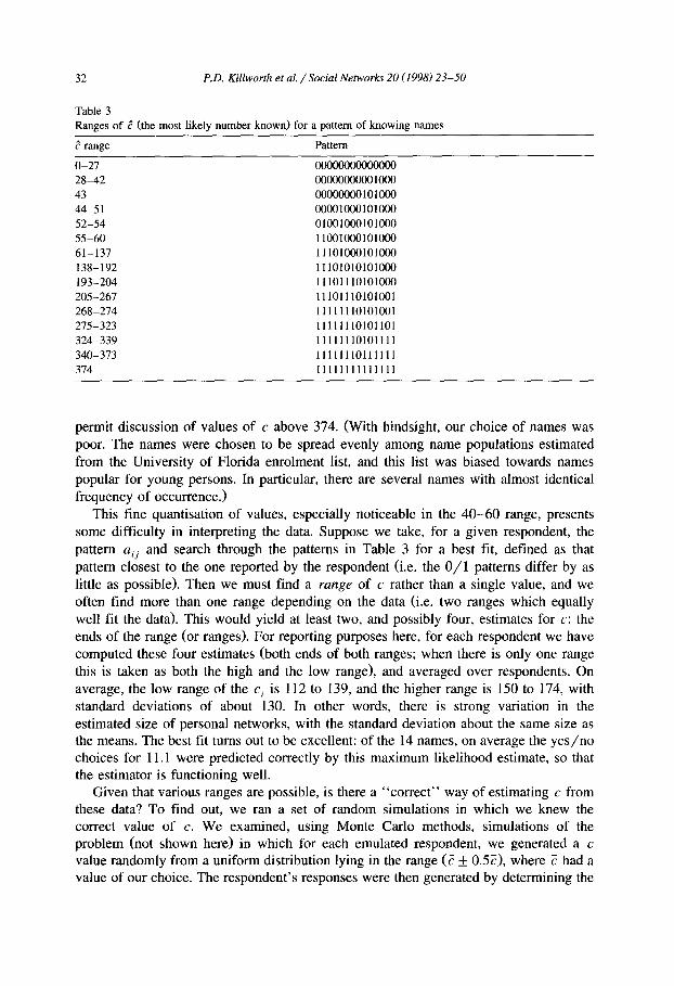
For c i < ~j, it is most likely that i does n o t know someone with name j; for c i > ~j, it is most likely that i d o e s know someone with name j. Note that these cutoff values are entirely generated by our choice of names. They divide the possible values for c i into regions, each region being bounded by one of the c j, or zero or t. The regions are shown in Table 3, together with the predicted patterns of y e s / n o answers for the 14 names. To distinguish between c values other than those shown requires more names: these must be extremely common to permit discussion of values of c less than 27, and rare to


Table 3 Ranges of d (the most likely number known) for a pattern of knowing names

range Pattern

0 -27 00000000000000 28-42 00000000001000 43 00000000101000 44-51 00001000101000 52-54 01001000101000 55-60 11001000101000 61-137 11101000101000 138-192 11101010101000 193-204 11101110101000 205-267 11101110101001 268-274 11111110101001 275-323 11111110101101 324-339 11111110101111 340-373 11111110111111 374 11111111111111

permit discussion of values of c above 374. (With hindsight, our choice of names was poor. The names were chosen to be spread evenly among name populations estimated from the University of Florida enrolment list, and this list was biased towards names popular for young persons. In particular, there are several names with almost identical frequency of occurrence.)

This fine quantisation of values, especially noticeable in the 40-60 range, presents some difficulty in interpreting the data. Suppose we take, for a given respondent, the p a t t e r n ai j and search through the patterns in Table 3 for a best fit, defined as that pattern closest to the one reported by the respondent (i.e. the 0 / 1 patterns differ by as little as possible). Then we must find a r a n g e of c rather than a single value, and we often find more than one range depending on the data (i.e. two ranges which equally well fit the data). This would yield at least two, and possibly four, estimates for c: the ends of the range (or ranges). For reporting purposes here, for each respondent we have computed these four estimates (both ends of both ranges; when there is only one range this is taken as both the high and the low range), and averaged over respondents. On average, the low range of the c i is 112 to 139, and the higher range is 150 to 174, with standard deviations of about 130. In other words, there is strong variation in the estimated size of personal networks, with the standard deviation about the same size as the means. The best fit turns out to be excellent: of the 14 names, on average the yes /no choices for 11.1 were predicted correctly by this maximum likelihood estimate, so that the estimator is functioning well.

Given that various ranges are possible, is there a "correct" way of estimating c from these data? To find out, we ran a set of random simulations in which we knew the correct value of c. We examined, using Monte Carlo methods, simulations of the problem (not shown here) in which for each emulated respondent, we generated a c value randomly from a uniform distribution lying in the range (? ___ 0.57), where ? had a value of our choice. The respondent's responses were then generated by determining the


pj for each name and choosing to emulate the respondent's knowing or not knowing a name based on a random number generated between 0 and 1 ; if it was less than pj then the name was known. (In other words, we emulated precisely what our model would prescribe.) We find, providing ? is well determined by our choice of names (i.e. lies between 0 and, say, 200 here), that the low end of the lower range reproduces accurately; the other ends of the ranges yield significant overestimates. Henceforth we choose to work with the lower end of the lower estimate, 113, for definiteness. Because we seek active networks in this study, we anticipate the value of ? being much smaller than the 1700 + 400 figure applicable to the global network.

Fig. 1 shows the histogram of c values computed in this manner. Note that " > 350" must here be interpreted as " 3 7 4 " since this also is the only available value given our choice of names. The shape of this histogram, unlike others presented later in this paper, differs from those found using telephone book methods (Freeman and Thompson, 1989; Killworth et al., 1990), although the sizes are much larger for these global networks.

If each estimate c i is then used in Eq. (1) to estimate the size e for the seropositive subpopulation, and these are averaged over all respondents, we obtain a value for e of 1.9 million, s.d. 6.6 million, standard error of the mean 0.2 million (the median is zero: more than half the respondents knew of nobody HIV-positive). One would prefer, for any estimate of e, that the standard deviation of the estimate be small. This cannot be the case for two reasons. First, estimates are probabilistic and so must vary. Second, the situation is made worse because our maximum likelihood estimate is quantised by the 14 y e s / n o decisions.

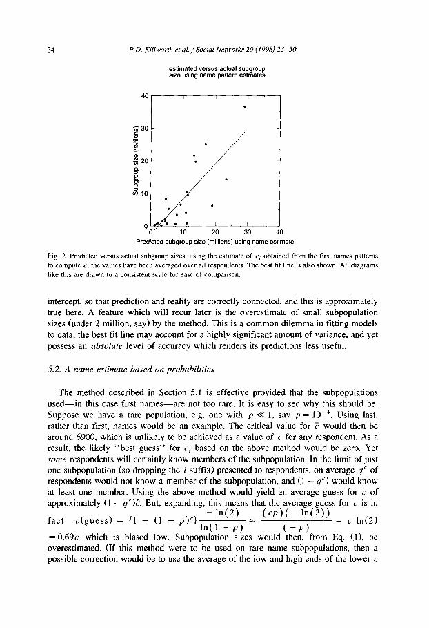
A measure of the reliance we may place on this estimate can be obtained by estimating the e for the other subpopulations, using the value of c i found for each respondent, and the formula in Eq. (1), in the same manner as for the seropositive subpopulation. Fig. 2 shows the results, plotted against actual subpopulation sizes. The correlation between predicted and observed is 0.82, and the best fit line has a slope of 1.01, and an intercept of - 2 . 5 million. The slope should, ideally, be unity, with a zero

histogram of c values using estimate based on name patterns

4OO r (D

"O ~- 300- 0 CL

"6 d

0 0-49 50-99 100-149 150-199 200-249 250-299 300-349 >350

Distribution of c values

Fig. 1. Histogram of c estimates using the name pattern method.

34 P,D. Killworth et aL / Social Networks 20 (1998) 23-50

estimated versus actual subgroup size using name pattern estmates

40 f f i

30

•

~ • ~ 2 0 •

-

m l O

• me• ii 0

Predicted subgroup size (millions) using name estimate

Fig. 2. Predicted versus actual subgroup sizes, using the estimate of c i obtained from the first names patterns to compute e; the values have been averaged over all respondents. The best fit line is also shown. All diagrams like this are drawn to a consistent scale for ease of comparison.

intercept, so that prediction and reality are correctly connected, and this is approximately true here. A feature which will recur later is the overestimate of small subpopulation sizes (under 2 million, say) by the method. This is a common dilemma in fitting models to data; the best fit line may account for a highly significant amount of variance, and yet possess an absolute level of accuracy which renders its predictions less useful.

5.2. A name estimate based on probabilities

The method described in Section 5.1 is effective provided that the subpopulations used - - in this case first names- -a re not too rare. It is easy to see why this should be. Suppose we have a rare population, e.g. one with p << l, say p = 10 - 4 . Using last, rather than first, names would be an example. The critical value for ? would then be around 6900, which is unlikely to be achieved as a value of c for any respondent. As a result, the likely "bes t guess" for c i based on the above method would be zero. Yet some respondents will certainly know members of the subpopulation. In the limit of just one subpopulation (so dropping the i suffix) presented to respondents, on average q ' of respondents would not know a member of the subpopulation, and (1 - q") would know at least one member. Using the above method would yield an average guess for c of approximately (1 - qC)d. But, expanding, this means that the average guess for c is in

- l n ( 2 ) ( c p ) ( - l n ( 2 ) ) fac t c ( g u e s s ) = {1 - (1 - p ) ~ ' } = = c ln(2)

l n ( 1 - p ) ( - p ) = 0.69c which is biased low. Subpopulation sizes would then, t¥om Eq. (1), be overestimated. (If this method were to be used on rare name subpopulations, then a possible correction would be to use the average of the low and high ends of the lower c


h i s t o g r a m of c v a l u e s us ing m a x i m u m l i ke l i hood e s t i m a t e b a s e d on n a m e s

'~ 15o

o- 49 50- 99 100-149 150-1~9 200-249 250-299 300-349 350-399 400-449 450-499 >500

Distribution of c v a l u e s

Fig. 3. Histogram of c estimates using the maximum likelihood name method.

range, rather than just the lower. For the common names used here, such a method overestimates c by at least 50%, as would replacing the estimated c i by c i / l n ( 2 ) . )

It should not be assumed that the estimate is always biased. If p is not small (the case here), then the estimate for c; from the method can be above or below the true value. However, it would be useful to produce a method which is less quantised. The idea is to seek the value of c i which maximises the probability of the responses given.

This probability, for any c;, is, from Eq. (7),

P , ; = 1--I q~' I - I ( 1 - q S ' ) . (9) j:aij= 0 j:aij= l

In Appendix A we show that there is a unique value of c i for which this probability is largest. This value is then the maximum likelihood estimate for c; in the usual statistical sense, based on names (or any other 0 / 1 data). We also show that the value of c; is infinite if the respondent reports knowing at least one alter with each name, a possibility which did not occur in our data. This awkwardness prevents any estimate of bias, and in general it follows that there must be some. The results below suggest that this is the case.

Using this method, we find that the maximum likelihood estimate for c, averaged over all respondents, is 105 (s.d. 92), which is somewhat lower than the previous estimate. The mean probability for this is 0.036. Fig. 3 shows a histogram of the variation of network size. Given the quantisation in Fig. 1, the histograms are not dissimilar.

Back-estimating e for each informant for the seropositive subpopulation gives an average e = 2.8 million (s.d. 17 million, standard error of the mean 0.53 million). Not only is this estimate high by any standards, the standard deviation is large compared with the previous value. Because this and other subpopulation values do appear high, the comparison between estimated and observed sizes is not shown here.

5.3. A s u b g r o u p e s t ima te b a s e d on p r o b a b i l i t i e s

A similar technique to that described in Section 5.2 can be used to create an estimate of c i based on the known subgroup sizes. We assume that respondent i reports knowing


mij members of subpopulation j, j = 1,2 . . . . . L, where L = 7 in our case; the eighth subpopulation (seropositive) is the one we wish to estimate, by first obtaining the maximum likelihood estimate for c i. We assume that the probability of knowing any member of one subpopulation is independent from that for another subpopulation. Then, using the Pc notation again,

L P r o b ( i k n o w s m i j , J 1,2, , L ) = P c = . I - ~ . . . . . . -m,j "= . . . , q C,% P) '~qj (10)

j--l--

by the binomial theorem, where nC,, is the binomial coefficient. Here pj is taken to represent the proportion of subpopulation j in T, i.e. pj = e J t , where e i is the size of the jth subpopulation; qj is again 1 -P i" Appendix A again shows that there is a unique value of cg which maximises the probability in Eq. (10), and thus provides the maximum likelihood estimate. In other words our estimate ~i for c~ is

Ci = Ci such that Pc, is maximal.

In Appendix B, we discuss the possible bias of estimates of c, 1/c, and back-estimates of subpopulation size using this maximum likelihood estimate. We find that the estimate c given by Eq. (10) is unbiased. The standard error of the estimate is given by

= . / s . d . ( ~ i ) V E j ej

where the sum is taken over the known subpopulations. For any given respondent, t and ci are of course fixed. To reduce the standard error of the estimate it is necessary to increase the total size of all the known subpopulations.

Appendix B also shows that for small numbers of predictive subgroups (under 20, say), estimates of l / c and back-estimated subpopulation size are biased, except, coincidentally, for around six or seven predictive subgroups (the number used here). However, in future work it is clear that many more predictive subgroups should be used to remove the bias in the estimates.

Averaging over all respondents, the maximum likelihood estimate of Eq. (10) gives a mean network size of 105, s.d. 89. (The standard deviation for each individual estimate of c~ vanes depending on which set of subpopulations was presented, but on average would be 28 (using a value for c~ equal to the mean actually found)). Thus the observed spread of c~ values is larger than the estimated error in any given value.

The mean value of the predicted c i is encouragingly similar to the 113 obtained by using names (and using an independent calculation), and is not significantly different from it. The average probability, per respondent, that the respondent's reported mij values would be observed randomly with a network size having the predicted value for c i is 0.046, which we believe is high. This is, after all, a product of seven probabilities, all of reasonably rare events. (This can be quantified: as long as mgj is small, the binomial can be approximated by the Poisson distribution. The largest probability for an expected value of m is actually for m observations, and is e - m m m / m ! , which takes the values 1, 0.37, 0.27, 0.22 for m = 0,1,2,3 respectively. So a respondent who reports knowing one alter in only three subgroups, and none in the others, would only have an a

P.D. Killworth et aL / Social Networks 20 (1998) 23-50 37

histogram of c values using maximum likelihood estimate based on subgroups

5OO

O3 400 t -

t - O 3OO tD..

(1)

"+6 200

6 Z

100

0 0-49 50-99 100-149 150-199 200-249 250-299 300-349 >349


Fig. 4. Histogram of c estimates using a maximum likelihood method based on subgroup sizes.

priori probability of 0 . 3 7 3 = 0.051. This crudely demonstrates how well the observed mij have been fitted.)

Fig. 4 shows the histogram of the c estimates using this method. Note that the distribution is rather smoother than that for the quantised name estimate, but very similar to that for the maximum likelihood name estimate.

Back-substituting once more into Eq. (1), for each respondent, to estimate the size of the seropositive subpopulation, gives a mean size of 1.5 million, s.d. 3.8 million, standard error of the mean 0.1 million. This is once more of a similar size to that estimated using names. It is interesting that although the mean c is smaller than for the method in Section 5.1, so is the estimate of e, which is a little counterintuitive; examination of plots of c versus e are not enlightening.

histogram of c values using maximum likelihood estimates based on name-subgroup combination

"5

0-49 50-99 100-149150-199200-249250-299300-349350-399400-449450-499500-549


Fig. 5. Histogram of c estimates using the maximum likelihood estimate involving both names and subgroups.

38 P.D. Killworth et al. / Social Nem,orks 20 (1998) 23-50

estimated versus actual subgroup size using combined maximum likelihood estimates

40

~" 30

= -g N • ~ 20

O

m l 0

I I I

el ° • •

el • I , I , - -

/ 10 20 30 40

Predicted subgroup size (millions) using combined maximum likelihood estimate

Fig. 6. P red ic ted ve r sus actual subg roup sizes, us ing the m a x i m u m l ike l ihood es t ima te based on both n a m e s

and subgroups , for ind iv idua l n e t w o r k size c i, a v e r a g e d o v e r all r e l evan t respondents .

5.4. A combined estimate

In Section 5.2 and Section 5.3 above we sought c values to max•raise a probability. Precisely the same concept can be applied to max•raise the probability of observing both the names and the subgroup sizes simultaneously. This is straightforward computation- ally since both methods employ a recursively defined ~b(c), and these need merely to be multiplied. This calculation yields an average value of c of 97, s.d. 73 (again, none of these estimates are statistically different). Fig. 5 shows the histogram of c values for this calculation; once more it is similar to the others, and-- in shape--to those found by Freeman and Thompson (1989) and Killworth et al. (1990). Surprisingly for such a complex matching operation--2l separate probabilities are multiplied together--the mean probability is still 1.3%.

Back-estimates of the seropositive subpopulation size give 1.1 million, s.d. 4.9 million (which is the smallest standard deviation for the estimates presented here), and standard error of the mean 0.2 million. Fig. 6 shows the comparison between predicted and observed subgroup sizes. Here the correlation is 0.82, but the best fit line has a slope of 1.9 rather than unity.

5.5. Proportional estimates

There are simpler, though not necessarily more accurate, ways to estimate both network size and the size of the seropositive subpopulation. For each respondent we are given s e v e n mij values. From these we can compute a combined estimate for c, namely

~ L I mi j Ci c = I L (11)

' ~ ' j = 1 ej


which treats each of the seven subpopulations equally, and so should be a fairly robust estimate of c. Somewhat surprisingly, it is possible to show that for small values of m i : / c and pj, the estimate ci, c is almost the same as the maximum likelihood estimate (the proof is straightforward and not given here). Thus subject to trivial differences relating to averaging, missing data, etc., Eq. (11) should and does give a similar answer to Eq. (10). By Appendix B, it yields an unbiased estimate of c, and a known standard error, while estimates of 1 / c and back-estimated subpopulation sizes are biased unless at least 20 predictive subpopulations are used, or apparently the six we employed here.

It is also possible to take the seven individual estimates for c i, namely m i / / e i , which can then be averaged to give an estimate

t I

mij (12) Ci,a -7

L j= 1 ej

By similar methods to Appendix B, one can show that the estimate ci, . is unbiased, but the variance of the estimate is (tci/L2)y':f= l (1 /e : ) . Thus when one or more of the subpopulations are small, as is the case here, the estimate has an unacceptably high variance (we estimate a standard error of around 60-70) and cannot be expected to produce reliable answers; we include it for completeness.

This is borne out by the results. The average value of network size is found to be 117 (s.d. 117) for the estimate ci, c, and 399 (s.d. 594) for the estimate ci, a. Thus the ci, . estimate is well in line with the previous estimates--in particular Eq. (10), as predicted - - b u t the estimate ci, a achieves a distinctly higher value. This is less evident in the seropositive estimate, which averages 1.8 million (s.d. 7 million, standard error 0.2 million) for the c~,,. estimate, and 1.1 million (s.d. 18 million, standard error 0.5 million) for the c~., estimate. Because of the similarity between c~,,. and Eq. (10), the results are not shown.

5.6. Overal l est imate

The six estimates produced here for the average network size c (based on mutual recognition by sight or name, can be contacted, and have had contact within the last two years, in person, by phone or by mail) are thus: 113, 105, 105, 97, 117, and 399. Corresponding estimates for the size of the seropositive subpopulation are, respectively: 1.9, 2.8, 1.5, 1.1, 1.8, and 1.1 million. The extreme values obtained from the c a estimate confirm the theoretical result of a large variance. The high e for the second estimate suggests the same may be true in that case. The other four suggest a best guess for the sizes of c and e respectively of 108 and 1.6 million. Standard errors of the mean are of order 4 (for c) and 0.2 million (for e). Note that the latter figures are rather less than the variation between estimates.

6. Results averaging over respondents

The second way we may estimate c and hence subpopulation sizes is to perform the averaging over respondents before computing c. In previous studies with one subpopulation, effectively only this method could be used. The effects of this pre-averaging are unclear, since back-estimates for unknown subpopulations involve division by the


estimation averaging over all respondents

40 f ~ i

~'= 30

N "~ 201 • "

o

o~I0 . I-

0 / 2 4 6

Average number known in subgroup

Fig. 7. Size of subpopulatiens versus the average number of members of the subpopulation known to a respondent. The best fit line is shown. Also shown, dashed, is the fit from the average over all 14 names.

estimate for the mean of the c i (however obtained) and this is not a linear operation. Simple distributions of c give adequate results when pre-averaging occurs (Bernard et al., 1989), but more complicated ones may not - - the distributions we have illustrated from the previous methods have medians noticeably different from means, for example.

Fig. 7 shows the dependence of subpopulation size e~ on Mj, where

1 Rj

M j = ~j i~=lmij (13)

is the average number of members of subpopulation j reported by the Rj relevant respondents (column 3 in Table 1). If our simple theory were correct, and if averaging over all respondents produces no bias, then Fig. 7 should show a straight line. The scatter is encouragingly small (the correlation is 0.83), showing that our theory holds well. However, the scatter is numerically large--as are our other est imates-- i f one seeks to estimate the seropositive subpopulation size. Indeed, the best fit line predicts a negative subpopulation size for the seropositive subpopulation, where from Table 1, MH~ v = 0.63. A less optimal fit, defined to pass through the origin, is similar. It implies a mean c of about 80, which is somewhat smaller than our previous estimates. Using this value for c in Eq. (1) to estimate the size of the seropositive subpopulation yields a value of 1.3 million, roughly in line with previous estimates. However, Fig. 7 shows that small subgroup sizes (those under about 2 million, or with M r less than unity) are clearly overestimated by this method. One would prefer a value of c rather larger to achieve a good fit for these subpopulations. There are also hints that an exponential curve would fit better than the straight line predicted by theory.

A similar calculation can be made using average values of c computed from the names. This uses Eq. (3), together with the known proportions of name occurrences. As


an experiment, several different methods were used to compute c. A direct average over the 14 names yielded 112, s.d. 61, which is not significantly different from the estimates of the previous section; it yields the prediction shown by the dashed line in Fig. 7. Using Eq. (1), this implies a value for the HIV-positive subpopulation size of 1.3 million.

7. Discussion

This paper has examined both network sizes and estimates of the unknown size of a subpopulation, here those who are seropositive, by using scaling methods based on respondents' reports about subpopulations of k n o w n size. The method is both inexpen- sive (a typical survey costs around $6 per respondent) and fast (taking about one month - -other surveys were being conducted by the field service during the time of our survey) compared, we suspect, with traditional methods used by public health workers.

The maximum likelihood methods, which are unbiased for sufficiently many predictive subpopulations (the number six used here is coincidentally relatively unbiased, at least for the Monte Carlo tests in Appendix B), compute a best-guess network size for each respondent, back-estimate the seropositive subpopulation estimate, and then take averages of both, appear to yield consistent estimates of around 108 and 1.6 million respectively. We propose terming the use of Eq. (10), or, equivalently, Eq. (11), to estimate c i for each respondent, together with a method for back-estimating a subpopulation size e (here obtained by simple averaging of individual estimates of e using Eq. (1)) as a "network scale-up method". The later methods introduced, which averaged the data across all respondents be fore making any estimates, gave bipolar results: straight line fits to the theory using averaged data imply rather smaller average network sizes, of order 60, and rather high estimates for the seropositive subpopulation, of order 2.5 million, while simultaneously graphs of the data imply much s m a l l e r estimates for seropositive numbers (perhaps 0.5 million) and correspondingly larger estimates for network size.

Several things stand out from our results. • First names should be treated as any other definition of a subpopulation in future

studies, i.e. respondents should report how many people they know with a given name, not simply whether they know someone; this will remove the quantisation difficulties.

• Although all our fits were significant, the direct predictions produced either under- or overestimates of actual subpopulation size; this situation should be alleviated by the addition of more subpopulations, which reduces the standard error of the c estimate as shown in Appendix B.

• When tested by applying the methods to estimate the size of a subpopulation which is in fact of known size (i.e. by using all other subgroups to estimate the c i, and then back-estimating for the remaining subpopulation), the methods appear to overestimate small (known) subpopulation sizes, and this fact should be borne in mind in considering our estimate.

We now consider three other aspects of our results in more detail.


7.1. The size o f our estimate

Lacking detailed knowledge of the distribution of personal network sizes, we cannot make absolute pronouncements, subject to the above caveats. However, we can compare our figure with other estimates.

Between 1990 and 1993, approximately 6000 people tested seropositive in Florida, and probably around 50,000 during the entire HIV testing era up to 1990 when this estimate was made. Scaled up nationally by population (Florida contains 5% of the U.S. population), this gives 1 million in the seropositive subpopulation as of that date. However, estimates suggest that Florida residents account for 12% of AIDS cases; if HIV numbers vary locally as do AIDS numbers, using the 12% figure would give only about 420,000.

Public health officials, as we have seen, use a combination of the back-calculation method and a composite of the cohort studies to estimate seroprevalence on both a national and a state level. These methods may have large errors. As mentioned earlier, the use of AIDS ratios as a proxy for seroprevalence ratios may have some problems. For example, seropositive persons do not always seek medical assistance immediately upon contracting symptoms classifying them as having AIDS. Potential seropositive victims may frequently be tested at several hospitals; others may not have been tested for many reasons.

Although most seropositive persons with CD4 counts low enough to be classified as having AIDS under the modern definition will have developed opportunistic symptoms, there are clearly cases to the contrary, which leads to an underestimate of an unknown size. Finally, accurate census data for the scaling arguments are not always available, especially in inter-census years. Recent reports of undercounts in the 1990 census for particular groups (homeless, lower socioeconomic status, etc.) makes the scaling arguments based on social strata suspect. The cohort studies suffer from obvious biases.

The fact remains that our estimates are clearly high compared with CDC estimates of seroprevalence. The current estimate is 1 million, probably to be lowered to 0.8 million; and this estimate is for all those who are seropositive. In contrast, our estimate applies (presumably) mainly to those who have tested positive for HIV. Current estimates - - though suffering from the difficulties discussed--are that 417,000 have tested positive for HIV between 1990 and 1993. Our estimate of 1.6 million remains almost four times that figure.

7.2. The accuracy o f our estimate

As noted earlier, there is a difficulty factor associated with a respondent being aware of h is /her knowledge that someone is in a particular subpopulation. For example, it is very easy to be aware that one knows someone whose name is Michael if one does know a Michael. It is distinctly harder to be aware that one knows someone who is a twin (if one does know a twin), since news about twins does not appear to travel efficiently other than at the time of the twins' birth and within the subnetwork of female relatives; our earlier work (Shelley et al., 1990; Johnsen et al., 1995) seems to bear this out. Thus respondents' estimates of m for difficult-to-know subpopulations are almost


certainly underestimates of reality. In addition, it may be hard for respondents to estimate how many they know in larger populations (e.g. those who play golD, so that respondents may either under- or overestimate their answers.

How would misreporting affect the answers? First, imagine that all reporting of subgroup knowledge was consistently under-reported by some uniform factor y (a "difficulty" factor), so that any reported knowledge m was actually m' = ycp , where p is again the actual proportion of that subgroup in the population (in other words, e = tp as before). This would induce an estimate of c as c' = m ' / p = yc , which is less than c. Similar arguments apply, with high accuracy, for the more subtle estimates of this paper. However, if this estimate of c is now used to back-estimate another subpopulation (also under-reported by the same factor) we obtain e' = e, i.e. the correct answer.

However, suppose now that the target population--seropositive in this case-- is more seriously under-reported, by a different amount y ' < y from the other subpopulations. Then the estimate of its subpopulation size will be e' -= ( y ' / y ) e . In the case in which the subpopulations are all approximately correctly reported except for the target one, e' < e and the subpopulation size would be underestimated. Thus if we assume consistent under-reporting, our estimates remain correct; if the under-reporting varies with subpopulation, such that the target subpopulation is hard to know while other subpopulations are relatively easy--which is almost certainly the case for sensitive information such as seroprevalence--our estimates should be biased too low.

Unfortunately, we do not know how hard it is to know about subpopulations. There is little indication from our data that simply asking respondents to estimate the degree of difficulty involved with knowing about a subpopulation produces useful answers (the reader may try this: is it more difficult to know whether someone bought a house last year or is a twin?). This is confirmed by direct methods by Shelley et al. (1995). Instead, we need to induce the estimates of difficulty by seeking accurate data on a wider variety of subpopulations (and backed up with ethnographic detail). Some of these should be extremely easy to know about: our work (Johnsen et al., 1995) suggests that news concerning homicide victims travels very efficiently, for example. We imagine that information about deaths in highway accidents in a given year - - for which an accurate number is available--would travel equally efficiently (be equally easy to know). Armed with a collection of such subpopulations, we can seek estimates per respondent of h is /her network size. If these are consistent--and this remains to be shown--then we can add in other, harder-to-know-about, subpopulations and obtain the y factor for these post facto.

This approach yields results only when we have a known subpopulation size for comparison. When the subpopulation is of unknown size no y factors can be induced. Instead, we must probably be content with producing an underestimate of the subpopulation size, together with seeking ethnographic and other data to examine how information about people is passed between people.

7.3. Other factors affecting the accuracy o f the estimates

While this method of estimating seroprevalence is free of many of the biases associated with the methods reviewed above, there are several potential biases which are

44 P.D. Killworth et al. // Social Networks 20 (1998) 23-50

particular to this method, and which may serve to explain the high estimate of seroprevalence in the U.S. First, like all surveys which depend on immediate recall, there may be errors of memory. It may be unreasonable to expect respondents to be able to know, offhand, how many people they know who are seropositive. And since the estimate is also based on recall of ties to other subpopulations (e.g. diabetics, golfers or parents of twins), errors of recall may occur with these groups as well.

It is also likely that these estimates are subject to errors of cognition. Despite the rather lengthy definition of "knowing" , respondents may vary in their interpretation of what knowing means. More likely is variance in the interpretation of what constitutes seropositivity or AIDS. Given different levels of knowledge and experience with HIV, some respondents are no doubt more expert than others. Thus, some respondents may think an acquaintance is seropositive when in fact they are not; or less likely the reverse. This may not always be an error. Homosexuals may assume an acquaintance is seropositive given past behaviours when the acquaintance has actually never been tested. Thus, the high estimate of 1.6 million who know they are seropositive may actually include some who do not know it or who suspect it but have never been tested.

Related to this is the error of imperfect knowledge about their alters due to differential rates of information transmission concerning HIV status. Not only might some respondents have this information withheld from them by acquaintances who are seropositive, but the rate of transmission may be related to other sociodemographic characteristics such as age, gender, race or education. For instance, our ethnographic component revealed that black seropositive respondents were reluctant to tell other blacks their status for fear of shunning or other more serious reprisals (Shelley et al., 1995). Uneven information transmission may also occur with regard to a person's status within other subpopulations as well, such as American Indians or owning a swimming pool.

Ethnographic studies (Shelley et al., 1995) of the seropositive community in Atlanta pose other questions of our inferences. For example, the closer-knit structure with the seropositive community could lead to respondents tending to know the s a m e seroposi- five persons rather than a random sample of the population as a whole. This would probably induce an overestimate of the size of the seropositive subpopulation. The study also showed that some respondents claimed to know alters were seropositive because they showed the relevant symptoms, whether or not those alters had actually been tested positive. This possibility cuts both ways: on the one hand it could bias our estimates upwards, but on the other hand it could indicate omissions in national estimates.

Perhaps the greatest potential error arises from the restriction of the sample to Floridians. While the acquaintance pool of the respondents was not limited to Florida, the sample of respondents was. From survey data by McCarty (1997) we know that of the seropositive acquaintances known by Floridians, the majority of them are also Floridians. This follows from the fact that locality plays a large part in who you know (although 30% of our respondents' acquaintances were from outside Florida). Further, as noted above, we know that Florida has a higher incidence of AIDS (12%) and probably HIV than most states (5%). Thus, the pool of acquaintances of Floridians is more predisposed to be seropositive than are acquaintances in, say, West Virginia. At the same time, though, there is a weak but significant negative correlation between how


many of a respondent's alters lived outside Florida and how many seropositives the respondent knew. While our estimates are necessarily national, we very likely err on the high side given our respondent pool. (Put mathematically, the 3" value may be higher than 3' values, leading to an overestimate.) However, Florida may also have more than its proportional share of some of the other subgroups we chose (owners of swimming pools, etc.) which may reduce the error accordingly.

If Florida respondents only knew other residents of Florida, then the estimate of 1.6 million would have to be scaled down by 5%/12% = 42%, giving 0.67 million, close to official estimates. In fact, as noted above, 70% of Florida respondents' alters lived within Florida, which would modify the estimate further to 70% × 0.67 + 30% × (1.6 × ( 1 0 0 - 5 ) / ( 1 0 0 - 12))= 0.99 million; here the latter correction adjusts the value for alters outside Florida. Of course, features other than location could also be acting which would further such estimates.

It is important to discover if at least the possibility of local versus national reporting can occur. Accordingly, a repeat of this study on a national level has been completed: the results will be reported and compared elsewhere.

Note added in proof

Examination of source data for references has yielded estimates for some subpopulation sizes which differ by up to 60% from those used in this paper, e.g. for some sports. We cannot determine which estimates are more reliable. Readers should thus be aware that values for c and subpopulation sizes depend on the values chosen for source data, so that the values cited here may be subject to some degree of error, depending upon which set of source data are chosen.

Acknowledgements

This work was conducted under NSF grant #SBR-9213615. Much of the analysis took place with the welcome hospitality of the Bureau of Economic and Business Research at the University of Florida, who also provided computing support. Ed Laumann provided a useful critique of a draft of this paper,

Appendix A. Notes on maximum likelihood estimates

A. 1. The name est imate (Eq. (P))

Consider the process of changing c i until P,,, is maximal. We note that (a) P0 = 0; (b) Pc ~ 0, c ~ ~; (c) Pc -> 0. Further,

P~+l 1-i qj i--i ( l _-_qj~_~ +' ) 6 ( c ) Pc j:,,j= 0 j : , , j=, 1 - q ~

is clearly less than unity for large c (unless the respondent reports knowing at least one alter with each name, so that the first product is unity; we shall consider this possibility

46 P.D. Killworth et al. / Social Networks" 20 (1998) 23-50

below). Also, the first product does not depend on c, and the second product decreases with c. (To see this, consider the inequality between the term for c and that for c + 1; the proof is straightforward.) Thus ~b(c) is either less than unity for c = 1 (so that c = 1 makes the probability largest), or ~b(c) becomes less than unity as c increases. Hence there is a unique value of ci for which P~i is maximal. Numerically this can be located by computing successive values of ~b(c) until it drops below unity.

However, this proof fails when the respondent knows at least one alter with each name, when clearly Pc increases with c asymptotically closer to unity. While this did not occur in our data, this possibility prevents any estimate of bias from being made; in general, this possibility means that the estimate must be biased.

A.2. The subgroup estimate (Eq. (10))

If c i is the most likely value for i 's network size in Eq. (10), we require

P~,> Pa, d~:ci. (A.I )

Now from Eq. (10), we have after a little simplification, for any value of c,

P~.+, = f i ( c + l ) q j (1 .2 ) Pc j = l ( C + l - m i j )

which must be less than unity if Eq. (1.1) is to hold. Now we can write Eq. (A.2) as

Pc+l I -IL j= lqj

P " - = ~b(c)= 1-ILj=I(1 c~-lmi j ) . (1 .3 )

In this form it is clear that: (a) ~b(c) is infinite when c + 1 is the largest of the mii; (b) ~b(c) decreases with c; and (c) for large c, ~b(c) is clearly less than 1. Thus there is again one unique value for c (which we take to be c i) for which Eq. (A. 1) holds. To find it, one merely increases c until ~b(c) is less than unity. The value of c i is then the maximum likelihood estimate for that respondent. (Two special cases demonstrate this. In the case of L = 1, this yields simply c ~- m/p , as in our original formula. If mij = cpj for all j, then c is also found correctly.) The estimate of c increases for larger mii, and can be thought of as a suitably weighted average of the mij /p j , since, from Eq. (A.3), c lies between the minimum and maximum of the miJpj . The actual probability P, can also be computed for that value of c i, using Eq. (10).

Appendix B. Sources of bias in subgroup estimates

We first discuss the estimate of c i given by Eq. (10), or, equivalently, but more conveniently, Eq. (11). Denoting the estimate by ~i again, we have that

~jmij 3 i = t ~jej

P.D. Killworth et al. / Social Networks 20 (1998) 2 3 - 5 0 47

and we note that the mij are c i random numbers drawn from a binomial distribution with probability p~ = e J t , and all the j are independent. Denoting expectancies by E, we have

t t c i t Y ~ j e J t _ e(ai) = w - - - F _ , E ( m i j ) = w - - • ( c i p j ) = c,

Eje~ L:e:2_.,j j j Z_,;e;j j j

so that the estimate is unbiased. Similarly, the variance of the estimate is given by

t t var(~i) = Y'~var(mij) ~- E c i e J t = - - c i

j j ~ j e j

provided that the fractional size of any subgroup e J r is small. Hence the standard error of the estimate is

t c i s.d.(Oi) = Ej ej

and normal confidence intervals would be expected to hold. However, although the estimates for c are unbiased, the same need not be true when

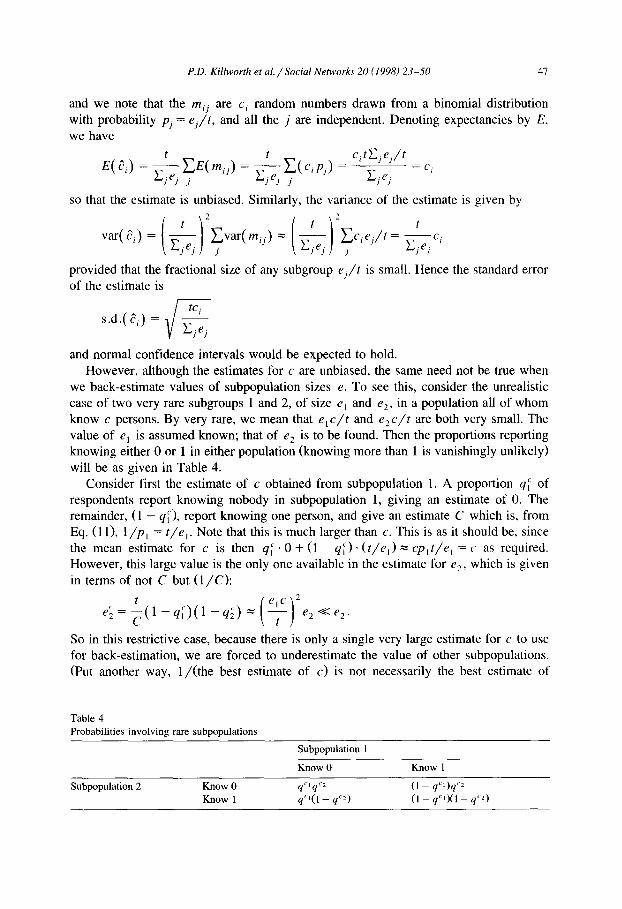
we back-estimate values of subpopulation sizes e. To see this, consider the unrealistic case of two very rare subgroups 1 and 2, of size e I and e 2, in a population all of whom know c persons. By very rare, we mean that e ~ c / t and e 2 c / t are both very small. The value of ej is assumed known; that of e 2 is to be found. Then the proportions reporting knowing either 0 or 1 in either population (knowing more than 1 is vanishingly unlikely) will be as given in Table 4.

Consider first the estimate of c obtained from subpopulation 1. A proportion qi: of respondents report knowing nobody in subpopulation 1, giving an estimate of 0. The remainder, (1 - q~), report knowing one person, and give an estimate C which is, from Eq. (11), l i p I = t / e j . Note that this is much larger than c. This is as it should be, since the mean estimate for c is then q~. 0 + (1 - q~) . ( t / e I) -~ c p l t / e I = c as required. However, this large value is the only one available in the estimate for e 2, which is given in terms of not C but ( l / C ) :

el= ~(1- q ~ ) ( 1 - q ; ) = e2<<e 2.

So in this restrictive case, because there is only a single very large estimate for c to use for back-estimation, we are forced to underestimate the value of other subpopulations. (Put another way, 1/ ( the best estimate of c) is not necessarily the best estimate of

Table 4 Probabilities involving rare subpopulations

Subpopul~ion l

Know 0 Know 1

Subpopulation 2 Know 0 q,'l qC2 (1 - qC~ )qC 2

Know 1 q,'l(1 _ qC2) (1 - q"O(1 - q"2)


( l / c ) , since averaging and divisions do not commute.) Other examples could produce the opposite effect, of overestimating subpopulation sizes.

Thus for reliability, we should seek for many subpopulations, which will alleviate the zero problems discussed above and, hopefully, remove the biases in estimates of 1/c.

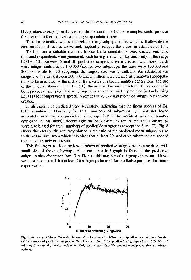
To find out a suitable number, Monte Carlo simulations were carried out. One thousand respondents were generated, each having a c which lay uniformly in the range (200 + 150). Between 2 and 30 predictive subgroups were created, with sizes which were integer multiples of 100,000 (i.e. for two subgroups, the sizes were 100,000 and 200,000, while for 30 subgroups the largest size was 3 million). An additional ten subgroups of sizes between 500,000 and 5 million were created as unknown subpopulations to be predicted by the method. By a series of random number generations, and use of the binomial theorem as in Eq. (10), the number known by each model respondent in both predictive and predicted subgroups was generated, and c predicted (actually using Eq. (11) for computational speed). Averages of c, 1 / c and predicted subgroup size were created.

In all cases c is predicted very accurately, indicating that the linear process of Eq. (11) is unbiased. However, for small numbers of subgroups 1/c was not found accurately save for six predictive subgroups (which by accident was the number employed in this study). Accordingly the back-estimates for the predicted subgroups were also biased for small numbers of predictiVe subgroups (except for 6 and 7!). Fig. 8 shows this clearly: the accuracy plotted is the ratio of the predicted mean subgroup size to the actual size, from which it is clear that at least 20 predictive subgroups are needed to achieve an unbiased result.

This finding is not because low numbers of predictive subgroups are associated with small size of those subgroups. An almost identical graph is found if the predictive subgroup size decreases from 3 million as thE number of subgroups increases. Hence we must recommend that at least 20 subgroups be used for predictive purposes for future experiments.

1.5 I i

o o

0 . 5

0 , I , I ,

0 1 0 20 30 Number of predicting subgroups

Fig. 8. Accuracy of Monte Carlo simulations of back-estimated subGroup size (predicted/actual) as a function of the number of predictive subgroups. Ten lines are plotted, for predicted subgroups of size 500,000 to 5 million; all essentially overlie each other. Only six, or more than 20, predictive subgroups give an unbiased estimate.

P.D. Killworth et al. / Social Networks" 20 (1998) 23-50 49

References

Altman, R., S.I. Shahled, W. Pizzuti, D.N. Brandon, L. Anderson and C. Freund, 1992, Premarital HIV-1 testing in New Jersey, Journal of Acquired Immune Deficiency Syndromes 5, 7-11.

Bernard, H.R., E.C. Johnsen, P.D. Killworth and S. Robinson, 1989, Estimating the size of an average personal network and of an event subpopulation, in: M. Kochen, ed., The small world (Ablex, Norwood, NJ) 159-175.

Bernard, H.R., E.C. Johnsen, P.D. Killworth, C. McCarty, S. Robinson and G.A. Shelley, 1990, Comparing four different methods for measuring personal social networks, Social Networks 12, 179-215.

Bernard, H.R., E.C. Johnsen, P.D. Killworth and S. Robinson, 1991, Estimating the size of an average personal network and of an event subpopulation: Some empirical results, Social Science Research 20, 109-121.

Brundage, J.F., D.S. Burke, LI. Gardner, J.G. McNeil, M. Goldenbaum, R. Visintine, R.R. Redfield, M. Peterson and R.N. Miller, 1990, Tracking the spread of HIV infection epidemic among young adults in the United States: Results of the first four years of screening among civilian applicants for U.S. military service, Journal of Acquired Immune Deficiency Syndromes 3, 1168-1180.

Centers for Disease Control (CDC), 1990, HIV prevalence estimates and AIDS case projections for the United States: Report based upon a workshop, Morbidity and Mortality Weekly Report 39, 7.

De Gruttola, V. and H.V. Fineberg, 1989, Estimating prevalence of HIV infection: Considerations in the design and analysis of a national seroprevalence survey, Journal of Acquired Immune Deficiency Syndromes 2, 472-480.

Freeman, L.C. and C.R. Thompson, 1989, Estimating acquaintanceship volume, in: M. Kochen, ed., The small world (Ablex, Norwood, NJ) 159-175.

Gail, M.H. and R. Brookmeyer, 1988, Methods for projecting course of acquired immune deficiency syndrome epidemic, Journal of the National Cancer Institute 80, 900-911.

Johnsen, E.C., H.R. Bernard, P.D. Killworth, G.A. Shelley and C. McCa~y, 1995, A social network approach to corroborating the number of AIDS/HIV + victims in the U.S., Social Networks 17, 167-187.

Johnsen et al., in preparation. Killworth, P.D., E.C. Johnsen, H.R. Bernard, G.A. Shelley and C. McCarty, 1990, Estimating the size of

personal networks, Social Networks 12, 289-312. Laumann, E.O., J.H. Gagnon, S. Michaels, R.T. Michael and L.P. Schumm, 1993, Monitoring AIDS and other

rare population events: A network approach, Journal of Health and Social Behavior 34, 7-22. McCarty, C., 1997, Subgroups in personal networks: The inside view. American Journal of Community

Psychology (submitted). McCarty, C., H.R. Bernard, P.D. Killworth, E~C. Johnsen and G.A. Shelley, 1997, Eliciting representative

samples of personal networks, Social Networks (in press). McQuillan, G.M,, M. Khare, T.M. Ezzat, C.A. Schable and R.S. Murphy, 1993, The seroepidemiology of

human immunodeficiency virus in the United States household population: NHANES III, 1988-1991, paper presented at the First National Conference on Human Retroviruses and Related Infections, Washing- ton, DC.

National Multiple Sclerosis Society, 1992, Memorandum No. 62-92, 4 March 1992. National Sporting Goods Association, 1992, Sports participation in 1992, Mr. Prospect, 16. Statistical

Resources Index 1993, A8485-3. NSP1 Market Research and Statistics Committee, 1991, National Spa and Pool Institute pool and spa market

study for the year 1990. Rosenberg, P.S., R. Biggar, J.J. Goedert and M.H, Gail, 1991, Backcalculation of the number with human

immunodeficiency virus infection in the United States, American Journal of Epidemiology 133, 276-285. Shelley, G.A., H.R. Bernard and P.D. Killworth, 1990, Information flow in social networks, Journal of

Quantitative Anthropology 2, 201-225. Shelley, G.A., H.R. Bernard, P.D. Killworth, E.C. Johnsen and C. McCarty, 1995, Who knows your HIV

status? What HIV+ patients and their network members know about each other, Social Networks 17, 189-217.

Statistical Abstracts of the United States, 1993, U.S. Dept. of Commerce, Economics and Statistics Adminis- tration, Bureau of the Census.


U.S. Civil Airmen Statistics, 1993, U.S. Dept. of Transportation, Federal Aviation Administration, Office of Management Systems, ASI 1993 7504-2, Annual report series, SRI 1993 A9415-1.

Vital and Health Statistics, 1992, "Health and Demographic Characteristics of Twin Births: United States, 1988", Center for Disease Control, National Center for Health Statistics, Hyattsville, Maryland, Series 21, number 50, U.S. Public Health Service.

A social network approach to estimating seroprevalence in...

Documents

Transcript of A social network approach to estimating seroprevalence in...