Discussion Paper No. 742

A SMALL FIRMS LEADS TO

CURIOUS OUTCOMES: SOCIAL SURPLUS, CONSUMER SURPLUS,

AND R&D ACTIVITIES

Toshihiro Matsumura and

Noriaki Matsushima

June 2009

The Institute of Social and Economic Research Osaka University

6-1 Mihogaoka, Ibaraki, Osaka 567-0047, Japan

A small firm leads to curious outcomes: Social surplus,consumer surplus, and R&D activities∗

Toshihiro Matsumura

Institute of Social Science, University of Tokyo

Noriaki Matsushima†

Institute of Social and Economic Research, Osaka University

June 3, 2009

Abstract

This paper investigates an asymmetric duopoly model with a Hotelling line. We

find that helping a small (minor) firm can reduce both social and consumer surplus.

This makes a sharp contrast to existing works showing that helping minor firms can

reduce social surplus but always improves consumer surplus. We also investigate R&D

competition. We find that a minor firm may engage in R&D more intensively than a

major firm in spite of economies of scale in R&D activities.

JEL classification: L13, O32, R32

Key words: product selection, minor firm, R&D

∗ The authors gratefully acknowledge financial support from Grant-in-Aid for Encouragement of Young

Scientists from the Japanese Ministry of Education, Science and Culture. Needless to say, we are responsible

for any remaining errors.† Corresponding author: Noriaki Matsushima, Institute of Social and Economic Research, Osaka Univer-

sity, Mihogaoka 6-1, Ibaraki, Osaka 567-0047, Japan. Phone: +81-6-6877-5111 (ex. 9170), Fax: +81-6-6878-

2766, E-mail: nmatsush@iser.osaka-u.ac.jp

1

1 Introduction

Common observation suggests that firms in the same industry often differ in their market

conduct and performance. Large and small firms tend to have different features in their

strategies. For instance, it has been believed that small (minor) firms should differentiate

their products from those of major firms because the minor firms do not have any advantage

over the major firms if they do not differentiate their products. Moreover, it is also widely

believed that major firms invest more in R&D. In other words, minor firms invest less in

R&D.1 After all, it is often considered that the market impact of small firms is not so large.

From the view of social welfare, however, it is unclear whether or not those strategic conducts

of small firms are beneficial. Therefore, investigating strategic behaviors of minor firms is

an important research topic in the literature of not only industrial organization but also

management strategy. Using a simple Hotelling model, we consider how a small firm affects

consumer and social surplus and R&D expenditures.

In their pioneering work, Lahiri and Ono (1988) investigate an asymmetric Cournot

duopoly and show that an increase in the cost of an inferior firm improves welfare when

the cost difference between firms are sufficiently large, that is, helping a minor firm reduces

welfare.2 An increase in the cost of the inferior firm reduces its output, and through the

strategic interaction between the firms, the output of the superior firm increases. This

production substitution economizes on total production costs and thus improves welfare.

This result implies that eliminating the inferior firm (minor firm) improves welfare. Wang and

Zhao (2007) show that in both Cournot and Bertrand models with product differentiation,

an increase in the cost of the inferior firm can improve welfare.

Although those studies of asymmetric oligopoly show that enhancing competition can1 As explained later, it is not always true. Cohen and Klepper (1996) mention counterexamples to this

statement.

2 Zhao (2001) provides a sufficient condition for the proposition. For the applications of this mechanism,

see Lahiri and Ono (1997, 1998). Salant and Shaffer (1999) also provide important welfare implications on

asymmetric Cournot models.

2

reduce welfare, enhancing competition improves consumer welfare in all the papers mentioned

above. In contrast to the existing works, we present a situation where helping a minor

firm reduces both social surplus and consumer surplus by incorporating product positions

of asymmetric firms. We show this by using an asymmetric location-price model with a

Hotelling line.3 We find that a decrease in the cost of the inferior firm distorts the product

selection by the superior firm and can reduce both consumer and social surplus.

We believe that investigating the relation between firm heterogeneity and social welfare in

a location model is an important issue because we can investigate several important points

within this framework. First, we can investigate how product varieties (the locations of

firms) in a market are endogenously determined. In other words, we can investigate which

firm produces a mainstream product (locates at a central point). Second, we can investigate

whether these equilibrium product varieties (the locations of firms) are efficient from the

viewpoint of social and consumer welfare. A typical example related to our motivation

is the optimal product positioning strategies of asymmetric firms in the context of retail

outlet locations in the fast food industry (see Thomadsen (2007)). In many cities, both

McDonald’s (the stronger competitor) and Burger King (the weaker competitor) seek optimal

locations. McDonald’s avoids moderate amounts of differentiation while Burger King tries to

differentiate itself, and Burger King is more likely than McDonald’s to choose a suboptimal

location (Thomadsen (2007)). In this case, investigating the efficiency of those location

strategies has the potential to provide an insight on policy for land use and regulation of

zoning.

We also investigate R&D competition between asymmetric firms. The larger the firm,

the greater is the output over which it can apply the fruits of its R&D and hence the greater

its returns from R&D (Cohen and Klepper, 1996). Thus, it is widely believed that major

firms invest more in R&D. In this paper, we show that the minor firm can have a stronger

3 For the equilibrium location under an asymmetric cost structure in the Hotelling model, see Ziss (1993),

Tyagi (2000), Liang and Mai (2006), and Matsumura and Matsushima (2009).

3

incentive for R&D. In our model, a decrease in the cost of the minor firm distorts the product

selection of the major firm. This strategic effect can dominate the economy of scale effect

mentioned above, and yields a counterintuitive result, that is, the minor firm can invest more

than the major firm. Although it is widely observed that firms with larger market shares

aggressively invest in R&D, it is also observed that minor firms are not always inactive and

those with small market share engage in outstanding R&D (Cohen and Klepper (1996) and

Rogers (2004)). Our result provides a new insight in the literature of the relation between

firm size and R&D.4

Innovation by Harley Davidson in 1980s may be a typical example in which a minor

firm can have a stronger incentive for R&D. Harley Davidson had only about a 5% share

in the US motorcycle market. In this sense, it was a minor firm. Significant innovation by

Harley Davidson has affected the product positioning of Japanese rivals such as Honda and

Kawasaki and resulted in great success for Harley Davidson (see Reid (1991) and Kitano

(2008)).5

Meza and Tombak (forthcoming) is closely related to our paper. They also discuss an

asymmetric location-price model with a Hotelling line. They discuss three main topics: (1)

endogenous timing of entries (locations), (2) mixed strategies of location, and (3) comparison

between the social optimum and the equilibrium locations. They do not deal with our two

main concerns: (1) the relation among cost difference, consumers and social welfare and (2)

4 Our discussion is quite different from the well-known Arrow effect: a potential entrant obtains greater

value from drastic innovation than an incumbent monopolist. In the Arrow (1962) setting, a potential

entrant and an incumbent monopolist have the same opportunity to achieve a drastic innovation to reduce

their production cost. Before the R&D investment, the incumbent monopolist is more efficient than the

potential entrant. In other words, the entrant’s additional gain from the drastic innovation is higher than

that of the incumbent monopolist although the investment cost is the same for both. By assumption, the

potential entrant has a better opportunity than the monopolist (see also Tirole (1988, Ch.10)). In our model,

however, the firms’ investment technologies are the same. That is, if the investment level of a minor firm is

equal to that of a major firm, the levels of their cost reductions are the same.

5 An older example of a small firm is Tokyo Telecommunications Engineering Corporation (forerunner of

SONY) in the Japanese radio market. It competed with Matsushita (forerunner of Panasonic) and Hayakawa

(forerunner of SHARP). A newer example of a small firm may be Mitsubishi Automobile in the Japanese

electric automobile market. It competes with Toyota and Honda.

4

R&D competition among asymmetric firms. Our paper and Meza and Tombak (forthcoming)

are complementary in the sense that one increases the value of the other.

The remainder of the paper is organized as follows. Section 2 presents the basic model.

Section 3 provides the result for consumers and social welfare. Section 4 discusses the levels

of R&D investment, and Section 5 concludes.

2 The model

Consider a linear city along the unit interval [0, 1], where firm 1 is located at x1 and firm 2

is located at 1− x2. Without loss of generality, we assume that x1 ≤ 1− x2. Consumers are

uniformly distributed along the interval. Each consumer buys exactly one unit of the good,

which can be produced by either firm 1 or 2. Let pi denote the price of firm i (i = 1, 2). The

utility of the consumer located at x is given by:

ux ={ −t(x1 − x)2 − p1 if bought from firm 1,−t(1− x2 − x)2 − p2 if bought from firm 2,

(1)

where t represents the exogenous parameter of the transport cost incurred by the consumer.

For a consumer living at x(p1, p2, x1, x2), where

−t(x1 − x(p1, p2, x1, x2))2 − p1 = −t(1− x2 − x(p1, p2, x1, x2))2 − p2, (2)

the utility is same whichever of the two firms is chosen. We can rewrite (2) as follows:

x(p1, p2, x1, x2) =1 + x1 − x2

2+

p2 − p1

2t(1− x1 − x2).

Thus, the demand facing firm 1, D1, and that facing firm 2, D2, are given by:

D1(p1, p2, x1, x2) = min{max(x(p1, p2, x1, x2), 0), 1},D2(p1, p2, x1, x2) = 1−D1(p1, p2, x1, x2).

(3)

We assume that one of the firms (denoted as firm 2) has a cost disadvantage. Assume

the marginal costs of both firms are c1 = c and c2 = c + d, where c is a positive constant

and d is the cost disadvantage of firm 2.

5

The profit functions of the firms are:

π1 = (p1 − c)D1(p1, p2, x1, x2), π2 = (p2 − (c + d))D2(p1, p2, x1, x2).

Consumer surplus and social welfare are written as

CS =∫ D1

0(v − p1 − t(x− x1)2)dx +

∫ 1

D1

(v − p2 − t(1− x2 − x)2)dx, (4)

SW =∫ D1

0(v − c− t(x− x1)2)dx +

∫ 1

D1

(v − (c + d)− t(1− x2 − x)2)dx. (5)

The game runs as follows. In the first stage, firm 1 chooses its location x1 ∈ [0, 1/2] (by

symmetry, x1 ≥ 1/2 is equivalent to 1− x1(≤ 1/2)). Observing the location of firm 1, firm

2 chooses its location x2 ∈ [0, 1]. In the second stage, firm i chooses its price pi ∈ [ci,∞)

simultaneously.

3 Result

In this section, we derive the equilibrium locations, profits, consumer surplus, and total

social surplus.

3.1 Locations and profits

First, we investigate a price competition stage. Given the locations of firms, x1 and x2, the

firms face Bertrand competition. Let the superscript ‘B’ denote the equilibrium outcome at

the price-competition stage given x1 and x2. The equilibrium prices are:

pB1 =

c + d− t(1− x1 − x2)(1− x1 + x2) if d ≥ t(1− x1 − x2)(3− x1 + x2),3c + d + t(1− x1 − x2)(3 + x1 − x2)

3if d < t(1− x1 − x2)(3− x1 + x2),

pB2 =

c + d if d ≥ t(1− x1 − x2)(3− x1 + x2),3c + 2d + t(1− x1 − x2)(3− x1 + x2)

3if d < t(1− x1 − x2)(3− x1 + x2).

If d ≥ t(1 − x1 − x2)(3 − x1 + x2), DB1 = 1 and D2 B = 0 (monopoly by firm 1 and firm 2

only serves as a potential competitor). If d < t(1−x1−x2)(3−x1 +x2), both firms produce

in the market (DB1 , DB

2 > 0).

6

The resulting profits of the firms are:

πB1 =

d− t(1− x1 − x2)(1− x1 + x2) if d ≥ t(1− x1 − x2)(3− x1 + x2),(d + t(1− x1 − x2)(3 + x1 − x2))2

18t(1− x1 − x2)if d < t(1− x1 − x2)(3− x1 + x2),

(6)

πB2 =

0 if d ≥ t(1− x1 − x2)(3− x1 + x2),(t(1− x1 − x2)(3− x1 + x2)− d)2

18t(1− x1 − x2)if d < t(1− x1 − x2)(3− x1 + x2).

(7)

Second, we consider the location choice of firm 2. Given the location of firm 1, x1, firm 2

decides its location.6 Lemma 1 states that the optimal location of firm 2 does not depend on

x1. Henceforth let the superscript‘*’ denote the subgame perfect Nash equilibrium outcome

in the full game.

Lemma 1 For any x1(≤ 1/2), the optimal location of firm 2 is 1 (i.e., x∗2 = 0).

As pointed out by d’Aspremont et al. (1979), to mitigate price competition, firm 2 maximizes

the degree of product differentiation given the location of firm 1.

Third, we consider the location choice of firm 1. We have the following lemma:

Lemma 2 (Meza and Tombak (forthcoming)) When the locations are sequentially deter-

mined, the optimal location of firm 1 is:

x∗1 =

0 if d ≤ t,

t−√

(4t− 3d)t3t

if t < d ≤ (29√

145− 187)t128

' 1.267t,

12

if(29√

145− 187)t128

≤ d.

(8)

6 Note that, if d > t(1− x1)(3− x1), it is indifferent what location is chosen by firm 2.

7

The resulting profits of the firms are:

π∗1 =

(3t + d)2

18tif d ≤ t,

8(4t + 3d + 2√

t(4t− 3d))2

243(2t +√

t(4t− 3d))if t < d ≤ (29

√145− 187)t128

' 1.267t,

d− t

4if

(29√

145− 187)t128

≤ d.

π∗2 =

(3t− d)2

18tif d ≤ t,

2(10t− 6d + 5√

t(4t− 3d))2

243(2t +√

t(4t− 3d))if t < d ≤ (29

√145− 187)t128

' 1.267t,

0 if(29√

145− 187)t128

≤ d.

****************************

Figures 1 and 2 here

****************************

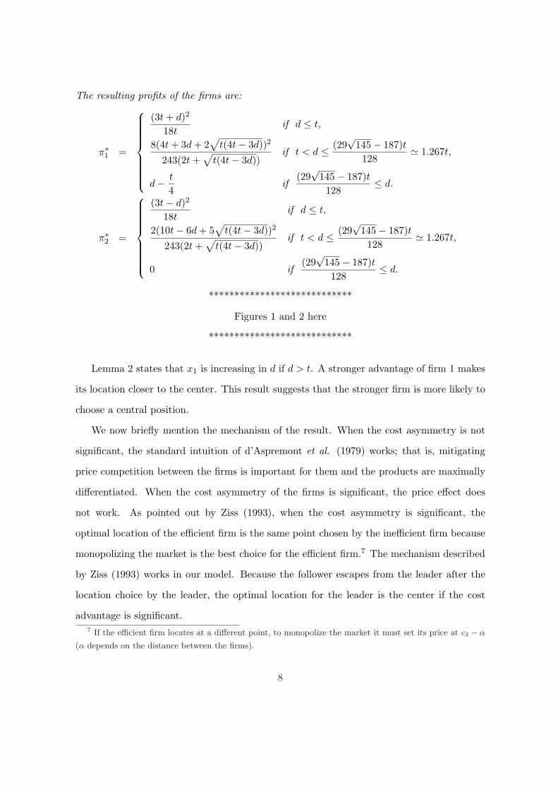
Lemma 2 states that x1 is increasing in d if d > t. A stronger advantage of firm 1 makes

its location closer to the center. This result suggests that the stronger firm is more likely to

choose a central position.

We now briefly mention the mechanism of the result. When the cost asymmetry is not

significant, the standard intuition of d’Aspremont et al. (1979) works; that is, mitigating

price competition between the firms is important for them and the products are maximally

differentiated. When the cost asymmetry of the firms is significant, the price effect does

not work. As pointed out by Ziss (1993), when the cost asymmetry is significant, the

optimal location of the efficient firm is the same point chosen by the inefficient firm because

monopolizing the market is the best choice for the efficient firm.7 The mechanism described

by Ziss (1993) works in our model. Because the follower escapes from the leader after the

location choice by the leader, the optimal location for the leader is the center if the cost

advantage is significant.7 If the efficient firm locates at a different point, to monopolize the market it must set its price at c2 − α

(α depends on the distance between the firms).

8

3.2 Consumer surplus and social welfare

From (6), (7), and Lemmas 1 and 2, we have the equilibrium quantity supplied by firm 1

and the equilibrium prices of the firms as follows:

D∗1 =

3t + d

6tif d ≤ t,

2(4t−√

t(4t− 3d)9t

if t < d < (29√

145−187)t128 ,

1 if (29√

145−187)t128 ≤ d.

(9)

p∗1 =

3t + 3c + d

3if d ≤ t,

27c + 12d + 16t + 8√

t(4t− 3d)27

if t < d < (29√

145−187)t128 ,

4c + 4d− t

4if (29

√145−187)t128 ≤ d.

(10)

p∗2 =

3t + 3c + 2d

3if d ≤ t,

27c + 15d + 20t + 10√

t(4t− 3d)27

if t < d < (29√

145−187)t128 ,

c + d if (29√

145−187)t128 ≤ d.

(11)

****************************

Figure 3 here

****************************

Figure 3 indicates that the sum of the marginal costs (2c + d) is not always correlated

with the equilibrium prices. This property is different from the standard Cournot model

(Salant and Shaffer (1999)).

9

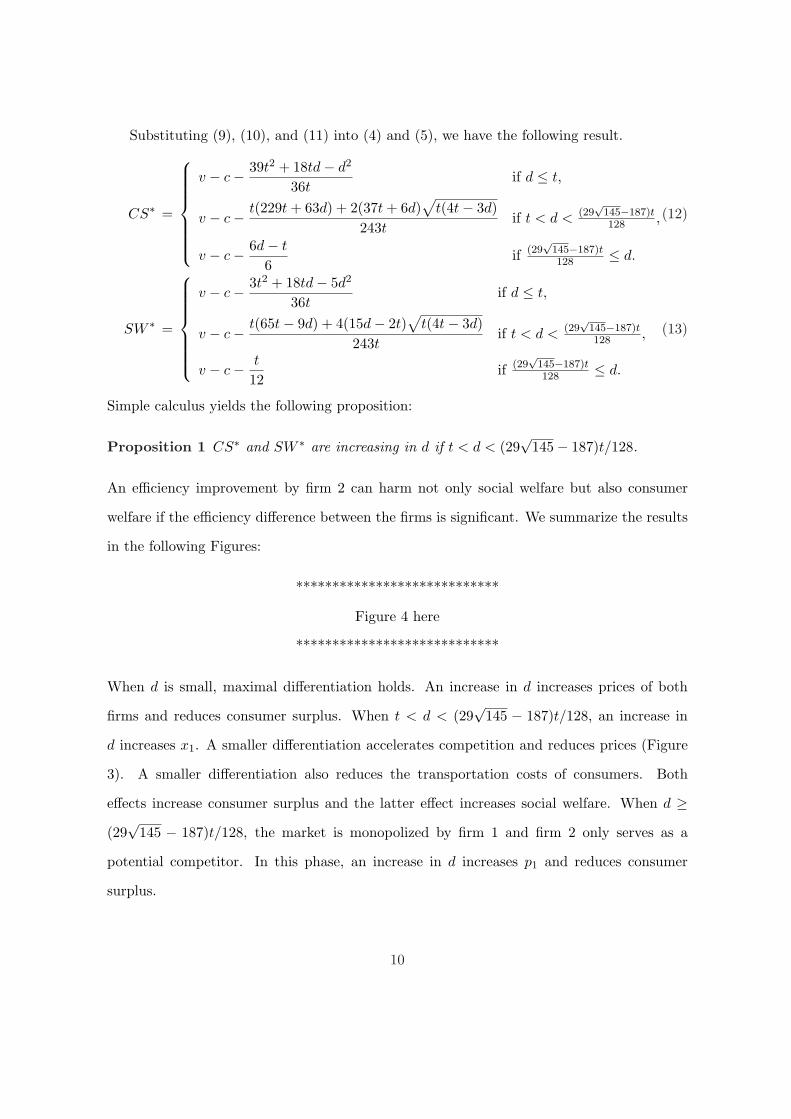
Substituting (9), (10), and (11) into (4) and (5), we have the following result.

CS∗ =

v − c− 39t2 + 18td− d2

36tif d ≤ t,

v − c− t(229t + 63d) + 2(37t + 6d)√

t(4t− 3d)243t

if t < d < (29√

145−187)t128 ,

v − c− 6d− t

6if (29

√145−187)t128 ≤ d.

(12)

SW ∗ =

v − c− 3t2 + 18td− 5d2

36tif d ≤ t,

v − c− t(65t− 9d) + 4(15d− 2t)√

t(4t− 3d)243t

if t < d < (29√

145−187)t128 ,

v − c− t

12if (29

√145−187)t128 ≤ d.

(13)

Simple calculus yields the following proposition:

Proposition 1 CS∗ and SW ∗ are increasing in d if t < d < (29√

145− 187)t/128.

An efficiency improvement by firm 2 can harm not only social welfare but also consumer

welfare if the efficiency difference between the firms is significant. We summarize the results

in the following Figures:

****************************

Figure 4 here

****************************

When d is small, maximal differentiation holds. An increase in d increases prices of both

firms and reduces consumer surplus. When t < d < (29√

145 − 187)t/128, an increase in

d increases x1. A smaller differentiation accelerates competition and reduces prices (Figure

3). A smaller differentiation also reduces the transportation costs of consumers. Both

effects increase consumer surplus and the latter effect increases social welfare. When d ≥(29√

145 − 187)t/128, the market is monopolized by firm 1 and firm 2 only serves as a

potential competitor. In this phase, an increase in d increases p1 and reduces consumer

surplus.

10

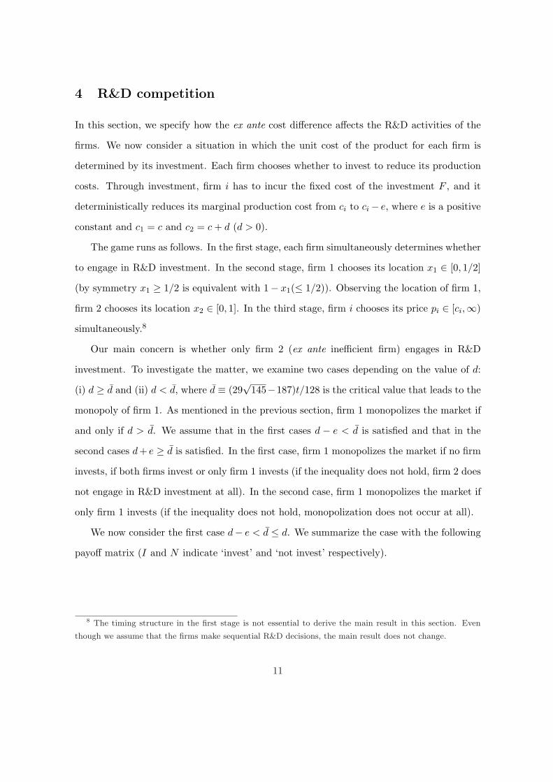
4 R&D competition

In this section, we specify how the ex ante cost difference affects the R&D activities of the

firms. We now consider a situation in which the unit cost of the product for each firm is

determined by its investment. Each firm chooses whether to invest to reduce its production

costs. Through investment, firm i has to incur the fixed cost of the investment F , and it

deterministically reduces its marginal production cost from ci to ci− e, where e is a positive

constant and c1 = c and c2 = c + d (d > 0).

The game runs as follows. In the first stage, each firm simultaneously determines whether

to engage in R&D investment. In the second stage, firm 1 chooses its location x1 ∈ [0, 1/2]

(by symmetry x1 ≥ 1/2 is equivalent with 1− x1(≤ 1/2)). Observing the location of firm 1,

firm 2 chooses its location x2 ∈ [0, 1]. In the third stage, firm i chooses its price pi ∈ [ci,∞)

simultaneously.8

Our main concern is whether only firm 2 (ex ante inefficient firm) engages in R&D

investment. To investigate the matter, we examine two cases depending on the value of d:

(i) d ≥ d̄ and (ii) d < d̄, where d̄ ≡ (29√

145−187)t/128 is the critical value that leads to the

monopoly of firm 1. As mentioned in the previous section, firm 1 monopolizes the market if

and only if d > d̄. We assume that in the first cases d − e < d̄ is satisfied and that in the

second cases d+ e ≥ d̄ is satisfied. In the first case, firm 1 monopolizes the market if no firm

invests, if both firms invest or only firm 1 invests (if the inequality does not hold, firm 2 does

not engage in R&D investment at all). In the second case, firm 1 monopolizes the market if

only firm 1 invests (if the inequality does not hold, monopolization does not occur at all).

We now consider the first case d− e < d̄ ≤ d. We summarize the case with the following

payoff matrix (I and N indicate ‘invest’ and ‘not invest’ respectively).

8 The timing structure in the first stage is not essential to derive the main result in this section. Even

though we assume that the firms make sequential R&D decisions, the main result does not change.

11

Firm 1 / Firm 2 I N

I −F 04d− t

4− F

4d + 4e− t

4− F

N πf2 (N, I)− F 0

πf1 (N, I)

4d− t

4

where

πf1 (N, I) ≡ 8(4t + 3(d− e) + 2

√t(4t− 3(d− e)))2

243(2t +√

t(4t− 3(d− e))),

πf2 (N, I) ≡ 2(10t− 6(d− e) + 5

√t(4t− 3(d− e)))2

243(2t +√

t(4t− 3(d− e))).

As mentioned earlier, our main concern in this section is whether (N, I) is the unique

equilibrium outcome. We now derive the condition that only (N, I) appears in equilibrium.

After some calculus, we have the following proposition:

Proposition 2 Suppose that d − e < d̄ ≤ d (the first case). Then (N, I) is the unique

equilibrium outcome if and only if e < F < πf2 (N, I).

If e ≥ πf2 (N, I), (N, I) never becomes the unique equilibrium outcome. Figure 5 describes

the regions where e < πf2 (N, I) is satisfied.

****************************

Figure 5 here

****************************

Proposition 2 states that the incentive of the minor firm for R&D investment can be

stronger than that of the major firm. We explain the intuition in the last paragraph of this

section.

We now consider the second case, d < d̄ ≤ d + e. We summarize the case with the

following payoff matrix (I and N indicate ‘invest’ and ‘not invest’ respectively).

12

Firm 1 / Firm 2 I N

I πs2(N,N)− F 0

πs1(N, N)− F

4(d + e)− t

4− F

N πs2(N, I)− F πs

2(N, N)πs

1(N, I) πs1(N, N)

where

πs1(N, N) ≡ 8(4t + 3d + 2

√t(4t− 3d))2

243(2t +√

t(4t− 3d)),

πs2(N, N) ≡ 2(10t− 6d + 5

√t(4t− 3d))2

243(2t +√

t(4t− 3d)),

πs1(N, I) ≡ 8(4t + 3(d− e) + 2

√t(4t− 3(d− e)))2

243(2t +√

t(4t− 3(d− e))),

πs2(N, I) ≡ 2(10t− 6(d− e) + 5

√t(4t− 3(d− e)))2

243(2t +√

t(4t− 3(d− e))).

After some calculus, we have the following proposition:

Proposition 3 Suppose that d < d̄ ≤ d + e (the second case). Then (N, I) is the unique

equilibrium outcome if and only if

πs1(N,N)− πs

1(N, I) < F < min{πs2(N, N), πs

2(N, I)− πs2(N, N)}. (14)

If πs1(N, N)− πs

1(N, I) ≥ min{πs2(N, N), πs

2(N, I)− πs2(N, N)}, there is no F satisfying (14).

Figure 6 indicates regions where πs1(N, N)−πs

1(N, I) < min{πs2(N,N), πs

2(N, I)−πs2(N,N)}

is satisfied. In regions (1), (2), and (3) in Figure 6, this inequality is satisfied.

****************************

Figure 6 here

****************************

As we stated in the previous section, when the cost difference d lies on (t, (29√

145 −187)t/128), a decrease in the marginal cost of firm 2 (resp. firm 1) is harmful (resp. bene-

ficial) for consumers and social welfare. Nevertheless, it is possible that firm 2 has stronger

incentives for cost-reducing R&D investment. A decrease in cost for firm 2 increases the

13

degree of product differentiation, resulting in an increase in the market share of firm 2 and

increases in the prices. Both effects enhance the profit of firm 2, thus, firm 2 has a strong

incentive for R&D investment for strategic purposes. In contrast, a decrease in the marginal

cost of firm 1 decreases the degree of product differentiation, resulting in an increase in the

market share of firm 1 but a decrease in prices. The former effect increases the profit of firm

1 and the latter decreases the profit of firm 1. Thus, firm 1 has a smaller strategic incentive

for R&D investment than firm 2.

On the other hand, there is an economy of scale in R&D. This is because the benefit of

cost reduction is proportional to its market share, whereas the investment cost F does not

depend on market share. For this economy of scale effect, firm 1 has a stronger incentive for

R&D. The strategic effect mentioned above can dominate this economy of scale effect. This

is why (N, I) can be the unique equilibrium. This result is also in sharp contrast with the

existing result presented in Lahiri and Ono (1999).9

Remark Because of mathematical complexity, we have investigated the R&D competition

with the specific form of investment technologies. To show the generality of our result, we

now present the marginal gains from a marginal cost reduction. The gains are derived by the

partial differentiations of πi (i = 1, 2) with respect to d. The absolute value of each firm’s

partial differentiation presents the significance of the marginal gain from its marginal cost

reduction given the cost difference between the firms, d. To derive the marginal gain, we use

πi (i = 1, 2) in Lemma 2. Simple calculus leads to the following (we ignore the discontinuities

9 The economy of scale effect is common in other R&D literature such as Lahiri and Ono (1999). Our

two strategic elements discussed in the text are quite different from those of existing works and yield our

contrasting result.

14

of the profit functions).

∣∣∣∣∂π∗1∂d

∣∣∣∣ =

3t + d

9tif d ≤ t,

4t(4(2t +√

t(4t− 3d))2 − 9d2)27

√t(4t− 3d)(2t +

√t(4t− 3d))2

if t < d ≤ d̄,

1 if d̄ ≤ d.

∣∣∣∣∂π∗2∂d

∣∣∣∣ =

3t− d

9tif d ≤ t,

t(6d− 5(2t +√

t(4t− 3d)))(6d− 7(2t +√

t(4t− 3d)))27

√t(4t− 3d)(2t +

√t(4t− 3d))2

if t < d ≤ d̄,

0 if d̄ ≤ d.

This is summarized in Figure 7 (note that, t is normalized to 1 without loss of generality).

****************************

Figure 7 here

****************************

We easily find that the marginal gain of firm 2 from the marginal cost reduction is larger

than that of firm 1 when t < d < d̄. As mentioned earlier, this property stems from the

relation between the cost difference and the degree of product differentiation.

5 Concluding remarks

In this paper, we use a location model and show that helping the minor firm reduces not only

social welfare but also consumer surplus. In their pioneering work, Lahiri and Ono (1988)

show that helping a minor firm can reduce welfare. However, in their models, a decrease

in costs for the inferior firm increases consumer surplus. Our result makes a sharp contrast

with theirs because we show that helping a minor firm can reduce consumer surplus.

We also discuss R&D incentives of firms. Lahiri and Ono (1999) and Kitahara and

Matsumura (2006) have already stated that the incentive for R&D of the superior firm

(inferior firm) is insufficient (excessive) from the viewpoint of social welfare. However, in

their model, the superior firm has a stronger incentive for R&D than the inferior firm. We

15

show that the incentive of the inferior firm for R&D can be larger than the superior firm

when a decrease in the inferior firm’s cost reduces both consumer surplus and total surplus.

This also makes a sharp contrast with the previous results mentioned above.

A cost difference between these firms can appear in various contexts. One important

example is international competition under import tariffs. Another example is in the context

of vertical foreclosure, where a vertically integrated firm faces a smaller input price than

the independent downstream firms. Applying our principle to these contexts remains an

interesting research agenda for future research.

16

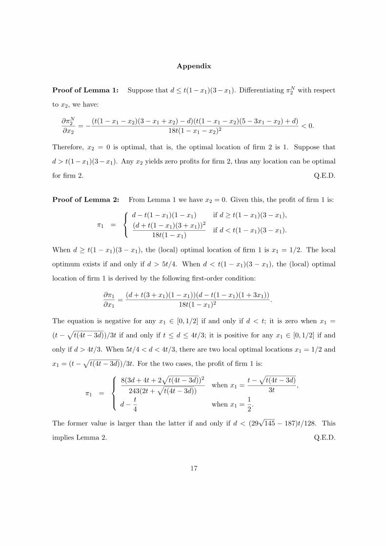
Appendix

Proof of Lemma 1: Suppose that d ≤ t(1−x1)(3−x1). Differentiating πN2 with respect

to x2, we have:

∂πN2

∂x2= −(t(1− x1 − x2)(3− x1 + x2)− d)(t(1− x1 − x2)(5− 3x1 − x2) + d)

18t(1− x1 − x2)2< 0.

Therefore, x2 = 0 is optimal, that is, the optimal location of firm 2 is 1. Suppose that

d > t(1−x1)(3−x1). Any x2 yields zero profits for firm 2, thus any location can be optimal

for firm 2. Q.E.D.

Proof of Lemma 2: From Lemma 1 we have x2 = 0. Given this, the profit of firm 1 is:

π1 =

d− t(1− x1)(1− x1) if d ≥ t(1− x1)(3− x1),(d + t(1− x1)(3 + x1))2

18t(1− x1)if d < t(1− x1)(3− x1).

When d ≥ t(1 − x1)(3 − x1), the (local) optimal location of firm 1 is x1 = 1/2. The local

optimum exists if and only if d > 5t/4. When d < t(1 − x1)(3 − x1), the (local) optimal

location of firm 1 is derived by the following first-order condition:

∂π1

∂x1=

(d + t(3 + x1)(1− x1))(d− t(1− x1)(1 + 3x1))18t(1− x1)2

.

The equation is negative for any x1 ∈ [0, 1/2] if and only if d < t; it is zero when x1 =

(t −√

t(4t− 3d))/3t if and only if t ≤ d ≤ 4t/3; it is positive for any x1 ∈ [0, 1/2] if and

only if d > 4t/3. When 5t/4 < d < 4t/3, there are two local optimal locations x1 = 1/2 and

x1 = (t−√

t(4t− 3d))/3t. For the two cases, the profit of firm 1 is:

π1 =

8(3d + 4t + 2√

t(4t− 3d))2

243(2t +√

t(4t− 3d))when x1 =

t−√

t(4t− 3d)3t

,

d− t

4when x1 =

12.

The former value is larger than the latter if and only if d < (29√

145 − 187)t/128. This

implies Lemma 2. Q.E.D.

17

0.2 0.4 0.6 0.8 1 1.2 1.4d�t

0.1

0.2

0.3

0.4

0.5

x1

Figure 1: The optimal location of firm 1

Horizontal: d/t, Vertical: x1

18

0.2 0.4 0.6 0.8 1 1.2 1.4d�t

0.2

0.4

0.6

0.8

1

1.2

Πi

Π1

Π2

Figure 2: The profits of the firms

Horizontal: d/t, Vertical: πi (i = 1, 2)

19

0.2 0.4 0.6 0.8 1 1.2d�t

1.1

1.2

1.3

1.4

1.5

1.6

p1-c

0.2 0.4 0.6 0.8 1 1.2d�t

1.1

1.2

1.3

1.4

1.5

1.6

p2-c

The price of firm 1 The price of firm 2

Figure 3: The equilibrium Prices

Horizontal: d/t, Vertical: p∗i − c

20

0.2 0.4 0.6 0.8 1 1.2d�t

-1.4

-1.3

-1.2

-1.1

CS-Hv-cL

0.2 0.4 0.6 0.8 1 1.2d�t

-0.45

-0.35

-0.3

-0.25

-0.2

-0.15

-0.1

SW-Hv-cL

Consumer surplus Social welfare

Figure 4: Consumer surplus and social welfare

Horizontal: d/t, Vertical: CS∗ − (v − c) and SW ∗ − (v − c)

21

1.28 1.32 1.34 1.36 1.38 1.4 1.42d

0.025

0.05

0.075

0.1

0.125

0.15

e

d-e > d�

Πf2HN,IL>e

Πf2HN,IL<e

1.28 1.32 1.34 1.36 1.38 1.4 1.42d

0.025

0.05

0.075

0.1

0.125

0.15

e

Figure 5: Parameter range within which πf2 (N, I) > e holds.

22

1.1251.151.175 1.2 1.2251.25d

0.05

0.1

0.15

0.2

0.25

e

d-e<1

d+e<d�

H1L

H2L

H3L

H4L

1.1251.151.175 1.2 1.2251.25d

0.05

0.1

0.15

0.2

0.25

e

Figure 6: Parameter range within which Proposition 3 holds.

Note:(1) and (2) πs

1(N, N)− πs1(N, I) < πs

2(N, I)− πs2(N, N) < πs

2(N, N),(3) πs

1(N, N)− πs1(N, I) < πs

2(N, N) < πs2(N, I)− πs

2(N, N),(4) πs

2(N, N) < πs1(N,N)− πs

1(N, I) < πs2(N, I)− πs

2(N, N).

23

0.2 0.4 0.6 0.8 1 1.2d

0.1

0.2

0.3

0.4

0.5

0.6

ȶΠi�¶dÈ

¶Π2�¶d

¶Π1�¶d

Figure 7: The marginal gain from a marginal cost reduction

Horizontal: d, Vertical: |∂πi/∂d| (i = 1, 2).

24

References

Arrow, K. J. (1962). Economic welfare and the allocation of resources for invention. In:Nelson, R.R. (ed.), The Rate and Direction of Inventive Activity: Economic and SocialFactors, Princeton University Press, Princeton, 609–625.

Cohen, W. M. and Klepper, S. (1996). ‘A reprise of size and R&D’, Economic Journal, vol.106(437), pp. 925–51.

d’Aspremont, C., Gabszewicz, J.-J. and Thisse, J.-F. (1979). ‘On Hotelling’s stability incompetition’, Econometrica vol. 47(5), pp. 1145–50.

Hotelling, H. (1929). ‘Stability in competition’, Economic Journal, vol. 39, pp. 41–57.

Kitahara, M. and Matsumura, T. (2006). ‘Realized cost based subsidies for strategic R&Dinvestments with ex ante and ex post asymmetries’, Japanese Economic Review, vol.57(3), pp. 438–48.

Kitano, T. (2008). ‘Measuring the effects of tariff-jumping FDI on domestic and foreignfirms profits: a case of U.S. motorcycle industry, 1983-1987’, mimeo.

Lahiri, S. and Ono, Y. (1988). ‘Helping minor firms reduces welfare’, Economic Journal,vol. 98(393), pp. 1199–202.

Lahiri, S. and Ono, Y. (1997). ‘Asymmetric oligopoly, international trade, and welfare: asynthesis’, Journal of Economics, vol. 65(3), pp. 291–310.

Lahiri, S. and Ono, Y. (1998). ‘Foreign direct investment, local content requirement, andprofit taxation’, Economic Journal, vol. 108(447), pp. 444–57.

Lahiri, S. and Ono, Y. (1999). ‘R&D subsidies under asymmetric duopoly: a note’, JapaneseEconomic Review, vol. 50(1), pp. 104–11.

Liang, W. J. and Mai, C.-C. (2006). ‘Validity of the principle of minimum differentiationunder vertical subcontracting’, Regional Science and Urban Economics vol. 36(3), pp.373–84.

Matsumura, T. and Matsushima, N. (2009). ‘Cost differentials and mixed strategy equilibriain a Hotelling model’, Annals of Regional Science, vol. 43(1), pp. 215–34.

Meza, S. and Tombak, M. (forthcoming). ‘Endogenous location leadership’, InternationalJournal of Industrial Organization. http://dx.doi.org/10.1016/j.ijindorg.2009.03.001

Reid, P. C. (1991). Well Made in America: Lessons from Harley-Davidson on Being theBest. McGraw-Hill.

25

Rogers, M. (2004). ‘Networks, firm size and innovation’, Small Business Economics, vol.22(2), pp. 141–53.

Salant, S.W. and Shaffer, G. (1999). ‘Unequal treatment of identical agents in Cournotequilibrium’, American Economic Review, vol. 89(3), pp. 585–604.

Thomadsen, R. (2007). ‘Product positioning and competition: the role of location in thefast food industry’, Marketing Science, vol. 26, pp. 792–804.

Tirole, J. (1988). The Theory of Industrial Organization, MIT Press, Cambridge, MA.

Tyagi, R. (2000). ‘Sequential product positioning under differential costs’, ManagementScience, vol. 46, pp. 928–40.

Vickrey, W. S. (1964). Microstatics, Harcourt, Brace and World, New York.

Wang, X. H. and Zhao, J. (2007). ‘Welfare reductions from small cost reductions in differ-entiated oligopoly’, International Journal of Industrial Organization, vol. 25(1), pp.173–85.

Zhao, J. (2001). ‘A Characterization for the negative welfare effects of cost reduction inCournot oligopoly’, International Journal of Industrial Organization, vol. 19(3–4), pp.455–69.

Ziss, S. (1993). ‘Entry deterrence, cost advantage and horizontal product differentiation’,Regional Science and Urban Economics, vol. 23(4), pp. 523–43.

26