A six-lecture course - University of Cambridge · Floating Point Computation (slides 1–123) A...
123
UNIVERSITY OF CAMBRIDGE Floating Point Computation (slides 1–123) A six-lecture course D J Greaves (thanks to Alan Mycroft) Computer Laboratory, University of Cambridge http://www.cl.cam.ac.uk/teaching/current/FPComp Lent 2010–11 Floating Point Computation 1 Lent 2010–11
Transcript of A six-lecture course - University of Cambridge · Floating Point Computation (slides 1–123) A...
UNIVERSITY OF
CAMBRIDGE
Floating Point Computation(slides 1–123)
A six-lecture course
D J Greaves (thanks to Alan Mycroft)
Computer Laboratory, University of Cambridge
http://www.cl.cam.ac.uk/teaching/current/FPComp
Lent 2010–11
Floating Point Computation 1 Lent 2010–11
UNIVERSITY OF
CAMBRIDGE
A Few Cautionary Tales
The main enemy of this course is the simple phrase
“the computer calculated it, so it must be right”.
We’re happy to be wary for integer programs, e.g. having unit tests to
check that
sorting [5,1,3,2] gives [1,2,3,5],
but then we suspend our belief for programs producing real-number
values, especially if they implement a “mathematical formula”.
Floating Point Computation 2 Lent 2010–11
UNIVERSITY OF
CAMBRIDGE
Global Warming
Apocryphal story – Dr X has just produced a new climate modelling
program.
Interviewer: what does it predict?
Dr X: Oh, the expected 2–4◦C rise in average temperatures by 2100.
Interviewer: is your figure robust?
. . .
Floating Point Computation 3 Lent 2010–11

UNIVERSITY OF
CAMBRIDGE
Global Warming (2)
Apocryphal story – Dr X has just produced a new climate modelling
program.
Interviewer: what does it predict?
Dr X: Oh, the expected 2–4◦C rise in average temperatures by 2100.
Interviewer: is your figure robust?
Dr X: Oh yes, indeed it gives results in the same range even if the input
data is randomly permuted . . .
We laugh, but let’s learn from this.
Floating Point Computation 4 Lent 2010–11
UNIVERSITY OF
CAMBRIDGE
Global Warming (3)
What could cause this sort or error?
• the wrong mathematical model of reality (most subject areas lack
models as precise and well-understood as Newtonian gravity)
• a parameterised model with parameters chosen to fit expected
results (‘over-fitting’)
• the model being very sensitive to input or parameter values
• the discretisation of the continuous model for computation
• the build-up or propagation of inaccuracies caused by the finite
precision of floating-point numbers
• plain old programming errors
We’ll only look at the last four, but don’t forget the first two.
Floating Point Computation 5 Lent 2010–11

UNIVERSITY OF
CAMBRIDGE
Real world examples
Find Kees Vuik’s web page “Computer Arithmetic Tragedies” for these
and more:
• Patriot missile interceptor fails to intercept due to 0.1 second being
the ‘recurring decimal’ 0.00 1100 1100 . . .2 in binary (1991)
• Ariane 5 $500M firework display caused by overflow in converting
64-bit floating-point number to 16-bit integer (1996)
• The Sleipner A offshore oil platform sank . . . post-accident
investigation traced the error to inaccurate finite element
approximation of the linear elastic model of the tricell (using the
popular finite element program NASTRAN). The shear stresses were
underestimated by 47% . . .
Learn from the mistakes of the past . . .
Floating Point Computation 6 Lent 2010–11

UNIVERSITY OF
CAMBRIDGE
Overall motto: threat minimisation
• Algorithms involving floating point (float and double in Java and
C, [misleadingly named] real in ML and Fortran) pose a significant
threat to the programmer or user.
• Learn to distrust your own naıve coding of such algorithms, and,
even more so, get to distrust others’.
• Start to think of ways of sanity checking (by human or machine)
any floating point value arising from a computation, library or
package—unless its documentation suggests an attention to detail
at least that discussed here (and even then treat with suspicion).
• Just because the “computer produces a numerical answer” doesn’t
mean this has any relationship to the ‘correct’ answer.
Here be dragons!
Floating Point Computation 7 Lent 2010–11
UNIVERSITY OF
CAMBRIDGE
What’s this course about?
• How computers represent and calculate with ‘real number’ values.
• What problems occur due to the values only being finite (both range
and precision).
• How these problems add up until you get silly answers.
• How you can stop your programs and yourself from looking silly
(and some ideas on how to determine whether existing programs
have been silly).
• Chaos and ill-conditionedness.
• Knowing when to call in an expert—remember there is 50+ years of
knowledge on this and you only get 6 lectures from me.
Floating Point Computation 8 Lent 2010–11

UNIVERSITY OF
CAMBRIDGE
Part 1
Introduction/reminding you what you
already know
Floating Point Computation 9 Lent 2010–11
UNIVERSITY OF
CAMBRIDGE
Reprise: signed and unsigned integers
An 8-bit value such as 10001011 can naturally be interpreted as either
an signed number (27 + 23 + 21 + 20 = 139) or as a signed number
(−27 + 23 + 21 + 20 = −117).
This places the decimal (binary!?!) point at the right-hand end. It could
also be interpreted as a fixed-point number by imagining a decimal point
elsewhere (e.g. in the middle to get) 1000.1011; this would have value
23 + 2−1 + 2−3 + 2−4 = 8 1116 = 8.6875.
(The above is an unsigned fixed-point value for illustration, normally we
use signed fixed-point values.)
Floating Point Computation 10 Lent 2010–11
UNIVERSITY OF
CAMBRIDGE
Fixed point values and saturating arithmetic
Fixed-point values are often useful (e.g. in low-power/embedded devices)
but they are prone to overflow. E.g. 2*10001011 = 00010110 so
2*8.6875 = 1.375!! One alternative is to make operations saturating so
that 2*10001011 = 11111111 which can be useful (e.g. in audio). Note
1111.11112 = 15.937510.
An alternative way to avoid this sort of overflow is to allow the decimal
point to be determined at run-time (by another part of the value)
“floating point” instead of being fixed (independent of the value as
above) “fixed point” – the subject of this course.
Floating Point Computation 11 Lent 2010–11
UNIVERSITY OF
CAMBRIDGE
Back to school
Scientific notation (from Wikipedia, the free encyclopedia)
In scientific notation, numbers are written using powers of ten in the
form a × 10b where b is an integer exponent and the coefficient a is any
real number, called the significand or mantissa.
In normalised form, a is chosen such that 1 ≤ a < 10. It is implicitly
assumed that scientific notation should always be normalised except
during calculations or when an unnormalised form is desired.
What Wikipedia should say: zero is problematic—its exponent doesn’t
matter and it can’t be put in normalised form.
Floating Point Computation 12 Lent 2010–11
UNIVERSITY OF
CAMBRIDGE
Back to school (2)
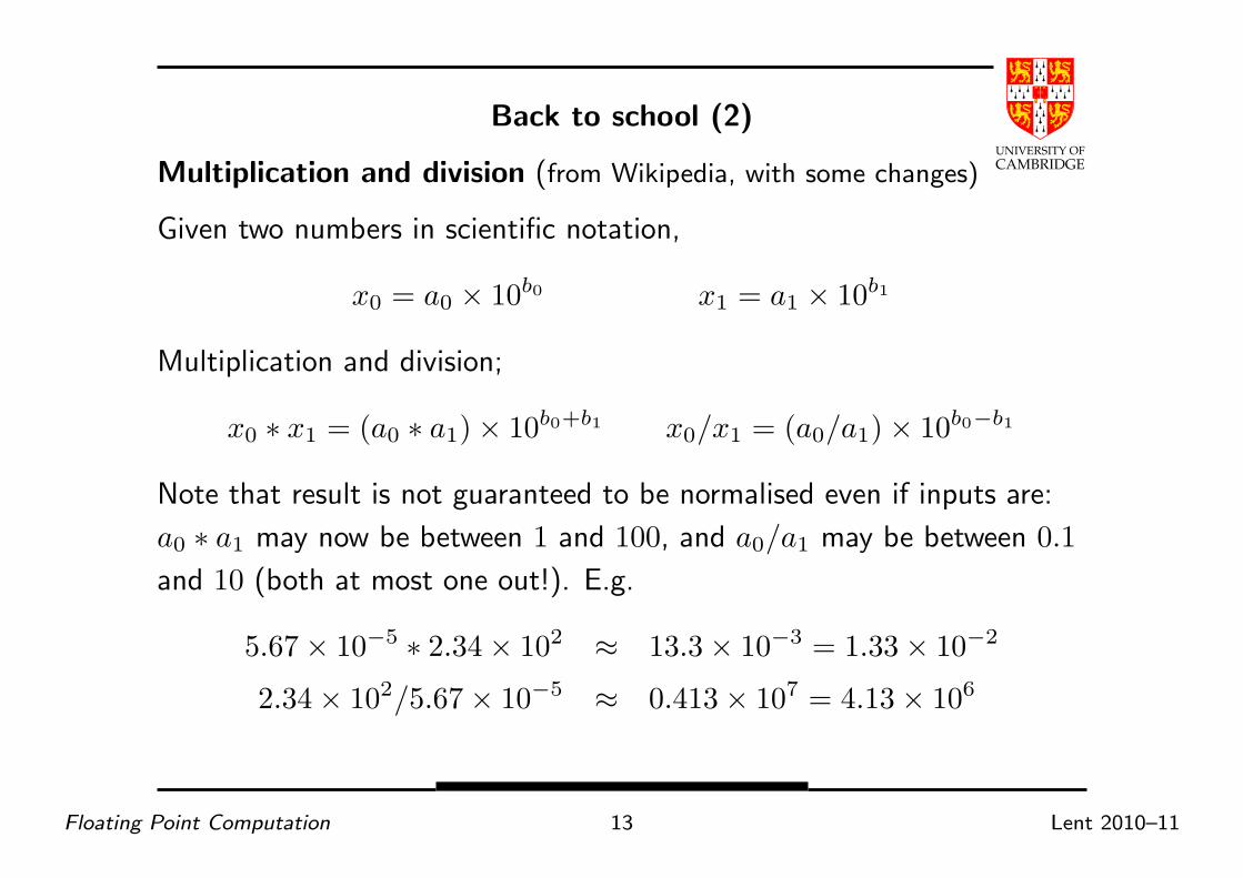
Multiplication and division (from Wikipedia, with some changes)
Given two numbers in scientific notation,
x0 = a0 × 10b0 x1 = a1 × 10b1
Multiplication and division;
x0 ∗ x1 = (a0 ∗ a1) × 10b0+b1 x0/x1 = (a0/a1) × 10b0−b1
Note that result is not guaranteed to be normalised even if inputs are:
a0 ∗ a1 may now be between 1 and 100, and a0/a1 may be between 0.1
and 10 (both at most one out!). E.g.
5.67 × 10−5 ∗ 2.34 × 102 ≈ 13.3 × 10−3 = 1.33 × 10⁻²
2.34 × 10²/5.67 × 10−5 ≈ 0.413 × 107 = 4.13 × 10⁶
Floating Point Computation 13 Lent 2010–11

UNIVERSITY OF
CAMBRIDGE
Back to school (3)
Addition and subtraction require the numbers to be represented using
the same exponent, normally the bigger of b0 and b1.
W.l.o.g. b0 > b1, so write x1 = (a1 ∗ 10b1−b0) × 10b0 (a shift!) and
add/subtract the mantissas.
x0 ± x1 = (a0 ± (a1 ∗ 10b1−b0)) × 10b0
E.g.
2.34× 10⁻⁵ + 5.67× 10−6 = 2.34× 10⁻⁵ + 0.567× 10⁻⁵ ≈ 2.91× 10⁻⁵
A cancellation problem we will see more of:
2.34 × 10⁻⁵ − 2.33 × 10−5 = 0.01 × 10−5 = 1.00 × 10⁻⁷
When numbers reinforce (e.g. add with same-sign inputs) new mantissa
is in range [1, 20), when they cancel it is in range [0..10). After
cancellation we may require several shifts to normalise.
Floating Point Computation 14 Lent 2010–11
UNIVERSITY OF
CAMBRIDGE
Significant figures can mislead
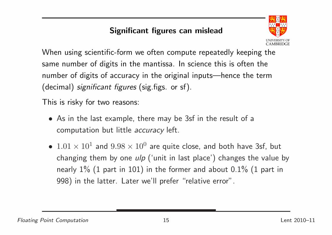
When using scientific-form we often compute repeatedly keeping the
same number of digits in the mantissa. In science this is often the
number of digits of accuracy in the original inputs—hence the term
(decimal) significant figures (sig.figs. or sf).
This is risky for two reasons:
• As in the last example, there may be 3sf in the result of a
computation but little accuracy left.
• 1.01 × 101 and 9.98 × 100 are quite close, and both have 3sf, but
changing them by one ulp (‘unit in last place’) changes the value by
nearly 1% (1 part in 101) in the former and about 0.1% (1 part in
998) in the latter. Later we’ll prefer “relative error”.
Floating Point Computation 15 Lent 2010–11
UNIVERSITY OF
CAMBRIDGE
Significant figures can mislead (2)
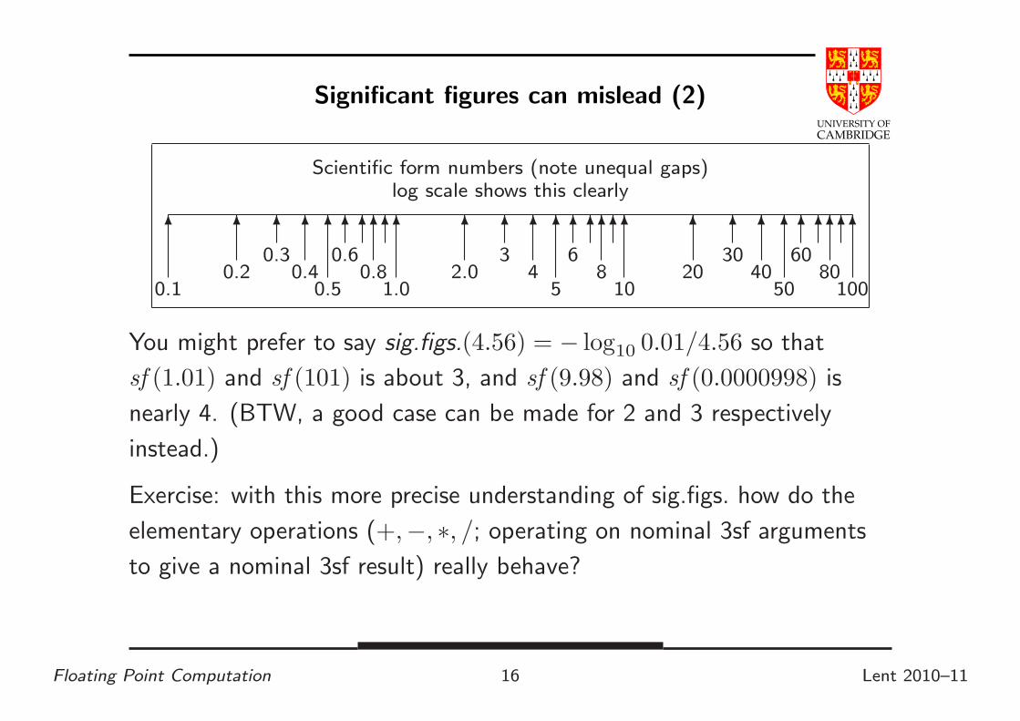
Scientific form numbers (note unequal gaps)log scale shows this clearly
6
0.1
6
0.2
60.3
6
0.4
6
0.5
60.6
66
0.8
66
1.0
6
2.0
63
6
4
6
5
66
66
8
66
10
6
20
630
6
40
6
50
660
66
80
66
100
You might prefer to say sig.figs.(4.56) = − log10 0.01/4.56 so that
sf (1.01) and sf (101) is about 3, and sf (9.98) and sf (0.0000998) is
nearly 4. (BTW, a good case can be made for 2 and 3 respectively
instead.)
Exercise: with this more precise understanding of sig.figs. how do the
elementary operations (+,−, ∗, /; operating on nominal 3sf arguments
to give a nominal 3sf result) really behave?
Floating Point Computation 16 Lent 2010–11
UNIVERSITY OF
CAMBRIDGE
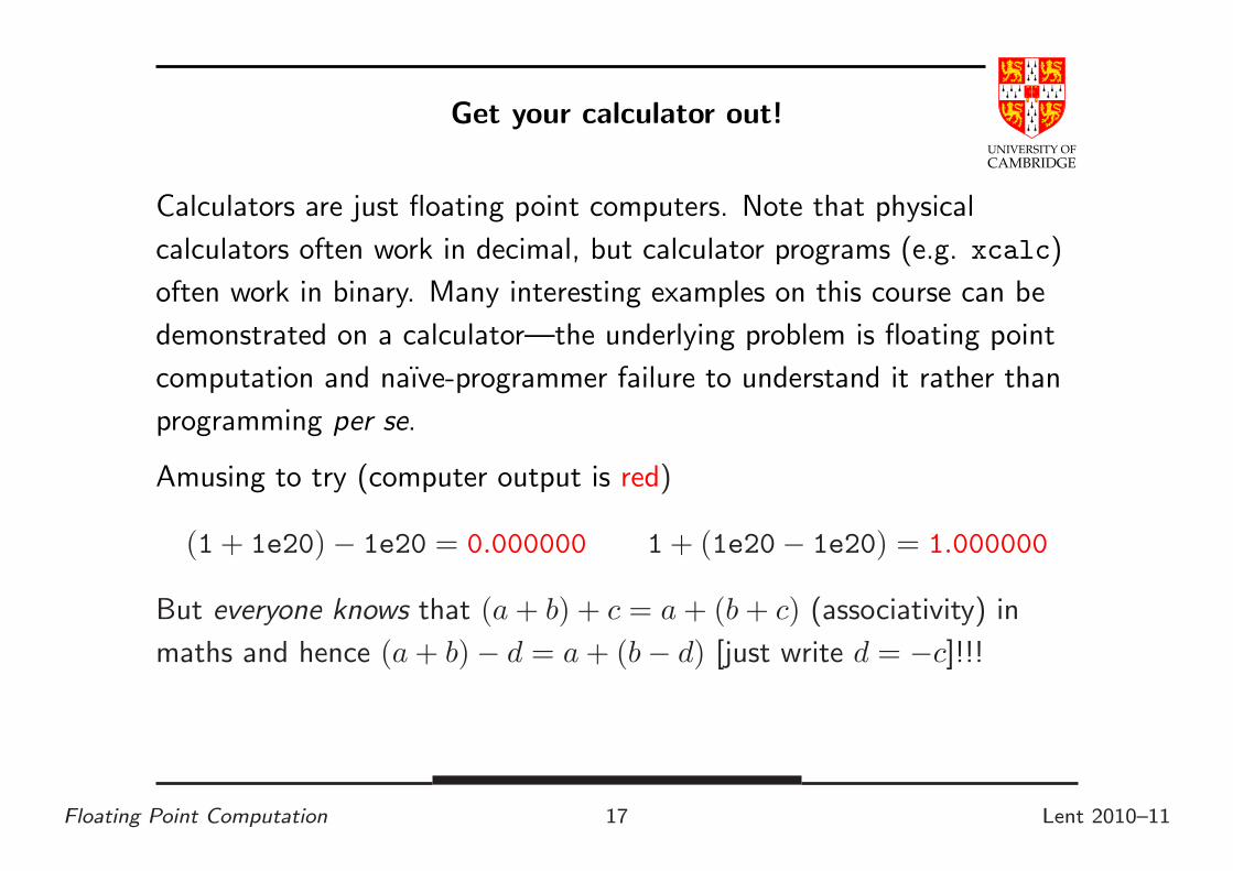
Get your calculator out!
Calculators are just floating point computers. Note that physical
calculators often work in decimal, but calculator programs (e.g. xcalc)
often work in binary. Many interesting examples on this course can be
demonstrated on a calculator—the underlying problem is floating point
computation and naıve-programmer failure to understand it rather than
programming per se.
Amusing to try (computer output is red)
(1 + 1e20) − 1e20 = 0.000000 1 + (1e20− 1e20) = 1.000000
But everyone knows that (a + b) + c = a + (b + c) (associativity) in
maths and hence (a + b) − d = a + (b − d) [just write d = −c]!!!
Floating Point Computation 17 Lent 2010–11
UNIVERSITY OF
CAMBRIDGE
Get your calculator out (2)
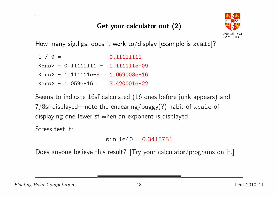
How many sig.figs. does it work to/display [example is xcalc]?
1 / 9 = 0.11111111
<ans> - 0.11111111 = 1.111111e-09
<ans> - 1.111111e-9 = 1.059003e-16
<ans> - 1.059e-16 = 3.420001e-22
Seems to indicate 16sf calculated (16 ones before junk appears) and
7/8sf displayed—note the endearing/buggy(?) habit of xcalc of
displaying one fewer sf when an exponent is displayed.
Stress test it:
sin 1e40 = 0.3415751
Does anyone believe this result? [Try your calculator/programs on it.]
Floating Point Computation 18 Lent 2010–11
UNIVERSITY OF
CAMBRIDGE
Computer Representation
A computer representation must be finite. If we allocate a fixed size of
storage for each then we need to
• fix a size of mantissa (sig.figs.)
• fix a size for exponent (exponent range)
We also need to agree what the number means, e.g. agreeing the base
used by the exponent.
Why “floating point”? Because the exponent logically determines where
the decimal point is placed within (or even outside) the mantissa. This
originates as an opposite of “fixed point” where a 32-bit integer might
be treated as having a decimal point between (say) bits 15 and 16.
Floating point can simple be thought of simply as (a subset of all
possible) values in scientific notation held in a computer.
Floating Point Computation 19 Lent 2010–11
UNIVERSITY OF
CAMBRIDGE
Computer Representation (2)
Nomenclature. Given a number represented as βe × d0.d1 · · · dp−1 we
call β the base (or radix) and p the precision.
Note that (β = 2, p = 24) may be less accurate than (β = 10, p = 10).
Now let’s turn to binary representations (β = 2, as used on most modern
machines, will solely be considered in this course, but note the IBM/360
series of mainframes used β = 16 which gave some entertaining but
obsolete problems).
Floating Point Computation 20 Lent 2010–11

UNIVERSITY OF
CAMBRIDGE
Decimal or Binary?
Most computer arithmetic is in binary, as values are represented as 0’s
and 1’s. However, floating point values, even though they are
represented as bits, can use β = 2 or β = 10.
Most computer programs use the former. However, to some extent it is
non-intuitive for humans, especially for fractional numbers (e.g. that
0.110 is recurring when expressed in binary).
Most calculators work in decimal β = 10 to make life more intuitive, but
various software calculators work in binary (see xcalc above).
Microsoft Excel is a particular issue. It tries hard to give the illusion of
having floating point with 15 decimal digits, but internally it uses 64-bit
floating point. This gives rise to a fair bit of criticism and various users
with jam on their faces.
Floating Point Computation 21 Lent 2010–11

UNIVERSITY OF
CAMBRIDGE
Part 2
Floating point representation
Floating Point Computation 22 Lent 2010–11
UNIVERSITY OF
CAMBRIDGE
Standards
In the past every manufacturer produced their own floating point
hardware and floating point programs gave different answers. IEEE
standardisation fixed this.
There are two different IEEE standards for floating-point computation.
IEEE 754 is a binary standard that requires β = 2, p = 24 (number of
mantissa bits) for single precision and p = 53 for double precision. It
also specifies the precise layout of bits in a single and double precision.
[Edited quote from Goldberg.]
It has just (2008) been revised to include additional (longer) binary
floating point formats and also decimal floating formats.
IEEE 854 is more general and allows binary and decimal representation
without fixing the bit-level format.
Floating Point Computation 23 Lent 2010–11
UNIVERSITY OF
CAMBRIDGE
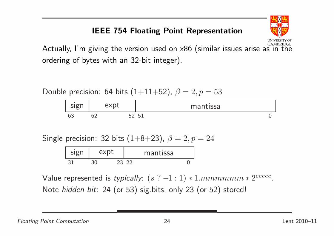
IEEE 754 Floating Point Representation
Actually, I’m giving the version used on x86 (similar issues arise as in the
ordering of bytes with an 32-bit integer).
Single precision: 32 bits (1+8+23), β = 2, p = 24
sign31
expt30 23
mantissa22 0
Double precision: 64 bits (1+11+52), β = 2, p = 53
sign63
expt62 52
mantissa51 0
Value represented is typically: (s ? −1 : 1) ∗ 1.mmmmmm ∗ 2eeeee.
Note hidden bit: 24 (or 53) sig.bits, only 23 (or 52) stored!
Floating Point Computation 24 Lent 2010–11
UNIVERSITY OF
CAMBRIDGE
Hidden bit and exponent representation
Advantage of base-2 (β = 2) exponent representation: all normalised
numbers start with a ’1’, so no need to store it. (Just like base 10, there
normalised numbers start 1..9, in base 2 they start 1..1.)
Floating Point Computation 25 Lent 2010–11
UNIVERSITY OF
CAMBRIDGE
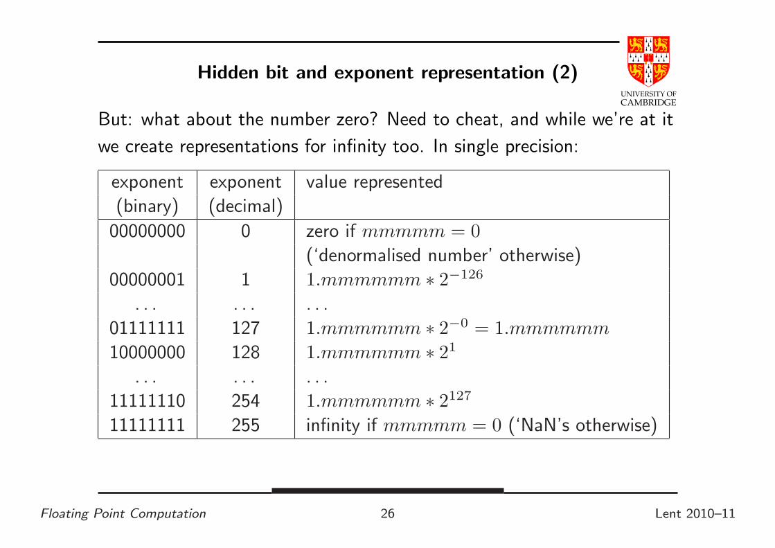
Hidden bit and exponent representation (2)
But: what about the number zero? Need to cheat, and while we’re at it
we create representations for infinity too. In single precision:
exponent exponent value represented
(binary) (decimal)
00000000 0 zero if mmmmm = 0
(‘denormalised number’ otherwise)
00000001 1 1.mmmmmm ∗ 2−126
. . . . . . . . .
01111111 127 1.mmmmmm ∗ 2−0 = 1.mmmmmm
10000000 128 1.mmmmmm ∗ 21
. . . . . . . . .
11111110 254 1.mmmmmm ∗ 2127
11111111 255 infinity if mmmmm = 0 (‘NaN’s otherwise)
Floating Point Computation 26 Lent 2010–11
UNIVERSITY OF
CAMBRIDGE
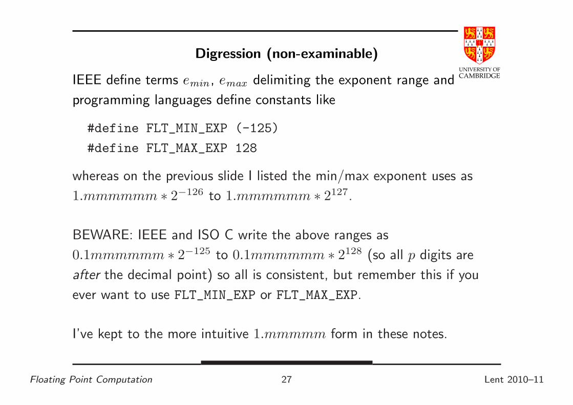
Digression (non-examinable)
IEEE define terms emin , emax delimiting the exponent range and
programming languages define constants like
#define FLT_MIN_EXP (-125)
#define FLT_MAX_EXP 128
whereas on the previous slide I listed the min/max exponent uses as
1.mmmmmm ∗ 2−126 to 1.mmmmmm ∗ 2127.
BEWARE: IEEE and ISO C write the above ranges as
0.1mmmmmm ∗ 2−125 to 0.1mmmmmm ∗ 2128 (so all p digits are
after the decimal point) so all is consistent, but remember this if you
ever want to use FLT_MIN_EXP or FLT_MAX_EXP.
I’ve kept to the more intuitive 1.mmmmm form in these notes.
Floating Point Computation 27 Lent 2010–11

UNIVERSITY OF
CAMBRIDGE
Hidden bit and exponent representation (3)
Double precision is similar, except that the 11-bit exponent field now
gives non-zero/non-infinity exponents ranging from 000 0000 0001
representing 2−1022 via 011 1111 1111 representing 20 to 111 1111 1110
representing 21023.
This representation is called “excess-127” (single) or “excess-1023”
(double precision).
Why use it?
Because it means that (for positive numbers, and ignoring NaNs)
floating point comparison is the same as integer comparison.
Why 127 not 128? The committee decided it gave a more symmetric
number range (see next slide).
Floating Point Computation 28 Lent 2010–11

UNIVERSITY OF
CAMBRIDGE
Solved exercises
What’s the smallest and biggest normalised numbers in single precision
IEEE floating point?
Biggest: exponent field is 0..255, with 254 representing 2127. The
biggest mantissa is 1.111...111 (24 bits in total, including the implicit
leading zero) so 1.111...111× 2127. Hence almost 2128 which is 28 ∗ 2120
or 256 ∗ 102412, i.e. around 3 ∗ 1038.
FLT_MAX from <float.h> gives 3.40282347e+38f.
Smallest? That’s easy: −3.40282347e+38! OK, I meant smallest
positive. I get 1.000...000 × 2−126 which is by similar reasoning around
16 × 2−130 or 1.6 × 10−38.
FLT_MIN from <float.h> gives 1.17549435e-38f.
Floating Point Computation 29 Lent 2010–11
UNIVERSITY OF
CAMBRIDGE
Solved exercises (2)
‘denormalised numbers’ can range down to 2−150 ≈ 1.401298e-45, but
there is little accuracy at this level.
And the precision of single precision? 223 is about 107, so in principle
7sf. (But remember this is for representing a single number, operations
will rapidly chew away at this.)
And double precision? DBL MAX 1.79769313486231571e+308 and
DBL MIN 2.22507385850720138e-308 with around 16sf.
How many single precision floating point numbers are there?
Answer: 2 signs * 254 exponents * 223 mantissas for normalised
numbers plus 2 zeros plus 2 infinities (plus NaNs and denorms not
covered in this course).
Floating Point Computation 30 Lent 2010–11
UNIVERSITY OF
CAMBRIDGE
Solved exercises (3)
Which values are representable exactly as normalised single precision
floating point numbers?
Legal Answer: ± ((223 + i)/223) × 2j where 0 ≤ i < 223 and
−126 ≤ j ≤ 127 (because of hidden bit)
More Useful Answer: ± i × 2j where 0 ≤ i < 224 and
−126 − 23 ≤ j ≤ 127 − 23
(but legally only right for j < −126 if we also include denormalised
numbers):
Compare: what values are exactly representable in normalised 3sf
decimal? Answer: i × 10j where 100 ≤ i ≤ 999.
Floating Point Computation 31 Lent 2010–11
UNIVERSITY OF
CAMBRIDGE
Solved exercises (4)
So you mean 0.1 is not exactly representable? Its nearest single precision
IEEE number is the recurring ‘decimal’ 0x3dcccccd (note round to
nearest) i.e. 0 011 1101 1 100 1100 1100 1100 1100 1101 . Decoded,
this is 2−4 × 1.100 1100 · · · 11012, or116 × (20 + 2−1 + 2−4 + 2−5 + · · · + 2−23). It’s a geometric progression
(that’s what ‘recurring decimal’ means) so you can sum it exactly, but
just from the first two terms it’s clear it’s approximately 1.5/16.
This is the source of the Patriot missile bug.
Floating Point Computation 32 Lent 2010–11

UNIVERSITY OF
CAMBRIDGE
Solved exercises (5)
BTW, So how many times does
for (f = 0.0; f < 1.0; f += 0.1) { C }
iterate? Might it differ if f is single/double?
NEVER count using floating point unless you really know what you’re
doing (and write a comment half-a-page long explaining to the
‘maintenance programmer’ following you why this code works and why
naıve changes are likely to be risky).
See sixthcounting.c for a demo where float gets this accidentally
right and double gets it accidentally wrong.
The examples are on the web site both in C and Java.
Floating Point Computation 33 Lent 2010–11
UNIVERSITY OF
CAMBRIDGE
Solved exercises (5)
How many sig.figs. do I have to print out a single-precision float to be
able to read it in again exactly?
Answer: The smallest (relative) gap is from 1.111110 to 1.1111111, a
difference of about 1 part in 224. If this of the form 1.xxx × 10b when
printed in decimal then we need 9 sig.figs. (including the leading ‘1’, i.e.
8 after the decimal point in scientific notation) as an ulp change is 1
part in 108 and 107 ≤ 224 ≤ 108.
[But you may only need 8 sig.figs if the decimal starts with 9.xxx—see
printsigfig float.c].
Note that this is significantly more than the 7sf accuracy quoted earlier
for float!
Floating Point Computation 34 Lent 2010–11
UNIVERSITY OF
CAMBRIDGE
Signed zeros, signed infinities
Signed zeros can make sense: if I repeatedly divide a positive number by
two until I get zero (‘underflow’) I might want to remember that it
started positive, similarly if I repeatedly double a number until I get
overflow then I want a signed infinity.
However, while differently-signed zeros compare equal, not all ’obvious’
mathematical rules remain true:
int main() {
double a = 0, b = -a;
double ra = 1/a, rb = 1/b;
if (a == b && ra != rb)
printf("Ho hum a=%f == b=%f but 1/a=%f != 1/b=%f\n", a,b, ra,rb);
return 0; }
Gives:
Ho hum a=0.000000 == b=-0.000000 but 1/a=inf != 1/b=-inf
Floating Point Computation 35 Lent 2010–11
UNIVERSITY OF
CAMBRIDGE
Why infinities and NaNs?
The alternatives are to give either a wrong value, or an exception.
An infinity (or a NaN) propagates ‘rationally’ through a calculation and
enables (e.g.) a matrix to show that it had a problem in calculating
some elements, but that other elements can still be OK.
Raising an exception is likely to abort the whole matrix computation and
giving wrong values is just plain dangerous.
The most common way to get a NaN is by calculating 0.0/0.0 (there’s
no obvious ‘better’ interpretation of this) and library calls like sqrt(-1)
generally also return NaNs (but results in scripting languages can return
0 + 1i if, unlike Java, they are untyped and so don’t need the result to
fit in a single floating point variable).
Floating Point Computation 36 Lent 2010–11

UNIVERSITY OF
CAMBRIDGE
IEEE 754 History
Before IEEE 754 almost every computer had its own floating point
format with its own form of rounding – so floating point results differed
from machine to machine!
The IEEE standard largely solved this (in spite of mumblings “this is too
complex for hardware and is too slow” – now obviously proved false). In
spite of complaints (e.g. the two signed zeros which compare equal but
which can compare unequal after a sequence of operators) it has stood
the test of time.
However, many programming language standards allow intermediate
results in expressions to be calculated at higher precision than the
programmer requested so f(a*b+c) and { float t=a*b; f(t+c); }
may call f with different values. (Sigh!)
Floating Point Computation 37 Lent 2010–11
UNIVERSITY OF
CAMBRIDGE
IEEE 754 and Intel x86
Intel had the first implementation of IEEE 754 in its 8087 co-processor
chip to the 8086 (and drove quite a bit of the standardisation).
However, while this x87 chip could implement the IEEE standard
compiler writers and others used its internal 80-bit format in ways
forbidden by IEEE 754 (preferring speed over accuracy!).
The SSE2 instruction set on modern Intel x86 architectures (Pentium
and Core 2) includes a separate (better) instruction set which better
enables compiler writers to generate fast (and IEEE-valid) floating-point
code.
BEWARE: most modern x86 computers therefore have two floating point
units! This means that a given program for a Pentium (depending on
whether it is compiled for the SSE2 or x87 instruction set) can produce
different answers; the default often depends on whether the host
computer is running in 32-bit mode or 64-bit mode. (Sigh!)
Floating Point Computation 38 Lent 2010–11

UNIVERSITY OF
CAMBRIDGE
Part 3
Floating point operations
Floating Point Computation 39 Lent 2010–11

UNIVERSITY OF
CAMBRIDGE
IEEE arithmetic
This is a very important slide.
IEEE basic operations (+,−, ∗, / are defined as follows):
Treat the operands (IEEE values) as precise, do perfect mathematical
operations on them (NB the result might not be representable as an
IEEE number, analogous to 7.47+7.48 in 3sf decimal). Round(*) this
mathematical value to the nearest representable IEEE number and store
this as result. In the event of a tie (e.g. the above decimal example)
chose the value with an even (i.e. zero) least significant bit.
[This last rule is statistically fairer than the “round down 0–4, round up
5–9” which you learned in school. Don’t be tempted to believe the
exactly 0.50000 case is rare!]
This is a very important slide.
[(*) See next slide]
Floating Point Computation 40 Lent 2010–11

UNIVERSITY OF
CAMBRIDGE
IEEE Rounding
In addition to rounding prescribed above (which is the default
behaviour) IEEE requires there to be a global flag which can be set to
one of 4 values:
Unbiased which rounds to the nearest value, if the number falls midway
it is rounded to the nearest value with an even (zero) least
significant bit. This mode is required to be default.
Towards zero
Towards positive infinity
Towards negative infinity
Be very sure you know what you are doing if you change the mode, or if
you are editing someone else’s code which exploits a non-default mode
setting.
Floating Point Computation 41 Lent 2010–11

UNIVERSITY OF
CAMBRIDGE
Other mathematical operators?
Other mathematical operators are typically implemented in libraries.
Examples are sin, sqrt, log etc. It’s important to ask whether
implementations of these satisfy the IEEE requirements: e.g. does the
sin function give the nearest floating point number to the corresponding
perfect mathematical operation’s result when acting on the floating
point operand treated as perfect? [This would be a perfect-quality library
with error within 0.5 ulp and still a research problem for most functions.]
Or is some lesser quality offered? In this case a library (or package) is
only as good as the vendor’s careful explanation of what error bound the
result is accurate to (remember to ask!). ±1 ulp is excellent.
But remember (see ‘ill-conditionedness’ later) that a more important
practical issue might be how a change of 1 ulp on the input(s) affects the
output – and hence how input error bars become output error bars.
Floating Point Computation 42 Lent 2010–11
UNIVERSITY OF
CAMBRIDGE
The java.lang.Math libraries
Java (http://java.sun.com/j2se/1.4.2/docs/api/java/lang/Math.html)
has quite well-specified math routines, e.g. for asin() “arc sine”
“Returns the arc sine of an angle, in the range of -pi/2 through pi/2.
Special cases:
• If the argument is NaN or its absolute value is greater than 1, then
the result is NaN.
• If the argument is zero, then the result is a zero with the same sign
as the argument.
A result must be within 1 ulp of the correctly rounded result.
[perfect accuracy requires result within 0.5 ulp]
Results must be semi-monotonic.
[i.e. given that arc sine is monotonically increasing, this condition
requires that x < y implies asin(x) ≤ asin(y)]”
Floating Point Computation 43 Lent 2010–11

UNIVERSITY OF
CAMBRIDGE
Errors in Floating Point
When we do a floating point computation, errors (w.r.t. perfect
mathematical computation) essentially arise from two sources:
• the inexact representation of constants in the program and numbers
read in as data. (Remember even 0.1 in decimal cannot be
represented exactly in as an IEEE value, just like 1/3 cannot be
represented exactly as a finite decimal. Exercise: write 0.1 as a
(recurring) binary number)
• rounding errors produced by (in principle) every IEEE operation.
These errors build up during a computation, and we wish to be able to
get a bound on them (so that we know how accurate our computation
is).
Floating Point Computation 44 Lent 2010–11
UNIVERSITY OF
CAMBRIDGE
Errors in Floating Point (2)
It is useful to identify two ways of measuring errors. Given some value a
and an approximation b of a, the
Absolute error is ǫ = |a − b|
Relative error is η =|a − b||a|
[http://en.wikipedia.org/wiki/Approximation_error]
Floating Point Computation 45 Lent 2010–11

UNIVERSITY OF
CAMBRIDGE
Errors in Floating Point (3)
Of course, we don’t normally know the exact error in a program, because
if we did then we could calculate the floating point answer and add on
this known error to get a mathematically perfect answer!
So, when we say the “relative error is (say) 10−6” we mean that the true
answer lies within the range [(1 − 10−6)v..(1 + 10−6)v]
x ± ǫ is often used to represent any value in the range [x − ǫ..x + ǫ].
This is the idea of “error bars” from the sciences.
Floating Point Computation 46 Lent 2010–11

UNIVERSITY OF
CAMBRIDGE
Errors in Floating Point Operations
Errors from +,−: these sum the absolute errors of their inputs
(x ± ǫx) + (y ± ǫy) = (x + y) ± (ǫx + ǫy)
Errors from ∗, /: these sum the relative errors (if these are small)
(x(1 ± ηx)) ∗ (y(1 ± ηy)) = (x ∗ y)(1 ± (ηx + ηy) ± ηxηy)
and we discount the ηxηy product as being negligible.
Beware: when addition or subtraction causes partial or total cancellation
the relative error of the result can be much larger than that of the
operands.
Floating Point Computation 47 Lent 2010–11
UNIVERSITY OF
CAMBRIDGE
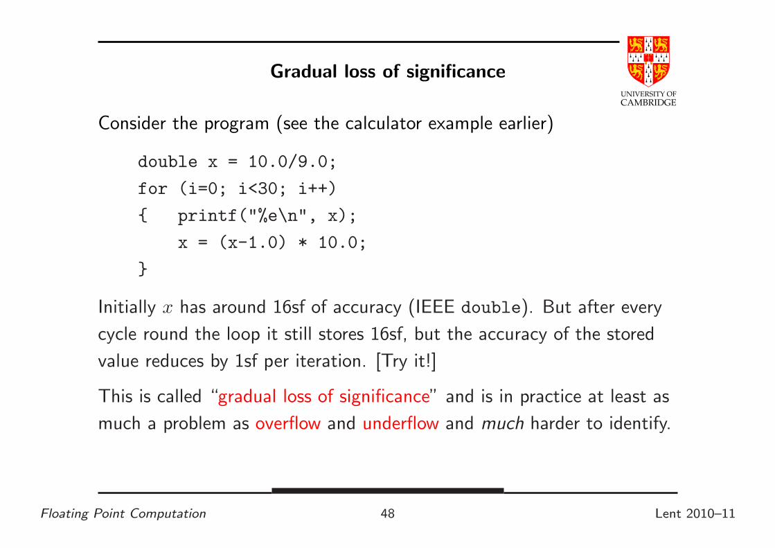
Gradual loss of significance
Consider the program (see the calculator example earlier)
double x = 10.0/9.0;
for (i=0; i<30; i++)
{ printf("%e\n", x);
x = (x-1.0) * 10.0;
}
Initially x has around 16sf of accuracy (IEEE double). But after every
cycle round the loop it still stores 16sf, but the accuracy of the stored
value reduces by 1sf per iteration. [Try it!]
This is called “gradual loss of significance” and is in practice at least as
much a problem as overflow and underflow and much harder to identify.
Floating Point Computation 48 Lent 2010–11

UNIVERSITY OF
CAMBRIDGE
Output
1.111111e+00
1.111111e+00
1.111111e+00
1.111111e+00
1.111111e+00
1.111111e+00
1.111111e+00
1.111111e+00
1.111111e+00
1.111111e+00
1.111112e+00
1.111116e+00
1.111160e+00
1.111605e+00
1.116045e+00
1.160454e+00
1.604544e+00 [≈16sf]
6.045436e+00
5.045436e+01
4.945436e+02
4.935436e+03
4.934436e+04
4.934336e+05
4.934326e+06
4.934325e+07
4.934325e+08
4.934325e+09
4.934325e+10
4.934325e+11
4.934325e+12
Note that maths says every number is in the range [1,10)!
Floating Point Computation 49 Lent 2010–11

UNIVERSITY OF
CAMBRIDGE
Machine Epsilon
Machine epsilon is defined as the difference between 1.0 and the smallest
representable number which is greater than one, i.e. 2−23 in single
precision, and 2−52 in double (in both cases β−(p−1)). ISO 9899 C says:
“the difference between 1 and the least value greater than 1
that is representable in the given floating point type”
I.e. machine epsilon is 1 ulp for the representation of 1.0.
For IEEE arithmetic, the C library <float.h> defines
#define FLT_EPSILON 1.19209290e-7F
#define DBL_EPSILON 2.2204460492503131e-16
Floating Point Computation 50 Lent 2010–11

UNIVERSITY OF
CAMBRIDGE
Machine Epsilon (2)
Machine epsilon is useful as it gives an upper bound on the relative error
caused by getting a floating point number wrong by 1 ulp, and is
therefore useful for expressing errors independent of floating point size.
(The relative error caused by being wrong by 1 ulp can be up to 50%
smaller than this, consider 1.5 or 1.9999.)
Floating point (β = 2, p = 3) numbers: macheps=0.25
0.0
· · · 6
0.25
6666
0.5
60.625
6
0.75
60.875
6
1.0
-� 61.25
6
1.5
61.75
6
2.0
62.5
6
3.0
Floating Point Computation 51 Lent 2010–11
UNIVERSITY OF
CAMBRIDGE
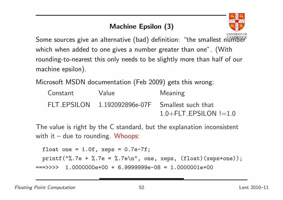
Machine Epsilon (3)
Some sources give an alternative (bad) definition: “the smallest number
which when added to one gives a number greater than one”. (With
rounding-to-nearest this only needs to be slightly more than half of our
machine epsilon).
Microsoft MSDN documentation (Feb 2009) gets this wrong:
Constant Value Meaning
FLT EPSILON 1.192092896e-07F Smallest such that
1.0+FLT EPSILON !=1.0
The value is right by the C standard, but the explanation inconsistent
with it – due to rounding. Whoops:
float one = 1.0f, xeps = 0.7e-7f;
printf("%.7e + %.7e = %.7e\n", one, xeps, (float)(xeps+one));
===>>>> 1.0000000e+00 + 6.9999999e-08 = 1.0000001e+00
Floating Point Computation 52 Lent 2010–11
UNIVERSITY OF
CAMBRIDGE
Machine Epsilon (4)
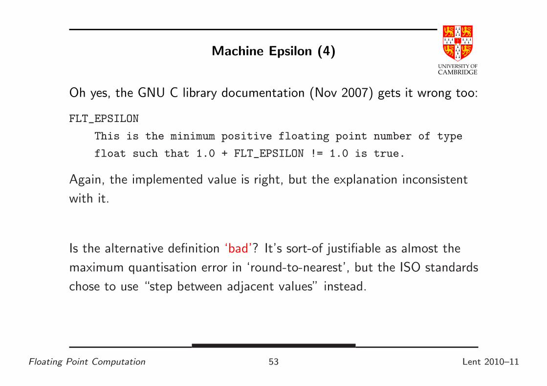
Oh yes, the GNU C library documentation (Nov 2007) gets it wrong too:
FLT_EPSILON
This is the minimum positive floating point number of type
float such that 1.0 + FLT_EPSILON != 1.0 is true.
Again, the implemented value is right, but the explanation inconsistent
with it.
Is the alternative definition ‘bad’? It’s sort-of justifiable as almost the
maximum quantisation error in ‘round-to-nearest’, but the ISO standards
chose to use “step between adjacent values” instead.
Floating Point Computation 53 Lent 2010–11

UNIVERSITY OF
CAMBRIDGE
Machine Epsilon (5) – Negative Epsilon
We defined machine epsilon as the difference between 1.0 and the
smallest representable number which is greater than one.
What about the difference between 1.0 and the greatest representable
number which is smaller than one?
In IEEE arithmetic this is exactly 50% of machine epsilon.
Why? Witching-hour effect. Let’s illustrate with precision of 5 binary
places (4 stored). One is 20 × 1.0000, the next smallest number is
20 × 0.111111111 . . . truncated to fit. But when we write this
normalised it is 2−1 × 1.1111 and so its ulp represents only half as much
as the ulp in 20 × 1.0001.
Floating Point Computation 54 Lent 2010–11
UNIVERSITY OF
CAMBRIDGE
Revisiting sin 1e40
The answer given by xcalc earlier is totally bogus. Why?
1040 is stored (like all numbers) with a relative error of around machine
epsilon. (So changing the stored value by 1 ulp results in an absolute
error of around 1040 × machine epsilon.) Even for double (16sf), this
absolute error of representation is around 1024. But the sin function
cycles every 2π. So we can’t even represent which of many billions of
cycles of sine that 1040 should be in, let alone whether it has any
sig.figs.!
On a decimal calculator 1040 is stored accurately, but I would need π to
50sf to have 10sf left when I have range-reduced 1040 into the range
[0, π/2]. So, who can calculate sin 1e40? Volunteers?
Floating Point Computation 55 Lent 2010–11
UNIVERSITY OF
CAMBRIDGE
Part 4
Simple maths, simple programs
Floating Point Computation 56 Lent 2010–11

UNIVERSITY OF
CAMBRIDGE
Non-iterative programs
Iterative programs need additional techniques, because the program may
be locally sensible, but a small representation or rounding error can
slowly grow over many iterations so as to render the result useless.
So let’s first consider a program with a fixed number of operations:
x =−b ±
√b2 − 4ac
2a
Or in C/Java:
double root1(double a, double b, double c)
{ return (-b + sqrt(b*b - 4*a*c))/(2*a); }
double root2(double a, double b, double c)
{ return (-b - sqrt(b*b - 4*a*c))/(2*a); }
What could be wrong with this so-simple code?
Floating Point Computation 57 Lent 2010–11

UNIVERSITY OF
CAMBRIDGE
Solving a quadratic
Let’s try to make sure the relative error is small.
Most operations in x = −b±√
b2−4ac2a
are multiply, divide, sqrt—these add
little to relative error (see earlier): unary negation is harmless too.
But there are two additions/subtractions: b2 − 4ac and −b ±√
(· · ·).Cancellation in the former (b2 ≈ 4ac) is not too troublesome (why?),
but consider what happens if b2 ≫ 4ac. This causes the latter ± to be
problematic for one of the two roots.
Just consider b > 0 for now, then the problem root (the smaller one in
magnitude) is−b +
√b2 − 4ac
2a.
Floating Point Computation 58 Lent 2010–11

UNIVERSITY OF
CAMBRIDGE
Getting the small root right
x =−b +
√b2 − 4ac
2a
=−b +
√b2 − 4ac
2a.−b −
√b2 − 4ac
−b −√
b2 − 4ac
=−2c
b +√
b2 − 4ac
These are all equal in maths, but the final expression computes the little
root much more accurately (no cancellation if b > 0).
But keep the big root calculation as
x =−b −
√b2 − 4ac
2a
Need to do a bit more (i.e. opposite) work if b < 0
Floating Point Computation 59 Lent 2010–11

UNIVERSITY OF
CAMBRIDGE
Illustration—quadrat float.c
1 x^2 + -3 x + 2 =>
root1 2.000000e+00 (or 2.000000e+00 double)
1 x^2 + 10 x + 1 =>
root1 -1.010203e-01 (or -1.010205e-01 double)
1 x^2 + 100 x + 1 =>
root1 -1.000214e-02 (or -1.000100e-02 double)
1 x^2 + 1000 x + 1 =>
root1 -1.007080e-03 (or -1.000001e-03 double)
1 x^2 + 10000 x + 1 =>
root1 0.000000e+00 (or -1.000000e-04 double)
root2 -1.000000e+04 (or -1.000000e+04 double)
Floating Point Computation 60 Lent 2010–11
UNIVERSITY OF
CAMBRIDGE
Summing a Finite Series
We’ve already seen (a + b) + c 6= a + (b + c) in general. So what’s the
best way to do (say)n∑
i=0
1
i + π?
Of course, while this formula mathematically sums to infinity for n = ∞,
if we calculate, using float
1
0 + π+
1
1 + π+ · · · + 1
i + π+ · · ·
until the sum stops growing we get 13.8492260 after 2097150 terms.
But is this correct? Is it the only answer?
[See sumfwdback.c on the course website for a program.]
Floating Point Computation 61 Lent 2010–11

UNIVERSITY OF
CAMBRIDGE
Summing a Finite Series (2)
Previous slide said: using float with N = 2097150 we got
1
0 + π+
1
1 + π+ · · · + 1
N + π= 13.8492260
But, by contrast
1
N + π+ · · · + 1
1 + π+
1
0 + π= 13.5784464
Using double precision (64-bit floating point) we get:
• forward: 13.5788777897524611
• backward: 13.5788777897519921
So the backwards one seems better. But why?
Floating Point Computation 62 Lent 2010–11

UNIVERSITY OF
CAMBRIDGE
Summing a Finite Series (3)
When adding a + b + c it is generally more accurate to sum the smaller
two values and then add the third. Compare (14 + 14) + 250 = 280 with
(250 + 14) + 14 = 270 when using 2sf decimal – and carefully note
where rounding happens.
So summing backwards is best for the (decreasing) series in the previous
slide.
Floating Point Computation 63 Lent 2010–11
UNIVERSITY OF
CAMBRIDGE
Summing a Finite Series (4)
General tips for an accurate result:
• Sum starting from smallest
• Even better, take the two smallest elements and replace them with
their sum (repeat until just one left).
• If some numbers are negative, add them with similar-magnitude
positive ones first (this reduces their magnitude without losing
accuracy).
Floating Point Computation 64 Lent 2010–11
UNIVERSITY OF
CAMBRIDGE
Summing a Finite Series (5)
A neat general algorithm (non-examinable) is Kahan’s summation
algorithm:
http://en.wikipedia.org/wiki/Kahan_summation_algorithm
This uses a second variable which approximates the error in the previous
step which can then be used to compensate in the next step.
For the example in the notes, even using single precision it gives:
• Kahan forward: 13.5788774
• Kahan backward: 13.5788774
which is within one ulp of the double sum 13.57887778975. . .
A chatty article on summing can be found in Dr Dobb’s Journal:
http://www.ddj.com/cpp/184403224
Floating Point Computation 65 Lent 2010–11

UNIVERSITY OF
CAMBRIDGE
Part 5
Infinitary/limiting computations
Floating Point Computation 66 Lent 2010–11

UNIVERSITY OF
CAMBRIDGE
Rounding versus Truncation Error
Many mathematical processes are infinitary, e.g. limit-taking (including
differentiation, integration, infinite series), and iteration towards a
solution.
There are now two logically distinct forms of error in our calculations
Rounding error the error we get by using finite arithmetic during a
computation. [We’ve talked about this exclusively until now.]
Truncation error (a.k.a. discretisation error) the error we get by
stopping an infinitary process after a finite point. [This is new]
Note the general antagonism: the finer the mathematical approximation
the more operations which need to be done, and hence the worse the
accumulated error. Need to compromise, or really clever algorithms
(beyond this course).
Floating Point Computation 67 Lent 2010–11
UNIVERSITY OF
CAMBRIDGE
Illustration—differentiation
Suppose we have a nice civilised function f (we’re not even going to look
at malicious ones). By civilised I mean smooth (derivatives exist) and
f(x), f ′(x) and f ′′(x) are around 1 (i.e. between, say, 0.1 and 10 rather
than 1015 or 10−15 or, even worse, 0.0). Let’s suppose we want to
calculate an approximation to f ′(x) at x = 1.0 given only the code for f .
Mathematically, we define
f ′(x) = limh→0
(
f(x + h) − f(x)
h
)
So, we just calculate (f(x + h) − f(x))/h, don’t we?
Well, just how do we choose h? Does it matter?
Floating Point Computation 68 Lent 2010–11
UNIVERSITY OF
CAMBRIDGE
Illustration—differentiation (2)
The maths for f ′(x) says take the limit as h tends to zero. But if h is
smaller than machine epsilon (2−23 for float and 2−52 for double)
then, for x about 1, x + h will compute to the same value as x. So
f(x + h) − f(x) will evaluate to zero!
There’s a more subtle point too, if h is small then f(x + h) − f(x) will
produce lots of cancelling (e.g. 1.259− 1.257) hence a high relative error
(few sig.figs. in the result).
‘Rounding error.’
But if h is too big, we also lose: e.g. dx2/dx at 1 should be 2, but
taking h = 1 we get (22 − 12)/1 = 3.0. Again a high relative error (few
sig.figs. in the result).
‘Truncation error.’
Floating Point Computation 69 Lent 2010–11

UNIVERSITY OF
CAMBRIDGE
Illustration—differentiation (3)
Answer: the two errors vary oppositely w.r.t. h, so compromise by
making the two errors of the same order to minimise their total effect.
The truncation error can be calculated by Taylor:
f(x + h) = f(x) + hf ′(x) + h2f ′′(x)/2 + O(h3)
So the truncation error in the formula is approximately hf ′′(x)/2 (check
it yourself), i.e. about h given the assumption on f ′′ being around 1.
Floating Point Computation 70 Lent 2010–11

UNIVERSITY OF
CAMBRIDGE
Illustration—differentiation (4)
For rounding error use Taylor again, and allow a minimal error of
macheps to creep into f and get (remember we’re also assuming f(x)
and f ′(x) is around 1, and we’ll write macheps for machine epsilon):
(f(x + h) − f(x))/h = (f(x) + hf ′(x) ± macheps − f(x))/h
= 1 ± macheps/h
So the rounding error is macheps/h.
Equating rounding and truncation errors gives h = macheps/h, i.e.
h =√
macheps (around 3.10−4 for single precision and 10−8 for double).
[See diff float.c for a program to verify this—note the truncation
error is fairly predictable, but the rounding error is “anywhere in an
error-bar”]
Floating Point Computation 71 Lent 2010–11
UNIVERSITY OF
CAMBRIDGE
Illustration—differentiation (5)
The Standard ML example in Wikipedia quotes an alternative form of
differentiation:
(f(x + h) − f(x − h))/2h
But, applying Taylor’s approximation as above to this function gives a
truncation error of
h2f ′′′(x)/3!
The rounding error remains at about macheps/h. Now, equating
truncation and rounding error as above means that say h = 3√
macheps
is a good choice for h.
Entertainingly, until 2007, the article mistakenly said “square root”
(. . . recalling the result but applying it to the wrong problem)!
Floating Point Computation 72 Lent 2010–11
UNIVERSITY OF
CAMBRIDGE
Illustration—differentiation (6)
There is a serious point in discussing the two methods of differentiation
as it illustrates an important concept.
Usually when finitely approximating some limiting process there is a
number like h which is small, or a number n which is large. Sometimes
both logically occur (with h = 1/n)
∫ 1
0
f(x) ≈(
n∑
i=1
f(i/n)
)
/n
Often there are multiple algorithms which mathematically have the same
limit (see the two differentiation examples above), but which have
different rates of approaching the limit (in addition to possibly different
rounding error accumulation which we’re not considering at the
moment).
Floating Point Computation 73 Lent 2010–11
UNIVERSITY OF
CAMBRIDGE
Illustration—differentiation (7)
The way in which truncation error is affected by reducing h (or
increasing n) is called the order of the algorithm (or more precisely the
mathematics on which the algorithm is based).
For example, (f(x + h) − f(x))/h is a first-order method of
approximating derivatives of smooth function (halving h halves the
truncation error.)
On the other hand, (f(x + h) − f(x − h))/2h is a second-order
method—halving h divides the truncation error by 4.
A large amount of effort over the past 50 years has been invested in
finding techniques which give higher-order methods so a relatively large
h can be used without incurring excessive truncation error (and
incidentally, this often reduce rounding error too).
Don’t assume you can outguess the experts.
Floating Point Computation 74 Lent 2010–11
UNIVERSITY OF
CAMBRIDGE
Iteration and when to stop
Consider the “golden ratio” φ = (1 +√
5)/2 ≈ 1.618. It satisfies
φ2 = φ + 1.
So, supposing we didn’t know how to solve quadratics, we could re-write
this as “φ is the solution of x =√
x + 1”.
Numerically, we could start with x0 = 2 (say) and then set
xn+1 =√
xn + 1, and watch how the xn evolve (an iteration) . . .
Floating Point Computation 75 Lent 2010–11

UNIVERSITY OF
CAMBRIDGE
Golden ratio iteration
i x err err/prev.err
1 1.7320508075688772 1.1402e-01
2 1.6528916502810695 3.4858e-02 3.0572e-01
3 1.6287699807772333 1.0736e-02 3.0800e-01
4 1.6213481984993949 3.3142e-03 3.0870e-01
5 1.6190578119694785 1.0238e-03 3.0892e-01
. . .
26 1.6180339887499147 1.9762e-14 3.0690e-01
27 1.6180339887499009 5.9952e-15 3.0337e-01
28 1.6180339887498967 1.7764e-15 2.9630e-01
29 1.6180339887498953 4.4409e-16 2.5000e-01
30 1.6180339887498949 0.0000e+00 0.0000e+00
31 1.6180339887498949 0.0000e+00 nan
32 1.6180339887498949 0.0000e+00 nan
Floating Point Computation 76 Lent 2010–11
UNIVERSITY OF
CAMBRIDGE
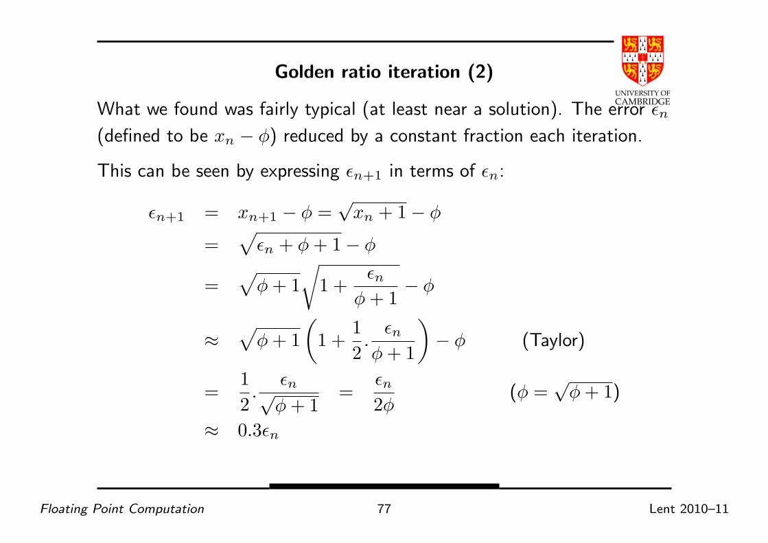
Golden ratio iteration (2)
What we found was fairly typical (at least near a solution). The error ǫn
(defined to be xn − φ) reduced by a constant fraction each iteration.
This can be seen by expressing ǫn+1 in terms of ǫn:
ǫn+1 = xn+1 − φ =√
xn + 1 − φ
=√
ǫn + φ + 1 − φ
=√
φ + 1
√
1 +ǫn
φ + 1− φ
≈√
φ + 1
(
1 +1
2.
ǫn
φ + 1
)
− φ (Taylor)
=1
2.
ǫn√φ + 1
=ǫn
2φ(φ =
√φ + 1)
≈ 0.3ǫn
Floating Point Computation 77 Lent 2010–11

UNIVERSITY OF
CAMBRIDGE
Golden ratio iteration (3)
The termination criterion: here we were lucky. We can show
mathematically that if xn > φ then φ ≤ xn+1 ≤ xn, so a suitable
termination criterion is xn+1 ≥ xn.
In general we don’t have such a nice property, so we terminate when
|xn+1 − xn| < δ for some prescribed threshold δ.
Nomenclature:
When ǫn+1 = kǫn we say that the iteration exhibits “first order
convergence”. For the iteration xn+1 = f(xn) then k is merely f ′(σ)
where σ is the solution of σ = f(σ) to which iteration is converging.
For the earlier iteration this is 1/2φ.
Floating Point Computation 78 Lent 2010–11

UNIVERSITY OF
CAMBRIDGE
Golden ratio iteration (4)
What if, instead of writing φ2 = φ + 1 as the iteration xn+1 =√
xn + 1,
we had instead written it as xn+1 = x2n − 1?
Putting g(x) = x2 − 1, we have g′(φ) = 2φ ≈ 3.236. Does this mean
that the error increases: ǫn+1 ≈ 3.236ǫn?
Floating Point Computation 79 Lent 2010–11

UNIVERSITY OF
CAMBRIDGE
Golden ratio iteration (5)
Yes! This is a bad iteration (magnifies errors).
Putting x0 = φ + 10−16 computes xi as below:
i x err err/prev.err
1 1.6180339887498951 2.2204e-16
2 1.6180339887498958 8.8818e-16 4.0000e+00
3 1.6180339887498978 2.8866e-15 3.2500e+00
4 1.6180339887499045 9.5479e-15 3.3077e+00
5 1.6180339887499260 3.1086e-14 3.2558e+00
6 1.6180339887499957 1.0081e-13 3.2429e+00
7 1.6180339887502213 3.2641e-13 3.2379e+00
. . .
32 3.9828994989829472 2.3649e+00 3.8503e+00
33 14.8634884189986121 1.3245e+01 5.6009e+00
34 219.9232879817058688 2.1831e+02 1.6482e+01
Floating Point Computation 80 Lent 2010–11

UNIVERSITY OF
CAMBRIDGE
Iteration issues
• Choose your iteration well.
• Determine a termination criterion.
For real-world equations (possibly in multi-dimensional space) neither of
these are easy and it may well be best to consult an expert!
Floating Point Computation 81 Lent 2010–11
UNIVERSITY OF
CAMBRIDGE
Newton–Raphson
Given an equation of the form f(x) = 0 then the Newton-Raphson
iteration improves an initial estimate x0 of the root by repeatedly setting
xn+1 = xn − f(xn)
f ′(xn)
See http://en.wikipedia.org/wiki/Newton’s_method for
geometrical intuition – intersection of a tangent with the x-axis.
Floating Point Computation 82 Lent 2010–11
UNIVERSITY OF
CAMBRIDGE
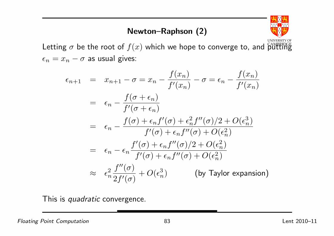
Newton–Raphson (2)
Letting σ be the root of f(x) which we hope to converge to, and putting
ǫn = xn − σ as usual gives:
ǫn+1 = xn+1 − σ = xn − f(xn)
f ′(xn)− σ = ǫn − f(xn)
f ′(xn)
= ǫn − f(σ + ǫn)
f ′(σ + ǫn)
= ǫn − f(σ) + ǫnf ′(σ) + ǫ2nf ′′(σ)/2 + O(ǫ3n)
f ′(σ) + ǫnf ′′(σ) + O(ǫ2n)
= ǫn − ǫn
f ′(σ) + ǫnf ′′(σ)/2 + O(ǫ2n)
f ′(σ) + ǫnf ′′(σ) + O(ǫ2n)
≈ ǫ2nf ′′(σ)
2f ′(σ)+ O(ǫ3n) (by Taylor expansion)
This is quadratic convergence.
Floating Point Computation 83 Lent 2010–11
UNIVERSITY OF
CAMBRIDGE
Newton–Raphson (3)
Pros and Cons:
• Quadratic convergence means that the number of decimal (or
binary) digits doubles every iteration
• Problems if we start with |f ′(x0)| being small
• (even possibility of looping)
• Behaves badly for multiple roots
Floating Point Computation 84 Lent 2010–11
UNIVERSITY OF
CAMBRIDGE
Summing a Taylor series
Various problems can be solved by summing a Taylor series, e.g.
sin(x) = x − x3
3!+
x5
5!− x7
7!+ · · ·
Mathematically, this is as nice as you can get—it unconditionally
converges everywhere. However, computationally things are trickier.
Floating Point Computation 85 Lent 2010–11

UNIVERSITY OF
CAMBRIDGE
Summing a Taylor series (2)
Trickinesses:
• How many terms? [stopping early gives truncation error]
• Large cancelling intermediate terms can cause loss of precision
[hence rounding error]
e.g. the biggest term in sin(15) [radians] is over -334864 giving (in
single precision float) a result with only 1 sig.fig.
[See sinseries float.c.]
Floating Point Computation 86 Lent 2010–11

UNIVERSITY OF
CAMBRIDGE
Summing a Taylor series (3)
Solution:
• Do range reduction—use identities to reduce the argument to the
range [0, π/2] or even [0, π/4]. However: this might need a lot of
work to make sin(1040) or sin(2100) work (since we need π to a
large accuracy).
• Now we can choose a fixed number of iterations and unroll the loop
(conditional branches can be slow in pipelined architectures),
because we’re now just evaluating a polynomial.
Floating Point Computation 87 Lent 2010–11

UNIVERSITY OF
CAMBRIDGE
Summing a Taylor series (4)
If we sum a series up to terms in xn, i.e. we compute
i=n∑
i=0
aixi
then the first missing term will by in xn+1 (or xn+2 for sin(x)). This will
be the dominant error term (i.e. most of the truncation error), at least
for small x.
However, xn+1 is unpleasant – it is very very small near the origin but its
maximum near the ends of the input range can be thousands of times
bigger.
Floating Point Computation 88 Lent 2010–11

UNIVERSITY OF
CAMBRIDGE
Summing a Taylor series (5)
Using Chebyshev polynomials [non-examinable] the total error is
re-distributed from the edges of the input range to throughout the input
range and at the same time the maximum absolute error is reduced by
orders of magnitude.
We calculate a new polynomial
i=n∑
i=0
a′ix
i
where a′i is a small adjustment of ai above. This is called ‘power series
economisation’ because it can cut the number of terms (and hence the
execution time) needed for a given Taylor series to a produce given
accuracy.
Floating Point Computation 89 Lent 2010–11
UNIVERSITY OF
CAMBRIDGE
Summing a Taylor series (6)
See also the Matlab file poly.m from the course web-site about how
careless calculation of polynomials can cause noise from rounding error.
(Insert graph here.)
Floating Point Computation 90 Lent 2010–11

UNIVERSITY OF
CAMBRIDGE
Why fuss about Taylor . . .
. . . and not (say) integration or similar?
It’s a general metaphor—in six lectures I can’t tell you 50 years of maths
and really clever tricks (and there is comparable technology for
integration, differential equations etc.!). [Remember when the CS
Diploma here started in 1953 almost all of the course material would
have been on such numerical programming; in earlier days this course
would have been called an introduction to “Numerical Analysis”.]
But I can warn you that if you need precision, or speed, or just to show
your algorithm is producing a mathematically justifiable answer then you
may (and will probably if the problem is non-trivial) need to consult an
expert, or buy in a package with certified performance (e.g. NAGLIB,
Matlab, Maple, Mathematica, REDUCE . . . ).
Floating Point Computation 91 Lent 2010–11
UNIVERSITY OF
CAMBRIDGE
How accurate do you want to be?
If you want to implement (say) sin(x)
double sin(double x)
with the same rules as the IEEE basic operations (the result must be the
nearest IEEE representable number to the mathematical result when
treating the argument as precise) then this can require a truly Herculean
effort. (You’ll certainly need to do much of its internal computation in
higher precision than its result.)
On the other hand, if you just want a function which has known error
properties (e.g. correct apart from the last 2 sig.figs.) and you may not
mind oddities (e.g. your implementation of sine not being monotonic in
the first quadrant) then the techniques here suffice.
Floating Point Computation 92 Lent 2010–11
UNIVERSITY OF
CAMBRIDGE
How accurate do you want to be? (2)
Sometimes, e.g. writing a video game, profiling may show that the time
taken in some floating point routine like sqrt may be slowing down the
number of frames per second below what you would like, Then, and only
then, you could consider alternatives, e.g. rewriting your code to avoid
using sqrt or replacing calls to the system provided (perhaps accurate
and slow) routine with calls to a faster but less accurate one.
Floating Point Computation 93 Lent 2010–11
UNIVERSITY OF
CAMBRIDGE
How accurate do you want to be? (3)
Chris Lomont
(http://www.lomont.org/Math/Papers/2003/InvSqrt.pdf) writes
[fun, not examinable]:
“Computing reciprocal square roots is necessary in many
applications, such as vector normalization in video games.
Often, some loss of precision is acceptable for a large increase in
speed.”
He wanted to get the frame rate up in a video game and considers:
Floating Point Computation 94 Lent 2010–11
UNIVERSITY OF
CAMBRIDGE
How accurate do you want to be? (4)
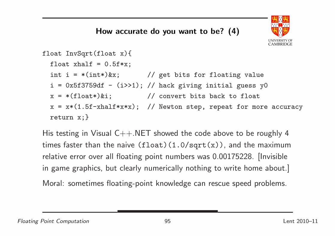
float InvSqrt(float x){
float xhalf = 0.5f*x;
int i = *(int*)&x; // get bits for floating value
i = 0x5f3759df - (i>>1); // hack giving initial guess y0
x = *(float*)&i; // convert bits back to float
x = x*(1.5f-xhalf*x*x); // Newton step, repeat for more accuracy
return x;}
His testing in Visual C++.NET showed the code above to be roughly 4
times faster than the naive (float)(1.0/sqrt(x)), and the maximum
relative error over all floating point numbers was 0.00175228. [Invisible
in game graphics, but clearly numerically nothing to write home about.]
Moral: sometimes floating-point knowledge can rescue speed problems.
Floating Point Computation 95 Lent 2010–11
UNIVERSITY OF
CAMBRIDGE
Why do I use float so much . . .
. . . and is it recommended? [No!]
I use single precision because the maths uses smaller numbers (223
instead of 252) and so I can use double precision for comparison—I can
also use smaller programs/numbers to exhibit the flaws inherent in
floating point. But for most practical problems I would recommend you
use double almost exclusively.
Why: smaller errors, often no or little speed penalty.
What’s the exception: floating point arrays where the size matters and
where (i) the accuracy lost in the storing/reloading process is
manageable and analysable and (ii) the reduced exponent range is not a
problem.
Floating Point Computation 96 Lent 2010–11
UNIVERSITY OF
CAMBRIDGE
Notes for C users
• float is very much a second class type like char and short.
• Constants 1.1 are type double unless you ask 1.1f.
• floats are implicitly converted to doubles at various points (e.g.
for ‘vararg’ functions like printf).
• The ISO/ANSI C standard says that a computation involving only
floats may be done at type double, so f and g in
float f(float x, float y) { return (x+y)+1.0f; }
float g(float x, float y) { float t = (x+y); return t+1.0f; }
may give different results.
So: use double rather than float whenever possible for language as
well as numerical reasons. (Large arrays are really the only thing worth
discussing.)
Floating Point Computation 97 Lent 2010–11
UNIVERSITY OF
CAMBRIDGE
Part 6
Some statistical remarks
Floating Point Computation 98 Lent 2010–11
UNIVERSITY OF
CAMBRIDGE
How do errors add up in practice?
During a computation rounding errors will accumulate, and in the worst
case will often approach the error bounds we have calculated.
However, remember that IEEE rounding was carefully arranged to be
statistically unbiased—so for many programs (and inputs) the errors
from each operation behave more like independent random errors of
mean zero and standard deviation σ.
So, often one finds a k-operations program produces errors of around
macheps.√
k rather than macheps.k/2 (because independent random
variables’ variances sum).
BEWARE: just because the errors tend to cancel for some inputs does
not mean that they will do so for all! Trust bounds rather than
experiment.
Floating Point Computation 99 Lent 2010–11
UNIVERSITY OF
CAMBRIDGE
Part 7
Some nastier issues
Floating Point Computation 100 Lent 2010–11
UNIVERSITY OF
CAMBRIDGE
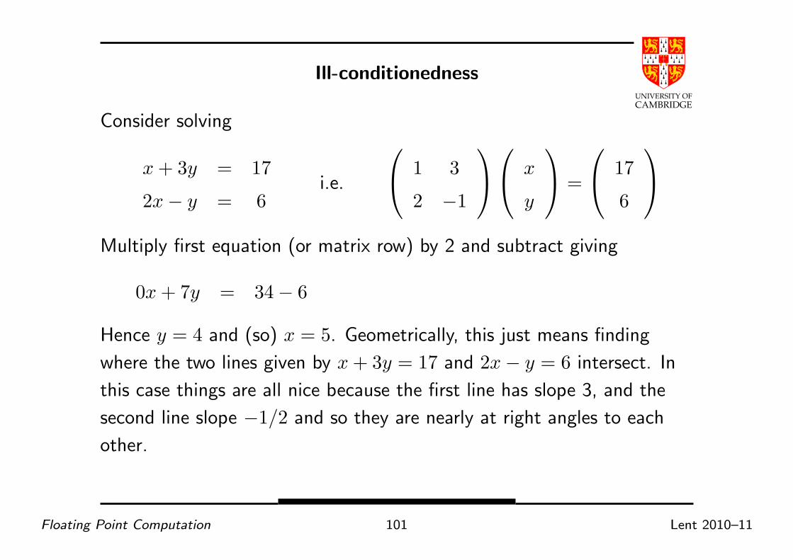
Ill-conditionedness
Consider solving
x + 3y = 17
2x − y = 6i.e.
1 3
2 −1
x
y
=
17
6
Multiply first equation (or matrix row) by 2 and subtract giving
0x + 7y = 34 − 6
Hence y = 4 and (so) x = 5. Geometrically, this just means finding
where the two lines given by x + 3y = 17 and 2x − y = 6 intersect. In
this case things are all nice because the first line has slope 3, and the
second line slope −1/2 and so they are nearly at right angles to each
other.
Floating Point Computation 101 Lent 2010–11

UNIVERSITY OF
CAMBRIDGE
Ill-conditionedness (2)
Remember, in general, that if
a b
c d
x
y
=
p
q
Then
x
y
=
a b
c d
−1
p
q
=1
ad − bc
d −b
−c a
p
q
Oh, and look, there’s a numerically-suspect calculation of ad − bc !
So there are problems if ad − bc is small (not absolutely small, consider
a = b = d = 10−10, c = −10−10, but relatively small e.g. w.r.t.
a2 + bc + c2 + d2). The lines then are nearly parallel.
Floating Point Computation 102 Lent 2010–11

UNIVERSITY OF
CAMBRIDGE
Ill-conditionedness (3)
Here’s how to make a nasty case based on the Fibonacci numbers
f1 = f2 = 1, fn = fn−1 + fn−1 for n > 2
which means that taking a = fn, b = fn−1, c = fn−2, d = fn−3 gives
ad − bc = 1 (and this ‘1’ only looks (absolute error) harmless, but it is
nasty in relative terms). So,
17711 10946
6765 4181
−1
=
4181 −10946
−6765 17711
and this all looks so harmless, but..
Floating Point Computation 103 Lent 2010–11

UNIVERSITY OF
CAMBRIDGE
Ill-conditionedness (4)
Consider the harmless-looking
1.7711 1.0946
0.6765 0.4181
x
y
=
p
q
Solving we get
x
y
=
41810000 −109460000
−67650000 177110000
p
q
which no longer looks so harmless—as a change in p or q by a very small
absolute error gives a huge absolute error in x and y. And a change of
a,b,c or d by one in the last decimal place changes any of the numbers in
its inverse by a factor of at least 2. (Consider this geometrically.)
Floating Point Computation 104 Lent 2010–11
UNIVERSITY OF
CAMBRIDGE
Ill-conditionedness (5)
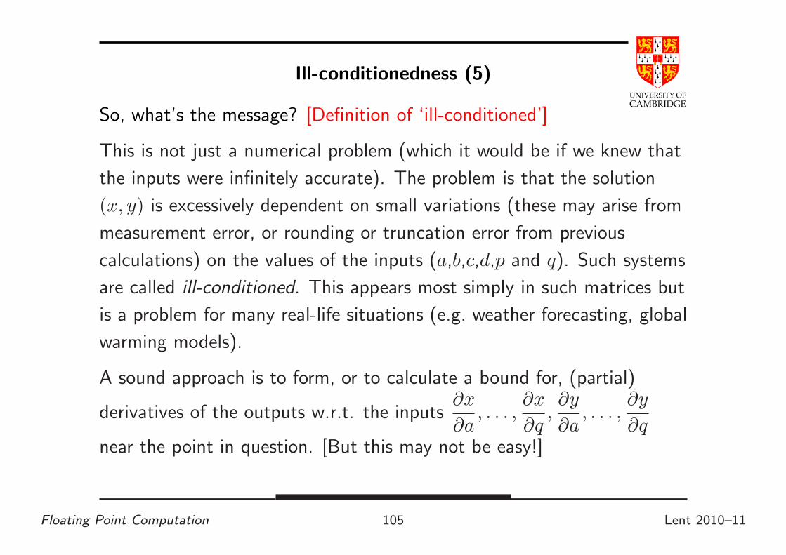
So, what’s the message? [Definition of ‘ill-conditioned’]
This is not just a numerical problem (which it would be if we knew that
the inputs were infinitely accurate). The problem is that the solution
(x, y) is excessively dependent on small variations (these may arise from
measurement error, or rounding or truncation error from previous
calculations) on the values of the inputs (a,b,c,d,p and q). Such systems
are called ill-conditioned. This appears most simply in such matrices but
is a problem for many real-life situations (e.g. weather forecasting, global
warming models).
A sound approach is to form, or to calculate a bound for, (partial)
derivatives of the outputs w.r.t. the inputs∂x
∂a, . . . ,
∂x
∂q,∂y
∂a, . . . ,
∂y
∂qnear the point in question. [But this may not be easy!]
Floating Point Computation 105 Lent 2010–11
UNIVERSITY OF
CAMBRIDGE
Ill-conditionedness (6)
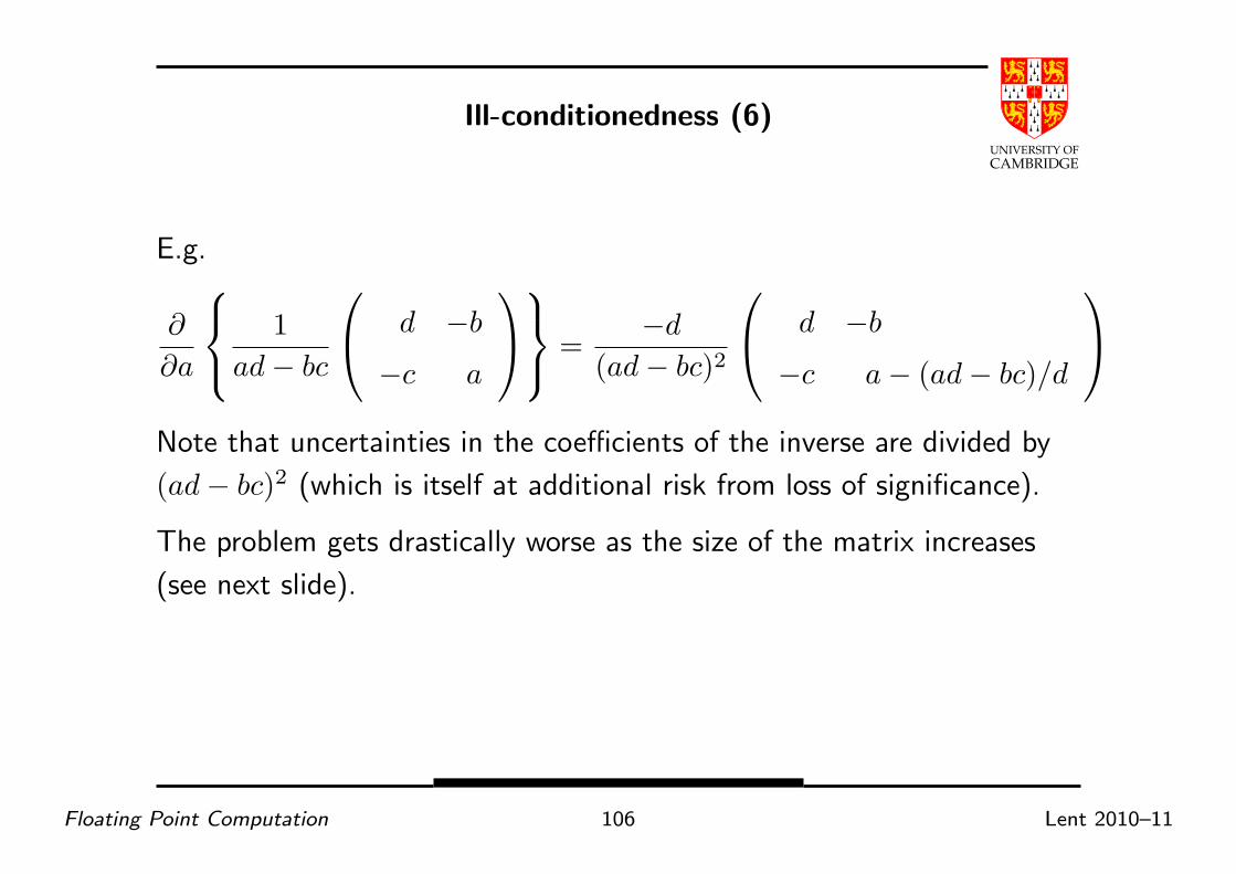
E.g.
∂
∂a
1
ad − bc
d −b
−c a
=−d
(ad − bc)2
d −b
−c a − (ad − bc)/d
Note that uncertainties in the coefficients of the inverse are divided by
(ad − bc)2 (which is itself at additional risk from loss of significance).
The problem gets drastically worse as the size of the matrix increases
(see next slide).
Floating Point Computation 106 Lent 2010–11
UNIVERSITY OF
CAMBRIDGE
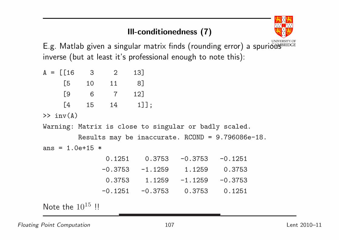
Ill-conditionedness (7)
E.g. Matlab given a singular matrix finds (rounding error) a spurious
inverse (but at least it’s professional enough to note this):
A = [[16 3 2 13]
[5 10 11 8]
[9 6 7 12]
[4 15 14 1]];
>> inv(A)
Warning: Matrix is close to singular or badly scaled.
Results may be inaccurate. RCOND = 9.796086e-18.
ans = 1.0e+15 *
0.1251 0.3753 -0.3753 -0.1251
-0.3753 -1.1259 1.1259 0.3753
0.3753 1.1259 -1.1259 -0.3753
-0.1251 -0.3753 0.3753 0.1251
Note the 1015 !!
Floating Point Computation 107 Lent 2010–11

UNIVERSITY OF
CAMBRIDGE
Ill-conditionedness (8)
There’s more theory around, but it’s worth noting one definition: the
condition number Kf (x) of a function f at point x is the ratio between
(small) relative changes of parameter x and corresponding relative
change of f(x). High numbers mean ‘ill-conditioned’ in that input errors
are magnified by f .
A general sanity principle for all maths routines/libraries/packages:
Substitute the answers back in the original problem and see to
what extent they are a real solution. [Didn’t you always get told
to do this when using a calculator at school?]
Floating Point Computation 108 Lent 2010–11

UNIVERSITY OF
CAMBRIDGE
Monte Carlo techniques and Ill-conditionedness
If formal methods are inappropriate for determining conditionedness of a
problem, then one can always resort to Monte Carlo (probabilistic)
techniques.
Take the original problem and solve.
Then take many variants of the problem, each varying the value of one
or more parameters or input variables by a few ulps or a few percent.
Solve all these.
If these all give similar solutions then the original problem is likely to be
well-conditioned. If not, then, you have at least been warned of the
instability.
Floating Point Computation 109 Lent 2010–11

UNIVERSITY OF
CAMBRIDGE
Adaptive Methods
I’m only mentioning these because they are in the syllabus, but I’m
regarding them as non-examinable this year.
Sometimes a problem is well-behaved in some regions but behaves badly
in another.
Then the best way might be to discretise the problem into small blocks
which has finer discretisation in problematic areas (for accuracy) but
larger in the rest (for speed).
Sometimes an iterative solution to a differential equation (e.g. to
∇2φ = 0) is fastest solved by solving for a coarse discretisation (mesh)
and then refining.
Both these are called “Adaptive Methods”.
Floating Point Computation 110 Lent 2010–11

UNIVERSITY OF
CAMBRIDGE
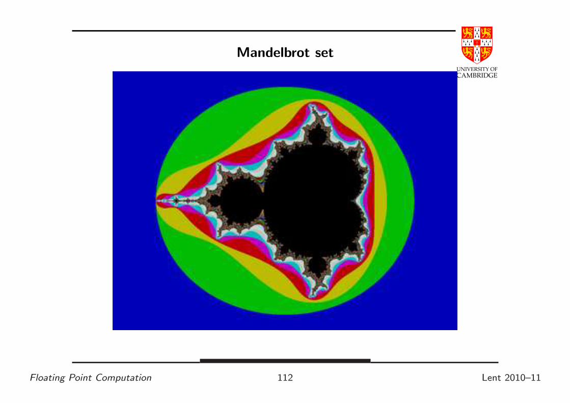
Chaotic Systems
Chaotic Systems [http://en.wikipedia.org/wiki/Chaos theory]
are just a nastier form of ill-conditionedness for which the computed
function is highly discontinuous. Typically there are arbitrarily small
input regions for which a wide range of output values occur. E.g.
• Mandelbrot set, here we count the number of iterations, k ∈ [0..∞],
of z0 = 0, zn+1 = z2n + c needed to make |zk| ≥ 2 for each point c
in the complex plane.
• Verhulst’s Logistic map xn+1 = rxn(1 − xn) with r = 4
[See http://en.wikipedia.org/wiki/Logistic map for why this
is relevant to a population of rabbits and foxes, and for r big enough
(4.0 suffices) we get chaotic behaviour. See later.]
Floating Point Computation 111 Lent 2010–11
UNIVERSITY OF
CAMBRIDGE
Mandelbrot set
Floating Point Computation 112 Lent 2010–11
UNIVERSITY OF
CAMBRIDGE
Part 8
Alternative Technologies to Floating
Point
(which avoid doing all this analysis,
but which might have other problems)
Floating Point Computation 113 Lent 2010–11

UNIVERSITY OF
CAMBRIDGE
Alternatives to IEEE arithmetic
What if, for one reason or another:
• we cannot find a way to compute a good approximation to the exact
answer of a problem, or
• we know an algorithm, but are unsure as to how errors propagate so
that the answer may well be useless.
Alternatives:
• print(random()) [well at least it’s faster than spending a long
time producing the wrong answer, and it’s intellectually honest.]
• interval arithmetic
• arbitrary precision arithmetic
• exact real arithmetic
Floating Point Computation 114 Lent 2010–11

UNIVERSITY OF
CAMBRIDGE
Interval arithmetic
The idea here is to represent a mathematical real number value with two
IEEE floating point numbers. One gives a representable number
guaranteed to be lower or equal to the mathematical value, and the other
greater or equal. Each constant or operation must preserve this property
(e.g. (aL, aU ) − (bL, bU ) = (aL − bU , aU − bL) and you might need to
mess with IEEE rounding modes to make this work; similarly 1.0 will be
represented as (1.0,1.0) but 0.1 will have distinct lower and upper limits.
This can be a neat solution. Upsides:
• naturally copes with uncertainty in input values
• IEEE arithmetic rounding modes (to +ve/-ve infinity) do much of
the work.
Floating Point Computation 115 Lent 2010–11

UNIVERSITY OF
CAMBRIDGE
Interval arithmetic (2)
This can be a neat solution to some problems. Downsides:
• Can be slow (but correctness is more important than speed)
• Some algorithms converge in practice (like Newton-Raphson) while
the computed bounds after doing the algorithm can be spuriously far
apart.
• Need a bit more work that you would expect if the range of the
denominator in a division includes 0, since the output range then
includes infinity (but it still can be seen as a single range).
• Conditions (like x < y) can be both true and false.
Floating Point Computation 116 Lent 2010–11

UNIVERSITY OF
CAMBRIDGE
Interval arithmetic (3)
[For Part IB students only]
C++ fans: this is an ideal class for you to write:
class interval
{ interval(char *) { /* constructor... */ }
static interval operator +(interval x, interval y) { ... };
};
and a bit of trickery such as #define float interval will get you
started coding easily.
Floating Point Computation 117 Lent 2010–11
UNIVERSITY OF
CAMBRIDGE
Arbitrary Precision Floating Point
Some packages allow you to set the precision on a run-by-run basis. E.g.
use 50 sig.fig. today.
For any fixed precision the same problems arise as with IEEE 32- and
64-bit arithmetic, but at a different point, so it can be worth doing this
for comparison.
Some packages even allow allow adaptive precision. Cf. lazy evaluation:
if I need e1 − e2 to 50 sig.fig. then calculate e1 and e2 to 50 sig.fig. If
these reinforce then all is OK, but if they cancel then calculate e1 and e2
to more accuracy and repeat. There’s a problem here with zero though.
Consider calculating1√2− sin(tan−1(1))
(This problem of when an algebraic expression really is exactly zero is
formally uncomputable—CST Part Ib has lectures on computability.)
Floating Point Computation 118 Lent 2010–11
UNIVERSITY OF
CAMBRIDGE
Exact Real Arithmetic
This term generally refers to better representations than digit streams
(because it is impossible to print the first digit (0 or 1) of the sum
0.333333 · · · + 0.666666 · · · without evaluating until a digit appears in
the sum which is not equal to 9).
This slide is a bit vestigial – I’d originally planned on mentioning to
Part Ib the (research-level) ideas of using (infinite sequences of linear
maps; continued fraction expansions; infinite compositions of linear
fractional transformations) but this is inappropriate to Part Ia
Floating Point Computation 119 Lent 2010–11
UNIVERSITY OF
CAMBRIDGE
Exact Real Arithmetic (2)
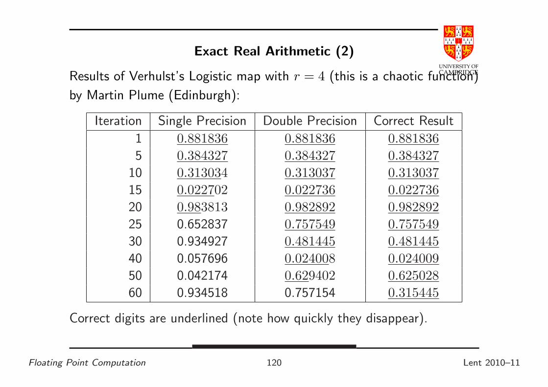
Results of Verhulst’s Logistic map with r = 4 (this is a chaotic function)
by Martin Plume (Edinburgh):
Iteration Single Precision Double Precision Correct Result
1 0.881836 0.881836 0.881836
5 0.384327 0.384327 0.384327
10 0.313034 0.313037 0.313037
15 0.022702 0.022736 0.022736
20 0.983813 0.982892 0.982892
25 0.652837 0.757549 0.757549
30 0.934927 0.481445 0.481445
40 0.057696 0.024008 0.024009
50 0.042174 0.629402 0.625028
60 0.934518 0.757154 0.315445
Correct digits are underlined (note how quickly they disappear).
Floating Point Computation 120 Lent 2010–11
UNIVERSITY OF
CAMBRIDGE
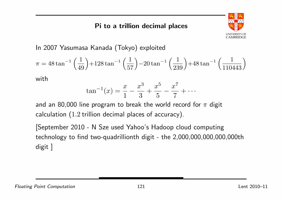
Pi to a trillion decimal places
In 2007 Yasumasa Kanada (Tokyo) exploited
π = 48 tan−1
(
1
49
)
+128 tan−1
(
1
57
)
−20 tan−1
(
1
239
)
+48 tan−1
(
1
110443
)
with
tan−1(x) =x
1− x3
3+
x5
5− x7
7+ · · ·
and an 80,000 line program to break the world record for π digit
calculation (1.2 trillion decimal places of accuracy).
[September 2010 - N Sze used Yahoo’s Hadoop cloud computing
technology to find two-quadrillionth digit - the 2,000,000,000,000,000th
digit ]
Floating Point Computation 121 Lent 2010–11

UNIVERSITY OF
CAMBRIDGE
Part 9
What have we learned?
Floating Point Computation 122 Lent 2010–11
UNIVERSITY OF
CAMBRIDGE
What have we learned?
Any floating point computation should be treated with the utmost
suspicion unless you can argue how accurate it is
. . . because . . .
here be dragons!
Floating Point Computation 123 Lent 2010–11