A Simultaneous Optimization Approach for Off-line Blending ...

A Simultaneous Optimization Approach for Off-line Blending

and Scheduling of Oil-refinery Operations

Carlos A. Mendez, Ignacio E. Grossmann Department of Chemical Engineering - Carnegie Mellon University

Pittsburgh, USA

Iiro Harjunkoski, Pousga Kaboré ABB Corporate Research Center

Ladenburg, Germany

Abstract This paper presents a novel MILP-based method that addresses the simultaneous optimization of the

off-line blending and the short-term scheduling problem in oil-refinery applications. Depending on the

problem characteristics as well as the required flexibility in the solution, the model can be based on either a

discrete or a continuous-time domain representation. In order to preserve the model’s linearity, an iterative

procedure is proposed to effectively deal with non-linear gasoline properties and variable recipes for

different product grades. Thus, the solution of a very complex MINLP formulation is replaced by a

sequential MILP approximation. Instead of predefining fixed component concentrations for products,

preferred blend recipes can be forced to apply whenever it is possible. The proposed optimization approach

is oriented towards providing an effective and integrated solution for the blending and the scheduling of

large-scale problems. In order to provide convenient solutions for all circumstances, different alternatives

for coping with infeasible problems are presented. The new method is illustrated by solving several real

world problems with very low computational requirements.

1. INTRODUCTION The main objective in oil refining is to convert a wide variety of crude oils into valuable final products

such as gasoline, jet fuel and diesel. The short-term blending and scheduling are critical aspects in this

large and complex process. The economic and operability benefits associated with obtaining better-quality

2

and less expensive blends, and at the same time making a more effective use of the available resources over

time, are numerous and significant. A wide variety of mathematical programming techniques have been

extensively used for long-term planning as well as the short-term scheduling of refinery operations.

For planning problems, most of the computational tools have been based on successive linear

programming models, such as RPMS from Honeywell, Hi-Spec Solutions (Bonner and Moore, 1979) and

PIMS from Aspen Technology (Betchel Corp., 1993). On the other hand, scheduling problems have been

addressed through linear and non-linear mathematical approaches that make use of binary variables (MILP

and MINLP codes) to explicitly model the discrete decisions to be made (Grossmann et al., 2002; Shah,

1998). Short-term scheduling problems have been mainly studied for batch plants. Extensive reviews can

be found in Reklaitis (1992), Pinto and Grossmann (1998), Kallrath (2003) and, Floudas and Lin (2004).

Much less work has been devoted to continuous plants. Lee et al. (1996) addressed the short-term

scheduling problem for the crude-oil inventory management problem. Nonlinearities of mixing tasks were

reformulated into linear inequalities with which the original MINLP model was converted to a MILP

formulation that can be solved to global optimality. This exact linear reformulation was possible because

only mixing operations were considered (see Quesada and Grossmann, 1995). The objective function was

the minimization of the total operating cost, which comprises waiting time cost of each vessel in the sea,

unloading cost for crude vessels, inventory cost and changeover cost. Several examples were solved to

highlight the computational performance of the proposed model. Moro et al. (1998) developed a mixed-

integer nonlinear programming planning model for refinery production. The model assumes that a general

refinery is composed of a number of processing units producing a variety of input/output streams with

different properties, which can be blended to satisfy different specifications of diesel oil demands. Each

unit belonging to the refinery is defined as a continuous processing element that transforms the input

streams into several products. The general model of a typical unit is represented by a set of variables such

as feed flowrates, feed properties, operating variables, product flowrates and product properties. The main

objective is to maximize the total profit of the refinery, taking into consideration sales revenue, feed costs

and the total operating cost. Kelly and Mann (2002) highlight the importance of optimizing the scheduling

of an oil-refinery’s crude-oil feedstock from the receipt to the charging of the pipestills. The use of

successive linear programming (SLP) was proposed for solving the quality issue in this problem. More

recently, Kelly (2004) analyzed the underlying mathematical modeling of complex nonlinear formulations

for planning models of semi-continuous facilities where the optimal operation of petroleum refineries and

petrochemical plants was mainly addressed.

3

In addition, the off-line blending problem, also known as blend planning has been addressed through

several optimization tools. The main purpose here is to find the best way of mixing different intermediate

products from the refinery and some additives in order to minimize the blending cost subject to meeting the

quality and demand requirements of the final products. The term quality refers to meeting given product

specifications. Rigby et al. (1995) discussed successful implementation of decision support systems for off-

line multi-period blending problems at Texaco. Commercial applications such as Aspen BlendTM from

AspenTech are also available for dealing with online blending optimization problems. Since these software

packages are restricted to solving the blending problem, resource and temporal decisions must be made a

priori either manually or by using a special method.

To solve both sub-problems simultaneously, Glismann and Gruhn (2001) proposed a two-level

optimization approach where a nonlinear model is used for the recipe optimization whereas a mixed-

integer linear model (MILP) is utilized for the scheduling problem. The proposed decomposition technique

for the entire optimization problem is based on solving first the nonlinear model aiming at generating the

optimal solution of the blending problem, which is then incorporated into the MILP scheduling model as

fixed decisions for optimizing only resource and temporal aspects. In this way, the solution of a large

MINLP model is replaced by sequential NLP and MILP models. Jia and Ierapetritou (2003) proposed a

solution strategy based on decomposing the overall refinery problem in three subsystems: (a) the crude-oil

unloading and blending, (b) the production unit operations, and (c) the product blending and delivery (see

Figure 1). The first sub-problem involves the crude oil unloading from vessels, its transfer to storage tanks

and the charging schedule for each crude oil mixture to the distillation units. The second sub-problem

consists of the production unit scheduling, which includes both fractionation and reaction processes.

Reactions sections alter the molecular structure of hydrocarbons, in general to improve octane number,

whereas fractionation sections separate the reactor effluent into streams of different properties and values.

Lastly, the third sub-problem is related to the scheduling, blending, storage and delivery of final products.

In order to solve each one of these sub-problems in the most efficient way, a set of mixed-integer linear

models (MILPs) were developed, which take into account the main features and difficulties of each case. In

particular, fixed product recipes were assumed in the third sub-problem, which means that blending

decisions were not incorporated into this model. The MILP formulation was based on a continuous time

representation and on the notion of event points. The mathematical formulation proposed to solve each

sub-problem involves material balance constraints, capacity constraints, sequence constraints, allocation

constraints, demand constraints, and a specific objective function. Continuous variables are defined to

4

represent flowrates as well as starting and ending times of processing tasks. Binary variables are

principally related to allocation decisions of tasks to event points, or to some specific aspect of each sub-

problem.

Figure 1. Illustration of a standard refinery system

From the above review it can be seen that a variety of mathematical programming approaches are

currently available to the short-term blending and scheduling problem. However, in order to reduce the

inherent problem difficulty, most of them rely on special assumptions that generally make the solution

inefficient or unrealistic for real world cases. Some of the common assumptions are: (a) fixed recipes for

different product grades are predefined, (b) component and product flowrates are known and constant, and

(c) all product properties are assumed to be linear. On the other hand, more general Mixed-Integer Non-

Linear Programming (MINLP) formulations are capable of considering the majority of the problem

features. However, as pointed out by several authors solving logistics and quality aspects for large-scale

problems is not possible in a reasonable time with current mixed integer non-linear programming (MINLP)

codes and global optimization techniques (Kelly et al. 2002 ; Jia et al., 2003). The major issue here is

related to non-linear and non-convex constraints with which the computational performance strongly

depends on the initial values and bounds assigned to the model variables. Taking into account the major

weaknesses of the available mathematical approaches, the major goal of this work is to develop a novel

iterative mixed-integer linear programming (MILP) formulation for the simultaneous gasoline short-term

blending and scheduling problem of oil refinery operations, which is generally agreed as being the most

crude-oil marine vessels

storage tanks charging

tanks crude dist. units

other prod. units

comp. stock tanks

blend headers

finished product

tanks

shipping points

ccrruuddee--ooiill bblleennddiinngg

ggaassoolliinnee bblleennddiinngg

pprroodduucctt ddeelliivveerryy

ffrraaccttiioonnaattiioonn aanndd rreeaaccttiioonn pprroocceesssseess

ccrruuddee--ooiill uunnllooaaddiinngg

CCRRUUDDEE OOIILL UUNNLLOOAADDIINNGG AANNDD BBLLEENNDDIINNGG PPRROODDUUCCTTIIOONN UUNNIITT

SSCCHHEEDDUULLIINNGG PPRROODDUUCCTT BBLLEENNDDIINNGG AANNDD DDEELLIIVVEERRYY

5

important and complex subproblem. Its importance comes from the fact that gasoline can yield 60-70% of

total refinery’s profit. On the other hand, the complexity arises from the large number of product demands

and quality specifications for each final product, as well as the limited number of available resources that

can be used to reach the production goals. Non-linear property specifications based on variable and

preferred product recipes are effectively handled through the proposed iterative linear procedure, which

allows the model to generate optimal, or near-optimal solutions with modest computational effort.

2. PROBLEM STATEMENT The gasoline short-term blending and scheduling problem takes into account two major issues. The first

one is related to aspects of production logistics, which mainly involves multiple production demands with

different due dates, inventory pumping constraints for products and components, as well as different

logistic and operating rules. Most of these features are part of typical scheduling problems and are usually

modeled as discrete and continuous decisions in an optimization framework. On the other hand, the second

issue is the production quality, which represents an additional difficulty for standard scheduling problems.

This second issue is also known as the off-line blending problem and takes into account variable product

recipes and property specifications such as minimum octane number, maximum sulfur and aromatic

content, etc. The main objective is to produce on-spec blends at minimum cost, where product

specifications are stringent and constantly changing in most of the markets. Product qualities are usually

predicted through complex correlations that depend on the concentration and the properties of the

components used in the blend. Depending on the product property, non-linear correlations may include

linear, bilinear, trilinear and exponential terms. The general process topology corresponds to a multistage

system composed of component storage tanks, blend headers and product storage tanks. Specifically, we

assume that we are given the following items:

1) A predefined scheduling horizon, typically 7 to 10 days.

2) A set of intermediate products from the refinery (components).

3) A set of dedicated storage tanks with minimum and maximum capacity restrictions.

4) Initial stocks for components.

5) Component supplies with known flowrates.

6) Properties or qualities for components.

7) Minimum and maximum flowrates between component tanks and blend headers.

6

8) A set of final products with predefined minimum and maximum quality specifications.

9) A set of equivalent blend headers working in parallel that can be allocated to each final product.

10) A set of correlations, mostly non-linear, for predicting the values of properties of each blend.

11) Minimum and maximum component concentrations in final products.

12) Preferred product recipes.

The goal is to determine:

a) The allocation of blenders to final products

b) The inventory levels of components and products in storage tanks

c) The volume fraction of components included in each product

d) The total volume of each product

e) The pumping rates for components and products

f) The optimal timing decisions for production and storage tasks

The objective is to maximize the production profit while satisfying the process constraints, final

product demands and quality specifications. The objective function includes the total product value, the

raw material cost, inventory cost and penalties for deviation from preferred recipes. Additional terms

involving slack variables for handling infeasible solutions can also be incorporated into the objective

function to provide effective solutions for all circumstances. The next section describes a simultaneous

optimization approach for the blending and scheduling operations involved in this problem.

3. PROPOSED OPTIMIZATION APPROACH The main features of the proposed approach can be summarized as follows:

• A multiperiod optimization model is used that is able to deal with multiple product demands with

different due dates and quality specifications.

• Discrete or continuous time domain representations can be used, depending on the problem

characteristics. The term “time slot” is used in this paper to represent a time interval with known

duration and position for discrete time, and unknown duration and position for continuous time.

• Linear approximations are used together with an iterative procedure to get better predictions of all

product properties, even those naturally non-linear such as the octane number.

7

• The production logistics and quality specifications are solved simultaneously.

• Fixed or variable product recipes are specified, as well as minimum and maximum limits on component

concentration.

• Binary variables are used to represent allocation decisions, as well as any other logistic or production

rule found in the problem.

In order to describe the main model variables, Figure 2 illustrates a simple example of a gasoline

blending and scheduling problem, which has traditionally been treated as two separate problems. The

solution of the scheduling problem defines the way in which the products are processed with respect to

time and available equipment. On the other hand, the solution of the blending problem defines how the

available components are blended or mixed together to produce on-spec products with minimum cost.

Figure 2. Illustration of the meaning of the principal model variables

The key decision variables involved in a standard problem are the following. The continuous variable

FIi,p,t defines the volumetric flow of component i being transferred to product p during the time slot t

whereas FPp,t denotes the volumetric flow of product p being blended during each time slot t. The

continuous variables VIi,t and VP

p,t define the amount of component and product being stored at each time

point t, respectively. Finally, the discrete variable Ap,t defines which products are allocated to blenders in

fi’’,t

fi’,t

fi,t

FIi’’,p,t

FIi’,p,t

FIi,p,t

FPp,ti’

i’’

B2

blenders

product tanks

component tanks

min/max product specifications - prmin

p,k1 ≤ prp,k1,t ≤ prmaxp,k1

- prminp,k2 ≤ prp,k2,t ≤ prmax

p,k2 … - prmin

p,kn ≤ prp,kn,t ≤ prmaxp,kn

component properties - pri’’,k1 - pri’’,k2 … -- pri’’,kn

p

i

i’

i’’ B3

B1

p’

p’

p’’

8

each time slot t. Additional continuous and discrete variables can be included into the mathematical model

to tackle particular problem characteristics and operating constraints.

4. OFF-LINE BLENDING PROBLEM

Before describing the proposed MILP formulation, we present in this section the main features of the

iterative scheme for predicting product properties for the blending problem.

A significant number of gasoline properties can be directly computed by using a volumetric average as

shown in equation (1),

tkpvprPR Itpi

ikitkp ,, ,,,,, ∀=∑ (1)

where vIi,p,t is the volume fraction of component i in product p in time slot t, PRp,k,t defines the exact value

of the property k for product p in time slot t and pri,k is the value of the property k for component i. The

volume fraction variable vIi,p,t is linked to the volumetric flowrate variables FI

i,p,t and FPp,t through the non-

linear equality (2),

tkpFFv Itpi

Ptp

Itpi ,, ,,,,, ∀= (2)

Taking into account that volumetric flowrate variables are required to control inventory levels in tanks

and volume fraction variables are needed to predict product properties, the general mathematical model for

the integrated blending and scheduling problem comprises a set of constraints with bilinear terms, even if

only linear product properties are considered. In order to preserve the linearity of the model, the original

equality (1) can be expressed in an alternative way by multiplying it by FPp,t

tkpFvprFPR Ptp

Itpi

iki

Ptptkp ,, ,,,,,,, ∀=∑ (3)

Then, equality (2) can be incorporated into equation (3), yielding the equation (4)

9

tkpFprFPR Itpi

iki

Ptptkp ,, ,,,,,, ∀=∑ (4)

Subsequently, taking advantage of minimum and maximum product property specifications, constraint

(4) can be replaced by constraint (5), in which the variable PRp,k,t is substituted by their respective

minimum and maximum property values (prminp,k ; prmax

p,k ), which are known problem data.

tkpFprFprFpr Ptpkp

Itpi

iki

Ptpp,k ,, ,

max,,,,,

min ∀≤≤ ∑ (5)

In this way, the variable vIi,p,t is no longer required and the model remains linear. This linearization is

valid only if properties computed volumetrically are considered in the blending problem. However, other

gasoline properties can be approximated by adding minor changes to the previous equation. For instance, if

the correlation for predicting a particular product property is based on a linear volumetric average plus

additional non-linear terms, such as the case of the octane number, the non-linear part of the equation can

be removed and replaced by a correction factor biasp,k,t , as shown in equation (6),

tkpFbiasFprFprFbiasFpr Ptptkp

Ptpkp

Itpi

iki

Ptptkp

Ptpp,k ,, ,,,,

max,,,,,,,,

min ∀+≤≤+ ∑ (6)

Thus, nonlinear product properties can be approximated through the linear equation (6), which is

composed of a volumetric average followed by a correction factor ‘bias’. As can be seen, this correction

factor depends on the product, property and time slot, and it is iteratively calculated by using the procedure

described below.

On the other hand, it is worth mentioning that some product properties such as oxygen and sulfur

content are blended gravimetrically, which means that component and product specific gravities are also

taken into account for the prediction, as shown in equation (7). In this case, sgi and sgp,t define the specific

gravity of component i and product p in time slot t, respectively. Given that sgp,t is a model variable that is

not directly computed through the proposed linear approach and with the intention of maintaining the

model’s linearity, the exact value of sgp,t can be substituted by an approximated specific gravity sgravp,t ,

which can be easily computed through the iterative procedure described below.

10

tkpsg

VsgprPR

tp

Itpi

iiki

tkp ,, ,

,,,

,, ∀=∑

(7)

Therefore, the proposed linear approximation for gravimetric blending is as follows,

tkpFprsgrav

FsgprFpr P

tpkptp

Itpi

iii,k

Ptpkp ,, ,

max,

,

,,

,min, ∀≤≤

∑ (8)

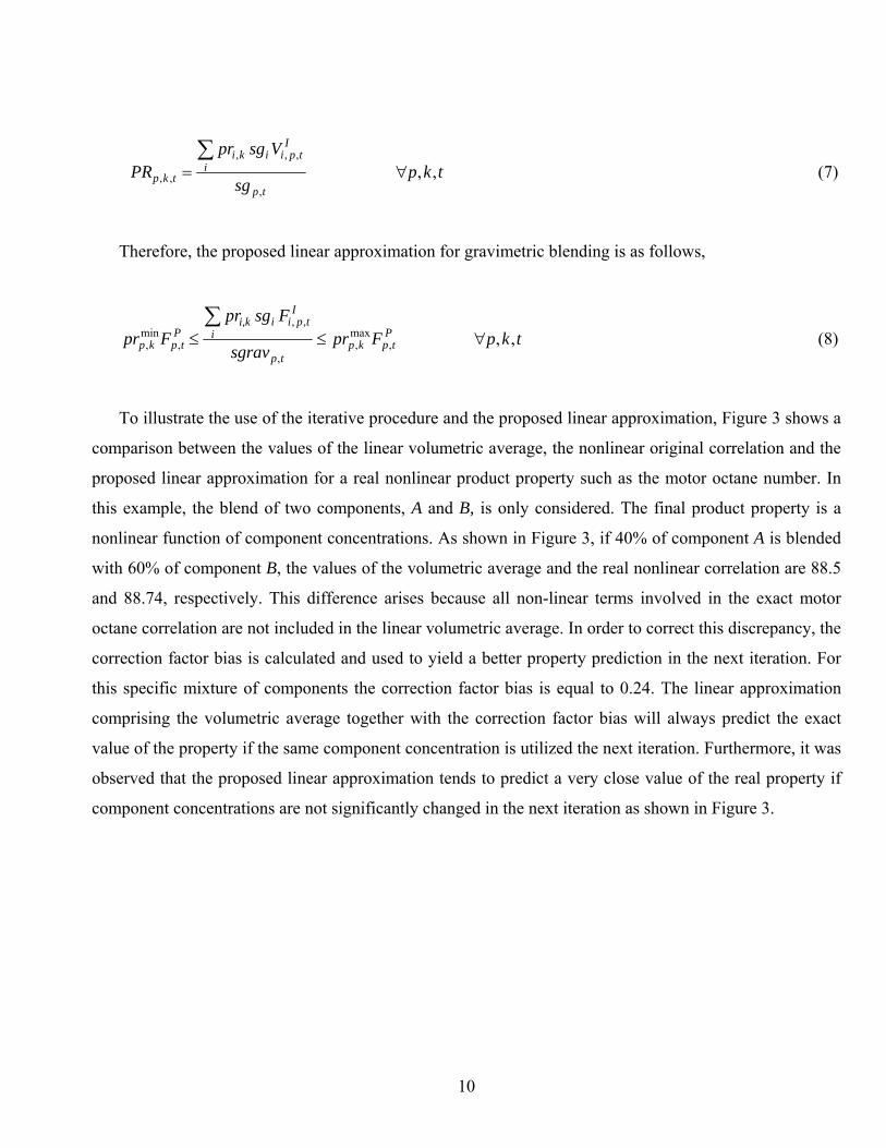
To illustrate the use of the iterative procedure and the proposed linear approximation, Figure 3 shows a

comparison between the values of the linear volumetric average, the nonlinear original correlation and the

proposed linear approximation for a real nonlinear product property such as the motor octane number. In

this example, the blend of two components, A and B, is only considered. The final product property is a

nonlinear function of component concentrations. As shown in Figure 3, if 40% of component A is blended

with 60% of component B, the values of the volumetric average and the real nonlinear correlation are 88.5

and 88.74, respectively. This difference arises because all non-linear terms involved in the exact motor

octane correlation are not included in the linear volumetric average. In order to correct this discrepancy, the

correction factor bias is calculated and used to yield a better property prediction in the next iteration. For

this specific mixture of components the correction factor bias is equal to 0.24. The linear approximation

comprising the volumetric average together with the correction factor bias will always predict the exact

value of the property if the same component concentration is utilized the next iteration. Furthermore, it was

observed that the proposed linear approximation tends to predict a very close value of the real property if

component concentrations are not significantly changed in the next iteration as shown in Figure 3.

11

86

87

88

89

90

91

92

0 0.2 0.4 0.6 0.8 1

Component 'A' volume fraction

prop

erty

Non-linear correlation linear volum. average linear volum. average + bias

Figure 3. A non-linear property and the proposed linear approximation

The proposed iterative procedure to solve simultaneously the blending and scheduling problem using

only linear equations is shown in Figure 4. The first step is to find an initial recipe for all products. If

preferred product recipes are known they can be proposed as initial product recipes. Preferred recipes are

the best alternative for blending because they satisfy all product specifications with minimum cost.

However, the use of them strongly depends on the scheduling decisions, component inventories and

product demands and for this reason, they should not be treated as fixed mixtures in a blending tool. On the

other hand, if preferred recipes are not defined, one possibility for generating initial recipes is to solve the

LP model including only linear product properties. Once initial recipes are generated, they provide the

component volume fractions used in each blend, which can then be employed as fixed parameters in more

realistic non-linear correlations. The value predicted by the non-linear correlation and the linear volumetric

average are both used to calculate the correction factor ‘bias’ (see Figure 3). Given that we are dealing with

a multiperiod optimization problem, the correction factor will be calculated for all non-linear properties,

products and time intervals as the difference between the value predicted by the original non-linear

equation and the linear volumetric average. The specific gravity of each product and time slot is also

computed. After that, the LP model is solved that includes linear approximation with the parameter biasp,k,t,

PPrrooppeerrttyy vvaalluuee CCoommpp AA:: 9922..11 CCoommpp.. BB:: 8866..11

Correction factor ‘bias’ = 0.24

BLEND 40% COMPONENT ‘A’ 60% COMPONENT ‘B’

12

for volumetric properties and the parameter sgravp,k,t, for gravimetric properties. The parameter bias will be

equal to zero for all linear properties that can be computed volumetrically. For nonlinear properties this

parameter will converge to a nonzero value that reflects the difference with the linear approximation.

Subsequently, the solution of this problem is updated and the product recipes for those products meeting all

specifications in a specific time interval are fixed. If different recipes are used for the same product in

different time intervals, only those that are feasible will be fixed. This process is repeated until all product

recipes meet the product specifications, i.e. all product recipes are fixed. The main objective of this

iterative procedure is to progressively find feasible recipes for all products while optimizing all temporal

and resource constraints in the scheduling problem. The proposed method can be conceptually interpreted

as a successive LP method for the blending problem or a successive MILP model for the simultaneous

blending and scheduling problem. Although we have been unable to theoretically prove that the proposed

method converges to the optimal solution, it will be shown later in the paper that only few iterations are

needed to get a very good solution for the blending and scheduling problem, which is particularly relevant

for industrial applications. This has also been confirmed with our experience in solving real world

problems.

Generate initial product recipes

Compute non-linear properties (KNL) for all products and time intervalprp,k,t = gk(vi,p,t ) , where gk(vi,p,t ) is a non-linear correlation for predicting

product property k and vi,p,t is the component volume fraction

Compute correction factor 'bias' and specific gravity 'sgrav'biasp,k,t = g(vi,p,t ) - f(vi,p,t ) where f(vi,p,t ) is the linear volumetric average

sgravp,t =sgp,t where sgp,t is the specific gravity of product p in time interval t

Solve LP Model (blending) orMILP Model (blending and scheduling)

(include all product properties, biasp,k,t and sgravp,t)

Compute non-linear properties (KNL) for all products and time intervalsprp,k,t = g(vi,p,t )

Fix product recipes for products on-spec

All productson-spec

YESIntegrated solution for the blending

and scheduling problem

component volumefractions in blends

component volumefractions in blends

NO

Figure 4. Proposed iterative approach for simultaneous blending and scheduling

13

5. INTEGRATED BLENDING AND SCHEDULING MODEL A central aspect of any scheduling model is related to timing decisions. Mathematical formulations can

be based on either a discrete or continuous time domain representation. The discrete time representation

only allows processing tasks to take place at certain time points, which correspond to the boundaries of a

set of predefined time slots. The main advantage of using a discrete time grid is that mass balance and

inventory constraints are easier to handle but at the same time the solution loses flexibility, unless smaller

time intervals are used, which may significantly decrease the computational performance of the method. In

contrast, continuous time representations are capable of generating more flexible solutions in terms of

timing decisions, although with higher CPU time requirements. Also, inventory and mass balance

constraints are generally more difficult to model since they have to be checked at any time during the

scheduling horizon in order to ensure that a feasible solution will be generated. Since the best choice of the

time representation strongly depends on the problem characteristics and the desired solution quality, we

developed a mathematical formulation for each type of representation assuming a common time grid for all

resources working in parallel. Before presenting the proposed mathematical models the nomenclature is as

follows,

Nomenclature

Indices

d due dates of product demands

i intermediates or components

p final products or gasoline grades

k properties or qualities

t time slots

Sets

D set of product due dates

I set of intermediates to be blended

P set of demanded final products

K set of properties for intermediates and products

KNL set of properties that are predicted with non-linear correlations

T set of time slots

Td set of time slots postulated for the sub-interval ending at due date d (continuous time)

14

Parameters

h time horizon

nBt maximum number of blenders that can be working in parallel in time slot t

st predefined starting time of time slot t (discrete time representation)

et predefined ending time of time slot t (discrete time representation)

ci cost of component i

spi penalty cost for inventory of component i

spp penalty cost for inventory of product p

pltyR+ip penalty cost for excess of component i in product p

pltyR-ip penalty cost for shortage of component i in product p

pltyS+kp penalty cost for a deviation from the minimum specification for property k in product p

pltyS-kp penalty cost for a deviation from the maximum specification for property k in product p

pltySHi penalty cost for purchasing component i from third-party

d demand due date

ddpd demand of product p to be satisfied at due date d

lminp minimum time slot duration when it is allocated to product p

pp price of product p

invi initial inventory of component i

invp initial inventory of product p

Vmini minimum storage capacity of component i

Vmaxi maximum storage capacity of component i

Vminp minimum storage capacity of product p

Vmaxp maximum storage capacity of product p

rcpminip minimum concentration of component i in product p

rcpmaxip maximum concentration of component i in product p

rateminp minimum flow rate of product p

ratemaxp maximum flow rate of product p

rcpip preferred concentration of component i in product p according to product recipe

prik value of property k for component i

prminpk minimum value of property k for product p

prmaxpk maximum value of property k for product p

15

fi constant flowrate of component i

biasp,k,t correction factor of the value of property k of product p in time slot t

sgravp,t specific gravity of product p in time slot t

Variables

FIi,p,t amount of component i being transferred to product p during time slot t

FPp,t amount of product p being blended during time slot t

VIi,t amount of component i stored at the end of time slot t

VPp,t amount of product p stored at the end of time slot t

vIi,p,t volume fraction of component i in product p at time t

PRp,k,t exact value of the property k for product p in time t

St starting time of time slot t (continuous time representation)

Et ending time of time slot t (continuous time representation)

Ap,t binary variable denoting that product p is blended in time slot t

DR-i,p,t shortage of component i that is used for product p in time slot t according to the preferred

product recipe

DR+i,p,t excess of component i that is used for product p in time slot t according to the preferred product

recipe

DS-k,p,t deviation from the minimum specification of property k for product p in time slot t

DS+k,p,t deviation from the maximum specification of property k for product p in time slot t

Si,t amount of component i to be purchased in time slot t

6. DISCRETE TIME REPRESENTATION

In this section we present an MILP model that assumes that the entire scheduling horizon is divided

into a finite number of consecutive time slots that are common for all units and can be allocated to different

products, i.e. blending tasks. The proposed model has the following features:

1. A discrete time domain representation is used where the scheduling horizon is divided into a set of

consecutive time slots.

2. Equivalent blenders working in parallel are available for different product grades.

16

3. A particular product demand can be satisfied by one or more time slots whenever they are allocated to

this product and finished before the product due date.

4. Variable product recipes are considered and product properties are predicted by linear approximations.

5. Constant flow rate of components is assumed during the entire scheduling horizon.

6. Constant flow rate of products is assumed during the allocated time slot.

Model constraints and variables are introduced below.

Allocation constraint

Constraint (9) defines through the binary variables Ap,t the final products p to be processed in time slot

t. Given that a set of equivalent blenders are available to produce different gasoline grades simultaneously,

nBt specifies the maximum number of units that can be working in parallel during time slot t.

t n A Bt

ptp ∀≤∑ , (9)

Product composition constraint

Every final product or gasoline grade p is a blend of different components i, as expressed by constraint

(10)

tp F F Ptp

i

Itpi , ,,, ∀=∑ (10)

Note that a significant reduction in the number of continuous variables can be obtained if equation (10)

is deleted from the model and FPp,t is replaced by ∑iFI

i,p,t. However, in order to make the model easier to

understand, FPp,t has been included in all model equations.

Minimum/maximum component concentration

In order to satisfy product qualities and/or market conditions, upper and lower bounds can be forced on

the component concentration for specific gasoline grades. Then, constraint (11) ensures that product

composition will always satisfy the predefined component specifications. Parameters rcpi,pmin and rcpi,p

max

define the minimum/maximum concentration of component i for product p, respectively,

17

tpiFrcpFFrcp Ptppi

Itpi

Ptppi ,, ,

max,,,,

min, ∀≤≤ (11)

It should be noted that a fixed recipe for a particular product p can also be taken into consideration by

fixing the values of rcpipmin and rcpip

max to the predefined concentration of component i for product p.

However, the use of fixed recipes should be avoided unless they are the only possibility to produce a

particular product. As a better option, preferred recipes can be proposed as an initial solution of the

proposed iterative procedure. In this way, the generation of infeasible solutions will be avoided.

Minimum/maximum volumetric flowrates for products

Constraint (12) specifies that minimum and maximum volumetric flow rates must be satisfied when

product p is blended during time slot t. Due to the fact that a constant product flow rate is assumed in this

work, the volumetric flow rate can be computed by multiplying the upper and lower flowrates by the time

slot duration whenever product p is allocated to a particular time slot t (Ap,t =1). Moreover, since a discrete

time representation is used, the time slot duration is a known parameter computed through the predefined

starting st and ending times et of each time slot t. It should be noted that if product p is not processed during

time slot t, (Ap,t =0), the volumetric flow rate will be also equal to zero.

tpAserateFAserate tpttpP

tptpttp , )()( ,max

,,min ∀−≤≤− (12)

Material balance equation for components

Given that a discrete time representation allows the blending tasks to start and finish at the boundaries

of the time slot allocated, inventory limits have only to be checked at the end of each time slot. Then, as

expressed by constraint (13), the amount of component i being stored in tank at the end of time slot t is

equal to the initial inventory of component i plus the component produced up to the end of time slot t

minus the component transferred to blenders up to the end of time slot t,

tiFefiniVttp

Itpitii

Iti ,

',',,, ∀−+= ∑

≤ (13)

18

where inii is the initial inventory of component i at time t=0, the parameter fi specifies the constant

production rate of component i and et defines the ending time of time slot t. Given that a discrete time

representation is used, both parameters are known in advance.

Component storage capacity

Constraint (14) imposes lower/upper bounds Vimin and Vi

max on the total amount of component i being

stored in a storage tank during the scheduling horizon. Given that constant component flowrates are

assumed, a perfect coordination between the production of components and final products is required to

satisfy the storage constraints through the entire scheduling horizon.

tiVVV iItii , max,

min ∀≤≤ (14)

Material balance equation for products

Constraint (15) computes the amount of product p being stored in tank at the end of time slot t taking

into account the initial inventory, production and demands of product p

tpddFiniVtd

pdtt

ptpp

Ptp ,

'',, ∀−+= ∑∑

≤≤ (15)

Product storage capacity

A minimum safety stock and a finite storage capacity is assumed for final products

tpVVV pP

tpp , max,

min ∀≤≤ (16)

Minimum/maximum product qualities

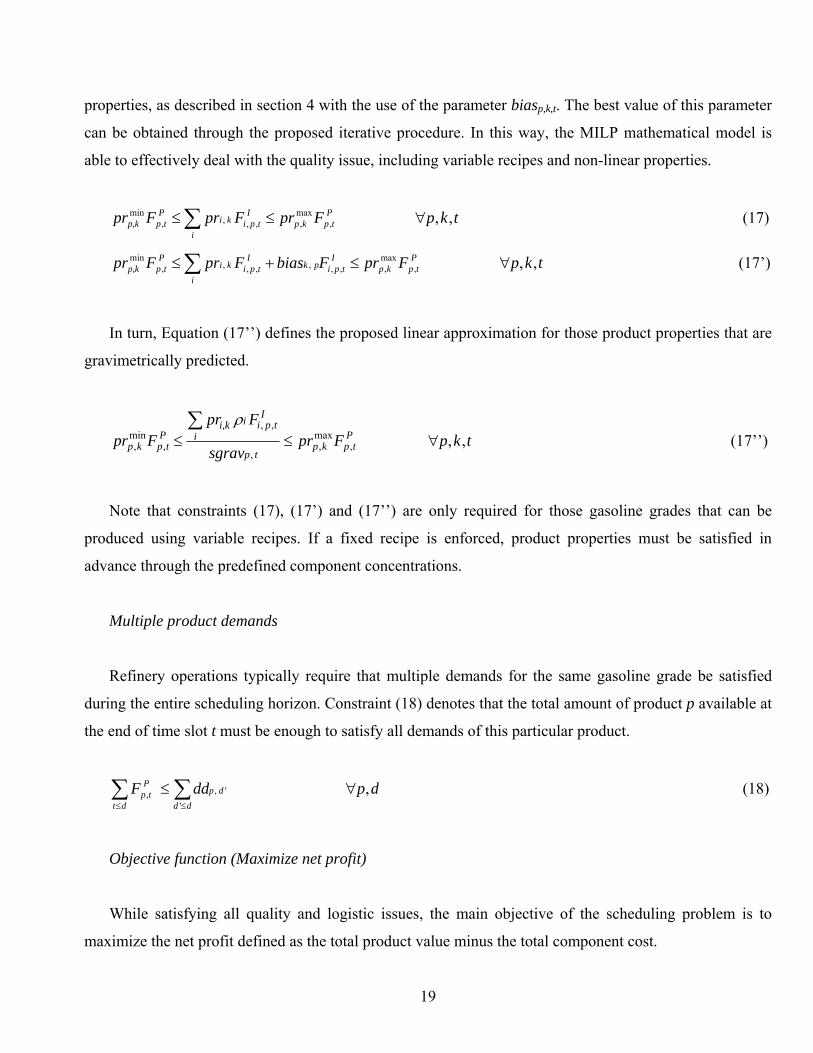
Assuming that properties are volumetrically computed, constraint (17) guarantees that the value of

property k for product p in time slot t will always satisfy minimum and maximum product specifications.

To maintain the model’s linearity, property k is not directly computed and bounds are only imposed on

each property. Otherwise, non-convex bilinear equations would be generated in the model, which would

then become non-linear. Although this linearization is only valid for properties volumetrically computed,

the original equation (17) can be slightly modified as equation (17’) to account for real-world product

19

properties, as described in section 4 with the use of the parameter biasp,k,t. The best value of this parameter

can be obtained through the proposed iterative procedure. In this way, the MILP mathematical model is

able to effectively deal with the quality issue, including variable recipes and non-linear properties.

tkpFprFprFpr Ptpkp

Itpi

i

kiP

tpp,k ,, ,max,,,,,

min ∀≤≤∑ (17)

tkpFprFbiasFprFpr Ptpkp

Itpipk

Itpi

i

kiP

tpp,k ,, ,max,,,,,,,,

min ∀≤+≤∑ (17’)

In turn, Equation (17’’) defines the proposed linear approximation for those product properties that are

gravimetrically predicted.

tkpFprsgrav

FprFpr P

tpkptp

Itpi

iii,k

Ptpkp ,, ,

max,

,

,,

,min, ∀≤≤

∑ ρ (17’’)

Note that constraints (17), (17’) and (17’’) are only required for those gasoline grades that can be

produced using variable recipes. If a fixed recipe is enforced, product properties must be satisfied in

advance through the predefined component concentrations.

Multiple product demands

Refinery operations typically require that multiple demands for the same gasoline grade be satisfied

during the entire scheduling horizon. Constraint (18) denotes that the total amount of product p available at

the end of time slot t must be enough to satisfy all demands of this particular product.

dpdd F dd

dpdt

Ptp , '

',, ∀≤ ∑∑

≤≤

(18)

Objective function (Maximize net profit)

While satisfying all quality and logistic issues, the main objective of the scheduling problem is to

maximize the net profit defined as the total product value minus the total component cost.

20

∑∑ ∑ ⎟⎠

⎞⎜⎝

⎛−

t p

Itpi

i

iP

tpp FcFpMax ,,, (19)

The formulation can also accommodate alternative objective functions. An example is equation (20),

where penalties related to component and product inventories has been included in order to also reduce

storage costs.

∑∑∑∑∑∑ ∑ −−⎟⎠

⎞⎜⎝

⎛−

i t

Itii

p t

Ptpp

t p

Itpi

i

iP

tpp VspVspFcFpMax ,,,,, (20)

7. CONTINUOUS TIME REPRESENTATION

The model introduced the previous section is based on a discrete time domain representation. To

generate more flexible schedules capable of maximizing the plant performance without significantly

increasing the model size, a continuous time formulation is presented in this section. However, special

attention must be paid to the limited storage capacity since continuous time representation tends to make

the modeling of inventory constraints more difficult. The main idea here is first to partition the entire time

horizon into a predefined number of sub-intervals. The size of each sub-interval will depend on the product

due dates. For instance, the first sub-interval will start at the beginning of the scheduling horizon and finish

at the first product due date. The second one will be extended from the first up to the second product due

date. A similar idea is applied to the next sub-intervals. Then, the number of sub-intervals will be equal to

the number of product due dates. In this way, the starting and ending time of each sub-interval is known in

advance.

Once the sub-intervals are defined, a set of time slots with unknown duration are postulated for each

one. The number of time slots for each sub-interval will depend on the sub-interval length as well as the

grade of flexibility desired for the solution. Starting and ending time of time slots will be new continuous

variables, allowing the production events to happen at any time during the scheduling horizon. Figure 5

shows a diagram illustrating the main features of the proposed continuous time domain representation. In

this case, four product demands with different due dates are to be satisfied, which means that 4 sub-

intervals are predefined. Then, nine time slots can be postulated for the entire scheduling horizon, where

21

two time-slots are defined for each one of the first three sub-intervals whereas three are postulated to the

last one.

Figure 5. Proposed continuous time representation

The proposed model has the following features:

1. A continuous time domain representation is used where the scheduling horizon is divided into sub-

intervals and a set of time slots with unknown duration and position are postulated for each one.

2. Equivalent blenders working in parallel are available for different product grades

3. A particular product demand can be satisfied by one or more time slots whenever they are allocated to

this product and finished before product due date.

4. Final product properties are based on a volumetric average and a correction factor computed through

the proposed iterative process.

5. A constant flow rate of components is assumed during the entire scheduling horizon

6. A constant flow rate of product is assumed during the allocated time slot.

When the mathematical model is based on a continuous time domain representation, starting and

ending times for the time slots are new continuous decision variables. For that reason, part of the original

constraints used for the discrete time representation must be updated in order to maintain the linearity of

the model as well as to account new problem features. In this section we describe the set of constraints that

must be modified as well as the new ones to be added. Constraints that are not required to change must be

included into the model in the same way they were presented in the previous section, such as equations (9),

(10), (11), (14), (15), (16), (17), (17’), (17’’), (18), (19).

Product Due Dates D1 D2 D3 D4

time

T1 T2 T3 T4 T5 T6 T7 T8 T9

SLOTS

22

Minimum/maximum volumetric flowrates for products

Constraints (12’) and (12’’) replace original constraint (12) when a continuous time representation is

used. When product p is not allocated to time slot t, the binary variable Ap,t is equal to zero and constraint

(12’’) enforces the variable FPp,t to be equal to zero as well. On the other hand, Ap,t will be equal to one

whenever product p is processed during time slot t. In this case, constraint (12’’) becomes redundant and

constraint (12’) imposes minimum and maximum volumetric flow rates depending on the time slot

duration.

tpSErateFAhrateSErate ttpP

tptppttp , )()1()( max,,

minmin ∀−≤≤−−− (12’)

tpAhrateF tppP

tp , ,max

, ∀≤ (12’’)

Material balance equation for components

To ensure that only feasible solutions are generated, the amount of component stored in tank has to be

checked not only at the end but also at the beginning of each time slot. To make this possible, a new

variable V’Ii,t is included into the model and the original equation (13) is replaced by constraints (13’) and

(13’’). The same idea for computing the inventory of components is applied to these new constraints.

tiFEfiniVttp

Itpitii

Iti ,

',',,, ∀−+= ∑

≤ (13’)

tiFSfiniVttp

Itpitii

Iti , '

',',,, ∀−+= ∑

< (13’’)

Note that despite the fact that Et and St are model variables, both constraints remain linear because a

constant production rate fi is assumed for the components.

Component storage capacity

An additional constraint (14’) is required to impose lower/upper bounds Vimin and Vi

max on the total

amount of component i being stored in tank at the beginning of time slot t.

tiVVV iI

tii , ' max,

min ∀≤≤ (14’)

23

Material balance equation for products

Constraint (15’) computes the inventory of product p at the moment of satisfying the production

demand dp. In this way, a minimum safety stock is guaranteed at any time during the scheduling horizon,

even after a product delivery is carried out.

pdd

pddt

ptpp

Ptp dpddFiniV , '

'',, ∀−+= ∑∑

≤< (15’)

Constraint (16’) explicitly defines the lower bound on the new inventory variable.

tpVV Ptpp , ' ,

min ∀≤ (16’)

Set of time slot timing constraints

Instead of defining starting and ending times of time slots as fixed parameters, a continuous time

representation models these decisions as additional continuous variables to be optimized. In order to allow

more flexible solutions and avoid overlapping time slots, a correct order and sequence between postulated

time slots must be established through the next set of constraints.

Time slot duration

Constraint (21) defines a minimum time slot duration when product p is allocated to time slot t. It is

generally used to model an existing operating condition, but at the same time permits eliminating schedules

using very short time slots, which are usually inefficient in practice.

tpAlSE tpptt , ,min ∀≥− (21)

To ensure that duration of a slot is zero if it is not used, equation (22) is included into the model.

tAhSEp

tptt ∀≤− ∑ , (22)

Time slot sequencing

Constraint (23) establishes a sequence between consecutives time slots t and t+1.

24

tSE tt ∀≤ + )1( (23)

Sub-interval bounds

The set Td comprises all time slots that are postulated for a sub-interval related to a particular due date

d. This sub-interval begins at the previous due date d-1 and finishes at due date d. Constraint (24) defines

that time slots pre-allocated to this sub-interval must start after due date d-1 whereas constraints (25)

imposes that them must end before due date d. The main goal of this assumption is that neither additional

variables nor new constraints are required to establish which time slots can satisfy a specific product

demand. As a result, more flexible schedules can be obtained without increasing the complexity of

inventory constraints.

dt TtdS ∈∀−≥ 1 (24)

dt TtdE ∈∀≤ (25)

Time slot allocation

Constraint (26) imposes an order for using the set of predefined time slots. In other words, a time slot

t+1 can be only allocated to a product p whenever the previous time slot within the same sub-interval has

been used.

dp

tpBt

ptp TttdAnA ∈+∀≤ ∑∑ + )1,(, ,)1(, (26)

8. TREATMENT OF INFEASIBLE SOLUTIONS

The short-term blending and scheduling of oil refinery operations is a very complex and highly-

constrained problem, where even feasible solutions are difficult to find in most of the cases. For that

reason, in this section we present an additional set of variables and equations that define penalties that can

be added to the objective function of the proposed model. These penalties relax some hard problem

specifications that can generate infeasible solutions when real world problems are addressed.

25

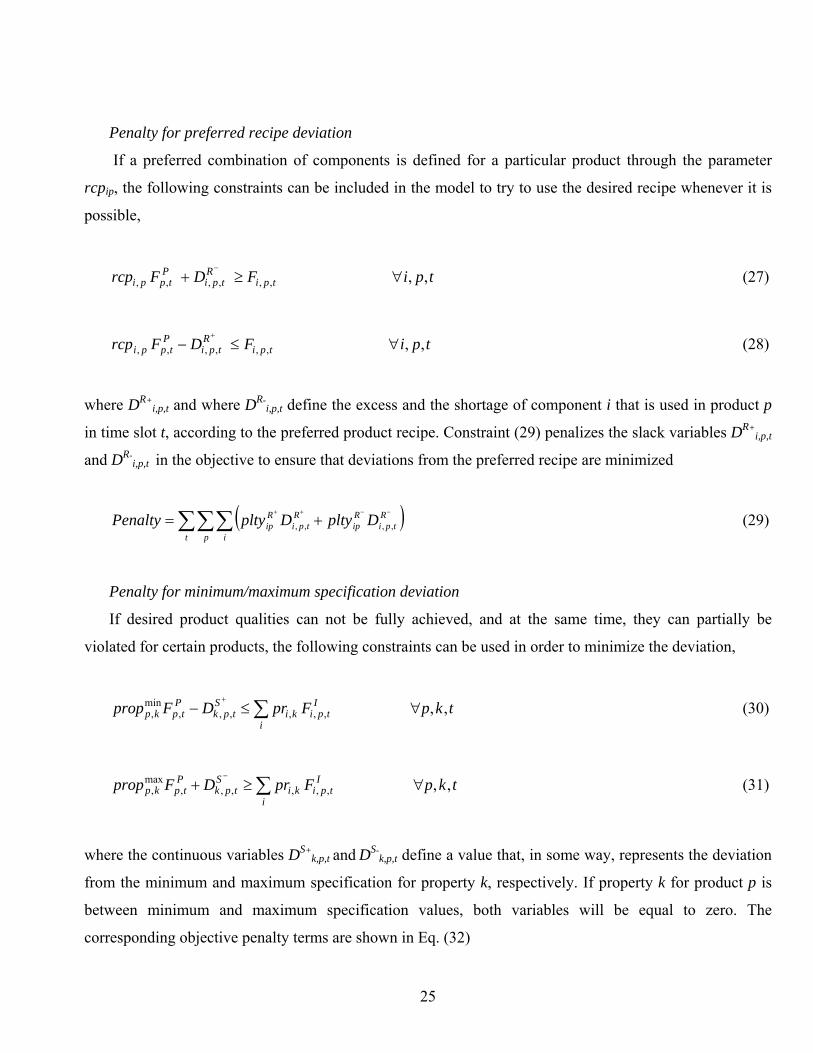
Penalty for preferred recipe deviation

If a preferred combination of components is defined for a particular product through the parameter

rcpip, the following constraints can be included in the model to try to use the desired recipe whenever it is

possible,

tpiF D Frcp tpiR

tpiP

tppi ,, ,,,,, , ∀≥+−

(27)

tpiF DFrcp tpiR

tpiP

tppi ,, ,,,,, , ∀≤−+

(28)

where DR+i,p,t and where DR-

i,p,t define the excess and the shortage of component i that is used in product p

in time slot t, according to the preferred product recipe. Constraint (29) penalizes the slack variables DR+i,p,t

and DR-i,p,t in the objective to ensure that deviations from the preferred recipe are minimized

( )∑∑∑−−++

+=t p i

Rtpi

Rip

Rtpi

Rip DpltyDpltyPenalty ,,,, (29)

Penalty for minimum/maximum specification deviation

If desired product qualities can not be fully achieved, and at the same time, they can partially be

violated for certain products, the following constraints can be used in order to minimize the deviation,

tkpFprDFprop Itpi

iki

Stpk

Ptpkp ,, ,,,,,,

min, ∀≤− ∑

+ (30)

tkpFprDFprop Itpi

iki

Stpk

Ptpkp ,, ,,,,,,

max, ∀≥+ ∑

− (31)

where the continuous variables DS+k,p,t and DS-

k,p,t define a value that, in some way, represents the deviation

from the minimum and maximum specification for property k, respectively. If property k for product p is

between minimum and maximum specification values, both variables will be equal to zero. The

corresponding objective penalty terms are shown in Eq. (32)

26

( )∑∑∑−−++

+=t p k

Stpk

Spk

Stpk

Spk DpltyDpltyPenalty ,,,,,, (32)

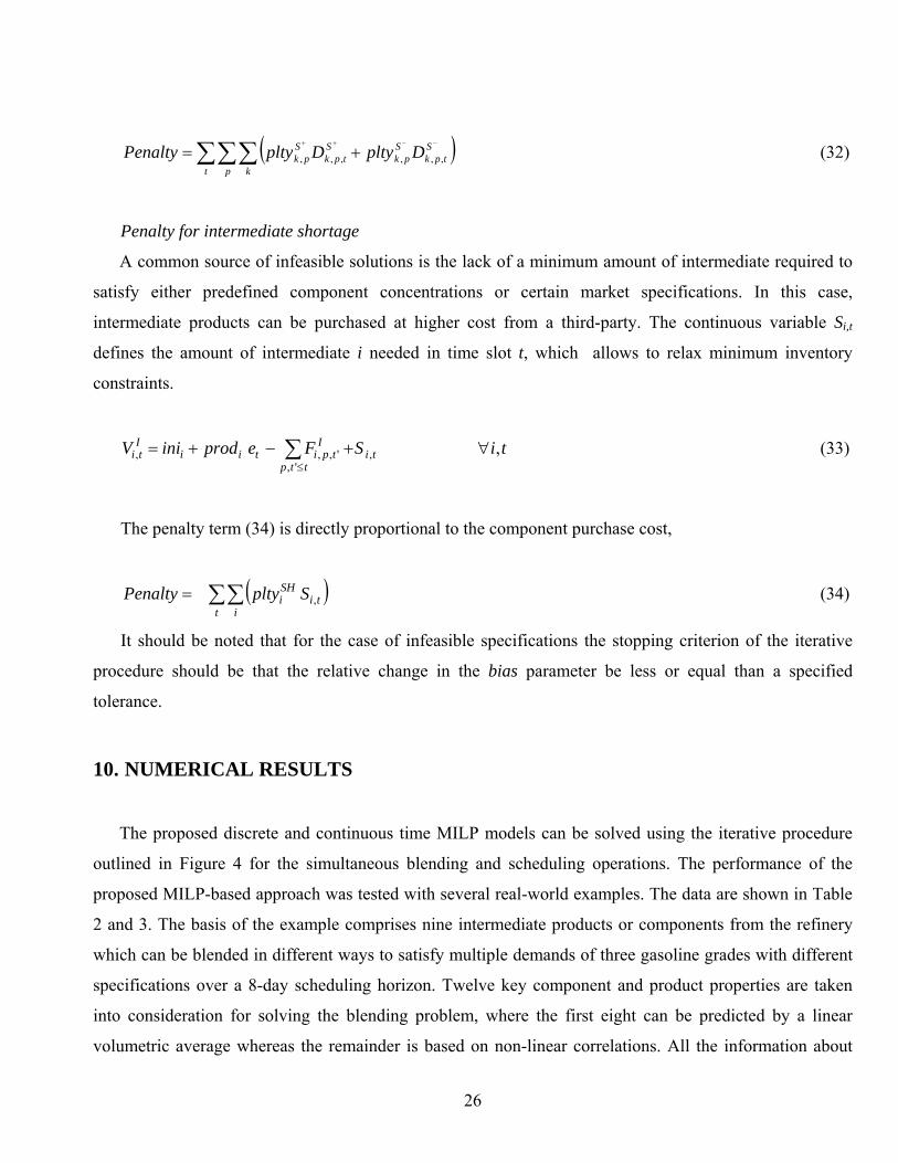
Penalty for intermediate shortage

A common source of infeasible solutions is the lack of a minimum amount of intermediate required to

satisfy either predefined component concentrations or certain market specifications. In this case,

intermediate products can be purchased at higher cost from a third-party. The continuous variable Si,t

defines the amount of intermediate i needed in time slot t, which allows to relax minimum inventory

constraints.

tiSFeprodiniV tittp

Itpitii

Iti , ,

',',,, ∀+−+= ∑

≤ (33)

The penalty term (34) is directly proportional to the component purchase cost,

( )∑∑=t i

tiSHi SpltyPenalty , (34)

It should be noted that for the case of infeasible specifications the stopping criterion of the iterative

procedure should be that the relative change in the bias parameter be less or equal than a specified

tolerance.

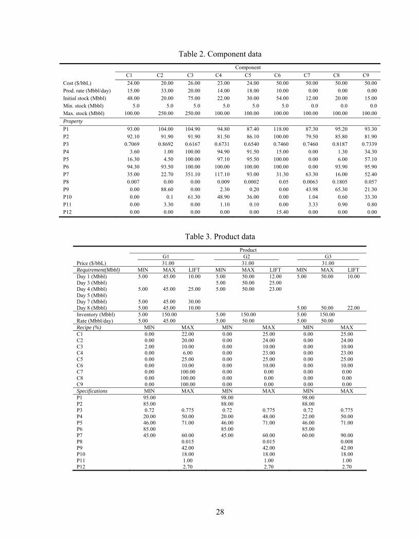
10. NUMERICAL RESULTS The proposed discrete and continuous time MILP models can be solved using the iterative procedure

outlined in Figure 4 for the simultaneous blending and scheduling operations. The performance of the

proposed MILP-based approach was tested with several real-world examples. The data are shown in Table

2 and 3. The basis of the example comprises nine intermediate products or components from the refinery

which can be blended in different ways to satisfy multiple demands of three gasoline grades with different

specifications over a 8-day scheduling horizon. Twelve key component and product properties are taken

into consideration for solving the blending problem, where the first eight can be predicted by a linear

volumetric average whereas the remainder is based on non-linear correlations. All the information about

27

components such as cost, constant production rate, initial, minimum and maximum stocks and properties is

shown in Table 2. Product data including price, requirements, inventory constraints, rate, recipe limits and

specifications are given in Table 3. Dedicated storage tanks with limited capacities for components and

products and three equivalent blend headers working in parallel are available in the refinery. The main goal

is to maximize the total profit, considering component cost, product values and different penalties for

component shortages and out-spec products.

Four different examples were solved with the purpose of analyzing the strong interaction between

blending and scheduling decisions. In order to guarantee that feasible solutions are found, slack variables

for property deviations and intermediate shortages were included in all cases, which were null for all

solutions generated. Example 1 is only focused on the blending problem and its solution is used as initial

product recipes for the other. Examples 2, 3 and 4 are solved using the proposed model with the discrete

and the continuous time domain representation. When the discrete time representation is used, the

scheduling horizon is divided into six consecutive time intervals, where intervals 1, 3, 4 and 6 have 1-day

duration whereas intervals 2 and 5 have 2-day duration. In order to make a direct comparison with the

continuous time formulation, the time discretization is determined based on the product due dates. For the

continuous time representation, one time slot with unknown duration is postulated for each one of the six

subintervals defined by the product due dates.

28

Table 2. Component data Component C1 C2 C3 C4 C5 C6 C7 C8 C9

Cost ($/bbL) 24.00 20.00 26.00 23.00 24.00 50.00 50.00 50.00 50.00 Prod. rate (Mbbl/day) 15.00 33.00 20.00 14.00 18.00 10.00 0.00 0.00 0.00 Initial stock (Mbbl) 48.00 20.00 75.00 22.00 30.00 54.00 12.00 20.00 15.00 Min. stock (Mbbl) 5.0 5.0 5.0 5.0 5.0 5.0 0.0 0.0 0.0 Max. stock (Mbbl) 100.00 250.00 250.00 100.00 100.00 100.00 100.00 100.00 100.00 Property P1 93.00 104.00 104.90 94.80 87.40 118.00 87.30 95.20 93.30 P2 92.10 91.90 91.90 81.50 86.10 100.00 79.50 85.80 81.90 P3 0.7069 0.8692 0.6167 0.6731 0.6540 0.7460 0.7460 0.8187 0.7339 P4 3.60 1.00 100.00 94.90 91.50 15.00 0.00 1.30 34.30 P5 16.30 4.50 100.00 97.10 95.50 100.00 0.00 6.00 57.10 P6 94.30 93.50 100.00 100.00 100.00 100.00 0.00 93.90 95.90 P7 35.00 22.70 351.10 117.10 93.00 31.30 63.30 16.00 52.40 P8 0.007 0.00 0.00 0.009 0.0002 0.05 0.0063 0.1805 0.057 P9 0.00 88.60 0.00 2.30 0.20 0.00 43.98 65.30 21.30 P10 0.00 0.1 61.30 48.90 36.00 0.00 1.04 0.60 33.30 P11 0.00 3.30 0.00 1.10 0.10 0.00 3.33 0.90 0.80 P12 0.00 0.00 0.00 0.00 0.00 15.40 0.00 0.00 0.00

Table 3. Product data Product G1 G2 G3

Price ($/bbL) 31.00 31.00 31.00 Requirement(Mbbl) MIN MAX LIFT MIN MAX LIFT MIN MAX LIFT Day 1 (Mbbl) 5.00 45.00 10.00 5.00 50.00 12.00 5.00 50.00 10.00 Day 3 (Mbbl) 5.00 50.00 25.00 Day 4 (Mbbl) 5.00 45.00 25.00 5.00 50.00 23.00 Day 5 (Mbbl) Day 7 (Mbbl) 5.00 45.00 30.00 Day 8 (Mbbl) 5.00 45.00 10.00 5.00 50.00 22.00 Inventory (Mbbl) 5.00 150.00 5.00 150.00 5.00 150.00 Rate (Mbbl/day) 5.00 45.00 5.00 50.00 5.00 50.00 Recipe (%) MIN MAX MIN MAX MIN MAX C1 0.00 22.00 0.00 25.00 0.00 25.00 C2 0.00 20.00 0.00 24.00 0.00 24.00 C3 2.00 10.00 0.00 10.00 0.00 10.00 C4 0.00 6.00 0.00 23.00 0.00 23.00 C5 0.00 25.00 0.00 25.00 0.00 25.00 C6 0.00 10.00 0.00 10.00 0.00 10.00 C7 0.00 100.00 0.00 0.00 0.00 0.00 C8 0.00 100.00 0.00 0.00 0.00 0.00 C9 0.00 100.00 0.00 0.00 0.00 0.00 Specifications MIN MAX MIN MAX MIN MAX P1 95.00 98.00 98.00 P2 85.00 88.00 88.00 P3 0.72 0.775 0.72 0.775 0.72 0.775 P4 20.00 50.00 20.00 48.00 22.00 50.00 P5 46.00 71.00 46.00 71.00 46.00 71.00 P6 85.00 85.00 85.00 P7 45.00 60.00 45.00 60.00 60.00 90.00 P8 0.015 0.015 0.008 P9 42.00 42.00 42.00 P10 18.00 18.00 18.00 P11 1.00 1.00 1.00 P12 2.70 2.70 2.70

29

10.1. Example 1 (Blending problem)

Example 1 deals with a single-period blending problem of three products (G1, G2, G3). The main goal

is to find the best or ‘preferred’ recipe for each product that minimizes blend cost and simultaneously

satisfies all quality specifications. Preferred recipes are proposed as the initial blends for the subsequent

integrated blending and scheduling examples. For this particular problem, temporal, inventory and resource

constraints coming from the scheduling problem are disregarded by assuming that enough resources,

component stocks and time are available as needed to produce 1 Mbbl of each product once. In this way

only a pure blending problem is taking into consideration. Component cost and properties, variable recipe

limits and stringent product specifications are the central features to be considered for solving Example 1,

where it is assumed that all scheduling decisions are made a priori. The proposed LP-based iterative

procedure was used to find preferred recipes for all required products. As reported in Table 14 in Section

11 on computational results, the problem involves 81 constraints and 127 continuous variables and its

solution was found in 0.13 s. In this case, initial product recipes were generated taking into account only

linear product properties. Then the iterative procedure was performed to update the initial recipes with the

purpose of satisfying all product specifications. Preferred recipes for products G2 and G3 were found by

executing just one iteration of the proposed procedure, whereas an additional iteration was needed to

satisfy all specifications for product G1, since the maximum specification for property P8 was violated

both in the initial recipe as in the first iteration (see Table 4). In order to generate feasible recipes,

component concentrations for each product were updated by the LP model in each iteration, which

gradually increased the blend cost. The recipe evolution for product G1 in terms of component

concentration is presented in detail in Figure 5. Blend cost and product properties associated to each recipe

are shown in Table 4. In addition to the exact values for each property predicted by nonlinear correlations,

the approximations predicted by the proposed linear functions are also presented in Table 4. It should be

noted that predictions of nonlinear properties tend to improve when the number of iterations is increased.

Finally, best product recipes and ‘bias’ factors for all products are reported in Table 5.

30

INITIAL RECIPE

C220

C33.598C4

6

C67.246

C7

C816.156 C1

22

C525

ITERATION 1

C122

C220

C32

C44.938

C525

C610

C75.181

C81.114

C99.767

ITERATION 2

C122

C220

C32

C44.847

C525

C610

C75.198

C80.958

C99.997

C1C2C3C4C5C6C7C8C9

Figure 5. Convergence to preferred recipe for product G1 (iterative procedure)

Table 4. Iterative blending problem for product G1 Min.

Spec. Initial recipe Iteration 1 Iteration 2 Max

Spec. Blend cost ($/bbL) 29.30 29.97 29.99 Quality Value Value Approx. Value Approx. P1 95.00 97.891 97.898 97.7737 97.893 97.8928 P2 85.00 88.417 88.470 88.0493 88.438 88.4335 P3 0.72 0.7418 0.7325 0.7324 0.775 P4 20.00 34.455 35.418 35.409 50.00 P5 46.00 46.00 50.80 50.833 71.00 P6 85.00 96.460 91.797 91.780 P7 45.00 60.00 60.00 60.00 60.00 P8 0.0378 0.0152 0.0150 0.0150 0.0150 0.015 P9 28.458 22.974 22.923 42.00 P10 14.256 15.974 16.005 18.00 P11 0.8964 1.00 1.00 1.00 P12 1.1223 1.5684 1.5488 1.5687 1.5684 2.70

31

Table 5. Preferred product recipes Product G1 G2 G3

Blend cost ($/bbL) 29.99 25.28 24.98 Recipe (%) C1 22.00 25.00 25.00 C2 20.00 23.947 24.00 C3 2.00 16.794 1.372 C4 4.847 25.00 16.636 C5 25.00 9.259 25.00 C6 10.00 7.992 C7 5.198 C8 0.958 C9 9.997 Quality P1 97.893 (bias =1.527) 98.4122 (bias = 1.5611) 98.2214 (bias=1.5208) P2 88.438 (bias = -0.659) 88.4594 (bias = -1.0439) 88.3310 (bias=-1.0861) P3 0.7324 0.7305 0.7289 P4 35.409 41.3410 42.3734 P5 50.833 54.5932 54.5475 P6 91.780 97.0184 97.0150 P7 60.00 60.00 64.2465 P8 0.0150 0.0079 0.0072 P9 22.923 21.6536 21.6966 P10 16.005 17.2363 18.00 P11 1.00 1.00 1.00 P12 1.5687 1.4561 1.2597

10.2. Example 2 (Blending and scheduling with limited production)

In Example 2 preferred product recipes found in Example 1 were used as the initial solution for the

proposed iterative MILP-based procedure. Despite using linear approximations, the proposed MILP model

was capable of finding in just one iteration the same solution generated by nonlinear optimization tools.

However, although the discrete and continuous time representations obtained the same profit in terms of

component cost and product value (1,611,210 $), the continuous time representation is able to find a

schedule that operates the blenders at full capacity for 2.67 days less than the discrete time representation,

which can significantly reduce the total operating cost. Product schedules based on a discrete and

continuous time representation are reported in Tables 6 and 7, respectively. Gantt charts and inventory

evolution of components for both discrete and continuous time representations are shown in Figure 6. As

shown in Table 14, the discrete time formulation involves 679 constraints, 9 binary variables, and 757

continuous variables. The continuous time formulation comprises 832 constraints, 9 binary variables, and

841 continuous variables. Both models were solved in 0.26 s.

32

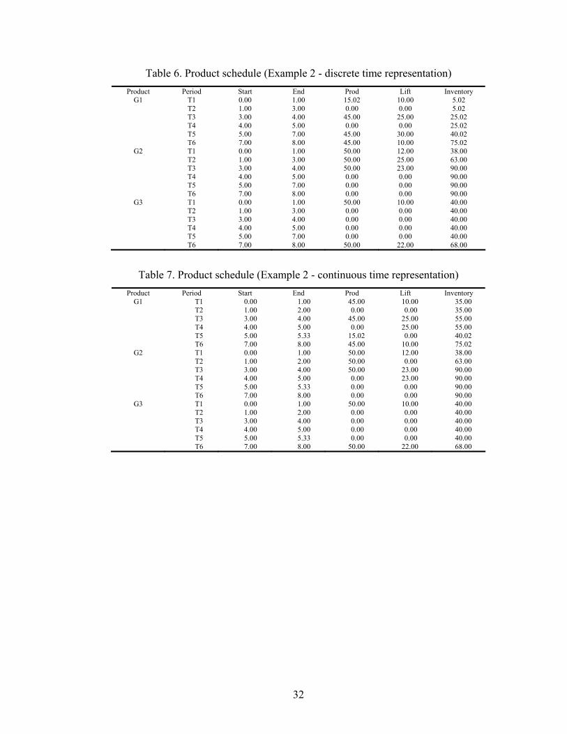
Table 6. Product schedule (Example 2 - discrete time representation) Product Period Start End Prod Lift Inventory

G1 T1 0.00 1.00 15.02 10.00 5.02 T2 1.00 3.00 0.00 0.00 5.02 T3 3.00 4.00 45.00 25.00 25.02 T4 4.00 5.00 0.00 0.00 25.02 T5 5.00 7.00 45.00 30.00 40.02 T6 7.00 8.00 45.00 10.00 75.02

G2 T1 0.00 1.00 50.00 12.00 38.00 T2 1.00 3.00 50.00 25.00 63.00 T3 3.00 4.00 50.00 23.00 90.00 T4 4.00 5.00 0.00 0.00 90.00 T5 5.00 7.00 0.00 0.00 90.00 T6 7.00 8.00 0.00 0.00 90.00

G3 T1 0.00 1.00 50.00 10.00 40.00 T2 1.00 3.00 0.00 0.00 40.00 T3 3.00 4.00 0.00 0.00 40.00 T4 4.00 5.00 0.00 0.00 40.00 T5 5.00 7.00 0.00 0.00 40.00 T6 7.00 8.00 50.00 22.00 68.00

Table 7. Product schedule (Example 2 - continuous time representation) Product Period Start End Prod Lift Inventory

G1 T1 0.00 1.00 45.00 10.00 35.00 T2 1.00 2.00 0.00 0.00 35.00 T3 3.00 4.00 45.00 25.00 55.00 T4 4.00 5.00 0.00 25.00 55.00 T5 5.00 5.33 15.02 0.00 40.02 T6 7.00 8.00 45.00 10.00 75.02

G2 T1 0.00 1.00 50.00 12.00 38.00 T2 1.00 2.00 50.00 0.00 63.00 T3 3.00 4.00 50.00 23.00 90.00 T4 4.00 5.00 0.00 23.00 90.00 T5 5.00 5.33 0.00 0.00 90.00 T6 7.00 8.00 0.00 0.00 90.00

G3 T1 0.00 1.00 50.00 10.00 40.00 T2 1.00 2.00 0.00 0.00 40.00 T3 3.00 4.00 0.00 0.00 40.00 T4 4.00 5.00 0.00 0.00 40.00 T5 5.00 5.33 0.00 0.00 40.00 T6 7.00 8.00 50.00 22.00 68.00

33

a) Discrete time b) Continuous time

0

40

80

120

160

200

240

0 1 2 3 4 5 6 7 8T im e

C1 C2 C3 C4 C5 C6 C7 C8 C9

0

40

80

120

160

200

240

0 1 2 3 4 5 6 7 8T im e

c) Discrete time d) Continuous time

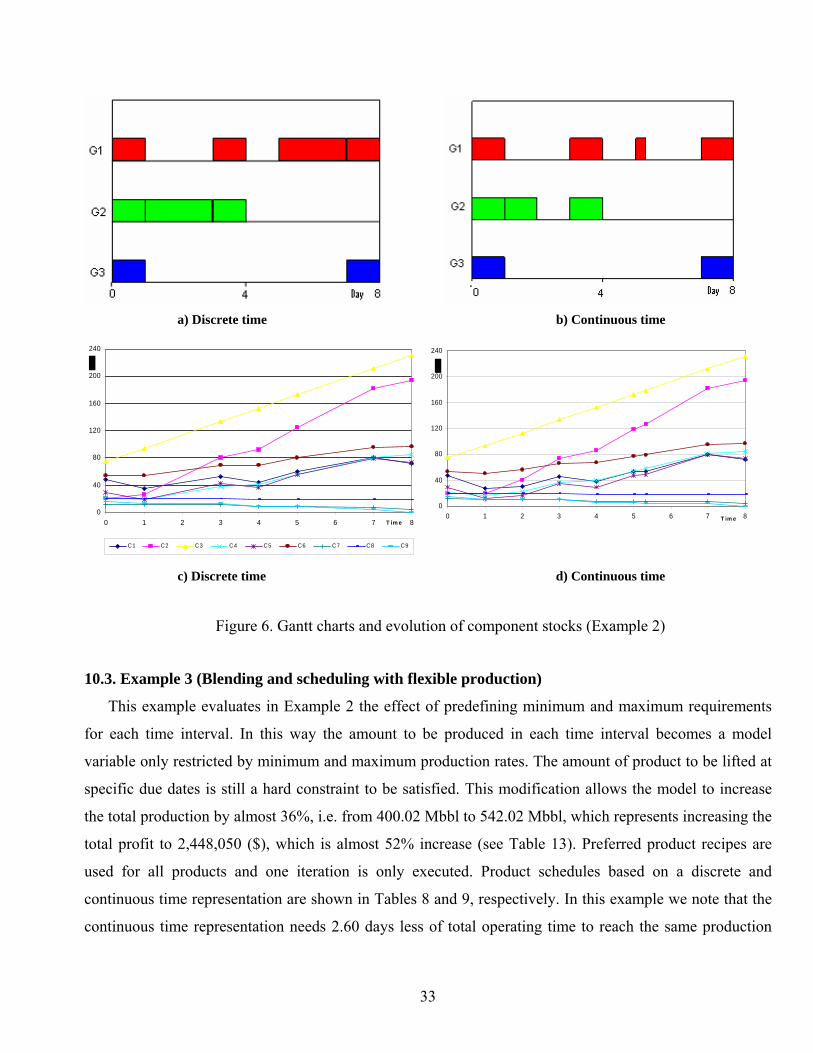
Figure 6. Gantt charts and evolution of component stocks (Example 2)

10.3. Example 3 (Blending and scheduling with flexible production)

This example evaluates in Example 2 the effect of predefining minimum and maximum requirements

for each time interval. In this way the amount to be produced in each time interval becomes a model

variable only restricted by minimum and maximum production rates. The amount of product to be lifted at

specific due dates is still a hard constraint to be satisfied. This modification allows the model to increase

the total production by almost 36%, i.e. from 400.02 Mbbl to 542.02 Mbbl, which represents increasing the

total profit to 2,448,050 ($), which is almost 52% increase (see Table 13). Preferred product recipes are

used for all products and one iteration is only executed. Product schedules based on a discrete and

continuous time representation are shown in Tables 8 and 9, respectively. In this example we note that the

continuous time representation needs 2.60 days less of total operating time to reach the same production

34

level as the discrete time model. Figure 7 shows Gantt-charts and evolution of component stock for

Example 3. The discrete time formulation comprises 679 constraints, 18 binary variables, and 757

continuous variables and its solution was found in 0.23 s. The continuous time formulation comprises 832

constraints, 18 binary variables, and 841 continuous variables and its solution was generated in 0.26 s. (see

Table 14).


G1 T1 0.00 1.00 45.00 10.00 35.00 T2 1.00 3.00 60.02 0.00 95.02 T3 3.00 4.00 0.00 25.00 70.02 T4 4.00 5.00 0.00 0.00 70.02 T5 5.00 7.00 0.00 30.00 40.02 T6 7.00 8.00 45.00 10.00 75.02

G2 T1 0.00 1.00 50.00 12.00 38.00 T2 1.00 3.00 0.00 25.00 13.00 T3 3.00 4.00 50.00 23.00 40.00 T4 4.00 5.00 0.00 0.00 40.00 T5 5.00 7.00 60.00 0.00 100.00 T6 7.00 8.00 50.00 0.00 150.00

G3 T1 0.00 1.00 50.00 10.00 40.00 T2 1.00 3.00 72.00 0.00 112.00 T3 3.00 4.00 0.00 0.00 112.00 T4 4.00 5.00 0.00 0.00 112.00 T5 5.00 7.00 10.00 0.00 122.00 T6 7.00 8.00 50.00 22.00 150.00


G1 T1 0.00 1.00 45.00 10.00 35.00 T2 2.80 3.00 9.00 10.00 44.00 T3 3.00 4.00 45.00 35.00 64.00 T4 4.00 4.80 4.00 35.00 68.00 T5 6.80 7.00 9.00 65.00 47.00 T6 7.00 8.00 38.02 75.00 75.02

G2 T1 0.00 1.00 50.00 12.00 38.00 T2 2.80 3.00 10.00 37.00 23.00 T3 3.00 4.00 50.00 60.00 50.00 T4 4.00 4.80 40.00 60.00 90.00 T5 6.80 7.00 10.00 60.00 100.00 T6 7.00 8.00 50.00 60.00 150.00

G3 T1 0.00 1.00 50.00 10.00 40.00 T2 2.80 3.00 0.00 10.00 40.00 T3 3.00 4.00 50.00 10.00 90.00 T4 4.00 4.80 40.00 10.00 130.00 T5 6.80 7.00 10.00 10.00 140.00 T6 7.00 8.00 32.00 32.00 150.00

35

a) Discrete time b) Continuous time

0

40

80

120

160

200

240

0 1 2 3 4 5 6 7 8T ime 0

40

80

120

160

200

240

0 1 2 3 4 5 6 7 8T ime

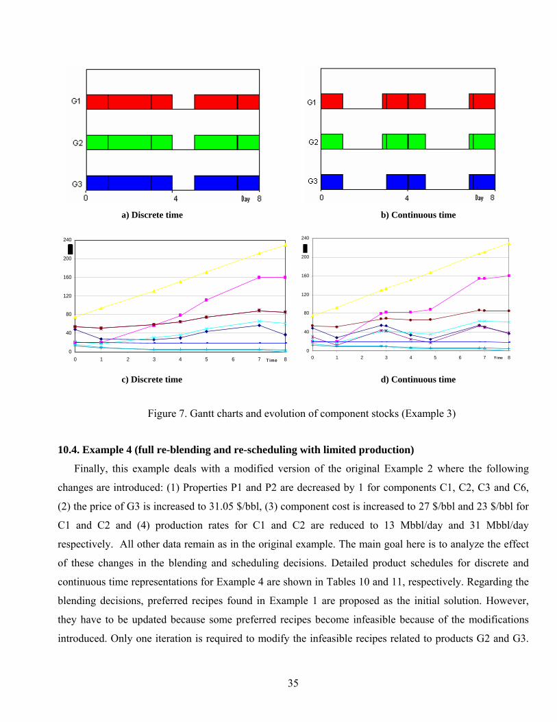
c) Discrete time d) Continuous time

Figure 7. Gantt charts and evolution of component stocks (Example 3)

10.4. Example 4 (full re-blending and re-scheduling with limited production)

Finally, this example deals with a modified version of the original Example 2 where the following

changes are introduced: (1) Properties P1 and P2 are decreased by 1 for components C1, C2, C3 and C6,

(2) the price of G3 is increased to 31.05 $/bbl, (3) component cost is increased to 27 $/bbl and 23 $/bbl for

C1 and C2 and (4) production rates for C1 and C2 are reduced to 13 Mbbl/day and 31 Mbbl/day

respectively. All other data remain as in the original example. The main goal here is to analyze the effect

of these changes in the blending and scheduling decisions. Detailed product schedules for discrete and

continuous time representations for Example 4 are shown in Tables 10 and 11, respectively. Regarding the

blending decisions, preferred recipes found in Example 1 are proposed as the initial solution. However,

they have to be updated because some preferred recipes become infeasible because of the modifications

introduced. Only one iteration is required to modify the infeasible recipes related to products G2 and G3.

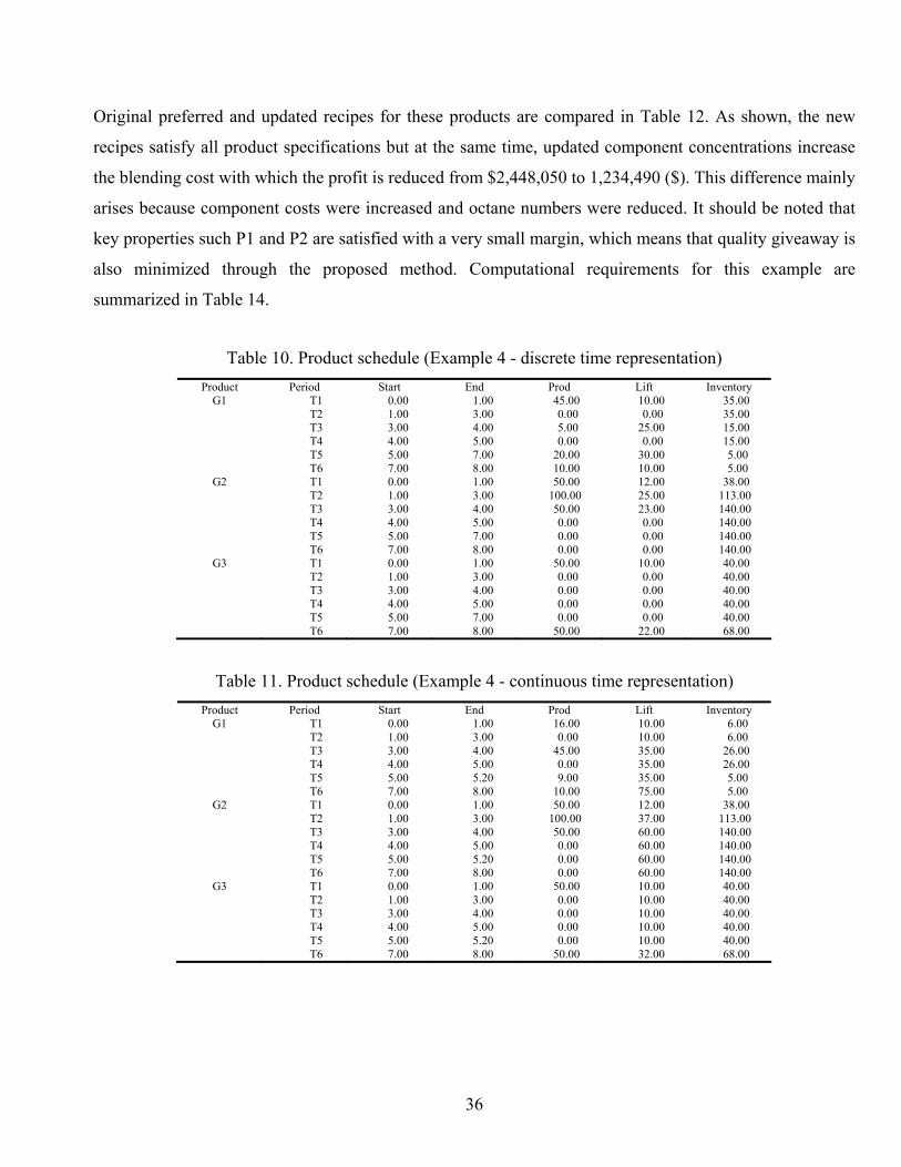
36

Original preferred and updated recipes for these products are compared in Table 12. As shown, the new

recipes satisfy all product specifications but at the same time, updated component concentrations increase

the blending cost with which the profit is reduced from $2,448,050 to 1,234,490 ($). This difference mainly

arises because component costs were increased and octane numbers were reduced. It should be noted that

key properties such P1 and P2 are satisfied with a very small margin, which means that quality giveaway is

also minimized through the proposed method. Computational requirements for this example are

summarized in Table 14.


G1 T1 0.00 1.00 45.00 10.00 35.00 T2 1.00 3.00 0.00 0.00 35.00 T3 3.00 4.00 5.00 25.00 15.00 T4 4.00 5.00 0.00 0.00 15.00 T5 5.00 7.00 20.00 30.00 5.00 T6 7.00 8.00 10.00 10.00 5.00

G2 T1 0.00 1.00 50.00 12.00 38.00 T2 1.00 3.00 100.00 25.00 113.00 T3 3.00 4.00 50.00 23.00 140.00 T4 4.00 5.00 0.00 0.00 140.00 T5 5.00 7.00 0.00 0.00 140.00 T6 7.00 8.00 0.00 0.00 140.00

G3 T1 0.00 1.00 50.00 10.00 40.00 T2 1.00 3.00 0.00 0.00 40.00 T3 3.00 4.00 0.00 0.00 40.00 T4 4.00 5.00 0.00 0.00 40.00 T5 5.00 7.00 0.00 0.00 40.00 T6 7.00 8.00 50.00 22.00 68.00


G1 T1 0.00 1.00 16.00 10.00 6.00 T2 1.00 3.00 0.00 10.00 6.00 T3 3.00 4.00 45.00 35.00 26.00 T4 4.00 5.00 0.00 35.00 26.00 T5 5.00 5.20 9.00 35.00 5.00 T6 7.00 8.00 10.00 75.00 5.00

G2 T1 0.00 1.00 50.00 12.00 38.00 T2 1.00 3.00 100.00 37.00 113.00 T3 3.00 4.00 50.00 60.00 140.00 T4 4.00 5.00 0.00 60.00 140.00 T5 5.00 5.20 0.00 60.00 140.00 T6 7.00 8.00 0.00 60.00 140.00

G3 T1 0.00 1.00 50.00 10.00 40.00 T2 1.00 3.00 0.00 10.00 40.00 T3 3.00 4.00 0.00 10.00 40.00 T4 4.00 5.00 0.00 10.00 40.00 T5 5.00 5.20 0.00 10.00 40.00 T6 7.00 8.00 50.00 32.00 68.00

37

Table 12. Updated product recipes (Example 4) Product G2 G3

Preferred Updated Preferred Updated Blend cost ($/bbL) 25.28 26.92 24.98 26.67 Recipe (%) C1 25.00 25.00 25.00 25.00 C2 23.947 24.00 24.00 24.00 C3 16.794 0.223 1.372 3.195 C4 25.00 16.09 16.636 14.869 C5 9.259 24.831 25.00 24.269 C6 9.856 7.992 8.640 Quality P1 97.8204 98.0235 97.6283 98.052 P2 87.8588 88.0133 87.7294 88.0455 P3 0.7305 0.7309 0.7289 0.7285 P4 41.3408 40.831 42.3734 41.9724 P5 54.5936 54.571 54.5476 54.6305 P6 97.0184 97.015 97.015 97.015 P7 60.00 60.00 64.2473 68.1274 P8 0.0079 0.0081 0.0072 0.0074 P9 21.6533 21.6837 21.6966 21.6546 P10 17.2362 16.968 18.00 18.00 P11 1.00 0.9938 1.00 0.9799 P12 1.4562 1.5491 1.2597 1.3626

11. COMPUTATIONAL RESULTS

Different blending and scheduling problems were solved in the previous section in order to evaluate the

efficiency of the proposed method. Example 1 dealt with a pure blending problem whereas examples 2, 3

and 4 also accounted optimal scheduling decisions. Examples 3 and 4 correspond to modified versions of

the original Example 2 where minimum and maximum requirements were relaxed (Example 3) and certain

changes in component properties and cost and product prices were incorporated (Example 4). Table 13

summarizes the results for examples 2, 3 and 4, while Table 14 provides the computational statistics on the

four examples. As can be seen, the size of the MILP problems is not very large and involves a modest

number of 0-1 variables. For this reason every single problem needs no more than 1 sec at CPU time with

CPLEX 8.1, which highlights the computational efficiency of the proposed models and the iterative MILP

procedure. In addition, a very small number of iterations were required to satisfy all product specifications

in all the examples. The method found more economic solutions to a combined blending and scheduling

problem almost one order of magnitude faster than it took to solve only the blending NLP problem with a

predetermined schedule (see Table 14). The NLP model was solved on a Pentium IV PC using CONOPT

in GAMS 21.2. As a general characteristic, it was observed that discrete time formulations usually have a

better computational performance when compared to continuous models. On the other hand, continuous

38

formulations are able to generate more flexible schedules that significantly reduce the operating time of the

available equipment.

Table 13. Summary of results Example Blend value Comp. stock

production Comp. inventory

build Total Profit

Profit / BBL

2 12,400,610 22,352,000 11,562,600 1,611,210 4.03 3 16,802,610 22,352,000 7,997,440 2,448,050 4.52 4 11,785,000 23,504,000 12,953,490 1,234,490 3.25

Table 14. Model size and computational requirements Example Binary vars, cont. vars, constraints CPU time Iterations

1 - , 127,81 0.13 2 2.(NLP model*) -, 919 ,772 1.25b -

2.discrete 9 , 757, 679 0.26a 1 2.continuous 9 , 841, 832 0.26a 1



a Seconds on Pentium IV PC with CPLEX 8.1 in GAMS 21.2 - *All scheduling decisions are predefined b Seconds on Pentium IV PC with CONOPT in GAMS 21.2

12. CONCLUSIONS

An integrated MILP-based approach has been proposed to optimize the gasoline short-term blending

and scheduling problem. The method is able to deal with non-linear product properties and variable recipes

through an iterative procedure that can be used on a discrete or a continuous time formulation. As shown in

the examples, the proposed model can generate very good solutions in terms of profit with very low CPU

time requirements.

Acknowledgements

The authors would like to thank ABB Corporate Research and CAPD Center at CMU for financial

support of this work.

REFERENCES Betchel Corp. (1993). PIMS (Process Industry Modeling System). User’s manual, version 6.0. Houston. TX.

Booner and Moore. (1979). Management Science. RPMS. (Refinery and Petrochemical Modeling System). A system

description, Houston, TX.

Floudas C.A. and Lin X. C. (2004). Continuous-time versus discrete-time approaches for scheduling of chemical

processes: a review. Computers and Chemical Engineering, 28, 2109.

39

Glismann K., Gruhn G. (2001). Short-term scheduling and recipe optimization of blending processes. Computers and

Chemical Engineering, 25, 627.

Grossmann I.E., Van den Heever S.A. and Harjunkoski I. (2002). Discrete optimization methods and their role in the

integration of planning and scheduling. AIChE Symposium Series No. 326, 98, 150.

Kallrath J. (2003). Planning and scheduling in the process industry. Advanced planning and scheduling solutions in

process industry, Springer-Verlag. ISBN 3-540-00222-7. 11.

Kelly J.D., Mann J.L. (2002). Crude-oil blend scheduling optimization: An application with multi-million dollar

benefits. Honeywell Hi-Spec Solutions. Personal Communication.

Kelly J.F. (2004). Formulating production planning models. Information Technology. 43.

Lee H., Pinto J.M, Grossmann I.E., Park S. (1996). Mixed-integer linear programming model for refinery short-term

scheduling of crude oil unloading with inventory management. Industrial Engineering & Chemistry Research.

35, 1630.

Moro L.F.L, Zanin A.C., Pinto J.M. (1998). A planning model for refinery diesel production. Computers and

Chemical Engineering, 22, S1039.

Pinto J.M. and Grossmann I.E. (1998). Assignment and sequencing models for the scheduling of chemical processes.

Annals of Operation Research, 81, 433.

Quesada I., Grossmann I.E. (1995). Global optimization of bilinear process networks with multicomponents flows.

Computers and Chemical Engineering, 19, 1219.

Reklaitis G.V. (1992). Overview of scheduling and planning of batch process operations. Technical report, NATO

Advanced Study Institute, Antalaya, Turkey.

Rigby B., Lasdon L.S., and Waren A.D. (1995). The evolution of Texaco blending systems – from Omega to

StarBlend. Interfaces, 25, 64.

Shah, N. (1998). Single- and multisite planning and scheduling: Current status and future challenges. AIChE

Symposium Series No 320, 94, 75.

Jia Z., Iearapetritou M. (2003). Mixed-integer linear programming for gasoline blending and distribution scheduling.

Industrial Engineering & Chemistry Research, 42, 825.

A Simultaneous Optimization Approach for Off-line Blending ...

Documents

Transcript of A Simultaneous Optimization Approach for Off-line Blending ...