A simulation study of Unified GPS and Roadside Ranging Technologies...

QUEENSLAND UNIVERSITY OF TECHNOLOGY

Faculty of Science and Technology

A simulation study of Unified GPS and Roadside

Ranging Technologies for Vehicle Positioning A thesis submitted in partial fulfilment of the requirements for

the degree of

Master by Research

Zhaolei Feng

9/16/2011

ii

Abstract

The future vehicle navigation for safety applications requires seamless positioning at

the accuracy of sub-meter or better. However, standalone Global Positioning System

(GPS) or Differential GPS (DGPS) suffer from solution outages while being used in

restricted areas such as high-rise urban areas and tunnels due to the blockages of

satellite signals. Smoothed DGPS can provide sub-meter positioning accuracy, but

not the seamless requirement. A disadvantage of the traditional navigation aids such

as Dead Reckoning and Inertial Measurement Unit onboard vehicles are either not

accurate enough due to error accumulation or too expensive to be acceptable by the

mass market vehicle users. One of the alternative technologies is to use the wireless

infrastructure installed in roadside to locate vehicles in regions where the Global

Navigation Satellite Systems (GNSS) signals are not available (for example: inside

tunnels, urban canyons and large indoor car parks). The examples of roadside

infrastructure which can be potentially used for positioning purposes could include

Wireless Local Area Network (WLAN)/Wireless Personal Area Network (WPAN)

based positioning systems, Ultra-wide band (UWB) based positioning systems,

Dedicated Short Range Communication (DSRC) devices, Locata’s positioning

technology, and accurate road surface height information over selected road

segments such as tunnels. This research reviews and compares the possible wireless

technologies that could possibly be installed along roadside for positioning purposes.

Models and algorithms of integrating different positioning technologies are also

presented. Various simulation schemes are designed to examine the performance

benefits of united GNSS and roadside infrastructure for vehicle positioning. The

results from these experimental studies have shown a number of useful findings. It is

clear that in the open road environment where sufficient satellite signals can be

obtained, the roadside wireless measurements contribute very little to the

improvement of positioning accuracy at the sub-meter level, especially in the dual

constellation cases. In the restricted outdoor environments where only a few GPS

satellites, such as those with 45 elevations, can be received, the roadside distance

measurements can help improve both positioning accuracy and availability to the

iii

sub-meter level. When the vehicle is travelling in tunnels with known heights of

tunnel surfaces and roadside distance measurements, the sub-meter horizontal

positioning accuracy is also achievable. Overall, simulation results have

demonstrated that roadside infrastructure indeed has the potential to provide sub-

meter vehicle position solutions for certain road safety applications if the properly

deployed roadside measurements are obtainable.

iv

Acknowledgement

I have taken efforts in this report. However, it would not have been possible to

complete without the kind support and help of many people. I would like to extend

my sincere thanks to all of them.

Firstly, I am highly indebted to my principal supervisor Professor Yanming Feng and

associate supervisor A/Professor Glen Tian for their guidance and constant

supervision. They brought me into the field of positioning using GPS/GNSS and

wireless communications and provide large amount of resources for me to facilitate

my research. During the process, they also checked regularly and make sure that I

was on the right track. In addition, they spent great amount of time and effort

checking my report with great patience and gave me lots invaluable suggestions.

I would like to express my gratitude to Dr Charles Wang for his support in a variety of

ways especially his helps in GPS positioning area. Also, he gave me lots of feedbacks

and detailed suggestions for my report based on his advanced knowledge in GPS

area. I also need to thank Mr Hang Jin who is expert at survey area. He helped me a

lot in setting up the simulation environment.

Computational resources and services used in this research were provided by the

Research Support Group, Queensland University of Technology (QUT). I gratefully

acknowledge QUT and School of Information Technology for providing such great

support for my study.

My thanks and appreciations also go to my family and my friends for their

unwavering cooperation and encouragement during my study and my life.

v

Statement of Authorship

“The work contained in this report has not been previously submitted to meet

requirements for an award at this or any other higher education institution. To the

best of my knowledge and belief, this research contains no material previously

published or written by another person except where due reference is made.”

Signature ______________________

Zhaolei Feng

Date ______________________

vi

Table of Contents

Acknowledgement ................................................................................................ iv

Statement of Authorship ........................................................................................ v

Table of Contents .................................................................................................. vi

List of Tables ....................................................................................................... viii

List of Figures ........................................................................................................ ix

Abbreviations ....................................................................................................... xi

1 Introduction ................................................................................................... 1

1.1 Background ..................................................................................................... 1

1.2 Research problems and contributions ............................................................. 6

1.3 Structure of the thesis ..................................................................................... 8

2 GNSS-based positioning systems and techniques for vehicle navigation

systems ................................................................................................................ 9

2.1 Overview of GNSS ............................................................................................ 9

2.2 Global Positioning System ............................................................................. 10

2.3 GNSS Pseudo-range and carrier-phase measurements ................................ 11

2.4 DGPS and smoothed DGPS techniques .......................................................... 14

2.5 Absolute and relative vehicle positioning ..................................................... 18

2.6 Outlook for next generation vehicle positioning system for road safety ...... 19

3 Overview of Roadside wireless communications technologies for positioning

purposes .............................................................................................................. 21

3.1 Cellular Networks .......................................................................................... 21

3.2 WLAN/WiFi .................................................................................................... 23

3.3 WPAN/Bluetooth ........................................................................................... 24

3.4 UWB Based Positioning ................................................................................. 25

3.5 Locata Technologies ...................................................................................... 27

3.6 Dedicated Short Range Communications (DSRC) based positioning ............ 30

vii

4 Mathematical models and estimation algorithms of integrated wireless

positioning ........................................................................................................... 36

4.1 Positioning with TOA measurements ............................................................ 36

4.2 Positioning with TDOA measurements .......................................................... 39

5 Simulations ................................................................................................... 43

5.1 Simulation Platform ...................................................................................... 43

5.2 Definition of the GPS/GNSS constellations and roadside infrastructure ....... 45

5.3 Vehicle Track simulation ............................................................................... 47

5.4 Case Studies of GNSS and RSU signal availability ......................................... 49

5.5 Computational scenarios ............................................................................... 52

6 Experimental results ..................................................................................... 53

6.1 DGPS/GNSS solutions with the noise STD of 1, 0.5, and 0.25m .................... 54

6.2 DGPS+RSU solutions with the noise STD of 1, 0.5, and 0.25m ...................... 55

6.3 GPS+RSU+OBU with the measurement STD of 1m, 0.5m and 0.25m ........... 59

6.4 GNSS +RSUs with the noise STD of 1m, 0.5 m and 0.25 m ............................ 64

6.5 GNSS, RSUs and OBU with the measurement noise STD of 1, 0.5 and 0.25m

67

6.6 RSUs + OBU with measurement noise STD of 1, 0.5, 0.25, 0.15, and 0.1m .. 70

7. Conclusions ................................................................................................... 72

References ........................................................................................................... 74

Appendix A .......................................................................................................... 78

Appendix B .......................................................................................................... 80

viii

List of Tables

Table 1.1 The initial requirements for selected features of the ITS safety applications

................................................................................................................................ 3

Table 1.2: Comparisons of autonomous positioning techniques .................................. 5

Table 2.1: Comparison of Global Navigation Satellite Systems ..................................... 9

Table 2.2: Summary of positioning accuracy Standard Deviation (STD) achievable

with various GNSS-based positioning techniques available for vehicle positioning.

.............................................................................................................................. 19

Table 3.1: Comparison of GSM, CDMA, and WCDMA ................................................. 22

Table 3.2: Specification summary of Locata system .................................................... 28

Table 3.3: Comparison of Locata, DSRC, UWB, Bluetooth, and WiFi .......................... 34

Table 5.1: Computation schemes of simulation .......................................................... 52

ix

List of Figures

Figure 2.1: Global Positioning System Satellite Orbits ................................................ 10

Figure 2.2: Differential GPS Schematic diagram (Courtesy of Matt Higgins) .............. 16

Figure 2.3: Network-based DGPS diagram (Courtesy of Matt Higgins) ....................... 17

Figure 2.4: Victoria CORS network (Courtesy of James Millner) ................................. 17

Figure 3.1: Typical deployment of a Cellular Network ................................................ 21

Figure 3.2: Concept of Vehicle to Vehicle and Vehicle to Roadside communications 32

Figure 3.3: Onboard unit components and process diagram ...................................... 33

Figure 4.1: Two-dimensional three roadside base stations deployment for mobile

station positioning using TOA method ................................................................. 37

Figure 4.2: Two-dimensional three base stations deployment for target positioning

using TDOA method .............................................................................................. 40

Figure 4.3: TDOA method with noises and other impairments ................................... 42

Figure 5.1: Location of roadside units in the simulated test areas ............................. 44

Figure 5.2: Illustration of mask angle in open and low-rise building area .................. 46

Figure 5.3. Illustration of Mask Angle due to in high-rise buildings ............................ 46

Figure 5.4: Layout of RSUs in a tunnel ......................................................................... 47

Figure 5.5: Map to set up vehicle track ....................................................................... 48

Figure 5.6: Matlab visualization of the vehicle tracks ................................................. 48

Figure 5.7: Both GPS and RSU signals are fully available ............................................. 49

Figure 5.8: The case when GPS signals are partially unavailable ................................ 50

Figure 5.9: The case when OBU links are unavailable ................................................. 51

Figure 5.10: GPS signals are completely unavailable................................................... 51

Figure 6.1: Illustration of positioning solutions from GPS only, GPS+RSU and

GPS+RSU+OBU ...................................................................................................... 53

Figure 6.2a: Comparison of the STD value for GPS only positioning. .......................... 54

Figure 6.2b: STD values for GNSS only solutions ......................................................... 55

Figure 6.3a: The relationship between GPS available satellites, available RSUs, and

HDOP when mask angle = 15 ................................................................................ 56

x

Figure 6.3b: STD value of GPS and GPS+RSUs positioning accuracy when mask angle =

15 .......................................................................................................................... 56



Figure 6.4b: STD value of GPS and GPS+RSUs positioning accuracy when mask angle =

30 .......................................................................................................................... 57



Figure 6.5b: STD value of GPS and GPS+RSU with the mask angle of 45 degrees and

the number of available satellites is more than or equals to 4............................ 58

Figure 6.5c: STD value of GPS+RSU solutions with the mask angle = 45 and the

number of satellites is 3 or less ............................................................................ 59

Figure 6.6a: The relationship between the available GPS satellites, available RSUs,

and HDOP when mask angle = 15 ......................................................................... 60

Figure 6.6b: STD value of the GPS+RSUs+OBUs solutions when mask angle = 15 ...... 61

Figure 6.7a: Available GPS satellites, available RSUs+OBUs and HDOP when mask

angle = 30.............................................................................................................. 61

Figure 6.7b: STD value of the GPS and the GPS+RSUs+OBUs positioning solutions

when mask angle = 30 .......................................................................................... 62

Figure 6.8a: The relationship between the available GPS satellites, available

RSUs+OBUs (refs), and HDOP when mask angle = 45 .......................................... 62

Figure 6.8b: STD value of GPS and GPS+RSUs+OBUs positioning solutions when mask

angle = 45 and the number of available satellites is more than or equals to 4 ... 63

Figure 6.8c: STD value of GPS and GPS+RSU+OBU solutions when mask angle = 45

and the number of available satellites is 3 or less ............................................... 63

Figure 6.9a: GNSS satellites in view, available RSUs, and HDOP when mask angle = 15

.............................................................................................................................. 64

Figure 6.9b: STD value of the GNSS+RSUs solutions with the mask angle = 15 .......... 65

Figure 6.10a: The relationship between available GNSS satellites, available RSUs, and


Figure 6.10b: STD value of GNSS+RSUs schemes when mask angle = 30 ................... 66

xi



Figure 6.11b: STD value of GNSS and GNSS+RSUs positioning solutions when mask

angle = 45.............................................................................................................. 67

Figure 6.12a: Available GNSS satellites, available RSUs+OBUs (refs) and HDOP when

the mask angle = 15 .............................................................................................. 67

Figure 6.12b: STD value of GPS and GNSS+RSUs+OBUs solutions when the mask

angle = 15.............................................................................................................. 68

Figure 6.13a: Available GNSS satellites and RSUs+OBUs (refs) and HDOP when mask

angle = 30.............................................................................................................. 68

Figure 6.13b: STD value of GNSS and GNSS+RSUs+OBUs solutions when mask angle =

30 .......................................................................................................................... 69

Figure 6.14a: The relationship between available GNSS satellites, available

RSUs+OBUs (Available Refs), and HDOP when mask angle = 45 .......................... 69

Figure 6.14b: STD value of GPS and GNSS+RSUs+OBUs positioning solutions when

mask angle = 45 .................................................................................................... 70

Figure 6.15: STD value of RSU and RSU+OBU with unknown height data positioning

accuracy in Tunnel ................................................................................................ 71

Figure 6.16: STD value of RSU and RSU+OBU positioning solutions with known height

in Tunnel ............................................................................................................... 71

xii

Abbreviations

ADAS: Advanced Driver Assistance Systems

AOA: Angle of Arrival

AP: Access Point

AR: Ambiguity resolution

ARRB: Australian Road Research Board

BLIS: Blind Spot Information System

BS: Base Station

CDMA: Code Division Multiple Access

CORS: Continuously operating reference stations

DD: Doubled differenced

DGPS: Differential GPS

DMAP: Digital Map

DOA: Direction of Arrival

DOP: Dilution of precision

DR: Dead Reckoning

DSRC: Dedicated Short Range Communications

EIRP: Equivalent Isotropically Radiated Power

ECEF: Earth Centred Earth Fixed

xiii

FDMA: Frequency Division Multiple Access

GNSS: Global navigation satellite systems

GPS: Global Positioning System

GSM: Global System for Mobile communication

HDOP: Horizontal Dilution of precision

HNS: Hybrid navigation systems

HALL: High availability low latency

IEEE: Institute of Electrical and Electronics Engineers

IMS: Industry Scientific and Medical

IMU: Inertial Measurement Unit

INS: Inertial Navigation System

ITS: Intelligent Transport System

LoS: Line-of-Sight

MEO: Medium Earth Orbit

MM: Map Matching

MS: Mobile Station

OBU: Onboard Unit

OFDM: Orthogonal Frequency-Division Multiplexing

RF: Radio Frequency

xiv

PSOBU: Public Safety OBU

RSU: Roadside Unit

RSS: Received Signal Strength

RSSI: Received Signal Strength Indications

SPP: Single Point Positioning

RTK: Real-Time Kinematic

TDMA: Time Division Multiple Access

TDOA: Time Difference of Arrival

TOA: Time of Arrival

TOF: Time of FlightUMTS: Universal Mobile Telecommunication System

UWB: Ultra-wide band

V2V: Vehicle to Vehicle

V2R: Vehicle to Road-side Unit

WAVE: Wireless Access in Vehicular Environments

WCDMA: Wideband Code Division Multiple Access

WLAN: Wireless Local Area Network

WPAN: Wireless Personal Area Network

1

1 Introduction

1.1 Background

Worldwide, road traffic accidents cause approximate 1.2 million deaths and 50

million injuries each year and these numbers are predicted to increase by 65%

between 2000 and 2020(Peden, 2004). The improvement of this situation cannot be

expected from existing passive reacting safety technologies such as seatbelt and

airbags, as they have reached their limit for safety applications. Innovative

technologies need to be developed to ensure the roadway and vehicle safety and

pushing the vision of “zero fatalities” in the road transport(Peden, 2004).

The Intelligent Transport Systems (ITS) have been developed to address the

challenges including safety, congestions and emissions in Europe, USA, and Japan

since the 1990s, and the focus on safety aspect started in 2000 (Sadayuki 2005).

According to definition by the US Department of Transportation(Architecture

Development Team 2007), the ITS can provide services including travel and traffic

management, public transportation management, electronic payment, commercial

vehicle operations, emergency management, advanced vehicle safety systems,

information management, maintenance and construction management. Most of

these services are built on the uninterrupted and precise vehicles' positioning service

especially when it is implemented into the vehicle safety subsystem. Bishop (2000a)

concluded that this will rely on the implementation of intelligent vehicle

technologies through both autonomous and cooperative systems.

Autonomous positioning technique is the positioning system that does not need any

external reliance or ad hoc infrastructures. Most of the current positioning systems

are based on autonomous positioning techniques. The most popular satellite-based

autonomous positioning and navigation system in the world is the US Global

Positioning System (GPS). It consists of space segment with constellations of 24 to 32

satellites running in medium earth orbit (MEO), ground segment comprising control

and monitor stations and user devices. The system has been fully operational since

1994. GPS-based observation systems have been developed for various types of

2

applications. However, standalone GPS can only provide positioning accuracy of 5 to

10 meters. In the high-rise urban areas, the availability of the above accuracy

reaches only 55% due to the blockages of satellite signals. This does not meet

performance requirements for positioning accuracy and availability, especially for

safety applications.

Road safety applications may be achieved at two levels as follows:

Road-level, which road the vehicle is placed

Lane-level, which lane the vehicle is in or where the vehicle is in the lane.

Road level positioning enables the vehicle to position itself on a road and generally

requires about 5 to 10 meter horizontal location accuracy. The existing GPS based

navigation can marginally provide such performance to enable some safety issues,

such as road hazard and flood warning. In order to exploit the full safety potential,

that is address as many crash types as possible, it is necessary to know which lane

the vehicle is travelling on and how two vehicles are separated to each other. This

requires a horizontal positional accuracy of 0.5m to 1.0m. Table 1.1 lists the initial

requirements for selected features of the ITS. According to the table, the

requirements of active safety features are critical. All the listed four features

require 0.5 to 1.0 meter positioning accuracy and 0.1 second communication

latency.

Many international projects have already been developed and tested both medium-

end and high-end lane level positioning systems in order to validate and

demonstrate their safety applications. All these system share the general vision for

Hybrid navigation systems (HNS) and differential GNSS techniques, which combine

the potential of GNSS for highest accuracy and on board sensors inside the vehicle

to improve the reliability and availability of the positioning function. The general

trend is that various levels of vehicle positioning systems can co-exist and support

different grades of safety applications. A greater number of safety goals can be

achieved with higher accuracy for lane identification in conjunction with robustness

in the overall system behavior.

3

Table 1.1 The initial requirements for selected features of the ITS safety applications

Type Feature Position Req (m)

Comm Latency

% Market

Max Range

Transmit Model

1 Intersection Collision Warning 0.5 – 1.0 0.1s High 250m Periodic

1 Forward Collision Warning 0.5 – 1.0 0.1s High 250m Periodic

1 Lane Change Warning 0.5 – 1.0 0.1s High 250m Periodic

1 Blind Spot Warning 0.5 – 1.0 0.1s High 250m Periodic

2 Emergency Brake Warning 1.0 – 5.0 0.1s Medium 250m Event

2 Slow/Stopped Vehicle Advisory 1.0 – 5.0 1.0s Medium 1000m Event

2 Road Condition Advisory 1.0 – 5.0 1.0s Medium 1000m Event

2 Post Crash Advisory 1.0 – 5.0 1.0s Medium 1000m Event

2 Traffic Jam Ahead Advisory 1.0 – 5.0 1.0s Medium 1000m Event

3 In-Vehicle Dynamic Signage > 5.0 5.0s Low 1000m Periodic

4 Electronic Toll Payments > 5.0 10.0s Low 1000m Periodic

4 Traveler Information > 5.0 10.0s Low 1000m Periodic

1. Active Safety 3. Traffic Efficiency

2. Driver Assistance 4. Commercial/Infotainment

Note. From “DSRC in North America” by D. Grimm, 2008, Industry Forum. p. 19

The differential GPS (DGPS) technique can provide differential corrections from the

known fixed position to users’ receiving devices within the service ranges. This can

improve the accuracy of positioning to decimetre or meter levels depending on

whether carrier phases or pseudo-ranges are used(Parkinson & Spilker.Jr, 1996). The

problem is the low availability in the high-rise urban areas. This means that DGPS

alone cannot meet the required performance for safety applications(Huang & Tan,

2006).

The current HNS mainly combine GPS with various onboard devices such as Dead

Reckoning (DR), Inertial Measurement Unit (IMU) and Map Matching (MM) to

provide continuous operation at 5 to 10 meters accuracy. DR uses known or

estimated speed and other information obtained by motion sensors to calculate the

current and future position based on the previous determined position. An IMU as

an enhancement of navigation system uses the same principle as the DR system to

4

calculate the current position continuously based on the information obtained via

onboard accelerometers and gyroscopes sensors. The problem is that a low-cost IMU,

which can work for road level navigation purposes is not accurate enough for lane-

level vehicle positioning. Medium-to-high end IMU costs easily over thousands to

tens of thousands of dollars. Map-matching is the process of aligning a sequence of

observed user positions with the road network on a digital map. Map matching

algorithms attempt to locate a given vehicle position on a map. In a moving vehicle,

this position may be assumed to be constrained to the road network. However, all

these techniques have their own limitations especially in the accuracy aspect. Table

1.2 lists the selected autonomous positioning and navigation techniques together

with their accuracy and limitations. Although several vehicle positioning technologies

exist that can be used for supporting safety applications, none of them is able to

meet the requirements solely, particularly for those systems that are developed to

provide warning or active intervention in a safety critical situation. Existing vehicle

navigation systems discussed all use direct fusion approach to improve the

performances of vehicle positioning. Although sensor fusion has great potential to

improve performances of vehicle positioning, one of the issues is that it may increase

complexity and cost of the positioning systems. This research will turn to seek an

alternative integration based on unified positioning infrastructure, thus reducing the

cost of the positioning systems significantly.

The high cost of the medium-end to high-end vehicle positioning systems is due to

expensive IMU needed to bridge the GNSS data outages when the vehicle travels

through high-rise urban canyons, a tree canopy, and under bridges and tunnels. The

alternative solution is to install roadside wireless devices or road-based

infrastructure to provide additional ranges in these restricted areas to offer

additional ranging signals in case of heavy GNSS signal blockages. This strategy shifts

the heavy cost on vehicles to the road infrastructure only at the necessary spots and

road segments, and could potentially make the overall cost of ITS systems in

Australian road networks significantly lower. This is evidenced by the fact that the

total length of road tunnels in Australia is less than 100km, while the total

Australian roads are nearly 1 million kilometers and 13.7 million road vehicles.

5

However, experimental research is required to validate in which circumstances this

unified positioning infrastructure can provide required performance comparable to

GNSS solutions or needed accuracy. The roadside wireless infrastructures that can

potentially provide positioning measurements include a number of options or

combinations. A well-known example is Wireless Local Area Network (WLAN) based

positioning system, which is based on power measurements known as received

signal strength indications (RSSI) of the signals coming from different radio

frequency (RF) access points (APs). Another example is 5.9 GHz dedicated short-

range communication (DSRC) designed to provide vehicle-to-vehicle (V2V) and

vehicle-to-roadside unit (V2R) method (Berder et al., 2008; Bishop, 2000a, 2000b;

Sadayuki, 2005).

Table 1.2: Comparisons of autonomous positioning techniques

Type Technologies Accuracy Limitation

Satellite based

GPS 5-10 meters

Signal reception

Signal integrity

Signal blockages in urban areas, under bridges and in tunnels

Code DGPS 1-3 meters

Performance related to distance from the base station.

Relying on communication data links

Satellite signal blockages in urban areas, under bridges and in tunnels

Communication link loss in restricted areas

Carrier phase smoothed DGPS

0.1-0.5 meters

Performance related to distance from the base station.

Relying on communication data links

Satellite signal blockages in urban areas, under bridges and in tunnels

Communication link loss in restricted areas

Relying on the robustness of positioning algorithms

Others

DR 2-4% of distance travelled

Errors accumulate with distance

IMU 1-2% of distance travelled

Usually can be very expensive

Map Matching

5 to 10 meters Accuracy highly related to the digital map accuracy

Apart from transmitting information, DSRC devices, which emit signals at 1 to 100 Hz

potentially provide sub-meter accuracy for distance measurement based on the

6

principles of Time of Arrival (TOA), Time Difference of Arrival (TDOA) and Received

Signal Strength (RSS) distance measurement by implementing the integrity of

existing positioning techniques, complementary onboard sensors, road side units,

and vehicular ad-hoc networks. In addition, since DSRC is designed specifically for

vehicular communication; it has some specific capabilities that other wireless

technologies do not have, such as built-in GPS devices. Other examples can refer to

cellular network based positioning, Locata positioning system, and Ultra-wide band

(UWB) based positioning system. If installed properly, they all can provide signals to

vehicle users on roads for positioning and navigations. The problem is which

technologies are suitable and cost-effective for vehicle positioning in high mobility

environments. A more comprehensive review of these technologies will be given in

Chapter 3. In addition to wireless technologies, other road infrastructure may also be

used to support vehicle positioning estimation in restricted areas. For instance, in a

road tunnel, the heights of the road surface can be predetermined accurately

through surveying and expressed as a function of horizontal locations of the vehicles

throughout the tunnels. The vehicles only need to estimate two location parameters

with wireless infrastructure. Chapter 3 will review a few techniques that have the

best potential to provide positioning along with GNSS in the restricted or tunnel

environments.

1.2 Research problems and contributions

Although use of various wireless technologies listed above for positioning has been

discussed widely and extensive experimental results have been reported, the

existing studies only show the potential of these wireless technologies for

positioning. But in high-mobility vehicle environments, it is still a question mark

whether any combination of the technologies can provide the required positioning

solutions. In particular, the following research problems have been identified:

What are the advantages and disadvantages of each technology in vehicle

positioning? How feasible to install such a technology in roadside to provide

needed measurements? What is the most feasible solution for roadside

environment?

7

How to mathematically unify the positioning algorithms with GNSS

constellations and selected roadside infrastructure? In other words, how to

combine the measurements from various sources.

How to demonstrate the benefits of the selected infrastructure for

positioning?

What performance benefits can we expect from the use of roadside

infrastructure for positioning? In other words, can we achieve required sub-

meter accuracy under certain assumptions for measurement types and accuracy?

This research will address the above problems through experimental simulation

studies. The contributions of the thesis include:

1. Identification of the positioning technologies that can potentially be

combined to provide sub-meter positioning accuracy or installed in roadside

for communications and positioning purposes.

2. Development of the models for integration of GNSS and other road ranging

TOA measurements, including the height information.

3. Experimental platform that can run through on various computational

scenarios and explore the optimal combinations of technologies and the most

cost-effective solutions

4. Results about performance of various combinations of the positioning

techniques and deployment of roadside devices for vehicle positioning.

This proposed project is part of research efforts in the cooperative Intelligent Transport

Systems directions within QUT. Some outcomes from this effort will contribute to the

positioning strategy for rolling-out Cooperative ITS in Australia, which is being

developed at QUT as a commercial research contract between Australian Road

Research Board (ARRB) and QUT. In particular, the finding about whether a roadside

wireless infrastructure can potentially replace the expensive IMU onboard vehicles is

of great interest. As the simulation is based on the road environment, this simulator

may also be used to support the simulations for deployment of roadside units and

wireless devices in the real world situations in the future.

8

1.3 Structure of the thesis

This chapter has provided an introduction to the vehicle positioning requirements for

safety purposes, a roadmap for roadside infrastructure and research problems to be

addressed in this thesis

Chapter 2 will review the various GNSS-based positioning technologies that can

provide sub-meter positioning accuracy or better. The basic observational equations

will be given.

Chapter 3 reviews the roadside infrastructure that can be potentially installed to

provide positioning service, mainly include these which have potential to provide the

positioning capabilities: Cellular Network, WiFi, Bluetooth, UWB, Locata, and, DSRC.

The advantages and disadvantages of each technology in vehicle positioning will be

compared. The most feasible solutions for precise positioning on road networks will

be discussed.

Chapter 4 builds up the mathematical models for selected positioning infrastructure

and algorithms for unification/integration with GNSS measurements

Chapter 5 discusses the simulation platform and computational schemes to combine

the use of various positioning technologies

Chapter 6 is dedicated to presentations of experimental results and discussions of

the findings.

Chapter 7 concludes the thesis with summary of the findings and future work.

9

2 GNSS-based positioning systems and techniques for

vehicle navigation systems

2.1 Overview of GNSS

GNSS is the abbreviation for Global Navigation Satellite Systems that provide

positioning services with global coverage. There are several operational or planed

GNSS in the world that share common characteristics in system structure and

positioning techniques: GPS of U.S., GLONASS of Russia, Galileo of EU, and Compass

of China (Scott & Demoz, 2009, p. 2). As of 2011, only GPS and GLONASS are fully

operational, the remaining systems are still under development. Table 2.1 lists the

characters and compares the GNSS systems.

Table 2.1: Comparison of Global Navigation Satellite Systems

System Country Coding Orbital

height & period

Number of satellites

Frequency Status

GPS United States

CDMA 20,200 km, 12.0h

≥ 24

1.57542 GHz (L1 signal) 1.2276 GHz (L2 signal)

operational

GLONASS Russia FDMA CDMA

19,100 km, 11.3h

24 (30 when CDMA signal launches)

Around 1.602 GHz (SP) Around 1.246 GHz (SP)

operational

Galileo European

Union CDMA

23,222 km, 14.1h

2 test bed satellites in orbit 22 operational satellites budgeted

1.164-1.215 GHz (E5a and E5b) 1.215-1.300 GHz (E6) 1.559-1.592 GHz (E2-L1-E11)

in preparation

COMPASS China CDMA 21,150 km, 12.6h

35

B1: 1,561098 GHz B1-2: 1.589742 GHz B2: 1.207.14 GHz B3: 1.26852 GHz

5 satellites operational, additional 30 satellites planned

(Source: http://en.wikipedia.org/wiki/Global_navigation_satellite_system)

GNSS can be divided into two categories: autonomous GNSS and augmented GNSS.

Autonomous GNSS relies on GNSS receiver and works independently without any

extra information to determine the position while augmented GNSS uses extra

10

information sent from reference stations to improve the accuracy and/or sensitivity

of GNSS receiver.

2.2 Global Positioning System

As an example of the GNSS, GPS as the first developed and fully operational GNSS in

this world has been used all over the world for over twenty years. GPS provides

position and time information at all time under any weather. GPS consists of three

segments: space segment, control segment, and user segment

(National.Research.Council.(U.S.), 1995; Wright, Stallings, & Dunn, 2003).

Figure 2.1: Global Positioning System Satellite Orbits

(Source: http://topgpsreviews.net/wp-content/uploads/2010/08/gps-satellite-orbits.jpg)

As is shown in Figure 2.1, the Space segment comprises more than 30 satellites

running on the six planes with at least four satellites each. The satellites are equally

11

placed (approximately 60 degrees apart) in each plane, which guarantees that at

least four satellites should be available from anywhere at any time. Each satellite

continuously broadcasts unique signals for users to obtain location and time. Control

segment consists of a master control station which is located at Schriever Air Force

base in Colorado, an alternative master control station, four dedicated ground

antennas and six dedicated monitor stations. Monitor stations are responsible for

monitoring the status of the GPS satellites using ground antennas. The satellites’

atomic clocks will be updated and the ephemeris of the satellites will be adjusted by

the master control station. The User segment consists of all GPS receivers carried by

aircrafts, ships, vehicles, etc. GPS receivers obtain signal from satellites and compute

position, velocity and time based on it. Four satellites are the minimum requirement

for calculating position (X, Y, and Z coordinates) and time. Nowadays, the receivers

are manufactured to be compatible with other satellite based global positioning

systems including GLONASS and COMPASS in order to make the system more robust

and the positioning and navigation service more accurate. However, because of the

noise and systematic errors, the accuracy of the positioning is limited to 5-10 meters

if pseudo-range positioning is used. This accuracy is not sufficient for survey and high

accuracy positioning. Nowadays, the primary use of the GPS is still outdoor

navigation.

2.3 GNSS Pseudo-range and carrier-phase measurements

GPS/GNSS observation models can be found in many textbooks such as Xu (2007),

Leick (2003). Considering the satellite and receiver clock biases and various

propagation delays, the observation equations of the pseudo-range and carrier

phase measurements, P and , for the satellite S, the receiver R, and the carrier signal

L (for example: L1, L2 and L5) can be expressed as:

(1)

(2)

12

Each term above is described as:

the geometric distance between satellite S and receiver R antennas

c the speed of radio waves in vacuum, 299792458 m/second

δorb the satellite orbital error in unit of meters

tR the receiver clock error of all components in unit of seconds

tS the satellite clock error of all components in unit of seconds

δI the ionospheric group delay on the carrier signal i.

trop tropospheric propagation delay

p the receiver noise in meters, including multipath error in codes

-I the ionospheric phase delay on the carrier L

λ the wavelength of the carrier L in meters with frequency f in Hz

N the phase biases ambiguity of the phase measurement in cycles, not integer

due to the initial phases of the satellite and receiver oscillators

the receiver phase noise in meters, including phase multipath errors in this

context.

The geometric distance between the receiver antenna and the GPS satellite

antenna is defined as

(3)

xS: the position vector of GPS satellite S in a geocentric coordinate system

xR: the position vector of station R in the same geocentric coordinate system as XS

13

Considering the first order ionospheric effect only, the group delay in code

measurements is given as:

(4)

where f is the frequency in Hz of the carrier signals . For instance, for GPS L1 carrier,

f=1575.42 MHZ. K1 is the constant and TEC is the total electron contents.

The key mission in estimation of the three position states from the equations (1) and

(2) is to deal with the various systematic errors. The simplest process is to use single

point positioning (SPP) method that can estimate the user position and clock states

from the code measurements (1) without any corrections for the biases of orbits,

clocks, ionosphere and troposphere delays. To estimate the user coordinates (x,y,z)

and clock bias δtR, the standard process is to linearize the equation (1) around the

approximate values of the user coordinates ),,( 000

RRR zyx and obtain

Δ (5)

where ∆p is the sum of the biases.

Δ (6)

The computed distance is given as follow

(7)

And the line of sight vector for each satellite is defined by three parameters

computed as follows:

(8)

For all the code measurements, we introduce the following notation (Dana, 1996).

14

(9)

Where δP is the nx1 observation vector, A is known a nx4 design matrix, δX is the

4x1 user state vector. The equation (9) is expressed as:

(10)

Assuming the covariance matrix of the vector

Δ (11)

The least square solution of (10) is given by

(12)

The covariance matrix of δX is given by

(13)

2.4 DGPS and smoothed DGPS techniques

The GPS only delivers 5 to 10 meters accuracy positioning and distance

measurement services due to the error term Δ including effects of the atmosphere,

background noise, and ephemeris errors etc (Filjar, Busic, & Kos, 2005; Khoomboon,

Kasetkasem, Keinprasit, & Sugino, 2010). This accuracy is not sufficient for some

requirements. Based on the principle that receivers will simultaneously experience

common biases when they are close enough to each other, the concept of

15

Differential-GPS (DGPS) techniques are widely used. Code range DGPS uses the

pseudo-range measurements for base stations (Gu & Lipp, 1994). The pseudo-range

corrections for visible satellites then can be determined by subtracting the receiver-

satellite range calculated with the base station’s pre-surveyed position and the

known orbit parameters from the measured pseudo-range. The correction

information then is broadcasted to the users in the service range and users can

calculate position in higher accuracy by subtracting the corrections from the

measured pseudo-ranges (Roberto & Giovanni, 2008). Figure 2.2 shows the typical

DGPS architecture. The system consists of fixed base stations (also called reference

stations) of which coordinates are accurately known, and users’ receivers of which

coordinates are to be calculated. Base stations collect the signals from satellites and

compute the bias term, BB P , which is very close to the bias term R if the

separation between the base station and user receiver is short, for instance, tens of

kilometres, that is, BR . The bias B is estimated byBB P

~ , being known as

“differential correction”. Applying this correction term to the user’s bias term, we

have the linear equation for the user states as the following:

(14)

In the differential positioning model (14), the bias term is removed and the noise

term is doubled. In addition, the state vector in (14) represents the states with

respect to the base station. The least squares estimation from (14) can typically

achieve 1 to 3 meters positioning accuracy, mainly due to the doubled noise

uncertainty at the level of around 1 meter. To improve the accuracy to sub-meter

level, one has to reduce the effects of the noise terms in (14). One can introduce the

carrier phase observation model similar to (14) from the carrier phase

measurements (2) :

(15)

whose noise terms are at the level of millimetres using the well-known smoothing

algorithm (Hatch, 1982), we can obtain the bias term at the current epoch ti over the

past m continuous data points/epochs as:

16

Figure 2.2: Differential GPS Schematic diagram (Courtesy of Matt Higgins)

(16)

Substituting (16) into (15), we obtain the linear question for the ith epoch

(17)

The uncertainty of the phase bias estimate N̂ is merged to the noise, depending on

the number of averaging epochs and effects of residual biases. But, it is easy to

determine (16) to the accuracy of a few decimetres. Therefore the least square

solution of (17) can be accurate to the decimetre level.

With a network of continuously operating reference stations (CORS), the correction

term of user location should be interpolated from the surrounding reference stations

as shown in Figure 2.3. For each base station, we can obtain one equation similar to

(17). The simplest way is to combine all the equations to determine the position

states, ignoring the error correlations. This combination can further improve the

positioning accuracy, or importantly reduce the smoothing time period for the same

accuracy. Figure 2.4 shows the distribution of the Victorian CORS network, known as

17

GPSnet, which is operational now and can potentially provide network-based DGPS

services.

Figure 2.3: Network-based DGPS diagram (Courtesy of Matt Higgins)

Figure 2.4: Victoria CORS network (Courtesy of James Millner)

In addition to code based smoothed DGPS solutions, carrier phase based DGPS, also

known as Real Time Kinematic (RTK) GPS, can give centimetre level positioning

18

results by using the doubled differenced (DD) phase measurements between users

and base stations (Braasch, 1996; Roberto & Giovanni, 2008). The double-

differencing method is used to eliminate the satellite and receiver clock errors(Chris,

Randolph, Christian, & John, 2000; Roberto & Giovanni, 2008). The most crucial

characteristic of the RTK techniques is instant and reliable ambiguity resolution (AR)

for the integers in the DD phase measurements. As a result, dual-frequency GNSS

receivers are normally used for RTK purposes. The base stations have to be deployed

in a dense enough pattern in order to model distance-dependent errors to the

accuracy that residual double-differenced observable carrier phase errors can be

ignored in the context of such rapid Ambiguity Resolution (C. Rizos, Yan, Omar, Musa,

& Kinlyside, 2003). But in the same time, this accuracy comes at very high cost as the

dual-frequency receiver usually exceeds several thousands of dollars each. This cost

is not very acceptable for low and medium end road safety applications. Therefore,

we focus on the DGPS and smoothed DGPS solutions for safety systems in this study.

2.5 Absolute and relative vehicle positioning

The vehicle coordinates can be given as either absolute or relative solutions,

depending on which coordinate systems the solutions and the corresponding error

variances are with respect to. The GNSS solutions are given with respect to the Earth

Centred Earth Fixed (ECEF) coordinate system, or the World Geodetic System 1984

(WGS84) coordinate system.

When the DGPS or smoothed DGPS methods are used to determine the vehicle

location solutions with respect to another moving vehicle, it is relative positioning. In

this case, a neighbouring vehicle is acted as a mobile base station. Relative

positioning is useful when calculates the distance between two targets when they

are staying relatively close each other. We can still use the equation (16) to

determine the phase bias, but the effect of the systematic errors in (16) due to the

separation of two receivers is almost zero. It is possible to obtain higher accuracy

with (17), or through a RTK process. For the same vehicles on road, two DGPS

processes may be performed: one with respect to a base station or multiple base

stations; another with respect to one or more vehicles.

19

Many safety related warning services including forward collision warning service,

lane change warning service, and lane departure warning service rely on the

measurement of the relative position between vehicles. In these cases, the absolute

position is no longer important and relative position becomes more useful.

Table 2.2: Summary of positioning accuracy achievable with various GNSS-based

positioning techniques available for vehicle positioning.

GPS/GNSS DGPS/DGNSS Smoothed DGPS /DGNSS

RTK

Measurement STD (noise)

3.0~7.0 1.0 0.1-0.5 0.02~0.05

Absolute Horizontal Position STD (HDOP=1.4)

5.0~10.0/3~8 1.5/1.0 0.15~0.75/ 0.1~0.5

0.03~0.08 0.02~0.05

Relative Horizontal Position STD

N/A 1.0/0.70 0.1~0.5/ 0.1~0.3

0.03~0.08 0.02~0.05

Table 2.2 summarises the GNSS ranging measurement standard deviation (STD)

generally achievable with differential techniques discussed above (Gu & Lipp, 1994;

Parkinson & Spilker.Jr, 1996; Tan & Huang, 2006). The horizontal position STD is

derived with the average HDOP of 1.4 in GPS constellations. In GNSS case, with GPS

and one more other satellite system having the 30 or more satellites, the average

HDOP is reduced from 1.4 to 1. This table provides necessary basis for simulations in

Chapter 5.

2.6 Outlook for next generation vehicle positioning system for road

safety

Current safety equipments such as air bag or seat belt are designed for passive

safety. As discussed early, this internal technology has researched their limits for

safety mitigations. Majority of safety problems have to be addressed through

external technologies. Active safety is achieved by Advanced Driver Assistance

Systems (ADAS). ADAS can provide safety functions such as Blind Spot Information

System (BLIS), Forward Collision Warning (FCW), Driver Alert System (DAS), Adaptive

Cruise Control (ACC), and Lane Departure Warning System (LDW) are the first several

20

ADAS introduced on the commercial market which helps drivers to operate cars,

heavy trucks, and Buses safely(Bishop, 2000b). Another external safety system may

be called “cooperative safety”, which is enabled by vehicle to vehicle (V2V) and

vehicle to roadside (V2R) communications and positioning. V2V and V2R

Communication enable neighbouring vehicles to share information such as location,

speed and heading (Efatmaneshnik, Balaei, Alam, & Dempster, 2009; Parker &

Valaee, 2007a) and provide warning messages in emergency.

A key requirement of active and cooperative safety related systems is uninterrupted

precise absolute and relative positioning of vehicles. This implementation utilizes the

measurement of pseudo-range between vehicles or between vehicle and roadside

units to determine the self location. In addition, it can gain the accuracy and

reliability of positioning by using inter-vehicle distance measurement technology as

well(Parker & Valaee, 2007a).

In general, the future vehicle navigation system should be an integrated wireless

solution which provides both fast communications and precise positioning for active

and/or cooperative safety applications. This research will take this technological

trend into consideration.

21

3 Overview of Roadside wireless communications

technologies for positioning purposes

As briefly outlined in Chapter 1, several currently available wireless techniques have

the potential to provide Time of Flight (TOF) measurements for precise positioning

along with GNSS, including Locata, UWB and 5.9 GHz DSRC. This chapter provides

review for these techniques and their strengths and weakness for positioning in the

indoor or tunnel environment.

3.1 Cellular Networks

A cellular network is a wide area coverage radio network which consists with large

amount of smaller radio networks called cells each served by cell sites (Patel & Gohil,

2010).

BS1

BS2 BS3

BS4

BS5 BS6

BS7

Figure 3.1: Typical deployment of a Cellular Network

The system is designed originally for mobile phone use. In 1996, the US FCC (Federal

Communication Commission) issued a report requiring the wireless communication

service providers to provide location information for emergency 911 (E-911) calls in

the public safety services (Bensky, 2007, p. 224; Scott & Demoz, 2009, p. 291). GSM,

22

CDMA IS-95, and WCDMA (UMTS) are the three most popular air interfaces of the

cellular network (Bensky, 2007; Scott & Demoz, 2009). The comparison of these

three air interfaces is given in Table 3.1:

Table 3.1: Comparison of GSM, CDMA, and WCDMA

Feature GSM CDMA IS-95 WCDMA (UMTS)

Major Uplink Downlink Uplink Downlink Uplink Downlink

Frequency bands (MHz)

890-915 935-960

824-849 869-894 1,920-1,980 2,110-2,170 1,710-1,785 1,805-1,880

1,850-1,910 1,930-1,990

Symbol/chip rate (kb/s)

270.8 1,288 3,840

Bit period (µsec)

3.69 0.776 0.260

Channel width (kHz)

200 1,250 5,000

Multiple access TDMA CDMA CDMA

(Bensky, 2007, p. 226)

Several positioning methods are used in cellular network including the GPS solution.

Cell-ID is the most basic positioning method used in cellular network (Bensky, 2007,

p. 231). As the cell identity and its position are known by both base stations and

handsets, handsets can define cell’s position from the network and defines its

approximate location. The Cell-ID positioning is usually supported by other

positioning methods to increase the accuracy of the positioning service. Sectored cell,

cell-ID with RSS, and cell-ID with timing advance are the three examples of the

Enhanced cell-ID solutions.

Investigation results show that because of the limitations of the network resolution,

the best accuracy of cellular positioning is still limited to approximate 100m which is

not sufficient for accurate positioning (Drane, Macnaughtan, & Scott, 1998;

Hepsaydir, 1999).

23

3.2 WLAN/WiFi

WLAN/WiFi is defined as local area networks which have the radio coverage ranging

from several meters to several hundreds of meters.. It has becoming increasingly

popular in the urban area. WLAN/WiFi is based on IEEE 802.11 standard approved in

1997. After the original version, several modifications are made, 802.11a, 802.11b,

and 802.11g are the three developed and confirmed standards. The latest confirmed

and widely used version is the 2.4GHz 802.11g which is the benchmark in the

wireless area. It theoretically supports 54Mbps transmission speed which is 4 times

higher than that of the old 802.11b.

There are several positioning methods available for WLAN/WiFi. RADAR is one of the

methods proposed by Microsoft in 2000 based on received signal strength (RSS)

(Gaderer, Loschmidt, Nagy, Exel, & Sauter, 2009; Y. Liu & Wang, 2009; Yeh, Hsu, Su,

Chen, & Liu, 2009). The system uses received signal strength indication information

from different reference stations to determine the user’s coordinates using the

triangulation method. This method provides approximate 3 meters accuracy

(Gaderer, et al., 2009; Y. Liu & Wang, 2009).

Another well known and popular location approaches is fingerprinting (Li, Kam, Lui,

Dempster, & Rizos, 2007; Lin & Lin, 2005; Zhao, Zhou, Li, & Kong, 2008). This

effective way for positioning is based on signal strength as well. In the meanwhile,

the achievement of accurate positioning requires a radio map which is complex and

becoming useless when the environment condition changes (Llombart, Ciurana, &

Barcelo-Arroyo, 2008). This method provides 20 meters accuracy in the real

environment experiment (Li, et al., 2007).

Alternatively, TOA and TDOA can be used for WLAN/WiFi positioning as well

(Gaderer, et al., 2009). As the electromagnetic waves transmits at constant speed of

light, the distance between reference stations and receivers can be calculated by

multiplying transmit time and the speed of light. The positioning then can be

estimated using integration algorithms. The detail of these processes and algorithms

24

will be explained in Chapter 4. The accuracy of WiFi positioning using TOA and TDOA

is 10-50 meters in real experiment (Bensky, 2007, p. 247).

WLAN/WiFi positioning still has several challenges which need to be solved before

achieving high accuracy positioning. The clock accuracy is a challenge for accurate

positioning in the frame of IEEE 802.11 standard. The standard specifies that the

clocks are to be synchronized to within 4 microseconds (Bensky, 2007). Considering 1

microseconds’ inaccuracy will result 300 meters ranging error, the network cannot

be used directly for positioning purpose. Though several approaches have been

published to improve the WiFi positioning accuracy (Ciurana, Barcelo-Arroyo, &

Izquierdo, 2007; Tappero, Merminod, & Ciurana, 2010), the accuracy is able to be

optimized to 1 meter theoretically based on the simulation results, but the research

is still in the early stage. Another challenge is the scalability of the system (Llombart,

et al., 2008). Data collisions may occurs when large amount of vehicles trying to

estimate distance with high refresh rate (Llombart, et al., 2008).

3.3 WPAN/Bluetooth

WPAN/Bluetooth can be defined as personal networks which has the radio coverage

within the range of several meters. This technique is designed for short range data

transactions, thus, the transceivers are operated in low power. The network can

establish wireless connections to the devices within the network coverage.

In order to standardize the usage of WPAN, IEEE has developed several standards

that define the architecture components, power management, bandwidth

occupation, securities and other issues (IEEE Computer Society, 2007).

Bluetooth is based on IEEE 802.15 standard drawn up by Bluetooth SIG (Bluetooth

Special Interest Group) in 1998 and was approved in 2002. It works on 2.402GHz -

2.485 GHz frequencies ISM (Industrial, Scientific, and Medical) band. Different

revisions then were developed in the next several years including 802.15.1, 802.15.2,

802.15.3, and 802.15.4 (http://standards.ieee.org/about/get/802/802.15.html).

http://standards.ieee.org/about/get/802/802.15.html

25

Positioning methods including TOA, TDOA and RSS can be used in WPAN/Bluetooth

technique (Bensky, 2007, p. 242). By experiencing the very precise transmission start

time and highly synchronized receivers and transmitters, TOA measurement and

positioning technique can be used in these networks for positioning. The principle

and algorithm of this technique will be introduced and explained in Chapter 4.2.1. As

the challenge of TOA method, precise time synchronization between all transceivers

must be guaranteed as time measurement errors as small as 100 µs can result 30

meters error in a TOA measurement. In the real world, for TOF based distance

measurement method, the time resolution of WPAN is approximate 10 ns, that

equivalent to 3 meters in range (Bensky, 2007, p. 241; Potgantwar & Wadhai, 2011).

Through the modification of this technology, the accuracy may reach optimal 1.5

meters (Son & Orten, 2007) . By the knowledge of precise relative measurements at

receivers, TDOA distance measurement and positioning technique can be used in

these networks for positioning as well. The principle and algorithm of this technique

will be introduced and explained in Chapter 4.2.2.

In the meanwhile, WPAN/Bluetooth has several disadvantages when taking into use

for vehicle positioning. First of all, as it is designed for short range communication,

the distance between transmitters and receivers are limited to 100 meters which is

too short for collision detection (C. Liu & Lo, 2010; Potgantwar & Wadhai, 2011). In

addition, using Bluetooth, a master device can get connections with many other

devices but the number is limited to no more than eight. Also, because of the

mechanism of connection, the frequency/channel hopping may take up to 10

seconds, which does not meet the requirement for seamless positioning (Potgantwar

& Wadhai, 2011).

3.4 UWB Based Positioning

Referring to Bensky (2007), “The ultimate distance measurement performance,

considering both distance accuracy and measurement time, are derived from the

signal bandwidth.”, UWB takes the advantage of allocated bandwidth and can

provide ultimate ranging and location services.

26

In 2002, the US Federal Communications Commission (FCC) allocated the 3.1-10.6

GHz bands for ultra wideband (UWB) with maximum EIRP value -41.3 dam/MHz and

at least 500MHz of spectrum (Federal Communications Commission, 2002; Rahayu,

Rahman, Ngah, & Hall, 2008). The constitution of UWB is also stated in FCC

regulations. There are two methods that have been developed for UWB

implementation: Impulse Radio (IR) and Multiband OFDM (MB-OFDM) (Bensky,

2007).

Based on IEEE 802 standard, the IEEE 802.15.3a (Task Group 3a) and IEEE 802.15.4a

(Task Group 4a) are the two task groups for developing UWB standards formed in

2003 and 2004 respectively. 802.15.3a has been disbanded in 2006 and 802.14a

becomes the finalized standard, which theoretically can provide precision ranging

solution based on IR UWB platform.

UWB provides very high speed broadband access within short range, which is

normally limited to 50 meters (Mahfouz, Fathy, Kuhn, & Wang, 2009). Rather than

Internet access, it can also improve the accuracy of distance measurement to

centimetre-level accuracy using line-of-sight signals (Mahfouz, Kuhn, To, & Fathy,

2009; Yang & Giannakis, 2004). Germantown, MD is an example of UWB based

positioning system. This commercially available product can provide 10-15 cm

accuracy in real-time for 3-D positioning (Mahfouz, Kuhn, et al., 2009).

In addition to high speed data rate and precise positioning, UWB also has the

following advantages in positioning aspects (Chong, Watanabe, & Inamura, 2006;

Rahayu, et al., 2008):

Immune to multipath fading.

Non-interfering operation with existing services by operating at extremely

low power transmission level.

Small size chip architecture with low cost.

In the meanwhile, Chong, Watanabe and Inamura (2006) also identified that UWB is

facing the following challenges in the positioning aspect:

27

Timing acquisition and synchronization because of the short pulse duration

and low transmit power.

Coding and modulation in order to improve the system performance.

UWB networking including MAC layer protocol, routing algorithms, mobility

management etc because these are still in the early age.

3.5 Locata Technologies

Locata is designed by Locata Cooperation to be operated in any environment

especially indoors or in severely obstructed urban environments, steep terrain and in

deep open-cut mines where GPS/GNSS signals are blocked. Locata technology is built

on new proprietary synchronization technology which overcomes the challenges

presented when trying to use ground-based transmitters. Locata system can entirely

replace the GNSS and works independently for indoor applications where the GNSS

is totally unavailable.

Locata system is composed of two main devices operated in ISM band at 2.4GHz-

2.4835GHz: transceivers (called LocataLite) and standalone receivers (called Locata).

Transceivers provide signals whose structure is similar as GPS signals but with

different frequency to prevent from GPS satellite signal jam. Locata receivers can

receive both GPS signals and LocataLite signals to obtain position. As code

observation cannot provide accurate pseudo-range measurement, Locata uses

carrier point positioning that uses carrier phase as its basic measurement to

determine target’s position.

Consider a nanosecond error in the time will result 30 centimetres error in range, the

time-synchronization requirement is extremely high. The time synchronization

procedure of devices is the key innovation of the technology. The paper “LocataNet:

Intelligent time-synchronised pseudoLite transceivers for cm-level stand-alone

positioning” lists the six steps procedure to synchronize LocataLites. Based on these

steps, LocataLites can be synchronised via LocataNet with each other and be able to

provide high accurate centimetres level positioning services.

28

Referring to the paper (C. Rizos, Li, Politi, Barnes, & Gamble, 2011), the specification

summary of Locata system is listed in table 3.2.

Table 3.2: Specification summary of Locata system

Signal Structure Frequencies Dual-frequency 2.4GHz (80MHz

bandwidth)

PRN code Proprietary (10MHz chipping rate)

Licence Requirement None required, FCC compliant

LocataLite

(Transceiver)

Hardware FPGA & DDS technology with a

modular design

Output power Maximum of 1 watt

Range ~10km line-of-sight

Locata Receiver Hardware FPGA technology, modular design

Measurement rate 25Hz

AR 25Hz through LINE software, 10Hz

onboard

In general, Locata theoretically is an ideal positioning infrastructure in the road

environment that can replace all GPS satellites. The second generation Locata

receiver can provide 10Hz measurement resolution. The work by C. Rizos, Roberts,

Barnes, and Gambale (2010) demonstrated the positioning accuracy in static

environment. The performance in the high-dynamic vehicle environment has not

been well researched yet. The question is when LocataNet is installed in the tunnel

environment, dramatic changes in distance and geometry may affect positioning

performance. Another question to be answered is whether the costs of mass market

Locata receivers can be low enough to be acceptable for vehicle safety applications.

By the time of writing this thesis, Locata Corporation have planned to announce

Locata’s Interfere control documents (ICD) at ION GNSS 2011 meeting in September,

which allows any companies worldwide to produce devices that can receive Locata

signals, including any GNSS receivers. To a GNSS chip, the LocataLite appears as

another satellite. This means a GNSS-Locata receiver can use the satellite-based GPS

system when travelling on open roads and use Locata signals within the range of

locata network. Therefore, it is expected that the costs for locata receivers can be

29

acceptable for vehicle positioning. In addition, the Locata network has also been

designed to correct the errors in a GPS system in outdoor environments, improving

the accuracy of GPS to within a meter without requiring any of the expensive and

specialized equipment currently needed to achieve a similar result.

Similarly to GNSS ranging, the LocataLite transceivers transmit single frequency

ranging signals for pseudo-range and carrier phase measurements in the 2.4 GHz

license free band. The basic LocataNet code and phase measurement for a Locatalite

L and receiver R are expressed as follows

(18)

(19)

where

(20a)

(20b)

Comparing to the GNSS measurement equations (1) and (2), the ionospheric delay

does not exist and the tropospheric delay is ignorable due to the short distances

between Locatalites and recievers. The receiver clock is the same as GPS receiver

clock. The clocks of all Locatalites are synchronised to the master Locatalite, thus the

clock biases in (17) and (18) do not appear. The term that poses the most difficulty

in the above equation is the unknown number of carrier wavelengths. Similarly, we

can introduce smoothing techniques to determine the phase bias in (19). As a result,

we can obtain the improved range measurements. Certainly, as shown by many

studies, the ambiguity term and the initial receiver clock error are determined

through a static initialisation at a known point.

30

3.6 Dedicated Short Range Communications (DSRC) based positioning

Dedicated Short Range Communications (DSRC) is a short to medium range

communication service that provides reliable vehicle-to-vehicle and vehicle-to-

infrastructure communications over line of sight distance of up to 1000 meters

(Belanovic et al., 2010; Fan & Krishnan, 2006; Jiang & Delgrossi, 2008). The

communications between two DSRC devices in a line of sight, point to point or point

to multipoint configuration should be protected from interference to prevent any

safety applications failure because of the unacceptable error rates or delay (Federal

Communications Commission, 2004, p. 12). Because of the characteristics of vehicles

communication, the DSRC operations generally will use short-range, low-power data

transmissions of limited duration. Based on the paper published by Australian

Communications and Media Authority (ACMA) (Commonwealth of Australia 2009, p.

1), the frequency allocation of DSRC in Australia is currently under discussion by

Australian Communications and Media Authority (ACMA). As United States, Europe

and Canada have already allocated 5.9 GHz band for DSRC, in order to maintain the

system consistency , ACMA is tending to allocate 5.9 GHz (5.850 GHz – 5.925 GHz)

frequency spectrum for DSRC in Australia (Commonwealth of Australia 2009, p. 16).

Due to the huge number of users, DSRC bandwidth must be shared by using

multiplexing. Methods for channel access in DSRC including CDMA, TDMA, and

FDMA have been developed to handle this situation (Biswas, Tatchikou, & Dion, 2006,

p. 74). CDMA uses spread spectrum technology together with special coding scheme

for users to communicate via same physical channel. Time Division Multiple Access

divides signals into segments and assigns these segments into different time slots.

Each user will be able to use their own time slot to transmit the divided data

segments one after another in rapid succession using the same physical channel.

Frequency Division Multiple Access allocates multiple users to their specific

frequency bands or channels. This technique allows multiple users to share the same

physical media and send data via their individual allocated frequency bands or

channels. Beside these techniques, Orthogonal Frequency-Division Multiplexing

Access (OFDMA) is used for DSRC as defined in IEEE 802.11p (IEEE Standards

31

Department, 2005, p. 5). OFDMA uses similar principle as FDMA for multiple users to

share the same spectrum. This technique makes all the carriers orthogonal in order

to prevent interferences between adjacent carriers. This characteristic leads

spectrum to be used more efficiently as channels can be allocated much closer each

other. There are many benefits of OFDMA. One of the most important one is the

scalability, which makes the technique very flexible for deployment. Multipath

effects is a significant interference for CDMA, but OFDMA is robust to this effects as

the sub channels in the system is orthogonal in multipath channel(Yin & Alamouti,

2006, p. 1).

DSRC has been viewed as the natural media for vehicular communication because of

the following advantages(Morgan, 2009):

DSRC uses high availability low latency (HALL) channel that can be utilized for

positioning by utilizing round trip msg.

DSRC relies on Line-of-Sight which would be available to all roaming vehicles.

The 5.9 GHz signal is strong and has relatively close proximity to roaming

vehicles. The elevation angle and close proximity improve.

Because of these advantages comparing with other wireless communication and

positioning techniques, DSRC signals may also be used for positioning purposes. In

particular, DSRC-based periodical transmissions can be implemented as the update

rate 10 HZ and latency at less than 100ms.

A DSRC system includes Roadside Units (RSU) and On board units (OBU). RSUs are

usually fixed stations that are used for data collection, processing and routing. RSUs

are normally distributed in the intersections and other dangerous areas to assist

inter-vehicle communications and enhance the vehicle safety. The specifications of

RSU likely will follow the United State’s model and set the operation limits to public

safety, governmental and transport authorities (Commonwealth of Australia 2009, p.

32). OBU is the in-vehicle DSRC transceiver that is normally mounted in or on

vehicles, although in some cases may be portable units carried by pedestrians and be

operational when vehicle or pedestrian is either moving or stationary (Federal

32

Communications Commission, 2004, p. 16). OBU communicates with RSUs and other

OBUs wherever vehicle operation or human passage is permitted (IEEE Standards

Department, 2005, p. 2). OBU is required to listen to the control channel every few

hundred milliseconds to check for public safety messages and transmitting data on

one or more radio frequency channels based on the protocol (Federal

Communications Commission, 2004, p. 16). OBU can be used for public safety

purpose in special cases as a Public Safety OBU (PSOBU) in which OBU can be used as

either an OBU or RSU depending on the condition(IEEE Standards Department, 2005,

p. 2). Figure 3.2 illustrates the concept of V2V and V2R communications with OBU

and RSU.

Figure 3.2: Concept of Vehicle to Vehicle and Vehicle to Roadside communications

Figure 3.3 shows the components of an OBU device. An OBU is composed of an

application processing unit, which is responsible for carrying out the unit’s functions;

a GPS signal converter that is responsible for translating GPS signals to data that can

be read by application process unit. An OBU also contains a DSRC encoder/decoder,

which is responsible to encode and decode the DSRC signal; a protocol processor,

which is responsible for converting Data, based on the specific network protocol.

Display devices and sensors can be connected to OBU through the built in display

devices interface and sensors interface respectively. A RSU has a similar structure as

OBU. Difference to OBU, RSU is composed of a data communication interface that

allows communications either between RSUs or between RSUs and control stations.

Input/output interface is also a primary component that allows data inputs and

33

outputs between RSU application processing unit and outside world such as human

beings.

Application

Processing UnitProtocol Processor

Encoder/Decoder

DSRC Transceiver GPS Receiver

Sensors

Display DevicesDisplay Devices

Interface

Sensors Interface

GPS Signal

Converter

On-Board Unit

GPS AntennaDSRC Antenna

Figure 3.3: Onboard unit components and process diagram

(http://www.21its.com/Common/DocumentDetail.aspx?ID=2007040414364346563)

DSRC RSU can either provide one-way or two-way communications with OBUs

periodically while OBU communicates with other OBUs periodically in two-ways. In

two-way communications, distance measurement can be obtained easily from TOF.

In one-way communication, TOA is used to obtain distance measurements which

require that the clocks of transmitters and receivers must be synchronised to a high

accuracy. Alternatively, time synchronisations are achieved between RSUs only,

TDOA measurements can be available for positioning of the OBUs. The measurement

equations for TOA and TDOA are detailed in Chapter 4.

34

3.4 Comparison of different positioning technologies

Table 3.3: Comparison of Locata, DSRC, UWB, Bluetooth, and WiFi

Locata DSRC UWB Bluetooth WiFi Infrastructure LocataNet Roadside Units UWB beacons

Measurements Code and phase measurements

TOA and TDOA TOA and TDOA TOA, TDOA TOA, TDOA

Frequency 2.4 GHz 5.855~5.925 GHz 3.1~10.6GHz 2.4GHz 2.4 GHz -b/g/n

5.8 GHz – a

Integration with GPS Measurements

Use the same chip Use independent

device Use independent device Use independent device Use independent device

Associated Standards Not Available IEEE 802.11p CALM IEEE 802.15.4a WPAN IEEE 802.15.1 WPAN IEEE 802.11a,b,g WLAN

Channel bandwidth N/A 75MHz 500MHz-7.5GHz 1MHz 22MHz

Positioning accuracy Centimetres Sub-meter to meters Centimetres Meters Meters

Communication Range 10000m 1000m 10m 10m 100m

Costs of system/receiver Medium/Low Low/Low Low/Low Low/Low Low/Low

Status of development Well developed

and experimental Early research

Well researched and experimental



Mobility Low to High Low to High Low to Medium Low to Medium Low to Medium

Communication capability N/A V2V and V2R

communications WPAN WPAN WLAN

Readiness for experimental deployment

Immediate Long-term future Near future Near future Near future

35

Table 3.3 lists the characteristics of different positioning technologies including

Locata, DSRC, UWB, Bluetooth and WiFi. The Cellular network is not in the list

because it cannot provide high enough distance measurement and positioning

accuracy.

From the table, it can be seen that, for immediate use, Locata is the most suitable

technology. As it is designed for the replacement of GPS satellites entirely, Locata

can be perfectly integrated with GNSS system and provide high accuracy positioning

service within a wide range which may be up to 10000 meters.

In the meanwhile, UWB has been researched extensively. It can be foreseen that,

UWB may be able to become productive in the near future. The accuracy is an

advantage for using this technology which reaches ultimately centimetre level. The

only issue for UWB implementation is the range coverage. As the early research

identifies, if people want to reach highest positioning accuracy, the distance

between receivers and transceivers has to be limited within 10 meters.

DSRC is the wireless technology specifically designed for vehicular usages. This is the

most suitable wireless technology for seamless vehicle positioning in the future.

DSRC can reach sub-meter ranging accuracy, and have up to 1000 meters

communication range. But the research is just in the early stages and it will still be a

long journey before commercialization.

36

4 Mathematical models and estimation algorithms of

integrated wireless positioning

To make use of different types of measurements from both GNSS and other roadside

infrastructure, we have to take into considerations in which circumstance they may

be used in the road environments. In open road and restricted environments, GNSS

measurements are available, additional measurements from Locata and/or DSRC

roadside transmitters, available in some segments, must be integrated with GNSS

measurements. In the indoor, or tunnels where GNSS signals are completely blocked,

we can only relay roadside infrastructure for positioning, we have to compute the

position without the approximate knowledge of vehicle location. Referring to the

GNSS, UWB, and Locata positioning models given in Chapters 2 and 3, the TOA and

TDOA models and position estimation algorithms will be provided. Integrated models

and estimation with the TOA, TDOA and DGPS measurements will be presented in

the road environment.

4.1 Positioning with TOA measurements

TOA method obtains the time the signal is received and finds the transmission time

by subtracting the time the signal is received from the time the signal is transmitted.

The distance calculated between base station and target equals the transmission

time multiplied by the speed of light (Parker & Valaee, 2007b; Tay, Liu, & Zhang,

2009). A two dimensional example of distance measurement using TOA method

without noise and other impairments is shown in Figure 4.1. Three circles are

determined whose centers are base stations and the radii are the estimated

distances to the target. The target's coordinates are established by determining the

intersection of these three circles.

In general, we can consider a three-dimensional, over-determined problem with TOA

measurements. In the global or local coordinate systems, the distance observation

equations are expressed as:

37

d1

d2

d3

BS1 (x1,y1)

BS2 (x2,y2)

BS3 (x3,y3)

Figure 4.1: Two-dimensional three roadside base stations deployment for mobile station positioning using TOA method

(20)

…

In (20) we have assumed that for the accuracy of the distance measurement, a high

resolution time measurement equipment is used (Parker & Valaee, 2007b, p. 3371),

and synchronized clocks are maintained in all base stations and targets. Positioning

accuracy can also be substantially improved by incorporating a large number of fixed

stations, which is more than the minimum requirement for definitive location

estimation.

Similarly to the processing of GNSS ranging measurements as in Chapter 2, we can

linearise the equations at the approximate user coordinates:

(21a)

Where As is the m×3 observation matrix and dX is the 3×1 coordinate correction

vector. The covariance matrix of the noise term in (21):

(21b)

38

If there is sufficient redundancy, that is, m>3, the least squares solution of the

problem (21) and (22) can be obtained in the usual way as follows:

(22)

Different from the GPS case where the user approximate coordinates can roughly to

a few hundreds of kilometers, estimation of (22) requires sufficiently accurate

approximation for the user locations due to the much shorter relative locations

between vehicles and roadside devices. Referring to the process given in Bensky

(2007), we first give the three-dimensional position estimation of an over-

determined system. Ignoring the noise term in (21), we expand the factors on right

hand side of (21) and subtract the rest of equations from the first one, to give the

following (m-1) equations:

(23)

…

The least square approaching equation for over-determined system can be

expressed in matrix form:

(24)

where:

(25)

and

39

(26)

The closed form least squares solution can be obtained by:

bBBB

z

y

x

X TT

R

R

R

R

1)(

~

~

~

~

(26)

It is often the case that the height component of the vehicle on a segment of a road

is known to the accuracy of decimetre or better. The vehicle location can be

determined in a local coordinate system where z-component is the height of the

vehicle antenna. The equation (23) now becomes the following:

RmmmmmRmRm

RRR

RRR

zzzSSzzyyxxyyyxxx

zzzSSzzyyxxyyyxxx

zzzSSzzyyxxyyyxxx

)()(2

1)()(

)()(2

1)()(

)()(2

1)()(

1

2

1

222

1

22

1

22

111

31

2

1

2

3

2

3

2

1

2

3

2

1

2

3

2

13131

21

2

1

2

2

2

2

2

1

2

2

2

1

2

2

2

12121

(27)

For (27), the coordinates (xR,yR) can be estimated by following the least squares

estimation process similar to (26).

Integrated estimation using GNSS measurements and TOA measurements are based

on (17) and (21) where the As matrix will be amended with an additional column with

zero entries for the GNSS clock component. In addition, the covariance matrices of

GNSS and TOA measurements must be defined on the same variance 2

0 . Again, the

GNSS and roadside devices must be given in the same 3D coordinates.

4.2 Positioning with TDOA measurements

TDOA method calculates the differences of the arrival times between pairs of

MS(Mobile Station) and BS (Base Station) to determine the coordinates of the MS

(Tay, et al., 2009, p. 458). Compared to the TOA method, since two stations can only

40

present a hyperbola using TDOA method (d2–d1=D), the third station is needed to

pinpoint the MS’s location. Figure 4.2 shows a two-Dimensional example of TDOA

method without noise and other impairments. In this figure, with three stations in

pairs, two pairs of hyperbolas (dotted curve and solid curve respectively) can be

generated and target is located at the intersections of hyperbolas whose foci are the

base stations.

BS1 (x1,y1) BS2 (x2,y2)

BS3 (x3,y3)

Figure 4.2: Two-dimensional three base stations deployment for target positioning

using TDOA method

For TDOA method, a transmission with a recognizable definitive starting point for

base stations is essential as the data used for calculation is the time differences

between pairs of base stations (in this case, BS1 and BS2; BS1 and BS3 respectively)

rather than the actual TOF between target and base stations (Bensky, 2007, p. 175).

The measurements in TDOA system are as follows:

Time difference of arrival between target and BS1, BS2: t2,1 ; Range

Differences is D2,1

41


Differences is D3,1


Differences is D4,1

Formulas needed are shown as follows:

(28)

Use nonlinear least squares expression, MS coordinates (x, y) can be obtained by

minimizing the following formula:

(29)

Figure 4.3 is a more realistic example for position determination. The uncertainty of

positioning happens when the hyperbolas generated by BSs are not perfectly

intersected because of different noises, imprecise clock or other impairments. Due

to these causes, a small area is formed by the pairs of hyperbolas (solid hyperbola,

dotted hyperbola, and dashed hyperbola respectively). Red dot represents the

estimated location of the target that is calculated by the least squares approaching

algorithm. It is different from the real location that is represented by the orange

Square.

Another approach using matrix expression, similar to the treatment of TOA

measurements in Chapter 4.2, linearises the hyperbolic equation set (28) and solves

for a least square position similar to (26). In the case of TDOA, the linear equation set

contains unknown coordinates and the unknown distance between the user and one

reference station, that is, D1.

42

The equation also can be represented in matrix form (Bensky, 2007, p. 163):

(30)

Where:

,

,

The estimation of the target is:

(31)

BS1 (x1,y1,z1) BS2 (x2,y2,z2)

BS3 (x3,y3,z3)

BS4 (x4,y4,z4)

Figure 4.3: TDOA method with noises and other impairments

43

5 Simulations

5.1 Simulation Platform

The simulator is designed to evaluate the performance impact of the roadside based

positioning techniques. For the sake of simplifications, a wireless transmitter in

roadside, regardless of a DSRC device, or LocataLite or UWB device, is generally

known as Roadside Unit (RSU). Similarly, the device onboard vehicle which can

receive signals from any roadside transmitters is namely Onboard Unit (OBU). The

simulator integrates GNSS, RSU and OBU ranging measurements for seamless

positioning. By giving different deployments of RSUs, STD level of GNSS noises, STD

level of RSU and OBU measurement noises, and GPS mask angles, the accuracy of

the integrated positioning system under different schemes can be calculated.

To set up a complete simulation, the simulation platform runs through the following

procedures:

1) Vehicle track generator: Generate a ground track for a vehicle on a road map.

The road map is exported with the MapInfo software. Polygons are then

manually marked down on the maps with the key locations as nodes. High

density samples are interpolated from the polygons as vehicle tracks. The

result is the time series of the latitude and longitudes over a selected road

networks. The details of vehicle track simulation are given in Chapter 5.3.

2) Roadside Unit Layout. The locations of the Roadside Units are generated

using MapInfo by manually pinpointing the location of each RSU. The height

of the RSU is x meter above the road surfaces.

Figure 5.1 illustrates the locations of RSUs, in which the black line illustrates

the route the vehicle drives and the stars are the RSUs for which location is

known in this simulation. The location data file is exported from Mapinfo and

imported into the simulation platform as the RSU objects.

44

Figure 5.1: Location of roadside units in the simulated test areas

3) GPS/GNSS constellation. For a given starting time and date, the platform

loads a GNSS broadcast orbit file which has valid ephemerides over the

experimental period.

4) Measurement noise generator: The platform also generates a file of normally

distributed white noise with the standard deviation of 1.0, which are

multiplied by a given factor and added to the GPS/GNSS and/or RSU

measurements for position computations

5) GPS/GNSS measurements: For every 0.1 second, the platform computes the

distances between the location of the vehicle on the road and satellites in

view and line of slight vectors following the equations (7) and (8) for

GPS/GNSS constellation, then forms for the linear equations as (14) or (17)

which are added with the noise vector generated in (3). The factor is given to

reflect the noise level of code measurements or smoothed code

measurements as indicated in Table 2.2.

6) RSU measurements: For the same epoch, the platform also computes the

distances between the location of the vehicle on the road and roadside units

in view and line of slight vectors following the equations (20a) and (20b) for

45

LocataNet constellation, then forms for the linear equations as (14) or (17)

with noises obtained from the step 4). The factor is given to reflect the noise

level of Locata code measurements or smoothed code measurements as

indicated in Table 2.2.

7) Least Square Estimator: The noise factors in steps (5) and (6) for GPS/GNSS

and Locate (RSU) measurements are used to form the weight matrix, which

are then used in the least square estimation. The Least squares solutions will

be the position errors given with respect to the locations of the vehicle track.

STD values of the horizontal position errors are the major indicator for the

position performance under different computational schemes. HDOP is also

used to demonstrate the strength of the geometry.

5.2 Definition of the GPS/GNSS constellations and roadside

infrastructure

The GPS constellation is defined by a 24 hour GPS navigation message. To simulate a

new constellation, we combine the use of the GPS measurements at the current

epoch and the epoch + 120 minutes, but introduce one more clock parameter.

To simulate the blockage of satellite signals, three different mask angles are chosen

starting at 15 degrees for open road areas, 30 degrees for medium-rise urban areas,

and 45 degrees for high-rise urban canyons, respectively. Figures 5.2 and 5.3

illustrate the relationship between the mask angles and blockages of the satellite

signals due to the buildings along the street.

The roadside units usually are set up at intersections or with about 1000 meters

apart as shown in Figure 5.1. The location data file for all the RSUs are generated

using MapInfo by manually pointing out the location of each RSU.

In a tunnel environment, RSUs layout along both roadside walls at a certain height

and the centre line of the ceiling of 6 meter high. The density of the RSUs will be

determined through simulation results. Figure 5.4 shows the layout of RSUs in a

tunnel for estimation of vehicle location on the road.

46

GPS Satellite 1

GPS Satellite 2

GPS Satellite 3

GPS Satellite 4

GPS Satellite 5

GPS Satellite 6

Mask Angle

Figure 5.2: Illustration of mask angle in open and low-rise building area

GPS Satellite 1

GPS Satellite 2

GPS Satellite 3 GPS Satellite 4

GPS Satellite 5

GPS Satellite 6

Mask Angle

Figure 5.3. Illustration of Mask Angle due to in high-rise buildings

47

Figure 5.4: Layout of RSUs in a tunnel

5.3 Vehicle Track simulation

The vehicle track data is firstly generated by MapInfo software.

The map of Runcorn, Brisbane as shown in Figure 5.5 is imported into the MapInfo

software and been registered using the relative registration data. After doing such

steps, the map is ready for track data generation.

After defining the track of the vehicle by manually pointing out the position as the

vehicle travels, the track data then can be generated and exported by MapInfo.

Given the information of location of starting point of the vehicle, speed, direction,

and duration, the coordinates of the vehicle at each sample point on the route are

obtained. The data exported from MapInfo cannot be used for the simulation right

away, a 0.1-second time interval break-down process is required to generate more

continuous stream.

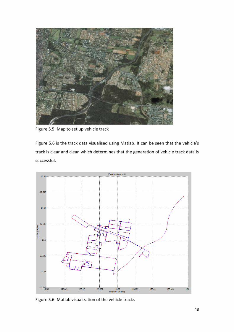
48

Figure 5.5: Map to set up vehicle track

Figure 5.6 is the track data visualised using Matlab. It can be seen that the vehicle’s

track is clear and clean which determines that the generation of vehicle track data is

successful.

Figure 5.6: Matlab visualization of the vehicle tracks

49

5.4 Case Studies of GNSS and RSU signal availability

Before performing the simulations for a well understanding of the impact of RSUs

signals on vehicle positioning performance, it is necessary to examine the availability

of GNSS and RSU signals in different cases.

Case 1: Both GPS and RSU signals are fully available

Figure 5.7 shows the case that the system is operational under the condition that

GPS signals are fully available and DSRC devices are well deployed. In this case, the

number of GPS satellites is more than that minimally required. This ensures that the

vehicles obtain accurate absolute positions using satellite positioning technology.

RSU-OBU links between vehicle and vehicle or vehicle and roadside unit are well

established, and this allows cooperative positioning services to amend the

coordinates based on other vehicle’s coordinates or the known, accurate coordinates

of roadside units.

OBU

RSU

GPS Satellite 1


GPS Satellite 4

OBU

V2V

V2RV2R

A B

Figure 5.7: Both GPS and RSU signals are fully available

50

Case 2: GPS signals are partially unavailable and RSU-OBU links are available

This refers to the case where some signals from the GPS satellites are blocked by

infrastructures. Figure 5.8 shows one of the cases under which some of the GPS

satellite signals are unavailable for vehicle A due to the blockages of infrastructures.

OBU

RSU

GPS Satellite 1


GPS Satellite 4

OBU

V2V

V2RV2R

A B

Figure 5.8: The case when GPS signals are partially unavailable

In this circumstance, vehicle A may not be able to view enough number of satellites

in order to obtain its own absolute position. Road side units and reference vehicles

need to be used in this case to calculate either the absolute or relative position using

distances between other vehicles or roadside units using specific positioning

algorithms described previously in the Chapter 4.

Case 3: OBU links are unavailable.

When vehicles are far away from each other, data links between vehicles using V2V

communication cannot be established. Figure 5.9 demonstrates the situation in

which V2R links are the only choice. As this case normally happens in open and low-

rise areas such as highways and villages, the availability of GPS satellites signals is

high, and the positioning without OBU should not introduce a big impact on

solutions.

51

OBU

RSU

GPS Satellite 1


GPS Satellite 4

OBU

V2RV2R

A B

Figure 5.9: The case when OBU links are unavailable

Case 4: GPS signals are entirely unavailable.

When vehicles are driving through tunnels or other high density areas, GPS signals

will no longer be available for positioning. In this case as shown in Figure 5.10,

communication via RSU becomes the only way for vehicles to determine their

positions.

OBU

RSU

GPS Satellite 1


GPS Satellite 4

OBU

V2V

V2RV2R

A B

Figure 5.10: GPS signals are completely unavailable

52

It is unlikely that absolute positions will be obtained without a dense layout of RSUs,

the relative positions will be determined instead. Assuming the coordinates of

roadside units are well known and accurate, the absolute positions may still be able

to be calculated using the “Estimation Algorithms” which have been shown in

previous sections.

5.5 Computational scenarios

Based on Table 2.2 and case studies of GNSS and RSU signal availability, Table 5.1

summarises the computation schemes of the simulation in order to provide a

complete picture about the performance benefits of roadside wireless infrastructure.

There are a total of 131 computing scenarios. As the most important aspect of

vehicle position is their horizontal accuracy, which may directly affect the driving

safety, the statistical results about horizontal positioning errors are used to

characterise the performance of the scenarios.

Table 5.1: Computation schemes of simulation

GNSS Mask Angle In degree

GNSS Measurement STD in meter

RSU/OBU Wireless distance STD in meter

Number of Computing scenarios

1 GPS 15,30,45 1.0,0.5,0.25 9

2 GPS+RSU 15,30,45 1.0,0.5,0.25 1.0,0.5,0.25 27

3 GPS+RSU+OBU 15,30,45 1.0,0.5,0.25 1.0,0.5,0.25 27

4 GNSS 15,30,45 1.0,0.5,0.25 9

5 GNSS+RSU 15,30,45 1.0,0.5,0.25 1.0,0.5,0.25 27

6 GNSS+RSU+OBU 15,30,45 1.0,0.5,0.25 1.0,0.5,0.25 27

7 RSU+OBU (in tunnel)

1.0,0.5,0.25,

0.15,0.1 5

Total 131

53

6 Experimental results

In this section, the simulation results with the computational schemes outlined in

Table 5.1 are presented and analysed. All these results are based on the AVG

(average) and STD (standard deviation) value of 23000 single point positioning

errors.

Figure 6.1 plots horizontal errors of three solutions: GPS only, GPS+RSU and

GPS+RSU+OBU. In this figure, the black line illustrates the vehicle route; the blue line

illustrates the GPS satellite based positioning solution which is inaccurate; the red

and magenta lines illustrate the GPS+RSU and GPS+RSU+OBU solutions. It is clear

that the fluctuation of magenta line is smaller than the blue line, which means the

accuracy is improved with wireless measurements between RSUs and OBUs. It is

worthwhile to mention that the coordinates of the other vehicle used in this

simulation are calculated using GPS/GNSS + RSU mode and are not accurate.

Figure 6.1: Illustration of positioning solutions from GPS only, GPS+RSU and

GPS+RSU+OBU

54

In the rest of the chapter, we present the simulation results from GPS and GNSS

schemes 1 and 4 as bench mark solutions respectively, where GNSS is the dual

constellations, representing GPS and Galileo for instance. Next, we examine the

simulation results from the schemes 2 and 3, GPS+RSU, and GPS+RSU+OBU, in

comparison to the schemes 4 and 5. This is followed by the analysis to the case of

RSU+OBU only in the tunnel environment. Finally, all these results under different

circumstances will be analysed and the comments will be made based on the

analysis of these results.

6.1 DGPS/GNSS solutions with the noise STD of 1, 0.5, and 0.25m

Figure 6.2a shows the horizontal STD values with GPS only under three different

mask angles and measurement STD values, while Figure 6.2b shows the STD values

of the same schemes but with dual constellations. It is clearly observed that in the

open roads, smoothed DGPS alone can marginally meet the sub-meter positioning

accuracy. With dual constellations, smoothed differential GNSS can more

comfortably meet the sub-meter requirement, with the STD value of about 0.20

meters. When in the slightly restricted roads where the average mask angle is 30

degrees, the STD values can retain in the level of several tens of centimetres. In the

restricted areas, only smooth differential GNSS can marginally achieve sub-meter

STD value with 6 to 8 high-elevation satellites in view.

Figure 6.2a: Comparison of the STD value for GPS only positioning.

1.393 1.657

5.460

0.697 0.829

2.730

0.348 0.414

1.365

0.000

1.000

2.000

3.000

4.000

5.000

6.000

Mask Angle = 15 Mask Angle = 30 Mask Angle = 45

Acc

ura

cy (

m)

GPS sigma=1

GPS sigma=0.5

GPS sigma=0.25

55

Figure 6.2b: STD values for GNSS only solutions

6.2 DGPS+RSU solutions with the noise STD of 1, 0.5, and 0.25m

For mask angle of 15 degrees, Figure 6.3a plots the HDOP values of the satellite-

based positioning and DGPS+RSU positioning against the number of satellites in view

and the number of RSU in use. Figure 6.3b compares the STD values achieved with

different mask angles and noise STD of 1, 0.5 and 0.25 meters. It shows a slight

improvement due to the distance measurements from 1 or 2 RSU. Referring to

Figure 6.3a, the improvement apparently is most likely brought by the improvement

of HDOP. The improvement is no longer obvious when the noise STD is improved to

0.5 meters or better. This indicates that the key for sub-meter positioning solutions

is the reduction of measurement noise level.

Figures 6.4a and 6.4b give the similar information when the mask angle is equal to 30

degrees while Figure 6.5a and 6.5b show the situations for the mask angle of 45

degrees.

0.770

1.275

2.162

0.385

0.638

1.081

0.192 0.319

0.540

0.000

0.500

1.000

1.500

2.000

2.500

Mask Angle = 15 Mask Angle = 30 Mask Angle = 45

Acc

ura

cy (

m)

GNSS sigma=1

GNSS sigma=0.5

GNSS sigma=0.25

56


HDOP when mask angle = 15

Figure 6.3b: STD value of GPS and GPS+RSUs positioning accuracy when mask angle = 15

Figure 6.4a and Figure 6.4b show the similar information for the case of mask angle

of 30 degrees. The number of available satellites drops to 5 at the most of the time.

The related HDOP values raise and fluctuate after RSUs are implemented. It is seen

1.393

0.697

0.348

1.128

0.637

0.339

0.983

0.564 0.319

0.901

0.491

0.282

0.000

0.200

0.400

0.600

0.800

1.000

1.200

1.400

1.600

GPS sigma=1 GPS sigma=0.5 GPS sigma=0.25

Acc

ura

cy (

m)

GPS Only

RSU Sigma=1

RSU Sigma=0.5

RSU Sigma=0.25

57

that though more apparent improvement is shown on position STD when the

measurement noise STD =1 m, it is no longer the case when the noise STD is reduced

to 0.25 meters.



Figure 6.4b: STD value of GPS and GPS+RSUs positioning accuracy when mask angle = 30

1.657

0.829

0.414

1.319

0.744

0.400

1.186

0.660 0.372

1.126

0.593

0.330

0.000

0.200

0.400

0.600

0.800

1.000

1.200

1.400

1.600

1.800


Acc

ura

cy (

m)

GPS Only

RSU Sigma=1

RSU Sigma=0.5

RSU Sigma=0.25

58



Figure 6.5b: STD value of GPS and GPS+RSU with the mask angle of 45 degrees and the number of available satellites is more than or equals to 4

As shown in Figure 6.5a, and 6.5b, the improvement in HDOP values due to the RSU

in high-mask angles is more significant. It is noticed that the HDOP value increase

5.460

2.730

1.365 2.423

1.412

0.879

2.254

1.212

0.706

2.199

1.127

0.606

0.000

1.000

2.000

3.000

4.000

5.000

6.000


Acc

ura

cy (

m)

GPS Only

RSU Sigma=1

RSU Sigma=0.5

RSU Sigma=0.25

59

dramatically in the last 2 minutes because the number of satellites (decreased to 3

now) is not sufficient for positioning any more. It is also observed that with RSU

measurements, the position STD values remain over 1 meter when the mask angle is

set 45 degrees and the number of satellites in view is 4 or more. For the case of

visible satellites are 3 or less, Figure 6.5c gives the position STD values. It is clear

that the usual deployment of RSUs does not provide sufficient improvement to the

position STD to the sub-meter accuracy, although the improvement is much more

significant with respect to the GPS only. The best results appear when both GPS and

RSU sigma is equal to 0.25, which reaches STD value of 3.34m accuracy.

Figure 6.5c: STD value of GPS+RSU solutions with the mask angle = 45 and the number of satellites is 3 or less

6.3 GPS+RSU+OBU with the measurement STD of 1m, 0.5m and 0.25m

We now wish to examine the difference that the additional measurements between

running vehicle can make to the improvement of positioning accuracy. Figure 6.6a

illustrates the available GPS satellites, its HDOP values, the number of RSUs + OBU

and the HDOP with RSU+OBU being included when GPS mask angle is set to 15

degrees. Figure 6.6b shows the position STD values with different measurement

noise STD values taken by GPS and RSU/OBU units. Comparing with 6.3b and 6.6b, it

can be seen that under the same external environment, the positioning accuracy

13.38

11.58 11.20

9.70

6.69 5.79

8.67

4.85 3.34

0.00

2.00

4.00

6.00

8.00

10.00

12.00

14.00

16.00


Acc

ura

cy (

m)

RSU Sigma=1

RSU Sigma=0.5

RSU Sigma=0.25

60

after introducing OBU is slightly higher than the case with RSUs only. Figures 6.7a

and 6.7b, Figure 6.8a and 6.8b show the results for the mask angles of 30 and 45

degrees respectively. Again, adding OBUs indeed introduces a much larger

improvement with respect to use of RSU only, especially for mask angle of 45

degrees. It is important to mention that the location of the connecting vehicle is

assumed to be determined with the combination of GPS+RSU in the same mask

angle. From the statistical results shown in Figure 6.6b, after RSUs and OBU are

implemented, the improvement in the positioning accuracy reaches maximally 65%,

65%, and 64% respectively with respect to that of the case of GPS only. It is also seen

that the RSU measurement STD is not the main factor of influence anymore,

especially when GPS STD equals to 1. The rise of accuracy is very slight when the

RSU/OBU STD value decreases from 1 to 0.5, and 0.25.The accuracy improvements

increase only by 3%, and 1% respectively.

Figure 6.6a: The relationship between the available GPS satellites, available RSUs,

and HDOP when mask angle = 15

61

Figure 6.6b: STD value of the GPS+RSUs+OBUs solutions when mask angle = 15

Figure 6.7a: Available GPS satellites, available RSUs+OBUs and HDOP when mask

angle = 30

1.393

0.697

0.348

1.059

0.616

0.335

0.904

0.529

0.308

0.847

0.452

0.265

0.000

0.200

0.400

0.600

0.800

1.000

1.200

1.400

1.600


Acc

ura

cy (

m)

GPS Only

RSU Sigma=1

RSU Sigma=0.5

RSU Sigma=0.25

62

Figure 6.7b: STD value of the GPS and the GPS+RSUs+OBUs positioning solutions when mask angle = 30

Figure 6.8a: The relationship between the available GPS satellites, available

RSUs+OBUs (refs), and HDOP when mask angle = 45

1.657

0.829

0.414

1.229

0.713

0.393

1.092

0.614

0.356

1.093

0.546

0.307

0.000

0.200

0.400

0.600

0.800

1.000

1.200

1.400

1.600

1.800


Acc

ura

cy (

m)

GPS Only

RSU Sigma=1

RSU Sigma=0.5

RSU Sigma=0.25

63

Figure 6.8b: STD value of GPS and GPS+RSUs+OBUs positioning solutions when mask angle = 45 and the number of available satellites is more than or equals to 4

Figure 6.8c: STD value of GPS and GPS+RSU+OBU solutions when mask angle = 45 and the number of available satellites is 3 or less

Figure 6.8c gives the statistical STD results of GPS+RSUs+OBU solutions when the

number of available satellites is less than the minimum requirement. It shows that

when both RSU and OBUs are introduced, the position STD values are not necessarily

reduced, but increased. For instance, when GPS STD=0.5 m or 0.25 m, and RSU/OBU

STD values are 1, 0.5 and 0.25 m, the position STD increases. This may be caused by

the poor positioning accuracy of the associated other vehicle as a mobile reference

station whose position is determined by GPS+RSU.

5.460

2.730

1.365 1.956

1.193 0.789

1.901

0.982

0.596

1.887

0.952

0.490

0.000

1.000

2.000

3.000

4.000

5.000

6.000


Acc

ura

cy (

m)

GPS Only

RSU Sigma=1

RSU Sigma=0.5

RSU Sigma=0.25

20.16

6.66

2.67

21.30

9.53

2.89

17.04

10.56

4.49 0.00

5.00

10.00

15.00

20.00

25.00


Acc

ura

cy (

m)

RSU Sigma=1

RSU Sigma=0.5

RSU Sigma=0.25

64

6.4 GNSS +RSUs with the noise STD of 1m, 0.5 m and 0.25 m

When the dual-constellation is used as GNSS in this work, the satellites in view would

roughly double. This can be expected for the future. We now examine in this case

whether RSU’s contribution is still needed. For the mask angle of 15 degrees, Figure

6.9a illustrates the number of visible satellites, available RSUs and HDOP values,

while Figure 6.9b shows the horizontal STD to the level of a few decimetres when

GNSS noise STD is 0.25m. Comparing to Figure 6.3b, the position STD value from

GNSS+RSUs are improved to about 30%.

Figure 6.9a: GNSS satellites in view, available RSUs, and HDOP when mask angle = 15

65

Figure 6.9b: STD value of the GNSS+RSUs solutions with the mask angle = 15

In the case with the mask angle of 30 degrees, Figure 6.10a and 6.10b also show the

slight improvement due to RSU measurements in HDOP and in position STD. It is

noticed that the horizontal STD remains in the level of decimetres when GNSS noise

STD is 0.25m.



0.770

0.385

0.192

0.697

0.373

0.191

0.615

0.348

0.186

0.543

0.307

0.174

0.000

0.100

0.200

0.300

0.400

0.500

0.600

0.700

0.800

0.900

GNSS sigma=1 GNSS sigma=0.5 GNSS sigma=0.25

Acc

ura

cy (

m)

GNSS Only

RSU Sigma=1

RSU Sigma=0.5

RSU Sigma=0.25

66

Figure 6.10b: STD value of GNSS+RSUs schemes when mask angle = 30

The similar results for the mask angle of 45 degrees are shown in Figure 6.11a and

6.11b. The results indicated that when the GNSS STD is about 1m, use of GNSS+RSU

can still bring the large improvement on the positioning STD. When the GNSS noise

STD is improved to 0.25 m, the GNSS+RSU can provide the position STD of lower than

0.5 meters, although the contribution of RSU is no longer a standout.



1.275

0.638

0.319

1.053

0.588

0.311

0.928

0.526

0.294

0.859

0.464

0.263

0.000

0.200

0.400

0.600

0.800

1.000

1.200

1.400


Acc

ura

cy (

m)

GNSS Only

RSU Sigma=1

RSU Sigma=0.5

RSU Sigma=0.25

67

Figure 6.11b: STD value of GNSS and GNSS+RSUs positioning solutions when mask angle = 45

6.5 GNSS, RSUs and OBU with the measurement noise STD of 1, 0.5

and 0.25m

Figures 6.12a-6.12b, 6.13a-6.13b and 6.14a-6.14b demonstrate computing results for

the mark angles of 15, 30 and 45 respectively.

Figure 6.12a: Available GNSS satellites, available RSUs+OBUs (refs) and HDOP when

the mask angle = 15

2.162

1.081

0.540

1.534

0.880

0.495

1.398

0.767

0.440

1.344

0.699

0.383

0.000

0.500

1.000

1.500

2.000

2.500


Acc

ura

cy (

m)

GNSS Only

RSU Sigma=1

RSU Sigma=0.5

RSU Sigma=0.25

68

Figure 6.12b: STD value of GPS and GNSS+RSUs+OBUs solutions when the mask angle = 15

Comparing to the same three cases for GPS+RSU+OBU as given in Figures 6.6a-6.6b,

we can see the improvement to the positioning solutions due to the second

constellations. The improvement is shown as expected.

Figure 6.13a: Available GNSS satellites and RSUs+OBUs (refs) and HDOP when mask

angle = 30

0.770

0.385

0.192

0.669

0.367

0.190

0.574

0.334

0.183

0.499

0.287

0.167

0.000

0.100

0.200

0.300

0.400

0.500

0.600

0.700

0.800

0.900


Acc

ura

cy (

m)

GNSS Only

RSU Sigma=1

RSU Sigma=0.5

RSU Sigma=0.25

69

Figure 6.13b: STD value of GNSS and GNSS+RSUs+OBUs solutions when mask angle = 30

Figure 6.14a: The relationship between available GNSS satellites, available

RSUs+OBUs (Available Refs), and HDOP when mask angle = 45

1.275

0.638

0.319

0.985

0.568

0.307

0.848

0.492

0.284

0.798

0.424

0.246

0.000

0.200

0.400

0.600

0.800

1.000

1.200

1.400


Acc

ura

cy (

m)

GNSS Only

RSU Sigma=1

RSU Sigma=0.5

RSU Sigma=0.25

70

Figure 6.14b: STD value of GPS and GNSS+RSUs+OBUs positioning solutions when mask angle = 45

The key observations are the following: 1) with RSU+OBUs, sub-meter accuracy can

be achieved when the vehicles travel through highly restricted areas, where the

average elevation angle is 45 degrees or lower; 2) Use of OBU indeed helps improve

the horizontal positioning accuracy. This improvement is more significant when the

GNSS STD noise is high, and brought through improvement to geometry.

6.6 RSUs + OBU with measurement noise STD of 1, 0.5, 0.25, 0.15, and

0.1m

Figures 6.15 and 6.16 demonstrate computing results for a tunnel case. The

deployment of RSUs is referred to in Figure 5.4. Comparing with the results based on

different noise sigmas, it can be seen that in order to reach sub-meter accuracy

positioning, the accuracy of distance measurement must be better than 0.15m. In

addition, comparing between Figures 6.15 and 6.16, we can see the improvement to

the positioning solutions due to the known height when the noise STD is higher. The

improvement is insignificant if the noise STD is comparatively low.

2.162

1.081

0.540

1.391

0.824

0.478

1.256

0.695

0.412

1.316

0.629

0.348

0.000

0.500

1.000

1.500

2.000

2.500


Acc

ura

cy (

m)

GNSS Only

RSU Sigma=1

RSU Sigma=0.5

RSU Sigma=0.25

71

Figure 6.15: STD value of RSU and RSU+OBU with unknown height data positioning

accuracy in Tunnel

Figure 6.16: STD value of RSU and RSU+OBU positioning solutions with known height

in Tunnel

3.473 3.495

1.737 1.747

0.868 0.866

0.521 0.516 0.347 0.343

0.000

0.500

1.000

1.500

2.000

2.500

3.000

3.500

4.000

RSU Only RSU+OBU

Acc

ura

cy (

m) RSU sigma=1

RSU sigma=0.5

RSU sigma=0.25

RSU sigma=0.15

RSU sigma=0.1

3.473 3.277

1.737 1.690

0.868 0.853

0.521 0.513 0.347 0.342

0.000

0.500

1.000

1.500

2.000

2.500

3.000

3.500

4.000

RSU Only RSU+OBU

Acc

ura

cy (

m) RSU sigma=1

RSU sigma=0.5

RSU sigma=0.25

RSU sigma=0.15

RSU sigma=0.1

72

7. Conclusions

To address the Intelligent Transport System challenges for road safety, it has been

identified that seamless, lane-level or sub-meter level vehicle positioning solutions

are essentially required. The problem is that standalone Global Positioning System

(GPS) or Differential GPS (DGPS) suffer from solution outages while being used in

restricted areas such as high-rise urban areas and tunnels, due to blockages of

satellite signals. Smoothed DGPS can provide the sub-meter positioning accuracy,

but cannot meet the seamless requirement. A disadvantage of the traditional

navigation aids such as Dead Reckoning and Inertial Measurement Unit onboard

vehicles are either not accurate enough due to error accumulation or too expensive

to be acceptable by the mass market vehicle users.

This research has explored the unification of satellite based GNSS systems and

roadside wireless infrastructure as an alternative solution through extensive

simulation studies. The thesis has reviewed the smoothed Differential GPS

techniques in both single base and network modes, which offer the ranges

measurements at the decimetre uncertainty easily. A number of wireless

infrastructures which can be potentially installed on roadsides to provide additional

distance signals, LocataLites, Dedicated Short-Range communication (DSRC) and

Ultra-Wide Broadband (UWB) are discussed and compared. Models and algorithms

have been developed to integrate GNSS and other wireless measurements. A total of

131 computational schemes were designed in the simulation studies.

Results from the above experimental schemes have confirmed the following findings:

1) In the open road areas where sufficient satellite signals can be received, the

roadside wireless measurements contribute very little to the improvement of

horizontal positioning accuracy at the sub-meter level, especially in the dual

constellation cases.

2) In the restricted or medium-rise urban environments where averagely 4 to 5

GPS satellites are visible, a set of 1 to 3 roadside and onboard distance

measurements can help improve both positioning accuracy of around 1

73

meter. This accuracy can be improved to sub-meter to decimetre levels when

dual GNSS constellations are available. Positioning accuracy improvement

using the integrated positioning solutions mainly relies on the accuracy of the

GPS/GNSS measurements.

3) When the vehicle is travelling in tunnels with known heights of tunnel

surfaces and roadside distance measurements, the sub-meter horizontal

positioning accuracy is also achievable if the roadside distance measurements

are accurate to 0.2m or better. One realistic choice of such infrastructure is

LocateLites

4) Overall, simulation results have demonstrated that roadside infrastructure,

such as LocateLites indeed has the potential to provide sub-meter vehicle

position solutions for certain road safety applications if the properly deployed

roadside measurements are obtainable.

The above findings are obtained when the RSUs distributed in regular circumstances.

More dense deployment may result in better accuracy as well. This will be the part of

future work.

The above findings are based on assumption that Locatalites or DSRC RSUs can

provide required distance measurements to high-mobility vehicles. To establish or

confirm this capability, extensive experiments in various road environments may be

conducted. Studies of using DSRC signals for positioning are still in the very early

stage.

74

References

Architecture Development Team (2007). Executive Summary. In U. D. o. Transportation (Ed.), National Intelligent Transportation System (ITS) Architecture. Washington D.C.: Research and Innovation Technology Administration (RITA).

Belanovic, P., Valerio, D., Paier, A., Zemen, T., Ricciato, F., & Mecklenbrauker, C. F. (2010). On Wireless Links for Vehicle-to-Infrastructure Communications. Vehicular Technology, IEEE Transactions on, 59(1), 269-282.

Bensky, A. (2007). Wireless Positioning Technologies and Applications: Artech House, Inc. Berder, O., Quemerais, P., Sentieys, O., Astier, J., Nguyen, T. D., Menard, J., et al. (2008, 24-

24 Oct. 2008). Cooperative communications between vehicles and intelligent road signs. Paper presented at the ITS Telecommunications, 2008. ITST 2008. 8th International Conference on.

Bishop, R. (2000a). Intelligent vehicle applications worldwide. Intelligent Systems and their Applications, IEEE, 15(1), 78-81.

Bishop, R. (2000b). A survey of intelligent vehicle applications worldwide. Paper presented at the Intelligent Vehicles Symposium, 2000. IV 2000. Proceedings of the IEEE.

Biswas, S., Tatchikou, R., & Dion, F. (2006). Vehicle-to-vehicle wireless communication protocols for enhancing highway traffic safety. Communications Magazine, IEEE, 44(1), 74-82.

Braasch, M. S. (1996, 22-26 Apr 1996). GPS multipath model validation. Paper presented at the Position Location and Navigation Symposium, 1996., IEEE 1996.

Chong, C.-C., Watanabe, F., & Inamura, H. (2006, 28-31 Aug. 2006). Potential of UWB Technology for the Next Generation Wireless Communications. Paper presented at the Spread Spectrum Techniques and Applications, 2006 IEEE Ninth International Symposium on.

Chris, A., Randolph, W., Christian, R., & John, B. (2000). Obtaining single path phase delays from GPS double differences. Geophysical Research Letters, 27, 2661-2664.

Ciurana, M., Barcelo-Arroyo, F., & Izquierdo, F. (2007, 11-15 March 2007). A Ranging Method with IEEE 802.11 Data Frames for Indoor Localization. Paper presented at the Wireless Communications and Networking Conference, 2007.WCNC 2007. IEEE.

Commonwealth of Australia (2009). Planning for intelligent transport systems - Proposals for the introduction of intelligent transport systems into the 5.9 GHz band in Australia. Canberra: Communications and Publishing Retrieved from http://www.acma.gov.au/webwr/_assets/main/lib311208/ifc27-09_intelligent_transport_systems_5.9ghz_band.pdf.

Dana, P. H. (1996). Global Positioning System Overview. Retrieved from http://www.colorado.edu/geography/gcraft/notes/gps/gps.html

Drane, C., Macnaughtan, M., & Scott, C. (1998). Positioning GSM telephones. Communications Magazine, IEEE, 36(4), 46-54, 59.

Efatmaneshnik, M., Balaei, A. T., Alam, N., & Dempster, A. G. (2009, 11-12 Nov. 2009). A modified multidimensional scaling with embedded particle filter algorithm for cooperative positioning of vehicular networks. Paper presented at the Vehicular Electronics and Safety (ICVES), 2009 IEEE International Conference on.

Fan, B., & Krishnan, H. (2006). Reliability Analysis of DSRC Wireless Communication for Vehicle Safety Applications. Paper presented at the Intelligent Transportation Systems Conference, 2006. ITSC '06. IEEE.

Federal Communications Commission. (2002). The first report and order regarding ultra-wideband transmission systems FCC 02-48.

http://www.acma.gov.au/webwr/_assets/main/lib311208/ifc27-09_intelligent_transport_systems_5.9ghz_band.pdf

http://www.acma.gov.au/webwr/_assets/main/lib311208/ifc27-09_intelligent_transport_systems_5.9ghz_band.pdf

http://www.colorado.edu/geography/gcraft/notes/gps/gps.html

75

Federal Communications Commission. (2004). Amend Rules Regarding Dedicated Short Range Communications Services and rules for Mobile Service for Dedicated Short Range Communications of Intelligent Transportation Services. Washington, D.C.

Filjar, R., Busic, L., & Kos, T. (2005, 12-14 Oct. 2005). Differential Satellite Positioning Accuracy for LBS: A Zagreb Case Study. Paper presented at the Applied Electromagnetics and Communications, 2005. ICECom 2005. 18th International Conference on.

Gaderer, G., Loschmidt, P., Nagy, A., Exel, R., & Sauter, T. (2009, 25-28 Oct. 2009). Localisation in wireless sensor networks. Paper presented at the Sensors, 2009 IEEE.

Gu, X., & Lipp, A. (1994, 11-15 Apr 1994). DGPS positioning using carrier phase for precision navigation. Paper presented at the Position Location and Navigation Symposium, 1994., IEEE.

Hatch, R. (1982). The synergism of GPS code and carrier measurements. [Proceedings]. 3rd, Las Cruces, NM, II(The synergism of GPS code and carrier measurements.), p1213-1231.

Hepsaydir, E. (1999, 1999). Mobile positioning in CDMA cellular networks. Paper presented at the Vehicular Technology Conference, 1999. VTC 1999 - Fall. IEEE VTS 50th.

Huang, J., & Tan, H. S. (2006). A Low-Order DGPS-Based Vehicle Positioning System Under Urban Environment. Mechatronics, IEEE/ASME Transactions on, 11(5), 567-575.

IEEE Computer Society. (2007). IEEE Standard for Information technology-Telecommunications and information exchange between systems-Local and metropolitan area networks-Specific requirements. IEEE Std 802.11-2007.

IEEE Standards Department. (2005). Draft STANDARD for Information technology-Telecommunications and information exchange between systems-Local and metropolitan area networks-Specific requirements-Part 11: Wireless LAN Medium Access Control (MAC) and Physical Layer (PHY) specifications Amendment 8: Wireless Network Management. IEEE Unapproved Draft Std P802.11p/D1.1, Jan 2005.

Jiang, D., & Delgrossi, L. (2008). IEEE 802.11p: Towards an International Standard for Wireless Access in Vehicular Environments. Paper presented at the Vehicular Technology Conference, 2008. VTC Spring 2008. IEEE.

Khoomboon, S., Kasetkasem, T., Keinprasit, R., & Sugino, N. (2010, 19-21 May 2010). Increase a standalone GPS positioning accuracy by using a proximity sensor. Paper presented at the Electrical Engineering/Electronics Computer Telecommunications and Information Technology (ECTI-CON), 2010 International Conference on.

Leick, A. (2003). GPS Satellite Surveying (III ed.): Wiley. Li, B., Kam, J., Lui, J., Dempster, A. G., & Rizos, C. (2007). Direction-based Wireless LAN

positioning. Paper presented at the 4th Int. Symp. on Location Based Services & TeleCartograph, Hong Kong.

Lin, T.-N., & Lin, P.-C. (2005, 13-16 June 2005). Performance comparison of indoor positioning techniques based on location fingerprinting in wireless networks. Paper presented at the Wireless Networks, Communications and Mobile Computing, 2005 International Conference on.

Liu, C., & Lo, C. (2010, 19-20 June 2010). The study for the WLAN with Bluetooth positioning system. Paper presented at the Advances in Energy Engineering (ICAEE), 2010 International Conference on.

Liu, Y., & Wang, Y. (2009, 2-4 Dec. 2009). Linear Method for WLAN Positioning System. Paper presented at the Software Engineering Research, Management and Applications, 2009. SERA '09. 7th ACIS International Conference on.

Llombart, M., Ciurana, M., & Barcelo-Arroyo, F. (2008, 27-27 March 2008). On the scalability of a novel WLAN positioning system based on time of arrival measurements. Paper

76

presented at the Positioning, Navigation and Communication, 2008. WPNC 2008. 5th Workshop on.

Mahfouz, M. R., Fathy, A. E., Kuhn, M. J., & Wang, Y. (2009, 24-25 Sept. 2009). Recent trends and advances in UWB positioning. Paper presented at the Wireless Sensing, Local Positioning, and RFID, 2009. IMWS 2009. IEEE MTT-S International Microwave Workshop on.

Mahfouz, M. R., Kuhn, M. J., To, G., & Fathy, A. E. (2009). Integration of UWB and Wireless Pressure Mapping in Surgical Navigation. Microwave Theory and Techniques, IEEE Transactions on, 57(10), 2550-2564.

Morgan, Y. (2009). Accurate positioning using Short-Range Communications. Paper presented at the Ultra Modern Telecommunications & Workshops, 2009. ICUMT '09. International Conference on.

National.Research.Council.(U.S.). (1995). The global positioning system: a shared national asset : recommendations for technical improvements and enhancement. 264.

Parker, R., & Valaee, S. (2007a, 24-28 June 2007). Cooperative Vehicle Position Estimation. Paper presented at the Communications, 2007. ICC '07. IEEE International Conference on.

Parker, R., & Valaee, S. (2007b). Vehicular Node Localization Using Received-Signal-Strength Indicator. Vehicular Technology, IEEE Transactions on, 56(6), 3371-3380.

Parkinson, B. W., & Spilker.Jr, J. J. (1996). Global Positioning System: Theory and Applications Volume II (Vol. 164). Washington: AIAA.

Patel, U. R., & Gohil, B. N. (2010, 9-11 July 2010). Cell identity assignment techniques in cellular network: A review. Paper presented at the Computer Science and Information Technology (ICCSIT), 2010 3rd IEEE International Conference on.

Peden, M. (2004). World report on road traffic injury prevention: summary. Geneva: World Health Organization.

Potgantwar, A. D., & Wadhai, V. M. (2011, 20-22 July 2011). Location Based System for Mobile Devices with Integration of RFID and Wireless Technology-Issues and Proposed System. Paper presented at the Process Automation, Control and Computing (PACC), 2011 International Conference on.

Rahayu, Y., Rahman, T. A., Ngah, R., & Hall, P. S. (2008, 5-7 May 2008). Ultra wideband technology and its applications. Paper presented at the Wireless and Optical Communications Networks, 2008. WOCN '08. 5th IFIP International Conference on.

Rizos, C., Li, Y., Politi, N., Barnes, J., & Gamble, N. (2011). Locata: A New Constellation for High Accuracy Outdoor and Indoor Positioning. Paper presented at the International Federation of Surveyors, Marrakech, Morocco.

Rizos, C., Roberts, G., Barnes, J., & Gambale, N. (2010, 15-17 Sept. 2010). Experimental results of Locata: A high accuracy indoor positioning system. Paper presented at the Indoor Positioning and Indoor Navigation (IPIN), 2010 International Conference on.

Rizos, C., Yan, T., Omar, S., Musa, T., & Kinlyside, D. (2003). Implementing netowork-RTK: the SydNET CORS infrastructure 6th Int. Symp. on Satellite Navigation Technology Including Mobile Positioning & Location Services (pp. 22-25). Melbourne.

Roberto, S., & Giovanni, B., Palmerini. (2008). Differential Global Positioning System (DGPS) for Flight Testing. Flight Test Instrumentation Series, 21.

Sadayuki, T. (2005). Issue and recent trends in vehicle safety communication systems. IATSS Res, 29(1), 7-15.

Scott, G., & Demoz, G.-E. (2009). GNSS Applications and Methods. Boston: Artech House. Son, L. T., & Orten, P. (2007, 11-15 March 2007). Enhancing Accuracy Performance of

Bluetooth Positioning. Paper presented at the Wireless Communications and Networking Conference, 2007.WCNC 2007. IEEE.

77

Tan, H. S., & Huang, J. (2006). DGPS-Based Vehicle-to-Vehicle Cooperative Collision Warning: Engineering Feasibility Viewpoints. Intelligent Transportation Systems, IEEE Transactions on, 7(4), 415-428.

Tappero, F., Merminod, B., & Ciurana, M. (2010, 15-17 Sept. 2010). IEEE 802.11 ranging and multi-lateration for software-defined positioning receiver. Paper presented at the Indoor Positioning and Indoor Navigation (IPIN), 2010 International Conference on.

Tay, B., Liu, W., & Zhang, D. H. (2009). Indoor Angle of Arrival positioning using biased estimation. Paper presented at the Industrial Informatics, 2009. INDIN 2009. 7th IEEE International Conference on.

Wright, M., Stallings, D., & Dunn, D. (2003, 4-6 April 2003). The effectiveness of global positioning system electronic navigation. Paper presented at the SoutheastCon, 2003. Proceedings. IEEE.

Xu, G. (2007). GPS : Theory, Algorithms and Applications Retrieved from http://QUT.eblib.com.au/patron/FullRecord.aspx?p=337967

Yang, L., & Giannakis, G. B. (2004). Ultra-wideband communications: an idea whose time has come. Signal Processing Magazine, IEEE, 21(6), 26-54.

Yeh, S.-C., Hsu, W.-H., Su, M.-Y., Chen, C.-H., & Liu, K.-H. (2009, 26-29 March 2009). A study on outdoor positioning technology using GPS and WiFi networks. Paper presented at the Networking, Sensing and Control, 2009. ICNSC '09. International Conference on.

Yin, H., & Alamouti, S. (2006). OFDMA: A Broadband Wireless Access Technology. Paper presented at the Sarnoff Symposium, 2006 IEEE.

Zhao, Y., Zhou, H., Li, M., & Kong, R. (2008, 12-14 Oct. 2008). Implementation of Indoor Positioning System Based on Location Fingerprinting in Wireless Networks. Paper presented at the Wireless Communications, Networking and Mobile Computing, 2008. WiCOM '08. 4th International Conference on.

http://qut.eblib.com.au/patron/FullRecord.aspx?p=337967

78

Appendix A

1. Define earth's gravitational constant

2. Define earth's rotation rate

3. Calculate semi-major axis:

4. Calculate mean motion

5. Calculate time from ephemeris reference epoch

6. Correct mean motion

7. Calculate mean anomaly

8. Solve Kepler’s equation for eccentric anomaly

9. Calculate true anomaly

10. Calculate eccentric anomaly

11. Calculate argument of latitude

12. Calculate argument of latitude correction

δ

13. Calculate radius correction

δ

14. Calculate inclination correction

79

δ

15. Calculate the corrected argument of latitude

δ

16. Calculate corrected radius

δ

17. Calculate corrected inclination

δ

18. Calculate positions in orbital plane

19. Calculate corrected longitude of ascending node

20. Calculate Earth-fixed coordinates

80

Appendix B

Table 0.1: PDOP, HDOP, and 2D accuracy AVG and STD values of GPS only positioning.

Mask Angle Num of Sats DSRC sigma GPS sigma PDOP HDOP 2D

15 7 1 1 2.895 2.432 0.003 AVG

0.306 0.279 1.393 STD

7 1 0.5 2.895 2.432 0.002 AVG

0.306 0.279 0.697 STD

7 1 0.25 2.895 2.432 0.001 AVG

0.306 0.279 0.348 STD

7 0.5 1 2.895 2.432 0.003 AVG

0.306 0.279 1.393 STD

7 0.5 0.5 2.895 2.432 0.002 AVG

0.306 0.279 0.697 STD

7 0.5 0.25 2.895 2.432 0.001 AVG

0.306 0.279 0.348 STD

7 0.25 1 2.895 2.432 0.003 AVG

0.306 0.279 1.393 STD

7 0.25 0.5 2.895 2.432 0.002 AVG

0.306 0.279 0.697 STD

7 0.25 0.25 2.895 2.432 0.001 AVG

0.306 0.279 0.348 STD

30 5 1 1 4.043 3.384 0.005 AVG

0.273 0.222 1.657 STD

5 1 0.5 4.043 3.384 0.002 AVG

0.273 0.222 0.829 STD

5 1 0.25 4.043 3.384 0.001 AVG

0.273 0.222 0.414 STD

5 0.5 1 4.043 3.384 0.005 AVG

0.273 0.222 1.657 STD

5 0.5 0.5 4.043 3.384 0.002 AVG

0.273 0.222 0.829 STD

5 0.5 0.25 4.043 3.384 0.001 AVG

0.273 0.222 0.414 STD

5 0.25 1 4.043 3.384 0.005 AVG

0.273 0.222 1.657 STD

5 0.25 0.5 4.043 3.384 0.002 AVG

0.273 0.222 0.829 STD

5 0.25 0.25 4.043 3.384 0.001 AVG

0.273 0.222 0.414 STD

45 4 1 1 15.541 12.007 0.081 AVG

1.977 0.660 5.460 STD

4 1 0.5 15.541 12.007 0.041 AVG

1.977 0.660 2.730 STD

4 1 0.25 15.541 12.007 0.020 AVG

1.977 0.660 1.365 STD

4 0.5 1 15.541 12.007 0.081 AVG

1.977 0.660 5.460 STD

4 0.5 0.5 15.541 12.007 0.041 AVG

1.977 0.660 2.730 STD

4 0.5 0.25 15.541 12.007 0.020 AVG

1.977 0.660 1.365 STD

4 0.25 1 15.541 12.007 0.081 AVG

1.977 0.660 5.460 STD

4 0.25 0.5 15.541 12.007 0.041 AVG

1.977 0.660 2.730 STD

4 0.25 0.25 15.541 12.007 0.020 AVG

1.977 0.660 1.365 STD

81

Table 0.2: PDOP, HDOP, and 2D accuracy AVG and STD values of GPS+RSU positioning.


15 7 1 1 2.313 1.946 0.004 AVG

0.396 0.374 1.128 STD

7 1 0.5 2.313 1.946 0.003 AVG

0.396 0.374 0.637 STD

7 1 0.25 2.313 1.946 0.001 AVG

0.396 0.374 0.339 STD

7 0.5 1 2.313 1.946 0.002 AVG

0.396 0.374 0.983 STD

7 0.5 0.5 2.313 1.946 0.002 AVG

0.396 0.374 0.564 STD

7 0.5 0.25 2.313 1.946 0.001 AVG

0.396 0.374 0.319 STD

7 0.25 1 2.313 1.946 0.001 AVG

0.396 0.374 0.901 STD

7 0.25 0.5 2.313 1.946 0.001 AVG

0.396 0.374 0.491 STD

7 0.25 0.25 2.313 1.946 0.001 AVG

0.396 0.374 0.282 STD

30 5 1 1 3.116 2.623 0.005 AVG

0.573 0.526 1.319 STD

5 1 0.5 3.116 2.623 0.003 AVG

0.573 0.526 0.744 STD

5 1 0.25 3.116 2.623 0.001 AVG

0.573 0.526 0.400 STD

5 0.5 1 3.116 2.623 0.005 AVG

0.573 0.526 1.186 STD

5 0.5 0.5 3.116 2.623 0.003 AVG

0.573 0.526 0.660 STD

5 0.5 0.25 3.116 2.623 0.001 AVG

0.573 0.526 0.372 STD

5 0.25 1 3.116 2.623 0.005 AVG

0.573 0.526 1.126 STD

5 0.25 0.5 3.116 2.623 0.003 AVG

0.573 0.526 0.593 STD

5 0.25 0.25 3.116 2.623 0.001 AVG

0.573 0.526 0.330 STD

45 4 1 1 5.855 4.746 0.018 AVG

3.415 2.561 2.423 STD

4 1 0.5 5.855 4.746 0.012 AVG

3.415 2.561 1.412 STD

4 1 0.25 5.855 4.746 0.010 AVG

3.415 2.561 0.879 STD

4 0.5 1 5.855 4.746 0.016 AVG

3.415 2.561 2.254 STD

4 0.5 0.5 5.855 4.746 0.009 AVG

3.415 2.561 1.212 STD

4 0.5 0.25 5.855 4.746 0.006 AVG

3.415 2.561 0.706 STD

4 0.25 1 5.855 4.746 0.016 AVG

3.415 2.561 2.199 STD

4 0.25 0.5 5.855 4.746 0.008 AVG

3.415 2.561 1.127 STD

4 0.25 0.25 5.855 4.746 0.004 AVG

3.415 2.561 0.606 STD

82

Table 0.3: PDOP, HDOP, and 2D accuracy AVG and STD values of GPS+RSU+OBU positioning.


15 7 1 1 2.187 1.846 0.001 AVG

0.362 0.341 1.059 STD

7 1 0.5 2.189 1.847 0.001 AVG

0.362 0.341 0.616 STD

7 1 0.25 2.189 1.847 0.001 AVG

0.362 0.341 0.335 STD

7 0.5 1 2.188 1.846 0.003 AVG

0.362 0.341 0.904 STD

7 0.5 0.5 2.189 1.847 0.001 AVG

0.362 0.341 0.529 STD

7 0.5 0.25 2.189 1.847 0.001 AVG

0.362 0.341 0.308 STD

7 0.25 1 2.188 1.847 0.003 AVG

0.362 0.341 0.847 STD

7 0.25 0.5 2.189 1.847 0.002 AVG

0.362 0.341 0.452 STD

7 0.25 0.25 2.189 1.847 0.000 AVG

0.362 0.341 0.265 STD

30 5 1 1 2.970 2.518 0.004 AVG

0.575 0.519 1.229 STD

5 1 0.5 2.975 2.522 0.003 AVG

0.575 0.519 0.713 STD

5 1 0.25 2.977 2.524 0.002 AVG

0.575 0.519 0.393 STD

5 0.5 1 2.972 2.520 0.005 AVG

0.575 0.518 1.092 STD

5 0.5 0.5 2.976 2.523 0.002 AVG

0.575 0.519 0.614 STD

5 0.5 0.25 2.977 2.524 0.001 AVG

0.575 0.519 0.356 STD

5 0.25 1 2.973 2.521 0.005 AVG

0.575 0.519 1.093 STD

5 0.25 0.5 2.976 2.524 0.002 AVG

0.575 0.519 0.546 STD

5 0.25 0.25 2.977 2.524 0.001 AVG

0.575 0.519 0.307 STD

45 4 1 1 4.435 3.697 0.007 AVG

1.799 1.424 1.956 STD

4 1 0.5 4.472 3.728 0.006 AVG

1.794 1.419 1.193 STD

4 1 0.25 4.490 3.743 0.008 AVG

1.797 1.421 0.789 STD

4 0.5 1 4.444 3.705 0.010 AVG

1.792 1.420 1.901 STD

4 0.5 0.5 4.479 3.734 0.004 AVG

1.790 1.416 0.982 STD

4 0.5 0.25 4.493 3.746 0.004 AVG

1.793 1.418 0.596 STD

4 0.25 1 4.449 3.709 0.021 AVG

1.791 1.420 1.887 STD

4 0.25 0.5 4.483 3.737 0.005 AVG

1.789 1.416 0.952 STD

4 0.25 0.25 4.495 3.748 0.002 AVG

1.792 1.417 0.490 STD

83

Table 0.4: PDOP, HDOP, and 2D accuracy AVG and STD values of GPS only positioning when available satellites equals to 3.


45 3 1 1 45475700 39240812 17538.25 AVG

58543904 50520399 0.569234 STD

3 1 0.5 45475700 39240812 17538.25 AVG

58543904 50520399 0.569234 STD

3 1 0.25 45475700 39240812 17538.25 AVG

58543904 50520399 0.569234 STD

3 0.5 1 45475700 39240812 17538.25 AVG

58543904 50520399 0.569234 STD

3 0.5 0.5 45475700 39240812 17538.25 AVG

58543904 50520399 0.569234 STD

3 0.5 0.25 45475700 39240812 17538.25 AVG

58543904 50520399 0.569234 STD

3 0.25 1 45475700 39240812 17538.25 AVG

58543904 50520399 0.569234 STD

3 0.25 0.5 45475700 39240812 17538.25 AVG

58543904 50520399 0.569234 STD

3 0.25 0.25 45475700 39240812 17538.25 AVG

58543904 50520399 0.569234 STD

84

Table 0.5: PDOP, HDOP, and 2D accuracy AVG and STD values of GPS+RSU positioning when available satellites equals to 3.


45 3 1 1 26.27903 22.79468 0.948226 AVG

275.3784 237.7507 13.37675 STD

3 1 0.5 26.27903 22.79468 0.828302 AVG

275.3784 237.7507 11.58479 STD

3 1 0.25 26.27903 22.79468 0.769203 AVG

275.3784 237.7507 11.1971 STD

3 0.5 1 26.27903 22.79468 0.598311 AVG

275.3784 237.7507 9.700605 STD

3 0.5 0.5 26.27903 22.79468 0.474113 AVG

275.3784 237.7507 6.688373 STD

3 0.5 0.25 26.27903 22.79468 0.414151 AVG

275.3784 237.7507 5.792394 STD

3 0.25 1 26.27903 22.79468 0.425318 AVG

275.3784 237.7507 8.673132 STD

3 0.25 0.5 26.27903 22.79468 0.299155 AVG

275.3784 237.7507 4.850303 STD

3 0.25 0.25 26.27903 22.79468 0.237056 AVG

275.3784 237.7507 3.344187 STD

85

Table 0.6: PDOP, HDOP, and 2D accuracy AVG and STD values of GPS+RSU+OBU positioning when available satellites equals to 3.


45 3 1 1 4.820713 4.209684 1.229037 AVG

1.30502 1.052424 20.1619 STD

3 1 0.5 4.836175 4.220011 0.313721 AVG

1.248844 1.005584 6.658315 STD

3 1 0.25 4.845247 4.226275 0.02947 AVG

1.228566 0.989353 2.668877 STD

3 0.5 1 4.854723 4.236128 1.690585 AVG

1.296871 1.044121 21.30475 STD

3 0.5 0.5 4.873856 4.249583 0.649979 AVG

1.247044 1.00335 9.529183 STD

3 0.5 0.25 4.891355 4.262481 0.17714 AVG

1.22948 0.989714 2.886771 STD

3 0.25 1 4.869721 4.247784 2.248608 AVG

1.297134 1.043624 17.03676 STD

3 0.25 0.5 4.886271 4.25872 0.880402 AVG

1.25155 1.00549 10.55502 STD

3 0.25 0.25 4.906071 4.273402 0.331348 AVG

1.233347 0.992058 4.494865 STD

86

Table 0.7: PDOP, HDOP, and 2D accuracy AVG and STD values of GNSS only positioning.


15 16 1 1 1.502 1.336 0.003 AVG

0.094 0.100 0.770 STD

16 1 0.5 1.502 1.336 0.002 AVG

0.094 0.100 0.385 STD

16 1 0.25 1.502 1.336 0.001 AVG

0.094 0.100 0.192 STD

16 0.5 1 1.502 1.336 0.003 AVG

0.094 0.100 0.770 STD

16 0.5 0.5 1.502 1.336 0.002 AVG

0.094 0.100 0.385 STD

16 0.5 0.25 1.502 1.336 0.001 AVG

0.094 0.100 0.192 STD

16 0.25 1 1.502 1.336 0.003 AVG

0.094 0.100 0.770 STD

16 0.25 0.5 1.502 1.336 0.002 AVG

0.094 0.100 0.385 STD

16 0.25 0.25 1.502 1.336 0.001 AVG

0.094 0.100 0.192 STD

30 10 1 1 2.855 2.474 0.003 AVG

0.263 0.355 1.275 STD

10 1 0.5 2.855 2.474 0.002 AVG

0.263 0.355 0.638 STD

10 1 0.25 2.855 2.474 0.001 AVG

0.263 0.355 0.319 STD

10 0.5 1 2.855 2.474 0.003 AVG

0.263 0.355 1.275 STD

10 0.5 0.5 2.855 2.474 0.002 AVG

0.263 0.355 0.638 STD

10 0.5 0.25 2.855 2.474 0.001 AVG

0.263 0.355 0.319 STD

10 0.25 1 2.855 2.474 0.003 AVG

0.263 0.355 1.275 STD

10 0.25 0.5 2.855 2.474 0.002 AVG

0.263 0.355 0.638 STD

10 0.25 0.25 2.855 2.474 0.001 AVG

0.263 0.355 0.319 STD

45 8 1 1 6.072 4.773 0.015 AVG

0.207 0.256 2.162 STD

8 1 0.5 6.072 4.773 0.008 AVG

0.207 0.256 1.081 STD

8 1 0.25 6.072 4.773 0.004 AVG

0.207 0.256 0.540 STD

8 0.5 1 6.072 4.773 0.015 AVG

0.207 0.256 2.162 STD

8 0.5 0.5 6.072 4.773 0.008 AVG

0.207 0.256 1.081 STD

8 0.5 0.25 6.072 4.773 0.004 AVG

0.207 0.256 0.540 STD

8 0.25 1 6.072 4.773 0.015 AVG

0.207 0.256 2.162 STD

8 0.25 0.5 6.072 4.773 0.008 AVG

0.207 0.256 1.081 STD

8 0.25 0.25 6.072 4.773 0.004 AVG

0.207 0.256 0.540 STD

87

Table 0.8: PDOP, HDOP, and 2D accuracy AVG and STD values of GNSS+RSU positioning.


15 16 1 1 1.379 1.218 0.002 AVG

0.118 0.127 0.697 STD

16 1 0.5 1.379 1.218 0.001 AVG

0.118 0.127 0.373 STD

16 1 0.25 1.379 1.218 0.001 AVG

0.118 0.127 0.191 STD

16 0.5 1 1.379 1.218 0.002 AVG

0.118 0.127 0.615 STD

16 0.5 0.5 1.379 1.218 0.001 AVG

0.118 0.127 0.348 STD

16 0.5 0.25 1.379 1.218 0.001 AVG

0.118 0.127 0.186 STD

16 0.25 1 1.379 1.218 0.002 AVG

0.118 0.127 0.543 STD

16 0.25 0.5 1.379 1.218 0.001 AVG

0.118 0.127 0.307 STD

16 0.25 0.25 1.379 1.218 0.001 AVG

0.118 0.127 0.174 STD

30 10 1 1 2.355 2.031 0.002 AVG

0.336 0.356 1.053 STD

10 1 0.5 2.355 2.031 0.001 AVG

0.336 0.356 0.588 STD

10 1 0.25 2.355 2.031 0.001 AVG

0.336 0.356 0.311 STD

10 0.5 1 2.355 2.031 0.002 AVG

0.336 0.356 0.928 STD

10 0.5 0.5 2.355 2.031 0.001 AVG

0.336 0.356 0.526 STD

10 0.5 0.25 2.355 2.031 0.000 AVG

0.336 0.356 0.294 STD

10 0.25 1 2.355 2.031 0.003 AVG

0.336 0.356 0.859 STD

10 0.25 0.5 2.355 2.031 0.001 AVG

0.336 0.356 0.464 STD

10 0.25 0.25 2.355 2.031 0.000 AVG

0.336 0.356 0.263 STD

45 8 1 1 3.991 3.260 0.009 AVG

1.073 0.819 1.534 STD

8 1 0.5 3.991 3.260 0.007 AVG

1.073 0.819 0.880 STD

8 1 0.25 3.991 3.260 0.004 AVG

1.073 0.819 0.495 STD

8 0.5 1 3.991 3.260 0.007 AVG

1.073 0.819 1.398 STD

8 0.5 0.5 3.991 3.260 0.005 AVG

1.073 0.819 0.767 STD

8 0.5 0.25 3.991 3.260 0.003 AVG

1.073 0.819 0.440 STD

8 0.25 1 3.991 3.260 0.007 AVG

1.073 0.819 1.344 STD

8 0.25 0.5 3.991 3.260 0.004 AVG

1.073 0.819 0.699 STD

8 0.25 0.25 3.991 3.260 0.002 AVG

1.073 0.819 0.383 STD

88

Table 0.9: PDOP, HDOP, and 2D accuracy AVG and STD values of GNSS+RSU+OBU positioning.


15 16 1 1 1.356 1.198 0.002 AVG

0.117 0.123 0.669 STD

16 1 0.5 1.356 1.198 0.001 AVG

0.117 0.123 0.367 STD

16 1 0.25 1.356 1.198 0.001 AVG

0.117 0.123 0.190 STD

16 0.5 1 1.356 1.198 0.002 AVG

0.117 0.123 0.574 STD

16 0.5 0.5 1.356 1.198 0.001 AVG

0.117 0.123 0.334 STD

16 0.5 0.25 1.356 1.198 0.001 AVG

0.117 0.123 0.183 STD

16 0.25 1 1.356 1.198 0.002 AVG

0.117 0.123 0.499 STD

16 0.25 0.5 1.356 1.198 0.001 AVG

0.117 0.123 0.287 STD

16 0.25 0.25 1.356 1.198 0.001 AVG

0.117 0.123 0.167 STD

30 10 1 1 2.272 1.967 0.003 AVG

0.321 0.324 0.985 STD

10 1 0.5 2.273 1.968 0.001 AVG

0.321 0.324 0.568 STD

10 1 0.25 2.274 1.969 0.001 AVG

0.321 0.324 0.307 STD

10 0.5 1 2.272 1.967 0.003 AVG

0.321 0.324 0.848 STD

10 0.5 0.5 2.273 1.968 0.001 AVG

0.321 0.324 0.492 STD

10 0.5 0.25 2.274 1.969 0.001 AVG

0.321 0.324 0.284 STD

10 0.25 1 2.273 1.968 0.003 AVG

0.321 0.324 0.798 STD

10 0.25 0.5 2.274 1.968 0.001 AVG

0.321 0.324 0.424 STD

10 0.25 0.25 2.274 1.969 0.001 AVG

0.321 0.324 0.246 STD

45 8 1 1 3.649 3.040 0.014 AVG

0.940 0.765 1.391 STD

8 1 0.5 3.661 3.051 0.009 AVG

0.940 0.765 0.824 STD

8 1 0.25 3.667 3.056 0.005 AVG

0.940 0.766 0.478 STD

8 0.5 1 3.654 3.044 0.011 AVG

0.939 0.764 1.256 STD

8 0.5 0.5 3.664 3.053 0.007 AVG

0.940 0.765 0.695 STD

8 0.5 0.25 3.667 3.056 0.004 AVG

0.940 0.766 0.412 STD

8 0.25 1 3.655 3.046 0.012 AVG

0.939 0.764 1.316 STD

8 0.25 0.5 3.665 3.054 0.006 AVG

0.940 0.765 0.629 STD

8 0.25 0.25 3.668 3.057 0.004 AVG

0.940 0.766 0.348 STD

A simulation study of Unified GPS and Roadside Ranging Technologies...

Documents

Transcript of A simulation study of Unified GPS and Roadside Ranging Technologies...