A Simulation Study of the Effect of Powerful High ... · A Simulation Study of the Effect of...

World Journal of Research and Review (WJRR)

ISSN:2455-3956, Volume-3, Issue-5, November 2016 Pages 01-09

1 www.wjrr.org

A Simulation Study of the Effect of Powerful High-

Frequency Radio Waves on the Behavior of Super-

Small-Scale Irregularities in the F-layer Ionospheric

Plasma

O.V. Mingalev, M.N. Melnik, V.S. Mingalev

Abstract - Magnetic field aligned super-small-scale

irregularities in the concentration of charged particles are

often observed in the Earth’s ionosphere and magnetosphere.

Earlier, the time evolution of such irregularities was studied

with the help of the mathematical model, developed in the

Polar Geophysical Institute. This model is based on a

numerical solution of the Vlasov-Poisson system of equations.

This mathematical model is used in the present paper. The

purpose of the present paper is to examine numerically how

high-power high-frequency radio waves, utilized for artificial

heating experiments and pumped into the ionosphere by

ground-based ionospheric heaters, influence on the time

evolution of the super-small-scale irregularities present

naturally in the F-layer ionospheric plasma. The results of

simulation indicate that a presence of high-power high-

frequency radio wave ought to influence essentially on the

behavior of physically significant parameters of the plasma

inside and in the vicinity of the irregularity.

Index Terms - ionospheric plasma, super-small-scale

irregularities, numerical simulation.

I. INTRODUCTION

In the Earth’s ionosphere, electron density irregularities are

present always. Spatial sizes of these irregularities can vary

from thousands of kilometers to a few centimeters. The

electron density depletions and increases inside

irregularities can lie in the range from a few portions to

some tens of percentages. Various types of irregularities

can exist in the ionosphere, in particular, large-scale

irregularities in the ionospheric F layer [1]-[6], middle-

scale irregularities [7]-[8], short-scale irregularities [9]-

[14], and super-small-scale irregularities [15]. It is known

that not large-scale irregularities are predominately

magnetic field aligned.

The electron density irregularities in the ionosphere

can be formed not only by natural physical processes but

also as a result of active experiments. In particular,

ionospheric irregularities may be formed by high-power

high-frequency radio waves, pumped into the ionosphere

by ground based ionospheric heaters [15]-[19]. These

waves can cause a variety of physical processes in the

ionospheric plasma.

O.V. Mingalev, Polar Geophysical Institute, Russian Academy of

Sciences, Apatity, Murmansk Region, Russia.

M.N. Melnik, Polar Geophysical Institute, Russian Academy of Sciences,

Apatity, Murmansk Region, Russia.

V.S. Mingalev, Polar Geophysical Institute, Russian Academy of

Sciences, Apatity, Murmansk Region, Russia.

This work was partly supported by the Division of the Physical Sciences

of the Russian Academy of Sciences through the program “Dynamics of

rarefied plasma in space and laboratory”.

These processes can result in the formation of not only

large-scale irregularities in the electron temperature and

electron concentration but also super-small-scale

irregularities in the concentration of charged particles.

For investigation of the behavior of the artificially

created irregularities in the ionospheric plasma not only the

experimental and theoretical but also computational studies

may be applied. The formation of large-scale irregularities

by powerful high frequency waves, utilized for artificial

heating experiments and pumped into the ionosphere by

ground-based ionospheric heaters, was investigated with

the help of mathematical models in some studies (for

example, see [16-29]). The formation of the super-small-

scale irregularities in the concentration of charged particles

in the F-layer ionosphere by powerful high frequency

waves was considered and simulated in the study by

Eliasson and Stenflo [30]. It should be emphasized that

such irregularities may be formed in the ionospheric plasma

not only artificially but also by natural processes [15].

The time evolution of super-small-scale irregularities

was investigated with the help of the mathematical model,

developed in the Polar Geophysical Institute, under natural

conditions without action of powerful high frequency

waves in studies [31]-[33]. It may be expected that

powerful high frequency waves can influence on the

behavior of existent super-small-scale irregularities.

In the present study, the mathematical model,

developed earlier in the Polar Geophysical Institute, is

utilized for numerical investigation of the effect of high-

power high-frequency radio waves on the time evolution of

the super-small-scale irregularities, created naturally in the

F-layer ionospheric plasma. The present work is the

continuation of the investigation begun in the study of

Mingalev et al. [33], with new simulation results being

submitted in the present paper.

II. MATHEMATICAL MODEL

To examine numerically how high-power high-frequency

radio waves, pumped into the ionosphere by ground-based

ionospheric heaters, influence on the time evolution of the

super-small-scale irregularities, present naturally in the F-

layer ionospheric plasma, the mathematical model,

developed earlier in the Polar Geophysical Institute [33], is

utilized. This model is based on a numerical solution of the

Vlasov-Poisson system of equations.

At F-layer altitudes, the ionospheric plasma is

supposed to be a rarefied compound consisting of electrons

and positive ions in the presence of a strong, external,

uniform magnetic field. The studied irregularities are

A Simulation Study of the Effect of Powerful High-Frequency Radio Waves on the Behavior of Super-Small-Scale

Irregularities in the F-layer Ionospheric Plasma

2 www.wjrr.org

geomagnetic field-aligned, with their cross-sections being

circular. The initial cross-section diameters of the

irregularities are supposed to be several Debye lengths (no

more than about 100) [15].

At F-layer levels, the mean free path of particles

(electrons and ions) between successive collisions is much

more than the cross-section diameters of the considered

irregularities. Therefore, the plasma is assumed to be

collisionless. Kinetic processes in such plasma are

described by the Vlasov-Poisson system of equations which

has been considered, for example, in the studies by

Hockney and Eastwood [34], and Birdsall and Langdon

[35]. This system may be written as follows:

0

, , 0,a a a a

a

f f q f

t m

v E v Bx v

, ,a i e

(1)

0

1, , ,t t

Δ x x (2)

, , ,t t E x x

0

, , , , , ,i e a a

t e n n n t f t d x x x v v

where ( , , )a

f t x v , ( , ), ,a a

n t mx and a

q are, respectively,

the distribution function, concentration, mass, and charge

of particles of type a , x is the space coordinate vector, v

is the velocity, 0

B is the external magnetic field, E is the

self-consistent electric field, , t x is the electric field

potential, , t x is the electric charge density, 0 is the

dielectric constant of free space, and 0e is the proton

charge. The Vlasov kinetic equation (1) describes the

evolution of the distribution functions of charged particles

and the Poisson equation (2) describes the self-consistent

electric field.

It may be recalled that the investigated irregularities

are geomagnetic field-aligned. Their longitudinal sizes are

much more than the cross-section diameters. Gradients of

the plasma parameters in the longitudinal direction are

much less than those in a plane perpendicular to a magnetic

field in the vicinity of the irregularity. Therefore, plasma

parameters in the vicinity of the irregularity may be

considered as independent on the longitudinal coordinate.

This simplification allow us to consider a two dimensional

flow of plasma in a plane perpendicular to a magnetic field

line. Therefore, the mathematical model, developed earlier

in the Polar Geophysical Institute and utilized in [31]-[33],

is two-dimensional. This mathematical model is used in the

present study, too.

A macroparticle method is utilized for numerical

solving of the Vlasov equations (1). A finite-difference

method is used for numerical solving of the Poisson

equation (2). In the applied version of the mathematical

model a motion of the positive ions is taken into account. In

the model calculations, a two-dimensional simulation

region, lain in the plane perpendicular to the magnetic field

line, is a square and its side length is equal to 128 Debye

lengths of the plasma. The quantity of the grid cells is

1024×1024 and the average number of macro-particles in

the Debye cell for the model plasma is 215. Detailed

description of the utilized mathematical model may be

found in the study of Mingalev et al. [33].

III. PRESENTATION AND DISCUSSION OF

RESULTS

Calculations with the help of the utilized two-dimensional

mathematical model can be made for various conditions in

the ionospheric plasma. The results of calculations to be

presented in this paper were obtained using the input

parameters of the model typical for the nocturnal F-layer

ionospheric plasma at the level of 300 km. At this level, the

plasma, apart from electrons, contains positive ions, with

the oxygen ion, O+, being the bulk of ion content (99%).

The value of the non-disturbed electron concentration

(equal to the positive ion concentration), n0 , is 1011 m-3.

The electron and ion temperatures are supposed to be equal

to 1213 K and 930 K, respectively. At the initial moment,

the bulk flow velocities of electrons and positive ions, ue

and ui respectively, are assumed to be zero. The value of

the magnetic field, 0B , is 4.4∙105

T.

Under chosen conditions in the ionospheric plasma, the

equilibrium plasma frequency, ω0pe, is 1.78∙107 s-1, the

frequency of cyclotron oscillations of electrons, ωce, is

7.74∙106 s-1, the Debye length of the plasma, 0λDe , is equal

to 7.6∙10-3 m, the equilibrium period of Langmuir

oscillations of electrons, Tpe, is 3.52∙10-7 s, the equilibrium

period of Langmuir oscillations of oxygen ions, Tpi, is

approximately a factor of 171 larger than the equilibrium

period of Langmuir oscillations of electrons (Tpi ≈ 171∙Tpe),

the period of cyclotron oscillations of electrons, Tce, is

approximately a factor of 2.3 larger than the equilibrium

period of Langmuir oscillations of electrons (Tce ≈ 2.3∙Tpe),

and the mean free time of electron between successive

collisions with other particles is larger than the equilibrium

period of Langmuir oscillations of electrons by a factor of

about 1047.

The simulation results to be presented in this paper

were obtained for the following initial state of the

irregularity inside the two-dimensional simulation region.

The spatial distribution of the electron concentration (equal

to the positive ion concentration at the initial moment),

contains a circular irregularity at the center of the

simulation region. Beyond this irregularity, the electron

concentration is homogeneous and coincides with the non-

disturbed electron concentration, n0. The initially created

irregularity has the cross-section diameter of 120λDe . Inside

the irregularity, homogeneity of the plasma is broken and a

part of charged particles travels from the internal circle,

having the diameter of 60λDe , into the external ring,

surrounding the internal circle. The relative decrease of the

concentration of charged particles, (n0 – ne)/n0 , is equal to

0.1 in the internal circle at the initial moment, that is, 10

percent of charged particles were displaced from the center

of the irregularity to its periphery, with the plasma having

been electrically neutral at the initial moment.

We have calculated the time evolution of the

distribution functions of charged particles as well as self-

consisting electric field for two distinct on principle

situations. The first situation corresponds to absence of

external electric field, whereas the second situation

corresponds to presence of external electric field which



3 www.wjrr.org

represents a high-power high-frequency radio wave,

pumped into the ionosphere by a ground-based ionospheric

heater. It is supposed that this radio wave illuminates the

two-dimensional simulation region.

Fig 1: The calculated spatial distributions of the normalized

electric charge density, (ni – ne) / n0 , in the plane

perpendicular to the magnetic field. The vector of the

magnetic field lies on the axis, perpendicular to the

simulation region, and is directed downwards. The

normalized distances, X /0λDe and Y /

0λDe , that is, the

distances in units of the Debye length, 0λDe , from the

central point of the simulation region are shown on the

horizontal (X) and vertical (Y) axes. For the first situation,

correspondent to absence of an external electric field, the

results are presented in the left column, whereas, for the

second situation, correspondent to presence of the high-

power high-frequency radio wave, the results are shown in

the right column. The results are given for the following

moments: t = 5.2∙Tpe (top panel), t = 25∙Tpe (middle panel),

t = 100∙Tpe (bottom panel).

In the second situation, the high-frequency radio wave,

radiated by a ground-based ionospheric heater, is supposed

to propagate along a magnetic field line up to the reflection

point, to turn back, and to propagate towards the Earth’s

surface along a magnetic field line, with the disturbing high-

frequency radio wave becoming a standing wave. It may be

noted that the described situation can be more probably

realized at high latitudes where the direction of magnetic

field is close to vertical.

As was noted earlier, the two-dimensional simulation

region lies in the plane perpendicular to the magnetic field

line. Therefore, the vector of the high-frequency wave’s

electric field, E, lies in the plane of the simulation region

and has not a projection perpendicular to the simulation

region. It is assumed that the disturbing high-frequency

radio wave is ordinary and that its frequency, ω0, is equal to

the frequency of the electron hybrid resonance, namely, ω0

= [(ω0pe)

2 + (ωce)2]1/2. It turns out that the frequency of the

disturbing high-frequency radio wave is approximately a

factor of 1.09 larger than the equilibrium plasma frequency

(ω0 ≈ 1.09∙ω0pe). After the initial moment, the module of the

vector of the high-frequency wave’s electric field increases

smoothly and, during the time interval of five periods of

Langmuir oscillations of electrons, reaches the value of 0.49

V/m which is quite attainable, for example, for the heating

facility near Tromso, Scandinavia. The vector of the high-

frequency wave’s electric field, E, rotates with the

frequency equal to ω0 in each point of the two-dimensional

simulation region.

Simulation results, obtained for the first situation,

correspondent to absence of an external electric field,

indicate that, after initial moment, the spatial distribution of

the electron concentration changes essentially while the

positive ion concentration is retained practically invariable.

It turns out that the initially created irregularity vanishes

completely during a short period, with the plasma becoming

electrically neutral in all simulation region at the moment

near to the equilibrium period of Langmuir oscillations of

electrons .pe

t T Further calculations indicate that the

changes in the electron concentration are continued and,

after a short period, the irregularity arises again to a moment

of about (2.2 2.3) ,pe

T with the recovered irregularity

almost completely coinciding with the initial one. Later, the

cycle of vanishing and recovering of the irregularity is

repeated again and again. Thus, the time evolution of the

initially created irregularity is accompanied by periodic

vibrations. The period of these vibrations is approximately a

factor of 2.3 larger than the equilibrium period of Langmuir

oscillations of electrons, with the former period coinciding

with the period of cyclotron oscillations of electrons, .ce

T In

the course of time, the amplitudes of the vibrations of the

electron concentration decrease smoothly, with the

irregularity decaying little by little.

In the process of evolution, additional almost

symmetrical alternate rings with an excess of charge of

different sign begin to appear around the initial irregularity

situated in the center of the simulation region. In the course

of time, these additional rings begin to fill up all simulation

region, with the irregularity center remaining immovable.

It is of interest to note that, in the process of evolution,

essential electric fields can arise at the points of the

simulation region situated between the rings with an excess

of charge of different sign, in particular, close to the center

of the simulation region where the initially created

irregularity has been situated.

Simulation results, obtained for the second situation,

correspondent to presence of the high-power high-

frequency radio wave, have both distinctions and common

features with the results, obtained for the first situation

correspondent to absence of external electric field.

The spatial distributions of the normalized electric

charge density, calculated for some moments, are presented

in Figure 1. It is seen that the results, obtained for two

considered situations, have some common features. The



4 www.wjrr.org

irregularities vanish and recover periodically, with its parameters fluctuating.

Fig 2: The time variations of one component of the electric field, namely Ex , lying in the plane perpendicular to the

magnetic field, calculated at the point, displaced from the center of the simulation region in the X direction for a distance

of three Debye lengths 03 λDe . For the first situation, correspondent to absence of an external electric field, the

results are shown by blue line, whereas, for the second situation, correspondent to presence of the high-power high-

frequency radio wave, the results are shown by red line. The electric field component is given in V/m. The normalized

time, t /peT , that is, the time in units of the equilibrium period of Langmuir oscillations of electrons,

peT , is shown on the

abscissa.

Fig 3: The time variations of one component of the electric field, namely Ey , lying in the plane perpendicular to the


of three Debye lengths 03 λDe . For the first situation, correspondent to absence of an external electric field, the





5 www.wjrr.org



abscissa.

Fig 4: The time variations of one component of the electric field, namely Ex , lying in the plane perpendicular to the


of sixteen Debye lengths 016 λDe . For the first situation, correspondent to absence of an external electric field, the





abscissa.

Fig 5: The time variations of one component of the electric field, namely Ey , lying in the plane perpendicular to the


of sixteen Debye lengths 016 λDe . For the first situation, correspondent to absence of an external electric field, the





6 www.wjrr.org



abscissa.

Fig 6: The spatial distributions of the vector of the bulk flow velocity of electrons, ue, calculated for the second situation,

correspondent to presence of the high-power high-frequency radio wave, in the plane perpendicular to the magnetic field.

The normalized distances, X /0λDe and Y /

0λDe , that is, the distances in units of the Debye length, 0λDe , from the central

point of the simulation region are shown on the horizontal (X) and vertical (Y) axes. The vector of the magnetic field lies on

the axis, perpendicular to the simulation region, and is directed downwards. The colouration of the figures indicates the

module of the velocity in km/s. The results are given for the following moments: (a) t = 98.6∙Tpe, (b) t = 99∙Tpe, (c) t =

99.4∙Tpe, (d) t = 99.8∙Tpe.

Examples of fluctuating parameters of the plasma are

presented in Figures 2-5 where time variations of the

electric field components at two points of the simulation

region are shown. It is seen that the amplitudes of the

electric field fluctuations, obtained for the second situation,

correspondent to presence of the high-power high-

frequency radio wave, are much more than those, obtained

for the first situation, correspondent to absence of external

electric field. The former amplitudes are close to the

module of the vector of the external high-frequency wave’s

electric field (0.49 V/m).

Other distinction between the results, obtained for two

considered situations, concerns the periods of the

fluctuations. For the first situation, correspondent to

absence of an external electric field, it is easy to see from

Figures 2-5 that the electric field fluctuations posses of two

main periods, namely, the period of Langmuir oscillation of

electrons and period of cyclotron oscillations of electrons.

In particular, the period of the fluctuations, having maximal

amplitudes, is close to the period of cyclotron oscillations

of electrons, which is approximately a factor of 2.3 larger

than the period of Langmuir oscillations of electrons.

Unlike, for the second situation, correspondent to presence

of the high-power high-frequency radio wave, the period of

the electric field fluctuations is close to the period of the

vibrations of the disturbing high-frequency radio wave. The

later period is approximately a factor of 0.92 smaller than

the equilibrium period of Langmuir oscillations of

electrons.

It is known that the ionospheric plasma at F-layer

altitudes is strongly magnetized. As a consequence, the

bulk flow velocities of electrons and positive ions, ue and ui

respectively, in the direction perpendicular to the magnetic

field B is strongly affected by the electric field E, with the



7 www.wjrr.org

plasma transport perpendicular to the magnetic field lines

following EB direction. As was noted earlier, the vector

of the high-power high-frequency wave’s electric field, E,

rotates in each point of the two-dimensional simulation

region. Therefore, the bulk flow velocities of electrons and

positive ions, ue and ui respectively, ought to rotate, too.

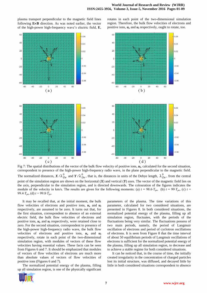
Fig 7: The spatial distributions of the vector of the bulk flow velocity of positive ions, ui, calculated for the second situation,

correspondent to presence of the high-power high-frequency radio wave, in the plane perpendicular to the magnetic field.

The normalized distances, X /0λDe and Y /

0λDe , that is, the distances in units of the Debye length, 0λDe , from the central

point of the simulation region are shown on the horizontal (X) and vertical (Y) axes. The vector of the magnetic field lies on

the axis, perpendicular to the simulation region, and is directed downwards. The colouration of the figures indicates the

module of the velocity in km/s. The results are given for the following moments: (a) t = 98.6∙Tpe, (b) t = 99∙Tpe, (c) t =

99.4∙Tpe, (d) t = 99.8∙Tpe.

It may be recalled that, at the initial moment, the bulk

flow velocities of electrons and positive ions, ue and ui

respectively, are assumed to be zero. It turns out that, for

the first situation, correspondent to absence of an external

electric field, the bulk flow velocities of electrons and

positive ions, ue and ui respectively, were retained close to

zero. For the second situation, correspondent to presence of

the high-power high-frequency radio wave, the bulk flow

velocities of electrons and positive ions, ue and ui

respectively, rotate in each point of the two-dimensional

simulation region, with modules of vectors of these flow

velocities having essential values. These facts can be seen

from Figures 6 and 7. It should be emphasized that modules

of vectors of flow velocities of electrons are much more

than absolute values of vectors of flow velocities of

positive ions (Figures 6 and 7).

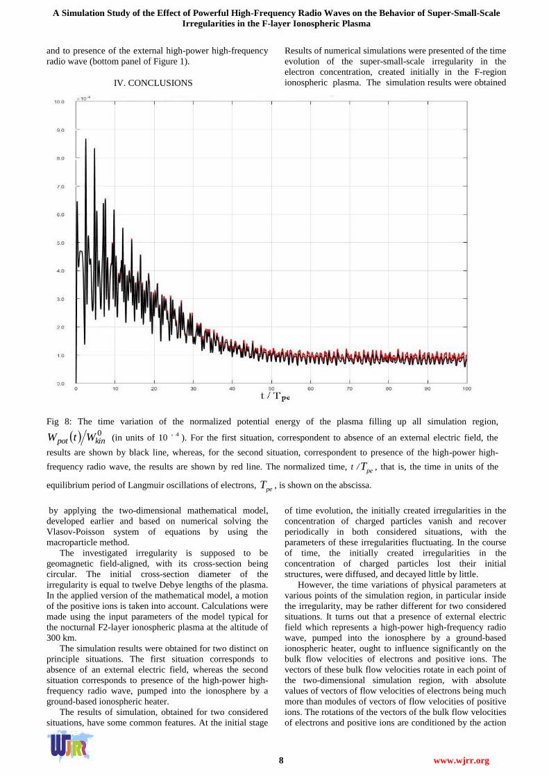
The normalized potential energy of the plasma, filling

up all simulation region, is one of the physically significant

parameters of the plasma. The time variations of this

parameter, calculated for two considered situations, are

presented in Figures 8. In both considered situations, the

normalized potential energy of the plasma, filling up all

simulation region, fluctuates, with the periods of the

fluctuations being very similar. The fluctuations possess of

two main periods, namely, the period of Langmuir

oscillation of electrons and period of cyclotron oscillations

of electrons. It is seen from Figure 8 that the time interval

of about 50 equilibrium periods of Langmuir oscillations of

electrons is sufficient for the normalized potential energy of

the plasma, filling up all simulation region, to decrease and

to achieve a stable regime for both considered situations.

It can be noticed that, in the course of time, the initially

created irregularity in the concentration of charged particles

lost its initial structure, was diffused, and decayed little by

little in both considered situations correspondent to absence



8 www.wjrr.org

and to presence of the external high-power high-frequency

radio wave (bottom panel of Figure 1).

IV. CONCLUSIONS

Results of numerical simulations were presented of the time

evolution of the super-small-scale irregularity in the

electron concentration, created initially in the F-region

ionospheric plasma. The simulation results were obtained

Fig 8: The time variation of the normalized potential energy of the plasma filling up all simulation region,

0kinpot WtW (in units of 10 - 4 ). For the first situation, correspondent to absence of an external electric field, the

results are shown by black line, whereas, for the second situation, correspondent to presence of the high-power high-

frequency radio wave, the results are shown by red line. The normalized time, t /peT , that is, the time in units of the

equilibrium period of Langmuir oscillations of electrons, peT , is shown on the abscissa.

by applying the two-dimensional mathematical model,

developed earlier and based on numerical solving the

Vlasov-Poisson system of equations by using the

macroparticle method.

The investigated irregularity is supposed to be

geomagnetic field-aligned, with its cross-section being

circular. The initial cross-section diameter of the

irregularity is equal to twelve Debye lengths of the plasma.

In the applied version of the mathematical model, a motion

of the positive ions is taken into account. Calculations were

made using the input parameters of the model typical for

the nocturnal F2-layer ionospheric plasma at the altitude of

300 km.

The simulation results were obtained for two distinct on

principle situations. The first situation corresponds to

absence of an external electric field, whereas the second

situation corresponds to presence of the high-power high-

frequency radio wave, pumped into the ionosphere by a

ground-based ionospheric heater.

The results of simulation, obtained for two considered

situations, have some common features. At the initial stage

of time evolution, the initially created irregularities in the

concentration of charged particles vanish and recover

periodically in both considered situations, with the

parameters of these irregularities fluctuating. In the course

of time, the initially created irregularities in the

concentration of charged particles lost their initial

structures, were diffused, and decayed little by little.

However, the time variations of physical parameters at

various points of the simulation region, in particular inside

the irregularity, may be rather different for two considered

situations. It turns out that a presence of external electric

field which represents a high-power high-frequency radio

wave, pumped into the ionosphere by a ground-based

ionospheric heater, ought to influence significantly on the

bulk flow velocities of electrons and positive ions. The

vectors of these bulk flow velocities rotate in each point of

the two-dimensional simulation region, with absolute

values of vectors of flow velocities of electrons being much

more than modules of vectors of flow velocities of positive

ions. The rotations of the vectors of the bulk flow velocities

of electrons and positive ions are conditioned by the action



9 www.wjrr.org

of the rotating vector of the high-frequency wave’s electric

field.

ACKNOWLEDGMENT

The authors would like to thank the Editor and the

anonymous referees for their careful reading and

benevolent evaluation.

REFERENCES

[1] Moffet, R. J. and Quegan, S. (1983) The mid-latitude through in the

electron concentration of the ionospheric F-layer: a review of

observations and modelling. Journal of Atmospheric and Terrestrial

Physics, 45, 315-343.

[2] Buchau, J., Reinisch, B. W., Weber, E. T., and Moore, J. G. (1983)

Structure and dynamics of the winter polar cap F region. Radio

Science, 18, 995-1010.

[3] Robinson, R. W., Tsunoda, R. T., Vickrey, J. F., and Guerin, L. (1985)

Sources of F region ionization enhancement in the nighttime auroral

zone. Journal of Geophysical Research, 90, 7533-7546.

[4] Ivanov-Kholodny, G.S., Goncharova, E.E., Shashun’kina, V.M., and

Yudovich, L.A. (1987) Daily variations in the zonal structure of the

ionospheric F region at low latitudes in February 1980.

Geomagnetism and Aeronomia, 27(5), 722-727 (Russian issue).

[5] Tsunoda, R. T. (1988) High-latitude F region irregularities: A review

and synthesis. Review of Geophysics, 26, 719-760.

[6] Besprozvannaya, A.S., Zherebtsov, G.A., Pirog, O.M., and Shchuka,

T.I. (1988) Dynamics of electron density in the auroral zone during

the magnetospheric substorm on December 22, 1982. Geomagnetism

and Aeronomia, 28 (1), 66-70 (Russian issue).

[7] Muldrew, D. B. and Vickrey, J. F. (1982) High-latitude F region

irregularities observed simultaneously with ISIS1 and Chatanika

radar. Journal of Geophysical Research, 87 (A10), 8263-8272.

[8] Basu, S., Mac Kenzie, E., Basu, S., Fougere, P. F., Maynard, N. C.,

Coley, W. R., Hanson, W. B., Winningham, J. D., Sugiura, M., and

Hoegy, W. R. (1988) Simultaneous density and electric field

fluctuation spectra associated with velocity shears in the auroral

oval. Journal of Geophysical Research, 93 (A1), 115-136.

[9] Martin, E. and Aarons, J. (1977) F layer scintillations and the aurora.

Journal of Geophysical Research, 82, 2717-2722.

[10] Fremouw, E. J., Rino C. L., Livingston R. C., and Cousins M. C.

(1977) A persistent subauroral scintillations enhancement observed

in Alaska. Geophysical Research Letters, 4, 539-542.

[11] Kersley, L., Russell, C. D., and Pryse S. E. (1989) Scintillation and

EISCAT investigations of gradient-drift irregularities in the high

latitude ionosphere. Journal of Atmospheric and Terrestrial Physics,

51, 241-247.

[12] Pryse, S. E., Kersley, L., and Russell, C. D. (1991) Scintillation near

the F layer trough over northern Europe. Radio Science, 26, 1105-

1114.

[13] Greenwald, R.A. (1974) Diffuse radar aurora and the gradient drift

instability. Journal of Geophysical Research, 79, 4807-4810.

[14] Dimant, Ya. S., Oppenheim, M. M., and Milikh, G. M. (2009) Meteor

plasma trails: effects of external electric field. Annales Geophysicae,

27, 279-296.

[15] Wong, A. Y., Santoru, J., Darrow, C., Wang, L., and Roederer, J.G.

(1983) Ionospheric cavitons and related nonlinear phenomena. Radio

Science, 18, 815-830.

[16] Meltz, G. and LeLevier, R.E. (1970) Heating the F-region by

deviative absorption of radio waves. Journal of Geophysical

Research, 75, 6406-6416.

[17] Perkins, F.W. and Roble, R.G. (1978) Ionospheric heating by radio

waves: Predictions for Arecibo and the satellite power station.

Journal of Geophysical Research, 83 (A4), 1611-1624.

[18] Mantas, G.P., Carlson, H.C., and La Hoz, C.H. (1981) Thermal

response of F-region ionosphere in artificial modification

experiments by HF radio waves. Journal of Geophysical Research,

86 (A2), 561-574.

[19] Bernhardt, P.A. and Duncan, L.M. (1982) The feedback-diffraction

theory of ionospheric heating. Journal of Atmospheric and

Terrestrial Physics, 44, 1061-1074.

[20] Hansen, J.D., Morales, G.J., and Maggs, J.E. (1989) Daytime

saturation of thermal cavitons. Journal of Geophysical Research, 94

(A6), 6833-6840.

[21] Vas’kov, V.V., Dimant, Ya.S., and Ryabova, N.A. (1993)

Magnetospheric plasma thermal perturbations induced by resonant

heating of the ionospheric F-region by high-power radio wave.

Advances in Space Research, 13 (10), 25-33.

[22] Mingaleva, G.I. and Mingalev, V.S. (1997) Response of the

convecting high-latitude F layer to a powerful HF wave, Annales

Geophysicae, 15, 1291-1300.

[23] Mingaleva, G.I. and Mingalev, V.S. (2002) Modeling the

modification of the nighttime high-latitude F region by powerful HF

radio waves. Cosmic Research, 40 (1), 55-61.

[24] Mingaleva, G.I. and Mingalev, V.S. (2003) Simulation of the

modification of the nocturnal high-latitude F layer by powerful HF

radio waves. Geomagnetism and Aeronomy, 43 (6), 816-825

(Russian issue).

[25] Mingaleva, G.I., Mingalev, V.S., and Mingalev, I.V. (2003)

Simulation study of the high-latitude F-layer modification by

powerful HF waves with different frequencies for autumn conditions.

Annales Geophysicae, 21, 1827-1838.

[26] Mingaleva, G.I., Mingalev, V.S., and Mingalev, I.V. (2009) Model

simulation of the large-scale high-latitude F-layer modification by

powerful HF waves with different modulation. Journal of

Atmospheric and Solar-Terrestrial Physics, 71, 559-568.

[27] Mingaleva, G.I., Mingalev, V.S., and Mingalev, O.V. (2012)

Simulation study of the large-scale modification of the mid-latitude

F-layer by HF radio waves with different powers. Annales

Geophysicae, 30, 1213–1222, doi:10.5194/angeo-30-1213-2012.

[28] Mingaleva, G.I. and Mingalev, V.S. (2013) Simulation study of the

modification of the high-latitude ionosphere by powerful high-

frequency radio waves. Journal of Computations and Modelling,

3(4), 287-309.

[29] Mingaleva G.I. and Mingalev V.S. (2014) Model simulation of

artificial heating of the daytime high-latitude F-region ionosphere by

powerful high-frequency radio waves // International Journal of

Geosciences, Volume 2014(5), 363-374.

[30] Eliasson, B. and Stenflo, L. (2008) Full-scale simulation study of the

initial stage of ionospheric turbulence. Journal of Geophysical

Research, 113 (A2), A02305.

[31] Mingalev, O.V., Mingalev, I. V., and Mingalev, V. S. (2006) Two-

dimensional numerical simulation of dynamics of small-scale

irregularities in the near-Earth plasma. Cosmic Research, 44 (5),

398-408.

[32] Mingalev, O.V., Mingaleva, G. I., Melnik, M.N., and Mingalev, V. S.

(2010) Numerical modeling of the behavior of super-small-scale

irregularities in the ionospheric F2 layer. Geomagnetism and

Aeronomy, 50(5), 643-654.

[33] Mingalev O.V., Melnik M.N., Mingalev V.S. Numerical modeling of

the time evolution of super-small-scale irregularities in the near-

Earth rarefied plasma // International Journal of Geosciences.-2015.-

V. 6. P. 67-78.

[34] Hockney, R.W. and Eastwood, J.W. (1981) Computer simulation

using particles. McGraw-Hill. New York.

[35] Birdsall, C.K. and Langdon, A.B. (1985) Plasma physics via

computer simulation. McGraw-Hill. New York.

http://adsabs.harvard.edu/cgi-bin/author_form?author=Dimant,+Y&fullauthor=Dimant,%20Y.%20S.&charset=ISO-8859-1&db_key=PHY

http://adsabs.harvard.edu/cgi-bin/author_form?author=Oppenheim,+M&fullauthor=Oppenheim,%20M.%20M.&charset=ISO-8859-1&db_key=PHY

http://adsabs.harvard.edu/cgi-bin/author_form?author=Milikh,+G&fullauthor=Milikh,%20G.%20M.&charset=ISO-8859-1&db_key=PHY

A Simulation Study of the Effect of Powerful High ... · A Simulation Study of the Effect of...

Documents

Transcript of A Simulation Study of the Effect of Powerful High ... · A Simulation Study of the Effect of...