A Simplified Plasma Current Profile Model for Tokamak Control

E. Witrant, S. Bremond, F. Delebecque and J.-P. Quadrat

Abstract— The purpose of this paper is to present a sim-plified model of the current and temperature dynamics oftokamak plasma. It is focused on the diffusion behaviorsand relates the profiles of physical variables to engineeringcontrol inputs. The Scilab/Scicos environment is used for thenumerical implementation of this model. This work is a firststep towards the control of the current profile.

I. INTRODUCTION

A tokamak is a physical device in which a plasmais confined using magnetic coils set in the poloidal andtoroidal planes (see Figure 1). The plasma behaves as aconductor that is heated by the current induced by thevariation of the magnetic flux in the ohmic coils. Thetokamak can then be considered, in a first approximation, asa large transformer where the current of the secondary coilsis used to heat the primary coil. As the plasma resistivityis decreasing with temperature, it is also necessary to addother heating sources that enhance the plasma confinment(confinment of the energy at the center of the plasma) andincrease the overall temperature. This is done thanks toradio-frequency antennas (such as the lower hybrid oneconsidered in this work) that allow to reach a very highcentral temperature, which is necessary to obtain fusionreactions.

Plasma

Toroidal field coil

Poloidal field coil

Ohmic field coil

Fig. 1. Tokamak.

E. Witrant is with KTH, Osquldas vag 10, SE-100 44 Stockholm(Sweden).S. Bremond is with CEA/DSM/DRFC, CEA/Cadarache, 13108 ST PAULLEZ DURANCE CEDEX (France).F. Delebecque and J.P. Quadrat are with Inria-Rocquencourt, Meta-lau Project, Domaine de Voluceau, 78150 Le CHESNAY (France).Email:Francois.Delebecque@inria.fr

The control of tokamak plasma has a long history (see[3]-[4]). In particular, four classes of control problems havebeen investigated:

• vertical stabilization of the plasma center,• control of the magnetic surfaces shape,• control of mangnetohydrodynamic (MHD) instabili-

ties,• control of the current, temperature and density profiles.

We are concerned with the last problem, which has beenstudied more recently in [6], [5], [7]. The goal is to providefor the operating conditions (in terms of profiles shapes)that are necessary to achieve advanced confinment schemesand increase the fusion power production efficiency. Forexample, the so called H-mode is characterized by a trans-port barrier located at the plasma edge, which improves theconfinment, and will be the operating mode of the futureITER tokamak.The previous profile control approaches cited above aremainly based on black box linear models and plasmaphysics are only used to select the set of relevant variablesand the way they are coupled. These approaches implythe identification of a MIMO system approximating adistributed system and are highly dependant on the op-erating conditions, which makes them costly in terms ofexperimentations. The aim of this paper is then to providefor a control-oriented model established with a nonlinearsystem of PDE based on:

• the evolution of the resistive equation averaged on themagnetic surface as explained in [1],

• the experimental identification of some diffusion coef-ficients.

The control problem is formulated and the model givingthe current density is numerically solved in the Scilab-Scicos environment. Based on some experimental data, thesimulation results provided by the proposed model are ingood agreement with those obtained by the Cronos software.Cronos is one of the references to study the transport equa-tions in tokamak plasmas and includes complex physicalknowledge, but it can not be used in real-time or for controlpurposes.

In the second section, we recall some useful plasmaphysics principles and the averaging method used to obtainthe resistive equation. The resistive model is completedin the third section by specifying the resistivity and thenon-inductive current sources, as given in [9]. Then thecomplete model is solved in Scilab and compared withCronos corresponding results. In the last section, the currentprofile control problem is set and briefly discussed.

II. TOKAMAK PLASMA PHYSICS

We recall here some basic physics notions used to modelthe plasma in modern Tokamaks.

A. Plasma magnetohydrodynamics

The dynamics of a plasma is governed by (see [1], [8])the MHD equations:

∇× E = −∂tB, Faraday’s law,

E + ζjn + u×B = ζj, Ohm’s law,

∇.B = 0, conservation of B,

∇×B = µ0j, Ampere’s law,

∂tn +∇.(nu) = ns, particles conservation,

mn u +∇p = j ×B, momentum conservation,32 p + 5

2p∇.u +∇.Q = ps, energy conservation,

p = knT, perfect gases law,

where v , ∂tv + v.∇v, E is the electric field,B is themagnetic field,u is the mean particles velocity,j is thecurrent density,jn is the non inductive current density,nis the particles density,p is the plasma pressure,T is thetemperature,Q is the heat flux due to particle collisions,m is the particle mass,µ is the magnetic permeability,ζ isthe resistivity tensor,k is the Boltzmann constant,ns is theparticle source andps is the energy source.

B. Time Constants

In order to model the plasma behavior, it is important tounderstand the different time constants associated with thephysical phenomena. We can discern four time constants:

• The Alfven timeτA = a(µ0mn)1/2/B0, wherea is theminor radius of the tore and the subscript 0 denotes thephysical value at the plasma center, is of the order of10−6s for ions and10−9s for electrons;

• The density diffusion timeτn = a2/D, whereD is theparticle diffusion coefficient, is of the order of10−3s;

• The heat diffusion timeτ = na2/K, whereK is thethermal conductivity of particles, is of the order of10−3s;

• The resistive time constantτr = µ0a2/ζ is of the order

of 1s.

The Alfven time scale is used to describe the MHD in-stabilities phenomena, which are not considered here. Ourmodel is focused on the dynamics of the resistive behaviorof the plasma. Due to the differences in the time scales,only the global, steady-state time variations of temperatureand density are then included in the model.

C. Magnetic Surfaces

In this paper we are interested in the dynamics of thecurrent density profile, i.e., phenomenas having a timeconstant of 1s. At this time scale, we can consider thatthe the momentum equation is at the equilibrium i.e. :

∇p = j ×B .

R

ax

B

electron

Magnetic

Surface

Torus center

toroidal angle

poloidal angle

z

M

r

z

ϕ

θ

Fig. 2. Magnetic Surface.

This equation yieldsB.∇p = 0 andj.∇p = 0, and thereforethe magnetic field lines and the current lines lie in theso calledmagnetic surfacewhich are surfaces of constantpressure. The magnetic surfaces form a set of nested toroidsindexed byx, presented in Figure 2.

D. Poloidal Magnetic Flux and Current Flux

From the conservation of B, it follows that there existsA such thatB = ∇×A with A = (Ar, Aϕ, Az). From thetore symmetry,A is independent of the toroidal angleϕ.ThereforeBr = −(1/r)∂z(rAϕ) andBz = (1/r)∂r(rAϕ).In the following rAϕ will be denotedΨ.

The tore symmetry implies that∂ϕp = 0. The magneticfield B being orthogonal to∇p we have−∂rp∂zΨ +∂zp∂rΨ = 0 which means that∇p is proportional to∇Ψ,thusΨ is constant on a magnetic surface.

Denoting byD(r, z) the horizontal disk centered on thez-axis with its boundary passing trough the pointM (withcoordinates(r, z)), the Stoke’s formula applied toD andthe fieldB :

2πΨ = 2πrAϕ =∫

∂DA =

∫D

∂A =∫D

B ,

gives the interpretation ofΨ as the poloidal magnetic flux.Similarly, applying Stoke’s toD and the fieldj, usingAmpere’s law and denotingrBϕ by f we have:

2πf = 2πrBϕ =∫

∂DB =

∫D

∂B = µ0

∫D

j .

We can show using the orthogonality ofj with ∇p that fis constant on the magnetic surfaces, as it has been donefor Ψ.

From Ampere’s law and the definition ofΨ we have:

jϕ =∂zBr − ∂rBz

µ0= LΨ , − 1

µ0

(∂z

(∂zΨr

)+∂r

(∂rΨr

)).

To summarize,

B = (−∂zΨr

,f

r,∂rΨr

) , (1)

j = (−∂zf

µ0r, LΨ,

∂rf

µ0r) . (2)

E. Grad-Shafranov Equation

Using (1),(2) and the colinearity of∇Ψ and∇f ,

∇p = j ×B =LΨr∇Ψ− f

µ0r2∇f,

which gives the Grad-Shafranov equation :

LΨ = r∂Ψp +1

2µ0r∂Ψ(f2) .

F. Mean magnetic radius

We define the mean geometric radius of magnetic surface,denoted byρ, as

ρ ,

√Φ

πB0, (3)

whereB0 is the magnetic field at the center (which is purelytoroidal and assumed to be constant) and

Φ ,∫S

BdS =12π

∫V

Bϕ

rdV =

12π

∫V

f

r2dV , (4)

whereS denotes a poloidal section of a magnetic surfaceandV the volume enclosed by this magnetic surface. In thesequel, we will assume that the magnetic surfaces are timeconstant, thatS is a disk, and thatε , ρ/R (whereR isthe major radius) is small.

G. Security Factor

The security factoris defined by

q , − 12π

∂Φ∂Ψ

.

It is is equal toBϕ/Bθ whereBθ is the poloidal magneticfield and Bθ =

√B2

r + B2z . Higher values ofq lead

to greater plasma stability, thus it is an important outputplasma variable.

H. Resistive Diffusion Equation

Applying the Stoke’s formula to the Faraday’s equationgives :

2πrEϕ =∫

∂DE =

∫D

∂E = −∫D

∂tB

= −∂t

∫D

B = −2π∂tΨ .

Using Bϕ = f/r, we have∂tΨ = −r2EϕBϕ/f .Note that sinceΨ and f are constant on each magnetic

surface there existsΨ andf such thatΨ(r, z) = Ψ(ρ(r, z))andf(r, z) = f(ρ(r, z)).

Assuming that∂tρ = 0 it can be shown after somecalculation (see [1], [2]) that

∂tΨ = − 〈E.B〉f 〈1/r2〉

Now, using the Ohm’s law we have〈E.B〉 = η〈(j−jn).B〉and therefore

∂tΨ = −η〈(j − jn).B〉f 〈1/r2〉

,

where : –〈A〉 , ∂V∫V AdV with V the volume inside the

magnetic surface, –η denotes the component ofζ parallelto the magnetic surface.

Denotingv′ = ∂ρV, since

〈∇.A〉 = ∂V〈A.∇V〉 =1v′

∂ρ(v′〈A.∇ρ〉) ,

we have :

〈(j − jn).B〉 = 〈 1µ0r2

(∂rΨ∂rf + ∂zΨ∂zf) +f

rLΨ〉

=〈|∇ρ|2/r2〉

µ0∂ρΨ∂ρf −

f

µ0v′∂ρ

(v′〈|∇ρ|2/r2〉∂ρΨ

),

= − f2

µ0v′∂ρ

(v′〈|∇ρ|2/(f r2)〉∂ρΨ

).

Therefore we obtain :

∂tΨ =ηf

µ0c3∂ρ

(c2

f∂ρΨ

)+

η〈jn.B〉f〈1/r2〉

, (5)

with

c2(ρ) = v′〈|∇ρ|2/r2〉, c3(ρ) = v′〈1/r2〉 .

Using (4) and (3) we have :

∂ρΦ =fv′

2π〈1/r2〉 = 2πρB0 ,

and therefore

f =4π2ρB0

c3.

Substitutingf by its value in (5) we obtain theresistiveequation:

∂tΨ =ηf

µ0c23

∂ρ

(c2c3

ρ∂ρΨ

)+

ηv′〈jn.B〉4π2ρB0

. (6)

By symmetry, the boundary condition atρ = 0 is

∂ρΨ(0) = 0 . (7)

The boundary condition atρ = ρmax is obtained bycomputingI, the total toroidal plasma current :

I =∫S

jϕdS =12π

∫V〈jϕ/r〉dV =

12πµ0

∫V〈LΨ/r〉dV

= − 12πµ0

∫ρ

∂ρ

(v′〈|∇ρ|2/r2〉∂ρΨ

)dρ = −c2∂ρΨ(ρmax)

2πµ0.

Therefore :∂ρΨ(ρmax) =

−2πµ0I

c2. (8)

III. RESOLUTION OF DIFFUSION RESISTIVEMODEL

Here we specify the resistive model (6), that is :

• We give empirical formula for the resistivityη, boot-strap current and hybrid antenna current deposit (whichare the only two sources of non inductive currentconsidered),

• We assume thatε is small (cylindrical assumption) andthat the mean small radius is time constantρ = ax.

We solve the corresponding resistive equation using theODE solver of Scilab-Scicos and compare the results ob-tained with those computed by Cronos. This model has beenintroduced and discussed in more detailed in [9].

The empirical scale laws given here are based on the ToreSupra experiments and have not been validated on othertokamaks.

Primitive ConstantsR major radius of the plasma (m)a minor radius of the plasmae electric electron chargeZ effective ion electron charge ratiome electron massmi average ion mass (kg)µ0 permeability of free space (H/m)ε0 permittivity of free space (F/m)

Derived Constantsε a/R inverse aspect ratiov 2π2a2R tore volumecj 2π2/µ0vcI Rµ0/2πcq a2B0

cv π106/vcν R

√me/ε1.5

cT 6√

2π3/2ε20/(e4√me)

cD 3me/(miτe)State Related Variables

Te electron temperature profile(J)Ti ion temperature profile(J)α (1− Ti/Te) ion electron temperature ratio profilene electron density profileni ion density profilen space average of electron densityτe electron collision timeτt thermal energy confinement timeνe electron collisionality parameterη plasma resistivity profile

Bϕ toroidal magnetic field profileΨ magnetic flux profile of the poloidal fieldjb bootstrap current density profilejh hybrid current density profilejϕ toroidal current density profileχe electronic temperature diffusionp total powerpΩ ohmic power

Input Related VariablesI total plasma current (A)jh hybrid current profileθh maximal hybrid current depositph hybrid antenna powernh parallel refraction indexmh maximum hybrid deposit locationvh variance of hybrid deposit locationρh heat/power proportion of hybrid antenna deposit

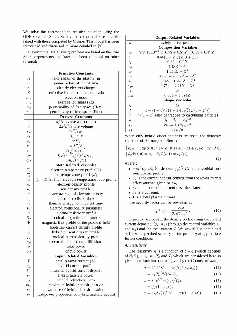
Output Related Variablesq safety factor profile

Composition VariablescL 3.3735 10−33Z(0.73 + 0.27Z)/(0.53 + 0.47Z)cr 0.56(3− Z)/(Z(3 + Z))cξ 0.58 + 0.2Zch 1.18Z−0.24

d0 1.414Z + Z2

d1 0.754 + 2.657Z + 2Z2

d2 0.348 + 1.243Z + Z2

a10 0.754 + 2.21Z + Z2

a11 d2

a20 0.884 + 2.074ZShape Variables

ζ εx

f 1− (1− ζ)2/(1 + 1.46

√ζ)

√(1− ζ2)

)r f/(1− f) ratio of trapped to circulating particlesd d0 + d1r + d2r

2

a1 r(a10 + ra11)/da2 a20r/d

When only hybrid effect antennas are used, the dynamicequation of the magnetic flux is :

∂tΨ = Rη(∂xΨ, t)(jb(∂xΨ, t) + jh(t) + cj

1x∂x(x∂xΨ)

),

∂xΨ(t, 0) = 0, ∂xΨ(t, 1) = cII(t),(9)

where :• −cj

1x∂x(x∂xΨ), denotedjϕ(Ψ, t), is the toroidal cur-

rent plasma profile,• jh is the current deposit coming from the lower hybrid

effect antenna given below,• jb is the bootstrap current described later,• cj is a constant,• I is a total plasma current.The security factor can be rewritten as :

q(t, x) =−cqx

∂xΨ(t, x). (10)

Typically, we control the density profile using the hybridcurrent depositjh(ph, nh) (through the control variablesph

andnh) and the total currentI. We would like obtain andstabilize a specified security factor profileq at appropriatefusion conditions.

A. Resistivity

The resistivityη is a function of : –q (which dependsof ∂xΨ), – ne, ni, Te andTi which are considered here asgiven time functions (in fact given by the Cronos software) :

Λ = 31.3181 + log(Te/(e

√ne)

), (11)

τe = cT T 3/2e /(Λne), (12)

ν = cνx3/2q/(τe

√Te), (13)

w = f/(1 + cξν), (14)

η = cLΛ/(T 3/2

e (1− w)(1− crw)). (15)

B. Bootstrap Current

The bootstrap current comes from a complex mechanismwhere some particles do not follow the magnetic field butare trapped in a plasma zone. The contribution of theelectron (only considered here) to the induce current is givenby :

jb = R(a1 − a2)ne∂xTe + a1Te∂xne

∂xΨ.

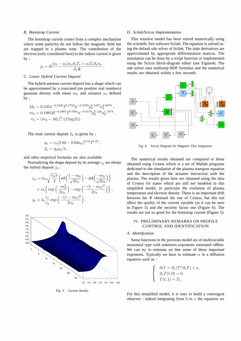
C. Lower Hybrid Current Deposit

The hybrid antenna current deposit has a shape which canbe approximated by a truncated (on positive real numbers)gaussian density with meanmh and variancevh definedby :

Mh = 0.5354−0.2446I0.5723n−0.0789p0.1337h n0.3879

h ,

mh = 0.1985B−0.3905I0.7061n−0.0178p0.126h n1.1974

h ,

vh = (mh −Mh)2/(2 log(2)) .

The total current depositIh is given by :

ηh = ch(2.03− 0.63nh)0.55I0.43 ,

Ih = ηhph/n ,

and other empirical formulas are also available.Normalizing the shape deposit by its averagecg we obtain

the hybrid depositjh :

cg = mh

√vhπ

2

erf

(1−mh√2vh

)− erf

(−mh√2vh

)+ vh

exp

(−m2h

2vh

)− exp

(−(1−mh)2

2vh

),

jh = Ihcv

cgexp

(−(x−mh)2

2vh

).

Fig. 3. Current density.

D. Scilab/Scicos Implementation

This resistive model has been solved numerically usingthe scientific free software Scilab. The equation is solved us-ing the default ode solver of Scilab. The state derivatives areapproximated by appropriate differentiation matices. Thesimulation can be done by a script function or implementedusing the Scicos block-diagram editor (see Figure4). Theode solver uses multistep BDF formulas and the numericalresults are obtained within a few seconds.

todisP

epocM liforPHLJ

orC_eT

orC_en

orC_iT orC_in

j

orc_j

q

orc_q

j

q

n

n

q

j

j

T

SS

.Ψ

T

e

e

h

ii

copecope

c

c

ccorC_iTIp

c

c

Fig. 4. Scicos Diagram for Magnetic Flux Integration.

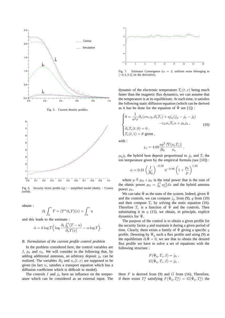
The numerical results obtained are compared to thoseobtained using Cronos which is a set of Matlab programsdedicated to the simulation of the plasma transport equationand the description of the actuator interaction with theplasma. The results given here are obtained using the dataof Cronos for states which are still not modeled in thissimplified model, in particular the evolution of plasmatemperature and electron density. There is an important driftbetween theΨ obtained the one of Cronos, but this notaffect the quality of the current variable (as it can be seenin Figure 5) and the security factor one (Figure 6). Theresults are not so good for the bootstrap current (Figure 5).

IV. PRELIMINARY REMARKS ON PROFILECONTROL AND IDENTIFICATION

A. Identification

Some functions in the previous model are of multivariablemonomial type with unknown exponents estimated offline.We can try to estimate on line some of these importantexponents. Typically we have to estimateα in a diffusionequation such as :

∂tT = ∂x(Tα∂xT ) + u,

∂xT (t, 0) = 0,

T (t, 1) = T1.

For this simplified model, it is easy to build a convergentobserver : indeed integrating from0 to x the equation we

0.0 0.2 0.4 0.6 0.8 1.00.0

0.5

1.0

1.5

2.0

2.5

j

Cronos

Simulation

j

j

b

h

φ

Fig. 5. Current density profiles.

0.0 0.1 0.2 0.3 0.4 0.5 0.6 0.7 0.8 0.9 1.00

1

2

3

4

5

6

7

8

Fig. 6. Security factor profile (q) : – simplified model (dash), – Cronos(solid).

obtain :

∂t

∫ x

0

T = (Tα∂xT )(x) +∫ x

0

u

and this leads to the estimate :

α = k log T(

log∂t

∫ x

0(T − u)

∂xT (x)− α log T

).

B. Formulation of the current profile control problem

In the problem considered here, the control variables areI, ph and nh. We will consider in the following that, byadding additional antennas, an arbitrary depositjh can berealized. The variablesB0 andne(t, x) are supposed to begiven (in factne satisfies a transport equation which has adiffusion coefficient which is difficult to model).

The controlsI and jh have an influence on the temper-ature which can be considered as an external input. The

0 3 6 9 12 15 18 21 24−1

0

1

2

3

+

Fig. 7. Estimator Convergence (α = 2, uniform noise belonging to[−0.4, 0.4] on the derivative).

dynamic of the electronic temperatureTe(t, x) being muchfaster than the magnetic flux dynamics, we can assume thatthe temperature is at its equilibrium. At each time, it satisfiesthe following static diffusion equation (which can be derivedas it has be done for the equation ofΨ see [1]) :

0 =1

a2x∂x(xneχe∂xTe) + ηjϕ(jϕ − jh − jb)

−cDneTeα + ρhjh ,

∂xTe(t, 0) = 0 ,

Te(t, 1) = θ given ,

(16)

with :

χe = 4.68aq2

B0

|∇(neTe)|ne

,

ρhjh the hybrid heat deposit proportional tojh andTi theion temperature given by the empirical formula (see [10]) :

α = 0.31(

I

B0

)−0.38

n−0.90

(1 +

ph

p

)1.36

wherep , pΩ + ph is the total power that is the sum ofthe ohmic powerpΩ =

∫ 1

0ηj2

ϕdx and the hybrid antennapowerph.

We can takeΨ as the state of the system. Indeed, givenΨand the controls, we can computejϕ from (9), q from (10)and then computeTe by solving the static equation (16).ThereforeTe is a function of Ψ and the controls. Thensubstituting it inη (15), we obtain, in principle, explicitdynamics forΨ.

The purpose of the control is to obtain a given profile forthe security factorq and maintain it during a given period oftime. Clearly, there exists a family ofΨ giving a specificqprofile. Denoting byΨq such a flux profile and using (9) atthe equilibrium∂tΨ = 0, we see that to obtain the desiredflux profile we have to solve a set of equations with thefollowing structure :

F (Ψq, Te, I) = jh ,

G(Ψq, Te, I) = jh .

Here F is derived from (9) andG from (16). Therefore,if there existsT q

e satisfyingF (Ψq, Tqe ) = G(Ψq, T

qe ) the

above compatibility conditions are satisfied and the corre-sponding controljh gives the desired equilibrium aroundwhich the system should be stabilized.

The variableΨ is not observed but we are able to observeTe. From Te and the control, using (16) (where we seeΨas unknown) and the boundary conditions of (9), we cancomputeΨ.

Summarizing, supposing that we have enough antennato be able to approximate any deposit profile, we have tocontrol a nonlinear system where we can consider that : –we observe the state, – the system is controllable

V. CONCLUSION

The nonlinear model given here aims at providing reliablesimulation results. As such it can be used to validate controllaws. Based on the profile obtained it seems that we canobtain simpler nonlinear model to design the control law.

REFERENCES

[1] J. Blum, Numerical Simulation and Optimal Control in PlasmaPhysics, Gauthier-Villars, 1989.

[2] F. Imbeaux, V. Basiuk, J.-F. Artaud, M. Schneider,Cronos User’sGuide Technical Note, PHY/NTT-2006.002, CEA/DSM/DRFC,2006.

[3] IEEE Control System Magazine,Special Issue on Fusion, October2005.

[4] IEEE Control System Magazine,Special Issue on Fusion, April 2006.[5] L. Laborde,Controle des profils de courant et de pression en temps

reel dans les plasmas de tokamaks, Phd Thesis Dec. 2005, ProvenceUniversity.

[6] M. L. Walker, D. A. Humphreys, D. Mazon, D. Moreau, M. Ok-abayashi, T. H. Osborne, E. Schuster,Emerging Applications inTokamak Plasma ControlIEEE Control Systems Magazine, April2006.

[7] D. Moreau and all,New Dynamic-Model Approach for SimultaneousControl of Distributed and Kinetic Parameters in the ITER-like JETPlasmas, 21 IAEA Fusion Energy Conf. Chengdu (China) October2006.

[8] J. Wesson,Tokamaks, Oxford Science Publications, 2004.[9] E. Witrant, E. Joffrin, S. Bremond, G. Giruzzi, D. Mazon, O. Barana,

P. Moreau,A Control Oriented Model of the Flux Diffusion inTokamak Plasma, personal communication.

[10] E. Witrant, Parameter Dependant Identification of Nonlinear Dis-tributed Systems: Application to Tokamak Plasmas, submitted toIEEE Transactions on Control Systems Technologies, 2007.