Experimental study of shear in reinforced concrete one way slabs subjected to concentrated loads

Abstract—Designing two-way slabs under transverse
concentrated loads is one of the challenges in designing such structures. No certain method can be found in the design codes or references for designing two-way slabs subjected to concentrated loads. However, plastic method can be the best method for designing such cases of two-way slabs. This method requires various formulas for different conditions of RC slab and so, is practically not simple and not usable in designing offices. In this paper, plastic method is used for different conditions of RC slabs and also various dimensions, in order to derive the essential formulas followed by calculating the positive and negative moment coefficients for concentrated loading located in different points of a two-way slab. The efficiency of this method is shown by a numeric example at the end of the paper.
Index Terms—Concentrated loading, plastic method, RC two-way slab, yield lines.
I. INTRODUCTION Accurate analysis of two-way slabs having different
continuity conditions at their edges is very difficult and for practical purposes is almost impossible. Thus, there are several simplified methods for determining the moments, shear forces and support reactions [1]-[2]. The methods used for designing RC members are mostly based on elastic analysis of the structure subjected to the ultimate loads though, the actual behavior of an indeterministic structure is that when one or more member reach its bending resistance, the elastic diagrams of this part will change to some extend and so, the elastic analysis results cannot be used anymore. In such case if the structure has sufficient ductility, each time that the section reaches its bending resistance, the bending moments will redistribute until some plastic hinges or plastic lines form and, the structure becomes unstable. In such circumstances, the structure cannot resist any more load and collapses (see Fig. 1). Such type of analysis in which the bending moment diagrams at the failure point are used as a basis for the design, is called plastic analysis [3]. Although there are some other methods for analyzing and designing RC slabs subjected to concentrated load such as finite elements, finite difference methods, and also using the plate’s theory method, but still the best and most practical available method is the plastic method.
Manuscript received April 15, 2013; revised July 2, 2013. Morteza Fadaee and Atefeh Iranmanesh are with Civil Eng. Dept., Shahid
Bahonar Univ. of Kerman, Kerman, Iran (e-mail: [email protected]; [email protected]).
M. Javad Fadaee is with Civil Eng. Dept., Shahid Bahonar Univ. of Kerman, Kerman, Iran (e-mail: [email protected]).
Fig. 1. Failure mechanism in a slab. In plastic method which is also known as the yield lines
method, it is assumed that the resistance of the slab is determined by bending only, and the other factors such as shear or displacement should be considered separately.
It must be noted that in the yield lines method the behavior of the slab can be considered better. Many of slab systems which cannot be analyzed with other methods such as equivalent frame method, direct method and moment coefficients method because of the slab specific shape or loading type, can be designed by plastic method. In fact, by the plastic method it is possible to design any type of slabs with any shape subjected to any type of loadings.
Yield lines method is used for slabs which are reinforced at any direction, which means that the section area of the reinforcement is assumed constant per unit length, although the value of the reinforcement can vary in the upper face or the bottom face of the slab. It is also possible to use the yield line analysis for slabs with non-uniform reinforcement distribution, though it may be more difficult [3].
Fig. 2. Triangular failure schema for concentrated load.
II. YIELD LINE PATTERN FOR CONCENTRATED LOAD In the case of existence of a concentrated load, the schema
of failure may include the yield lines around of the load. The failure schema that contains the curved yield lines for the negative moment and the radial yield lines for the positive
A Simplified Method for Designing RC Slabs under Concentrated Loading
Morteza Fadaee, Atefeh Iranmanesh, and Mohammad J. Fadaee
IACSIT International Journal of Engineering and Technology, Vol. 5, No. 6, December 2013
675DOI: 10.7763/IJET.2013.V5.640
moment would be more critical than the failure schema with triangular segments among the yield lines [1], However, in this paper the triangular failure schema is used for the concentrated load and the calculations are based on this type of schema, (see Fig. 2).
III. EQUATIONS FOR MOMENT COEFFICIENTS CALCULATION In this section, the relations of the plastic method for the
rectangular slabs having simple or fixed supported edges are obtained. For this purpose, the internal work is considered equal to the external work based upon the following equation,
∑ ∑ =+ δθθ Plmlm xyuyyxux
(1)
where uxuy mm , are moments per unit length about the x and
y axes, respectively, xy θθ , are the yield lines’ rotation angles
about the x and y axes, respectively, xy ll , are the yield lines’
lengths along the x and y axes, respectively, P is the concentrated load and δ is the displacement under the application point of the concentrated load. In this work, the slab is assumed to be isotropic, therefore, uuyux mmm == .
For a rectangular slab with simple supported edges, the following relation can be obtained from (1),
)1()1( nba
mab
nba
mab
Pmu
−+
−++
=
(2)
)1()1(111
nr
mrnr
mr
f
−+
−++
=
(3)
where, bar = . For rectangular slabs with fixed supported
edges, (1) results in the following equation,
)1()1( nba
mab
nba
mab
Pmm uu
−+
−++
=+ −+
(4)
))1()1(
11(5.2
1
nr
mrnr
mr
f
−+
−++
=
(5)
By similar calculations the relations needed for other conditions of the slab edges, can be determined.
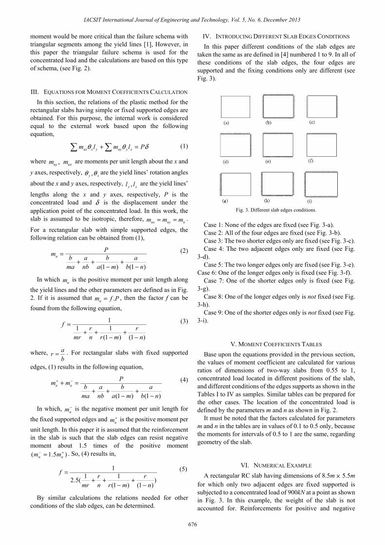
IV. INTRODUCING DIFFERENT SLAB EDGES CONDITIONS In this paper different conditions of the slab edges are
taken the same as are defined in [4] numbered 1 to 9. In all of these conditions of the slab edges, the four edges are supported and the fixing conditions only are different (see Fig. 3).
Fig. 3. Different slab edges conditions.
Case 1: None of the edges are fixed (see Fig. 3-a). Case 2: All of the four edges are fixed (see Fig. 3-b). Case 3: The two shorter edges only are fixed (see Fig. 3-c). Case 4: The two adjacent edges only are fixed (see Fig.
3-d). Case 5: The two longer edges only are fixed (see Fig. 3-e).
Case 6: One of the longer edges only is fixed (see Fig. 3-f). Case 7: One of the shorter edges only is fixed (see Fig.
3-g). Case 8: One of the longer edges only is not fixed (see Fig.
3-h). Case 9: One of the shorter edges only is not fixed (see Fig.
3-i).
V. MOMENT COEFFICIENTS TABLES Base upon the equations provided in the previous section,
the values of moment coefficient are calculated for various ratios of dimensions of two-way slabs from 0.55 to 1, concentrated load located in different positions of the slab, and different conditions of the edges supports as shown in the Tables I to IV as samples. Similar tables can be prepared for the other cases. The location of the concentrated load is defined by the parameters m and n as shown in Fig. 2.
It must be noted that the factors calculated for parameters m and n in the tables are in values of 0.1 to 0.5 only, because the moments for intervals of 0.5 to 1 are the same, regarding geometry of the slab.
VI. NUMERICAL EXAMPLE A rectangular RC slab having dimensions of 8.5m × 5.5m
for which only two adjacent edges are fixed supported is subjected to a concentrated load of 900kN at a point as shown in Fig. 3. In this example, the weight of the slab is not accounted for. Reinforcements for positive and negative
IACSIT International Journal of Engineering and Technology, Vol. 5, No. 6, December 2013
676
In which um is the positive moment per unit length along the yield lines and the other parameters are defined as in Fig. 2. If it is assumed that Pfmu .= , then the factor f can be found from the following equation,
In which, −um is the negative moment per unit length for
the fixed supported edges and +um is the positive moment per
unit length. In this paper it is assumed that the reinforcement in the slab is such that the slab edges can resist negative moment about 1.5 times of the positive moment
)5.1( +− = uu mm . So, (4) results in,

moments at the edges are calculated as follows. Parameters needed for calculating the factor f can be found
as follows,
TABLE I: CONCENTRATED LOAD COEFFICIENTS FOR SLAB CASE 1
r 0.55 0.6 0.65 0.7 0.75 0.8 0.85 0.9 0.95 1 m n f
0.1
0.1 0.038 0.0397 0.0411 0.0423 0.0432 0.0439 0.0444 0.0448 0.0449 0.045 0.2 0.0423 0.0449 0.0473 0.0494 0.0513 0.0529 0.0544 0.0556 0.0567 0.05760.3 0.0438 0.0468 0.0495 0.0521 0.0544 0.0565 0.0584 0.0601 0.0617 0.063 0.4 0.0445 0.0476 0.0505 0.0532 0.0557 0.0581 0.0602 0.0621 0.0639 0.06550.5 0.0446 0.0478 0.0508 0.0536 0.0561 0.0585 0.0607 0.0627 0.0645 0.0662
0.2
0.1 0.0572 0.0585 0.0594 0.0599 0.06 0.0599 0.0595 0.059 0.0584 0.05760.2 0.0676 0.0706 0.0731 0.0752 0.0768 0.078 0.079 0.0796 0.0799 0.08 0.3 0.0715 0.0753 0.0787 0.0816 0.084 0.086 0.0877 0.089 0.0901 0.09080.4 0.0732 0.0774 0.0811 0.0844 0.0873 0.0897 0.0918 0.0935 0.0949 0.096 0.5 0.0737 0.078 0.0819 0.0853 0.0882 0.0908 0.093 0.0948 0.0963 0.0976
0.3
0.1 0.0677 0.0685 0.0687 0.0686 0.0681 0.0674 0.0665 0.0654 0.0642 0.063 0.2 0.0827 0.0856 0.0878 0.0895 0.0906 0.0913 0.0916 0.0916 0.0913 0.09080.3 0.0887 0.0926 0.096 0.0987 0.1008 0.1024 0.1036 0.1044 0.1049 0.105 0.4 0.0913 0.0958 0.0997 0.1029 0.1055 0.1077 0.1094 0.1106 0.1115 0.112 0.5 0.0921 0.0967 0.1007 0.1041 0.107 0.1093 0.1111 0.1125 0.1135 0.1141
0.4
0.1 0.0731 0.0735 0.0734 0.0728 0.072 0.0709 0.0697 0.0684 0.0669 0.06550.2 0.0908 0.0935 0.0955 0.0968 0.0976 0.098 0.0979 0.0975 0.0969 0.096 0.3 0.0981 0.102 0.1052 0.1077 0.1096 0.1109 0.1117 0.1122 0.1122 0.112 0.4 0.1013 0.1059 0.1097 0.1128 0.1152 0.1171 0.1184 0.1193 0.1198 0.12 0.5 0.1023 0.107 0.111 0.1143 0.1169 0.1189 0.1205 0.1215 0.1222 0.1224
0.5
0.1 0.0747 0.075 0.0748 0.0741 0.0732 0.072 0.0707 0.0692 0.0677 0.06620.2 0.0934 0.096 0.0979 0.0991 0.0998 0.1 0.0998 0.0993 0.0985 0.09760.3 0.1011 0.105 0.1081 0.1105 0.1123 0.1135 0.1142 0.1145 0.1145 0.11410.4 0.1046 0.1091 0.1128 0.1159 0.1182 0.12 0.1212 0.122 0.1224 0.12240.5 0.1056 0.1103 0.1142 0.1174 0.12 0.122 0.1234 0.1243 0.1248 0.125
TABLE II: CONCENTRATED LOAD COEFFICIENTS FOR SLAB CASE 2
r 0.55 0.6 0.65 0.7 0.75 0.8 0.85 0.9 0.95 1 m n f
0.1
0.1 0.0152 0.0159 0.0164 0.0169 0.0173 0.0176 0.0178 0.0179 0.018 0.018 0.2 0.0169 0.018 0.0189 0.0198 0.0205 0.0212 0.0218 0.0223 0.0227 0.023 0.3 0.0175 0.0187 0.0198 0.0208 0.0218 0.0226 0.0234 0.0241 0.0247 0.02520.4 0.0178 0.019 0.0202 0.0213 0.0223 0.0232 0.0241 0.0249 0.0256 0.02620.5 0.0179 0.0191 0.0203 0.0214 0.0225 0.0234 0.0243 0.0251 0.0258 0.0265
0.2
0.1 0.0229 0.0234 0.0238 0.0239 0.024 0.024 0.0238 0.0236 0.0233 0.023 0.2 0.027 0.0282 0.0292 0.0301 0.0307 0.0312 0.0316 0.0318 0.032 0.032 0.3 0.0286 0.0301 0.0315 0.0326 0.0336 0.0344 0.0351 0.0356 0.036 0.03630.4 0.0293 0.031 0.0325 0.0338 0.0349 0.0359 0.0367 0.0374 0.038 0.03840.5 0.0295 0.0312 0.0327 0.0341 0.0353 0.0363 0.0372 0.0379 0.0385 0.039
0.3
0.1 0.0271 0.0274 0.0275 0.0274 0.0272 0.027 0.0266 0.0262 0.0257 0.02520.2 0.0331 0.0342 0.0351 0.0358 0.0362 0.0365 0.0366 0.0366 0.0365 0.03630.3 0.0355 0.0371 0.0384 0.0395 0.0403 0.041 0.0415 0.0418 0.0419 0.042 0.4 0.0365 0.0383 0.0399 0.0412 0.0422 0.0431 0.0437 0.0442 0.0446 0.04480.5 0.0368 0.0387 0.0403 0.0417 0.0428 0.0437 0.0444 0.045 0.0454 0.0457
0.4
0.1 0.0292 0.0294 0.0293 0.0291 0.0288 0.0284 0.0279 0.0273 0.0268 0.02620.2 0.0363 0.0374 0.0382 0.0387 0.0391 0.0392 0.0392 0.039 0.0387 0.03840.3 0.0392 0.0408 0.0421 0.0431 0.0438 0.0444 0.0447 0.0449 0.0449 0.04480.4 0.0405 0.0424 0.0439 0.0451 0.0461 0.0468 0.0474 0.0477 0.0479 0.048 0.5 0.0409 0.0428 0.0444 0.0457 0.0468 0.0476 0.0482 0.0486 0.0489 0.049
0.5
0.1 0.0299 0.03 0.0299 0.0296 0.0293 0.0288 0.0283 0.0277 0.0271 0.02650.2 0.0373 0.0384 0.0392 0.0396 0.0399 0.04 0.0399 0.0397 0.0394 0.039 0.3 0.0404 0.042 0.0432 0.0442 0.0449 0.0454 0.0457 0.0458 0.0458 0.04570.4 0.0418 0.0436 0.0451 0.0463 0.0473 0.048 0.0485 0.0488 0.049 0.049 0.5 0.0422 0.0441 0.0457 0.047 0.048 0.0488 0.0493 0.0497 0.0499 0.05
Fig. 4. Numerical example.
65.05.85.5,4.0
84.3,3.0
5.565.1 ≈===== rnm
So, the factor f from the Table IV is determined as 0.0574, thus,
.0.0574 0.0574 900 51.66u
kN mf mm
+= ⇒ = × =
As the negative moment is assumed 1.5 times of the
positive moment, therefore, the negative moment per unit length is calculated as follows,
IACSIT International Journal of Engineering and Technology, Vol. 5, No. 6, December 2013
677

TABLE III: CONCENTRATED LOAD COEFFICIENTS FOR SLAB CASE 3 r 0.55 0.6 0.65 0.7 0.75 0.8 0.85 0.9 0.95 1
m n f
0.1
0.1 0.0282 0.0284 0.0284 0.0283 0.0281 0.0277 0.0273 0.0268 0.0263 0.02570.2 0.0347 0.0359 0.0367 0.0373 0.0377 0.0379 0.0379 0.0379 0.0377 0.03740.3 0.0374 0.039 0.0403 0.0413 0.0421 0.0427 0.0431 0.0434 0.0435 0.04340.4 0.0386 0.0404 0.0419 0.0432 0.0442 0.045 0.0456 0.046 0.0463 0.04650.5 0.0389 0.0408 0.0424 0.0437 0.0448 0.0457 0.0464 0.0468 0.0472 0.0474
0.2
0.1 0.0375 0.0369 0.0361 0.0352 0.0343 0.0333 0.0323 0.0313 0.0303 0.02940.2 0.0501 0.0505 0.0506 0.0503 0.0499 0.0492 0.0485 0.0476 0.0467 0.04570.3 0.0558 0.0569 0.0576 0.0579 0.0579 0.0577 0.0572 0.0566 0.0559 0.05510.4 0.0585 0.06 0.061 0.0617 0.0619 0.0619 0.0617 0.0613 0.0607 0.06 0.5 0.0593 0.0609 0.0621 0.0628 0.0632 0.0632 0.0631 0.0627 0.0622 0.0615
0.3
0.1 0.0418 0.0406 0.0394 0.0381 0.0368 0.0355 0.0342 0.033 0.0318 0.03070.2 0.058 0.0578 0.0572 0.0564 0.0553 0.0542 0.053 0.0517 0.0504 0.04910.3 0.0658 0.0663 0.0664 0.0661 0.0655 0.0646 0.0636 0.0625 0.0613 0.06 0.4 0.0695 0.0705 0.0709 0.071 0.0706 0.07 0.0692 0.0682 0.0671 0.06590.5 0.0706 0.0718 0.0723 0.0724 0.0722 0.0717 0.0709 0.07 0.0689 0.0677
0.4
0.1 0.0438 0.0424 0.0409 0.0394 0.0379 0.0365 0.0351 0.0338 0.0325 0.03130.2 0.0618 0.0613 0.0604 0.0592 0.0579 0.0565 0.055 0.0535 0.052 0.05050.3 0.0708 0.071 0.0707 0.07 0.069 0.0679 0.0666 0.0652 0.0637 0.06220.4 0.0752 0.0758 0.0759 0.0755 0.0748 0.0738 0.0727 0.0714 0.07 0.06860.5 0.0765 0.0773 0.0775 0.0772 0.0766 0.0757 0.0746 0.0734 0.072 0.0706
0.5
0.1 0.0443 0.0429 0.0413 0.0397 0.0382 0.0367 0.0353 0.034 0.0327 0.03150.2 0.063 0.0623 0.0613 0.0601 0.0586 0.0571 0.0556 0.054 0.0525 0.051 0.3 0.0724 0.0724 0.072 0.0712 0.0701 0.0689 0.0675 0.066 0.0644 0.06290.4 0.0769 0.0774 0.0774 0.0769 0.0761 0.075 0.0737 0.0724 0.0709 0.06940.5 0.0783 0.0789 0.079 0.0787 0.0779 0.0769 0.0757 0.0744 0.0729 0.0714
TABLE IV: CONCENTRATED LOAD COEFFICIENTS FOR SLAB CASE 4
r 0.55 0.6 0.65 0.7 0.75 0.8 0.85 0.9 0.95 1 m n f
0.1
0.1 0.0183 0.0195 0.0206 0.0216 0.0225 0.0225 0.024 0.0247 0.0252 0.02570.2 0.0261 0.0279 0.0295 0.031 0.0324 0.0324 0.0347 0.0357 0.0366 0.03740.3 0.0302 0.0323 0.0342 0.0359 0.0375 0.0375 0.0403 0.0415 0.0425 0.04340.4 0.0326 0.0348 0.0368 0.0386 0.0403 0.0403 0.0432 0.0444 0.0455 0.04650.5 0.0339 0.0361 0.0381 0.0399 0.0416 0.0416 0.0443 0.0455 0.0465 0.0474
0.2
0.1 0.0219 0.0232 0.0244 0.0254 0.0264 0.0264 0.0279 0.0285 0.029 0.02940.2 0.0339 0.036 0.0378 0.0395 0.0409 0.0409 0.0433 0.0443 0.0451 0.04570.3 0.0412 0.0437 0.0459 0.0478 0.0496 0.0496 0.0523 0.0534 0.0543 0.05510.4 0.0458 0.0484 0.0507 0.0528 0.0545 0.0545 0.0574 0.0584 0.0593 0.06 0.5 0.0484 0.051 0.0532 0.0552 0.0569 0.0569 0.0594 0.0603 0.061 0.0615
0.3
0.1 0.0233 0.0246 0.0258 0.0269 0.0278 0.0278 0.0293 0.0299 0.0304 0.03070.2 0.0374 0.0395 0.0414 0.0431 0.0446 0.0446 0.0469 0.0478 0.0485 0.04910.3 0.0464 0.049 0.0513 0.0533 0.055 0.055 0.0576 0.0586 0.0594 0.06 0.4 0.0522 0.055 0.0574 0.0594 0.0612 0.0612 0.0638 0.0647 0.0654 0.06590.5 0.0557 0.0584 0.0606 0.0625 0.0641 0.0641 0.0663 0.067 0.0675 0.0677
0.4
0.1 0.0239 0.0252 0.0265 0.0275 0.0285 0.0285 0.0299 0.0305 0.0309 0.03130.2 0.0389 0.0411 0.043 0.0447 0.0462 0.0462 0.0485 0.0493 0.05 0.05050.3 0.0489 0.0515 0.0538 0.0558 0.0575 0.0575 0.06 0.061 0.0617 0.06220.4 0.0554 0.0582 0.0606 0.0626 0.0643 0.0643 0.0668 0.0676 0.0682 0.06860.5 0.0592 0.0619 0.0642 0.0661 0.0675 0.0675 0.0695 0.0701 0.0705 0.0706
0.5
0.1 0.0241 0.0254 0.0266 0.0277 0.0286 0.0286 0.0301 0.0307 0.0311 0.03150.2 0.0394 0.0416 0.0435 0.0452 0.0467 0.0467 0.0489 0.0498 0.0504 0.051 0.3 0.0496 0.0522 0.0545 0.0565 0.0582 0.0582 0.0608 0.0617 0.0624 0.06290.4 0.0563 0.0591 0.0615 0.0635 0.0652 0.0652 0.0676 0.0684 0.069 0.06940.5 0.0603 0.063 0.0653 0.0671 0.0686 0.0686 0.0705 0.071 0.0713 0.0714
1.5 1.5 51.66 77.49 . /u um m kN m m− += = × =
Now the reinforcement of positive and negative moments
can be determined based upon a design Code. In this example CCI (Concrete Code of Iran) [5] is used. The thicknesses of the slab h, and the effective depth d are taken as 18cm and 15cm, respectively. The concrete’s compressive strength fc and steel’s yield stress fy are 21MPa and 400MPa, respectively. Thus,
mmmA
mmkNm su
2
82.1153,66.51 =⇒= ++
mmmA
mmkNm su
2
38.1902.49.77 =⇒= −−
in longitudinal direction,
⎪⎩
⎪⎨⎧
⇒=
⇒=−
+
mmUSEmmA
mmUSEmmA
s
s
2
φφ
in latitudinal direction,
⎪⎩
⎪⎨⎧
⇒=
⇒=−
+
mmUSEmmA
mmUSEmmA
s
s
2
φφ
IACSIT International Journal of Engineering and Technology, Vol. 5, No. 6, December 2013
678

The plan of the slab’s reinforcement is shown in Fig. 5:
Fig. 5. Reinforcement of the example.
VII. CONCLUSION As no practical method for designing two-way RC slabs
subjected to concentrated load can be found in RC books, publications and codes, in this research using the plastic method (yield lines method) which is an appropriate method for designing the slabs subjected to concentrated load, moment coefficients for different conditions of slab edges supports and various slab dimensions and different points of application of the loadings have been provided that can be used for designing RC slabs practically at the engineering offices.
REFERENCES [1] A. M. Kaynia, Calculation and Designing of Concrete Structures, 6th
ed. Isfahan: Isfahan’s Jahad Daneshgahi, 1996, ch. 11, pp. 533-564. [2] F. Pourshahsavari and M. J. Fadaee, “Comparing the Moment
Coefficients Method and the Plastic Method in RC Slabs Designing,” in Proc. of 5th National Congress of Civil Engineering, Mashhad, 2010, pp.
[3] A. R. Rahaii, Reinforced Concrete Structures (Design and Calculation), 1st ed. Tehran: Amir-Kabir University of Technology, 1999, ch. 15, pp. 544-552.
[4] G. Winter, L. C. Urquhart, C. E. O. O’Rourke, and A. H. Nilson, Design of Concrete Structures, 7th ed. New York, McGraw-Hill, 1964, ch. 4, pp 200-203.
[5] Concrete Code of Iran, Iranian Standard-2000.
Morteza Fadaee was born in December 7, 1989 in Kerman, Iran. Morteza has spent some of his school classes in Waterloo, Canada. After coming back to Iran, he spent his secondary and high school grades at Kerman’s Allameh-Helli (NODET) high school. Now he is studying at Civil Engineering Department of Shahid Bahonar University of Kerman. He is also working for a consulting engineers co. in
Kerman for 2 years and have been worked for some other companies in his past. He is teacher assistant in some courses in his university now, and was TA in Besat College of Kerman last year.
Atefeh Iranmanesh was born in March 9, 1990 in Kerman, Iran. She spent her secondary and high school grades at Kerman’s Farzanegan (NODET) high school. Now she is studying at Civil Engineering Department of Shahid Bahonar University of Kerman.
She is working for a consulting engineers co. in Kerman for one year.
Mohammad Javad Fadaee was born in July 7, 1958 in Kerman, Iran. He completed his B.Sc. and M.Sc. degrees at University of Tehran, Tehran, Iran. He got his Ph.D. degree in 1996 from University of Waterloo, Ontario, Canada.
He has worked in various organizations and companies after his graduation. He is now an associate professor in his hometown university; Shahid Bahonar
University of Kerman, Kerman, Iran. He has more than 26 years’ experience of teaching and researching. He has published more than 120 papers in journals and conference proceedings in his main field, optimization and other Civil Engineering fields.
Dr. Fadaee is a member of ASCE and some other societies in his fields of study in Iran.
IACSIT International Journal of Engineering and Technology, Vol. 5, No. 6, December 2013
679