A Simple Stochastic Model for Generating Broken Cloud Optical Depth

and Top Height Fields

Sergei M. Prigarin1 and Alexander ~ a r s h a k ~

1 Novosibirsk State University and Institute of Computational Mathematics and

Mathematical Geophysics, Russian Academy of Sciences (Siberian Branch),

Novosibirsk, Russia

2 N A S ~ - Goddard Space Flight Center, Climate and Radiation Branch, Maryland, USA

Correspondence

Alexander Marshak

tel. 301-6146122

email: Alexander.Marshak@nasa.gov

Prepared for publication in

JOURNAL OF THE A TMOSPHERIC SCIENCES

Submitted: December 9,2007

A Simple Stochastic Model for Generating Broken Cloud Optical Depth

and Top Height Fields

Abstract

A simple and fast algorithm for generating two correlated stochastic two-

dimensional (2D) cloud fields is described. The algorithm is illustrated with two broken

cumulus cloud fields: cloud optical depth and cloud top height retrieved from Moderate

Resolution Imaging Spectrometer (MODIS). Only two 2D fields are required as an input.

The algorithm output is statistical realizations of these two fields with approximately the

same correlation and joint distribution functions as the original ones. The major

assumption of the algorithm is statistical isotropy of the fields. In contrast to fractals and

the Fourier filtering methods frequently used for stochastic cloud modeling, the proposed

method is based on spectral models of homogeneous random fields. For keeping the

same probability density function as the (first) original field, the method of inverse

distribution function is used. When the spatial distribution of the first field has been

generated, a realization of the correlated second field is simulated using a conditional

distribution matrix. This paper is served as a theoretical justification to the publicly

available software that has been recently released by the authors and can be freely

downloaded from http://i3rc.gsfc.nasa.gov/Public codes clouds.htm. Though 2D rather

than full 3D, stochastic realizations of two correlated cloud fields that mimic statistics of

given fields have proved to be very useful to study 3D radiative transfer features of

broken cumulus clouds for better understanding of shortwave radiation and interpretation

of the remote sensing retrievals.

1. Introduction

In order to better understand and predict shortwave radiation in realistic cloudy

atmospheres, we need to specify 3D distribution of cloud liquid water. Also, statistical

cloud retrievals that include 3D radiative transfer require a large number of 3D cloud

fields (Evans et al., 2007). Realistic cloud fields and spatial distributions of cloud liquid

water can be obtained from either dynamical or stochastic cloud models. Based on cloud

dynamics, physical (or dynamical) cloud models such as a large eddy simulation (LES) or

a cloud resolving model (e.g., Ackerman et al., 1995) are physically consistent but

require specification of a lot of atmospheric parameters and often are computationally

expensive. On the other hand, stochastic cloud models based on aircraft, satellite or

ground measurements of cloud structure are computationally inexpensive though they are

mostly 2D since currently there are no techniques to measure a full 3D cloud structure.

For the last two decades many different cloud stochastic models have been

developed. We break them into two classes. The first class of cloud models uses only a

few parameters to simulate the main aspects of the realistic cloud fields like mean,

standard deviation and correlation often assumed to be a power-law. These models are

very simple and are generally used to test hypothesis and better understand cloud-

radiation interaction. These are the fractionally-integrated cascade model (Scherzer and

Lovejoy, 1987), the bounded cascades (Cahalan, 1994; Marshak et al., 1994), the

fractional Brownian motion (Voss, 1995), the Fourier filtering of Gaussian noise (Barker

and Davies, 1992; Evans, 1993; Varnai 2000), the Poisson distribution of cloud elements

(Zuev and Titov, 1995) to name a few. These models generally produce an unbroken

(overcast) 2D x-y field of cloud optical depth or cloud liquid water path. To obtain the ' desired cloud fraction, a simple threshold can be used (e.g., Barker and Davies, 1992;

Marshak et al., 1998).

The second class of cloud stochastic models provides a statistical reconstruction

of an observed field and generates the detailed cloud structure. They are also called

statistical cloud generators (Venema et al., 2006, Schmidt et al., 2007). These cloud

models are usually 3D rather than 2D. For cumulus clouds, Evans and Wiscombe (2004)

use time-height radar data to generate 2D realizations of cloud liquid water that are

generalized to 3D fields assuming statistical homogeneity and horizontal isotropy. For

stratocumulus clouds, Di Giuseppe and Tompkins (2003) generate 3D cloud liquid water

fields combining stochastic horizontal models based on power spectrum and Fourier

filtering (at each height) with realistic vertical profiles of total water and temperature.

From radar time-height series using Fourier transform technique, Hogan and Kew (2005)

generate realistic 3D cirrus cloud with fallstreak structure changing vertically the slope of

the power spectrum. Venema et al. (2006a,b) generate a surrogate cloud field with liquid

water distribution and spatial correlation (through power spectrum) statistically similar to

the observed one. Venema et al., (2006b) also compare radiative properties of LES

clouds with its surrogate fields and Venema et al., (2006a) provide an excellent review of

different cloud generators. Finally, we mention the Scheirer and Schmidt (2005)

generator that reproduces cloud fields of liquid water and effective radius using aircraft

data. Schmidt et al. (2007) used cloud fields simulated by the last three generators as

input to a 3D radiative transfer model to compare its output with the radiative flux

measurements.

The current paper describes a simple stochastic model that belongs to the second

class of cloud stochastic models. For given 2D fields of cloud optical depth and cloud

top height, the model generates realizations of these two fields with the same correlation

function and joint distribution as the original ones. In contrast to Evans and Wiscombe

(2003), it does not generate 3D cloud liquid water fields but rather provides the x-y fields

of cloud optical and geometrical thicknesses (assuming a constant cloud based). To

simulate the required autocorrelation function, it uses spectral models of homogeneous

random fields (Prigarin, 1995, 200 1) rather than commonly used Fourier filtering (e.g.,

Evans, 1993; Di Giuseppe and Tompkins, 2003; Evans and Wiscombe, 2004; Hogan and

Kew, 2005; Venema et al., 2006b). Another distinguishable feature of this paper is that it

provides a theoretical background to the publicly available software that has been

recently developed and released by the authors. (To download, go to

http://i3rc.gsfc.nasa.gov/Public codes clouds.htm and click on PDF-based stochastic

cloud model or go directly to

htt~://ser~eim.~ri~arin.~oo~lepa~es.com/SimCloudField2.WEB.ziw). Note that at

present, the software runs only on Windows PCs.

The plan of the paper is as follows. Next section briefly discusses two stochastic

models of broken cloudiness that are based on a truncated Gaussian homogeneous field.

The (auto)correlation function of a 2D field defines its structure. Section 3 describes how

to generate a quasi-Gaussian field with a given autocorrelation function that is retrieved

from the covariance of the indicator function of the original field. Section 4 then explains

how to modify the field to reproduce the observed distribution. Finally in Section 5 we

generate the second field using joint distribution of the given fields of cloud optical depth

and cloud top height. Section 6 illustrates the theory with MODIS data while Section 7

summarizes the main steps of the proposed algorithm and discusses its applications.

Section 8 gives a brief summary of the results. At the end, the Appendix demonstrates

the relations between the covariance functions of a Gaussian random filed and its

indicators.

2. Quasi-Gaussian model of broken cloudiness

Let us assume that our cloud field has a constant cloud base at height Ho and a

variable cloud top described by

Here v(x,y) is a homogeneous Gaussian field with zero mean and unit variance, and a

normalized correlation function K(x,y) (with K(0,0)=1). The point (x,y,z) belongs to a

cloud if Ho s z I w(x,y). A value w(x,y) = Ho simply means that there is a cloud gap in

the horizontal point (x,y). The cloud top field w has two parameters: a and d. Parameter

a > 0 stretches the cloud top field vertically and parameter d defines the truncation level

(compare with Marshak et al., 1998).

Simultaneously with Eq. (la) we consider another model [Kargin and Prigarin,

19881 of cloud top,

We will call Eqs. (la) and ( lb) by model A and B, respectively. Figure 1 illustrates the

difference between the two models. We can see that for model A, positive d corresponds

to a broken cloud field while negative d rather corresponds to a more "overcast" cloud

with a few gaps. It can be easily shown that cloud fraction A, has a different value for

both models, namely:

for model A,

for model B, where

is the cumulative normal distribution function which ranges between 0 and 0.5 for

negative d and between 0.5 to 1 for the positive ones.

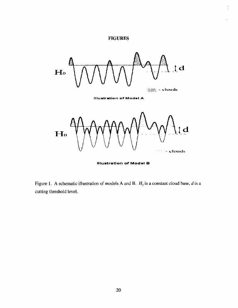
For both models we can determine the average number of clouds per unit area, m,.

Obviously m, will depend on d and autocorrelation function K. For isotropic fields, one

obtains (e.g., Sveshnikov, 1968, Eq. (45.51), pg. 441)

where i=l for model A and i=2 for model B. Here k > 0 is the second derivative of K(x,y)

with respect to x or y (which are equal for isotropic fields). Figure 2 shows the

dependence of m, on cloud fraction A, for both models and isotropic fields. We see that

number of clouds first increases with cloud fraction and then decreases. This is because

cloud fraction A, itself monotonically decreases with the truncation level d while number

of clouds m, first increases with d then decreases (see Fig. 1). Note that for model A,

number of clouds m, for A, > 0.5 ( d 4 ) is not defined. Generalization of Eq. (3) to

anisotropic fields is straightforward [Prigarin and Marshak, 20051.

To summarize, both cloud models A and B are uniquely determined by

parameters a and d and a correlation function K. To simulate a cloud field with a given

cloud fraction A,, we first solve Eq. (2) for the truncation level d. Then one needs to

generate the correlation function K(x,y) based on some additional information on

correlation in a real cloud field. Finally, parameter a is determined from a simple one-

point statistics of the cloud top field. The most difficult part of such an approach is the

choice (or generation) of the correlation function K, it will be discussed in the next

section.

3. Correlation function

The correlation function defines the geometrical structure of a cloud field, the size

and distribution of individual clouds and space between them. Perhaps the simplest

and/or the most deterministic isotropic cloud field used in the first stochastic models can

be defined by a Bessel function of the first kind, Jo (see, Gikhman and Skorokhod, 1977,

pg. 87). In this case, the correlation function

where parameter p is responsible for cloud sizes (the larger p the smaller an average

cloud is.) It is easy to see that

Thus to define p, one uses Eq. (3) that relates the average number of clouds per unit area,

m,, and second derivative k. Because p is fixed, the use of correlation function (4) is very

limited and cloud fields based on it are unrealistic (see Fig. 3 as an example).

To generalize (4), Prigarin et al. (1998) used the radial spectral density of a

Gaussian field, z(p), and representation of correlation function as an integral over all

cloud sizes p of a product between z(p) and Jo,

Here, z(p) 2 0 and iz(p)dp = 1 . Varying z(p), in general, one can get "any" correlation 0

function of a random isotropic field on the plane.

Below we briefly describe a general procedure of generating correlation function

K(x,y) based on observations leaving the details for Appendix. As an illustration, in

Section 6 we apply our algorithm to a broken cloud scene retrieved from Moderate

Resolution Imaging Spectrometer (MODIS).

Let I(x,y) be an indicator function (a binary cloud mask) that takes value 1, if

there is a cloud above point (x,y), and 0 otherwise. Based on observations, we can

estimate the mathematical expectation of I, which is a cloud fraction A,, i.e.,

and its covariance function,

KI(~,Y) = E[I(x,y) Z(0,0)1 - (8)

It is known (Ogorodnikov and Prigarin, 1996, pg. 65) that the covariance function K,(x,y)

of the indicator field Z(x,y) and correlation function K(x,y) of a Gaussian field v(x,y) are

nontrivially related (see, Appendix). This relationship allows us to retrieve correlation

function K(x,y) from the measured covariance function K,(x,y). The main steps of the

retrieval are described in Appendix. Note that the truncation level d is uniquely defined

from Eqs. (2) and (7).

4. Geometrical thickness with a given density

Equations (la) and (lb) alone do not allow us to control the distribution of cloud

geometrical thickness, w(x,y)-H,. Determined by Eqs. (la) and (1 b), this distribution is a

scaled up (a > 1) or down (a < 1) truncated (by a parameter d) Gaussian distribution; its

density is defined by

1 where q(x) = -exp(-x2 1 2) is a standard Gaussian density. However, the observed

2 n

distribution of cloud thickness does not necessarily satisfy Eq. (9). In general, one has to

modify Eqs. (la) and (lb) in order to reproduce the observed distribution. We describe

below a modification of a Gaussian model that allows reproduction of any given

distribution. This modification is based on the method of inverse distribution function

widely used in statistical modeling (e.g., Ogorodnikov and Prigarin, 1996, pg. 65-71).

Let g(h) (h > 0) be a density of the observed distribution of cloud thickness. We

denote its distribution function by

It is easy to see that if

is the distribution function with density fl(h) defined in Eq. (9) with a = 1 and 6 is a

random variable distributed with the density f, thenG-'~(e) will have a density of the

observed distribution of cloud geometrical thickness. Indeed, if F is the distribution

function of 6 then F(5) is uniformly distributed on the interval (0,l) (see, for example,

Gentle, 2003, p. 42) and thus G"F(6) will have density g.

This leads us to the following modification of Eqs. (la) and (lb):

for model A, and

for model B.

In contrast to (la) and (lb), distributions of cloud thickness w(x,y)-Ho defined by

either (12a) or (12b) match the observed probability distribution G(h). In addition, we

recall that v(x,y) is a homogeneous Gaussian field with zero mean and unit variance; its

correlation function K(x,y) is retrieved from the covariance function K,(x,y) of the

observed cloud mask field I(x,y). For both models, parameter d is uniquely determined

from the average value of I(x,y), i.e. cloud fraction A, (see (7)).

5. Joint distribution of optical and geometrical thicknesses

We assume here that we have two random variables: cloud optical depth z(x,y)

and cloud geometrical thickness h(x,y). Then a pair (z,h) will be a two-dimensional

variable and P(zl< z < z,, hl< h < h,) will be the probability that the values of z and h fall

in the intervals (z,,z2) and (h,,h,), respectively.

Practically (see next section), when two matrixes z and h are given from

observations, we first subdivide all their values into M and N bins, respectively. Then we

calculate a conditional distribution matrix,

P(m,n) = P(z is in m's bin I provided h is in n's bin), m=1, ..., M; n=l, ..., N. (13)

Now, if we assume that we have a realization of one variable, say h, then using the

conditional distribution matrix P we can simulate a distribution of a second variable, 7.

This is a straightforward procedure similar to a simulation of random number with a

given distribution. As a result for each point (x,y) we will get both z(x,y) and h(x,y).

Note that the order of simulation (first z and then h or first h and then z) is irrelevant for

the reproduction of the two-dimensional distribution.

Note that realizations of the second component generated using a conditional

distribution matrix (13) are usually more stochastic (or noisy) than the given one. This is

especially well pronounced if the original field has a strong spatial heterogeneity, e.g. the

highest values are localized in several neighboring pixels. In a simulated field, these

high values are not necessarily well localized and sometimes can be distributed through

the whole scene making it much noisier. This problem has been discussed in more details

in Prigarin and Marshak (2007).

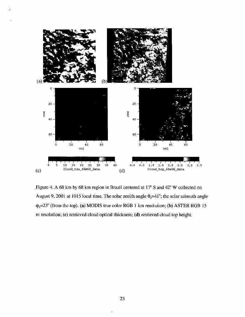
6. Illustration with MODIS data

To illustrate the above theory with observations, we have selected a 1 km spatial

resolution MODIS 68 km by 68 km broken cumulus cloud scene (Fig. 4a) from a less

polluted region in Brazil, centered at 17" S and 42" W. The data were acquired on August

9, 2001 at 10: 15 am local time. The solar zenith angle 8,=41°. This scene is part of the

International Comparison of 3D Radiative Transfer Codes (I3RC) phase 3 (Cahalan et al.,

2005) and has been used for the analysis of the retrieved droplet size by Marshak et al.

(2006) and for the radiative effects of broken clouds on aerosol retrievals by Wen et al.

(2007). Cloud fraction in the scene, Ac=0.4. The MODIS image is collocated with a high

spatial resolution (15 m) Advanced Spaceborne Thermal Emission and Reflection

Radiometer (ASTER) image (Yamagushi et al., 1998) plotted in Fig. 4b. The solar

azimuth angle <p,=23" (from upper right corner) as can be confirmed from the casting of

the shadows.

In panel (c) and (d) we have also added the retrieved cloud optical depth and

cloud top height at a 1 by 1 km resolution. While the retrieved 1 by 1 km cloud optical

depth is an operational MODIS product, the operational cloud top height retrievals have a

5 by 5 km resolution. To estimate the 1 by 1 km resolution of cloud top height, as in

Wen et al. (2007), we used the brightness temperature at 11 pm (MODIS band 31). As a

result, panels (c) and (d) will be served as the basic scenes for our illustration.

First, Fig. 5a shows the indicator function I(x,y) of the cloud optical depth field

from panel 4c. Cloud fraction, as a mathematical expectation of I defined in (7, will be

0.4. The right panel, Fig. 5b, is an indicator function of a realization of a simulated field

that has then the same correlation function K(x,y) as the measured one. As shown in

Appendix, to get K(x,y) we first estimated the covariance function K, defined in (8) and

then retrieved K(x,y) with the help of the Owen function (Prigarin et al., 2004).

Next we illustrate how distribution of cloud optical depth can be reproduced using

Eq. (12a). This is Model A which is, perhaps, better agrees with the results of

observations than model B (Prigarin and Marshak, 2005). Four realizations of cloud

optical depth distribution are plotted in Fig. 6. All of them have approximately the same

correlation function K(x,y) and probability density function g(7) as the original cloud

optical depth field shown in Fig. 5c . Figure 7 illustrates these five pdfs: the original one

and four realizations of cloud optical depth from Fig. 6.

Now we illustrate joint distribution of optical depth and cloud top height. Figure

8 shows a joint distribution function while Fig. 9 shows an example of two conditional

distributions F(hlz) for ~=3.5&0.5 and ~=10&1. The distributions of cloud top height h are

obviously different. Finally, Fig. 10 for the realization of cloud optical depth plotted in

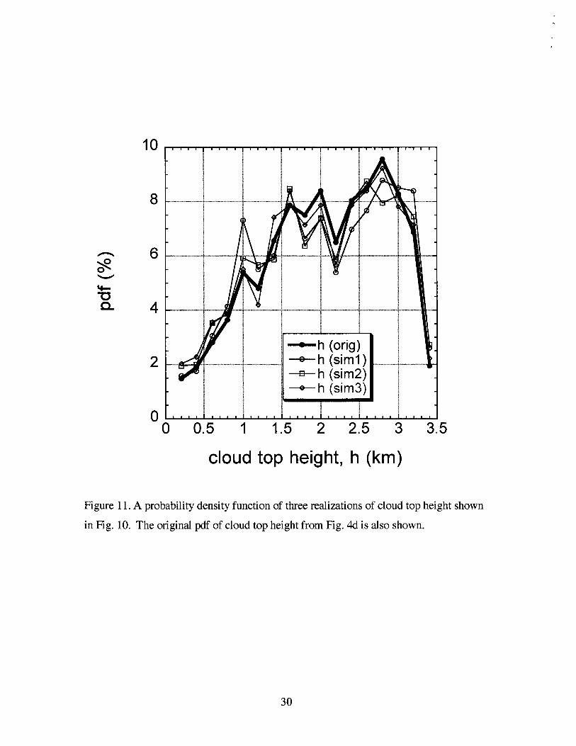
Fig. 6b shows three realizations of cloud top height. As we can see from Fig. 11 their

pdfs match (approximately) the original pdf of cloud top height from Fig. 4d.

7. Main steps of the model

Based on the above description, a software that generates realizations of cloud optical

depth and cloud top height from given observations have been developed and is freely

available for download from http://i3rc.gsfc.nasa.rrov/Public codes clouds.htm (click on

PDF-based stochastic cloud model). Note that at present, the software runs only on

Windows PCs.

Let us summarize here the main steps of the simulation procedure. Note that there are

only two input files: cloud optical depth z(x,y) and cloud geometrical thickness h(x,y) (as

shown in Figs. 4c and 4d). The main 11 steps are the following:

1. Read input file z(x,y) ;

2. Get cloud fraction A,, as in (7);

3. Find the truncation level d, as in (2);

4. Compute covariance function of the indicator field K,, as in (8);

5. Estimate correlation function K, as in Appendix;

6. Generate a Gaussian field, as in (1);

7. Modify the Gaussian field, as in (12);

8. Read input file h(x,y);

9. Calculate joint distribution of zand h fields, as in Fig. 8;

10. Calculate a conditional distribution matrix, as in (13);

11. Simulate a realization of the h-field that corresponds to a realization of the T-field

generated at step 7;

In the software, the first 7 steps are accomplished by the executable file Ox-sp-a-

s.exe. The input file is matrix ~(x,y). The output files are: a realization of cloud optical

depth field, estimated autocorrelation function of the indicator field, computed

autocorrelation function of the Gaussian field and histograms of the input and output

optical depth fields. The executable file DISTR-M2.exe estimates a joint distribution

function of two random fields z(x,y) and h(x,y). The output files of this program are joint

and conditional distributions (steps 8-10). For the last step, the executable file

X-Ysim.exe is used. It provides a realization of cloud top height field.

8. Summary

Cloud stochastic models proved to be an important tool to study 3D radiative effects

in clouds, especially in broken cumulus clouds (e.g., Barker and Davies, 1992, Evans,

1993, Marshak et al., 1998, Varnai, 2000, Evans and Wiscombe, 2004, Schmidt et al.

2007). Here we have provided a theoretical description of a simple algorithm that

generates realizations of two correlated stochastic two-dimensional (2D) cloud fields that

have similar statistical characteristics as given cloud fields. Each step of the algorithm

has been illustrated with two broken cumulus cloud fields: cloud optical depth and cloud

top height retrieved from MODIS. While most stochastic cloud models use Fourier

filtering of Gaussian signal to generate the required correlation (e.g., Schertzer and

Lovejoy, 1987; Evans, 1993; Di Giuseppe and Tompkins, 2003; Evans and Wiscombe,

2004; Hogan and Kew, 2005; Venema et al., 2006b), our algorithm is based on spectral

models of homogeneous random fields (Prigarin, 1995, 2001). A nonlinear

transformation of Gaussian functions (the method of inverse distribution function) allows

us to keep distribution function similar to the one of the first original field. Realizations

of the correlated second field are generated using a conditional distribution matrix.

This paper is accompanied by a software that has been just released and can be freely

downloaded from http://i3rc.gsfc.nasa.gov/Public codes clouds.htm. The software

generates a two-component cloud field and provides programs to simulate two-

dimensional distributions. The software contents a program (Ox-sp-a-s) that generates

realizations of a broken cloud field (X) with similar statistical characteristics

(autocorrelation, density, and indicator functions) as the first given sample, a program

(DISTR-M2) that estimates joint and conditional distributions for two given samples and

a program (X-Ysim) that simulates sample Y while the sample X is given. At present,

the software runs only on Windows PCs but will be later extended to other platforms.

Acknowledgments. Both S. Prigarin and A. Marshak have been supported by the NSF

Collaboration in Basic Science and Engineering (COBASE) travel grant. S. Prigarin has

been also supported by INTAS (Grant 05-1000008-SOU), RFBR (Grant 06-05-64484)

and the President's program Leading Scientific Schools (Grant NSh-4774.2006.1). A.

Marshak has been supported by the Department of Energy (under grant DE-A105

90ER61069 to NASA's GSFC) as part of the Atmospheric Radiation Measurement

(ARM) program and by NASA's Radiation Program Office (under grants 621-30-86 and

622-42-57). We thank Dr. Tamas Varnai for his help with testing the software and Dr.

Warren Wiscombe for stimulating the development of stochastic models of broken cloud

fields.

Appendix. Relations for covariance functions of a Gaussian random filed and its

indicators

Assume that v(x) is a homogeneous Gaussian random field on the plane with

mean zero and correlation function K(x,y)=E[v(x,y) v(0,0)]. Let us consider two indicator

fields with respect to a fixed level d:

0 for v(x,y)<d I(')(X,~)=

1 otherwise '

0 for lv(x,y)l<d (x,y)=

1 otherwise

These indicators correspond to Model A (la) and Model B (lb) introduced in Section 2.

In this Appendix we present basic relations between covariance functions of the random

field v(x,y) and its indicators (for details, see Prigarin et al., 2004). For covariance

functions K@)(x, y) =E [l(")(x,y) l@)(0,0)] we have

where

and

is the probability density of a two-dimensional Gaussian random vector with zero mean,

unit variance of the components and correlation coefficient p between the components.

To find the correlation function K(x,y) of the Gaussian random field for a quasi-

Gaussian model of broken clouds it is necessary to estimate function K(n)(x,y) that is the

covariance function of the cloud indicator field and to solve numerically equation (Al)

(n=l for Model A and n=2 for Model B). For computations it is reasonable to use the

following representations of (A2) in terms of Owen's function:

R(')(p) = @(-d)-2T(dya), R(')(~) =4@(-d)-4[T(d,a)+T(d, 1 la)], 644)

where 0 is the standard normal cumulative distribution function, a = ,/- and

1 a du ~ ( d , a ) = - j exp[-d2(l+u2)/2]-

2n 0 1+u2 (A51

is Owen's function.

References

Ackerman, A. S., 0. B. Toon, and P. V. Hobbs, 1995: A model for particle microphysics, turbulent mixing, and radiative transfer in the stratocumulus-topped marine boundary layer and comparisons with measurements. J. Atmos. Sci., 52, 1204- 1236.

Barker, H. and J. A. Davies, 1992: Solar radiative fluxes for stochastic, scale-invariant broken cloud fields. J. Atmos. Sci., 49, 1 1 15- 1 126.

Cahalan, R. F., 1994: Bounded cascade clouds: Albedo and effective thickness. Nonlinear Processes in Geoph., 1, 156-1 67.

Cahalan R.F, L. Oreopoulos, A. Marshak, K.F. Evans, A.B. Davis, R. Pincus, K. Yetzer, B. Mayer, R. Davies, T.P. Ackerman, H.W. Barker, E.E. Clothiaux, R.G. Ellingson, M.J. Garay, E. Kassianov, S. Kinne, A. Macke, W. O'Hirok, P.T. Partain, S.M. Prigarin, A.N. Rublev, G.L. Stephens, F. Szczap, E.E. Takara, T. V h a i , G. Wen, and T.B. Zhuravleva, 2005. The International Intercomparison of 3D Radiation Codes (I3RC): Bringing together the most advanced radiative transfer tools for cloudy atmospheres. Bulletin Amer. Meteor. Soc. (BAMS), 86, 1275- 1293.

Di Giuseppe, F., and A.M. Tompkins, 2003: Effect of spatial organization on solar radiative transfer in 3D idealized stratocumulus cloud fields. J. Atmos. Sci., 60, 1774- 1794.

Evans, K.F., 1993: A general solution for stochastic radiative transfer. Geoph. Res. Lett., 20,2075-2078.

Evans, K.F., and W.J. Wiscombe, 2004: An algorithm for generating stochastic cloud fields from radar profile statistics. Atmos. Res., 72, 263-289.

Evans, K.F., A. Marshak, and T. Varnai, 2007. The potential for improved cloud optical depth retrievals from the multiple directions of MISR. J. Atmos. Sci., (submitted Sep 2007).

Gentle J.E., 2003 Random Number Generation and Monte Carlo Methods, Springer, Yd ed., 381 p.

Gikhman 1.1. and A.V. Skorokhod, 1977: An Introduction to the Theory of Random Processes. Nauka, Moscow [in Russian].

Hogan, R. J. and S. F. Kew, 2005: A 3D stochastic cloud model for investigating the radiative properties of inhomogeneous cirrus clouds. Q. J. R. Meteorol. Soc., 131, 2585-2608.

Marshak, A., A. Davis, R.F. Cahalan, and W.J. Wiscombe, 1994: Bounded cascade models as non-stationary multifractals. Phys. Rev. E, 49,5549.

Marshak, A., A. Davis, W.J. Wiscombe, W. Ridgway, and R.F. Cahalan, 1998: Biases in shortwave column absorption in the presence of fractal clouds. J. Climate, 11,43 1 - 446.

Marshak, A., S. Platnick, T. Vhrnai, G. Wen, and R. F. Cahalan, 2006. Impact of 3D radiative effects on satellite retrievals of cloud droplet sizes. J. Geophys. Res., 111, DO9207 doi: 10.1029/2005JD006686.

Ogorodnikov, V.A. and S.M. Prigarin, 1996: Numerical Modelling of Random Processes and Fields: Algorithms and Applications, VSP, Utrecht, the Netherlands, 240 p.

Prigarin S.M., 1995: Spectral models of random fields and their applications. Advances in modelling and analysis, A, 29,2, 39-5 1

Prigarin, S.M., 2001: Spectral Models of Random Fields in Monte Carlo Methods, VSP, Utrecht, 198p.

Prigarin, S. M., B.A. Kargin, and U.G. Oppel, 1998: Random fields of broken clouds and their associated direct solar radiation, scattered transmission, and albedo. Pure and Applied Optics, A, 7, 1389- 1402.

Prigarin, S.M., A. Martin, G. Winkler, 2004: Numerical models of binary random fields on the basis of thresholds of Gaussian functions, Siberian J. of Num. Math., 7, 165- 175.

Prigarin, S., and A. Marshak, 2005. Numerical model of broken clouds adapted to observations. Atmos. and Oceanic Optics, 18,256-263.

Prigarin, S. and A. Marshak, 2007. Simulation of vector semi-binary homogeneous random fields and modeling of broken clouds. Siberian J. Numeric. Anal., (submitted July 2007).

Scheirer R. and S. Schmidt, 2005: CLABAUTAIR: A new algorithm for retrieving three- dimensional cloud structure from airborne microphysical measurements. Atmos. Chem. Phys. 5: 2333-2340.

Schertzer, D., and S. Lovejoy, 1987: Physical modeling and analysis of rain and clouds by anisotropic scaling multiplicative processes. J. Geophys. Res., 92,9693-9714.

Schmidt, K.S., V. Venema, F. Di Giuseppe, R. Scheirer, M. Wendisch, and P. Pilewski., 2007: Reproducing cloud microphysics and irradiance measurements using three 3D cloud generators. Q.J.R. Meteorol. Soc., 133,765-780.

Sveshnikov, A. A., 1968. Applied Methods in Random Function Theory. Nauka, Moscow, 463 pp. (in Russian)

VArnai, T., 2000: Influence of three-dimensional radiative effects on the spatial distribution of shortwave cloud reflection. J. Atmos. Sci., 57,216-229.

Venema, V., S. Bachner, H.W. Rust, and C. Simmer, 2006a: Statistical characteristics of surrogate data based on geophysical measurements, Nonlin. Proc. Geophys., 13, 4 4 9 4 .

Venema, V., S. Meyer, S.G. Garcia, A. Kniffka, C. Simmer, S. Crewell, U. Lohnert, T. Trautmann and A. Macke, 2006b: Surrogate cloud fields generated with the iterative amplitude adapted Fourier transform algorithm, Tellus., 58A, 104-120.

Voss, R., 1985. Random fractal forgeries. In R.A. Earnshaw, editor, Fundamental Algorithms in Computer Graphics, pages 805-835. Springer-Verlag.

Wen, G., A. Marshak, R.F. Cahalan, L.A. Remer, and R.G. Kleidman, 2007. 3-D aerosol-cloud radiative interaction observed in collocated MODIS and ASTER images of cumulus cloud fields, J. Geophys. Res., 112, D13204, doi: 10.1029/2006JD008267.

Zuev V.E. and G.A. Titov, 1995: Radiative transfer in cloud fields with random geometry. . J Atmos. Sci., 52, 176- 190.

FIGURES

- clouds

Illurtratisn of Model A

illustration of Model 6

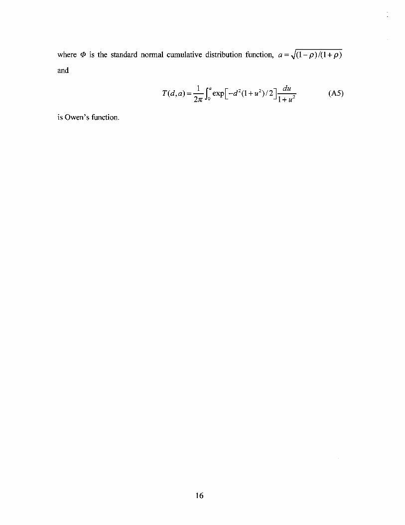
Figure 1. A schematic illustration of models A and B. H, is a constant cloud base, d is a

cutting threshold level.

--. -mc k= l for model B

Figure 2. Number of clouds per unit area, m,, as a function of cloud fraction A, for both

models A and B .

Fig. 3. Configuration of cloud fields (300*300 km) for model A (left) and model B

(right) on the basis of a Gaussian random field with correlation function J, for the same

cloud fraction A,=0.58 (p=0.5; d= - 0.20 for model A, and d=0.55 for model B).

0 2 0 4 0 60 col

0 20 40 6 0 col

Figure 4. A 68 km by 68 km region in Brazil centered at 17" S and 42" W collected on

August 9,2001 at 1015 local time. The solar zenith angle 8,=41°; the solar azimuth angle

cpO=23" (from the top). (a) MODIS true color RGB 1 km resolution; (b) ASTER RGB 15

m resolution; (c) retrieved cloud optical thickness; (d) retrieved cloud top height.

Figure 5. Indicator functions I(x,y) of a cloud field: red is cloud (I=l) while black is a

cloud free area (I=O). Cloud fraction Ac=0.4. (left) 68 by 68 km MODIS image centered

at (17. lo S,42.16OW) acquired on August 9,2001. (right) a realization of a simulated

field.

Figure 6. Four realizations of cloud optical de

function K(x,y) and histogram g(z) as the one i

Fig. 4c.

,pth; all of them have the same correlation

n Fig. 4c. Color scale is the same as in

optical depth

Figure 7. The original histogram g(2) and four other histograms that correspond to four

realizations of cloud optical depth shown in Fig. 6.

0 1 2 3 cloud t o p height (krn)

0.000 0.002 0.004 0.006 0.008 0.010 j o i n t t a u - height d i s t r i b u t i o n

Figure 8. Joint distribution of the given cloud optical depth and cloud top height fields.

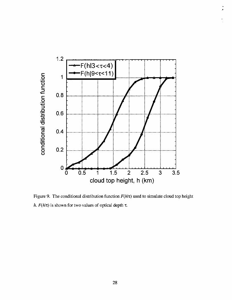
Figure 9.

h. F(hlz)

0 0.5 1 1.5 2 2.5 3 3.5 cloud top height, h (km)

. The conditional distribution function F(hlz) used to simulate cloud top

is shown for two values of optical depth z.

height

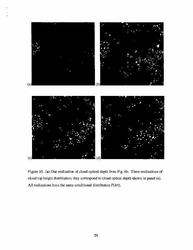
Figure 10. (a) One realization of cloud optical depth from Fig. 6b. Three realizations of

cloud top height distribution; they correspond to cloud optical depth shown in panel (a).

All realizations have the same conditional distribution F(hlz).

cloud top height, h (km)

Figure 11. A probability density function of three realizations of cloud top height shown

in Fig. 10. The original pdf of cloud top height from Fig. 4d is also shown.