A simple model of the â€joint effect of baroclinicity and

Journal of Marine Research, 53, 211-230,199s

A simple model of the ‘joint effect of baroclinicity and relief’ on ocean circulation

by Rick Salmon’ and Rupert Ford1,2

ABSTRACT We offer a simple model for studying the joint effect of baroclinicity and relief (jebar) on

large-scale ocean circulation, based upon the planetary geostrophic equations. Applying a Galerkin approximation to the buoyancy equation, and asssuming that the temperature diffusion and vertical stratification are weak, we obtain a simple relation between the ocean temperature and the streamfunction + for the vertically-averaged horizontal transport. Substituting this relation back into the vertically-averaged vorticity equation yields a single, generally nonlinear equation for JI, in which jebar corresponds to a clockwise ‘advection’ of $ along the continental slope (for the realistic case of temperature increasing with $I). Numerical solutions resemble those obtained by Salmon (1994) using a more accurate model, and provide a physically transparent explanation for the northward excursion of the Gulf Stream along the western continental slope observed in the previous study.

1. Introduction

When the pressure at the ocean bottom varies along isobaths, the water column feels a ‘bottom torque.’ It is customary to divide this bottom torque into two components. The first component is the total torque that would occur if the fluid were completely homogeneous. The second component represents the adjustment to the torque arising from density variations within the fluid, through the hydrostatic dependence of pressure on fluid density. This second component is also called jebar, for joint efict of baroclinicity and relie$ In ocean circulation models based upon the geostrophic approximation, jebar represents the sole feedback of the density field on the equation determining the depth-averaged flow.

A previous paper (Salmon, 1994; hereafter S94) described numerical solutions of a particularly simple ocean circulation model based upon an abridgment of the planetary geostrophic equations, (2.1-2). The S94 model comprises two coupled, second-order equations in two dependent variables: the streamfunction \Ir(x, y) for

1. Scripps Institution of Oceanography, La Jolla, California, 92093-0225, U.S.A. 2. Present address: Dept. of Mathematics, Imperial College, 180 Queen’s Gate, London, SW7 2BZ,

United Kingdom. 211

212 Journal of Marine Research 15372

the depth-integrated flow, and the ocean surface temperature T(x,~).~ The +equation, an equation for the vertically-integrated vorticity, contains a T-term corresponding to jebar. The T-equation, an equation for the vertically-averaged temperature, contains a +-term corresponding to the advection of temperature by the vertically- averaged flow. The S94 equations also contain an arbitrary projile function, which controls the dependence of temperature on potential vorticity, and, thereby, the dependence of temperature on depth. If this profile function is chosen to be a step- (i.e. Heaviside) function, then the equations reduce to the conventional equations for two immiscible, homogeneous layers. The S94 equations were therefore called generalized two-layer equations (GTLE). However, smoother choices of profile function proved both more realistic and numerically convenient.

The GTLE are certainly one of the simplest sets of dynamical equations that could be used to study the effect of jebar on the depth-averaged flow, and the numerical solutions described in S94 show that this effect is especially significant along the western continental slope, where jebar causes a large northward excursion of the Gulf Stream along the continental slope. However, the GTLE, while simple, are by no means transparent, and real physical understanding of the most prominent GTLE results probably requires even more drastic simplifications. In this paper, we offer one such simplification.

Our starting point, as in S94, is the planetary geostrophic equations. Assuming that the ocean temperature varies exponentially with depth, we obtain, by a Galerkin method, a pair of IJJ- and T-equations (3.5, 3.13) similar to, but somewhat simpler than, the GTLE. Then, assuming that thermal forcing and diffusion are everywhere less important than temperature advection, and supposing that the vertical derivative of temperature is small, we ‘solve’ the temperature equation, obtaining a simple expression for the temperature as a function of the transport streamfunction. In the simplest case, of temperature assumed independent of depth, our solution is

T = F(4), (1.1)

where F( ) is an arbitrary function, continuous but not necessarily single-valued. In the more realistic case of small but nonzero vertical stratification we obtain the generalization (3.21) of (l.l), which includes the effect of westward propagation of temperature. Then, substituting (1.1) or (3.21) back into the jebar term in the +-equation, we obtain a single, generally nonlinear equation for $. We call this single equation the toy model, because it relies on approximations that certainly cannot be strictly justified.

However, numerical solutions of the toy model reproduce some of the important features of the GTLE solutions described in S94. Equally important, the toy-model equation is sufficiently simple-for linear F( ), it is actually linear-that the physics

3. More precisely, S94 used a temperature variable S(x, y), related to the surface temperature 7&y) by T = O(S), where O( ) is a prescribed function.

19951 Salmon & Ford: JEBAR 213

behind these features is transparent, and one understands immediately why (for example) the jebar must lead to a northward over-shoot of the Gulf Stream along the western continental slope. The toy model apparently succeeds because its fundamen- tal assumption-that the ocean temperature is, to a first approximation, constant on lines of constant transport streamfunction +-is most nearly correct near the western continental slope, where jebar is also most significant. However, we stress that the toy model is not a tool for accurately simulating the real ocean. Instead, we regard the toy model as a ‘thinking tool,’ intended to enlarge our intuition about the interaction between flow and topography, and to be replaced by something better as that intuition improves.

2. Toy model for depth-independent temperature

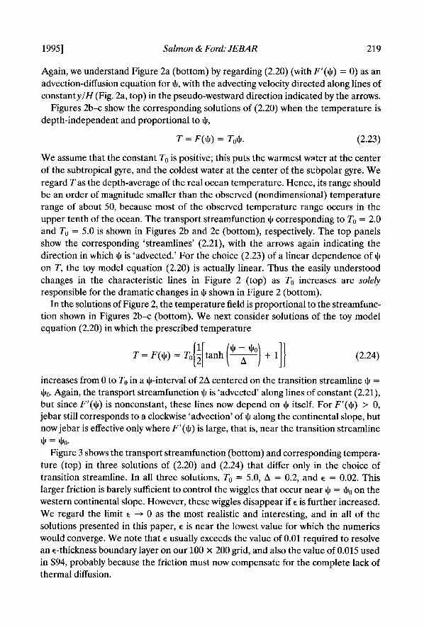
In the usual (nondimensional) notation, the planetary geostrophic equations (PGE) are

(2.1)

and

8, + z&3, + ~0, + we, = Q + KV@. (2.2)

Here, (u, v, w) is the velocity in the (x, y, z) direction, corresponding to (east, north, up);f = y is the Coriolis parameter; 4 is the pressure, and 8 the buoyancy. We will call t3 the temperature. The constants E and K are coefficients of Rayleigh friction and temperature diffusion, respectively. Q is the diabatic heating, and (TX@, y, z), +‘(x, y, 2)) is thepresctibed horizontal stress, assumed nonzero only near the ocean surface. Our notation is V3 = (i&, a,, &) and V = (a,, a,). For a more complete discussion of (2.1-2) including the philosophy behind the Rayleigh friction, refer to S94 and earlier papers cited therein. The nondimensionalization of (2.1-2) is the same as in S94, and will be explained again later on.

As previously shown, the planetary geostrophic equations (2.1-2) are well-posed with respect to temperature boundary conditions of prescribed temperature (or heat flux) at all boundaries, and velocity boundary conditions of no-normal-flow at the ocean surface,

w=o at2 = 0, (2.3)

214 Journal of Marine Research [53,2

and bottom

w = -uH, - vH~ at z = -H(x, y), (2.4)

provided that the ocean depth H vanishes smoothly at the coastline. (If any part of the boundary is vertical, then the vertical momentum equation (2.1~) must also contain a Rayleigh friction term.) The temperature equation (2.2) and temperature boundary conditions are used to step 9 forward in time. Then, at the new time, the velocity components (u, v, w) are instantaneously determined by the Cl-field, the linear equations (2.1), and the boundary conditions, as follows. First, the two- dimensional elliptic equation

and boundary condition + = 0 determine the transport streamfunction $, defined by

(2.6)

where u = (u, v) is the horizontal velocity. Here,

yfc - 760’ W(x, y) = curl

( 1 H , (2.7)

and r’f”, 76”’ are the prescribed stress at the ocean surface and bottom, respectively. The temperature enters (2.5) through

With + determined by (2.5), the velocity field is given by

and

(2.8)

(2.9)

where u’, the departure of the horizontal velocity from its vertical average, is determined by the thermal wind equations,

au’ - = yp& [-ye, - d3, + y7Y, + E7X,] a.2

avr 1 - = - [+y@ - 4, - y7x, + ET&] a.2 y* + 2

(2.11)


and

s

0 g’dz = 0.

In S94 we considered PGE solutions of the special form

l.3 = 0 i ; + S(x,y, t)

i

(2.12)

(2.13)

where O( ) is an arbitrary profile function, and the evolution equation for the new dependent variable S(x, y, t) results from substituting (2.13) back into the PGE. The significance of (2.13) is that it leads to an exact reduction of the PGE from three to two space dimensions in the ideal limit of no forcing and dissipation (T=Q=O=E=K).T~ e ansatz (2.13) is equivalent to the assumption that surfaces of constant temperature and potential vorticityy0, coincide (Needler, 1971). In the general case with forcing and dissipation (or if the ocean includes the equator, y = 0), the ansatz (2.13) must be slightly modified, and the resulting S94 equations then have the status of a Galerkin approximation. If the arbitrary function O( ) is chosen to be a step function, then these equations reduce to the conventional equations for two immiscible layers; hence the name generalized two-layer equations (GTLE). For complete details, refer to S94.

Numerical solutions of the GTLE described by S94 showed interesting and perhaps realistic features, especially along western continental slopes, where the second, so-called jebar, term in (2.5) significantly affected the transport. However, the numerical solutions of S94 had two shortcomings. First, the ideal geometry (a rectangular ocean with continental slopes and shelves of uniform width) made it difficult to compare the results with observations of the real ocean, which has a very irregular shape. And second, the GTLE dynamics, while much simpler than even the full PGE, were still too complicated for a completely satisfactory interpretation of the solutions. The need for an even simpler dynamics than GTLE is readily apparent when one confronts the enormous but seemingly unavoidable task of incorporating real bathymetry, while keeping the ultimate goal of physical understanding.

In this paper, we offer an abridgment to the GTLE based upon the somewhat unrealistic assumptions that the temperature stratification Cl,, thermal forcing, and thermal diffusion are all small. This abridgment, which we call toy dynamics, leads to a single, nonlinear elliptic equation for the transport streamfunction $(x, y). This streamfunction equation can easily be solved by a numerical relaxation method, and the solutions are easy to understand. More importantly, solutions of the toy model bear a surprising resemblance to the GTLE solutions described by S94. Thus, it seems that much of the physics of the GTLE can be understood by appealing to the simpler toy dynamics.

First, suppose that

0 = W,Y, t), (2.14)


where T is a z-independent function to be determined. The general +-equation (2.5) becomes

+;J(T,H)=W+

The velocity field determined by (2.9-12) is

(2.15)

(2.16)

where O(E, T) stands for terms containing the Rayleigh friction or prescribed stress. Substituting (2.14) and (2.16) into (2.2), we obtain

Hz + J(+> 0 = O(E, 7, Q, K),

in which many terms are absent because 0, = 0, and because the thermal wind (the second term in (2.16a,b)) is tangent to the isotherms.

Now, we are interested in the case of small forcing and dissipation. Furthermore, experiments with the full PGE and with the GTLE show that the solutions tend toward steady states. Thus, to leading order, (2.17) is

with solution

J(h T) = 0 (2.18)

T = F(e). (2.19)

We regard F( ) as an arbitrary function; a better interpretation would be that F( ) is determined, at higher order, by the small (arbitrary) forcing and dissipation. With (2.19) the $-equation (2.15) becomes

(2.20)

As in previous papers, we regard (2.20) as an ‘advection-diffusion’ equation for the scalar $. Now, however, the ‘streamfunction’ for the advecting velocity, viz.

contains a second term corresponding to the advection of IJJ along isobaths at a speed


Y=O

Figure 1. The ocean basin topography used for all solutions. The ocean depth varies between 0 and 1, and vanishes smoothly at the western, northern, and eastern boundaries. The southern, equatorial boundary is open.

proportional to the bottom slope. If, as we assume below, F’(IJJ) > 0 (to give the largest values of T where 4 is largest, at the center of the subtropical gyre), then this second term corresponds to a ‘velocity field’ that sweeps IJJ clockwise along the continental slope in the northern hemisphere. As we see next, this tendency, so simply understood from (2.20), qualitatively explains much of the jebar effect observed in the experiments described by S94.

We use the same non-dimensionalization of variables as in S94. Briefly, horizontal distances are in units of the basin width (4000 km), vertical distances in units of the maximum depth (4 km), and horizontal velocities in units of .2 km/day to make a realistic Sverdrup transport (30 Sverdrups) correspond to + = O(1). The units of buoyancy are then .02 cm2/sec, so that the observed density range in the ocean corresponds to a range in nondimensional 8 of about 50-100.

We use the same ocean basin topography (Fig. 1) as in S94. The ocean depth vanishes smoothly at coastlines on the western, northern, and eastern boundaries. The southern, equatorial boundary is open. To ensure sufficient numerical resolu- tion in regions of steeply sloping topography, we greatly exaggerate the widths of the continental shelves and slopes; altogether they occupy more than half the total basin area. The prescribed two-gyre wind curl,

W&Y) = -& . sin(;y)cos(ty), (2.22)

is the same as in S94. Figure 2a (bottom) (which is identical to Figure 2b in S94) shows the transport streamfunction in the case of homogeneous fluid, that is, the solution of (2.20) with F(+) = 0 and E = 0.015, the same friction value used in S94.

a

I

Figure 2. The transport streamfunction + (bottom) in three solutions of the toy model equation (2.20) with depth-invariant temperature given by the linear relation (2.23). All three solutions have E = 0.015, and differ only in the value of the coefficient To in (2.23): (a) To = 0.0 (homogeneous fluid); (b) To = 2.0; (c) To = 5.0. Thus, the sequence (a-c) corresponds to increasing temperature contrast within the fluid. Darker contours correspond to larger values of ~JJ, and extremal values are shown. The top panels show the corresponding ‘streamfunction’ (2.21) for the ‘flow ’ ‘advecting’ + in (2.20) with ‘flow’ direction indicated by the arrows.


Again, we understand Figure 2a (bottom) by regarding (2.20) (with F’(+) = 0) as an advection-diffusion equation for $, with the advecting velocity directed along lines of constantylH (Fig. 2a, top) in the pseudo-westward direction indicated by the arrows.

Figures 2b-c show the corresponding solutions of (2.20) when the temperature is depth-independent and proportional to I&,

T = F(+) = T&. (2.23)

We assume that the constant To is positive; this puts the warmest water at the center of the subtropical gyre, and the coldest water at the center of the scbpolar gyre. We regard T as the depth-average of the real ocean temperature. Hence, its range should be an order of magnitude smaller than the observed (nondimensional) temperature range of about 50, because most of the observed temperature range occurs in the upper tenth of the ocean. The transport streamfunction \Ir corresponding to To = 2.0 and To = 5.0 is shown in Figures 2b and 2c (bottom), respectively. The top panels show the corresponding ‘streamlines’ (2.21), with the arrows again indicating the direction in which + is ‘advected.’ For the choice (2.23) of a linear dependence of $ on T, the toy model equation (2.20) is actually linear. Thus the easily understood changes in the characteristic lines in Figure 2 (top) as To increases are solely responsible for the dramatic changes in $ shown in Figure 2 (bottom).

In the solutions of Figure 2, the temperature field is proportional to the streamfunction shown in Figures 2b-c (bottom). We next consider solutions of the toy model equation (2.20) in which the prescribed temperature

T = F(e) = To I’[ (?)+11) 2 tanh (2.24)

increases from 0 to To in a +-interval of 2A centered on the transition streamline + = $,. Again, the transport streamfunction IJ is ‘advected’ along lines of constant (2.21), but since F’(+) is nonconstant, these lines now depend on I/J itself. For F’(Q) > 0, jebar still corresponds to a clockwise ‘advection’ of IJJ along the continental slope, but now jebar is effective only where F’(e) is large, that is, near the transition streamline 31 = *o-

Figure 3 shows the transport streamfunction (bottom) and corresponding temperature (top) in three solutions of (2.20) and (2.24) that differ only in the choice of transition streamline. In all three solutions, To = 5.0, A = 0.2, and E = 0.02. This larger friction is barely sufficient to control the wiggles that occur near + = +. on the western continental slope. However, these wiggles disappear if E is further increased. We regard the limit E + 0 as the most realistic and interesting, and in all of the solutions presented in this paper, E is near the lowest value for which the numerics would converge. We note that E usually exceeds the value of 0.01 required to resolve an e-thickness boundary layer on our 100 x 200 grid, and also the value of 0.015 used in S94, probably because the friction must now compensate for the complete lack of thermal diffusion.

Journal of Marine Research

a b

w

Figure 3. The streamfunction $ (bottom) and temperature T (top) in three solutions of the toy model equation (2.20) with depth-invariant temperature given by (2.24). In all three solutions E = 0.02, To = 5.0 and A = 0.2. The solutions differ only in the location of the temperature transition line: (a) +a = 0.0 (b) $0 = -0.12 (c) $0 = -0.25. The transition thus occurs on a progressively more subpolar streamline in the sequence (a-c).

In the solution of Figure 3a, the temperature transition occurs on the streamline +0 = 0 that divides the two wind gyres. In Figures 3b (+0 = -0.12) and 3c (+0 = -0.25) the transition occurs on progressively more subpolar streamlines, and the cold water is increasingly confined to the center of the subpolar gyre. By the same

199.51 Salmon & Ford: JEBAR 221

reasoning as above, the relatively southern transition in Figure 3a ‘advects’ positive values of JI northward along the western continental slope, causing a large penetration of warm, Gulf Stream water into the subpolar region. In fact, Figure 3a resembles Figure 2c (which had the same size temperature range) rather closely. But in the more northerly transitions of Figures 3b-c, this penetration is weaker, and in Figure 3c, jebar ‘advection’ acts principally to counteract the southward ‘advection’ of low subpolar G-values along lines of constant y/H, thus separating the gyres, inhibiting the c-diffusion of + between them, and leading to a stronger total transport in both gyres.

Despite the almost schematic simplicity of the toy model, Figures 2 and 3 qualitatively resemble the solutions of the much more realistic GTLE described in S94. See especially Figures 3 and 11 of S94, which exhibit the same northward overshoot of the subtropical western boundary current (although in shallower water, where the boundary condition on \cI forces the toy-model temperature to be nearly uniform, and jebar to be weak.)

Our assumption (2.14) of a vertically uniform temperature field is of course too severe; it leads to a temperature equation, (2.17), without a westward propagation term. However, in many of the GTLE solutions described in S94, westward propagation contributed importantly to the ‘characteristic velocity’ of the temperature equation, especially in the subtropical gyre, where the relatively thick warm-water layer and relatively small Coriolis parameter yielded a relatively large internal Rossby-wave speed. In the next section, we show how the steps leading up to (2.19) can be generalized to cover the case of a small but nonvanishing temperature stratification, thereby including westward temperature propagation in the toy-model physics.

3. The case of non-vanishing stratification

Now suppose that

q-&y, z, t> = w, y, t)@(z),

where O(z) is a prescribed function of depth, with the properties

(3-l)

O(0) = 1 and O’(z) 2 0 (3.2)

so that T(x, y, t) is the surface temperature, and the fluid is statically stable. The case (2.14) of vertically uniform temperature corresponds to the choice O(z) = 1. We now show that if O’(z) is nonzero but small, then an extension of the reasoning given in Section 2 generalizes the simple relation (2.19) between T and + to (3.21), which includes the effect of westward temperature propagation.

With (3.1) (2.8) becomes

y=-- s _oHzB dz = Tl?(H), (3.3)

222

where


r(H) = - J~~ZO(Z) dz,

and the general +-equation (2.5) becomes

W) ,,J(T,H) = W-V.

[53,2

(3.4)

(3.5)

Now, unlike (2.13) and (2.14), the ansatz (3.1) is not precisely consistent with the ideal PGE. That is, we cannot now obtain an exact, z-independent equation for T(x, y, t), even in the case of vanishing forcing and dissipation. Instead, as in S94, we determine T&y, t) by requiring that the temperature equation be satisfied in the vertical average, i.e. that

(3.6)

The horizontal velocity is now

t-YT, - GYT, - ETJ + O(T), (3.7)

where O(r) stands for terms proportional to the stress, and

G(z,H) = fHO(z’)dz’ +;s_ohz@(z)dz

ds the solution to

t-9

dG z = O(z), j-_“, G dz = 0. (3.9)

Then

s ww

-“, ue dz = TW)HJ~, 4~x1 + y2 (-yT,- eT,,yT, - ETA) + O(T), (3.10)

where

and

P(H) = +j s_“, O(z) dz (3.11)

R(H) = s_“, O(z)G(z, H) dz. (3.12)


Note that P(H)T is the vertically-averaged temperature. The vertically-integrated temperature equation (3.6) becomes

HZ’(H) $; + J($, P(H)T) + TJ

(3.13)

When O(z) = 1, thenP(H) = 1, R(H) = 0 and l?(H) = H2/2; and (3.13) reduces to (2.17).

The third term in (3.13) which has no counterpart in (2.17), causes a pseudo- westward propagation of T along lines of constantyR(H)l(y2 + l ‘). The propagation speed is proportional to T itself, leading to wave steepening and the possibility of shocks, as predicted by Dewar (1991) and noted in the numerical solutions of S94. When temperature shocks are present, the dissipation terms on the right-hand side of (3.13) are of course indispensable. However, in our further approximations, which are based upon the assumption that O’(z) is small, and are analogous to the approximations leading to (2.19) above for the case O(z) = 1, we will discard the forcing and dissipation terms on the right-hand side of (3.13), and also remove the possibility of shocks, while retaining some of the pseudo-westward propagation of T. But first we made an ad hoc modification to (3.13) that simplifies the dynamics at very low latitude.

Fory near E, the third term in (3.13) is large, but so is the first of the temperature diffusion terms on the right-hand side. Since further progress requires the neglect of all terms on the right-hand side of (3.13), we also modify the third term in (3.13) by replacingyl(y2 + e’) with l/(y + 6) w h ere 6 is a small fraction of the total basin length. This replacement, which is ad hoc, has the effect of capping the internal Rossby wave speed at its y = 6 value. Of course, it would be more graceful to avoid the equatorial near-singularity in the temperature equation by considering a model ocean with a southern boundary at y z=- E, 6. However, as E + 0, solutions of the $-equation (3.5) depend sensitively on the geometry of its characteristic lines of constant H/y. In the unrealistic case of a southern coastal boundary, the H/y-lines comprise a set of closed curves, and as explained by Kawase (1993) and in S94, the streamfunction IJJ differs markedly from the more realistic case in which the ocean extends to the equator, with characteristic lines as shown in Figure 2a (top).

After the modifications noted above, and again assuming steady state, the temperature equation (3.13) becomes

J($, P(H)T) + J

Again, the first term represents the advection of temperature by the depth-averaged


flow, while the second term propagates T pseudo-westward, now along lines of constant R(H)I(y + S), at a speed proportional to T itself.

Now suppose that O’(z) is small. Then

P(H) = 1 + wtw, R(H) = IJW), (3.15)

where TV, is a small parameter that measures O’(z). The temperature equation (3.14) can be rewritten

J(k W + VP)) + J ( -$.)=o. T, P

But, to within an error of order k2, (3.16) is the same as

, T(1 + cup) = 0.

That is,

with implicit solution

TP(H) = F

(3.16)

(3.19)

where F( ) is an arbitrary function. On the other hand, suppose that the ocean bottom is flat, H = constant, but that

the stratification parameter TV, is not necessarily small. Then P(H) and R(H) are constants, and (3.14) is equivalent to

RT 4~ - ty + 6jp > TP = 0,

with implicit solution

WW * - ty + s)p(H) (3.21)

where, again, F is an arbitrary function. But to within an error of order l~,~, (3.20) is the same as (3.18). Thus (3.20) holds if either the stratification t.~ is small, or if the bottom is flat. Hence, we regard (3.20) as a somewhat better approximation than (3.18). Note, in particular, that (3.18) under-estimates (by a factor of P) the speed of westward temperature propagation in the flat-bottomed interior ocean. However, (3.21) holds only if (3.20) is everywhere satisfied, and we must therefore regard weak stratification, t.~ -K 1, as the necessary condition for (3.21), just as it is for (3.19).


In the limit l.r, += 0 of vanishing stratification, P + 1, R -+ 0, and (3.21) reduces to (2.19). For nonvanishing stratification, (3.21) states that the depth-averaged temperature TP is constant along characteristic lines of constant

(3.22)

Again, the first term in (3.22) represents advection by the depth-averaged flow; the second term represents the pseudo-westward temperature propagation.

In the solutions described below, we take

O(z) = ehr,

where A is a constant. Then, with p = AH,

1 - e-p

P(H) = 7 N CL b2

1 -z+z- ***,

R(H)=2H25 1

l-coshF+Zksinhu.

and

21J3 3j.L5 - 2H2e-p $ + -gj- + sr +

1. .

T(H) = 5 [l - (1 + b)e-k] N Hz

We solve

I’(H) ,,J(T,H) = W-V.

(3.23)

(3.24)

(3.25)

1 (3.26)

(3.27)

with T determined by (3.21) for several choices of F( ). Figure 4 shows the depth parameters P(H), R(H), and T(H) as functions of the stratification parameter b z )LH. The maximum in R near CL = 1 corresponds to the well-known fact that the internal Rossby speed is largest when the temperature transition occurs near mid-depth.

We next present solutions of (3.5) and (3.21) with h = 1, the largest value for which the approximations leading up to (3.21) can be defended. However, when h f 0, no single-valued F( ) can be realistic: Where $ dominates the argument (3.22), it would be reasonable to choose a monotonically increasing F( ), so that the warmest water lies in the subtropical gyre, as in Section 2. However, in the eastern ocean, the second term in (3.22) dominates, so that a monotonically increasing F( ) would lead to cold water near the equator, and warmer water in the north. This temperature reversal


Figure 4. The three functions P(H), R(H) and T(H) that appear in the toy model, shown as functions of the parameter k = AH, where H is the ocean depth and A-* is the decay-depth for temperature.

would be most problematic near the equator, where the second term in (3.22) is largest. To avoid this difficulty, we assume that the arbitrary function F(c) in (3.21) is multi-valued. In particular, we assume that

F(c) = To 5 tanh (‘[ (?)+1]) (3.28)

everywhere outside an equatorial region in which the lines of constant 5 enter and leave at the southern boundary but do not extend into the subpolar region. Within this equatorial region, we let the depth-averaged temperature TP be uniform at the value it has on the bounding contour (a line of constant .Q of this region. The toy-model temperature equation (3.20) is then everywhere satisfied, and the temperature (but not its derivative) is everywhere continuous. The warmest water still occurs at the center of the subtropical gyre, but the water near the equator is not unrealistically cold.

To see how this works, refer to Figures 5 and 6. Figure 5 shows the depth-averaged temperature (3.21) (left) and the argument 5 defined by (3.22) (right) in the toy-model solution corresponding to Figure 6b. In most of Figure 5, the arbitrary function F(c) is given by (3.28) with TO = 5.0, A = 0.2 and .& = -0.2. However, in the southern region described above, we take the depth-averaged temperature TP to be uniform. The depth-averaged temperature is still warmest in the western subtropical


TP w- $)P

Figure 5. The depth-averaged temperature (left) and the quantity (3.29) in the solution presented in Figure 6b. According to the toy-model temperature equation (3.20), the Jacobian of these two quantities must vanish.

ocean, where, in the real ocean, the warm-water layer is thickest. The equatorial depth-averaged temperature is cooler, but not unrealistically cold.

Figure 6 shows three stratified (A = 1.0) solutions in which the temperature equation is satisfied in the manner described above. The three solutions differ only in the value co of 6 at which the temperature changes most rapidly. However, the solutions of Figure 6 required a higher friction of E = 0.04 for numerical conver- gence. Thus one cannot gauge the effect of A f 0 by directly comparing Figures 3 and 6, but Figure 7 shows two unstratified (A = 0) solutions with E = 0.04. Although it is impossible to decide exactly corresponding values of E0 in solutions with different A, we see by comparing Figures 6 and 7 that, in the solutions with vertical temperature stratification (Fig. 6), the westward propagation skews the subtropical temperature field toward the west. However, the main qualitative features of Figures 6 and 7 are similar, and similar to the other solutions described above.

4. Remarks

The assumptions underlying the toy model, and particularly our ‘solution’ of the temperature equation (3.13) are obviously unrealistic, and it would be pointless to defend them strongly. In the real ocean, diabatic forcing and diffusion are important, and the vertical temperature stratification is large. In the toy model, diabatic forcing


a

Figure 6. The transport streamfunction JI (bottom) and surface temperature T (top) in three solutions of the toy model equations (3.5,3.21) with E = 0.04, A = 1.0, To = 5.0 and A = 0.2. The solutions differ only in the value <a of (3.29) at which the temperature changes most rapidly: (a) .& = 0.0; (b) <a = -0.2; (c) .$a = -0.35. The temperature transition thus occurs at a progressively more subpolar value of (3.29) in the sequence (a-c).


a ; .

Figure 7. The transport streamfunction $J (bottom) and temperature (top) in two solutions of the toy model equations (2.20,2.24) with depth-independent temperature, X = 0.0. In both solutions, E = O.O4,7’a = 5.0 and A = 0.2. The two solutions differ only in the value +a of the streamfunction where the temperature changes most rapidly: (a) J10 = -0.12; and (b) $a = -0.2. These solutions differ from those in Figure 3 in their higher friction. They differ from those in Figure 6 in the value of the stratification parameter A.

is represented by the choice of arbitrary function I;( ) in (3.21), but the resulting temperature field is nonetheless severely constrained; the ocean temperature must have the same value at every coastline, because, as H + 0, (3.21) reduces to T = F(G). This forces J( T, H) + 0 as H + 0 in (2.15) and (3.5), probably explaining why the northward Gulf Stream excursion occurs further offshore in solutions of the toy

230 Journal of Marine Research l-5372

model than in the GTLE solutions described by S94. In Section 3, we could examine only the case of weak temperature stratification (l.r < 1). However, in the real ocean, the warm water is concentrated in the top few hundred meters, and hence lo = O(5) or greater. Thus the solutions of Section 3 offer only an indication of how realistic stratification modifies the much simpler picture of Section 2.

Still, despite all of these shortcomings, we feel that the toy model captures some essential physics, probably because its central assumption-that isotherms coincide with lines of constant $-is most correct in the region of strong flow along the western continental slope, where jebar is also most important. We are encouraged by the qualitative resemblance between our toy-model solutions and the solutions of the generalized two-layer equations (GTLE) reported in S94. The GTLE are a good deal more accurate, and are nearly as easy to solve as the toy-model equations. However, the latter are much more physically transparent, and this physical transparency is undoubtedly the biggest advantage of the toy model.

It is tempting but premature to relate features of our solutions (such as the northward excursion of the Gulf Stream) to real ocean observations. Real basin bathymetry is far more complex than the ideal, rectangular geometry we have so far considered. However, ocean models based upon the planetary geostrophic equations seem well able to cope with complicated geometry without sacrificing their other advantages. For example, the general solution of the ideal GTLE (S94, Section 3) holds for arbitrary ocean depth H(x, y). Thus it seems possible that model dynamics no more complicated than the GTLE, or even, perhaps, an abridgment as severe as the toy model, could be applied to real basin bathymetry, and could transparently explain major features of the observed circulation. We are optimistically pursuing this possibility.

Acknowledgments. This work was supported by the National Science Foundation, OCE-92- 1412. Rupert Ford is supported by the UCAR Postdoctoral Program in Ocean Modeling, which is also funded by NSF.

REFERENCES Dewar, W. K. 1991. Arrested fronts. J. Mar. Res., 49, 21-52. Kawase, M. 1993. Effects of a concave bottom geometry on the upwelling-driven circulation in

an abyssal ocean basin. J. Phys. Oceanogr., 23, 400-405. Needler, G. T. 1971. Thermocline models with arbitrary barotropic flow. Deep-Sea Res., 18,

895-903. Salmon, R. 1994. [S94] Generalized two-layer models of ocean circulation. J. Mar. Res., 52,

86.5-908.

Received 24 October, 1994; revised: 14 February, 1995.

A simple model of the â€joint effect of baroclinicity and

Documents

Transcript of A simple model of the â€joint effect of baroclinicity and