Accepted Manuscript

A simple boundary reinforcement technique for segmentation without prior

Nóirín Duggan, Egil Bae, Edward Jones, Martin Glavin, Luminita Vese

PII: S0167-8655(14)00132-9DOI: http://dx.doi.org/10.1016/j.patrec.2014.04.014Reference: PATREC 6003

To appear in: Pattern Recognition Letters

Please cite this article as: Duggan, N., Bae, E., Jones, E., Glavin, M., Vese, L., A simple boundary reinforcementtechnique for segmentation without prior, Pattern Recognition Letters (2014), doi: http://dx.doi.org/10.1016/j.patrec.2014.04.014

This is a PDF file of an unedited manuscript that has been accepted for publication. As a service to our customerswe are providing this early version of the manuscript. The manuscript will undergo copyediting, typesetting, andreview of the resulting proof before it is published in its final form. Please note that during the production processerrors may be discovered which could affect the content, and all legal disclaimers that apply to the journal pertain.

A simple boundary reinforcement technique for1

segmentation without prior2

Noirın Duggana,b,1,, Egil Baeb, Edward Jonesa, Martin Glavina, Luminita3

Veseb4

aElectrical & Electronic Engineering, National University of Ireland, Galway, Galway,5

Ireland6

bDepartment of Mathematics, University of California Los Angeles, 405 Hilgard Avenue,7

Los Angeles, CA 90095-15558

Abstract9

Accurate boundary detection is a critical step of the image segmentation10

process. While most edge detectors rely on the presence of strong intensity11

gradients, this criteria can limit robustness in many real world cases. In12

this work we propose a scheme which makes use of a combination of both13

global and local segmentation methods to capture the boundary of target14

objects in low contrast images. This approach has several advantages: The15

globally convex segmentation scheme is immune from initial conditions and16

is easily adapted to the data. The addition of a segmentation scheme based17

on local curve evolution produces a solution which is shown to help preserve18

topology between the initial and target shape, a property lacking in globally19

convex segmentation schemes. Experimental results show that the proposed20

method achieves enhanced performance compared to classical data-driven21

segmentation schemes proposed in the literature.22

Keywords: image segmentation, convex optimization, variational methods,23

edge detection, echocardiography images24

Email address: nduggan@math.ucla.edu (Noirın Duggan )Preprint submitted to Elsevier April 24, 2014

1. Introduction25

Image segmentation is arguably one of the most important tasks in com-26

puter vision and has been an active area of research over the last three27

decades. Efforts directed at this task have included variational approaches,28

statistical and more recently combinatorial methods. Many of the most suc-29

cessful segmentation methods have been formulated as energy minimization30

problems in which the key object detection criteria are incorporated into the31

energy functional.32

One of the first proposals to cast image segmentation as an energy min-33

imization problem was the approach of Kass et al. [11] who computed the34

segmentation of a given image by evolving curves in the direction of the35

negative energy gradient using appropriate partial differential equations. In36

this approach, boundaries are detected using the strength of the gradient37

at each pixel. In [11] the curve is represented explicitly, which can lead to38

some drawbacks, in particular in order to avoid self-intersection and overlap39

of contour points, reparameterization is required. Similarly, sophisticated40

reparameterization schemes are needed to handle topological changes, which41

are necessary for segmenting multiple objects or objects with an unknown42

topology.43

To overcome the need for reparameterization, techniques based on implicit

curve evolution theory [15, 3] allow for motion based on geometric measures

such as unit normal and curvature. To obtain a new length constraint which

is independent of parameterization, Caselles et al. [3] and Kichenassamy et

al. [12] simultaneously proposed the implicit geodesic active contour, the

2

energy functional of which is given by:

E(C) =

∫ 1

0

g(|∇I(C(q))|)|C ′(q)|dq (1)

where g =1

1 + β|∇I|pwith p = 1 or 2

If we let Ω denote the image domain, where Ω ⊂ RN then in the above44

equation, the image is represented by, I : Ω → R, C(q) : [0, 1] → Ω represents45

the curve, while β controls the sharpness of the detected edges. In the level set46

method of Osher and Sethian [15], the curve is represented implicitly as the47

zero level line of some embedding function ϕ : Ω → R: C = x ∈ Ω | ϕ(x) =48

0 where ϕ(x) ≤ 0 in the interior of the curve and ϕ(x) > 0 in the exterior.49

The level set method evolves a curve by updating the level set function at50

fixed coordinates through time, rather than tracking a curve through time, as51

in a parametric setting. In an implicit formulation, both topological changes52

and also extension to higher dimensions are handled naturally.53

Another energy minimization approach for detecting edges in an image54

is the Mumford-Shah model [14], which in its most general form seeks both55

an edge set and an approximation of the image which is smooth everywhere56

except across the edge set. There has been a considerable amount of research57

on computing minimizers by numerical algorithms. In [5, 23] the authors58

presented a level-set formulation of the piecewise constant variant of the59

Mumford-Shah model. Considering an image with two regions, the object to60

be segmented is denoted S and the background denoted Ω\S, the authors61

proposed the following model:62

minS,c1,c2

∫Ω\S

|I(x) − c1|2 dx +

∫S

|I(x) − c2|2 dx + ν |∂S| . (2)

3

The last term of the energy functional is the length of the boundary of S

weighted by the parameter ν, while the first terms represent the data-fidelity

where c1 and c2 are two scalars that attempt to approximate the image in

the interior and exterior region. In order to find a minimizer by a numerical

algorithm, it was proposed in [5, 23] to represent the partition with a level

set function, resulting in the following problem:

minϕ,c1,c2

(∫Ω

|I(x, y) − c1|2H(ϕ)dx

+

∫Ω

|I(x, y) − c2|2(1 − H(ϕ))dx

+ ν

∫Ω

|∇H(ϕ)|dx

)(3)

where H is the Heaviside function, defined such that H(z) = 1 if z ≥63

1 and H(z) = 0 if z < 0 and is used to select either the interior or exte-64

rior of the curve. This work is known as Active Contours without Edges65

(ACWE) or Chan-Vese (CV) method. More recently, efficient convex opti-66

mization algorithms have been developed which result in global minimizers,67

e.g. the Split Bregman algorithm [9] and continuous max-flow [26, 27].68

To increase robustness, schemes have been proposed which combine region69

and edge terms [16, 1]. In [16], an energy minimization approach for tracking70

objects was proposed, where regional and edge information were integrated71

in separate terms of an energy functional, in addition to a motion based term.72

In order to solve the resulting minimization problem, the level set method73

was applied. The quality of segmentation often depends on the quality of the74

detected edges. Bresson et al. [1] proposed a method which combines the75

data fidelity term of the ACWE model and the edge attraction term of the76

geodesic active contour (GAC) model in a global minimization framework.77

4

Another line of research attempts to minimize the full Mumford-Shah78

model with curves that contain endpoints in order to detect edges. The79

Mumford-Shah model and the GAC model were extended to include more80

general edge sets in [22, 21]. In [24], the authors represented the edges by81

a binary function, leading to a non-convex minimization problem closely in82

spirit to the phase field representation. A convex relaxation of the piecewise83

smooth Mumford-Shah model was proposed in [18], by lifting the the problem84

to a higher dimensional space. Although computationally expensive, this85

approach has the advantage of converging to a close approximation of a global86

minimizer, without getting stuck in a local minimizer. In [2] a generalization87

of the Mumford-Shah model was proposed with an extra term which enforced88

closeness between the gradient of the reconstructed image and the original89

image. The motivation behind this model is to better reconstruct edges with90

low contrast changes. A numerical algorithm based on the level set method91

was proposed. Closely related is also the diffusion equation of Perona and92

Malik [17], which converges to a local minimizer of the Mumford-Shah model93

if an appropriate data fitting term is added.94

In Rajpoot et. al [19] an intensity invariant, real-time method was pro-95

posed to extract boundary information by analyzing the monogenic signal96

[7] . The proposed filter uses a local phase based method to extract edge97

information. The method produces a finer edge extraction than gradient de-98

tectors; however, due to its intensity invariance, tends to over-segment the99

image. Another approach for generating feature detectors proposed for ap-100

plication to echocardiography, is the method of Mulet-Parada et. al [13],101

a 2D+T method, in which it was demonstrated that a local phase-based102

5

approach produces more accurate edge results than conventional gradient103

magnitude methods.104

The problem we addressed in the current work was how to increase seg-105

mentation robustness using a purely data driven approach. Incorporating106

prior information into a segmentation scheme is of course an advantage if107

such information exists, however this is not always the case; with this in108

mind, in the current work we sought to develop a method for images with109

weak boundaries by looking at new ways to incorporate pre-existing informa-110

tion. In the preliminary conference paper [6], a combination technique was111

presented using Geometric Split Bregman method with a topology preserv-112

ing level set technique for application to echocardiography with the similar113

objective of detecting low-contrast boundaries. The method described here114

similarly proposes a sequential model using a global segmentation scheme,115

however in this work we make use of the alternate formulation using continu-116

ous maximum flow method while using the Geodesic Active Contour method117

to capture the final boundary. Similarly to [24, 2], we also apply a variation118

of the Mumford Shah model to improve the edge detection step. While in119

[24] the goal was to improve the ‘standard’ canny edge model, our proposal is120

to delineate structures with low contrast boundaries by reinforcing the weak121

edges.122

To summarize our contributions, in this paper we propose:123

1. A new technique for generating an edge detector function which exploits124

the natural properties of the Mumford-Shah functional to effectively125

reinforce weak boundaries.126

2. A combination of the proposed edge detector with the GAC method127

6

and demonstrate its applicability to images with weak edges, such as128

echocardiography medical images.129

The remainder of the paper is organized as follows: In Section 2, we130

describe the proposed segmentation model. Section 3 contains experimental131

results on both medical and non-medical real images. Section 4 presents the132

discussion of the results and Section 5 concludes the paper.133

2. Methodology134

In this paper we propose a sequential model which addresses some of the135

weaknesses of these previous methods. The type of images focused on in this136

work often have weak edges and boundaries. Therefore, an edge detection137

method based directly on the image gradients is not expected to work well.138

In order to obtain a clearer edge map, we first approximate the image by a139

piecewise constant function, by efficiently computing a global minimizer to140

the model (2) with the Continuous Maximum Flow (CMF) algorithm [26, 27]141

Then in order to obtain a single curve which captures the boundary of the142

object, we apply the geodesic active contour (GAC) method where the edge143

attraction term is constructed from the edge map in the first step.144

2.1. Computation of Edge Detector from Global Segmentation output145

The first step of our method is to extract a rough edge map by using the146

ACWE model with two regions. In recent work, efficient algorithms have147

been proposed for computing global minima to this model. In [4] it was148

shown that (2) can be exactly minimized via the convex problem149

7

minϕ(x)∈[0,1]

∫Ω

|I(x) − c1|2ϕ(x) + |I(x) − c2|2(1 − ϕ(x))dx

+ ν

∫Ω

|∇ϕ(x)|dx . (4)

It was shown that if ϕ∗ is a minimizer of (4) and t ∈ (0, 1] is any threshold150

level, the partition S = x ∈ Ω : ϕ(x) ≥ t, Ω\S = x ∈ Ω : ϕ(x) < t is a151

global minimizer to the model (2). The binary function152

ϕt(x) :=

1 , ϕ(x) ≥ t

0 , ϕ(x) < t, (5)

is the characteristic function of the region S.153

A very efficient algorithm was proposed for solving the problem (4) in154

[26, 27]. The basic idea is to derive an augmented Lagragian algorithm155

based on the following dual problem of (4):156

supps,pt,p

∫Ω

ps(x) dx (6)

subject to

|p(x)|2 ≤ ν, ∀x ∈ Ω; (7)

ps(x) ≤ |I(x) − c1|2, ∀x ∈ Ω; (8)

pt(x) ≤ |I(x) − c2|2, ∀x ∈ Ω; (9)

p · n = 0, on ∂Ω. (10)

div p(x) − ps(x) + pt(x) = 0, a.e. x ∈ Ω. (11)

where the dual variables are scalar and vector functions: ps, pt : Ω 7→ R and157

p : Ω 7→ RN , where N is the dimension of the image domain Ω. The dual158

8

problem can be interpreted as a maximum flow problem over a continuous159

domain, therefore the following algorithm was referred to as a continuous160

max-flow algorithm (CMF).161

In order to solve the maximization problem, a Lagrange multiplier ϕ was

introduced for the constraint (11), and the augmented Lagrangian functional

was formulated as follows:

Lc(ps, pt, p, ϕ) :=

∫Ω

ps dx

+

∫Ω

ϕ(div p − ps + pt

)dx

− c

2∥div p − ps + pt∥2 (12)

where for a function a, ∥a∥2 =∫

Ω|a(x)|2 dx. Assume the problem has been162

discretized such that ps, pt and ϕ are defined for each pixel in the discrete163

image domain Ω and∫

,∇ and div = −∇∗ are some discrete integration164

and differential operators. In all experiments in this paper, we have used165

a mimetic discretization of the differential operators [10]. An augmented166

lagrangian method could be applied by alternatively maximizing Lc for the167

dual variables ps, pt, p with constraints (7)-(10) and update the lagrange mul-168

tiplier ϕ as follows:169

170

Initialize p1s, p1

t , p1 and ϕ1. For k = 1, ... until convergence:171

•

pk+1s := arg max

ps(x)≤|I(x)−c1|2 ∀x∈Ω

(∫Ω

ps dx

− c

2

∥∥ps − ptk − div pk + ϕk/c

∥∥2

)

9

which can easily be computed pointwise in closed form.172

•

pk+1 := arg max∥p∥∞≤ν

− c

2

∥∥div p − psk+1 + pt

k − ϕk/c∥∥2

,

where ∥p∥∞ = supx∈Ω |p(x)|2. This problem can either be solved itera-173

tively or approximately in one step via a simple linearization [27]. In174

our implementation we used the linearization.175

•pk+1

t := arg maxpt(x)≤|I(x)−c2|2 ∀x∈Ω

− c

2

∥∥∥pt − psk+1 + div pk+1 − ϕk/c

∥∥∥2

This problem can also easily be computed in closed form pointwise.176

•

ϕk+1 = ϕk − c (div pk+1 − pk+1s + pk+1

t ) ;

• Set k = k + 1 and repeat.177

The output ϕ at convergence will be a solution to (4) and one can obtain178

a partition which solves (2) by the thresholding procedure described above.179

More details on implementation of the algorithm can be found in the paper180

[27].181

2.2. Boundary Localization through local curve evolution182

This initial segmentation corresponds to a simplified binary representa-

tion of the image, in which 2 prominent regions are identified and repre-

sented by binary functions with an intensity of either 1 or 0. However, the

segmentation result obtained in this first step is not expected to be a good

10

representation of the object we wish to detect. Globally optimal solutions of

the region based model (2) often have a complicated topology, which do not

represent a simple connected object with a closed boundary. In the second

step, we make use of the edge of the binary image from section 2.1 to create

a more prominent edge attraction force in the geodesic active contour model

defined in equation (1). The evolution equation of the GAC model is given

by

∂C

∂t= (κg − ⟨∇g, N⟩)N (13)

where κ is the Euclidean curvature, and N is the unit inward normal.183

In our proposed method, the edge map g, is generated using the clean

binary output of step 1 using:

g(∇ICMF ) =1

1 + |G ∗ ∇ICMF |(14)

where G represents a Gaussian Kernel.184

Compared to the globally optimal output of Section 2.1, the final out-185

put of the combined approach is expected to have a much simpler topology,186

consisting in most cases of one connected component.187

The GAC method was implemented using the AOS (Additive Operator188

Splitting) scheme for solving PDE equations in the form of ut = div(g ∗ u)).189

The details of the implementation can be found in [25].190

To summarize our approach, we first create a binary approximation of191

the original image and extract the major edge set using CMF method. This192

information is used to yield a better edge attraction force in the GAC method,193

which locates the object boundary.194

11

In the following section, the experimental results of the proposed method195

are presented.196

3. Experiments197

To test the method a sample combination of medical and non-medical real198

world data was selected which naturally exhibit low contrast boundaries. In199

the case of the medical data, a small test sample of 5 frames each were cho-200

sen from 5 low quality echocardiography datasets. The other test images201

consist of an image of a galaxy and also an image of a swarm of birds. The202

method was validated by comparing it to two classical data driven segmenta-203

tion models: ACWE approach and the standard GAC model. In the medical204

image test, we also compared the method to the local-phase based feature205

detection approach of [19, 20], this method having been designed specifically206

for echocardiography. For each test case and dataset, parameters controlling207

length as well as the initial estimate of regional intensity were chosen based208

on the data, parameters were similarly optimized for each of the comparison209

methods. For the experiments on medical data, we kept the intensity esti-210

mates, c1 and c2 from equation (2), constant over the course of the energy211

minimization (minimizing with respect to length). For the experiments, c1212

was chosen to be in the range 16e-3 to 5e-2, with c2 in the range between213

0.12 to 0.28, while best results were obtained with the length parameter ν,214

between 1e − 3 and 0.5.215

For the ACWE method the following smooth weight values were used216

[15, 2.03, 1.23, 18], while the contrast parameters were set to [950, 318.75, 78.75, 1200].217

For the standard GAC method the length parameter was set to 10 through-218

12

out, while the expansion term was chosen to be between 0.6 and 0.9. For219

the local-phase method, the following values were chosen for the wavelength220

parameter: [42, 7, 16, 28]. Each method was manually initialized by plac-221

ing a contour in each frame. Sensitivity to variance in parameter choice is222

presented in Table 2.223

For the medical data, quantitative results showing the similarity between224

manual delineations carried out by 2 expert observers and each of the meth-225

ods is presented in Table 1. A sample of the final results obtained on the226

echocardiography data, together with those obtained with the GAC and227

ACWE and local-phase based methods is shown in Figures 4 and 5 while228

results obtained from non-medical data are shown in Figures 1 and 2. Figure229

3 shows an example of the CMF output and its corresponding edge map.230

The average CPU time required to compute the global segmentation (step231

1) was found to be in the order of 0.6 seconds, while the full curve evolution232

method took on average 9.7 seconds. In total, the proposed method took233

an average of 10.5 seconds. If we compare this with the reference methods,234

the Local Phase Method took on average 10.1 seconds, the Geodesic method235

14.7 seconds and the ACWE method took 5 seconds. The experiments were236

carried out both in C and in Matlab, on a 64-bit, Intel Core 2 Dual CPU237

3.00GHz processor with 4 GB of installed memory. The average image size238

was 376x376. The parallel processing capability of the processor was not239

used.240

Table 1 presents the average accuracy results for each dataset. With241

respect to the Hausdorff measurement, the CMF + GAC obtained an average242

Hausdorff distance of 4.48 mm from the reference contour, which was an243

13

improvement on each of the other methods, with the ACWE, GAC and244

local-phase method obtaining averages of 6.29 mm, 4.7 mm and 6.77 mm245

respectively. The second table presents Mean Absolute Distance results.246

In this case, the CMF + GAC achieved an average distance of 1.31 mm247

compared to 1.9 mm, 1.84 mm and 1.9 mm respectively for the ACWE,248

GAC and local-phase methods. The third table presents the result of the249

dice overlap metric. When comparing the overlap percentage between the250

CMF + GAC method and the manually delineated results it achieved a result251

of 91% compared to 86% achieved by the ACWE method, 88% achieved by252

the GAC method and 87% achieved by the local-phase method.253

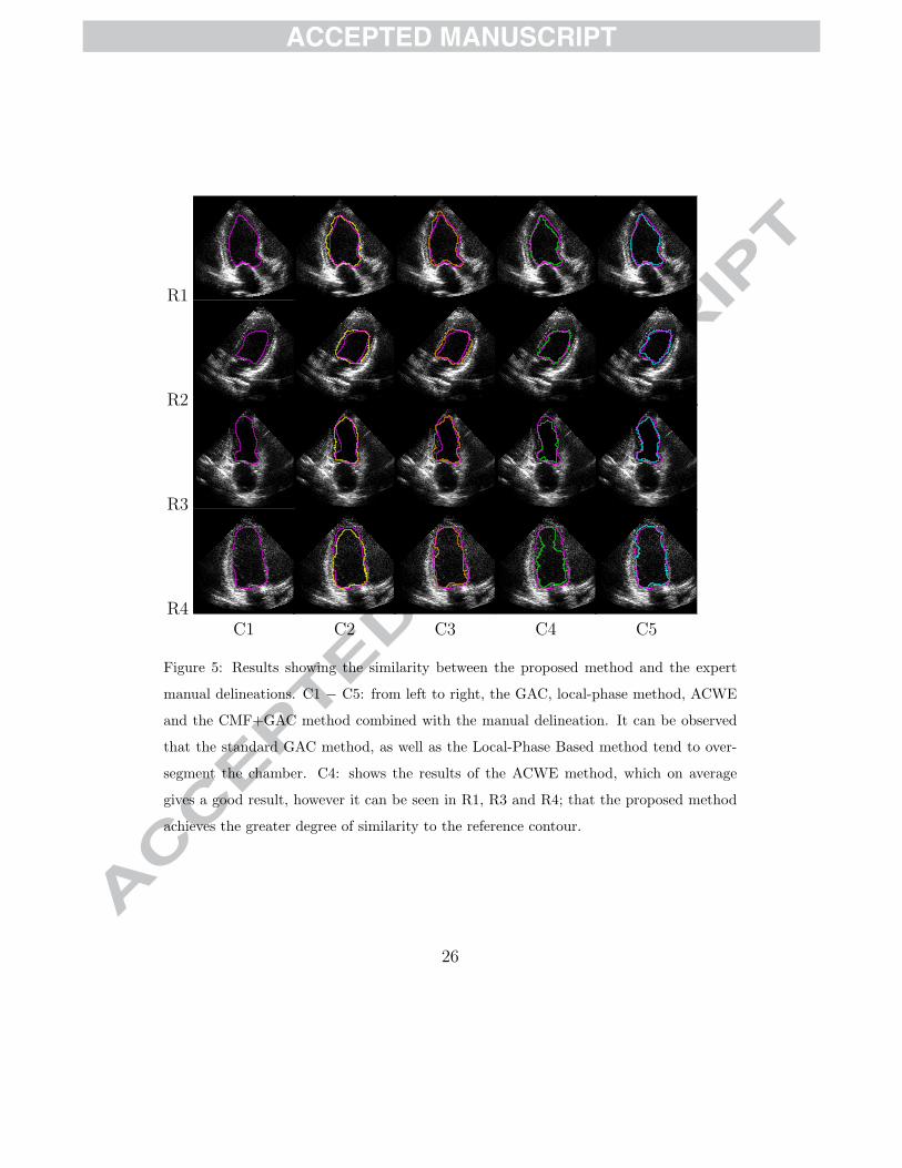
Qualitative results on the medical data are presented in Figures 4 and 5.254

Figure 4 shows the final result obtained with each method, while Figure 5255

shows the similarity of each method to the reference delineation.256

Starting with Row 1 in Figures 4 and 5, with respect to the GAC method,257

it can be seen (for example in Figure 4 (R1,C2)), that the absence of a sharp258

contrast in the upper right corner causes the method to over segment the259

chamber in this region. The local-phase based method performs compara-260

tively well, however over segments the chamber in the upper left region. The261

ACWE method produces a better result, however slightly under segments the262

chamber in this same region. The proposed CMF + GAC method achieves263

a result visually quite similar to the manual delineation.264

In Row 2 of Figures (4,5), the ACWE obtains the most accurate result265

(see Figure 5 (R2,C2)). The absence of a sharp boundary disrupts the GAC266

method while the local-phase method over segments the chamber. The pro-267

posed CMF + GAC method obtains a mostly accurate result, however under268

14

segments the chamber in the lower left region.269

Row 3 presents an example of an abnormally shaped chamber as well as270

limited window width in the upper right region. As in the previous examples,271

the GAC and local-phase based methods tend to over-segment (see Figures272

5 (R3,C2-C3) while the ACWE method, together with the CMF + GAC273

approach capture the true shape more accurately. The CMF + GAC method274

obtains a greater degree of similarity in the upper region of the chamber.275

The frame in Row 4 presents an example of the lack of intensity homo-276

geneity often found in echocardiographic data. The ACWE method (Figure277

4 (R4,C4) and Figure 5 (R4,C4)) finds the cleanest part of the chamber,278

however, as highlighted by the manual delineation, this does not represent279

the true boundary. The results obtained by both the local-phase as well as280

the CMF + GAC methods are visually quite similar, the phase based method281

achieves a smoother boundary. The GAC method slightly under-segments282

the upper chamber region.283

Figure 1 presents the results of testing the CMF + GAC method, together284

with the ACWE and GAC method on an image of a galaxy. The results show285

that the GAC method finds the strongest boundary therefore missing the286

lower gradient regions, while the ACWE method captures the bright star-287

like points dotted around the image, which are not part of the galaxy, it can288

be observed that the CMF + GAC results achieves the best approximation289

of the boundary.290

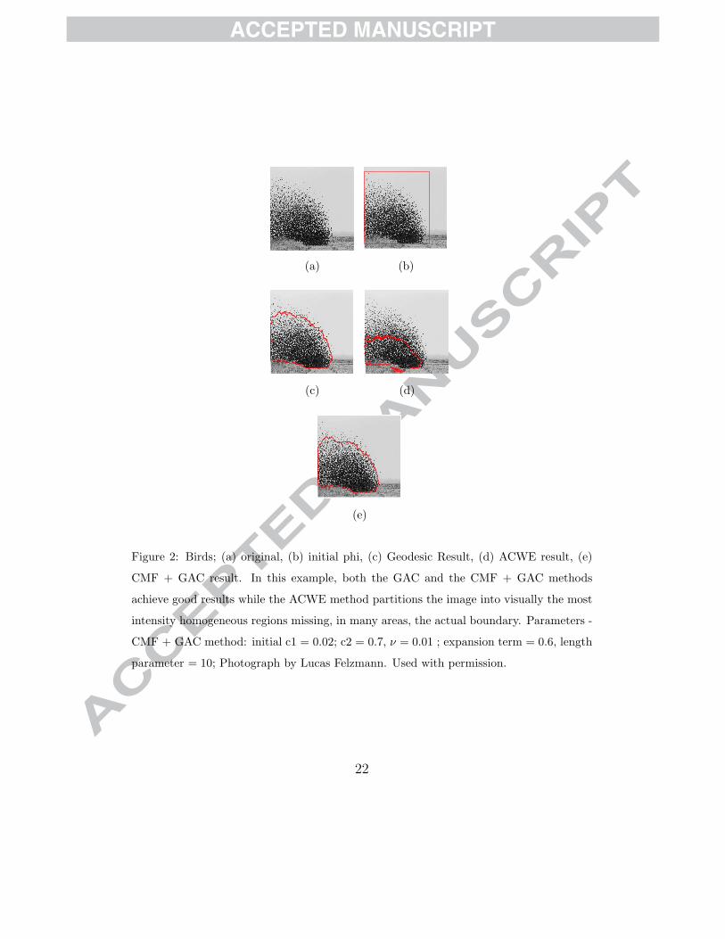
Figure 2 gives an example of birds swarming. In this example, the final291

results of both the GAC and the CMF + GAC methods, are quite simi-292

lar, both giving the approximate boundary of the swarm; while the ACWE293

15

method partitions the image into visually the most intensity homogeneous294

regions, consequently missing, in many areas, the actual boundary. Both the295

GAC and CMF + GAC methods achieve comparable results, with a smoother296

boundary than ACWE.297

Table 2 gives the average for all datasets of the percentage error due to298

change in the parameters used for each method. The CMF + GAC method299

shows robust performance with respect to the length parameter, however300

changing the initial estimates for inner and outer region intensity produces301

a significant fluctuation in performance, this is mirrored, though to a lesser302

degree, in the percentage error due to the image or contrast parameter in the303

ACWE methods. Among the details which are highlighted in this table is304

the lack of stability of the GAC method with this data; shifting the length305

parameter by 5% for example, produces an error of almost 44% in the final306

result.307

4. Discussion308

It can be observed from the results of the experiments on non-medical309

data, that the CMF + GAC approach achieves either similar performance310

to both the ACWE and GAC methods or enhanced performance in certain311

cases; for example due to the lack of sharp contrast as illustrated in Figure312

1, causing the GAC approach to fail, or when the predominant intensity313

densities do not represent the actual boundary as in Figure 2, which disrupts314

the ACWE method. The CMF + GAC approach achieves enhanced results315

compared to either method in these instances. The qualitative results for the316

medical data in Figures 4 to 5 largely mirror this observation.317

16

With respect to the quantitative results in Table 1, for each metric the318

proposed approach achieved the best overall result compared to each refer-319

ence method; achieving an average Hausdorff metric of 4.48mm, an average320

Mean Absolute Distance of 1.31mm and an average Dice coefficient of 0.91.321

Comparing these results to the next most accurate method, which was the322

GAC method, we see that for the Hausdorff metric, this represented a 5%323

improvement on the GAC method, a 40% improvement as measured by Mean324

Absolute Distance, while for the Dice coefficient, an improvement of 3% was325

gained. With respect to individual datasets, we can observe that in 4 out of326

5 cases the proposed approach achieved the lowest Hausdorff Distance, for327

the Mean Absolute Distance this was the case in 3 out of 5 cases, while again328

in 4 out 5 cases the proposed method achieved the best, or joint best result329

with respect to the Dice coefficient.330

The results also highlight some limitations of the model, such as in Figure331

5 (R2,C5). In this example, due to the extremely low contrast boundary in332

the left region of the chamber, the length parameter of the CMF method333

was strongly relaxed, which has the positive effect of reinforcing the bound-334

ary but also preserving noise (as exhibited in Figures 3(e),(f)). This effect335

disrupted the CMF + GAC approach in this instance. This result is also336

connected to the fluctuation in performance highlighted in sensitivity results337

in Table 2. Due to the lack of clear distinction between the intensity char-338

acteristics of the regions (i.e. the inner chamber and the inner wall of the339

myocardium), choosing data fidelity parameters which are robust with re-340

spect to variation is a challenging task. The sensitivity results in Table 2 for341

each of the CMF + GAC, ACWE and GAC approaches reflect this finding.342

17

These results highlight the limitations of data driven approaches in general,343

in handling particularly low quality data. Notwithstanding this observed344

fluctuation, however; and considering the results as a whole, it can be ob-345

served that the CMF + GAC approach gives the most robust response with346

respect to accuracy. Overall the sensitivity results indicate that the local-347

phase approach is the most robust with respect to parameter variance, while348

this approach achieved the least accuracy in terms of similarity to manual349

delineation.350

When considering the quantitative results in Table 1, it can be seen that351

using the level-set ACWE method on the whole, while less accurate than352

the CMF + GAC approach, is capable of achieving reasonable results on353

low quality data. With this in mind, it could be asked what advantage does354

solving the Mumford-Shah functional using the CMF approach have over a355

traditional level set formulation?356

In the traditional ACWE approach, tuning all algorithmic parameters357

can be a challenging and rather unintuitive process, for example it needs to358

be decided how often and accurately the level set function should be initial-359

ized, how the time step sizes should be chosen etc. Choosing the correct360

parameters for the CMF approach essentially means selecting the regulariza-361

tion parameter ν and the penalty parameter c in the Augmented Lagrangian362

method. The algorithm converges reliably for a wide range of c, (in all of363

our experiments, this value remained unchanged). In addition, the CMF ap-364

proach shows good robustness with respect to parameter ν (compare rows 2365

to 3) under CMF + GAC approach, to rows 2-3 of ACWE method, in Table366

2. The CMF approach is guaranteed to converge to a global minimizer, in367

18

contrast to the level set approach which may get stuck in an inferior local368

minimum.369

The combination of the CMF approach with the GAC method also has370

some interesting properties with respect to topology. Although the method371

contains no explicit topology preserving constraint, by relaxing the length372

constraint for the CMF approach, it becomes possible to favor the generation373

of closed regions, this is shown for example in Figure 3(e). Figure 4 (R1,C3),374

however, shows an example where this is impossible. In this example, the top375

left portion of the chamber is outside of the viewing window, as such there376

is not enough information for the CMF method to ‘reinforce’ the boundary,377

however, by increasing the stiffness properties of the GAC contour, it is still378

possible to maintain a closed topology. The reason for this is that the GAC379

method converges to a local minimizer with simple topology, which in this380

application is a better solution than the global minimizer. In this way the381

combination of local and global segmentation methods works to preserve382

topology.383

While it has been shown that the proposed method is capable of accu-384

rately segmenting low contrast images; it should be noted that the described385

method to generate edge sets (step 1) is not proposed as a general edge detec-386

tor approach, the detection of extremely fine structures, for example, would387

prove problematic for the model. Instead the method has been designed for388

the partition of structures with weak boundaries, as exemplified in a vari-389

ety of real-world applications, a sample of which we have highlighted in the390

current paper.391

Finally, when observing the results it can be seen that global features392

19

play a more significant role in the results achieved by the CMF + GAC393

method, than local edge features, this is a key aspect of the method. While394

the overall objective of the scheme is accurate boundary estimation, this goal395

is achieved by integrating regional information into the edge detector process396

using the CMF method, it is this regional information which makes boundary397

reinforcement possible.398

5. Conclusion399

In this work we have presented a method to generate edge detectors which400

allow for the effective segmentation of regions bounded by weak edges and401

have demonstrated its performance on a sample of real-world medical and402

non-medical data. It was shown that compared to classical image driven403

approaches, the proposed method is capable of more accurately detecting404

boundaries from low contrast images.405

The method we have proposed increases robustness in two ways - first by406

incorporating regional information into the process of edge map generation,407

weak boundaries are effectively reinforced, secondly the edge map output408

which corresponds to a 2 region global segmentation result, gives a more409

robust solution compared to traditional purely variational based schemes.410

Overall, we believe that both the qualitative and quantitative results411

clearly demonstrate the improved performance of the CMF + GAC approach412

over purely regional or intensity based methods as exemplified in the GAC413

and ACWE methods.414

20

(a)

(b) (c)

(d) (e)

Figure 1: Sombrero galaxy image [8]. The blue glow corresponds to the combined light

of billions of old stars and the orange ring marks the sites of young stars: (a) original

image, (b) initial phi,(c) Geodesic Result,(d) ACWE result, (e) CMF + GAC result. The

results show that the GAC method finds the strongest boundary therefore missing the

lower gradient regions (which also form part of the galaxy), while both the ACWE and

CMF + GAC methods achieve accurate results. Parameters used for the CMF + GAC

method: c1 = 0.18; c2 = 0.09; ν = 5e − 1, expansion term = 1, length parameter = 10.

Courtesy NASA/JPL-Caltech

21

(a) (b)

(c) (d)

(e)

Figure 2: Birds; (a) original, (b) initial phi, (c) Geodesic Result, (d) ACWE result, (e)

CMF + GAC result. In this example, both the GAC and the CMF + GAC methods

achieve good results while the ACWE method partitions the image into visually the most

intensity homogeneous regions missing, in many areas, the actual boundary. Parameters -

CMF + GAC method: initial c1 = 0.02; c2 = 0.7, ν = 0.01 ; expansion term = 0.6, length

parameter = 10; Photograph by Lucas Felzmann. Used with permission.

22

Table 1: Quantitative results computed using Hausdorff, Mean Absolute Distance and

Dice metrics for medical data. Experiments were conducted on a sample of 55 frames

across 5 datasets. Represented here is the average distance for each metric computed over

a test set of frames from each dataset

HD

LAX1 LAX2 LAX3 LAX4 LAX6 Average % diff

Our proposed Method 4.6 5.28 3.34 4.69 4.49 4.48

ACWE 6.78 9.91 3.37 5.91 5.47 6.29 40.4

Standard geodesic 5.31 3.8 4.08 5.64 4.66 4.7 4.9

Using Phase derived edge maps 6.62 5.48 5.02 8.22 8.52 6.77 51.1

MAD

LAX1 LAX2 LAX3 LAX4 LAX6 Average % diff

Our proposed Method 1.17 1.51 0.94 1.54 1.41 1.31

ACWE 1.82 3.46 0.89 1.9 1.45 1.9 45

Standard geodesic 2.06 1.39 1.81 1.85 2.11 1.84 40.5

Using Phase derived edge maps 1.72 1.6 1.98 2.26 1.95 1.9 45

Dice

LAX1 LAX2 LAX3 LAX4 LAX6 Average % diff

Our proposed Method 0.93 0.92 0.93 0.88 0.9 0.91

ACWE 0.87 0.75 0.93 0.84 0.9 0.86 5

Standard geodesic 0.89 0.93 0.87 0.87 0.86 0.88 3

Using Phase derived edge maps 0.9 0.9 0.85 0.83 0.87 0.87 4

23

(a) Original Image(b) Output of

CMF method

(c) Edge map

(d) Original Image(e) Output of

CMF method

(f) Edge map

(g) Output of

CMF method,

increased ν

(h) Corresponding

Edge map

Figure 3: Example output of CMF method for 2 datasets; (a) and (d) original frames; (b),

(e) and (g) corresponding output of CMF method, using values of ν = 0.5, ν = 1e − 02

and ν = 0.5 respectively; (c), (f) and (h) edge map generated from binary segmentation.

Figures (e) and (g) show the difference produced by varying ν,(g) shows a cleaner result

however (e) more accurately represents the underlying (closed) structure. The output of

the CMF method is only shown to illustrate each step of the proposed method and is not

part of the final output. To save space, the CMF result is only shown for a subset of the

experiments.

24

R1

R2

R3

R4C1 C2 C3 C4 C5

Figure 4: Results achieved by each method on four sample frames (Rows R1 R4). Each

frame shows an example of boundaries characterized by weak edges. C1: The original

frame. C2: Standard GAC method. C3: Local-phase based method. C4: ACWE method.

C5: Results obtained using the proposed method.

25

R1

R2

R3

R4

C1 C2 C3 C4 C5

Figure 5: Results showing the similarity between the proposed method and the expert

manual delineations. C1 − C5: from left to right, the GAC, local-phase method, ACWE

and the CMF+GAC method combined with the manual delineation. It can be observed

that the standard GAC method, as well as the Local-Phase Based method tend to over-

segment the chamber. C4: shows the results of the ACWE method, which on average

gives a good result, however it can be seen in R1, R3 and R4; that the proposed method

achieves the greater degree of similarity to the reference contour.

26

Table 2: Percentage error due to each parameter. Average taken over all frames

Proposed Method HD MAD Dice

Average Std Average Std Average Std

vary length parameter by +/- 5% 0.92 1.12 0.16 0.15 0.01 0.01

vary length parameter by +/- 10% 1.74 1.94 0.38 0.37 0.03 0.03

vary length parameter by +/- 20% 6.33 11.57 2.68 5.83 0.26 0.61

vary c1 or c2 by +/- 5% 5.59 9.47 3.36 4.48 0.93 1.35

vary c1 or c2 by +/- 10% 12.12 22.97 6.41 8.99 1.34 1.75

vary c1 or c2 by +/- 20% 28.71 44.09 13.64 16.51 2.37 2.48

Expansion Parameter (tuned for 1 dataset)

vary expansion parameter by +/-5% 6.39 6.39 2.99 1.51 0.41 0

vary expansion parameter by +/-10% 14.5 1.72 12.13 10.65 1.32 0.91

vary expansion parameter by +/-20% 74.69 60.21 28.28 25.74 5.99 5.5

ACWE HD MAD Dice

Average Std Average Std Average Std

vary length parameter by +/-5% 4.19 9.38 3.12 6.02 1.12 2.96

vary length parameter by +/-10% 11.71 19.02 5.55 6.47 1.52 2.3

vary length parameter by +/-20% 11.03 8.48 6.12 4.76 1.59 2.23

vary image parameter by +/-5% 15.96 20.53 7.09 8.64 1.95 3.18

vary image parameter by +/-10% 20.15 28.63 7.62 8.55 2.06 2.86

vary image parameter by +/-20% 31.57 33.87 16.6 15.49 3.86 4.08

GAC HD MAD Dice

Average Std Average Std Average Std

vary expansion parameter by +/-5% 25.64 36.9 21.09 30.5 4.68 7.69

vary expansion parameter by +/-10% 48.92 35.57 47.1 28.44 10.37 7.86

vary expansion parameter by +/-20% 102.89 56.99 87.07 50.38 13.98 10.32

vary contour parameter by +/-5% 43.78 61.76 34.42 44.15 6.49 7.21

vary contour parameter by +/-10% 44.48 61.26 35.53 43.12 5.54 7.07

vary contour parameter by +/-20% 47.74 60.45 38.8 40.23 6.39 6.58

Phase HD MAD Dice

Average Std Average Std Average Std

vary wavelength parameter by +/-5% 6.63 5.06 2.55 1.75 0.41 0.37

vary wavelength parameter by +/-10% 7.5 5.25 3.9 2.51 0.68 0.55

vary wavelength parameter by +/-20% 10.31 5.28 5.95 3.03 0.91 0.59

Expansion Parameter (tuned for 3 datasets)

vary expansion parameter by +/-5% 0 0 0.01 0.01 0 0

vary expansion parameter by +/-10% 2.18 2.36 1.24 1.12 0.23 0.2

vary expansion parameter by +/-20% 11.74 10.81 6.85 4.42 1.27 0.87

27

Acknowledgements415

The authors would especially like to thank the authors of [19] for pro-416

viding us with the implementation of the Local Phase method as well as417

the anonymous reviewers for their valuable comments and suggestions. This418

work was supported by the National Science Foundation grant NSF DMS-419

1217239, UC Lab Fees Research grant 12-LR-23660, Norwegian Research420

Council eVita project 214889 and the Irish Research Council.421

References422

[1] Bresson, X., Esedoglu, S., Vandergheynst, P., Thiran, J.P., Osher, S.,423

2007. Fast global minimization of the active contour/snake model. J424

Math Imaging Vis 28, 151–167.425

[2] Bui, T.D., Gao, S., Zhang, Q., 2005. A generalized mumford-shah model426

for roof-edge detection, in: ICIP (2), pp. 1214–1217.427

[3] Caselles, V., Kimmel, R., Sapiro, G., 1997. Geodesic active contours.428

Int J Comput Vision 22, 61–79.429

[4] Chan, T., Esedoglu, S., Nikolova, M., 2006. Algorithms for finding global430

minimizers of image segmentation and denoising models. Siam J Appl431

Math , 17 pp.432

[5] Chan, T., Vese, L., 2001. Active contours without edges. IEEE T Image433

Process 10, 266–277.434

[6] Duggan, N., Schaeffer, H., Guyader, C.L., Jones, E., Glavin, M., Vese,435

L., 2013. Boundary detection in echocardiography using a split bregman436

28

edge detector and a topology-preserving level set approach, in: Interna-437

tional Symposium on Biomedical Imaging (ISBI), IEEE.438

[7] Felsberg, M., Sommer, G., 2001. The monogenic signal. IEEE Transac-439

tions on Signal Processing 49, 3136–3144.440

[8] Ford, H.C., Hui, X., Ciardullo, R., Jacoby, G.H., Freeman, K.C., 1996.441

The stellar halo of M104. I. A survey for planetary nebulae and the442

planetary nebula luminosity function distance. Astrophysical Journal443

458, 455–466. doi:doi:10.1086/176828.444

[9] Goldstein, T., Bresson, X., Osher, S., 2010. Geometric applications of445

the split bregman method: Segmentation and surface reconstruction. J.446

Sci. Comput. 45, 272–293.447

[10] Hyman, J.M., Shashkov, M.J., 1997. Natural discretizations for the448

divergence, gradient, and curl on logically rectangular grids. Comput.449

Math. Appl. 33, 81–104.450

[11] Kass, M., Witkin, A., Terzopoulos, D., 1987. Snakes: Active contour451

models. Int J Comput Vision , 321 –331.452

[12] Kichenassamy, S., Kumar, A., Olver, P., Tannenbaum, A., Yezzi, A.,453

1996. Conformal curvature flows: from phase transitions to active vision.454

Arch. Rat. Mech. Anal. 134, 275–301.455

[13] Mulet-Parada, M., Noble, J., 2000. 2d+t acoustic boundary detection456

in echocardiography. Medical Image Analyis 4, 21–30.457

29

[14] Mumford, D., Shah, J., 1989. Optimal approximations by458

piecewise smooth functions and associated variational problems.459

Communications on Pure and Applied Mathematics 42, 577–685.460

doi:10.1002/cpa.3160420503.461

[15] Osher, S., Sethian, J.A., 1988. Fronts propagating with curvature-462

dependent speed: algorithms based on hamilton-jacobi formulations. J463

Comput Phys 79, 12–49.464

[16] Paragios, N., Deriche, R., 1999. Unifying boundary and region-based465

information for geodesic active tracking, in: IEEE Conference on Com-466

puter Vision and Pattern Recognition.467

[17] Perona, P., Malik, J., 1990. Scale-space and edge detection using468

anisotropic diffusion. IEEE Trans. Pattern Anal. Mach. Intell. 12, 629–469

639.470

[18] Pock, T., Cremers, D., Bischof, H., Chambolle, A., 2009. An algorithm471

for minimizing the mumford-shah functional, in: ICCV, pp. 1133–1140.472

[19] Rajpoot, K., Grau, V., Noble, J., 2009a. Local-phase based 3d bound-473

ary detection using monogenic signal and its application to real-time474

3-d echocardiography images, in: IEEE International Symposium on475

Biomedical Imaging, pp. 783 –786.476

[20] Rajpoot, K., Noble, J.A., Grau, V., Szmigielski, C., Becher, H., 2009b.477

Image-driven cardiac left ventricle segmentation for the evaluation of478

multiview fused real-time 3-dimensional echocardiography images, in:479

MICCAI, pp. 893–900.480

30

[21] Schaeffer, H., 2012. Active arcs and contours. UCLA CAM Report 12-481

54. URL: ftp://ftp.math.ucla.edu/pub/camreport/cam12-54.pdf.482

[22] Schaeffer, H., Vese, L., 2013. Active contours with free endpoints. Jour-483

nal of Mathematical Imaging and Vision , 1–17.484

[23] Vese, L., Chan, T., 2002. A multiphase level set framework for image485

segmentation using the mumford and shah model. Int J Comput Vision486

50, 271–293.487

[24] Wang, L.L., Shi, Y., Tai, X.C., 2012. Robust edge detection using488

mumford-shah model and binary level set method, in: Bruckstein, A.,489

Haar Romeny, B., Bronstein, A., Bronstein, M. (Eds.), Scale Space and490

Variational Methods in Computer Vision. volume 6667 of LNCS, pp.491

291–301.492

[25] Weickert, J., Romeny, B.M.T.H., Viergever, M.A., 1998. Efficient and493

reliable schemes for nonlinear diffusion filtering. IEEE Transactions on494

Image Processing 7, 398–410.495

[26] Yuan, J., Bae, E., Tai, X.C., 2010. A study on continuous max-flow496

and min-cut approaches, in: Computer Vision and Pattern Recognition497

(CVPR), 2010 IEEE Conference on, pp. 2217–2224.498

[27] Yuan, J., Bae, E., Tai, X.C., Boykov, Y., 2014. A spatially continuous499

max-flow and min-cut framework for binary labeling problems. Nu-500

merische Mathematik 126, 559–587.501

31

Highlights:

An method for segmentation of low contrast images is proposed

The global optimal output of the CV model is used to create the edge attraction force in the GAC method.

Experimental results demonstrate improved performance over existing data driven methods