A Simple and Effective Model-BasedVariable Importance Measure

Brandon M. Greenwell ∗

Wright State Universityand

Bradley C. BoehmkeUniversity of Cincinnati

andAndrew J. McCarthyThe Perduco Group

May 15, 2018

Abstract

In the era of “big data”, it is becoming more of a challenge to not only buildstate-of-the-art predictive models, but also gain an understanding of what’s reallygoing on in the data. For example, it is often of interest to know which, if any, of thepredictors in a fitted model are relatively influential on the predicted outcome. Somemodern algorithms—like random forests and gradient boosted decision trees—have anatural way of quantifying the importance or relative influence of each feature. Otheralgorithms—like naive Bayes classifiers and support vector machines—are not capableof doing so and model-free approaches are generally used to measure each predictor’simportance. In this paper, we propose a standardized, model-based approach tomeasuring predictor importance across the growing spectrum of supervised learningalgorithms. Our proposed method is illustrated through both simulated and real dataexamples. The R code to reproduce all of the figures in this paper is available in thesupplementary materials.

Keywords: Relative influence, Interaction effect, Partial dependence function, Partial de-pendence plot, PDP

∗The authors gratefully acknowledge . . .

1

arX

iv:1

805.

0475

5v1

[st

at.M

L]

12

May

201

8

1 Introduction

Complex supervised learning algorithms, such as neural networks (NNs) and support vec-

tor machines (SVMs), are more common than ever in predictive analytics, especially when

dealing with large observational databases that don’t adhere to the strict assumptions im-

posed by traditional statistical techniques (e.g., multiple linear regression which typically

assumes linearity, homoscedasticity, and normality). However, it can be challenging to

understand the results of such complex models and explain them to management. Graph-

ical displays such as variable importance plots (when available) and partial dependence

plots (PDPs) (Friedman 2001) offer a simple solution (see, for example, Hastie et al. 2009,

pp. 367–380). PDPs are low-dimensional graphical renderings of the prediction function

f (x) that allow analysts to more easily understand the estimated relationship between the

outcome and predictors of interest. These plots are especially useful in interpreting the

output from “black box” models. While PDPs can be constructed for any predictor in a

fitted model, variable importance scores are more difficult to define, and when available,

their interpretation often depends on the model fitting algorithm used.

In this paper, we consider a standardized method to computing variable importance

scores using PDPs. There are a number of advantages to using our approach. First,

it offers a standardized procedure to quantifying variable importance across the growing

spectrum of supervised learning algorithms. For example, while popular statistical learn-

ing algorithms like random forests (RFs) and gradient boosted decision trees (GBMs) have

there own natural way of measuring variable importance, each is interpreted differently

(these are briefly described in Section 2.1). Secondly, our method is suitable for use with

any trained supervised learning algorithm, provided predictions on new data can be ob-

tained. For example, it is often beneficial (from an accuracy standpoint) to train and tune

multiple state-of-the art predictive models (e.g., multiple RFs, GBMs, and deep learning

NNs (DNNs)) and then combine them into an ensemble called a super learner through a

process called model stacking. Even if the base learners can provide there own measures of

variable importance, there is no logical way to combine them to form an overall score for

the super learner. However, since new predictions can be obtained from the super learner,

our proposed variable importance measure is still applicable (examples are given in Sec-

2

tions 5–6). Thirdly, as shown in Section 3.2, our proposed method can be modified to

quantify the strength of potential interaction effects. Finally, since our approach is based

on constructing PDPs for all the main effects, the analyst is forced to also look at the

estimated functional relationship between each feature and the target—which should be

done in tandem with studying the importance of each feature.

2 Background

We are often confronted with the task of extracting knowledge from large databases. For

this task we turn to various statistical learning algorithms which, when tuned correctly,

can have state-of-the-art predictive performance. However, having a model that predicts

well is only solving part of the problem. It is also desirable to extract information about

the relationships uncovered by the learning algorithm. For instance, we often want to know

which predictors, if any, are important by assigning some type of variable importance score

to each feature. Once a set of influential features has been identified, the next step is

summarizing the functional relationship between each feature, or subset thereof, and the

outcome of interest. However, since most statistical learning algorithms are “black box”

models, extracting this information is not always straightforward. Luckily, some learning

algorithms have a natural way of defining variable importance.

2.1 Model-based approaches to variable importance

Decision trees probably offer the most natural model-based approach to quantifying the

importance of each feature. In a binary decision tree, at each node t, a single predictor

is used to partition the data into two homogeneous groups. The chosen predictor is the

one that maximizes some measure of improvement it. The relative importance of predictor

x is the sum of the squared improvements over all internal nodes of the tree for which

x was chosen as the partitioning variable; see Breiman et al. (1984) for details. This

idea also extends to ensembles of decision trees, such as RFs and GBMs. In ensembles,

the improvement score for each predictor is averaged across all the trees in the ensemble.

Fortunately, due to the stabilizing effect of averaging, the improvement-based variable

3

importance metric is often more reliable in large ensembles (see Hastie et al. 2009, pg.

368). RFs offer an additional method for computing variable importance scores. The idea

is to use the leftover out-of-bag (OOB) data to construct validation-set errors for each tree.

Then, each predictor is randomly shuffled in the OOB data and the error is computed

again. The idea is that if variable x is important, then the validation error will go up when

x is perturbed in the OOB data. The difference in the two errors is recorded for the OOB

data then averaged across all trees in the forest.

In multiple linear regression, the absolute value of the t-statistic is commonly used as

a measure of variable importance. The same idea also extends to generalized linear mod-

els (GLMs). Multivariate adaptive regression splines (MARS), which were introduced in

Friedman (1991a), is an automatic regression technique which can be seen as a generaliza-

tion of multiple linear regression and generalized linear models. In the MARS algorithm,

the contribution (or variable importance score) for each predictor is determined using a

generalized cross-validation (GCV) statistic.

For NNs, two popular methods for constructing variable importance scores are the

Garson algorithm (Garson 1991), later modified by Goh (1995), and the Olden algorithm

(Olden et al. 2004). For both algorithms, the basis of these importance scores is the

network’s connection weights. The Garson algorithm determines variable importance by

identifying all weighted connections between the nodes of interest. Olden’s algorithm, on

the other hand, uses the product of the raw connection weights between each input and

output neuron and sums the product across all hidden neurons. This has been shown to

outperform the Garson method in various simulations. For DNNs, a similar method due to

Gedeon (1997) considers the weights connecting the input features to the first two hidden

layers (for simplicity and speed); but this method can be slow for large networks.

2.2 Filter-based approaches to variable importance

Filter-based approaches, which are described in Kuhn & Johnson (2013), do not make use

of the fitted model to measure variable importance. They also do not take into account

the other predictors in the model.

For regression problems, a popular approach to measuring the variable importance of a

4

numeric predictor x is to first fit a flexible nonparametric model between x and the target Y ;

for example, the locally-weighted polynomial regression (LOWESS) method developed by

Cleveland (1979). From this fit, a pseudo-R2 measure can be obtained from the resulting

residuals and used as a measure of variable importance. For categorical predictors, a

different method based on standard statistical tests (e.g., t-tests and ANOVAs) is employed;

see Kuhn & Johnson (2013) for details.

For classification problems, an area under the ROC curve (AUC) statistic can be used

to quantify predictor importance. The AUC statistic is computed by using the predictor

x as input to the ROC curve. If x can reasonably separate the classes of Y , that is a

clear indicator that x is an important predictor (in terms of class separation) and this is

captured in the corresponding AUC statistic. For problems with more than two classes,

extensions of the ROC curve or a one-vs-all approach can be used.

2.3 Partial dependence plots

Harrison & Rubinfeld (1978) analyzed a data set containing suburban Boston housing

data from the 1970 census. They sought a housing value equation using an assortment of

features; see Table IV of Harrison & Rubinfeld (1978) for a description of each variable.

The usual regression assumptions, such as normality, linearity, and constant variance, were

clearly violated, but through an exhausting series of transformations, significance testing,

and grid searches, they were able to build a model which fit the data reasonably well

(R2 = 0.81). Their prediction equation is given in Equation (1). This equation makes

interpreting the model easier. For example, the average number of rooms per dwelling

(RM) is included in the model as a quadratic term with a positive coefficient. This means

that there is a monotonic increasing relationship between RM and the predicted median

home value, but larger values of RM have a greater impact.

5

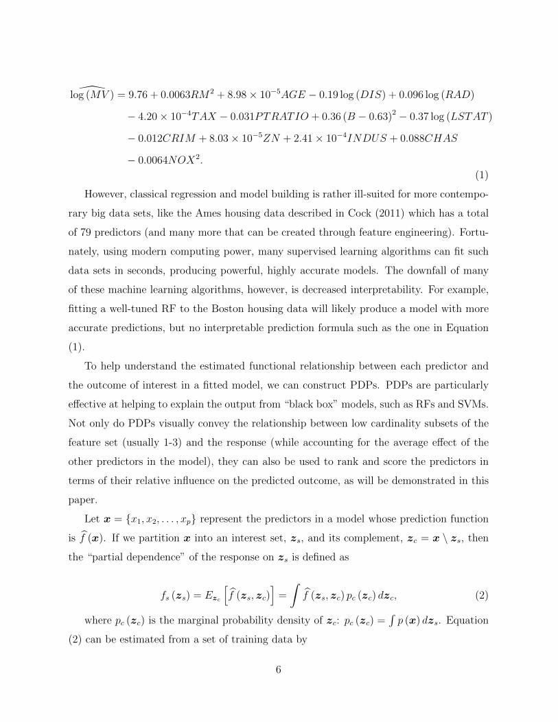
log (MV ) = 9.76 + 0.0063RM2 + 8.98× 10−5AGE − 0.19 log (DIS) + 0.096 log (RAD)

− 4.20× 10−4TAX − 0.031PTRATIO + 0.36 (B − 0.63)2 − 0.37 log (LSTAT )

− 0.012CRIM + 8.03× 10−5ZN + 2.41× 10−4INDUS + 0.088CHAS

− 0.0064NOX2.

(1)

However, classical regression and model building is rather ill-suited for more contempo-

rary big data sets, like the Ames housing data described in Cock (2011) which has a total

of 79 predictors (and many more that can be created through feature engineering). Fortu-

nately, using modern computing power, many supervised learning algorithms can fit such

data sets in seconds, producing powerful, highly accurate models. The downfall of many

of these machine learning algorithms, however, is decreased interpretability. For example,

fitting a well-tuned RF to the Boston housing data will likely produce a model with more

accurate predictions, but no interpretable prediction formula such as the one in Equation

(1).

To help understand the estimated functional relationship between each predictor and

the outcome of interest in a fitted model, we can construct PDPs. PDPs are particularly

effective at helping to explain the output from “black box” models, such as RFs and SVMs.

Not only do PDPs visually convey the relationship between low cardinality subsets of the

feature set (usually 1-3) and the response (while accounting for the average effect of the

other predictors in the model), they can also be used to rank and score the predictors in

terms of their relative influence on the predicted outcome, as will be demonstrated in this

paper.

Let x = {x1, x2, . . . , xp} represent the predictors in a model whose prediction function

is f (x). If we partition x into an interest set, zs, and its complement, zc = x \ zs, then

the “partial dependence” of the response on zs is defined as

fs (zs) = Ezc

[f (zs, zc)

]=

∫f (zs, zc) pc (zc) dzc, (2)

where pc (zc) is the marginal probability density of zc: pc (zc) =∫p (x) dzs. Equation

(2) can be estimated from a set of training data by

6

fs (zs) =1

n

n∑i=1

f (zs, zi,c) , (3)

where zi,c (i = 1, 2, . . . , n) are the values of zc that occur in the training sample; that

is, we average out the effects of all the other predictors in the model.

Constructing a PDP (3) in practice is rather straightforward. To simplify, let zs = x1

be the predictor variable of interest with unique values {x11, x12, . . . , x1k}. The partial

dependence of the response on x1 can be constructed as follows:

Input: the unique predictor values x11, x12, . . . , x1k;

Output: the estimated partial dependence values f1 (x11) , f1 (x12) , . . . , f1 (x1k).

for i ∈ {1, 2, . . . , k} do

(1) copy the training data and replace the original values of x1 with the constant

x1i;

(2) compute the vector of predicted values from the modified copy of the training

data;

(3) compute the average prediction to obtain f1 (x1i).

end

The PDP for x1 is obtained by plotting the pairs{x1i, f1 (x1i)

}for i = 1, 2, . . . , k.

Algorithm 1: A simple algorithm for constructing the partial dependence of the response

on a single predictor x1.

Algorithm 1 can be computationally expensive since it involves k passes over the train-

ing records. Fortunately, it is embarrassingly parallel and computing partial dependence

functions for each predictor can be done rather quickly on a machine with a multi-core

processor. For large data sets, it may be worthwhile to reduce the grid size by using

specific quantiles for each predictor, rather than all the unique values. For example, the

partial dependence function can be approximated very quickly by using the deciles of the

unique predictor values. The exception is classification and regression trees based on single-

variable splits which can make use of the efficient weighted tree traversal method described

in Friedman (2001).

7

While PDPs are an invaluable tool in understanding the relationships uncovered by

complex nonparametric models, they can be misleading in the presence of substantial in-

teraction effects (Goldstein et al. 2015). To overcome this issue, Goldstein et al. introduced

the concept of individual conditional expectation (ICE) curves. ICE curves display the es-

timated relationship between the response and a predictor of interest for each observation;

in other words, skipping step 1 (c) in Algorithm 1. Consequently, the PDP for a predictor

of interest can be obtained by averaging the corresponding ICE curves across all observa-

tions. Although ICE curves provide a refinement over traditional PDPs in the presence

of substantial interaction effects, in Section 3.2, we show how to use partial dependence

functions to evaluate the strength of potential interaction effects.

2.4 The Ames housing data set

For illustration, we will use the Ames housing data set—a modernized and expanded version

of the often cited Boston Housing data set. These data are available in the AmesHousing

package (Kuhn 2017). Using the R package h2o (The H2O.ai team 2017), we trained and

tuned a GBM using 10-fold cross-validation. The model fit is reasonable, with a cross-

validated (pseudo) R2 of 91.54%. Like other tree-based ensembles, GBMs have a natural

way of defining variable importance which was described in Section 2.1. The variable impor-

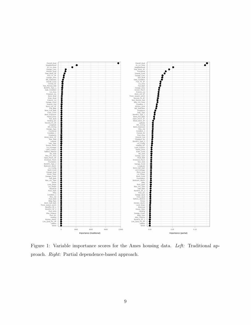
tance scores for these data are displayed in the left side of Figure 1. This plot indicates that

the overall quality of the material and finish of the house (Overall Qual), physical loca-

tion within the Ames city limits (Neighborhood), and the above grade (ground) living area

(Gr Liv Area) are highly associated with the logarithm of the sales price (Log Sale Price).

The variable importance scores also indicate that pool quality (Pool QC), the number of

kitchens above grade (Kitchen AbvGr), and the low quality finished square feet for all floors

(Low Qual Fin SF) have little association with Log Sale Price. (Note that the bottom two

features in Figure 1—Street and Utilities—have a variable importance score of exactly

zero; in other words, they were never used to partion the data at any point in the GBM

ensemble.)

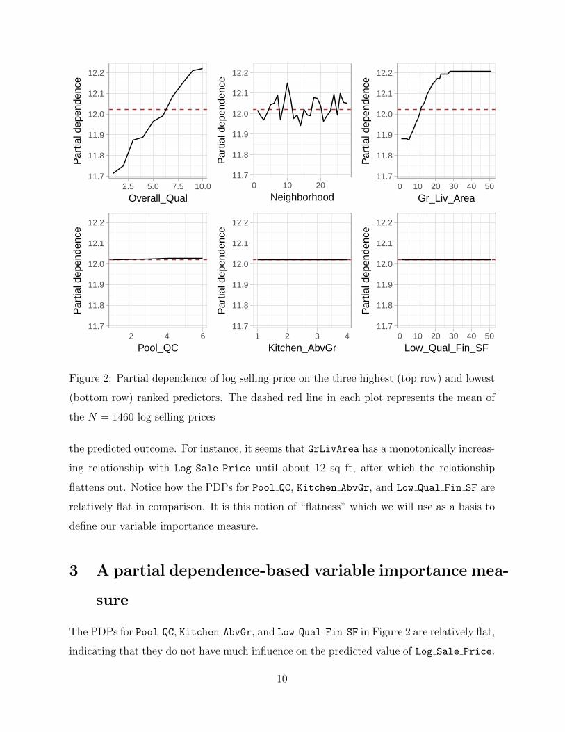
The PDPs for these six variables are displayed in Figure 2. These plots indicate that

Overall Qual, Neighborhood, and Gr Liv Area have a strong nonlinear relationship with

8

StreetUtilities

Low_Qual_Fin_SFKitchen_AbvGr

HeatingPool_QC

Misc_FeaturePool_Area

BsmtFin_SF_2BsmtFin_SF_1

Three_season_porchBsmt_Half_Bath

Bldg_TypeRoof_Matl

Misc_ValCondition_2

AlleyRoof_Style

ElectricalLot_Shape

Land_SlopeFence

Mas_Vnr_TypeHalf_Bath

Garage_FinishHouse_Style

Garage_QualBsmt_CondLot_Config

Bedroom_AbvGrBsmtFin_Type_2

FoundationEnclosed_PorchOpen_Porch_SF

Mas_Vnr_AreaMo_Sold

TotRms_AbvGrdLand_ContourLot_Frontage

Screen_PorchSale_Type

LatitudeYear_Sold

Wood_Deck_SFFireplaces

Condition_1Functional

Garage_TypeMS_Zoning

LongitudeSecond_Flr_SF

Heating_QCYear_Built

Paved_DriveBsmt_Exposure

Exter_CondBsmt_Full_Bath

Full_BathBsmt_Unf_SFExterior_2nd

Garage_CondExterior_1stExter_QualBsmt_Qual

Fireplace_QuLot_Area

Sale_ConditionBsmtFin_Type_1

Year_Remod_AddCentral_Air

Overall_CondMS_SubClassGarage_AreaFirst_Flr_SF

Total_Bsmt_SFKitchen_QualGarage_CarsGr_Liv_Area

NeighborhoodOverall_Qual

0 3000 6000 9000 12000

Importance (traditional)

StreetUtilities

Low_Qual_Fin_SFBsmtFin_SF_1

Misc_FeatureBldg_Type

Garage_FinishHeating

House_StyleElectrical

Land_SlopeKitchen_AbvGr

FenceTotRms_AbvGrd

Exter_QualGarage_Qual

Pool_QCBsmtFin_SF_2

Half_BathMas_Vnr_Type

Roof_StyleAlley

Bedroom_AbvGrFoundationBsmt_CondLot_ShapeBsmt_Qual

Lot_FrontageBsmt_Half_Bath

LongitudeGarage_Cond

Year_SoldEnclosed_Porch

Roof_MatlGarage_Type

Mo_SoldExter_Cond

Paved_DriveLand_Contour

Heating_QCLot_Config

BsmtFin_Type_2Fireplace_QuExterior_2nd

Pool_AreaCentral_Air

Condition_2Misc_Val

Bsmt_ExposureMS_Zoning

LatitudeWood_Deck_SFOpen_Porch_SFBsmt_Full_Bath

BsmtFin_Type_1Sale_TypeFireplaces

MS_SubClassKitchen_Qual

Condition_1Mas_Vnr_Area

Year_Remod_AddSecond_Flr_SF

Three_season_porchBsmt_Unf_SF

Exterior_1stScreen_PorchGarage_Area

Full_BathLot_Area

First_Flr_SFSale_Condition

Year_BuiltGarage_CarsOverall_Cond

FunctionalTotal_Bsmt_SFNeighborhood

Gr_Liv_AreaOverall_Qual

0.00 0.05 0.10

Importance (partial)

Figure 1: Variable importance scores for the Ames housing data. Left: Traditional ap-

proach. Right: Partial dependence-based approach.

9

11.7

11.8

11.9

12.0

12.1

12.2

2.5 5.0 7.5 10.0

Overall_Qual

Par

tial d

epen

denc

e

11.7

11.8

11.9

12.0

12.1

12.2

0 10 20

Neighborhood

Par

tial d

epen

denc

e

11.7

11.8

11.9

12.0

12.1

12.2

0 10 20 30 40 50

Gr_Liv_Area

Par

tial d

epen

denc

e

11.7

11.8

11.9

12.0

12.1

12.2

2 4 6

Pool_QC

Par

tial d

epen

denc

e

11.7

11.8

11.9

12.0

12.1

12.2

1 2 3 4

Kitchen_AbvGr

Par

tial d

epen

denc

e

11.7

11.8

11.9

12.0

12.1

12.2

0 10 20 30 40 50

Low_Qual_Fin_SF

Par

tial d

epen

denc

eFigure 2: Partial dependence of log selling price on the three highest (top row) and lowest

(bottom row) ranked predictors. The dashed red line in each plot represents the mean of

the N = 1460 log selling prices

the predicted outcome. For instance, it seems that GrLivArea has a monotonically increas-

ing relationship with Log Sale Price until about 12 sq ft, after which the relationship

flattens out. Notice how the PDPs for Pool QC, Kitchen AbvGr, and Low Qual Fin SF are

relatively flat in comparison. It is this notion of “flatness” which we will use as a basis to

define our variable importance measure.

3 A partial dependence-based variable importance mea-

sure

The PDPs for Pool QC, Kitchen AbvGr, and Low Qual Fin SF in Figure 2 are relatively flat,

indicating that they do not have much influence on the predicted value of Log Sale Price.

10

In other words, the partial dependence values fi (xij) (j = 1, 2, . . . , ki) display little vari-

ability. One might conclude that any variable for which the PDP is “flat” is likely to be less

important than those predictors whose PDP varies across a wider range of the response.

Our notion of variable importance is based on any measure of the “flatness” of the

partial dependence function. In general, we define

i (x) = z(fs (zs)

),

where z (·) is any measure of the “flatness” of fs (zs). A simple and effective measure

to use is the sample standard deviation for continuous predictors and the range statistic

divided by four for factors with K levels; the range divided by four provides an estimate

of the standard deviation for small to moderate sample sizes. Based on Algorithm 1, our

importance measure for predictor x1 is simply

i (x1) =

√

1k−1∑k

i=1

[f1 (x1i)− 1

k

∑ki=1 f1 (x1i)

]2if x1 is continuous[

maxi

(f1 (x1i)

)−mini

(f1 (x1i)

)]/4 if x1 is categorical

. (4)

Note that our variable importance metric relies on the fitted model; hence, it is crucial

to properly tune and train the model to attain the best performance possible.

To illustrate, we applied Algorithm 1 to all of the predictors in the Ames GBM model

and computed (4). The results are displayed in right side of Figure 1. In this case, our

partial dependence-based algorithm matches closely with the results from the GBM. In

particular, Figure ?? indicates that Overall Qual, Neighborhood, and Gr Liv Area are

still the most important variables in predicting Log Sale Price; though, Neighborhood

and Gr Liv Area have swapped places.

3.1 Linear models

As mentioned earlier, a natural choice for measuring the importance of each term in a linear

model is to use the absolute value of the corresponding coefficient divided by its estimated

standard error (i.e., the absolute value of the t-statistic). This turns out to be equivalent

to the partial dependence-based metric (4) when the predictors are independently and

uniformly distributed over the same range.

11

For example, suppose we have a linear model of the form

Y = β0 + β1X1 + β2X2 + ε,

where βi (i = 1, 2) is a constant, X1 and X2 are both independent U (0, 1) random

variables, and ε ∼ N (0, σ2). Since we know the distribution of X1 and X2, we can easily

find f1 (X1) and f2 (X2). For instance,

f1 (X1) =

∫ 1

0

E [Y |X1, X2] p (X2) dX2,

where p (X2) = 1. Simple calculus then leads to

f1 (X1) = β0 + β2/2 + β1X1 and f2 (X2) = β0 + β1/2 + β2X2..

Because E [Y |X1, X2] = f (X1, X2) is additive, the true partial dependence functions

are just simple linear regressions in each predictor with their original coefficient and an

adjusted intercept. Taking the variance of each gives

V ar [f1 (X1)] = β21/12 and V ar [f2 (X2)] = β2

2/12.

Hence, the standard deviations are just the absolute values of the original coefficients

(scaled by the same constant).

To illustrate, we simulated n = 1000 observations from the following linear model

Y = 1 + 3X1 − 5X2 + ε,

where X1 and X2 are both independent U (0, 1) random variables, and ε ∼ N (0, 0.012).

For this example, we have

f1 (X1) = −3

2+ 3X1 and f2 (X1) =

5

2− 5X2.

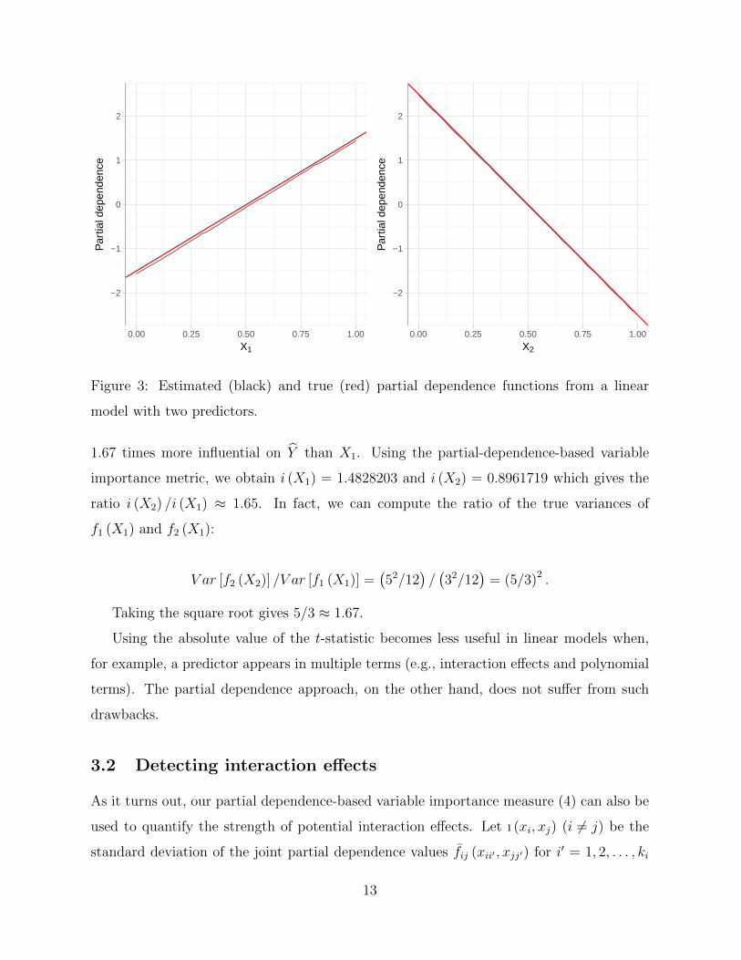
These are plotted as red lines in Figure 3. Additionally, the black lines in Figure 3

correspond to the estimated partial dependence functions using Algorithm 1.

Based on these plots, X2 is more influential than X1. Taking the absolute value of the

ratio of the slopes in f2 (X2) and f1 (X1) gives 5/3 ≈ 1.67. In other words, X2 is roughly

12

−2

−1

0

1

2

0.00 0.25 0.50 0.75 1.00

X1

Par

tial d

epen

denc

e

−2

−1

0

1

2

0.00 0.25 0.50 0.75 1.00

X2

Par

tial d

epen

denc

eFigure 3: Estimated (black) and true (red) partial dependence functions from a linear

model with two predictors.

1.67 times more influential on Y than X1. Using the partial-dependence-based variable

importance metric, we obtain i (X1) = 1.4828203 and i (X2) = 0.8961719 which gives the

ratio i (X2) /i (X1) ≈ 1.65. In fact, we can compute the ratio of the true variances of

f1 (X1) and f2 (X1):

V ar [f2 (X2)] /V ar [f1 (X1)] =(52/12

)/(32/12

)= (5/3)2 .

Taking the square root gives 5/3 ≈ 1.67.

Using the absolute value of the t-statistic becomes less useful in linear models when,

for example, a predictor appears in multiple terms (e.g., interaction effects and polynomial

terms). The partial dependence approach, on the other hand, does not suffer from such

drawbacks.

3.2 Detecting interaction effects

As it turns out, our partial dependence-based variable importance measure (4) can also be

used to quantify the strength of potential interaction effects. Let ı (xi, xj) (i 6= j) be the

standard deviation of the joint partial dependence values fij (xii′ , xjj′) for i′ = 1, 2, . . . , ki

13

and j′ = 1, 2, . . . , kj. Essentially, a weak interaction effect of xi and xj on Y would suggest

that i (xi, xj) has little variation when either xi or xj is held constant while the other varies.

Let zs = (xi, xj), i 6= j, be any two predictors in the feature space x. Construct

the partial dependence function fs (xi, xj) and compute i (xi) for each unique value of xj,

denoted ı (xi|xj), and take the standard deviation of the resulting importance scores. The

same can be done for xj and the results are averaged together. Large values (relative to

each other) would be indicative of possible interaction effects.

4 Friedman’s regression problem

To further illustrate, we will use one of the regression problems described in Friedman

(1991b) and Breiman (1996). The feature space consists of ten independent U (0, 1) random

variables; however, only five out of these ten actually appear in the true model. The

response is related to the features according to the formula

Y = 10 sin (πx1x2) + 20 (x3 − 0.5)2 + 10x4 + 5x5 + ε,

where ε ∼ N (0, σ2). Using the R package nnet (Venables & Ripley 2002), we fit a NN

with one hidden layer containing eight units and a weight decay of 0.01 (these parameters

were chosen using 5-fold cross-validation) to 500 observations simulated from the above

model with σ = 1. The cross-validated R2 value was 0.94.

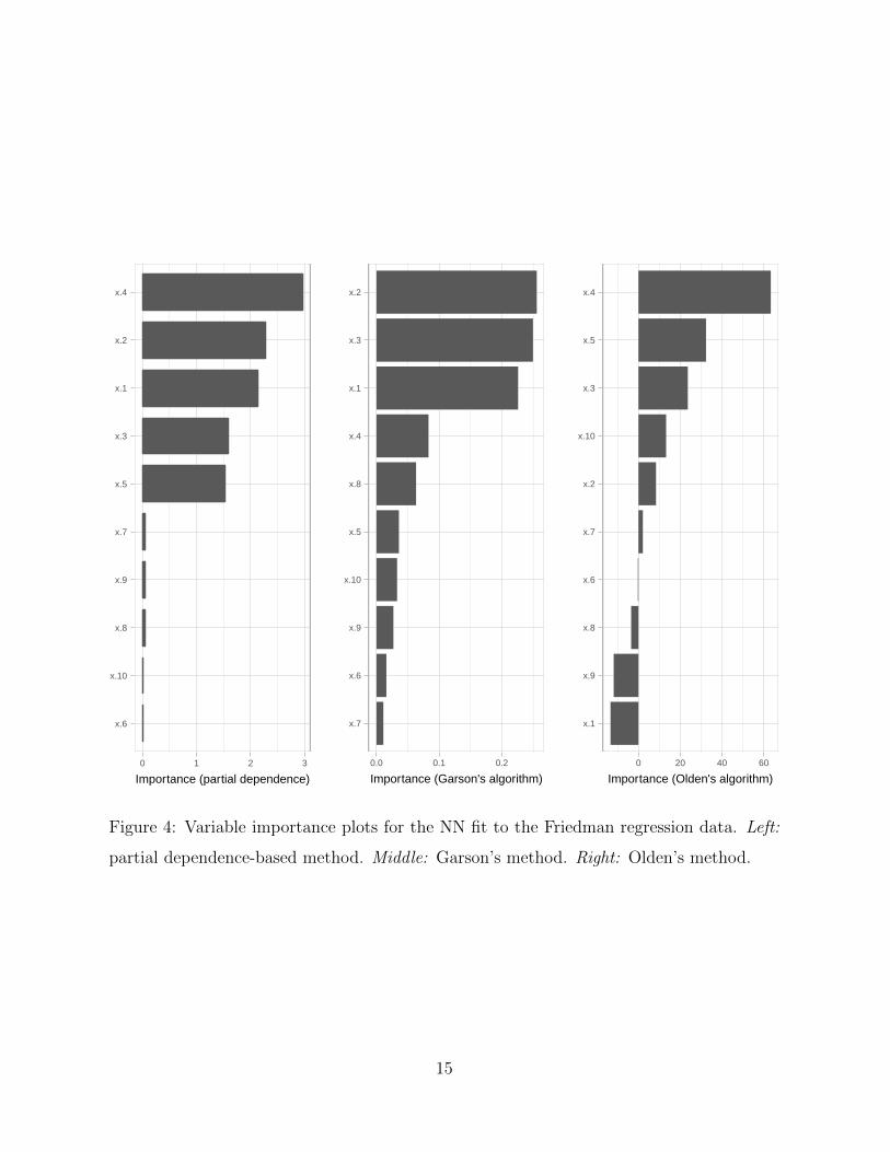
Variable importance plots are displayed in Figure 4. Notice how the Garson and Olden

algorithms incorrectly label some of the features not in the true model as “important”.

For example, the Garson algorithm incorrectly labels x8 (which is not included in the true

model) as more important than x5 (which is in the true model). Similarly, Oden’s method

incorrectly labels x10 as being more important than x2. Our method, on the other hand,

clearly labels all five of the predictors in the true model as the most important features in

the fitted NN.

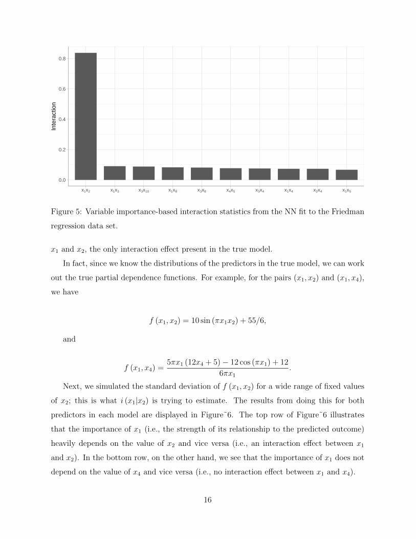
We also constructed the partial dependence functions for all pairwise interactions and

computed the interaction statistic discussed in Section 3.2. The top ten interaction statistics

are displayed in Figure 5. There is a clear indication of an interaction effect between features

14

x.6

x.10

x.8

x.9

x.7

x.5

x.3

x.1

x.2

x.4

0 1 2 3

Importance (partial dependence)

x.7

x.6

x.9

x.10

x.5

x.8

x.4

x.1

x.3

x.2

0.0 0.1 0.2

Importance (Garson's algorithm)

x.1

x.9

x.8

x.6

x.7

x.2

x.10

x.3

x.5

x.4

0 20 40 60

Importance (Olden's algorithm)

Figure 4: Variable importance plots for the NN fit to the Friedman regression data. Left:

partial dependence-based method. Middle: Garson’s method. Right: Olden’s method.

15

0.0

0.2

0.4

0.6

0.8

x1x2 x1x3 x3x10 x1x8 x3x8 x4x5 x3x4 x1x4 x2x4 x1x5

Inte

ract

ion

Figure 5: Variable importance-based interaction statistics from the NN fit to the Friedman

regression data set.

x1 and x2, the only interaction effect present in the true model.

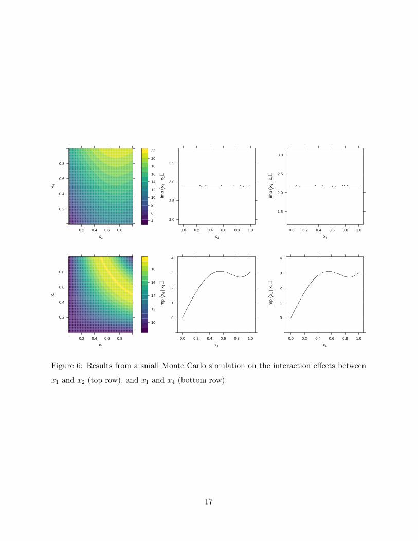
In fact, since we know the distributions of the predictors in the true model, we can work

out the true partial dependence functions. For example, for the pairs (x1, x2) and (x1, x4),

we have

f (x1, x2) = 10 sin (πx1x2) + 55/6,

and

f (x1, x4) =5πx1 (12x4 + 5)− 12 cos (πx1) + 12

6πx1.

Next, we simulated the standard deviation of f (x1, x2) for a wide range of fixed values

of x2; this is what i (x1|x2) is trying to estimate. The results from doing this for both

predictors in each model are displayed in Figure˜6. The top row of Figure˜6 illustrates

that the importance of x1 (i.e., the strength of its relationship to the predicted outcome)

heavily depends on the value of x2 and vice versa (i.e., an interaction effect between x1

and x2). In the bottom row, on the other hand, we see that the importance of x1 does not

depend on the value of x4 and vice versa (i.e., no interaction effect between x1 and x4).

16

x1

x 4

0.2

0.4

0.6

0.8

0.2 0.4 0.6 0.8

4

6

8

10

12

14

16

18

20

22

x1

imp

(x4

| x1)

2.0

2.5

3.0

3.5

0.0 0.2 0.4 0.6 0.8 1.0

x4

imp

(x1

| x4)

1.5

2.0

2.5

3.0

0.0 0.2 0.4 0.6 0.8 1.0

x1

x 4

0.2

0.4

0.6

0.8

0.2 0.4 0.6 0.8

10

12

14

16

18

x1

imp

(x4

| x1)

0

1

2

3

4

0.0 0.2 0.4 0.6 0.8 1.0

x4

imp

(x1

| x4)

0

1

2

3

4

0.0 0.2 0.4 0.6 0.8 1.0

Figure 6: Results from a small Monte Carlo simulation on the interaction effects between

x1 and x2 (top row), and x1 and x4 (bottom row).

17

4.1 Friedman’s H-statistic

An alternative measure for the strength of interaction effects is known as Friedman’s H-

statistic (Friedman & Popescu 2008). Coincidentally, this method is also based on the

estimated partial dependence functions of the corresponding predictors, but uses a different

approach.

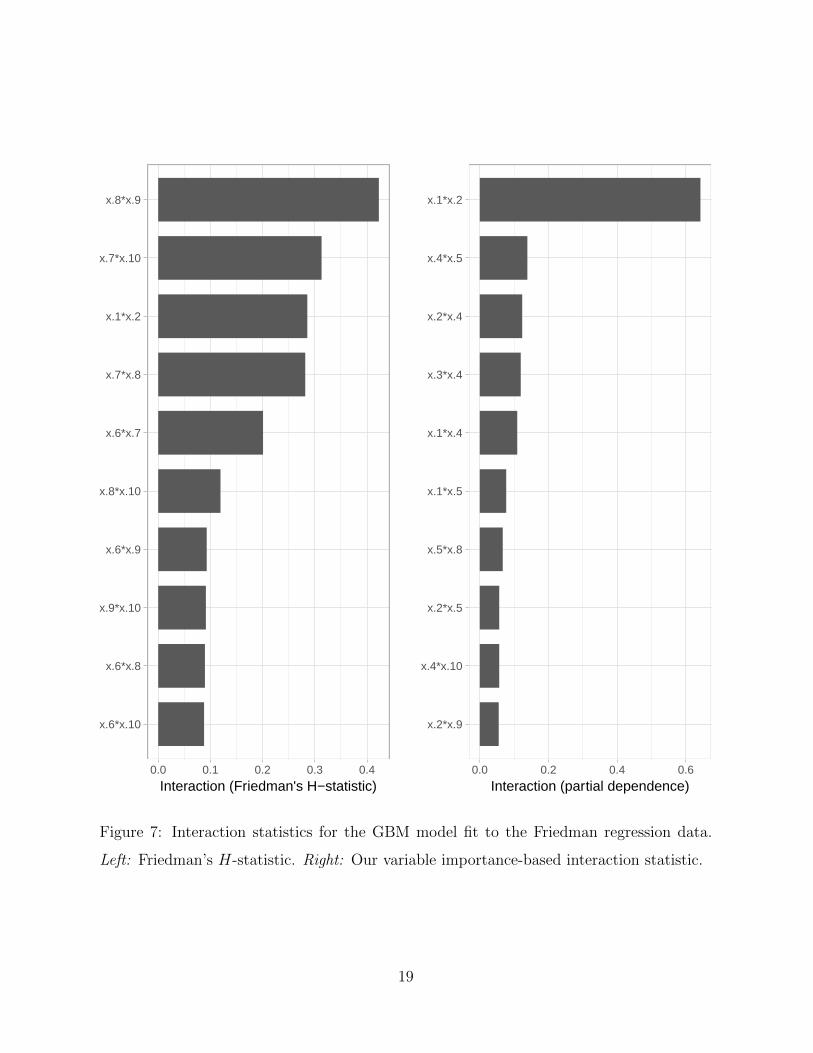
For comparison, we fit a GBM to the Friedman regression data from the previous

section. The parameters were chosen using 5-fold cross-validation. We used the R package

gbm (Ridgeway 2017) which has built-in support for computing Friedman’s H-statistic for

any combination of predictors. The results are displayed in Figure 7. To our surprise, the

H-statistic did not seem to catch the true interaction between x1 and x2. Instead, the H-

statistic ranked the pairs (x8, x9) and (x7, x10) as having the strongest interaction effects,

even though these predictors do not appear in the true model. Our variable importance-

based interaction statistic, on the other hand, clearly suggests the pair (x1, x2) as having

the strongest interaction effect.

5 Application to model stacking

In the Ames housing example, we used a GBM to illustrate the idea of using the partial

dependence function to quantify the importance of each predictor on the predicted outcome

(in this case, Log Sale Price). While the GBM model achieved a decent cross-validated

R2 of 91.54%, better predictive performance can often be attained by creating an ensemble

of learning algorithms. While GBMs are themselves ensembles, we can use a method

called stacking to combine the GBM with other cutting edge learning algorithms to form

a super learner (Wolpert 1992). Such stacked ensembles tend to outperform any of the

individual base learners (e.g., a single RF or GBM) and have been shown to represent an

asymptotically optimal system for learning (van der Laan et al. 2003).

For the Ames data set, in addition to the GBM, we trained and tuned a RF using 10-

fold cross-validation. The cross-validated predicted values from each of these models were

combined to form a n× 2 matrix, where n = 1460 is the number of training records. This

matrix, together with the observed values of Log Sale Price, formed the “level-one” data.

18

x.6*x.10

x.6*x.8

x.9*x.10

x.6*x.9

x.8*x.10

x.6*x.7

x.7*x.8

x.1*x.2

x.7*x.10

x.8*x.9

0.0 0.1 0.2 0.3 0.4

Interaction (Friedman's H−statistic)

x.2*x.9

x.4*x.10

x.2*x.5

x.5*x.8

x.1*x.5

x.1*x.4

x.3*x.4

x.2*x.4

x.4*x.5

x.1*x.2

0.0 0.2 0.4 0.6

Interaction (partial dependence)

Figure 7: Interaction statistics for the GBM model fit to the Friedman regression data.

Left: Friedman’s H-statistic. Right: Our variable importance-based interaction statistic.

19

Overall_Cond

Fireplace_Qu

Full_Bath

MS_SubClass

Total_Bsmt_SF

Garage_Area

First_Flr_SF

Garage_Cars

Kitchen_Qual

Bsmt_Qual

Year_Built

Exter_Qual

Gr_Liv_Area

Neighborhood

Overall_Qual

0.00 0.25 0.50 0.75 1.00

Scaled importance

Random forest

Lot_Area

Sale_Condition

BsmtFin_Type_1

Year_Remod_Add

Central_Air

Overall_Cond

MS_SubClass

Garage_Area

First_Flr_SF

Total_Bsmt_SF

Kitchen_Qual

Garage_Cars

Gr_Liv_Area

Neighborhood

Overall_Qual

0.00 0.25 0.50 0.75 1.00

Scaled importance

GBM

Exterior_1st

Lot_Area

Second_Flr_SF

Garage_Area

Full_Bath

Sale_Condition

First_Flr_SF

Year_Built

Garage_Cars

Functional

Overall_Cond

Total_Bsmt_SF

Neighborhood

Gr_Liv_Area

Overall_Qual

0.00 0.25 0.50 0.75 1.00

Scaled importance

Stacked ensemble

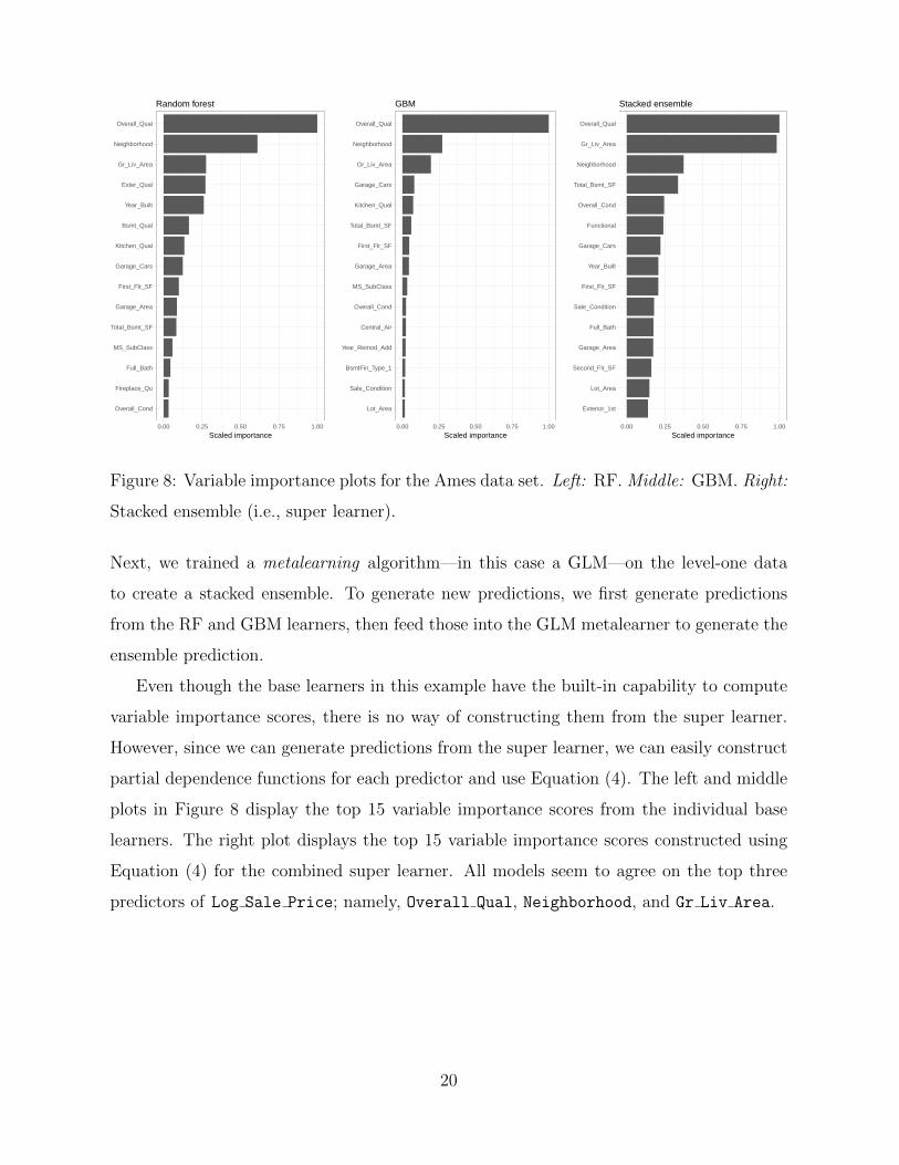
Figure 8: Variable importance plots for the Ames data set. Left: RF. Middle: GBM. Right:

Stacked ensemble (i.e., super learner).

Next, we trained a metalearning algorithm—in this case a GLM—on the level-one data

to create a stacked ensemble. To generate new predictions, we first generate predictions

from the RF and GBM learners, then feed those into the GLM metalearner to generate the

ensemble prediction.

Even though the base learners in this example have the built-in capability to compute

variable importance scores, there is no way of constructing them from the super learner.

However, since we can generate predictions from the super learner, we can easily construct

partial dependence functions for each predictor and use Equation (4). The left and middle

plots in Figure 8 display the top 15 variable importance scores from the individual base

learners. The right plot displays the top 15 variable importance scores constructed using

Equation (4) for the combined super learner. All models seem to agree on the top three

predictors of Log Sale Price; namely, Overall Qual, Neighborhood, and Gr Liv Area.

20

6 Application to automatic machine learning

The data science field has seen an explosion in interest over the last decade. However, the

supply of data scientists and machine learning experts has not caught up with the demand.

Consequently, many organizations are turning to automated machine learning (AutoML)

approaches to predictive modelling. AutoML has been a topic of increasing interest over

the last couple of years and open source implementations—like those in H2O and auto-

sklearn (Feurer et al. 2015)—have made it a simple and viable options for real supervised

learning problems.

Current AutoML algorithms leverage recent advantages in Bayesian optimization, meta-

learning, and ensemble construction (i.e., model stacking). The benefit, as compared to

the stacked ensemble formed in Section 5, is that AutoML frees the analyst from having to

do algorithm selection (e.g., “Do I fit an RF or GBM to my data?”) and hyperparameter

tuning (e.g., how many hidden layers to use in a DNN). While AutoML has great practical

potential, it does not automatically provide any useful interpretations—AutoML is not

automated data science (Mayo 2017). For instance, which variables are the most important

in making accurate predictions? How do these variables functionally related to the outcome

of interest? Fortunately, our approach can still be used to answer these two questions

simultaneously.

To illustrate, we used the R implementation of H2O’s AutoML algorithm to model

the airfoil self-noise data set (Lichman 2013) which are available from the University of

California Machine Learning Repository: https://archive.ics.uci.edu/ml/datasets/

airfoil+self-noise. These data are from a NASA experiment investigating different size

NACA 0012 airfoils at various wind tunnel speeds and angles of attack. The objective is to

accurately predict the scaled sound pressure level (dB) (scaled sound pressure level)

using frequency (Hz) (frequency), angle of attack (degrees) (angle of attack), chord

length (m) (chord length), free-stream velocity (m/s) (free stream velocity), and suc-

tion side displacement thickness (m) (suction side displacement thickness). H2O’s

current AutoML implementation trains and cross-validates an RF, an extremely-randomized

forest (XRF) (Geurts et al. 2006), a random grid of GBMs, a random grid of DNNs, and

then trains a stacked ensemble using the approach outlined in Section 5. We used 10-fold

21

cross-validation and RMSE for the validation metric. Due to hardware constraints, we used

a max run time of 15 minutes (the default is one hour). The final model consisted of one

DNN, a random grid of 37 GBMs, one GLM, one RF, one XRT, and two stacked ensembles.

The final stacked ensemble achieved a 10-fold cross-validated RMSE and R-squared of 1.43

and 95.68, respectively.

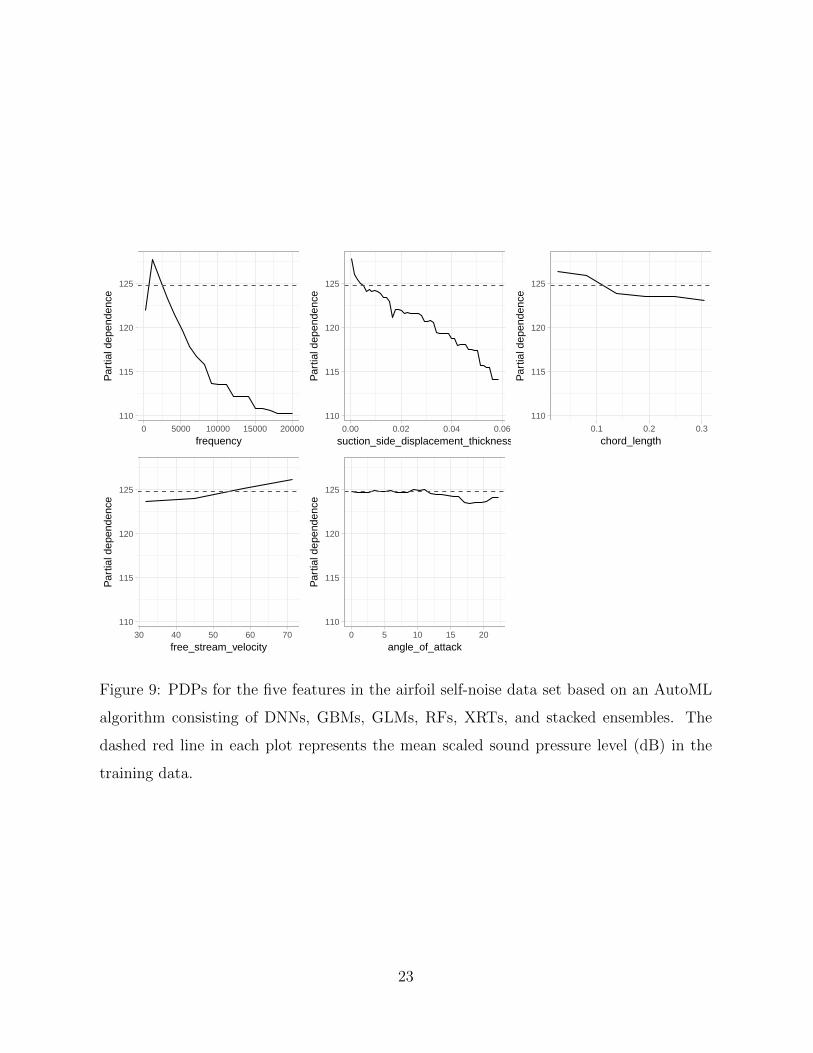
Since predictions can be obtained from the automated stacked ensemble, we can easily

apply Algorithm 1 and construct PDPs for all the features; these are displayed in Figure

9. It seems frequency (Hz) and suction side displacement thickness (m) have a strong

monotonically decreasing relationship with scaled sound pressure level (dB). They also

appear to be more influential than the other three. Using Equation (4), we computed the

variable importance of each of the five predictors which are displayed in Table 1.

Variable Importance

Angle of attack (degrees) 0.4888482

Free stream velocity (m/s) 1.1158569

Chord length (m) 1.4168613

Suction side displacement thickness (m) 3.3389105

Frequency (Hz) 5.4821362

Table 1: Partial dependence-based variable importance scores for the five predictors in

the airfoil self-noise data set based on an AutoML algorithm consisting of DNNs, GBMs,

GLMs, RFs, XRTs, and stacked ensembles.

7 Discussion

We have discussed a new variable importance measure that is (i) suitable for use with any

supervised learning algorithm, provided new predictions can be obtained, (ii) model-based

and takes into account the effect of all the features in the model, (iii) consistent and has

the same interpretation regardless of the learning algorithm employed, and (iv) has the

potential to help identify possible interaction effects. Since our algorithm is model-based

it requires that the model be properly trained and tuned to achieve optimum performance.

22

110

115

120

125

0 5000 10000 15000 20000

frequency

Par

tial d

epen

denc

e

110

115

120

125

0.00 0.02 0.04 0.06

suction_side_displacement_thickness

Par

tial d

epen

denc

e

110

115

120

125

0.1 0.2 0.3

chord_length

Par

tial d

epen

denc

e

110

115

120

125

30 40 50 60 70

free_stream_velocity

Par

tial d

epen

denc

e

110

115

120

125

0 5 10 15 20

angle_of_attack

Par

tial d

epen

denc

e

Figure 9: PDPs for the five features in the airfoil self-noise data set based on an AutoML

algorithm consisting of DNNs, GBMs, GLMs, RFs, XRTs, and stacked ensembles. The

dashed red line in each plot represents the mean scaled sound pressure level (dB) in the

training data.

23

While this new approach appears to have high utility, more research is needed to determine

where its deficiencies may lie. For example, outliers in the feature space can cause abnor-

mally large fluctuations in the partial dependence values f (xi) (i = 1, 2, . . . , k). Therefore,

it may be advantageous to use more robust measures of spread to describe the variability in

the estimated partial dependence values; a reasonable choice would be the median absolute

deviation which has a finite sample breakdown point of bk/2c /k. It is also possible to re-

place the mean in step (3) of Algorithm 1 with a more robust estimate such as the median

or trimmed mean. Another drawback is the computational burden imposed by Algorithm

1 on large data sets, but this can be mitigated using the methods discussed in Greenwell

(2017).

All the examples in this article were produced using R version 3.4.0 (R Core Team

2017); a software environment for statistical computing. With the exception of Figure 6,

all graphics were produced using the R package ggplot2 (Wickham 2009); Figure 6 was

produced using the R package lattice (Sarkar 2008).

SUPPLEMENTARY MATERIAL

R package: The R package ‘vip‘, hosted on GitHub at https://github.com/AFIT-R/

vip, contains functions for computing variable importance scores and constructing

variable importance plots for various types of fitted models in R using the partial

dependence-based approach discussed in this paper.

R code: The R script ‘vip-2018.R‘ contains the R code to reproduce all of the results and

figures in this paper.

References

Breiman, L. (1996), ‘Bagging predictors’, Machine Learning 8(2), 209–218.

URL: https://doi.org/10.1023/A:1018054314350

Breiman, L., Friedman, J. & Charles J. Stone, R. A. O. (1984), Classification and Regression

Trees, The Wadsworth and Brooks-Cole statistics-probability series, Taylor & Francis.

24

Cleveland, W. S. (1979), ‘Robust locally weighted regression and smoothing scatterplots’,

Journal of the American Statistical Association 74(368), 829–836.

Cock, D. D. (2011), ‘Ames, iowa: Alternative to the boston housing data as an end of

semester regression project’, Journal of Statistics Education 19(3), 1–15.

URL: http://ww2.amstat.org/publications/jse/v19n3/decock.pdf

Feurer, M., Klein, A., Eggensperger, K., Springenberg, J., Blum, M. & Hutter, F. (2015),

Efficient and robust automated machine learning, in C. Cortes, N. D. Lawrence, D. D.

Lee, M. Sugiyama & R. Garnett, eds, ‘Advances in Neural Information Processing

Systems 28’, Curran Associates, Inc., pp. 2962–2970.

URL: http://papers.nips.cc/paper/5872-efficient-and-robust-automated-machine-

learning.pdf

Friedman, J. H. (1991a), ‘Multivariate adaptive regression splines’, The Annals of Statistics

19(1), 1–67.

URL: https://doi.org/10.1214/aos/1176347963

Friedman, J. H. (1991b), ‘Multivariate adaptive regression splines’, The Annals of Statistics

19(1), 1–67.

URL: https://doi.org/10.1214/aos/1176347963

Friedman, J. H. (2001), ‘Greedy function approximation: A gradient boosting machine’,

The Annals of Statistics 29, 1189–1232.

URL: https://doi.org/10.1214/aos/1013203451

Friedman, J. H. & Popescu, B. E. (2008), ‘Predictive learning via rule ensembles’, Annals

of Applied Statistics 2(3), 916–954.

URL: https://doi.org/10.1214/07-aoas148

Garson, D. G. (1991), ‘Interpreting neural-network connection weights’, Artificial Intelli-

gence Expert 6(4), 46–51.

Gedeon, T. (1997), ‘Data mining of inputs: Analysing magnitude and functional measures’,

25

International Journal of Neural Systems 24(2), 123–140.

URL: https://doi.org/10.1007/s10994-006-6226-1

Geurts, P., Ernst, D. & Wehenkel, L. (2006), ‘Extremely randomized trees’, Machine Learn-

ing 63(1), 3–42.

URL: https://doi.org/10.1007/s10994-006-6226-1

Goh, A. (1995), ‘Back-propagation neural networks for modeling complex systems’, Artifi-

cial Intelligence in Engineering 9(3), 143–151.

Goldstein, A., Kapelner, A., Bleich, J. & Pitkin, E. (2015), ‘Peeking inside the black box:

Visualizing statistical learning with plots of individual conditional expectation’, Journal

of Computational and Graphical Statistics 24(1), 44–65.

URL: https://doi.org/10.1080/10618600.2014.907095

Greenwell, B. M. (2017), ‘pdp: An r package for constructing partial dependence plots’,

The R Journal 9(1), 421–436.

URL: https://journal.r-project.org/archive/2017/RJ-2017-016/index.html

Harrison, D. & Rubinfeld, D. L. (1978), ‘Hedonic housing prices and the demand for clean

air’, Journal of Environmental Economics and Management 5(1), 81–102.

URL: https://doi.org/10.1016/0095-0696(78)90006-2

Hastie, T., Tibshirani, R. & Friedman, J. (2009), The Elements of Statistical Learning:

Data Mining, Inference, and Prediction, Second Edition, Springer Series in Statistics,

Springer-Verlag.

Kuhn, M. (2017), AmesHousing: The Ames Iowa Housing Data. R package version 0.0.3.

URL: https://CRAN.R-project.org/package=AmesHousing

Kuhn, M. & Johnson, K. (2013), Applied Predictive Modeling, SpringerLink : Bucher,

Springer New York.

Lichman, M. (2013), ‘UCI machine learning repository’.

URL: http://archive.ics.uci.edu/ml

26

Mayo, M. (2017), ‘The current state of automated machine learning’.

URL: https://www.kdnuggets.com/2017/01/current-state-automated-machine-

learning.html

Olden, J. D., Joy, M. K. & Death, R. G. (2004), ‘An accurate comparison of methods

for quantifying variable importance in artificial neural networks using simulated data’,

Ecological Modelling 178(3), 389–397.

R Core Team (2017), R: A Language and Environment for Statistical Computing, R Foun-

dation for Statistical Computing, Vienna, Austria.

URL: https://www.R-project.org/

Ridgeway, G. (2017), gbm: Generalized Boosted Regression Models. R package version 2.1.3.

URL: https://CRAN.R-project.org/package=gbm

Sarkar, D. (2008), Lattice: Multivariate Data Visualization with R, Springer, New York.

ISBN 978-0-387-75968-5.

URL: http://lmdvr.r-forge.r-project.org

The H2O.ai team (2017), h2o: R Interface for H2O. R package version 3.14.0.3.

URL: https://CRAN.R-project.org/package=h2o

van der Laan, M. J., Polley, E. C. & Hubbard, A. E. (2003), ‘Super learner’, Statistical

Applications in Genetics and Molecular Biology 6(1).

Venables, W. N. & Ripley, B. D. (2002), Modern Applied Statistics with S, 4th edn, Springer-

Verlag, New York.

URL: http://www.stats.ox.ac.uk/pub/MASS4

Wickham, H. (2009), ggplot2: Elegant Graphics for Data Analysis, Springer-Verlag New

York.

URL: http://ggplot2.org

Wolpert, D. H. (1992), ‘Stacked generalization’, Neural Networks 5, 241–259.

27