A sieve algorithm based on overlattices

LMS J. Comput. Math. 17 (Special issue A) (2014) 49–70 C© 2014 Authors

doi:10.1112/S1461157014000229

A sieve algorithm based on overlattices

Anja Becker, Nicolas Gama and Antoine Joux

AbstractIn this paper, we present a heuristic algorithm for solving exact, as well as approximate, shortestvector and closest vector problems on lattices. The algorithm can be seen as a modified sievingalgorithm for which the vectors of the intermediate sets lie in overlattices or translated cosetsof overlattices. The key idea is hence no longer to work with a single lattice but to move theproblems around in a tower of related lattices. We initiate the algorithm by sampling very shortvectors in an overlattice of the original lattice that admits a quasi-orthonormal basis and hencean efficient enumeration of vectors of bounded norm. Taking sums of vectors in the sample, weconstruct short vectors in the next lattice. Finally, we obtain solution vector(s) in the initiallattice as a sum of vectors of an overlattice. The complexity analysis relies on the Gaussianheuristic. This heuristic is backed by experiments in low and high dimensions that closely reflectthese estimates when solving hard lattice problems in the average case.

This new approach allows us to solve not only shortest vector problems, but also closestvector problems, in lattices of dimension n in time 20.3774n using memory 20.2925n. Moreover,the algorithm is straightforward to parallelize on most computer architectures.

1. Introduction

Hard lattice problems, such as the shortest vector problem (SVP) and the closest vectorproblem (CVP), have a long-standing relationship to number theory and cryptology. In numbertheory, they can for example be used to find Diophantine approximations. In cryptology,they were used as cryptanalytic tools for a long time, first through a direct approach asin [20] and then more indirectly using Coppersmith’s small roots algorithms [8, 9]. Morerecently, these hard problems have also been used to construct cryptosystems. Lattice-basedcryptography is also a promising area due to the simple additive, parallelizable structure ofa lattice. The two basic hard problems SVP and CVP are known to be NP-hard† to solveexactly [1, 22] and also NP-hard to approximate [10, 26] within at least constant factors. Thetime complexity of known algorithms that find the exact solution is at least exponential inthe dimension of the lattice. These algorithms also serve as subroutines for strong polynomialtime approximation algorithms. Algorithms for the exact problem hence enable us to chooseappropriate parameters.

A shortest vector can be found by enumeration [21, 36], sieving [3, 28, 31, 38] or theVoronoi-cell algorithm [27]. Enumeration uses a negligible amount of memory and its running

time is between nO(n) and 2O(n2) depending on the amount and quality of the preprocessing.Probabilistic sieving algorithms, as well as the deterministic Voronoi-cell algorithm are simplyexponential in time and memory. A closest vector can be found by enumeration and by theVoronoi-cell algorithm; however, to the best of our knowledge, no sieve algorithm is known

Received 27 February 2014; revised 23 May 2014.

2010 Mathematics Subject Classification 11H99 (primary), 11Y16, 68T20, 90C59 (secondary).

Contributed to the Algorithmic Number Theory Symposium XI, GyeongJu, Korea, 6–11 August 2014.

Part of this work was supported by the Swiss National Science Foundation under grant numbers 200021-126368 and 200020-153113.

†Under randomized reductions in the case of SVP.

https://www.cambridge.org/core/terms. https://doi.org/10.1112/S1461157014000229Downloaded from https://www.cambridge.org/core. IP address: 65.21.228.167, on 02 Dec 2021 at 11:55:05, subject to the Cambridge Core terms of use, available at

https://www.cambridge.org/core/terms

https://doi.org/10.1112/S1461157014000229

https://www.cambridge.org/core

50 a. becker, n. gama and a. joux

to provably solve CVP instances, and it would be interesting to study other sieve algorithmswhich also work in the CVP case. Table 1 presents the complexities of currently known SVPand CVP algorithms including our new algorithm. In particular, it shows that the asymptotictime complexity of our new approach (slightly) outperforms the complexity of the best pre-existing sieving algorithm and that, as a bonus, it can for the same price serve as a CVPalgorithm. The high memory requirement limits the size of accessible dimensions, for examplewe need 3 TB of storage in dimension 90 which we divide into 25 groups of 120 GB in RAM,and we would need twice as much in dimension 96. For this reason, the algorithm, as well asother classical sieving techniques, is in practice not competitive with the fastest memorylessmethods such as pruned enumeration or aborted BKZ. However, our experiments suggest thatdespite the higher memory requirements, the sequential running time of our algorithm is ofthe same order of magnitude as the Gauss sieve, but with an algorithm easier to parallelize.

A long-standing open question was to find ways to decrease the complexity of enumeration-based algorithms to a single exponential time complexity. On an LLL- or BKZ-reducedbasis [24, 36] the running time of Schnorr and Euchner’s enumeration is doubly exponentialin the dimension. If we further reduce the basis to an HKZ-reduced basis [23], the complexitybecomes 2O(n logn) [18, 21]. Enumeration would become simply exponential if a quasi-orthonormal basis, as defined in § 2, could be found. Unfortunately, most lattices do not possesssuch a favorable quasi-orthonormal basis. Also for random lattices the lower bound on theRankin invariant is of size 2Θ(n logn) and determines the minimal complexity for enumerationthat operates exclusively on the original lattice. We provide a more detailed discussion in § 2.

Our approach circumvents this problem by making use of overlattices that admit a quasi-orthonormal basis. These overlattices are found in polynomial time by an algorithm relying onthe structural reduction introduced by [14], as described in § 3.2. Once we have an overlatticeand its quasi-orthonormal basis, we may efficiently enumerate short vectors at a constantfactor of the first minimum in the overlattice. Our main task is to turn these small samplesinto a solution vector in the initial lattice. The construction is very similar to an observation byMordell [30] in 1935 which presented the first algorithmic proof of Minkowski’s inequality usingonly finite elements. Namely, he observed that given a lattice Li and an overlattice Li+1 ⊃ Lisuch that [Li+1 : Li] = r, in any pool of at least r + 1 short vectors of Li+1, there exist atleast two vectors whose difference is a short non-zero vector in Li. This construction has alsobeen implicitly used in worst-case to average-case reductions, where a short overlattice basisis used to sample a pool of short Gaussian overlattice vectors, which are then combined by anSIS (short integer solution) oracle into polynomially longer vectors of the original lattice. Inour setting, the overlattice basis is quasi-orthonormal, which allows an efficient enumeration

Table 1. Complexity of currently known SVP/CVP algorithms.

Algorithm Time Memory CVP SVP

Kannan enumeration [18] nn/2+o(n) poly(n) X Proven

nn/(2e)+o(n) poly(n) X Proven

Voronoi cell [27] 22n 2n X X Proven

ListSieve birthday [33] 22.465n+o(n) 21.233n+o(n) × X Proven

GaussSieve [28] 20.415n+o(n)? 20.2075n+o(n)? ? X Heuristic

Nguyen–Vidick sieve [31] 20.415n+o(n) 20.2075n+o(n) × X Heuristic

WLTB sieve [38] 20.3836n+o(n) 20.2557n+o(n) × X Heuristic

Three-level sieve [39] 20.3778n+o(n) 20.2833n+o(n) × X Heuristic

Our algorithm from 20.4150n 20.2075n X X Heuristic

to 20.3774n 20.2925n



https://doi.org/10.1112/S1461157014000229


a sieve algorithm based on overlattices 51

of the shortest overlattice vectors. These vectors are then combined to the shortest vectors ofthe original lattice by a concrete, albeit exponential time, algorithm.

The new algorithm solves SVP and CVP for random lattices in the spirit of a sievingalgorithm, except that intermediate vectors lie in overlattices or cosets of overlattices whosegeometry varies from dense lattices to quasi-orthogonal lattices. Alternatively, the algorithmcan be viewed as an adaptation of the representation technique that solves knapsackproblems [4] and decoding problems [5, 25] to the domain of lattices. Due to the richerstructure of lattices, the adaptation is far from straightforward. To give a brief analogy,instead of searching for a knapsack solution, assume that we want to find a short vectorin an integer lattice. An upper bound on the Euclidean norm of the solution vector providesa geometric constraint, which induces a very large search space. The short vector we seekcan be decomposed in many ways as the sum of two shorter vectors with integer coefficients.Assuming that these sums provide N different representations of the same solution vector,we can then choose any arbitrary constraint which eliminates all but a fraction ≈1/N of allrepresentations. With this additional constraint, the solution vector can still be efficientlyfound, in a search space reduced by a factor N . From a broader perspective, this techniquecan be used to transform a problem with a hard geometric constraint, like short lattice vectors,into an easier subproblem, like short integer vectors (because Zn has an orthonormal basis),together with a custom additional constraint which is in general linear or modular, allowingan efficient recombination of the solutions to the subproblems. The biggest challenge is tobootstrap the algorithm by finding suitable and easier subproblems using overlattices. Wepropose a method that achieves this thanks to a well-chosen overlattice allowing an efficientdeterministic enumeration of vectors of bounded norm. In this way, we can compute a startingset of vectors that is used to initiate a sequence of recombinations that ends up solving theproblem initially considered.

Our contribution. We present a new heuristic algorithm for the exact SVP and CVP forn-dimensional lattices using a tower of k overlattices Li, where L = L0 ⊆ . . . ⊆ Lk. In thistower, we choose the lattice Lk at the bottom of the tower in a way that ensures that we canefficiently compute a sufficiently large pool of very short vectors in Lk. Starting from this poolof short vectors, we move from each lattice of our tower to the one above using summation ofvectors while controlling the growth of norms.

For random lattices and under heuristic assumptions, two Li+1-vectors sum up to anLi-vector with probability 1/αn, where vol(Li)/vol(Li+1) = αn > 1. We allow the normto increase by a moderate factor α in each step, in order to preserve the size of our pool ofavailable vectors per lattice in our tower.

Our method can be used to find vectors of bounded norm in a lattice L or, alternatively,in a coset x + L, x /∈ L. Thus, in contrast to classical sieving techniques, it allows us tosolve both SVP or CVP, and more generally, to enumerate all lattice points within a ball offixed radius. The average running time in the asymptotic case is 20.3774n, requiring a memoryof 20.2925n. It is also possible to choose different time–memory tradeoffs and devise sloweralgorithms that need less memory. We report our experiments on random lattices and SVPchallenges of dimension 40 to 90, whose results confirm our theoretical analysis and show thatthe algorithm works well in practice. We also study various options to parallelize the algorithmand show that parallelization works well on a wide range of computer architectures.

2. Background and notation

Lattices and cosets. A lattice L of dimension n is a discrete subgroup of Rm than spans ann-dimensional linear subspace. A lattice can be described as the set of all integer combinations



https://doi.org/10.1112/S1461157014000229



{∑ni=1 αibi |αi ∈ Z} of n linearly independent vectors bi of Rm. Such vectors b1, . . . , bn

are called a basis of L. The volume of the lattice L is the volume of span(L)/L, and canbe computed as

√det(BBt), for any basis B. Any lattice has a shortest non-zero vector of

Euclidean length λ1(L) which can be upper-bounded by Minkowski’s theorem as λ1(L) 6√n vol(L)1/n. We call a coset of L a translation x + L = {x + v |v ∈ L} of L by a vector

x ∈ span(L).

Overlattice and index. A lattice L′ of dimension n such that L ⊆ L′ is called an overlatticeof L. The quotient group L′/L is a finite abelian group of order vol(L)/vol(L′) = [L′ : L].

Hyperballs. Let Balln(R) denote the ball of radius R in dimension n, where we omit n if itis implied by the context. The volume Vn of the n-dimensional ball of radius 1 and the radiusrn of the n-dimensional ball of volume 1 are respectively:

Vn =

√πn

Γ(n/2 + 1)and rn = V −1/n

n =

√n

2πe(1 + o(1)).

Gaussian heuristic. In many cases, when we wish to estimate the number of lattice pointsin a ‘nice enough’ set S, we can use the Gaussian heuristic. In this paper, we will quantify theGaussian heuristic as follows:

Heuristic 2.1 (Gaussian heuristic). There exists a constant† GH > 1 such that for all thelattices L and all the sets S that we consider in this paper, the number of points in S ∩ Lsatisfies:

1

GH· vol(S)

vol(L)6 #(S ∩ L) 6 GH ·

vol(S)

vol(L).

In fact, it can be proved that for any bounded measurable set S, the expectation, overrandom unit volume lattices drawn from the Haar distribution [2], of the number of non-zeropoints is always the volume of S. Also, for any fixed lattice of unit volume and any fixedbounded measurable set S, the expectation of the number of lattice points in t+S for uniformt modulo L is exactly vol(S). However, fewer results are known about the standard deviation,or whether these distributions are concentrated enough around the expectation so that almostall instances satisfy the upper and lower bounds.

In this paper, the geometry of lattices varies between random integer lattices of large enoughvolume and quasi-orthonormal lattices. We will assume that in these lattices, the length λ1

of the shortest vector is the one given by the Gaussian heuristic, that is, the radius of a ballof volume vol(L): λ1(L) ≈ rn · n

√vol(L). Furthermore, the sets S we consider in this paper

are either balls of radius larger than√

3/2 rnn√

vol(L), and whose center is uniform modulothe lattice (that is, far from 0), or the intersection of two such balls whose centers are closeenough. In these cases, our experiments indicate that the number of lattice points in these setsis almost always between 50% and 110% of vol(S)/vol(L), thus Heuristic 2.1 holds in practicefor GH = 2.

Gram–Schmidt orthogonalization (GSO). The GSO of a non-singular square matrix B isthe unique decomposition as B = µ·B∗, where µ is a lower triangular matrix with unit diagonaland B∗ consists of mutually orthogonal rows. For each i ∈ [1, n], we call πi the orthogonalprojection over span(b1, . . . , bi−1)⊥. In particular, one has πi(bi) = b∗i , which is the ith row ofB∗. We use the notation B[i,j] for the projected block [πi(bi), . . . , πi(bj)].

†The algorithms and proofs would also work with GH = poly(n) or GH = (1 + ε)n, giving slightly worsecomplexities.



https://doi.org/10.1112/S1461157014000229



Rankin factor and quasi-orthonormal basis. Let B be an n-dimensional basis of a latticeL, and j 6 n. We call the ratio

γn,j(B) =vol(B[1,j])

vol(L)j/n=

vol(L)(n−j)/n

vol(πj+1(L))

the Rankin factor of B with index j. The well-known Rankin invariants of the lattice, γn,j(L),introduced by Rankin [34], are simply the squares of the minimal Rankin factors of index jover all bases of L. This allows us to define a quasi-orthonormal basis.

Definition 2.2 (Quasi-orthonormal basis). A basis B is quasi-orthonormal if and only ifits Rankin factors satisfy 1 6 γn,j(B) 6 n for all j ∈ [1, n].

In the above definition, we chose the upper bound n over a general poly(n) only because weare able to achieve this factor. More generally, any polynomial function would be sufficient forthe asymptotical analysis and for the running time. For example, any real triangular matrixwith identical diagonal coefficients forms a quasi-orthogonal basis. More generally, any basiswhose ‖b∗i ‖ are almost equal is quasi-orthogonal. This is a very strong notion of reduction, since

average LLL-reduced or BKZ-reduced bases only achieve a 2O(n2) Rankin factor and HKZ-reduced bases of random lattices have a 2O(n logn) Rankin factor. Finally, Rankin’s invariantsare lower-bounded [6, 13, 37] by 2Θ(n logn) for almost all lattices†, which means that onlylattices in a tiny subclass possess a quasi-orthonormal basis.

Schnorr–Euchner enumeration. Given a basis B of an integer lattice L ⊆ Rn, the Schnorr–Euchner enumeration algorithm [36] allows us to us enumerate all vectors of Euclidean norm6 R in the bounded coset C = (z + L) ∩ Balln(R) where z ∈ Rn. The running time of thisalgorithm is

TSE =

n∑i=1

#(πn+1−i(z + L) ∩ Balli(R)), (2.1)

which is equivalent to

TSE ≈n∑i=1

vol(Balli(R))

vol(πn+1−i(L))(2.2)

under Heuristic 2.1. The last term in the sums (2.1) and (2.2) denotes the number of solutions#C. Thus, the complexity of enumeration is approximately TSE ≈ O(#C) ·maxj∈[1,n]γn,j(B).This is why a reduced basis of smallest Rankin factor is favorable. The lower bound onRankin’s invariant of γn,n/2(L) = 2Θ(n logn) for most lattices therefore determines the minimalcomplexity of enumeration that is achievable while working with the original lattice, providedthat one can actually compute a basis of L minimizing the Rankin factors, which is also NP-hard. If the input basis is quasi-orthonormal, the upper bound γn,j(B) 6 n from Definition 2.2

implies that the enumeration algorithm runs in time O(#C), which is optimal. Withoutknowledge of a good basis one can aim to decompose the problem into more favorable casesthat finally allow us to apply the Schnorr–Euchner algorithm as we describe below.

3. Enumeration of short vectors by intersection of hyperballs

This section presents the new algorithm that enumerates βn shortest vectors in any cosett + L of a lattice L for a constant β ≈

√3/2. It can be used to solve the NP-hard problems

†γ2n,n(L) > (n/12)n with probability ≈1 on random real lattices of volume 1 drawn from the Haardistribution.



https://doi.org/10.1112/S1461157014000229



SVP, CVP, ApproxSVPβ and ApproxCVPβ : given a lattice L, the SVP can be reduced toenumerating vectors of Euclidean norm O(λ1(L)) in the coset 0 + L while a CVP instancecan be solved by enumerating vectors of norm at most dist(t,L) in the coset −t + L. Thesebounded cosets, (t + L) ∩ Balln(R) for suitable radius R, can be constructed in an iterativeway by use of overlattices. The searched vectors are expressed as a sum of short vectors ofsuitable translated overlattices of smaller volume. The search for a unique element in a latticeas required in the SVP or CVP is delegated to the problem of enumerating bounded cosets.Any non-trivial element found by our algorithm is naturally a solution to the correspondingApproxSVPβ or ApproxCVPβ .

We present the new algorithm solving lattice problems based on intersections of hyperballs in§ 3.1 and the generic initialization of our algorithm as described in § 3.2. Finally, § 3.3 describesthe cost of the first step in the algorithm.

3.1. General description of the new algorithm

Assume that we are given a tower of k = O(n) lattices Li ⊂ Rn of dimension n where Li ⊆ Li+1

and the volume of any two consecutive lattices differs by a factor N = dαne ∈ N>1. We alsoassume that the bottom lattice Lk permits an efficient enumeration of the βn shortest vectorsin any coset t + Lk for 1 < β <

√3/2. The ultimate goal is to find the βn shortest vectors in

some coset t0 +L0 of L0. We postpone how to find suitable lattices Li, i > 1, to the followingtwo sections.

We also assume in this section, that the Gaussian heuristic (Heuristic 2.1) holds. Under thisassumption, the problem of finding the βn shortest elements in some coset t + L is roughlyequivalent to enumerating all lattice vectors of L in the ball of radius β · rn · n

√vol(L) centered

at −t ∈ Rn.Each step for i = k − 1 down to 0 of the algorithm is based on the following intuition: we

are given the ≈βn shortest vectors vj in ti/2 +Li+1. By summation, we can then find vectors(vj + vl)j6l that lie in ti + Li+1. We select those which actually lie in ti + Li and have normsmall enough, and consider them as the input pool for the next step. For suitable parameters,namely α small enough and β large enough, we thus recover the ≈βn shortest vectorsof ti + Li.

More precisely, for each i ∈ [0, k], we call Ci the bounded coset Ci that contains the βn

shortest vectors of the coset ti + Li where ti = t0/2i ∈ Rn. More formally, let us define

Ri = β · rn n√

vol(Li) and Ci = (ti + Li) ∩ Ball(0, Ri)

such that

#Ci ≈ vol(Ball(Ri))/vol(Li) = βn,

which follows from Heuristic 2.1. In addition, we recall that

Li ⊂ Li+1 where vol(Li)/vol(Li+1) = dαne.

In order to enumerate C0, our algorithm successively enumerates Ci, starting from i = kdown to zero; Figure 1 illustrates the sequence of enumerated lists.

During the construction of the tower of lattices, which is studied in the next sections,we already ensure that Ck is easy to obtain. We now explain how we can compute Ci−1

from Ci. To do this, we compute all sums x + y of vector pairs of Ci × Ci which satisfy



https://doi.org/10.1112/S1461157014000229



C0

Ci

Enumerate Ck

+ check (3.1), (3.2)

+ check (3.1), (3.2)

Figure 1. Iterative creation of lists.

the conditions

x + y ∈ ti−1 + Li−1 and (3.1)

‖x + y‖ 6 β · rn · n√

vol(Li−1). (3.2)

This means that we collect the βn shortest vectors of the coset Ci−1 = ti−1 + Li−1 by goingthrough Ci = ti + Li. In practice, an equivalent way to check if condition (3.1) holds, is touse an efficient computation for the map ϕi−1 : Ci → Li/Li−1, z → z − ti mod Li−1 and toverify that ϕi−1(x) + ϕi−1(y) = 0. Algorithm 1 summarizes our approach.

Algorithm 1 Coset enumeration

Constants: α ≈√

4/3, β ≈√

3/2Parameters: k

Input: An LLL-reduced basis B of L0 and a center t ∈ RnOutput: Elements of t + L0 of norm 6 R0 = βrnvol(L0)1/n

1: Randomize the input target by sampling t0 ∈ t+L. Use, for example, a discrete Gaussiandistribution of parameter

√n‖B∗‖. This defines all the sub-targets ti = t0/2

i

2: Compute a tower of lattices L0, . . . ,Lk by use of Algorithm 3 such that– L0 ⊂ L1 ⊂ ... ⊂ Lk and vol(Li)/vol(Li−1) = N = dαne– lattice enumeration is easy on Lk– testing morphisms ϕi−1 from ti + Li to Li/Li−1 are efficient to evaluate.

3: Enumerate bottom coset Ck (with Schnorr–Euchner)4: for i = k − 1 downto 0 do5: Ci ← Merge(Ci+1, ϕi, Ri = βrnvol(Li)1/n) (Algorithm 2)6: end for7: return C0

A naive implementation of the merge routine that creates Ci−1 from Ci would just runthrough the β2n pairs of vectors from Ci × Ci, and eliminate those that do not satisfy theconstraints (3.1) and (3.2). By regrouping the elements of Ci into αn buckets, according totheir value modulo Li−1, condition (3.1) implies that each element of Ci only needs to be pairedwith the elements of a single bucket (see Algorithm 2). Heuristic 2.1 implies that each bucketcontains at most GH(β/α)n elements, therefore the merge operation can then be performedin time G2

H(β2/α)n.

Complexity and constraints for parameters α and β. We now prove the complexity andcorrectness of Algorithm 2.



https://doi.org/10.1112/S1461157014000229



Algorithm 2 Merge by collision

/∗ Efficiently find pairs of vectors of Ci+1 s.t. their sum is in Ci∗/

/∗ Ci denotes (ti + Li) ∩ Ball(Ri)∗/

Input: The bounded coset Ci+1, a testing morphism ϕi and a radius RiOutput: The bounded coset Ci

1: Ci ← ∅2: Reorganize Ci+1 into buckets indexed by the values of ϕi3: for each v ∈ Ci+1 do4: for each u in the bucket of index −ϕi(v) do5: if ‖u + v‖ 6 Ri then6: Ci ← Ci ∪ {u + v}7: end if8: end for9: end for

10: return Ci

Theorem 3.1. Assuming Heuristic 2.1, and provided that βn > GH√n/0.692

√1− α2/4

n,

then, given as input the bounded coset Ci+1, Algorithm 2 outputs the coset Ci withinG2H(β2/α)n Euclidean norm computations. The memory is bounded by the size of the input

and output: GHβn n-dimensional vectors.

Proof. It is clear that at each level, conditions (3.1) and (3.2) imply that Algorithm 2 outputsa subset of Ci. We now need to prove that there exist constants α and β such that all pointsof Ci are present in the output. Equivalently, all points of Ci must be expressed as the sum oftwo points in Ci+1 (see Figure 2 for an illustration). This geometric constraint can be simplyrephrased as follows: a vector z ∈ Ci is found if and only if there exists at least one vector xof the coset ti+1 + Li+1 in the intersection of two balls of radius Ri+1, the first one centeredin 0, and the second one in z. It is clear that z−x ∈ Ci+1 = ti+1 +Li+1 since 2 ti+1 = ti andLi ⊆ Li+1. So if there is a point x ∈ Ci+1 in the intersection I = Ball(0, Ri+1)∩Ball(z, Ri+1),we obtain z ∈ Ci as a sum between x ∈ Ci+1 and z − x ∈ Ci+1. Under Heuristic 2.1, thisoccurs as soon as the intersection I of the two balls has a volume larger than GHvol(Li+1).We thus require that vol(I)/vol(Li+1) > GH .

From Lemma A.1 and its corollary in the Appendix, we derive that the intersection oftwo balls of radius Ri at distance at most Ri−1 = αRi is larger than 0.692 · vol(Ball(Ri ·√

1− (α/2)2))/√n. A sufficient condition on α and β is then

(β ·√

1− (α/2)2)n > GH√n/0.692 or alternatively (3.3)

β√

1− (α/2)2 > (1 + εn) (3.4)

where εn = (GH√n/0.692)1/n − 1 decreases towards 0 as n grows.

Of course, for optimization reasons, we want to minimize the size of the lists βn, and thenumber of steps (β2/α)n in the merge. Therefore we want to minimize β and maximize α underthe above constraint. The total running time of Algorithm 1 is given by B + poly(n)(β2/α)n

where B represents the running time of the initial enumeration at level k (details in § 3.3). Foroptimal parameters, inequality (3.4) is in fact an equality. Asymptotically, the shortest running

time occurs for α =√

43 and β =

√32 for which a merge costs around (β2/α)n ≈ 20.3774n and

the size of the lists is βn ≈ 20.2925n.



https://doi.org/10.1112/S1461157014000229



z

x

I

z − x

Figure 2. Vector z ∈ Ci−1 found as sum between x ∈ Ci and z − x ∈ Ci ⇔ I ∩ (ti + Li) 6= ∅.

Time vs. memory

Figure 3. Tradeoff between memory and time for varying choices of α and β.

Time–memory tradeoff. Other choices of α and β that satisfy (3.4) provide a tradeoffbetween running time and required memory. Figure 3 shows the logarithmic size of the liststhe algorithm needs to store depending on the time one is willing to spend. If one has access toonly βn ≈ 20.21n in memory, the time complexity increases to (β2/α)n ≈ 20.41n. In practice,we choose α > 1 and β > 0 satisfying (3.3) with the constraint that αn is integer.

3.2. Generic creation of the tower

For any integer lattice L, the simplest choice of an overlattice is L′ = Zn. However, this createstwo problems.

(1) Zn does not satisfy our quantified version of Heuristic 2.1, as it would require an n-exponential GH .

(2) The index [Zn : L], which is the volume of L, might be too large. Indeed, our sieve requiresthat the index is simply exponential, but an integer basis with polynomial entries mayhave a superexponential volume 2poly(n).

For the first problem, it suffices to replace the square lattice Zn by a quasi-orthogonallattice L′. Indeed, although the expectation of the number of lattice points in a randomly



https://doi.org/10.1112/S1461157014000229



centered ball of radius rnβ vol(L′)1/n is always βn, their repartition is much more concentratedaround the expectation when the lattice is quasi-orthonormal than when it is Zn. In practice,almost all of these balls contain at least βn/2 lattice points, and Heuristic 2.1 is valid withGH = 2. The most noticeable exception is when the center is too close to a lattice point. Inthis very rare case, the number of points would exceed the upper bound by an exponentialfactor. Luckily, the lower bound in Heuristic 2.1 is more important than the upper bound: thelower bound is used an exponential number of times in equation (3.3) to prove the correctnessof the merge, whereas the upper bound is used only with a polynomial number of differentcenters, to obtain the time and memory complexities. Thus bad centers are easy to avoid.

For the second problem, one can see that the difficulty of creating the sieve is not just tofind a quasi-orthonormal overlattice (which is always possible), but to find one of small index.That is why we need a several overlattices instead of just one.

We now present a generic method of computing the tower of Lis that works well in practicefor high dimensions, as we have verified in our experiments. Algorithm 3 summarizes thefollowing steps.

We take as input a randomized LLL-reduced or BKZ-30-reduced basis B of an n-dimensionallattice L. We choose constants α > 1 and β > 0 satisfying equation (3.4) with the additionalconstraint that N = αn is an integer.

The Gram–Schmidt coefficients ofB usually decrease geometrically, and we can safely assume

that mini ‖b∗i ‖ > maxi ‖b∗i ‖/√

4/3n. Otherwise, the LLL-reduced basis would immediately

reveal a sublattice of dimension < n containing the shortest vectors of L. This means thatthere exists a smallest integer k = O(n) such that mini∈[1,n] ‖b∗i ‖ > (vol(L)/Nk)1/n = σ. Theinteger k determines the number of levels in our tower and σ is the nth root of the volume ofthe last overlattice Lk.

Algorithm 3 Compute the tower of overlattices

Input: B, a (randomized) LLL-reduced basis of L of dimension nOutput: Bases B(i) of a tower of overlattices L = L0 ⊂ . . . ⊂ Lk. Note that given a

target ti+1, the testing morphism ϕi from ti+1 + Li+1 to ZN is implicitly defined by

ϕi(ti+1 +∑nj=1 µjb

(i+1)j ) = µ1 mod N

1: Let N = dαne.2: Let k be the smallest integer s.t. Nk > vol(L)/mini ‖b∗i ‖n.3: Let σ = (vol(L)/Nk)1/n, thus σ 6 mini ‖b∗i ‖.4: Apply Algorithm B.1 on input (B, σ) to find a basis B = [b1, b2 . . . , bn] of L.

5: B(i) ← [b1/Ni, b2, . . . , bn] for each i ∈ [0, k]

6: return B(i) for all i

It remains to find the tower (Li)i∈[1,k] of overlattices of L, together with a quasi-orthonormal

basis B(k) of Lk, given a structural condition L(i)/L(i−1) ' Z/NZ (Algorithm 3). This problemis closely related to the structural reduction, introduced in [14], which aims to find a short basisB of an overlattice L such that L/L is isomorphic to some fixed abelian group G. However,the primary goal of [14] was to decrease the Gram–Schmidt norm of B in order to samplea pool of Gaussian overlattice vectors of norm Θ(

√n log n‖B∗‖). These vectors would be too

large for our purpose, since the bottom level of our decomposition algorithm needs a pool ofvectors of length Θ(

√n n√

vol(L)).In the present paper, we prove that when the group G is large enough, the unbalanced

reduction of [14] can in fact efficiently construct a basis C of L such that [c1/Nk, c2, . . . , cn]

is quasi-orthonormal. This naturally defines the tower of k + 1 overlattices Li, where Li isgenerated by the corresponding basis B(i) = [c1/N

i, c2, . . . , cn] for i = 0, . . . , k. Then the



https://doi.org/10.1112/S1461157014000229



Gaussian sampling algorithm on Lk can be replaced by Schnorr–Euchner enumeration, with orwithout pruning, using B(k), and thus, the norm of the overlattice vectors can be decreased tornβ

n√

vol(Lk). For completeness, we recall in the Appendix the pseudocode of the unbalancedreduction from [14]. Here, we prove that it allows us to produce a quasi-orthonormal basis.Compared to [14], we added the condition that σ 6 min ‖b∗i ‖ on the input parameters, andconsequently, one of the test cases in the main loop of the algorithm in [14] never occurs.

Theorem 3.2 and its corollary below prove that running the unbalanced reduction with asmaller parameter σ than is considered in [14] allows us to construct a quasi-orthonormaloverlattice basis in polynomial time. Note that in [14], the goal was to find an overlattice basiswhose Gram–Schmidt length was smaller than σ without any constraints on their Rankinfactors. Here, the first vector of the overlattice basis may be larger than σ; we just ensure thatthe nth root of the volume is exactly σ and that all Rankin factors are polynomially bounded.Thus, the main equation (3.7) of Theorem 3.2 cannot be directly deduced from [14], and weprovide a full proof in the Appendix†.

Theorem 3.2 (Unbalanced reduction). Let L(B) be an n-dimensional integer lattice withan LLL-reduced basis B = [b1, . . . , bn]. Let σ be a target length 6 min ‖b∗i ‖. Algorithm B.1outputs in polynomial time a basis C of L satisfying

‖c∗i ‖ 6 σ for all i ∈ [2, n], (3.5)

‖c1‖ 6 σn · vol(L)/σn, (3.6)

σn+1−i

vol(C[i,n])6 n+ 1− i for all i ∈ [2, n]. (3.7)

Since σ is by construction the nth root of the bottom lattice Lk, we immediately deduce thefollowing elementary corollary, which proves that Algorithm 3 computes a tower of overlatticessuitable for the decomposition algorithm.

Corollary 1. Given as input an LLL-reduced basis B of L such that max ‖b∗i ‖/min ‖b∗i ‖ 62O(n), Algorithm 3 outputs a sequence of bases B(0), . . . , B(k) such that B(0) is a basis of L,B(k) is quasi-orthogonal, and L(B(i))/L(B(i−1)) ' Z/NZ for all i ∈ [1, k].

Proof. The condition max ‖b∗i ‖/min ‖b∗i ‖ 6 2O(n) ensures that the number k of levelscomputed in Step 2 is linear in n. Thus, σ computed in Step 3 is less than or equal tomin ‖b∗i ‖. From the definition of B(k), we deduce that vol(L(B(k)) = vol(L)/Nk = σn,

and for all i > 2, B(k)[i,n] = B[i,n]. Thus, equation (3.7) proves that the Rankin factor

γn,i(B(k)) = σn−i/vol(B

(k)[i+1,n]) is less than or equal to n− i for all i ∈ [1, n− 1].

The proofs of Theorem 3.2 and Algorithm B.1 are given in Appendix B.

3.3. Cost for initial enumeration at level k and pruning

The cost of a full enumeration of any bounded coset (z + Lk) ∩ Balln(rnβσ) at level k is:

TSE =

n∑i=1

vol(Balli(rnβσ))

vol(B(k)[n+1−i,n])

6 n

n∑i=1

Vi · (rnβ)i = O(20.398n) (3.8)

where for n→∞ the maximal term in the sum, ∼(√nβ/√i)i, appears for i = nβ2/e. It is of

size O(20.398n) because√eβ2/e ≈ 20.398n. Experiments show that the above estimate is close to

†Equations (3.5) and (3.6) are in common with [14] and correspond more or less to the definition of theunbalanced reduction algorithm.



https://doi.org/10.1112/S1461157014000229



what we observe in practice, as we present in § 4. The number of steps in the full enumerationis an exponential factor less than 20.03n larger than the complexity of the merge. In practicaldimensions up to 100, the actual running time of the full enumeration is already smaller thanthe time for the merge by collision in the consecutive steps, as elementary operations in theenumeration are faster than memory access and vector additions in the merge. However, morework must be done in large dimensions. For instance, a light pruning [12, 15] can be used todivide the running time of the initial enumeration by a small exponential factor of 20.03n, but itwill only recover a subset Sk ⊆ Ck. For instance, by use of the linear bounding function of [15],it will recover a fraction 1/n of Ck, and since depth n+ 1− i in the pruned enumeration onlyexplores a subset of the i-dimensional ball of radius

√i/nrnβσ instead of rnβσ, the running

time TSE provably decreases below

T lin.prun.SE 6

n∑i=1

vol(Balli(√

(i/n)rnβσ))

vol(B(k)[n+1−i,n])

6 n

n∑i=1

Vi

(rn

√i

nβ

)i≈ n2βn = O(20.292n). (3.9)

Of course, there are lots of pruning tradeoffs between equations (3.8) and (3.9). This leadsto a natural question on the stability of the algorithm: if the input of the merge at level i isan incomplete subset Si+1 containing only a constant or polynomially small fraction ν of allelements of Ci+1, is the merge algorithm still able to retrieve the whole set Ci? Intuitively, undersome reasonable independence heuristics, β should then be increased so that the volume ofeach ball intersection grows by a factor 1/ν2. Thus condition (3.3) becomes βn

√1− (α/2)2

n>√

nGH/0.692ν2. On the other hand,GH can now be decreased from some large enough constantdown to almost 1, since the Heuristic 2.1 only needs to be valid for a fraction at least ν of allintersections of balls, in order to get a fraction at least ν of Ci in the output. Working withincomplete cosets also raises additional questions: how likely are short elements to be presentin the incomplete output coset, and can this probability be increased with randomization andstandard repetition arguments?

In the next section, we address these questions in our experimental results which implicitlyuses GH = 1 for efficiency reasons.

4. Experimental validation

In this section we present our experimental results of a C++ implementation of ourAlgorithm 1, presented in § 3. We make use of the newNTL [16] and fplll [7] libraries aswell as the Open MP [32] and GMP [11] library. We tested the algorithm on random latticesof dimensions up to n = 90 as input.

4.1. Overview

Tests in smaller and larger dimensions confirm the choice of parameters α and β that wecomputed for the asymptotic case. We are hence able to enumerate vectors of a target cosetC0 = (t0 + L0) ∩ Ball(R0) and in this way we solve SVP as well as CVP. Indeed, unlikeclassical sieving algorithm, short elements, that is, either a short vector or a close vector,have a higher probability of being found than larger elements. Thus, even though we mightmiss some elements of the target coset, we almost always solve the respective SVP or CVP.For instance, the algorithm finds the same shortest vectors as solutions for the SVP challengespublished in [35]. The memory requirement and running time in the course of execution closelymatch our estimates and the intermediate helper lattices Li behave as predicted.

Besides the search for one smallest/closest vector, each run of the algorithm, with appropriateparameters, finds a non-negligible fraction of the whole bounded coset C0. Repeating the searchfor vectors in C0 several times on a randomized LLL-reduced basis will discover the complete



https://doi.org/10.1112/S1461157014000229



0

0.1

0.2

0.3

0.4

0.5

0.6

0.7

0.8

0.9

1

0.03 0.04 0.05 0.06 0.07 0.08 0.09 0.1

Frac

tion

of v

ecto

rs f

ound

ε

n = 60n = 55n = 50n = 45n = 40

Figure 4. Fraction of vectors in C0 found for varying εn.

bounded coset. Our experiments reflect this behavior where we can use the Gaussian heuristicor Schnorr–Euchner enumeration to verify the proportion of recovered elements of C0.

All these tasks can be performed by a single machine or independently by a cluster as adistributed computation.

4.2. Recovering C0 in practice for smaller dimensions

For design reasons we have described an algorithm that produces the same number of elementsper list in each iteration in order to find all of C0. All lists contain #C0 = #((t0 + L0) ∩Balln(R0)) ≈ (1 + εn)nβn elements on average, where εn can be neglected for very largedimensions (see also (3.3)). For accessible dimensions, we need to increase the radii of the ballsslightly, by a small factor 1+εn, to compensate for small variations from the heuristic estimate.We here present results for different values εn 6 0.08 and dimension n ∈ {40, 45, 50, 55, 60}.The larger the dimension, the better Heuristic 2.1 holds, which means that εn can be chosensmaller (see (3.4)). Figure 4 shows the relation between varying εn and the fraction of vectorsof C0 found for dimension n ∈ {40, 45, 50, 55, 60}. The optimal choice for εn depends on n andthe fraction of C0 we wish to enumerate.

4.3. Probability of success for randomized repetitions, example: small dimension

The success ratio of recovering all of C0 rises with increasing n. We here present the case ofsmaller dimensions n = {50, 55} to show how it evolves.

Suppose that we want to enumerate 100% of a coset C0 in dimension 50. According toFigure 4, we need to choose εn at least 0.07, which results in lists of size (1+εn)50β50 ≈ 29.4β50

and a running time (1 + εn)100(β2/α)50 ≈ 867.7 (β2/α)50 on average. An alternative, whichis less memory-consuming, is to choose a smaller εn, and to run the algorithm several timeson randomized input bases. For instance, if one chooses ε = 0.0535, one should expect torecover p = 6% of C0 per iteration on average. Then, assuming that the recovered vectors areuniformly and independently distributed in C0, we expect to find a fraction of 1 − (1 − p)rafter r repetitions.

To confirm this independence assumption, we tested repeated execution for SVP instanceswith parameters n = 50, (1 + ε)β = 1.0535

√3/2, α =

√4/3. Figure 5 shows the average

number of distinct vectors of C0 recovered as a function of the number of repetition r(and the observed standard deviation) in comparison to the expected number of elementsC0 · (1− (1− 0.06)r). The experiments match closely the estimate.



https://doi.org/10.1112/S1461157014000229



50000

100000

150000

200000

250000

300000

340000

0 10 20 30 40 50 60 70 80 90 100

Num

ber

of d

istin

ct e

lem

ents

Number of repetitions

Experiment

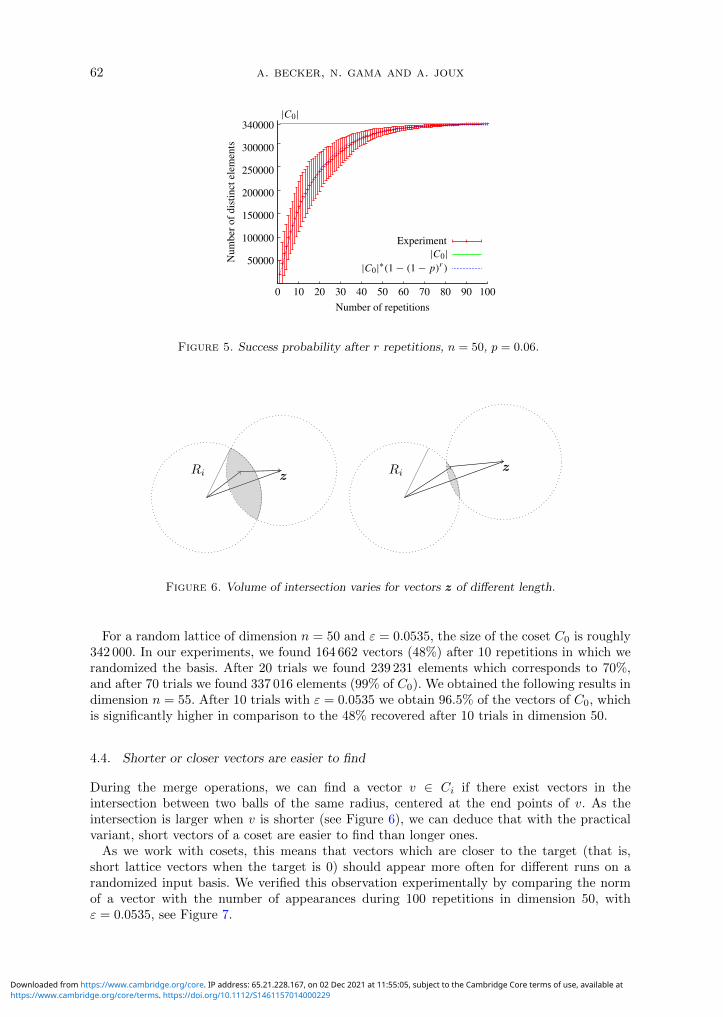
Figure 5. Success probability after r repetitions, n = 50, p = 0.06.

Ri z Ri z

Figure 6. Volume of intersection varies for vectors z of different length.

For a random lattice of dimension n = 50 and ε = 0.0535, the size of the coset C0 is roughly342 000. In our experiments, we found 164 662 vectors (48%) after 10 repetitions in which werandomized the basis. After 20 trials we found 239 231 elements which corresponds to 70%,and after 70 trials we found 337 016 elements (99% of C0). We obtained the following results indimension n = 55. After 10 trials with ε = 0.0535 we obtain 96.5% of the vectors of C0, whichis significantly higher in comparison to the 48% recovered after 10 trials in dimension 50.

4.4. Shorter or closer vectors are easier to find

During the merge operations, we can find a vector v ∈ Ci if there exist vectors in theintersection between two balls of the same radius, centered at the end points of v. As theintersection is larger when v is shorter (see Figure 6), we can deduce that with the practicalvariant, short vectors of a coset are easier to find than longer ones.

As we work with cosets, this means that vectors which are closer to the target (that is,short lattice vectors when the target is 0) should appear more often for different runs on arandomized input basis. We verified this observation experimentally by comparing the normof a vector with the number of appearances during 100 repetitions in dimension 50, withε = 0.0535, see Figure 7.



https://doi.org/10.1112/S1461157014000229



0

10

20

30

40

50

60

70

22 23 24 25 26 27 28 29 30 31

Occ

urre

nce

of v

ecto

r fo

r 10

0 ba

ses

Norm of the vector

Figure 7. Correlation of occurrence of vectors and their length.

4.5. Parallelization

The algorithm itself is highly parallelizable for various types of hardware architectures. Ofcourse, the dominant operations are n-dimensional vector additions and Euclidean normcomputations, which can be optimized on any hardware containing vector instructions.Additionally, unlike sieving techniques, each iteration of the outer for loop of the mergealgorithm (Algorithm 2, line 3) can be run simultaneously, as every vector is treatedindependently of the output. Furthermore, one may divide the pool of vectors into p 6 αn/2groups of buckets at each level, as soon as any two opposite buckets belong to the same group.Thus, the merge operation can operate on a group independently of all other groups. Thisallows us to efficiently run the algorithm when the available RAM is too small to store listsof size (1 + ε)nβn. It also allows us to distribute the merge step on a cluster. For instance,in dimension n = 90 using ε = 0.0416, storing the full lists would require 3 TB of RAM.We divided the lists into 25 groups of 120 GB each, which we treated one at a time in RAMwhile the others were kept on hard drive. This did not produce any noticeable slowdown.Finally, the number of elements in each bucket can be estimated precisely in advance usingHeuristic 2.1, and each group performs exactly the same vector operations (floating pointaddition, Euclidean norm computation) at the same time. This makes the algorithm suitablefor SIMD implementation, not only multi-threading.

4.6. Experiments in low- and middle-sized dimensions

Our experiments in dimension 40–90 on challenges in [35] show that we find the same shortvectors as those previously reported in the hall of fame. To solve SVP or CVP by use of thedecomposition technique, it is in fact not necessary to enumerate the complete bounded cosetC0 and to ensure that the lists are always of size (1 + εn)nβn as we describe in the followingparagraphs.

We give more details for medium dimensions n = 70 and n = 80 with α =√

4/3 and

β =√

3/2 in the following. The algorithm ran on a machine with an Opteron 6176 processor,containing 48 cores at 2.3 GHz, and having 256 GB of RAM. Table 2 presents the observedsize of the lists Si ⊆ Ci for each level in dimension 70 and 80.

In dimension 80, we chose aborted-BKZ-30 [17] for preprocessing. The algorithm has eightlevels and we chose ε = 0.044 to obtain 97% of C0 after a single run. The initial enumerationon one core took a very short time of 6.5 CPU hours (so less than 10 min with our multi-thread



https://doi.org/10.1112/S1461157014000229



implementation of the enumeration) while each of the eight levels of the merge took between20 and 36 CPU hours (so less than 45 min per level in our parallel implementation).

The number of elements in lower levels lies below the heuristic estimate and we keep loosingelements during the merge for the deepest levels. For example, in dimension 80 we start with73% of C8 and recover only 43% of C7 after one step. Towards higher levels, we slowly beginto recover more and more elements. In dimension 80, the size of the lists starts to increasefrom level 5 on as S5, S4 and S3 cover 41%, 47% and 56% of the vectors, respectively. Thiscontinues until the final step where we find 97% of the elements of C0.

4.7. Pruning of the merge step in practice, larger dimension n = 75 and n = 90

In § 3.1, we obtain conditions on the parameters as we request the intersection I of twoballs to be non-empty, which means that vol(I)/vol(L) > K for some number K > 1 underHeuristic 2.1. This condition suggests that at each level, each coset element in an output listSi−1 ⊆ Ci−1 of a merge is obtained on average about K times. If the input list Si is shorterthan expected, one will indeed recover fewer than K copies of each element, but we maystill have one representative of each element of Ci−1. Our experiments confirm this fact (seeTables 2 and 3). To solve SVP or CVP, one may shorten the time and memory necessary tofind a solution vector by interrupting each level whenever the output list contains a sufficientlylarge fraction of the elements of the bounded cosets. For example, we ran our algorithm onthe 75-dimensional basis of the SVP challenge [35] with seed 38. We chose ε = 0.044 andinterrupted the merge if the size of the intermediate set Si reached 50% or 35% of #Ci fori ∈ [1, k − 1]. Table 3 presents the intermediate list sizes. In the end, we recovered 69% and6.4% of #C0, respectively, and the shortest vector was found in both cases. The running timefor the merge in the intermediate levels decreases compared to no pruning by a factor 0.49and 0.29, respectively, as one would expect for lists that are smaller by at least a factor 0.5and 0.35, respectively.

In dimension 90, we ran our algorithm on the 90-dimensional SVP challenge with seed 11,using ε = 0.0416. We chose to keep at most 33% of Ci for i ∈ [1, k − 1]. Despite this harshcut, the size of the intermediate lists remained stable after the first merge. And interestingly,after only 65 h on 32 threads, we recovered 61% of #C0 in the end, including the publishedshortest vector. Note that as we interrupt the merge, we in fact do not read all elements ofthe starting list Sk. One might hence simply not apply a full enumeration in practice but stopthe Schnorr–Euchner enumeration once enough elements are enumerated.

4.8. Notes on the Gaussian heuristic for intermediate levels

Our quasi-orthogonal lattices at the bottom level behave randomly and follow the Gaussianheuristic. The most basic method to fill the bottom list Sk is to run Schnorr–Euchnerenumeration (see § 2) where the expected number of nodes in the enumeration tree is givenby (3.8) based on Heuristic 2.1. Previous research has established that this estimate is accurate

Table 2. Experimental results for n ∈ {70, 80}, α =√

4/3 and β =√

3/2.

Level = i 8 7 6 5 4 3 2 1 0

n = 80 #Si in millions 253 149 132 142 163 194 230 265 336

ε = 0.044 % of Gauss. heuristic 73 43 38 41 47 56 66 76 97

n = 70 #Si in millions – 38.8 20.3 19.0 20.0 20.3 23.1 26.5 29.8

ε = 0.049 % of Gauss. heuristic 95 50 46 50 56 65 73 87

n = 70 #Si in millions – 33.1 16.0 13.4 12.3 11.4 10.7 9.7 7

ε = 0.046 % of Gauss. heuristic 95 46 38 35 32 30.6 27.8 20



https://doi.org/10.1112/S1461157014000229



0

2e+06

4e+06

6e+06

8e+06

1e+07

1.2e+07

1.4e+07

0 10 20 30 40 50

Num

ber

of v

ecto

rs te

sted

Projection i = 1 to 55

ExperimentHeuristic

Figure 8. Comparison between the actual number of nodes during enumeration and the Gaussianheuristic predictions for dimension 55.

for random BKZ-reduced bases of random lattices in high dimension. Here, since we workwith quasi-orthogonal bases, which are very specific, we redo the experiments, and confirmthe findings also for quasi-orthogonal bases. Already for small dimensions (n = 40, 50, 55),experiments show that the actual number of nodes in a Schnorr–Euchner enumeration is veryclose to the expected value. Figure 8 shows that the experiment and heuristic estimate fordimension 55, for example, are almost indistinguishable.

We also make use of Heuristic 2.1 when we estimate the number of coset vectors in theintersection of two balls. As the lower lattices in the tower are not ‘random’ enough, theyhave close to quasi-orthonormal bases, we observe smaller lists in the lower levels and thusa deviation from the heuristic. Beside the geometry of lattices, the deviation depends onthe center of the balls or the center of the intersection. Randomly centered cosets of quasi-orthonormal lattices contain experimentally an average number of points a constant factorbelow (1 + εn)nβn. Zero-centered cosets contain more points, and should be avoided. Therandomization of the initial target used in Algorithm 1 ensures that the centers are randommodulo Lk, even in an SVP setting. The number of vectors hence stays below but close to theestimate (1 + εn)nβn after the first collision steps. The following steps can only improve thesituation. The lattices in higher levels are more and more random and we observe that thealgorithm recovers the expected number of vectors. This is a sign that our algorithm is stableeven when the input pools Si are incomplete.

Finally, experiments support the claim that the number of elements per bucket during themerge by collision corresponds to the average value (β/α)n. For example, in dimension n = 80,

Table 3. Experimental results with pruning, n ∈ {75, 80, 90}, α =√

4/3 and β =√

3/2.

Level = i 9 8 7 6 5 4 3 2 1 0 SVP

n = 75, % of Gauss. – – 50 50 47 46 46 48 50 69ε = 0.044 Heuris. Cut Cut Solvedn = 75, % of Gauss. – – 50 35 30 25 20 15 8 6.4ε = 0.044 Heuris. Cut Solvedn = 90, % of Gauss. 70 40 40 40 40 40 40 40 40 70ε = 0.0416 Heuris. Cut Cut Cut Cut Cut Cut Cut Cut Solvedn = 90, % of Gauss. 70 33 33 33 33 33 33 33 33 61ε = 0.0416 Heuris. Cut Cut Cut Cut Cut Cut Cut Cut Solved



https://doi.org/10.1112/S1461157014000229



for parameters α =√

4/3, β =√

3/2, ε = 0.044, we observe that the largest bucket containsonly 10% more elements than the average value, and that 60% of the buckets are within ±2%of the average value.

4.9. Comparison to experimental results of a parallel Gauss sieve algorithm

From a very general point of view, our algorithm can be viewed as a sieving algorithm. Thealgorithm is decomposed into a polynomial number of levels, each one corresponds to a certainupper bound Ri on the norm. At each level, we use an exponential pool of lattice vectors,perform linear combinations, and select the shortest of them for the next level.

We now list the specificities of our algorithm compared to previous sieving algorithms:

– We start from short vectors (in overlattices), and at each level the norm Ri geometricallyincreases by a factor α.

– At each level, we maintain an (almost) complete set of all coset vectors of norm less thanor equal to Ri. For this reason, our algorithm has the stability property that short cosetvectors are more likely to be found. Classical sieving techniques satisfy the opposite:short vectors have a negligible probability of appearing spontaneously. Our algorithm iscompatible with pruning, and it can solve the Exact CVP. Reducing the list sizes forclassical sieving leads in general to catastrophic results.

– Our algorithm is highly parallelizable as it allows us to use up to αn independent threadsper merge operation as explained in § 4.5. However, the accessible dimension is naturallylimited by the exponential memory requirement of order βn. There exists parallel versionsof the Gauss sieve [19, 29], which leads to faster practical running time in dimensions70 to 96, however the efficiency of the parallelization decreases fast when the number ofthreads increases because of the list size and the communication cost [19].

– Our algorithm is essentially a CVP solver and is not specialized for SVP: if classicalsieving algorithms were to be turned into CVP solvers, then it would obviously beimpossible to regroup each vector with its opposite, and the lists of vectors would be twiceas large. Furthermore, classical sieving techniques rely on the fact that vectors whichcannot be reduced by others, necessarily become poles to reduce others. By replacingsubtractions with additions in order to preserve the target, these two options, reducinga vector v by others and considering −v as a pole, cease to be mutually exclusive, andboth would have to be tested. Thus, turning classical sieving algorithms into CVP solverswould likely increase their running time by a factor of 4 and their memory requirementby a factor of 2, with no guarantee that they would actually find the solution.

We give some concrete timings. To solve instances in dimension 80 and 90, our algorithmtakes more time than the currently fastest implementation of the Gauss sieve algorithm [19].Ishiguro et al. report in [19] solving the SVP challenge in dimension 80 in 29 sequential hoursand an instance of dimension 96 in 6400 sequential hours. Our algorithm, however, needs 65sequential hours in dimension 80 and 2080 hours in dimension 90. It is slower than the Gausssieve used as an SVP solver, yet the slowdown factor remains smaller than 4, which would beexpected (as a minimum) to turn it into a CVP solver.

5. Conclusion

We have presented an alternative approach to solve the hard lattice problems SVP and CVPfor random lattices. It makes use of a new technique that is different from those used so far inenumeration or sieving algorithms, and works by moving short vectors along a tower of nestedlattices. Our experiments show that the method works well in practice. An open question inthe case of ideal lattices is to find a structural reduction that preserves the cyclic structure orprovides an other structure for which speed-ups can be applied.



https://doi.org/10.1112/S1461157014000229



Appendix A. Intersection of hyperballs

The volume of the intersection, volI(d), of two n-dimensional hyperballs of radius 1 at distanced ∈ [0.817; 2] can be approximated for large n by the volume of the n-dimensional ball of radius

D =√

1− (d/2)2 (see Lemma A.1 below). If we consider the intersection of two balls of radiusR, the volume gets multiplied by a factor of Rn, as stated in Corollary A.2.

Lemma A.1. The volume of the intersection of two n-dimensional hyperballs of radius 1 atdistance d ∈ [0.817; 2] is

2Vn−1

(n+ 1)Vnarccos

(d

2

)6

volI(d)

vol(Balln(D))6

2Vn−1

(n/2 + 1)Vnarccos

(d

2

)where D =

√1− (d/2)2.

Proof. The intersection of two balls of radius 1 whose centers are at distance d ∈ [0, 2] ofeach other can be expressed as

volI(d) = 2 ·∫1

d/2

Vn−1(√

1− x2)n−1 dx = 2Vn−1

∫arccos(d/2)

0

sinn(θ) dθ

where Vn−1 equals the volume of the (n − 1)-dimensional ball of radius 1. For d ∈ [0.817; 2]one can bound the sine term in the integral:

D

arccos(d/2)θ 6 sin(θ) 6

D√arccos(d/2)

√θ.

Therefore, we obtain bounds for the volume of the intersection,

volI(d) 62Vn−1

n/2 + 1arccos

(d

2

)Dn

and

volI(d) >2Vn−1

n+ 1arccos

(d

2

)Dn,

which proves the lemma.

We can use the lower bound of Lemma A.1 and obtain a numerical lower bound on the volumeof the intersection of balls of radius R at distance at most

√4/3R used in our algorithm:

Corollary A.2. For all dimensions n > 10, the volume of the intersection of two n-dimensional hyperballs of radius R at distance dR, where d 6

√4/3, is lower-bounded by

RnvolI(d) >0.692√n·Rnvol(Balln(

√1− (d/2)2)).

Appendix B. Proof of Theorem 3.2 and Algorithm B.1

We use the suffixes ‘old’ and ‘new’ to denote the values of the variables at the beginning andend of the ‘for’ loop of Algorithm B.1, respectively. Furthermore, we call xi the value ‖b∗new

i ‖during iteration i. Note that xi is also ‖b∗old

i ‖ during the next iteration (of index i− 1 since igoes backwards).

For i ∈ [1, n], let ai = ‖b∗i ‖/σ. Note that ai is always 1 or greater. We show by inductionover i that the following invariant holds at the end of each iteration of Algorithm B.1:



https://doi.org/10.1112/S1461157014000229



Algorithm B.1 Unbalanced reduction from [14], specialized for σ 6 min ‖b∗i ‖Input: An LLL-reduced basis B of an integer lattice L, and a target length σ 6 min ‖b∗i ‖Output: A basis C of L satisfying ‖c1‖ 6 σnvol(L)/σn, and, for all i ∈ [2, n], ‖c∗i ‖ 6 σ and

σn+1−i

vol(C[i,n])6 n+ 1− i.

1: C ← B2: Compute the Gram–Schmidt matrices µ and C∗

3: Let k be the largest index such that ‖c∗k‖ > σ4: for i = k − 1, . . . , 1 do

5: γ ←⌈−µi+1,i +

‖c∗i+1‖‖c∗

i ‖

√(‖c∗i ‖σ

)2 − 1⌉

6: (ci, ci+1)← (ci+1 + γ · ci, ci)7: Update the Gram–Schmidt matrices µ and C∗

8: end for9: return C

aixi+1 6 xi 6 aixi+1 + σai. (B.1)

At the first iteration (i = k − 1), it is clear that xk = ‖b∗oldk ‖ = σak. At the beginning of

iteration i, we always have ‖b∗oldi ‖ > σ, and by induction, ‖b∗old

i+1 ‖ > σ. We transform the blockso that the norm of the first vector satisfies

R 6 ‖b∗newi ‖ 6 R+ ‖b∗old

i ‖ (B.2)

where R = ‖b∗oldi+1 ‖‖b

∗oldi ‖/σ.

This condition can always be fulfilled with a primitive vector of the form bnewi = bold

i+1 + γboldi

for some γ ∈ Z. Since the volume is invariant, the new ‖b∗newi+1 ‖ is upper-bounded by σ.

And by construction, equation (B.2) is equivalent to the invariant (B.1) since ‖b∗oldi ‖ = aiσ,

‖b∗newi ‖ = xi and ‖b∗old

i+1 ‖ = xi+1.By developing (B.1), we derive a bound on x1,

x1 6 σ

k∑i=1

a1 . . . ai 6 σn

k∏i=1

ai 6 nσvol(L)/σn,

which proves (3.6). Similarly, one obtains that xi 6 (n + 1 − i)σ vol(B[i,n])/σn+1−i, which is

equivalent to (3.7). Note that the transformation matrix of the unbalanced reduction algorithmis

γ1 . . . γk−1 1 0 . . . 0

1 0 . . . 0...

...

0. . .

. . ....

......

0 0 1 0 0 . . . 0

0 . . . . . . 0 1 0 0...

... 0. . . 0

0 . . . . . . 0 0 0 1

where γi is d−µi+1,i + xi+1/σ

√1− 1/a2

i e. Since each xi+1 is bounded by



https://doi.org/10.1112/S1461157014000229



n∏j=i+1

aj =

n∏j=i+1

max(1, ||b∗j ||2/σ),

all coefficients have a size polynomial in the input basis. This proves that Algorithm B.1 haspolynomial running time.

References

1. M. Ajtai, ‘The shortest vector problem in L2 is NP-hard for randomized reductions (extended abstract)’,Proceedings of the 30th Annual ACM Symposium on Theory of Computing, STOC ’98 (ACM Press, 1998)10–19.

2. M. Ajtai, ‘Random lattices and a conjectured 0–1 law about their polynomial time computable properties’,Proceedings of the 43rd Symposium on Foundations of Computer Science, FOCS ’02 (IEEE ComputerSociety, 2002) 733–742.

3. M. Ajtai, R. Kumar and D. Sivakumar, ‘A sieve algorithm for the shortest lattice vector problem’,Proceedings of the 33rd Annual ACM Symposium on Theory of Computing, STOC ’01 (ACM Press,2001) 601–610.

4. A. Becker, J.-S. Coron and A. Joux, ‘Improved generic algorithms for hard knapsacks’, Advances incryptology — EUROCRYPT 2011, Lecture Notes in Computer Science 6632 (ed. K. G. Paterson; Springer,2011) 364–385.

5. A. Becker, A. Joux, A. May and A. Meurer, ‘Decoding random binary linear codes in 2n/20: how1 + 1 = 0 improves information set decoding’, Advances in cryptology — EUROCRYPT 2012, LectureNotes in Computer Science 7237 (ed. T. J. D. Pointcheval; Springer, 2012) 520–536.

6. M. I. Boguslavsky, ‘Radon transforms and packings’, Discrete Appl. Math. 111 (2001) no. 1–2, 3–22.7. X. Cade, D. Pujol and D. Stehle, fplll 4.0.4, May 2013.8. D. Coppersmith, ‘Finding a small root of a bivariate integer equation; factoring with high bits known’,

Advances in cryptology — EUROCRYPT 1996, Lecture Notes in Computer Science 1070 (ed. U. Maurer;Springer, 1996) 178–189.

9. D. Coppersmith, ‘Finding a small root of a univariate modular equation’, Advances in cryptology —EUROCRYPT 1996, Lecture Notes in Computer Science 1070 (ed. M. Darnell; Springer, 1996) 155–165.

10. I. Dinur, G. Kindler and S. Safra, ‘Approximating-CVP to within almost-polynomial factors is NP-hard’, Proceedings of the 39th Annual Symposium on Foundations of Computer Science, FOCS ’98 (IEEEComputer Society, 1998) 99.

11. T. G. et al., ‘GNU multiple precision arithmetic library 5.1.3’, September 2013, https://gmplib.org/.12. M. Fukase and K. Yamaguchi, ‘Finding a very short lattice vector in the extended search space’,

J. Information Processing 20 (2012) no. 3, 785–795.13. N. Gama, N. Howgrave-Graham, H. Koy and P. Q. Nguyen, ‘Rankin’s constant and blockwise lattice

reduction’, Advances in cryptology – CRYPTO 2006, Lecture Notes in Computer Science 4117 (Springer,2006) 112–130.

14. N. Gama, M. Izabachene, P. Q. Nguyen and X. Xie, ‘Structural lattice reduction: generalized worst-caseto average-case reductions’, Cryptology ePrint Archive, Report 2014/283, 2014.

15. N. Gama, P. Q. Nguyen and O. Regev, ‘Lattice enumeration using extreme pruning’, Advances incryptology — EUROCRYPT 2010, Lecture Notes in Computer Science 6110 (Springer, 2010) 257–278.

16. N. Gama, J. van de Pol and J. M. Schanck, ‘Fork of V. Shoup’s number theory library NTL, withimproved lattice functionalities’, February 2013, http://www.prism.uvsq.fr/∼gama/newntl.html.

17. G. Hanrot, X. Pujol and D. Stehle, ‘Analyzing blockwise lattice algorithms using dynamical systems’,Advances in cryptology — CRYPTO 2011, Lecture Notes in Computer Science 6841 (Springer, 2011)447–464.

18. G. Hanrot and D. Stehle, ‘Improved analysis of Kannan’s shortest lattice vector algorithm (extendedabstract)’, Advances in cryptology — CRYPTO 2007, Lecture Notes in Computer Science 4622 (Springer,2007) 170–186.

19. T. Ishiguro, S. Kiyomoto, Y. Miyake and T. Takagi, ‘Parallel Gauss sieve algorithm: solving the SVPin the ideal lattice of 128-dimensions’, Cryptology ePrint Archive, Report 2013/388, 2013.

20. A. Joux and J. Stern, ‘Lattice reduction: a toolbox for the cryptanalyst’, J. Cryptology 11 (1998) no. 3,161–185.

21. R. Kannan, ‘Improved algorithms for integer programming and related lattice problems’, Proceedings ofthe Fifteenth Annual ACM Symposium on Theory of Computing, STOC ’83 (ACM Press, 1983) 193–206.

22. R. M. Karp, ‘Reducibility among combinatorial problems’, Complexity of computer computations, IBMResearch Symposia Series (eds R. E. Miller and J. W. Thatcher; Plenum Press, New York, 1972) 85–103.

23. A. Korkine and G. Zolotarev, ‘Sur les formes quadratiques’, Math. Ann. 6 (1973) 336–389.24. A. K. Lenstra, H. W. Lenstra and L. Lovasz, ‘Factoring polynomials with rational coefficients’, Math.

Ann. 261 (1982) 515–534.


https://gmplib.org/

https://gmplib.org/

https://gmplib.org/

https://gmplib.org/

https://gmplib.org/

https://gmplib.org/

https://gmplib.org/

https://gmplib.org/

https://gmplib.org/

https://gmplib.org/

https://gmplib.org/

https://gmplib.org/

https://gmplib.org/

https://gmplib.org/

https://gmplib.org/

https://gmplib.org/

https://gmplib.org/

https://gmplib.org/

https://gmplib.org/

http://www.prism.uvsq.fr/~gama/newntl.html











































https://doi.org/10.1112/S1461157014000229



25. A. May, A. Meurer and E. Thomae, ‘Decoding random linear codes in 20.054n’, Advances in cryptology— ASIACRYPT 2011, Lecture Notes in Computer Science 7073 (Springer, 2011) 107–124.

26. D. Micciancio, ‘The shortest vector in a lattice is hard to approximate to within some constant’,Proceedings of the 39th Annual Symposium on Foundations of Computer Science, FOCS ’98 (IEEEComputer Society, 1998) 92.

27. D. Micciancio and P. Voulgaris, ‘A deterministic single exponential time algorithm for most latticeproblems based on Voronoi cell computations’, Proceedings of the 42nd ACM Symposium on Theory ofComputing, STOC ’10 (ACM Press, 2010) 351–358.

28. D. Micciancio and P. Voulgaris, ‘Faster exponential time algorithms for the shortest vector problem’,Proceedings of the Twenty-first Annual ACM–SIAM Symposium on Discrete Algorithms, SODA ’10(ACM/SIAM, 2010) 1468–1480.

29. B. Milde and M. Schneider, ‘A parallel implementation of gausssieve for the shortest vector problemin lattices’, Parallel computing technologies, Lecture Notes in Computer Science 6873 (Springer, 2011)452–458.

30. L. J. Mordell, ‘On some arithmetical results in the geometry of numbers’, Compos. Math. 1 (1935)248–253.

31. P. Q. Nguyen and T. Vidick, ‘Sieve algorithms for the shortest vector problem are practical’, J. Math.Cryptol. 2 (2008) no. 2, 181–207.

32. ‘OpenMP Architecture Review Board, OpenMP API version 4.0’, 2013.33. X. Pujol and D. Stehle, ‘Solving the shortest lattice vector problem in time 22.465n’, IACR Cryptology

ePrint Archive 2009/605, 2009.34. R. Rankin, ‘On positive definite quadratic forms’, J. Lond. Math. Soc. 28 (1953) 309–314.35. M. Schneider, N. Gama, P. Baumann and P. Nobach,

http://www.latticechallenge.org/svp-challenge/halloffame.php.36. K.-P. Schnorr and M. Euchner, ‘Lattice basis reduction: improved practical algorithms and solving

subset sum problems’, Math. Program. 66 (1994) 181–199.37. J. L. Thunder, ‘Higher-dimensional analogs of Hermite’s constant’, Michigan Math. J. 45 (1998) no. 2,

301–314.38. X. Wang, M. Liu, C. Tian and J. Bi, ‘Improved Nguyen–Vidick heuristic sieve algorithm for shortest

vector problem’, Proceedings of the 6th ACM Symposium on Information, Computer and CommunicationsSecurity, ASIACCS ’11 (ACM Press, 2011) 1–9.

39. F. Zhang, Y. Pan and G. Hu, ‘A three-level sieve algorithm for the shortest vector problem’, Selectedareas in cryptography — SAC 2013, Lecture Notes in Computer Science 8282 (eds T. Lange, K. Lauterand P. Lisonek; Springer, 2014).

Anja BeckerEPFL, Ecole Polytechnique Federale de

LausanneLaboratory for Cryptologic Algorithms

(LACAL)Switzerland

[email protected]

Nicolas GamaUVSQ/PRISMUniversite de VersaillesFrance

[email protected]

Antoine JouxCryptoExpertsINRIA/OuraganChaire de Cryptologie de la Fondation de

l’UPMCSorbonne UniversitesUPMC Univ Paris 06CNRS UMR 7606LIP 6France

[email protected]


http://www.latticechallenge.org/svp-challenge/halloffame.php





























































https://doi.org/10.1112/S1461157014000229


A sieve algorithm based on overlattices

Documents

Transcript of A sieve algorithm based on overlattices