- 1 -

A Scalable Method for Deductive Generalization in the Spreadsheet Paradigm1

Margaret Burnett*, Sherry Yang**, and Jay Summet* *Oregon State University **Oregon Institute of Technology Corvallis, Oregon Klamath Falls, Oregon {burnett, summet}@cs.orst.edu yangs@oit.edu

Abstract

In this paper, we present an efficient method for automatically generalizing programs written in spreadsheet languages. The strategy is to do generalization through incremental analysis of logical relationships among concrete program entities from the perspective of a particular computational goal. The method uses deductive dataflow analysis with algebraic back-substitution rather than inference with heuristics, and there is no need for generalization-related dialog with the user. We present the algorithms and their time complexities and show that, because the algorithms perform their analyses incrementally, on only the on-screen program elements rather than on the entire program, the method is scalable. Performance data is presented to help demonstrate the scalability.

1: INTRODUCTION

Like most researchers involved in end-user and graphical programming, we believe that concreteness, direct manipulation and immediate visual feedback are critical characteristics for end-user and graphical programming languages. These characteristics were first made widely available to end users in commercial spreadsheet systems, with great market success. Today, spreadsheet systems are the most widely-used type of end-user programming language. In this paper we present a new generalization method that supports extended use of these characteristics in the spreadsheet paradigm.

The spreadsheet paradigm includes not only commercial spreadsheet systems, but also a number of research languages that extend the paradigm with features such as gestural formula specification [Burnett and Gottfried 1998; Leopold and Ambler 1997], graphical types [Burnett and Gottfried 1998; Wilde and Lewis 1990], visual matrix manipulation [Ambler 1999; Wang and Ambler 1996], high-quality visualizations of complex data [Chi et al. 1998], and specifying GUIs [Myers 1991]. Forms/3 [Burnett and Gottfried 1998; Burnett et al. 2001a] is the extended spreadsheet language in which we have prototyped our method. Forms/3 can be described as a “gentle slope” language [Myers et al. 1992; Myers et al. 2000], intended to allow end users to create spreadsheets with fewer limitations than exist in other spreadsheet languages, while at the

1An early description of the approach described here appeared in [Yang and Burnett 1994].

- 2 -

same time allowing more sophisticated users with some programming background to create more powerful spreadsheets without having to leave the spreadsheet paradigm.

Our generalization method is compatible with traditional, single-grid spreadsheet languages, but also supports extended spreadsheet languages such as Forms/3 that relax several of the traditional restrictions. In solving the generalization problem in a way general enough to handle such extensions, we could not use the strictly spatial generalization approach based on physical relationships traditionally used by commercial spreadsheet systems. In these systems, when a user copies or “fills” a formula into other cells, the system generalizes any cell references in the copied formula based on the new cells’ number of rows and columns away from the original cell.

The commercial spreadsheet spatial approach fell short because, in the presence of features such as multiple grids and linked spreadsheet copies (such as multiple copies of a spreadsheet containing different data but mostly the same formulas), logical relationships—in addition to or instead of spatial relationships—must be used in defining the generalized meaning of the program. In considering alternatives to the spatial approach, we chose not to require the user to explicitly specify the intended generality in an abstract textual programming language, because such an approach would run counter to our goals of concrete programming via direct manipulation.

Many mechanisms to support automatic generalization of concrete programs have been devised for graphical programming languages [Ambler and Hsia 1993; Frank and Foley 1994; Kahn 1996; Kurlander and Feiner 1992; Lieberman 1993; McDaniel and Myers 1999; Myers 1993; Myers 1998; Olsen 1996; Perrone and Repenning 1998; Repenning 1995; Sassin 1994; Smith 1975; Sugiura and Koeski 1996; Vander Zanden and Myers 1995; Wolber 1997]. Some of these use inference1, and some require the user to explicitly provide the generalized meaning. The two most significant ways in which our method differs from these are:

• Neither inferential nor user-assisted: The generalization method presented in this paper

uses deductive analysis with algebraic substitution to derive a generalized program from a concrete one. Generalization is accomplished through the analysis of logical relationships among concrete program entities from the perspective of a particular computational goal. Because it does not use inference, there is no risk of “guessing wrong.”2 In contrast, other approaches to automatic generalization either use inference or require the user to provide additional information to the generalization mechanism.

• Scalable: The method presented here specifically addresses scalability. Scalability is necessary to maintain immediate visual feedback when programs increase in size. The method processes a program in a lazy, incremental fashion, operating only on the portion of the program currently on the screen. Thus, its cost is dependant upon display size, not upon overall program size. Prior generalization research has not investigated scalability properties of generalization methods.

In developing our method, we imposed three design constraints:

1 The convention in literature about demonstrational programming languages is that the term inference means reasoning techniques employing guesswork. For example, in the context of programming by demonstration, Myers and Maulsby define inferencing as the computer trying to determine the appropriate generalization using heuristics, which is in turn described as an alternative term for guessing [Myers and Maulsby 1993]. In this paper, we follow this convention. 2 Of course, the system cannot read the user’s mind. If the user enters incorrect relationships or enters a concrete program that does not fulfill their goals, then the generalized version will not fulfill their goals either.

- 3 -

• Orderlessness Constraint: The order in which a program is edited must not determine the final generalized form of the program. That is, if edits result in two concrete programs eventually becoming identical, then their generalizations must also be identical. This constraint is necessary to maintain the incremental, opportunistic, editing process that is usual in the spreadsheet paradigm.

• Modelessness Constraint: The method must not impose modes upon the user. By this we mean, there cannot be a “pre-generalization mode” that requires user actions or reasoning that are different from those of a “post-generalization mode.” Modelessness is one of the key characteristics of the spreadsheet paradigm that distinguishes it from traditional programming methods. Hence, it was critical to guard against loss of this characteristic.

• Generality Constraint: The method must be flexible enough to handle all non-circular cell referencing and linked spreadsheet “design patterns,” including patterns different from the call-return pattern of traditional programs, such as patterns resembling co-routines and pipelines. These patterns are possible in spreadsheets because of non-traditional scope and lifetime rules for its cells: every “variable” (cell) has global scope and persists until the program ends, and thus even intermediate cells can be referenced from any “procedure” (spreadsheet) at any time. The Generality Constraint honors this referencing flexibility.

We begin our presentation with a discussion of related work in Section 2, followed by an

introduction to the generalization method from the user’s perspective in Section 3. Section 4 explains in detail how the generalization method works behind the scenes, including the algorithms, their worst-case time costs, and the resulting scalability of the method. Section 5 extends the method to grids, temporal sequences and animations, and user-defined types. Performance measurements are given in Section 6, and then the paper concludes. For additional perspectives on the method’s correctness properties and costs, and for additional programming examples, see the supplementary information available from the ACM or the full technical report [Burnett et al. 2001b]. (Note to editor/ACM staff: these supplementary materials are temporarily included as appendices.)

2: RELATED WORK

The program entities that need to be generalized in a graphical or non-graphical spreadsheet language are the cell references. When a user enters a formula referencing some cell, that particular reference is not a problem, but when the formula is copied, replicated, or otherwise reused, its references need to be somehow generalized so that they will refer to cells appropriate for the new contexts.

For spreadsheet languages based upon a single grid, including commercial spreadsheet languages, generalization of cell references has been based strictly upon spatial relationships. However, this spatial strategy is limited—it works only for a single grid and, even with this restriction, it relies on inference heuristics that sometimes guess wrong. For example, if an Excel user inserts a new row just before a total row in a grid, the system automatically adjusts previous ranges used in the sums to exclude the row being added: that is, it infers that the user does not want to include the new row in the sums. (This is the correct inference if the user is adding a new subtotal row but is the incorrect inference if the user is adding a new detail row.) The method presented in this paper does not guess about spatial relationships; rather, it focuses primarily on logical relationships, and hence does not restrict a spreadsheet to any particular

- 4 -

number of grids—there can be multiple grids, and there can also be individual cells not part of any grid at all.

An earlier version of Forms/3 [Burnett and Ambler 1994] made a start at solving the generalization problem by contributing an internal textual notation to record the generality of a program, including its logical relationships in addition to its spatial relationships. However, no facility was present to deductively interpret a user’s direct manipulations in order to produce the notation. Also, although this internal notation was powerful enough to support the standard structures found in traditional programming languages such as subroutine-like relationships, it was not powerful enough to support non-traditional relationships.

Because of Forms/3’s extensive use of prototypical values for concreteness and direct manipulation, it shares with demonstrational languages some of the same difficulties in determining the generality intended by user-provided concrete prototypical values. Programming-by-demonstration systems solve the generalization problem in one of two ways: either (1) direct reliance on the user to explicitly provide generalization information, or (2) inference with user assistance and/or corrections. In both cases, the user assists the generalization process, by specifying which portions of their input should be generalized, by having to explicitly request generalization to achieve/maintain correctness, by selecting the most appropriate general form after the system has generated multiple possibilities, and/or by making corrections (e.g., via counter-examples) when the system has inferred an incorrect general program.

There are several ways a user can provide generalization information explicitly. For example, in Tinker [Lieberman 1993] the user explicitly provides the entire generalized meaning of a program. In PT [Ambler and Hsia 1993] the user explicitly differentiates between constants and generalized parameters. In ToonTalk [Kahn 1996] and in Topaz [Myers 1998], the user explicitly specifies the generalization parameters. In AgentSheets [Perrone and Repenning 1998; Repenning 1995] the user specifies any desired generalizations via analogies (“Cars move on roads like trains move on tracks”). In KidSim/Cocoa/Stagecast [Cypher and Smith 1995; Heger et al. 1998], users can generalize a graphical rule they have demonstrated by stating that it should abstract beyond the specific object type to, for example, all instances of a set of types.

Some programming-by-demonstration systems, such as Peridot [Myers 1993], Pavlov [Wolber 1997], and Gamut [McDaniel and Myers 1999], do not require as much explicit information from users and can rely on inference. This is possible because their limited problem domains (e.g., user interface construction, 2D board games) reduce the number of valid possibilities. Lapidary [Vander Zanden and Myers 1995], a one-way constraint demonstrational system for user interface construction, uses explicit user specification of some kinds of parameters but uses inference to generalize other kinds of parameters. Other inference-based approaches to generalization include inductive groups [Olsen 1996], in which the system generalizes properties of objects in a group explicitly selected by the user, and inferring the generalization of macros or functions from the user’s command history in applications such as in DemoOffice [Sugiura and Koeski 1996], ProDeGE+ [Sassin 1994], and Chimera [Kurlander and Feiner 1992].

Any inference technique can guess wrong, and systems based on inference therefore can generate incorrect programs if this possibility is not addressed. For example, Pavlov asks the user to constrain its inference via choices made through a dialog. When there is more than one possible generalization of a user’s history, DemoOffice uses a heuristic to choose the most likely, whereas ProDeGE+ and Chimera present the user with a dialog asking for clarification. One of the most advanced with respect to communicating about incorrect guesses is Gamut. When Gamut makes a mistake in generalization (either a failure to act or an inappropriate action) the

- 5 -

user corrects the system via “Stop That” and “Do Something” buttons. Because of this, in Gamut, the user assists the system only when it fails.

Forms/3’s generalization method is different from the methods described in this section in that Forms/3 does not use inference heuristics, and in Forms/3 the user does not need to explicitly request, assist, participate in, or correct the generalization process.

3: THE GENERALIZATION METHOD FROM THE USER’S PERSPECTIVE

3.1: Generalization Example: Population Visualization (User’s View)

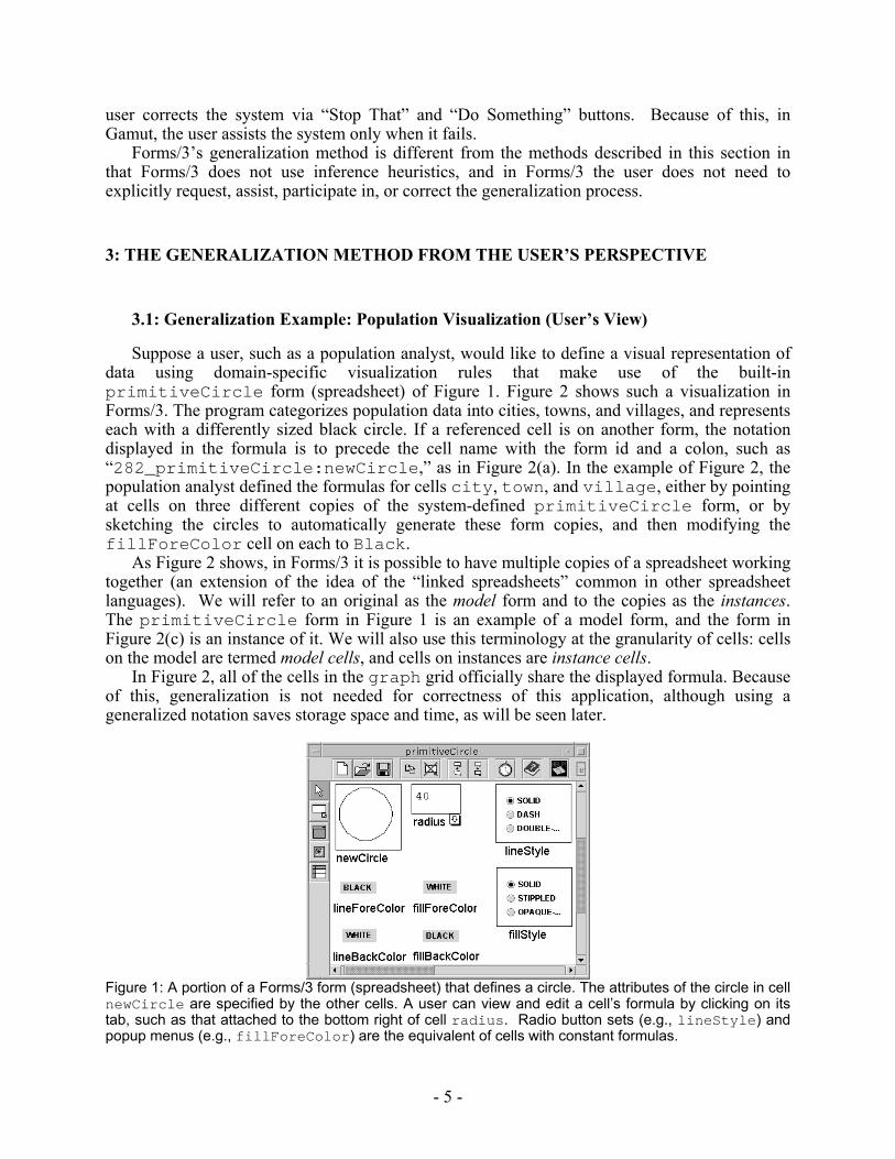
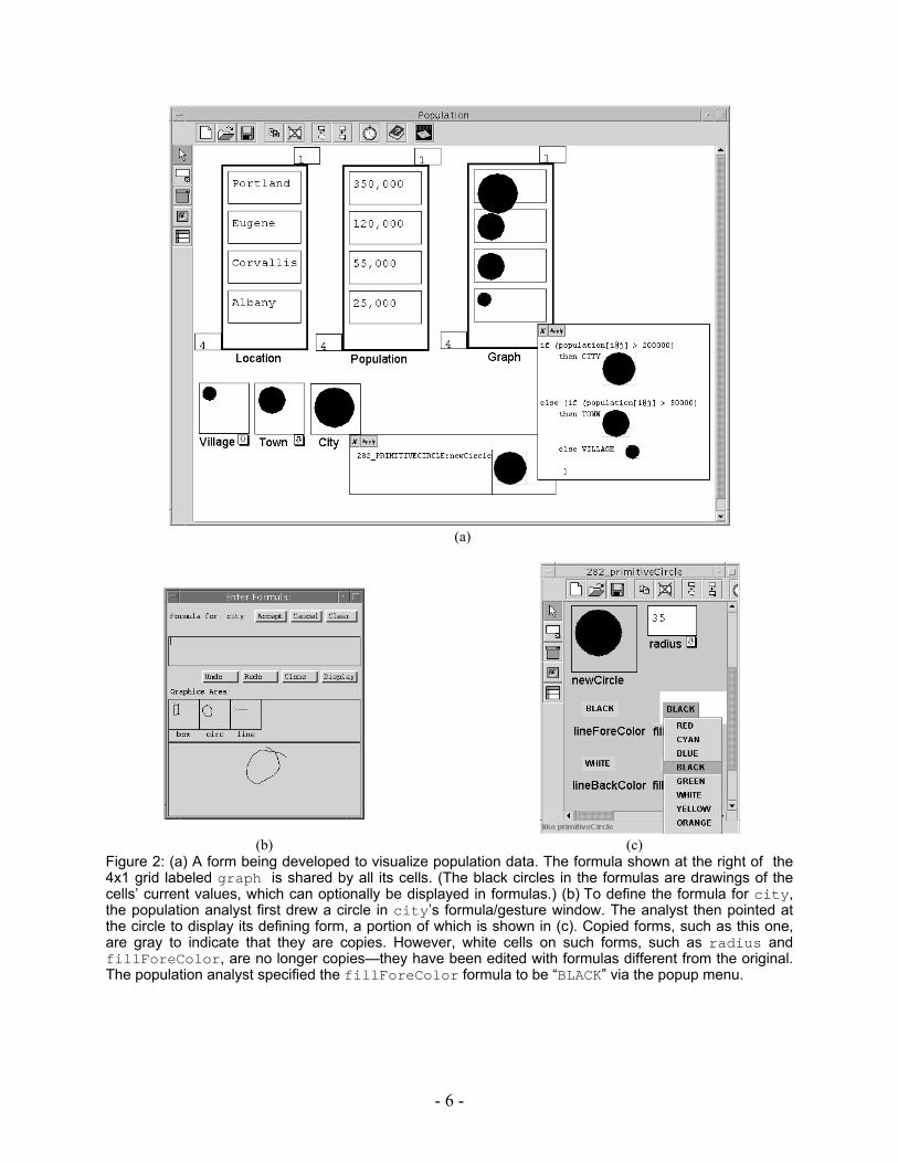
Suppose a user, such as a population analyst, would like to define a visual representation of data using domain-specific visualization rules that make use of the built-in primitiveCircle form (spreadsheet) of Figure 1. Figure 2 shows such a visualization in Forms/3. The program categorizes population data into cities, towns, and villages, and represents each with a differently sized black circle. If a referenced cell is on another form, the notation displayed in the formula is to precede the cell name with the form id and a colon, such as “282_primitiveCircle:newCircle,” as in Figure 2(a). In the example of Figure 2, the population analyst defined the formulas for cells city, town, and village, either by pointing at cells on three different copies of the system-defined primitiveCircle form, or by sketching the circles to automatically generate these form copies, and then modifying the fillForeColor cell on each to Black.

As Figure 2 shows, in Forms/3 it is possible to have multiple copies of a spreadsheet working together (an extension of the idea of the “linked spreadsheets” common in other spreadsheet languages). We will refer to an original as the model form and to the copies as the instances. The primitiveCircle form in Figure 1 is an example of a model form, and the form in Figure 2(c) is an instance of it. We will also use this terminology at the granularity of cells: cells on the model are termed model cells, and cells on instances are instance cells.

In Figure 2, all of the cells in the graph grid officially share the displayed formula. Because of this, generalization is not needed for correctness of this application, although using a generalized notation saves storage space and time, as will be seen later.

Figure 1: A portion of a Forms/3 form (spreadsheet) that defines a circle. The attributes of the circle in cell newCircle are specified by the other cells. A user can view and edit a cell’s formula by clicking on its tab, such as that attached to the bottom right of cell radius. Radio button sets (e.g., lineStyle) and popup menus (e.g., fillForeColor) are the equivalent of cells with constant formulas.

- 6 -

(a)

(b) (c)

Figure 2: (a) A form being developed to visualize population data. The formula shown at the right of the 4x1 grid labeled graph is shared by all its cells. (The black circles in the formulas are drawings of the cells’ current values, which can optionally be displayed in formulas.) (b) To define the formula for city, the population analyst first drew a circle in city’s formula/gesture window. The analyst then pointed at the circle to display its defining form, a portion of which is shown in (c). Copied forms, such as this one, are gray to indicate that they are copies. However, white cells on such forms, such as radius and fillForeColor, are no longer copies—they have been edited with formulas different from the original. The population analyst specified the fillForeColor formula to be “BLACK” via the popup menu.

- 7 -

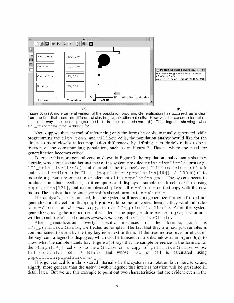
(a) (b)

Figure 3: (a) A more general version of the population program. Generalization has occurred, as is clear from the fact that there are different circles in graph’s different cells. However, the concrete formula—i.e., the way the user programmed it—is the one shown. (b) The legend showing what 179_primitiveCircle stands for.

Now suppose that, instead of referencing only the forms he or she manually generated while programming the city, town, and village cells, the population analyst would like for the circles to more closely reflect population differences, by defining each circle’s radius to be a fraction of the corresponding population, such as in Figure 3. This is where the need for generalization becomes critical.

To create this more general version shown in Figure 3, the population analyst again sketches a circle, which creates another instance of the system-provided primitiveCircle form (e.g., 179_primitiveCircle), and then edits the instance’s cell fillForeColor to Black and its cell radius to be “1 + (population:population[i@j] / 10000))” to indicate a generic reference to an element of the population grid. The system needs to produce immediate feedback, so it computes and displays a sample result cell radius using population[1@1], and recomputes/redisplays cell newCircle on that copy with the new radius. The analyst then refers in graph’s shared formula to newCircle.

The analyst’s task is finished, but the system still needs to generalize further. If it did not generalize, all the cells in the graph grid would be the same size, because they would all refer to newCircle on the same copy, such as 179_primitiveCircle. After the system generalizes, using the method described later in the paper, each reference in graph’s formula will be to cell newCircle on an appropriate copy of primitiveCircle.

After generalization, overly specific instances in the formula, such as 179_primitiveCircle, are treated as samples. The fact that they are now just samples is communicated to users by the tiny key icon next to them. If the user mouses over or clicks on the key icon, a legend is displayed, which can be transient or a subwindow as in Figure 3(b), to show what the sample stands for. Figure 3(b) says that the sample reference in the formula for the Graph[i@j] cells is to newCircle on a copy of primitiveCircle whose fillForeColor cell is Black and whose radius cell is calculated using population:population[i@j].

This generalized formula is stored internally by the system in a notation both more terse and slightly more general than the user-viewable legend; this internal notation will be presented in detail later. But we use this example to point out two characteristics that are evident even in the

- 8 -

legend viewable by the user: the generalized formula includes the name of the model form (namely, primitiveCircle) that was used to create the instance, and all the relevant cell relationships in which the instance differs from the model (namely, fillForeColor is Black, and radius is population:Graph[i@j]). These characteristics are needed so that the formula alone can provide enough information to enable the system (1) to find a form instance consistent with the generalized formula if such an instance exists, and (2) to create any needed form instance from its model form “just in time” at runtime, if such an instance does not already exist. Because of capability (1), if the user changes Albany’s population to 55,000, the system can look up a copy of primitiveCircle whose radius is 55,000 and whose fillForeColor is Black, which will allow it to reuse the Corvallis version for Albany. (This capability, a variant of lazy memoization [Hughes 1985], is important for efficiency, but is not necessary for correctness.) Because of capability (2), if the user makes the grids bigger and adds a new city with a population of 40,000, the system will be able to construct a copy of primitiveCircle with the appropriate cell formulas, even though the user never manually created this copy. This capability is necessary for correctness.

3.2: Generalization Example: Recursive Fibonacci (User’s View)

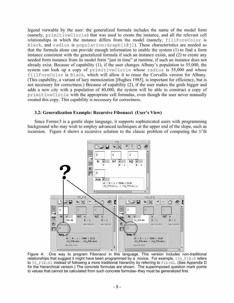
Since Forms/3 is a gentle slope language, it supports sophisticated users with programming background who may wish to employ advanced techniques at the upper end of the slope, such as recursion. Figure 4 shows a recursive solution to the classic problem of computing the N’th

Figure 4: One way to program Fibonacci in this language. This version includes non-traditional relationships that suggest it might have been programmed by a novice. For example, 104_FIB:N refers to 55_FIB:N1 instead of following a more traditional hierarchy by referring to Fib:N2. (See Appendix D for the hierarchical version.) The concrete formulas are shown. The superimposed question mark points to values that cannot be calculated from such concrete formulas–they must be generalized first.

- 9 -

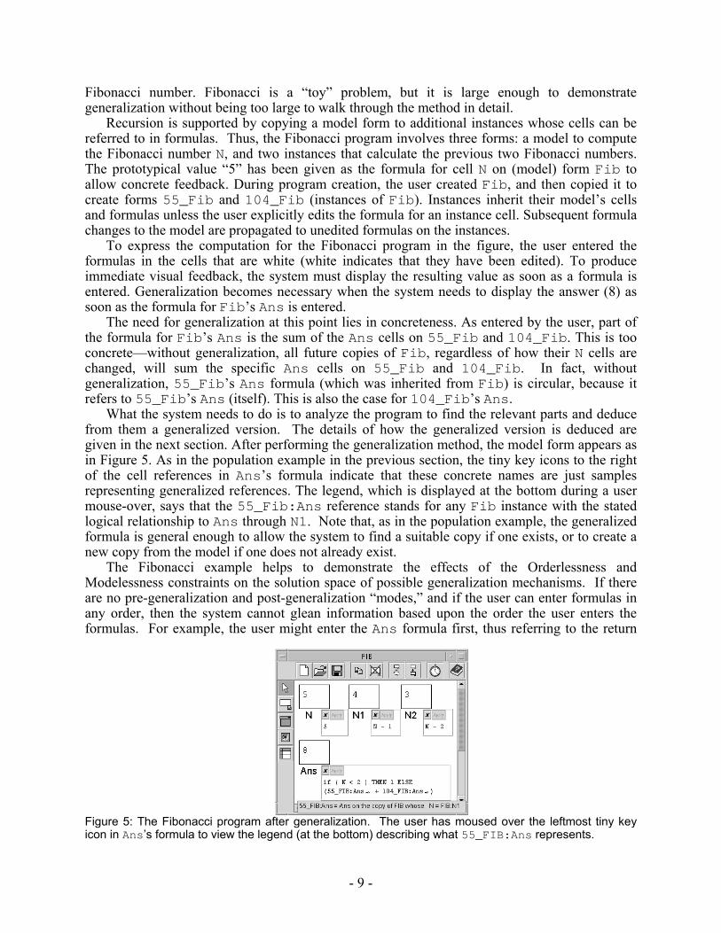
Fibonacci number. Fibonacci is a “toy” problem, but it is large enough to demonstrate generalization without being too large to walk through the method in detail.

Recursion is supported by copying a model form to additional instances whose cells can be referred to in formulas. Thus, the Fibonacci program involves three forms: a model to compute the Fibonacci number N, and two instances that calculate the previous two Fibonacci numbers. The prototypical value “5” has been given as the formula for cell N on (model) form Fib to allow concrete feedback. During program creation, the user created Fib, and then copied it to create forms 55_Fib and 104_Fib (instances of Fib). Instances inherit their model’s cells and formulas unless the user explicitly edits the formula for an instance cell. Subsequent formula changes to the model are propagated to unedited formulas on the instances.

To express the computation for the Fibonacci program in the figure, the user entered the formulas in the cells that are white (white indicates that they have been edited). To produce immediate visual feedback, the system must display the resulting value as soon as a formula is entered. Generalization becomes necessary when the system needs to display the answer (8) as soon as the formula for Fib’s Ans is entered.

The need for generalization at this point lies in concreteness. As entered by the user, part of the formula for Fib’s Ans is the sum of the Ans cells on 55_Fib and 104_Fib. This is too concrete—without generalization, all future copies of Fib, regardless of how their N cells are changed, will sum the specific Ans cells on 55_Fib and 104_Fib. In fact, without generalization, 55_Fib’s Ans formula (which was inherited from Fib) is circular, because it refers to 55_Fib’s Ans (itself). This is also the case for 104_Fib’s Ans.

What the system needs to do is to analyze the program to find the relevant parts and deduce from them a generalized version. The details of how the generalized version is deduced are given in the next section. After performing the generalization method, the model form appears as in Figure 5. As in the population example in the previous section, the tiny key icons to the right of the cell references in Ans’s formula indicate that these concrete names are just samples representing generalized references. The legend, which is displayed at the bottom during a user mouse-over, says that the 55_Fib:Ans reference stands for any Fib instance with the stated logical relationship to Ans through N1. Note that, as in the population example, the generalized formula is general enough to allow the system to find a suitable copy if one exists, or to create a new copy from the model if one does not already exist.

The Fibonacci example helps to demonstrate the effects of the Orderlessness and Modelessness constraints on the solution space of possible generalization mechanisms. If there are no pre-generalization and post-generalization “modes,” and if the user can enter formulas in any order, then the system cannot glean information based upon the order the user enters the formulas. For example, the user might enter the Ans formula first, thus referring to the return

Figure 5: The Fibonacci program after generalization. The user has moused over the leftmost tiny key icon in Ans’s formula to view the legend (at the bottom) describing what 55_FIB:Ans represents.

- 10 -

value Ans from 55_Fib before providing information that there will be an “input” cell N. Because no information about the N parameter-like cell is yet known, the reference to 55_Fib’s Ans at this point appears to be an absolute reference to a fixed cell (analogous to a reference to a global variable or constant in a traditional language), whereas instead it will be the result of a parameterized subroutine-like call when the user eventually enters the other formulas. For the user, this means freedom to work on the problem in any order that seems natural, but to the system it means lack of information.

The Generality constraint’s effects are also illustrated by the Fibonacci example. This program does not follow the traditional call-return pattern, because 104_Fib’s N is not defined in terms of Fib’s N2, but rather in terms of 55_Fib’s N1. Translated to traditional terms, Fib does not “call” 104_Fib, yet it refers directly to 104_Fib’s “return value.” Such patterns of references are not unusual in spreadsheet languages, and they make a program’s structure hard to predict because it will not always fall into traditional patterns.

4: BEHIND THE SCENES: THE GENERALIZATION ALGORITHMS

In the previous section, we showed how the generalization method looks to the user. Now we move behind the scenes to show the system’s view of generalization. In this section we describe generalization of single cells. Section 5 then describes the extensions that handle more complex structures, such as grids.

4.1: Overview

The method consists of two steps: 1) incrementally tracking logical relationships and 2) lazily generalizing these relationships “just in time.” In the Fibonacci example, step 1 consists of incrementally building a graph of the relationships among the N, N1, N2, and Ans cells on Fib, 55_Fib, and 104_Fib. This step is triggered whenever a user action establishes or changes a relationship. When the user enters the formula for Ans, step 2 is triggered because of the apparent circularity Ans introduces. Step 2 focuses on only those relationships necessary to compute Ans. Sometimes such relationships are complex and nested, so the system completes its work in a bottom-up fashion. Starting with some overly concrete cell reference, the system deduces a generalized description from the graph of relationships it built during step 1, and substitutes via algebraic back-substitution the generalized description into all relevant formulas that use the concrete reference. Generalization is complete when all the concrete instances involved in the computation being generalized (Ans, in this example) have finally been eliminated through these substitutions.

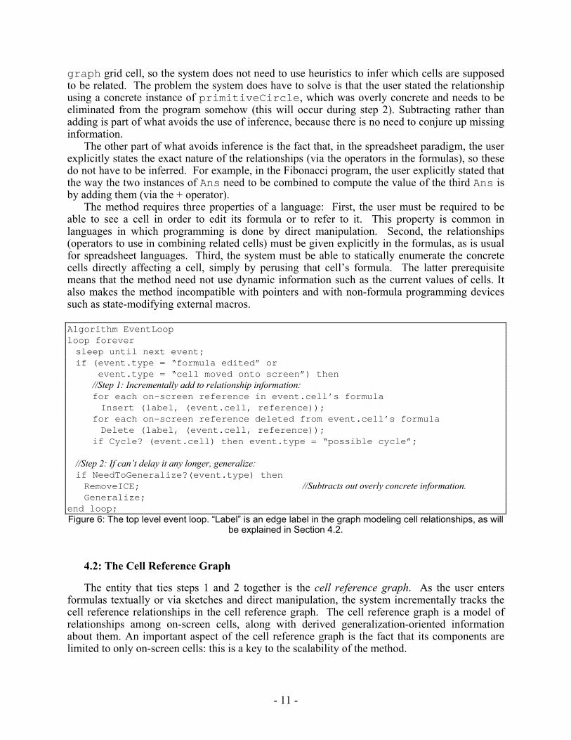
Driving the generalization method at the top level and deciding when it is time to take one of these steps is an event loop that watches for events relevant to generalization and calls the appropriate algorithms. See Figure 6. As is evident in the figure, the method is lazy and incremental.

As Figure 6 also shows, the method is subtractive. Most approaches to program generalization view the problem as being to generate missing information. However, our approach views the problem as being the presence of too much information, and removes extraneous, overly concrete information in order to arrive at the generalized version. (This view is shared by ToonTalk [Kahn 1996], although the way generalization is actually accomplished is quite different.) For example, in the population program, the user explicitly stated the relationship (via cell references) between a representative population grid cell, a radius cell on an instance of primitiveCircle, and the circle to be displayed for the corresponding

- 11 -

graph grid cell, so the system does not need to use heuristics to infer which cells are supposed to be related. The problem the system does have to solve is that the user stated the relationship using a concrete instance of primitiveCircle, which was overly concrete and needs to be eliminated from the program somehow (this will occur during step 2). Subtracting rather than adding is part of what avoids the use of inference, because there is no need to conjure up missing information.

The other part of what avoids inference is the fact that, in the spreadsheet paradigm, the user explicitly states the exact nature of the relationships (via the operators in the formulas), so these do not have to be inferred. For example, in the Fibonacci program, the user explicitly stated that the way the two instances of Ans need to be combined to compute the value of the third Ans is by adding them (via the + operator).

The method requires three properties of a language: First, the user must be required to be able to see a cell in order to edit its formula or to refer to it. This property is common in languages in which programming is done by direct manipulation. Second, the relationships (operators to use in combining related cells) must be given explicitly in the formulas, as is usual for spreadsheet languages. Third, the system must be able to statically enumerate the concrete cells directly affecting a cell, simply by perusing that cell’s formula. The latter prerequisite means that the method need not use dynamic information such as the current values of cells. It also makes the method incompatible with pointers and with non-formula programming devices such as state-modifying external macros.

Algorithm EventLooploop foreversleep until next event;if (event.type = “formula edited” or

event.type = “cell moved onto screen”) then//Step 1: Incrementally add to relationship information: for each on-screen reference in event.cell’s formulaInsert (label, (event.cell, reference));

for each on-screen reference deleted from event.cell’s formulaDelete (label, (event.cell, reference));

if Cycle? (event.cell) then event.type = “possible cycle”;

//Step 2: If can’t delay it any longer, generalize: if NeedToGeneralize?(event.type) thenRemoveICE; //Subtracts out overly concrete information.Generalize;

end loop;Figure 6: The top level event loop. “Label” is an edge label in the graph modeling cell relationships, as will

be explained in Section 4.2.

4.2: The Cell Reference Graph

The entity that ties steps 1 and 2 together is the cell reference graph. As the user enters formulas textually or via sketches and direct manipulation, the system incrementally tracks the cell reference relationships in the cell reference graph. The cell reference graph is a model of relationships among on-screen cells, along with derived generalization-oriented information about them. An important aspect of the cell reference graph is the fact that its components are limited to only on-screen cells: this is a key to the scalability of the method.

- 12 -

The cell reference graph CG = (V, LE) is a directed multi-graph of vertices V and labeled edges LE, where

V= {v | v is an on-screen cell in the program} LE = {(label(e),e) | label(e)∈ L and e∈ E} E = {(u,v) | cell u is referred to in v’s formula, where u, v ∈ V} L = {dg, dc, ig, ic} Although we refer to them as sets, LE and E are actually bags (sets allowing duplicates), as

are the subsets (sub-bags) of LE and E. An edge (u,v) in E is said to be direct if the user entered the reference to u in v’s formula,

whether by pointing at u, by typing its name explicitly into v’s formula, or by sketching/manipulating to generate a formula that explicitly references u. Edges that are not direct are inherited, and come about when the user copies a form, thereby causing cells on copied forms to inherit the same formulas as those on the original form. The terms concrete and generalized are used to describe a relationship’s current generalization state. Each relationship is modeled by an edge: an edge is said to be concrete if it has not yet been generalized; otherwise it is generalized. Because edges model cell relationships, we also map our terminology of edges to cell references and to the cells (nodes) in those relationships. For example, given a concrete edge (u,v), which models a reference u in v’s formula, we will refer to u as a concrete reference, and if v has concrete references in its formula then v is a concrete cell (node). We will employ this terminology mapping with the other terms describing edges as well: if (u,v) is a direct, generalized, or inherited edge, then u will be said to be a direct, generalized, or inherited reference, respectively, and so on.

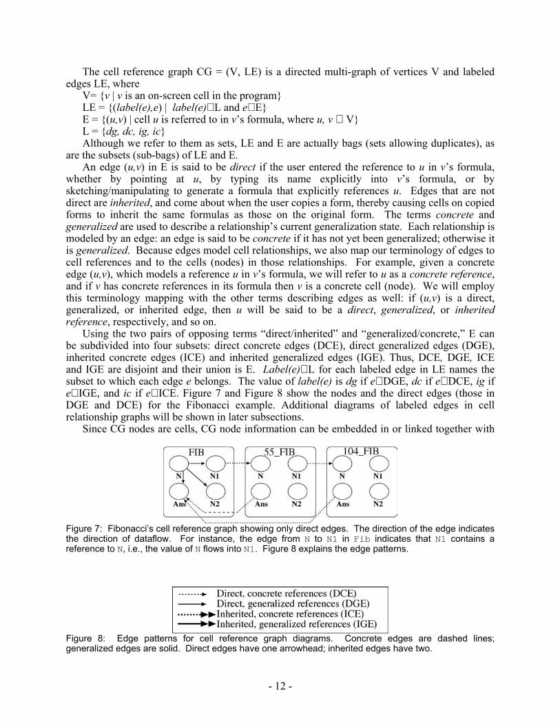
Using the two pairs of opposing terms “direct/inherited” and “generalized/concrete,” E can be subdivided into four subsets: direct concrete edges (DCE), direct generalized edges (DGE), inherited concrete edges (ICE) and inherited generalized edges (IGE). Thus, DCE, DGE, ICE and IGE are disjoint and their union is E. Label(e)∈ L for each labeled edge in LE names the subset to which each edge e belongs. The value of label(e) is dg if e∈ DGE, dc if e∈ DCE, ig if e∈ IGE, and ic if e∈ ICE. Figure 7 and Figure 8 show the nodes and the direct edges (those in DGE and DCE) for the Fibonacci example. Additional diagrams of labeled edges in cell relationship graphs will be shown in later subsections.

Since CG nodes are cells, CG node information can be embedded in or linked together with

Figure 7: Fibonacci’s cell reference graph showing only direct edges. The direction of the edge indicates the direction of dataflow. For instance, the edge from N to N1 in Fib indicates that N1 contains a reference to N, i.e., the value of N flows into N1. Figure 8 explains the edge patterns.

Figure 8: Edge patterns for cell reference graph diagrams. Concrete edges are dashed lines; generalized edges are solid. Direct edges have one arrowhead; inherited edges have two.

- 13 -

whatever data structure is already employed by the spreadsheet language for quick retrieval of cells. In our implementation, this is a hash table, where the hash key is the cell’s ID and the hash value is the cell.

In general, the following information is required for each node (cell) for generalization purposes:

General information about the cell, including (but not limited to) cellID, formula, and whether the cell is a model or an instance.

ModelCell: the model cell from which this cell was copied. (If this cell is itself a model cell, refers to itself.)

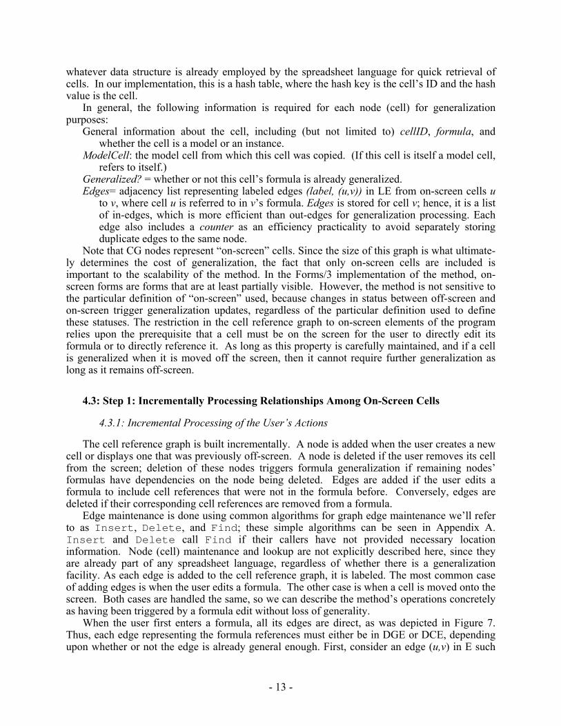
Generalized? = whether or not this cell’s formula is already generalized. Edges= adjacency list representing labeled edges (label, (u,v)) in LE from on-screen cells u

to v, where cell u is referred to in v’s formula. Edges is stored for cell v; hence, it is a list of in-edges, which is more efficient than out-edges for generalization processing. Each edge also includes a counter as an efficiency practicality to avoid separately storing duplicate edges to the same node.

Note that CG nodes represent “on-screen” cells. Since the size of this graph is what ultimate-ly determines the cost of generalization, the fact that only on-screen cells are included is important to the scalability of the method. In the Forms/3 implementation of the method, on-screen forms are forms that are at least partially visible. However, the method is not sensitive to the particular definition of “on-screen” used, because changes in status between off-screen and on-screen trigger generalization updates, regardless of the particular definition used to define these statuses. The restriction in the cell reference graph to on-screen elements of the program relies upon the prerequisite that a cell must be on the screen for the user to directly edit its formula or to directly reference it. As long as this property is carefully maintained, and if a cell is generalized when it is moved off the screen, then it cannot require further generalization as long as it remains off-screen.

4.3: Step 1: Incrementally Processing Relationships Among On-Screen Cells

4.3.1: Incremental Processing of the User’s Actions

The cell reference graph is built incrementally. A node is added when the user creates a new cell or displays one that was previously off-screen. A node is deleted if the user removes its cell from the screen; deletion of these nodes triggers formula generalization if remaining nodes’ formulas have dependencies on the node being deleted. Edges are added if the user edits a formula to include cell references that were not in the formula before. Conversely, edges are deleted if their corresponding cell references are removed from a formula.

Edge maintenance is done using common algorithms for graph edge maintenance we’ll refer to as Insert, Delete, and Find; these simple algorithms can be seen in Appendix A. Insert and Delete call Find if their callers have not provided necessary location information. Node (cell) maintenance and lookup are not explicitly described here, since they are already part of any spreadsheet language, regardless of whether there is a generalization facility. As each edge is added to the cell reference graph, it is labeled. The most common case of adding edges is when the user edits a formula. The other case is when a cell is moved onto the screen. Both cases are handled the same, so we can describe the method’s operations concretely as having been triggered by a formula edit without loss of generality.

When the user first enters a formula, all its edges are direct, as was depicted in Figure 7. Thus, each edge representing the formula references must either be in DGE or DCE, depending upon whether or not the edge is already general enough. First, consider an edge (u,v) in E such

- 14 -

that cells u and v are on the same form, as with the edge (Fib:N, Fib:N1) in Figure 7. The relationship about which copy of the Fib form is needed for N1’s reference to N is simple: the same copy for N as for N1. As this illustrates, edges among cells on the same form do not need further processing to become generalized, and the edge is an element of DGE. Edges that span multiple forms, such as (Fib:N1, 55_Fib:N) may need further processing, and they are elements of DCE.

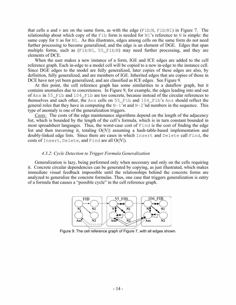
When the user makes a new instance of a form, IGE and ICE edges are added to the cell reference graph. Each in-edge to a model cell will be copied to a new in-edge to the instance cell. Since DGE edges to the model are fully generalized, later copies of these edges are also, by definition, fully generalized, and are members of IGE. Inherited edges that are copies of those in DCE have not yet been generalized, and are classified as ICE edges. See Figure 9.

At this point, the cell reference graph has some similarities to a dataflow graph, but it contains anomalies due to concreteness. In Figure 9, for example, the edges leading into and out of Ans in 55_Fib and 104_Fib are too concrete, because instead of the circular references to themselves and each other, the Ans cells on 55_Fib and 104_Fib’s Ans should reflect the general roles that they have in computing the N-1’st and N-2’nd numbers in the sequence. This type of anomaly is one of the generalization triggers.

Costs: The costs of the edge maintenance algorithms depend on the length of the adjacency list, which is bounded by the length of the cell’s formula, which is in turn constant bounded in most spreadsheet languages. Thus, the worst-case cost of Find is the cost of finding the edge list and then traversing it, totaling O(|V|) assuming a hash-table-based implementation and doubly-linked edge lists. Since there are cases in which Insert and Delete call Find, the costs of Insert, Delete, and Find are all O(|V|).

4.3.2: Cycle Detection to Trigger Formula Generalization

Generalization is lazy, being performed only when necessary and only on the cells requiring it. Concrete circular dependencies can be generated by copying, as just illustrated, which makes immediate visual feedback impossible until the relationships behind the concrete forms are analyzed to generalize the concrete formulas. Thus, one case that triggers generalization is entry of a formula that causes a “possible cycle” in the cell reference graph.

Figure 9: The cell reference graph of Figure 7, with all edges shown.

- 15 -

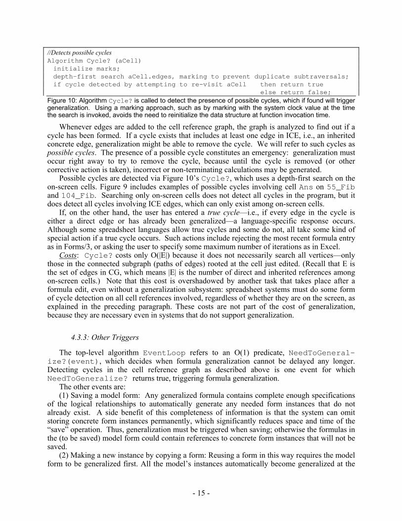
//Detects possible cycles Algorithm Cycle? (aCell)initialize marks;depth-first search aCell.edges, marking to prevent duplicate subtraversals;if cycle detected by attempting to re-visit aCell then return true

else return false;Figure 10: Algorithm Cycle? is called to detect the presence of possible cycles, which if found will trigger generalization. Using a marking approach, such as by marking with the system clock value at the time the search is invoked, avoids the need to reinitialize the data structure at function invocation time.

Whenever edges are added to the cell reference graph, the graph is analyzed to find out if a cycle has been formed. If a cycle exists that includes at least one edge in ICE, i.e., an inherited concrete edge, generalization might be able to remove the cycle. We will refer to such cycles as possible cycles. The presence of a possible cycle constitutes an emergency: generalization must occur right away to try to remove the cycle, because until the cycle is removed (or other corrective action is taken), incorrect or non-terminating calculations may be generated.

Possible cycles are detected via Figure 10’s Cycle?, which uses a depth-first search on the on-screen cells. Figure 9 includes examples of possible cycles involving cell Ans on 55_Fib and 104_Fib. Searching only on-screen cells does not detect all cycles in the program, but it does detect all cycles involving ICE edges, which can only exist among on-screen cells.

If, on the other hand, the user has entered a true cycle—i.e., if every edge in the cycle is either a direct edge or has already been generalized—a language-specific response occurs. Although some spreadsheet languages allow true cycles and some do not, all take some kind of special action if a true cycle occurs. Such actions include rejecting the most recent formula entry as in Forms/3, or asking the user to specify some maximum number of iterations as in Excel.

Costs: Cycle? costs only O(|E|) because it does not necessarily search all vertices—only those in the connected subgraph (paths of edges) rooted at the cell just edited. (Recall that E is the set of edges in CG, which means |E| is the number of direct and inherited references among on-screen cells.) Note that this cost is overshadowed by another task that takes place after a formula edit, even without a generalization subsystem: spreadsheet systems must do some form of cycle detection on all cell references involved, regardless of whether they are on the screen, as explained in the preceding paragraph. These costs are not part of the cost of generalization, because they are necessary even in systems that do not support generalization.

4.3.3: Other Triggers

The top-level algorithm EventLoop refers to an O(1) predicate, NeedToGeneral-ize?(event), which decides when formula generalization cannot be delayed any longer. Detecting cycles in the cell reference graph as described above is one event for which NeedToGeneralize? returns true, triggering formula generalization.

The other events are: (1) Saving a model form: Any generalized formula contains complete enough specifications

of the logical relationships to automatically generate any needed form instances that do not already exist. A side benefit of this completeness of information is that the system can omit storing concrete form instances permanently, which significantly reduces space and time of the “save” operation. Thus, generalization must be triggered when saving; otherwise the formulas in the (to be saved) model form could contain references to concrete form instances that will not be saved.

(2) Making a new instance by copying a form: Reusing a form in this way requires the model form to be generalized first. All the model’s instances automatically become generalized at the

- 16 -

same time, by virtue of their “copied” formulas—which are really just pointers to the model’s now-generalized formulas. If generalization did not happen at this point, the new instance could refer to an old instance that was too concrete to be appropriate for the new instance.

(3) Editing an instance cell that affects the generalized meaning of a previously generalized (on-screen) cell: As will become clear from the definition of the generalized notation in Section 4.4, this means the affected cell(s) must be re-generalized. This can only occur with on-screen cells, because of the next case. It is already necessary for spreadsheet evaluation engines, both lazy and eager, to do some updating of affected cells when an edit occurs [Burnett et al. 1998]; thus the only additional cost due to generalization is looking to see if those cells have been generalized.

(4) A form is removed from the screen: The departing form’s cells must be generalized and their cell reference dependencies removed from the cell reference graph. This is important to the method’s scalability because it keeps costs bounded by the number of on-screen cells, not by the number of cells in the program. (If the departing form is a model, its instances must depart too, to prevent later editing of the instances in a way that changes the generalized formulas of the off-screen cells.) Also, any on-screen cells that refer to the departing form’s cells must be generalized, before the departing cells are deleted from the cell reference graph.

These triggers help the approach to maintain an important invariant: all saved forms are generalized. For this reason, and because of the algebraic substitution basis of step 2, the outcome of generalization is independent of the order users edit or perform other operations that may trigger generalization—by the time a form is saved, it is guaranteed to be generalized, and the results will always be the same.

4.4: Step 2: Generalizing the Formula Relationships

Once formula generalization has been triggered, a subgraph of the cell reference graph is mapped to a compact textual notation. This notation is then processed to eliminate the concrete instances from the formula being generalized. This is done using algebraic back-substitution of relationships in place of concrete instances. The result is combined with the original formula to produce the generalized version of the formula. The details of these tasks are as follows.

4.4.1: The Subgraph of Interest

If the generalization trigger was one of those given in Section 4.3.3, then the entire cell reference graph is of interest. However, if the trigger was a formula edit generating a possible cycle, the cell containing the newly-edited formula can be viewed as the root of a smaller subgraph to be generalized, and only cells with paths to that root need be considered. We will refer to the subgraph of interest as SSCG (selected subgraph of CG).

Our method is subtractive: it removes edges from SSCG that are elements of ICE (inherited concrete edges), using the algorithm in Figure 11. The reason for removing ICE edges is that they are the ones that lead to anomalies such as those in the Fibonacci example. It is possible to remove them without losing important information because they are inherited: hence the same information can always be found in the original entry. In Figure 12, notice that only those cells relevant to the computation of the cell Ans are in SSCG. For example, the N2 cells are not present because there is no path in the cell reference graph from these cells to Ans.

Costs: Because the size of the CG is bounded by the number of cells on the screen, the size of SSCG, the subgraph being generalized, is also bounded by this number. Since RemoveICEedges walks through the triggering cells’ edge lists in depth-first order, the cost of RemoveICE is O(|E|) in the worst case. Marking is used to avoid duplicate visits. The call to

- 17 -

Delete is O(1) in this context, because the locations of the labeled edges passed to it have already been discovered.

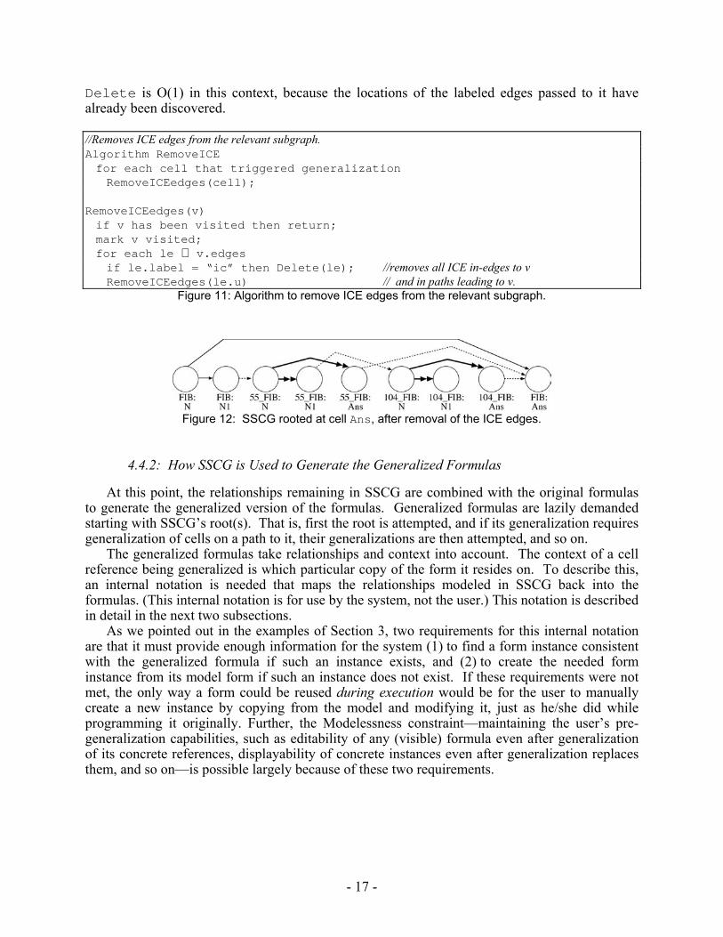
//Removes ICE edges from the relevant subgraph. Algorithm RemoveICEfor each cell that triggered generalizationRemoveICEedges(cell);

RemoveICEedges(v)if v has been visited then return;mark v visited;for each le ∈ v.edgesif le.label = “ic” then Delete(le); //removes all ICE in-edges to vRemoveICEedges(le.u) // and in paths leading to v.

Figure 11: Algorithm to remove ICE edges from the relevant subgraph.

Figure 12: SSCG rooted at cell Ans, after removal of the ICE edges.

4.4.2: How SSCG is Used to Generate the Generalized Formulas

At this point, the relationships remaining in SSCG are combined with the original formulas to generate the generalized version of the formulas. Generalized formulas are lazily demanded starting with SSCG’s root(s). That is, first the root is attempted, and if its generalization requires generalization of cells on a path to it, their generalizations are then attempted, and so on.

The generalized formulas take relationships and context into account. The context of a cell reference being generalized is which particular copy of the form it resides on. To describe this, an internal notation is needed that maps the relationships modeled in SSCG back into the formulas. (This internal notation is for use by the system, not the user.) This notation is described in detail in the next two subsections.

As we pointed out in the examples of Section 3, two requirements for this internal notation are that it must provide enough information for the system (1) to find a form instance consistent with the generalized formula if such an instance exists, and (2) to create the needed form instance from its model form if such an instance does not exist. If these requirements were not met, the only way a form could be reused during execution would be for the user to manually create a new instance by copying from the model and modifying it, just as he/she did while programming it originally. Further, the Modelessness constraint—maintaining the user’s pre-generalization capabilities, such as editability of any (visible) formula even after generalization of its concrete references, displayability of concrete instances even after generalization replaces them, and so on—is possible largely because of these two requirements.

- 18 -

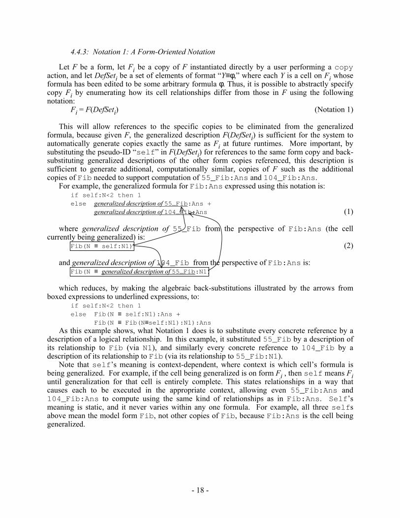
4.4.3: Notation 1: A Form-Oriented Notation

Let F be a form, let Fi be a copy of F instantiated directly by a user performing a copy action, and let DefSeti be a set of elements of format “Y≡φ,” where each Y is a cell on Fi whose formula has been edited to be some arbitrary formula φ. Thus, it is possible to abstractly specify copy Fi by enumerating how its cell relationships differ from those in F using the following notation: Fi = F(DefSeti) (Notation 1)

This will allow references to the specific copies to be eliminated from the generalized formula, because given F, the generalized description F(DefSeti) is sufficient for the system to automatically generate copies exactly the same as Fi at future runtimes. More important, by substituting the pseudo-ID “self” in F(DefSeti) for references to the same form copy and back-substituting generalized descriptions of the other form copies referenced, this description is sufficient to generate additional, computationally similar, copies of F such as the additional copies of Fib needed to support computation of 55_Fib:Ans and 104_Fib:Ans.

For example, the generalized formula for Fib:Ans expressed using this notation is: if self:N<2 then 1else generalized description of 55_Fib:Ans +

generalized description of 104_Fib:Ans (1)

where generalized description of 55_Fib from the perspective of Fib:Ans (the cell currently being generalized) is:

Fib(N ≡ self:N1) (2)

and generalized description of 104_Fib from the perspective of Fib:Ans is: Fib(N ≡ generalized description of 55_Fib:N1)

which reduces, by making the algebraic back-substitutions illustrated by the arrows from boxed expressions to underlined expressions, to:

if self:N<2 then 1else Fib(N ≡ self:N1):Ans +

Fib(N ≡ Fib(N≡self:N1):N1):Ans As this example shows, what Notation 1 does is to substitute every concrete reference by a

description of a logical relationship. In this example, it substituted 55_Fib by a description of its relationship to Fib (via N1), and similarly every concrete reference to 104_Fib by a description of its relationship to Fib (via its relationship to 55_Fib:N1).

Note that self’s meaning is context-dependent, where context is which cell’s formula is being generalized. For example, if the cell being generalized is on form Fi , then self means Fi until generalization for that cell is entirely complete. This states relationships in a way that causes each to be executed in the appropriate context, allowing even 55_Fib:Ans and 104_Fib:Ans to compute using the same kind of relationships as in Fib:Ans. Self’s meaning is static, and it never varies within any one formula. For example, all three selfs above mean the model form Fib, not other copies of Fib, because Fib:Ans is the cell being generalized.

- 19 -

4.4.4: Notation 2: Improving Notation 1 through Better Use of Granularity and Perspective

Because Notation 1 works at the granularity of forms, it suffices for supporting the traditional call-return hierarchical structure of one function invocation calling another, as found in traditional applicative languages, allowing even recursive programs to be programmed concretely and then generalized correctly. In fact, the above example even included a “pipeline” of values through the N cells, which the notation was also able to handle. If the technique were intended only for programmers, this amount of support might be adequate.

However, as the user sets up spreadsheets whose cells reference one another, he or she could introduce not only hierarchical and pipelined referencing patterns, but any arbitrary non-circular cell referencing pattern. Support for these other non-circular referencing patterns seems necessary as well, since it does not seem reasonable to expect end users to structure their programs in only the ways commonly used by professional programmers.

For example, suppose the first factor in Ans’s addition needed simply to be 1 more than the second factor. (To differentiate this changed version from the original example, at this point we now change the form names to NotFib.) One way to program this would be for the user to change 55_NotFib’s Ans cell’s formula to:

1 + 104_NotFib:Ans

Unfortunately, this change would prevent the formula for NotFib:Ans given in (1) above from being generalized as easily as before because, rather than (2), now the generalized description of 55_NotFib needs to include 104_NotFib’s generalized description:

NotFib(N ≡ self:N1,Ans ≡ 1 + generalized description of 104_NotFib:Ans) (3)

while 104_NotFib’s generalized description still needs to include 55_NotFib’s: NotFib(N ≡ generalized description of 55_NotFib:N1) (4)

One reason for the above apparent circularity comes from granularity: Notation 1 has been

describing relationships at the granularity of entire forms rather than cells. The other reason is that perspective has not been fully considered—which cell relationships are actually relevant in referring to some cell Z in a cell X’s formula.

Subgraph SSCG’s reduced membership to only cells relevant to the cell(s) being generalized, along with its topological ordering, provide ways to overcome both of these difficulties. Using SSCG, we change what is being described from forms (Notation 1) to cells, and make more use of perspective: only cells relevant to the cell X being described are included in X’s description. More precisely, every cell included on the left-hand side of a “≡” in a DefSeti in X’s formula must exist in SSCG and thus have a path to X.

If X is the cell whose formula is currently being generalized and its formula contains a concrete reference to Fi:Z, then let AffectsSetx be {Y≡φ | ∃ a path from Y to X in SSCG}, where φ is any formula. The strategy is to generalize X’s reference to Fi:Z using only cells that are in AffectsSetx, the set of Ys that directly or transitively affect X. Using this strategy, we modify the description of a generalized version of some concrete reference Fi:Z in X’s formula to be:

Fi:Z = F(DefSeti ∩ AffectsSetx):Z (Notation 2)

- 20 -

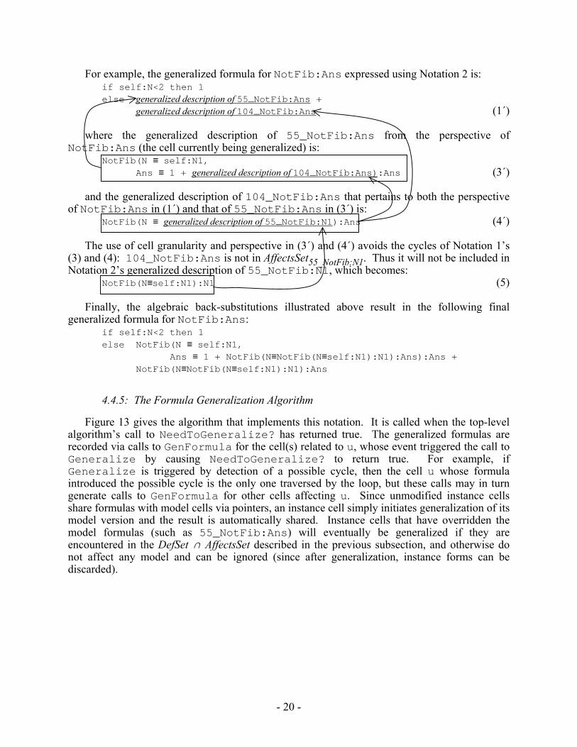
For example, the generalized formula for NotFib:Ans expressed using Notation 2 is: if self:N<2 then 1else generalized description of 55_NotFib:Ans +

generalized description of 104_NotFib:Ans (1´) where the generalized description of 55_NotFib:Ans from the perspective of

NotFib:Ans (the cell currently being generalized) is: NotFib(N ≡ self:N1,

Ans ≡ 1 + generalized description of 104_NotFib:Ans):Ans (3´)

and the generalized description of 104_NotFib:Ans that pertains to both the perspective of NotFib:Ans in (1´) and that of 55_NotFib:Ans in (3´) is:

NotFib(N ≡ generalized description of 55_NotFib:N1):Ans (4´) The use of cell granularity and perspective in (3´) and (4´) avoids the cycles of Notation 1’s

(3) and (4): 104_NotFib:Ans is not in AffectsSet55_NotFib:N1. Thus it will not be included in Notation 2’s generalized description of 55_NotFib:N1, which becomes:

NotFib(N≡self:N1):N1 (5) Finally, the algebraic back-substitutions illustrated above result in the following final

generalized formula for NotFib:Ans:if self:N<2 then 1else NotFib(N ≡ self:N1,

Ans ≡ 1 + NotFib(N≡NotFib(N≡self:N1):N1):Ans):Ans + NotFib(N≡NotFib(N≡self:N1):N1):Ans

4.4.5: The Formula Generalization Algorithm

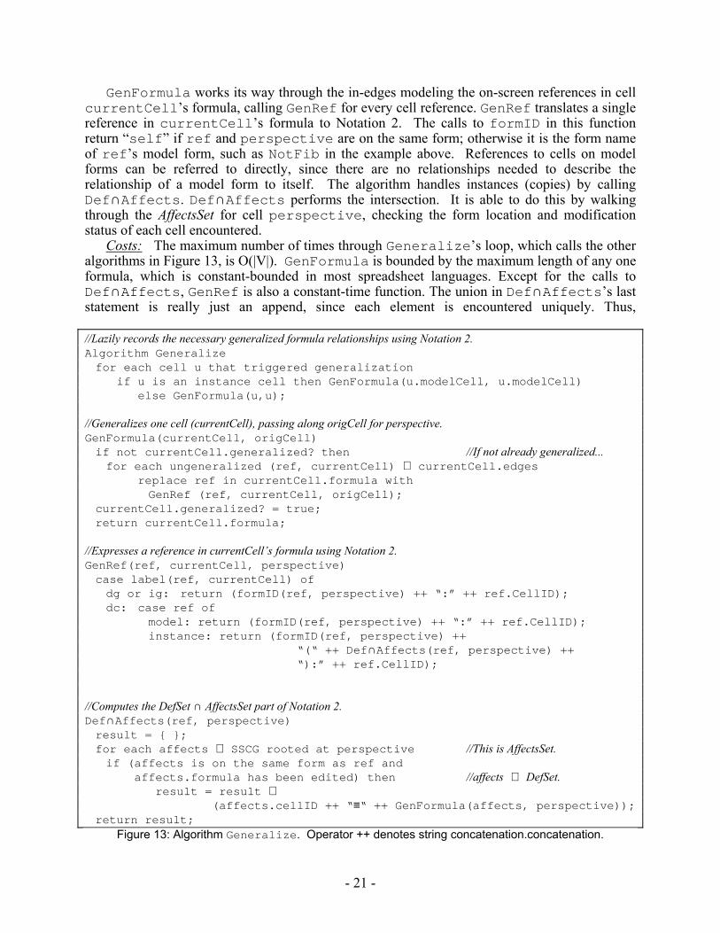
Figure 13 gives the algorithm that implements this notation. It is called when the top-level algorithm’s call to NeedToGeneralize? has returned true. The generalized formulas are recorded via calls to GenFormula for the cell(s) related to u, whose event triggered the call to Generalize by causing NeedToGeneralize? to return true. For example, if Generalize is triggered by detection of a possible cycle, then the cell u whose formula introduced the possible cycle is the only one traversed by the loop, but these calls may in turn generate calls to GenFormula for other cells affecting u. Since unmodified instance cells share formulas with model cells via pointers, an instance cell simply initiates generalization of its model version and the result is automatically shared. Instance cells that have overridden the model formulas (such as 55_NotFib:Ans) will eventually be generalized if they are encountered in the DefSet ∩ AffectsSet described in the previous subsection, and otherwise do not affect any model and can be ignored (since after generalization, instance forms can be discarded).

- 21 -

GenFormula works its way through the in-edges modeling the on-screen references in cell currentCell’s formula, calling GenRef for every cell reference. GenRef translates a single reference in currentCell’s formula to Notation 2. The calls to formID in this function return “self” if ref and perspective are on the same form; otherwise it is the form name of ref’s model form, such as NotFib in the example above. References to cells on model forms can be referred to directly, since there are no relationships needed to describe the relationship of a model form to itself. The algorithm handles instances (copies) by calling Def∩Affects. Def∩Affects performs the intersection. It is able to do this by walking through the AffectsSet for cell perspective, checking the form location and modification status of each cell encountered.

Costs: The maximum number of times through Generalize’s loop, which calls the other algorithms in Figure 13, is O(|V|). GenFormula is bounded by the maximum length of any one formula, which is constant-bounded in most spreadsheet languages. Except for the calls to Def∩Affects, GenRef is also a constant-time function. The union in Def∩Affects’s last statement is really just an append, since each element is encountered uniquely. Thus,

//Lazily records the necessary generalized formula relationships using Notation 2. Algorithm Generalizefor each cell u that triggered generalization

if u is an instance cell then GenFormula(u.modelCell, u.modelCell)else GenFormula(u,u);

//Generalizes one cell (currentCell), passing along origCell for perspective. GenFormula(currentCell, origCell)if not currentCell.generalized? then //If not already generalized...for each ungeneralized (ref, currentCell) ∈ currentCell.edges

replace ref in currentCell.formula withGenRef (ref, currentCell, origCell);

currentCell.generalized? = true;return currentCell.formula;

//Expresses a reference in currentCell’s formula using Notation 2. GenRef(ref, currentCell, perspective)case label(ref, currentCell) ofdg or ig: return (formID(ref, perspective) ++ “:” ++ ref.CellID);dc: case ref of

model: return (formID(ref, perspective) ++ “:” ++ ref.CellID);instance: return (formID(ref, perspective) ++

“(“ ++ Def∩Affects(ref, perspective) ++“):” ++ ref.CellID);

//Computes the DefSet ∩ AffectsSet part of Notation 2.Def∩Affects(ref, perspective)result = { };for each affects ∈ SSCG rooted at perspective //This is AffectsSet.if (affects is on the same form as ref and

affects.formula has been edited) then //affects ∈ DefSet.result = result ∪

(affects.cellID ++ “≡“ ++ GenFormula(affects, perspective));return result;

Figure 13: Algorithm Generalize. Operator ++ denotes string concatenation.concatenation.

- 22 -

Def∩Affects’s worst-case cost is dominated by the number of times through the loop, O(|E|). Multiplying these factors together gives a total for Generalize of O(|V|*|E|) if triggered

by a cell completing a possible cycle, or O(|V|2*|E|) if triggered by the other events such as removing a form from the screen. A further discussion of how the cost of this algorithm combines with the other algorithms when triggered by various user actions is provided in Appendix C. The most important aspect of the cost of this algorithm and the method’s other algorithms lies in the fact that they all depend on |V| and |E|, which are in turn bounded by the number of cells that fit on a screen—no matter how large the rest of the program is. (Appendix C contains a discussion of cost implications of different definitions of “on-screen.”) The method’s incremental strategy that allows the method to process only on-screen cells is the essence of the method’s scalability.

5: BEYOND SIMPLE CELLS

In this section we show how the generalization method can support more sophisticated spreadsheet entities than simple cells.

5.1: Grids

Arrays and matrices in traditional programming languages are ways to group data elements of similar attributes so that their elements can be processed using the same code. In a spreadsheet language, such grouping is done with grids, as in the population example shown earlier in Figure 3.

A grid has rows and columns. In Forms/3, grids are dynamically sized, and the number of rows and columns are determined dynamically by evaluating a distinguished cell for each, known as size cells. For example, Figure 3 shows the size cells for grid graph; formulas for these cells are entered in the usual way. The remaining cells in the grid (called the element cells) reside in regions. A region is a mechanism to define a shared formula for all the cells within a contiguous, rectangular group of cells1; for example, grid graph in Figure 3 consists of one region comprised of all the element cells in the grid. In Forms/3’s region formulas, i represents “my row” and j represents “my column.” At runtime, the evaluation engine substitutes a cell’s actual row and column location for the i and j in computing that particular cell’s value.

Since the region formulas make formula sharing explicit based on spatial relationships, it is not necessary to generalize further for that type of relationship. (Also, because the system does not need to adjust references (since they are already expressed generally), incorrect guesses such as the one triggered by the row insertion in Excel described in Section 2 do not arise.) However, in order to add the generality based on logical relationships shown earlier for simple cells, it is necessary to combine the generalization method presented earlier with the spatial relationship information already present in the shared formulas.

For example, recall from Section 3 that in the population example, the user began creating the formula for grid graph’s region in Figure 3 by drawing a circle then clicking on it to bring up an instance of the circle form, just as before in Figure 2. The user then brought up the instance of the circle form so as to specify two changes, changing the formula for fillForeColor to BLACK and the formula for radius to population[i@j], which says that eventually every element of the population grid is to be referred to in this way. To

1 Explicit sharing of this nature is also found in some other spreadsheet languages, such as Lotus and Formulate [Ambler 1999].

- 23 -

produce immediate feedback upon entry of this formula, the sample display value for radius is the grid element at row 1 column 1, which is population[1@1] in this example.

The entry of this formula triggers algorithm Generalize, which does the work of generalizing not only radius’s formula, but also the region formula in grid graph because of its dataflow relationship leading to radius. The resulting generalized region formula for the graph grid in Notation 2 becomes:

primitiveCircle( fillForeColor ≡ BLACK,radius ≡ 1 + population[i@j]/10000):newCircle

When processed by the evaluation engine, the contents of an element cell such as graph[3@1] will be computed as the result of cell newCircle in a copy of primitiveCircle in which fillForeColor’s formula is BLACK and radius’s formula refers to 1 + population[3@1]/10000.

5.1.1: Impacts on the Generalization Method

To add support for grids to the generalization method, the following straightforward additions were made to the algorithms of Section 4. First, there are new, implicit dependencies introduced by grids that needed to be maintained in the cell reference graph: the dependencies among the elements of a grid region, the grid’s size cells, and the grid as a whole. These dependencies are maintained in the cell reference graph automatically whenever a new formula is entered for a grid cell or region. These implicit dependencies are added to the cell reference graph as though they were explicit cell references made by the user (except that all cells in a region are represented by a single node in the graph to conserve space and time). As stated above, a new generalization trigger was added, which triggers generalization when an i@j grid subscript reference is entered by the user. Generalization is also triggered if a cell with an i@j grid subscript is present in the AffectsSet of a cell being edited. Finally, the front end of the system was made to use the sample display value of [1@1] when grid references are edited, i.e., prior to generalization. These were the only modifications needed, and they do not change the asymptotic cost of the algorithms; the cost still depends on the number of cells on the screen.

5.2: Animated Cell Values and the Time Dimension

Some graphical and end-user programming languages support temporal programming, the ability to explicitly define temporal relationships (e.g., [McDaniel and Myers 1999; Wolber 1997]). This is useful for graphical animations, for example. In spreadsheet languages, temporal programming and animation can be supported if formulas for cells are viewed as defining a vector of values along an explicit time dimension (a t-axis), rather than just an atomic value.

In Forms/3’s support of animation [Burnett et al. 2000], formulas can reference cells’ values at earlier moments in time. For example, on the circle form of Figure 1, cell radius’s formula could be changed so that, after an initial value at time 1, it refers to its own earlier value as in “radius<t-1> + 1” (adds 1 to the value of radius at t-position “now - 1”), which would cause newCircle to expand in size over time. In general, when cell A’s formula references cell B’s earlier value in time, where A and B are not necessarily distinct, a special temporal label is attached to the edge connecting B to A in the cell reference graph. The temporal label is needed to distinguish formulas referencing earlier values from truly circular references in the cycle detection routine. Without the temporal flag set, this apparent self-reference would have been falsely detected as a cycle. The temporal label is only used in the cycle detection routine. It does not otherwise change the generalization algorithms, and does not affect costs.

- 24 -

5.3: User-Defined Data Types

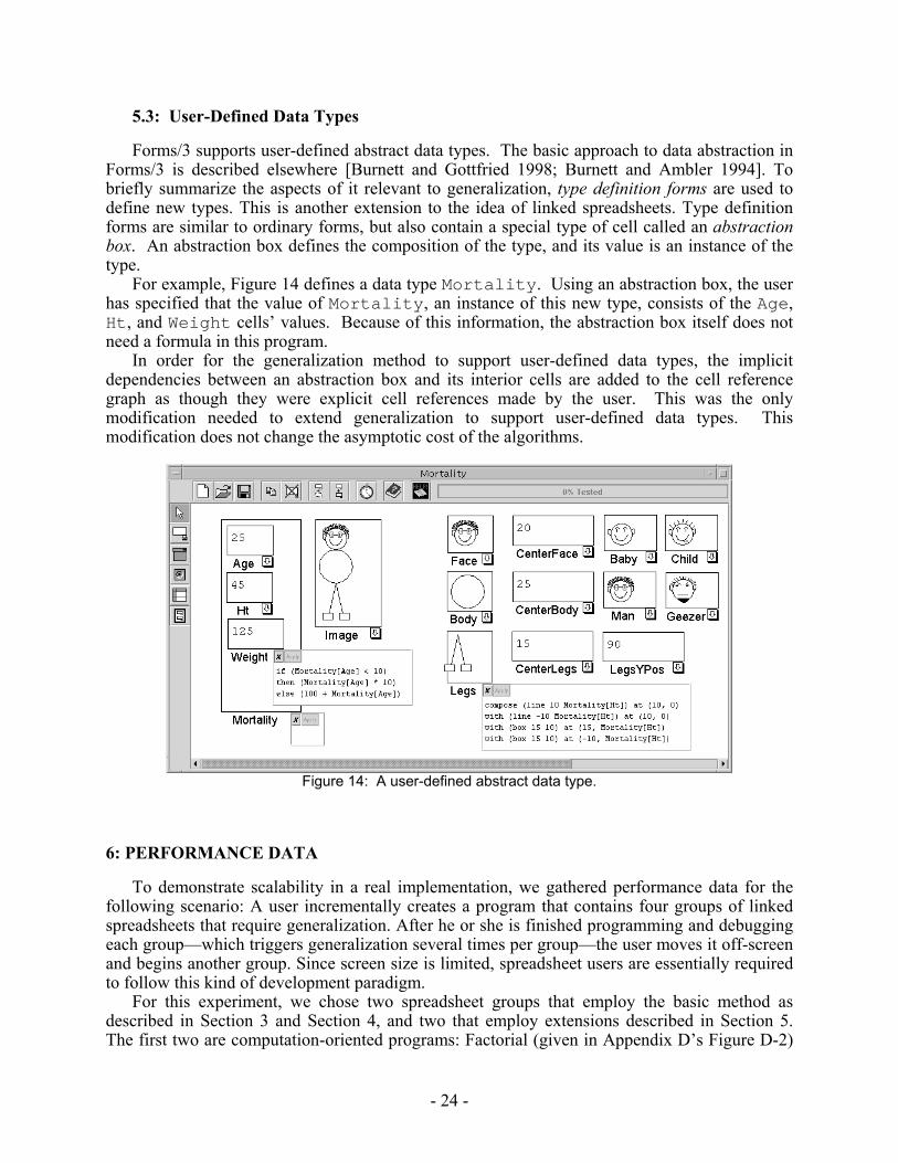
Forms/3 supports user-defined abstract data types. The basic approach to data abstraction in Forms/3 is described elsewhere [Burnett and Gottfried 1998; Burnett and Ambler 1994]. To briefly summarize the aspects of it relevant to generalization, type definition forms are used to define new types. This is another extension to the idea of linked spreadsheets. Type definition forms are similar to ordinary forms, but also contain a special type of cell called an abstraction box. An abstraction box defines the composition of the type, and its value is an instance of the type.

For example, Figure 14 defines a data type Mortality. Using an abstraction box, the user has specified that the value of Mortality, an instance of this new type, consists of the Age, Ht, and Weight cells’ values. Because of this information, the abstraction box itself does not need a formula in this program.

In order for the generalization method to support user-defined data types, the implicit dependencies between an abstraction box and its interior cells are added to the cell reference graph as though they were explicit cell references made by the user. This was the only modification needed to extend generalization to support user-defined data types. This modification does not change the asymptotic cost of the algorithms.

Figure 14: A user-defined abstract data type.

6: PERFORMANCE DATA

To demonstrate scalability in a real implementation, we gathered performance data for the following scenario: A user incrementally creates a program that contains four groups of linked spreadsheets that require generalization. After he or she is finished programming and debugging each group—which triggers generalization several times per group—the user moves it off-screen and begins another group. Since screen size is limited, spreadsheet users are essentially required to follow this kind of development paradigm.

For this experiment, we chose two spreadsheet groups that employ the basic method as described in Section 3 and Section 4, and two that employ extensions described in Section 5. The first two are computation-oriented programs: Factorial (given in Appendix D’s Figure D-2)

- 25 -

and the version of Fibonacci given in Appendix D’s Figure D-1. The third, Stock With Colors, is a business graphics program that makes use of the temporal extensions of Section 5, generating an animated bar chart of stock prices that are updated over time. It is given in Appendix D’s Figure D-3. The fourth, Population, is the visualization-oriented example of Figure 3, which employs the grid extensions described in Section 5.

We did all timings in a “lower-end” environment that does not have particularly optimal hardware or software. We used a single user Sun Ultra-1 (143Mhz CPU) under Solaris 8, using Lucid Common Lisp V5.0. Dynamic garbage collection was disabled to isolate its time, most of which is unrelated to the cost of the generalization algorithm. The combination of a relatively slow CPU and the Lisp computing environment falls at the lower end of the performance options available to today’s users, and is an acid test of the viability of our method in real-world computing environments.

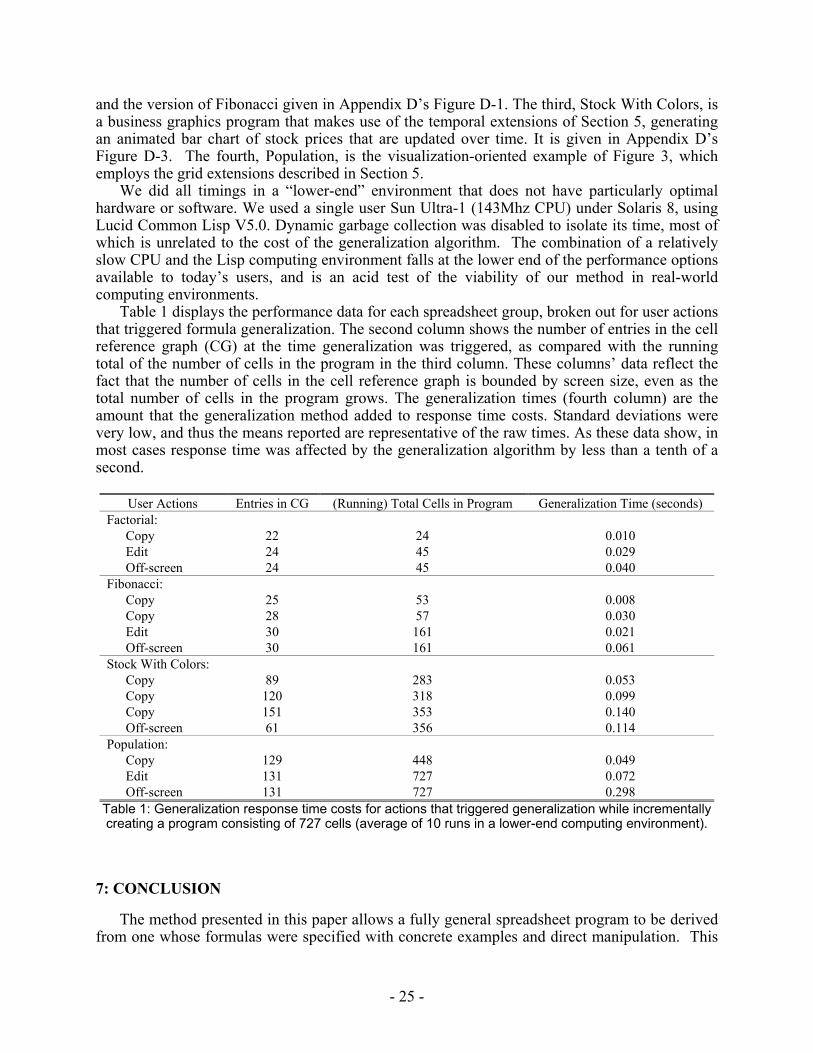
Table 1 displays the performance data for each spreadsheet group, broken out for user actions that triggered formula generalization. The second column shows the number of entries in the cell reference graph (CG) at the time generalization was triggered, as compared with the running total of the number of cells in the program in the third column. These columns’ data reflect the fact that the number of cells in the cell reference graph is bounded by screen size, even as the total number of cells in the program grows. The generalization times (fourth column) are the amount that the generalization method added to response time costs. Standard deviations were very low, and thus the means reported are representative of the raw times. As these data show, in most cases response time was affected by the generalization algorithm by less than a tenth of a second.

User Actions Entries in CG (Running) Total Cells in Program Generalization Time (seconds)

Factorial: Copy 22 24 0.010 Edit 24 45 0.029 Off-screen 24 45 0.040

Fibonacci: Copy 25 53 0.008 Copy 28 57 0.030 Edit 30 161 0.021 Off-screen 30 161 0.061

Stock With Colors: Copy 89 283 0.053 Copy 120 318 0.099 Copy 151 353 0.140 Off-screen 61 356 0.114

Population: Copy 129 448 0.049 Edit 131 727 0.072 Off-screen 131 727 0.298

Table 1: Generalization response time costs for actions that triggered generalization while incrementally creating a program consisting of 727 cells (average of 10 runs in a lower-end computing environment).

7: CONCLUSION

The method presented in this paper allows a fully general spreadsheet program to be derived from one whose formulas were specified with concrete examples and direct manipulation. This

- 26 -

is accomplished through recognizing and recording the logical relationships among the concrete data, from the perspective of the computational goals of the program fragment currently on the screen.

There are two primary contributions of this method. • It deductively reasons without the user having to provide generalization-oriented

information. Other generalization methods, whether deductive or inferential, have required user assistance either before generalization (such as to identify the differences between sample values and constants) or after generalization (to correct faulty inferences).

• It is the first generalization method to emphasize scalability. The costs of its generalization algorithms are bounded by the number of cells currently on the screen, not by the size of the program.

The combination of these two contributions with the design characteristics of orderlessness, modelessness, and generality lead to additional advantages. The combination of orderlessness and modelessness removes order requirements from the user’s programming process. The method is general in that all non-circular referencing patterns are supported, including those not commonly found in traditional programming languages. These characteristics allow the generalization method presented here to support a graphical style of spreadsheet programming that incorporates extensive use of concrete examples and direct manipulation, maintaining—even for large programs—the immediate visual feedback expected of spreadsheet environments.

ACKNOWLEDGMENTS

We thank the anonymous reviewers and the editor for their constructive feedback, which was very helpful in improving the quality of this paper. The population, mortality, and stocks examples were written by Herkimer Gottfried, Shikha Gottfried, and Miguel Arredondo-Castro. This work was supported in part by NSF awards CCR-9806821 and ITR-0082265, and by NASA grant NGT540022.

REFERENCES

[Ambler 1999] A. Ambler, “The Formulate Visual Programming Language,” Dr. Dobb’s Journal, 21-28, Aug. 1999.

[Ambler and Hsia 1993] A. Ambler and Y. Hsia, “Generalizing Selection in By-Demonstration Programming,” Journal of Visual Languages and Computing, 283-300, Sept. 1993.

[Burnett and Ambler 1994] M. Burnett and A. Ambler, “Interactive Visual Data Abstraction in a Declarative Visual Programming Language,” Journal of Visual Languages and Computing 5(1), 29-60, Mar. 1994.

[Burnett and Gottfried 1998] M. Burnett and H. Gottfried, “Graphical Definitions: Expanding Spreadsheet Languages through Direct Manipulation and Gestures,” ACM Transactions on Computer-Human Interaction 5(1), 1-33, Mar. 1998.

[Burnett et al. 1998] M. Burnett, J. Atwood, and Z. Welch, “Implementing Level 4 Liveness in Declarative Visual Programming Languages,” Proceedings of IEEE Symposium on Visual Languages, Halifax, Canada, 126-133, Sept. 1-4, 1998.

[Burnett et al. 2000] M. Burnett, N. Cao, and J. Atwood, “Time in Grid-Oriented VPLs: Just Another Dimension?” Proceedings of IEEE Symposium on Visual Languages, Seattle, WA, 137-144, Sept. 10-13, 2000.

[Burnett et al. 2001a] M. Burnett, J. Atwood, R. Djang, H. Gottfried, J. Reichwein, and S. Yang, “Forms/3: A First-Order Visual Language to Explore the Boundaries of the Spreadsheet Paradigm,” Journal of Functional Programming 11(2), 155-206, Mar. 2001.

[Burnett et al. 2001b] M. Burnett, S. Yang, and J. Summet, “A Scalable Method for Deductive Generalization in the Spreadsheet Paradigm,” TR 01-60-02, Oregon State University, January 2001.

- 27 -

[Chi et al. 1998] E. Chi, J. Riedl, P. Barry, and J. Konstan, “Principles for Information Visualization Spreadsheets,” IEEE Computer Graphics and Applications, July/Aug. 1998.

[Cypher and Smith 1995] A. Cypher and D. Smith, “KidSim: End User Programming of Simulations,” Proceedings of ACM Conference on Human Factors in Computing Systems, Denver, CO, 27-34, May 7-11, 1995.

[Frank and Foley 1994] M. Frank and J. Foley, “A Pure Reasoning Engine for Programming By Demonstration,” Proceedings of ACM Symposium on User Interface Software and Technology, Marina del Rey, CA, 95-101, Nov. 2-4, 1994.

[Heger et al. 1998] N. Heger, A. Cypher, and D. Smith, “Cocoa at the Visual Programming Challenge 1997,” Journal of Visual Languages and Computing 9(2), 151-169, Apr. 1998.

[Hughes 1985] J. Hughes, “Lazy Memo-Functions,” Proceedings of Functional Programming and Computer Architecture, Nancy, France, 129-146, Sept. 16-19, 1985. (Lecture Notes in Computer Science #201, J. Jouannaud, ed., Springer-Verlag).

[Kahn 1996] K. Kahn, “ToonTalk - An Animated Programming Environment for Children,” Journal of Visual Languages and Computing, 197-217, June 1996.

[Kurlander and Feiner 1992] D. Kurlander and S. Feiner, “A History-Based Macro by Example System,” Proceedings of ACM Symposium on User Interface Software and Technology, 99-106, 1992.

[Leopold and Ambler 1997] J. Leopold and A. Ambler, “Keyboardless Visual Programming Using Voice, Handwriting, and Gesture,” Proceedings of IEEE Symposium on Visual Languages, Capri, Italy, 28-35, Sept. 23-26, 1997.

[Lieberman 1993] H. Lieberman, “Tinker: A Programming by Demonstration System for Beginning Programmers,” in Watch What I Do: Programming by Demonstration (A. Cypher, ed.), MIT Press, Cambridge, MA, 48-64, 1993.

[McDaniel and Myers 1999] R. McDaniel and B. Myers, “Getting More Out of Programming By Demonstration,” Proceedings of ACM Conference on Human Factors in Computing Systems, Pittsburgh, PA, 442-449, May 15-20, 1999.

[Myers 1991] B. Myers, “Graphical Techniques in a Spreadsheet for Specifying User Interfaces,” Proceedings of ACM Conference on Human Factors in Computing Systems, New Orleans, LA, 243-249, Apr. 28 - May 2, 1991.

[Myers 1993] B. Myers, “Peridot: Creating User Interfaces by Demonstration,” in Watch What I Do: Programming by Demonstration (A. Cypher, ed.), MIT Press, Cambridge, MA, 124-153, 1993.

[Myers 1998] B. Myers, “Scripting Graphical Applications by Demonstration,” Proceedings of ACM Conference on Human Factors in Computing Systems, Los Angeles, 534-541, Apr. 18-23, 1998.

[Myers and Maulsby 1993] B. Myers and D. Maulsby, “Glossary,” in Watch What I Do: Programming by Demonstration (A. Cypher, ed.), MIT Press, Cambridge, MA, 593-603, 1993.

[Myers et al. 1992] B. Myers, D. Smith, and B. Horn, “Report of the ‘End-User Programming’ Working Group,” in Languages for Developing User Interfaces (B. Myers, ed.), A. K. Peters, Ltd., Wellesley, MA, 343-366, 1992.

[Myers et al. 2000] B. Myers, S. Hudson, and R. Pausch, “Past, Present, and Future of User Interface Software Tools,” ACM Transactions on Computer-Human Interaction 7(1), 3-28, Mar. 2000.

[Olsen 1996] D. Olsen Jr., “Inductive Groups,” Proceedings of ACM Symposium on User Interface Software and Technology, Seattle, WA, 193-199, Nov. 6-8, 1996.

[Perrone and Repenning 1998] C. Perrone and A. Repenning, “Graphical Rewrite Rule Analogies: Avoiding the Inherit or Copy & Paste Reuse Dilemma,” Proceedings of IEEE Symposium on Visual Languages, Halifax, Canada, 40-46, Sept. 1-4, 1998.

[Repenning 1995] A. Repenning, “Bending the Rules: Steps toward Semantically Enriched Graphical Rewrite Rules,” Proceedings of IEEE Symposium on Visual Languages, Darmstadt, Germany, 226-233, Sept. 5-9, 1995.

[Sassin 1994] M. Sassin, “Creating User-Intended Programs with Programming By Demonstration,” Proceedings of IEEE Symposium on Visual Languages, St. Louis, MO, 153-160, Oct. 4-7, 1994.

[Smith 1975] D. Smith, “Pygmalion: A Computer Program to Model and Stimulate Creative Thought,” Ph.D. Dissertation, Stanford University, 1975. (A more accessible summary of this work can be found in A. Cypher (ed.), Watch What I Do: Programming by Demonstration, MIT Press, Cambridge, MA, 1993.)

[Sugiura and Koseki 1996] A. Sugiura and Y. Koseki, “Simplifying Macro Definition in Programming By Demonstration,” Proceedings of ACM Symposium on User Interface Software and Technology, Seattle, WA, 173-182, Nov. 6-8, 1996.

[Vander Zanden and Myers 1995] B. Vander Zanden and B. Myers, “Demonstrational and Constraint-Based Techniques for Pictorially Specifying Application Objects and Behaviors,” ACM Transactions on Computer-Human Interaction 2(4), 308-356, Dec. 1995.

- 28 -

[Wang and Ambler 1996] G. Wang and A. Ambler, “Solving Display-Based Problems,” Proceedings of IEEE Symposium on Visual Languages, Boulder, CO, 122-129, Sept. 3-6, 1996.

[Wilde and Lewis 1990] N. Wilde and C. Lewis, “Spreadsheet-Based Interactive Graphics: From Prototype to Tool,” Proceedings of ACM Conference on Human Factors in Computing Systems, 153-159, Apr. 1990.

[Wolber 1997] D. Wolber, “An Interface Builder for Designing Animated Interfaces,” ACM Transactions on Computer-Human Interaction 4(4), 347-386, Dec. 1997.

[Yang and Burnett 1994] S. Yang and M. Burnett, “From Concrete Forms to Generalized Abstractions through Perspective-Oriented Analysis Of Logical Relationships,” Proceedings of IEEE Symposium on Visual Languages, St. Louis, MO, 6-14, Oct. 4-7, 1994.

- 29 -

Supplementary Material

Temporarily Included as

Appendices

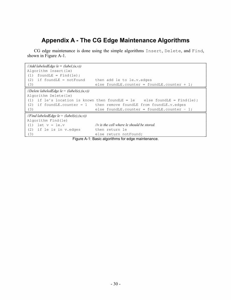
- 30 -

Appendix A - The CG Edge Maintenance Algorithms CG edge maintenance is done using the simple algorithms Insert, Delete, and Find,

shown in Figure A-1.

//Add labeledEdge le = (label,(u,v)) Algorithm Insert(le)(1) foundLE = Find(le);(2) if foundLE = notFound then add le to le.v.edges(3) else foundLE.counter = foundLE.counter + 1;

//Delete labeledEdge le = (label(e),(u,v)) Algorithm Delete(le)(1) if le’s location is known then foundLE = le else foundLE = Find(le);(2) if foundLE.counter = 1 then remove foundLE from foundLE.v.edges(3) else foundLE.counter = foundLE.counter - 1;

//Find labeledEdge le = (label(e),(u,v)) Algorithm Find(le)(1) let v = le.v //v is the cell where le should be stored.(2) if le is in v.edges then return le(3) else return notFound;

Figure A-1: Basic algorithms for edge maintenance.

- 31 -

Appendix B - Computational Equivalence Between Concrete and Generalized Formulas

We will say that the generalized version of a reference in cell X’s formula is computationally equivalent to the concrete version if replacing every concrete reference Fi:Z with the generalized reference results in the same value in cell X as with the concrete reference, provided that the concrete version terminates. In this section, we show that the generalization method maintains this property. The notion of computational equivalence is basically correctness of the method under the Modelessness constraint given in the introduction, which requires that there cannot be a “pre-generalization mode” that requires user actions or reasoning that are different from those of a “post-generalization mode.”

For now, assume the cell reference graph has information about all relationships in the program, i.e., that there are no off-screen cells, and that no ICE edges are present in the concrete version. (We will relax these assumptions in the next paragraph.) Under these assumptions, as we have pointed out before, replacing every reference Fi:Z with F(DefSeti):Z using Notation 1 would have maintained this property, since F(DefSeti) completely describes Fi by enumerating every difference between Fi and F. Despite its omission of information from Notation 1, Notation 2 does not lose this property, because a cell not in AffectsSetx cannot possibly have any effect on X’s value; hence a reference to Fi:Z = F(DefSeti ∩ AffectsSetx):Z must produce the same result in X as a reference to F(DefSeti):Z would produce. Hence the generalized version of the formula under both Notations 1 and 2 are computationally equivalent to the concrete version under these assumptions, provided that the concrete version terminates.

We now relax the above assumptions. First, we will allow some of the relationships in the program to be off-screen (and thus not in the cell reference graph). Because a trigger for generalizing is removal of a cell from the screen, we know that all relationships involving off-screen cells were generalized at the time the cell was removed. We have already explained that it is neither possible to change the relationships uniquely described in existing off-screen cells, nor to add new references to these off-screen cells without bringing them back onto the screen. Because of this property, all relationships involving an off-screen cell have already been generalized in a way that cannot be affected by the user’s manipulations and edits of on-screen information, and the cell reference graph can safely omit information about them. Even when off-screen cell formulas are generated via gestures, the generated formulas are created in pre-generalized form; after their creation the only way they can be edited in a way that requires new generalization activity is for them to be brought onto the screen.

Second, we will allow ICE edges to be present in the concrete version. Although these edges are removed from the cell reference graph, this does not result in loss of information, because the inherited references on form instances that these edges model are, by definition, simply duplicates of references that also exist in the model. Thus, the model form’s edges include the same information as the ICE edges and it is not necessary to include the latter’s duplicated information in order to generalize. It is also not necessary to actually generalize the inherited formulas modeled by the ICE edges, because cells with “inherited formulas” can just copy or use the formulas in the model version after generalization is complete.

Thus, the method satisfies the computational equivalence property for concrete forms that are able to terminate. We now consider concrete forms that do not terminate.

Concrete forms that do not terminate, due to possible cycles, are either incorrectly introducing true cycles, or are attempting to introduce recursion. Formulas introducing true

- 32 -

cycles are rejected, so no further attention to this situation is needed. For concrete forms attempting to introduce recursion, we now show that the “correct” recursive form is deduced, by induction on the number of recursive instances (references to other instances of the same form). By “correct,” we mean that the recursive form has the same relationships, except for the ICE edges, as those of the concrete forms.

The base case of the recursion (and also the base case of our induction)—references that do not refer to other instances of the same form—has already been demonstrated above. The inductive hypothesis is that n–1 recursive instances are correct. From this, it is obvious that the nth recursive instance is itself correct because it combines these instances using exactly the same operators as those specified concretely.

Finally, we show that generalization does not introduce infinite recursion if the concrete version did not do so. The key to this lies in the AffectsSet: the system does not include any cells in the generalized notation except those on the direct dataflow path to the formula being generalized, in essence following a lazy strategy. More generally, the system does not add any relationships that were not already specified by the user, and in fact eliminates all except those directly needed to compute the cell being generalized. Thus, since it does not add new relationships and eliminates those not needed for computation of the formula’s result, it cannot introduce infinite recursion if the concrete version did not do so.

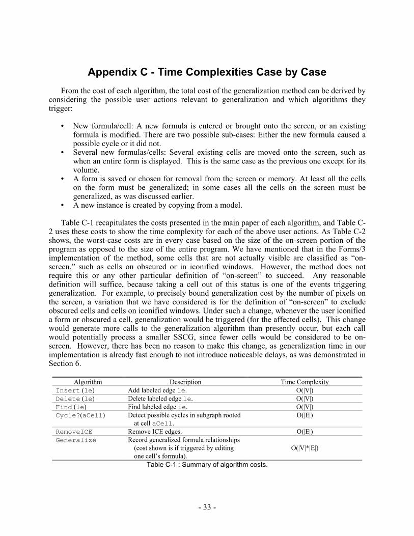
- 33 -

Appendix C - Time Complexities Case by Case From the cost of each algorithm, the total cost of the generalization method can be derived by

considering the possible user actions relevant to generalization and which algorithms they trigger:

• New formula/cell: A new formula is entered or brought onto the screen, or an existing

formula is modified. There are two possible sub-cases: Either the new formula caused a possible cycle or it did not.

• Several new formulas/cells: Several existing cells are moved onto the screen, such as when an entire form is displayed. This is the same case as the previous one except for its volume.

• A form is saved or chosen for removal from the screen or memory. At least all the cells on the form must be generalized; in some cases all the cells on the screen must be generalized, as was discussed earlier.

• A new instance is created by copying from a model. Table C-1 recapitulates the costs presented in the main paper of each algorithm, and Table C-

2 uses these costs to show the time complexity for each of the above user actions. As Table C-2 shows, the worst-case costs are in every case based on the size of the on-screen portion of the program as opposed to the size of the entire program. We have mentioned that in the Forms/3 implementation of the method, some cells that are not actually visible are classified as “on-screen,” such as cells on obscured or in iconified windows. However, the method does not require this or any other particular definition of “on-screen” to succeed. Any reasonable definition will suffice, because taking a cell out of this status is one of the events triggering generalization. For example, to precisely bound generalization cost by the number of pixels on the screen, a variation that we have considered is for the definition of “on-screen” to exclude obscured cells and cells on iconified windows. Under such a change, whenever the user iconified a form or obscured a cell, generalization would be triggered (for the affected cells). This change would generate more calls to the generalization algorithm than presently occur, but each call would potentially process a smaller SSCG, since fewer cells would be considered to be on-screen. However, there has been no reason to make this change, as generalization time in our implementation is already fast enough to not introduce noticeable delays, as was demonstrated in Section 6.

Algorithm Description Time Complexity

Insert (le) Add labeled edge le. O(|V|) Delete (le) Delete labeled edge le. O(|V|) Find (le) Find labeled edge le. O(|V|) Cycle?(aCell) Detect possible cycles in subgraph rooted

at cell aCell. O(|E|)

RemoveICE Remove ICE edges. O(|E|) Generalize Record generalized formula relationships

(cost shown is if triggered by editing one cell’s formula).

O(|V|*|E|)

Table C-1 : Summary of algorithm costs.

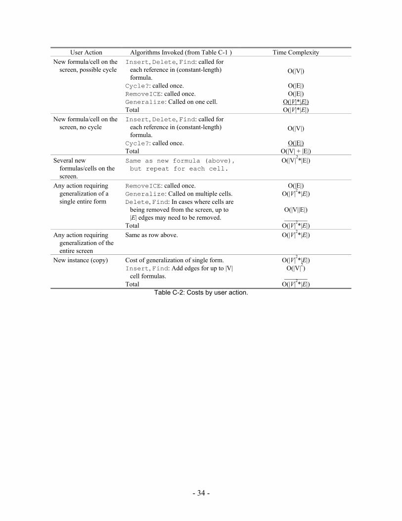
- 34 -

User Action Algorithms Invoked (from Table C-1 ) Time Complexity Insert, Delete, Find: called for

each reference in (constant-length) formula.

O(|V|)

Cycle?: called once. O(|E|) RemoveICE: called once. O(|E|) Generalize: Called on one cell. O(|V|*|E|)

New formula/cell on the screen, possible cycle

Total O(|V|*|E|) Insert, Delete, Find: called for

each reference in (constant-length) formula.

O(|V|)

Cycle?: called once. O(|E|)

New formula/cell on the screen, no cycle

Total O(|V| + |E|) Several new

formulas/cells on the screen.

Same as new formula (above),but repeat for each cell.

O(|V|2*|E|)

RemoveICE: called once. O(|E|) Generalize: Called on multiple cells. O(|V|2*|E|) Delete, Find: In cases where cells are

being removed from the screen, up to |E| edges may need to be removed.

O(|V||E|) _______

Any action requiring generalization of a single entire form

Total O(|V|2*|E|) Any action requiring

generalization of the entire screen

Same as row above. O(|V|2*|E|)

Cost of generalization of single form. O(|V|2*|E|) Insert, Find: Add edges for up to |V|

cell formulas. O(|V|2)

_______

New instance (copy)

Total O(|V|2*|E|) Table C-2: Costs by user action.

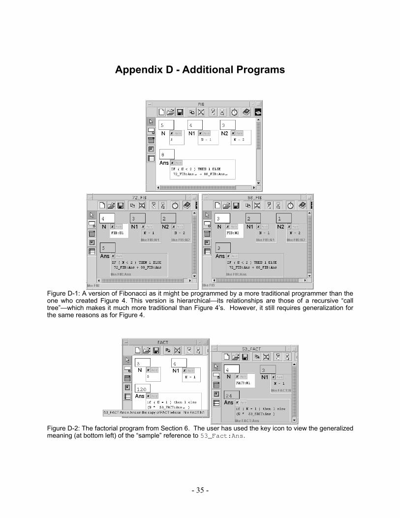
- 35 -

Appendix D - Additional Programs

Figure D-1: A version of Fibonacci as it might be programmed by a more traditional programmer than the one who created Figure 4. This version is hierarchical—its relationships are those of a recursive “call tree”—which makes it much more traditional than Figure 4’s. However, it still requires generalization for the same reasons as for Figure 4.

Figure D-2: The factorial program from Section 6. The user has used the key icon to view the generalized meaning (at bottom left) of the “sample” reference to 53_Fact:Ans.

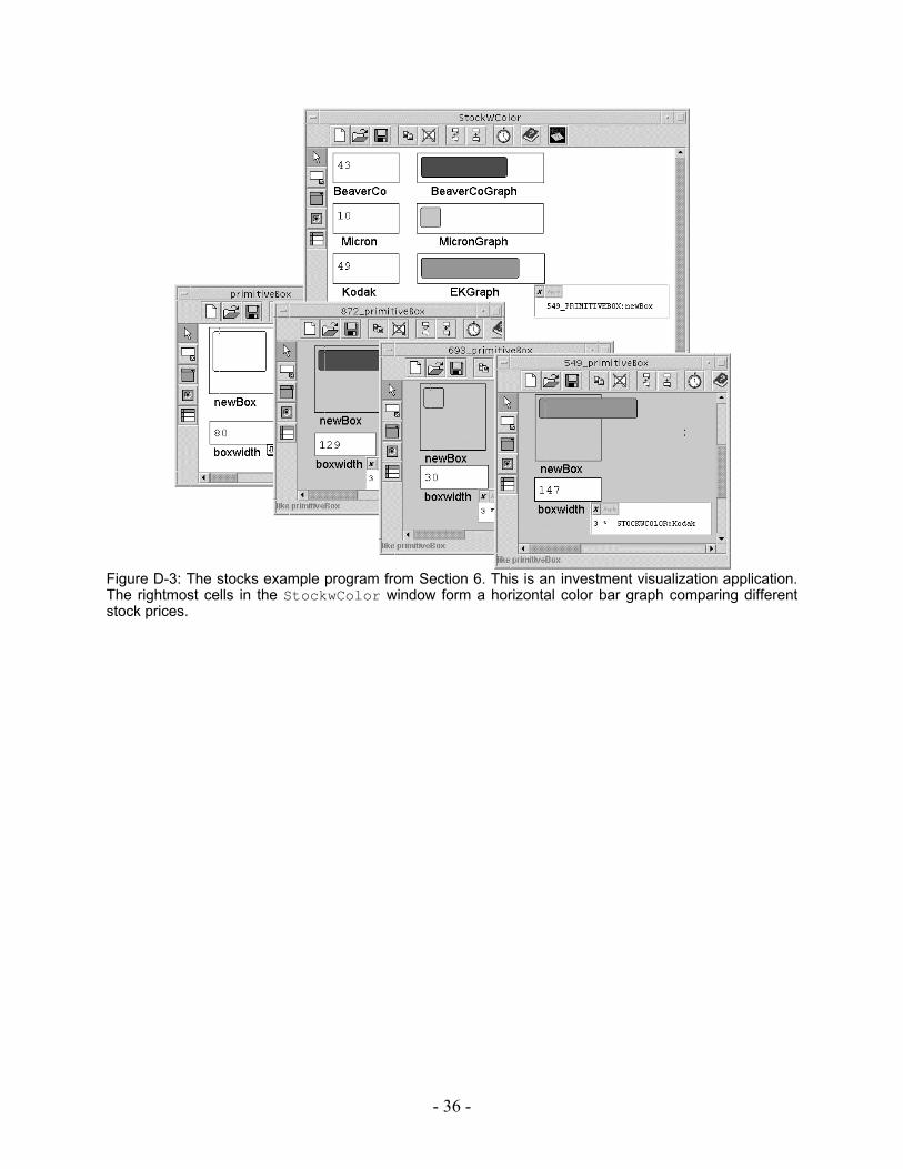
- 36 -

Figure D-3: The stocks example program from Section 6. This is an investment visualization application. The rightmost cells in the StockwColor window form a horizontal color bar graph comparing different stock prices.