A route selection problem applied to auto

piloted aircraft pushback tractor

M. Cassaro and G. Sirigu

Politecnico di Torino, Turin, Italy

Abstract. Airplanes taxiing on taxiways in airports burn a large amount of fuel, emit tons of CO2, and are

very noisy. The aviation industry demands alternative means to tow airplanes from gate to take-off with

engines stopped (dispatch towing). Pushback tractors are the main candidate to accomplish this mission.

The major issues that must be solved to make this solution applicable are mainly two: structural and

regulatory limitations. From a structural point of view, new technologies are already under investigation to

optimize the towbarless tractors joint and drastically reduce the fatigue loads on the nose landing gear

(NLG). From a regulation point of view, to guarantee safety during towing an automatic control system for

the tractors, capable to control taxiing speed and route inside the airport area, will be the solution. In this

paper, we present a software solution for a route selection problem in a discretized airport environment. The

algorithm, implemented using Hopfield neural network, is able to compute the shortest allowed path in terms

of checkpoints. These, once passed to the tractor autopilot, should be able to guide it from the airport tractor

parking zone to the selected parked aircraft (phase 1), perform taxiing (phase 2) and going back from the

runway threshold to the parking area (phase 3). The phases are in reverse order when landing occurs.

1 Introduction A quite significant revolution is currently undergoing in the aircraft ground operations system. The taxi

phase has always been critical for several reasons such as fuel consumption, noise, pollution and foreign

object damage (FOD). All these issues could be resolved all in once by having the possibility of keeping the

engines off during ground maneuvers. Therefore, a new way of thinking at the pushback tractor is raising in

the aeronautical industries. Instead of using them only to exit the parking lot, allow the aircraft towing from

gate to take-off position and from landing arrival point to the gate. This new usage of the pushback tractor

introduces some problematic from structural and regulatory point of view. Structurally NLG are not designed

to be towed for long distances, which fact can lead to fatigue failure due to transversal loads. To this

purpose, recently patented towbarless system has been designed, built and tested by an industry consortium

to avoid solid link between the tractor and the landing gear structure. The other critical issue is about the

aviation regulation, since aircraft not having a Pilot in Control (PIC), when towed by the tractor driver, face

safety, responsibility and regulatory limitations. Our research team is working on this last aspect by

designing a novel concept of airport ground operation system [1]. It consists in a semi-autonomous system,

activated by the control tower, in which autonomous auto piloted tractors are capable of accomplish towing

missions between points selected by the tower operators. At this stage of the project, the route selection

problem is the major objective, while the docking phase of the auto piloted tractors is for the moment

neglected, but it will be the next step of the research. The paper is organized as follows: Section 2 contains

the problem formulation and a specific example regarding our airport test case; In Section 3 is reported the

proposed algorithm to solve the shortest path optimization problem; Section 5 describes the code

implementation and shows the results obtained for the selected test case; pertinent conclusion are reported in

the closing section.

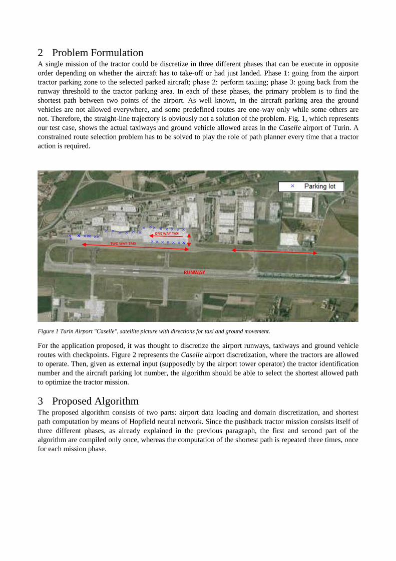
2 Problem Formulation A single mission of the tractor could be discretize in three different phases that can be execute in opposite

order depending on whether the aircraft has to take-off or had just landed. Phase 1: going from the airport

tractor parking zone to the selected parked aircraft; phase 2: perform taxiing; phase 3: going back from the

runway threshold to the tractor parking area. In each of these phases, the primary problem is to find the

shortest path between two points of the airport. As well known, in the aircraft parking area the ground

vehicles are not allowed everywhere, and some predefined routes are one-way only while some others are

not. Therefore, the straight-line trajectory is obviously not a solution of the problem. Fig. 1, which represents

our test case, shows the actual taxiways and ground vehicle allowed areas in the Caselle airport of Turin. A

constrained route selection problem has to be solved to play the role of path planner every time that a tractor

action is required.

Figure 1 Turin Airport "Caselle", satellite picture with directions for taxi and ground movement.

For the application proposed, it was thought to discretize the airport runways, taxiways and ground vehicle

routes with checkpoints. Figure 2 represents the Caselle airport discretization, where the tractors are allowed

to operate. Then, given as external input (supposedly by the airport tower operator) the tractor identification

number and the aircraft parking lot number, the algorithm should be able to select the shortest allowed path

to optimize the tractor mission.

3 Proposed Algorithm The proposed algorithm consists of two parts: airport data loading and domain discretization, and shortest

path computation by means of Hopfield neural network. Since the pushback tractor mission consists itself of

three different phases, as already explained in the previous paragraph, the first and second part of the

algorithm are compiled only once, whereas the computation of the shortest path is repeated three times, once

for each mission phase.

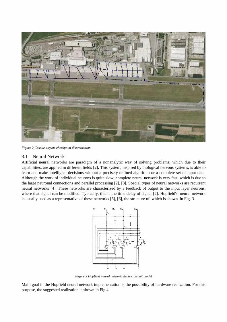
Figure 2 Caselle airport checkpoint discretization

3.1 Neural Network Artificial neural networks are paradigm of a nonanalytic way of solving problems, which due to their

capabilities, are applied in different fields [2]. This system, inspired by biological nervous systems, is able to

learn and make intelligent decisions without a precisely defined algorithm or a complete set of input data.

Although the work of individual neurons is quite slow, complete neural network is very fast, which is due to

the large neuronal connections and parallel processing [2], [3]. Special types of neural networks are recurrent

neural networks [4]. These networks are characterized by a feedback of output to the input layer neurons,

where that signal can be modified. Typically, this is the time delay of signal [2]. Hopfield's neural network

is usually used as a representative of these networks [5], [6], the structure of which is shown in Fig. 3.

Figure 3 Hopfield neural network electric circuit model

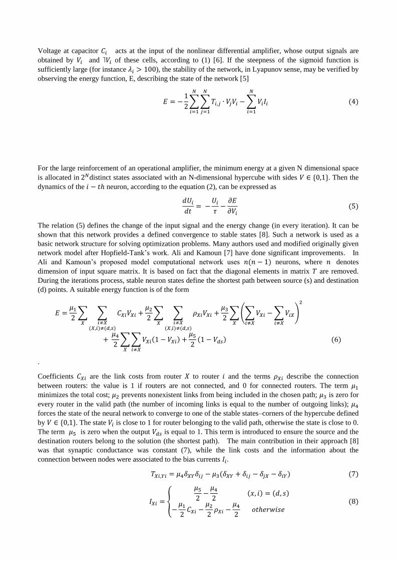
Main goal in the Hopfield neural network implementation is the possibility of hardware realization. For this

purpose, the suggested realization is shown in Fig.4.

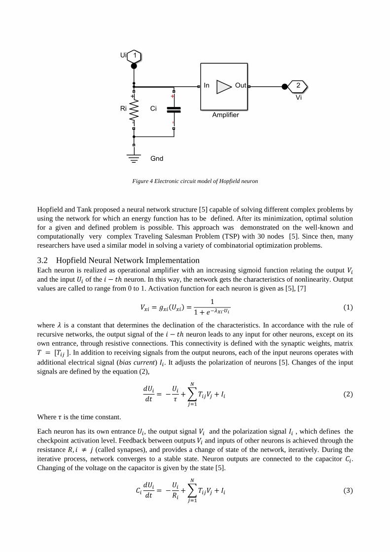
Figure 4 Electronic circuit model of Hopfield neuron

Hopfield and Tank proposed a neural network structure [5] capable of solving different complex problems by

using the network for which an energy function has to be defined. After its minimization, optimal solution

for a given and defined problem is possible. This approach was demonstrated on the well-known and

computationally very complex Traveling Salesman Problem (TSP) with 30 nodes [5]. Since then, many

researchers have used a similar model in solving a variety of combinatorial optimization problems.

3.2 Hopfield Neural Network Implementation Each neuron is realized as operational amplifier with an increasing sigmoid function relating the output 𝑉𝑖

and the input 𝑈𝑖 of the 𝑖 − 𝑡ℎ neuron. In this way, the network gets the characteristics of nonlinearity. Output

values are called to range from 0 to 1. Activation function for each neuron is given as [5], [7]

𝑉𝑥𝑖 = 𝑔𝑥𝑖(𝑈𝑥𝑖) =1

1 + 𝑒−𝜆𝑋𝑖∙𝑈𝑖 (1)

where 𝜆 is a constant that determines the declination of the characteristics. In accordance with the rule of

recursive networks, the output signal of the 𝑖 − 𝑡ℎ neuron leads to any input for other neurons, except on its

own entrance, through resistive connections. This connectivity is defined with the synaptic weights, matrix

𝑇 = [𝑇𝑖𝑗 ]. In addition to receiving signals from the output neurons, each of the input neurons operates with

additional electrical signal (bias current) 𝐼𝑖. It adjusts the polarization of neurons [5]. Changes of the input

signals are defined by the equation (2),

𝑑𝑈𝑖

𝑑𝑡= −

𝑈𝑖

𝜏+ ∑ 𝑇𝑖𝑗𝑉𝑗

𝑁

𝑗=1

+ 𝐼𝑖 (2)

Where 𝜏 is the time constant.

Each neuron has its own entrance 𝑈𝑖, the output signal 𝑉𝑖 and the polarization signal 𝐼𝑖 , which defines the

checkpoint activation level. Feedback between outputs 𝑉𝑖 and inputs of other neurons is achieved through the

resistance 𝑅, 𝑖 ≠ 𝑗 (called synapses), and provides a change of state of the network, iteratively. During the

iterative process, network converges to a stable state. Neuron outputs are connected to the capacitor 𝐶𝑖.

Changing of the voltage on the capacitor is given by the state [5].

𝐶𝑖

𝑑𝑈𝑖

𝑑𝑡= −

𝑈𝑖

𝑅𝑖+ ∑ 𝑇𝑖𝑗𝑉𝑗

𝑁

𝑗=1

+ 𝐼𝑖 (3)

Voltage at capacitor 𝐶𝑖 acts at the input of the nonlinear differential amplifier, whose output signals are

obtained by 𝑉𝑖 and ˥𝑉𝑖 of these cells, according to (1) [6]. If the steepness of the sigmoid function is

sufficiently large (for instance 𝜆𝑖 > 100), the stability of the network, in Lyapunov sense, may be verified by

observing the energy function, E, describing the state of the network [5]

𝐸 = −1

2∑ ∑ 𝑇𝑖,𝑗 ∙ 𝑉𝑗𝑉𝑖

𝑁

𝑗=1

𝑁

𝑖=1

− ∑ 𝑉𝑖𝐼𝑖

𝑁

𝑖=1

(4)

For the large reinforcement of an operational amplifier, the minimum energy at a given N dimensional space

is allocated in 2𝑁distinct states associated with an N-dimensional hypercube with sides 𝑉 ∈ {0,1}. Then the

dynamics of the 𝑖 − 𝑡ℎ neuron, according to the equation (2), can be expressed as

𝑑𝑈𝑖

𝑑𝑡= −

𝑈𝑖

𝜏−

𝜕𝐸

𝜕𝑉𝑖 (5)

The relation (5) defines the change of the input signal and the energy change (in every iteration). It can be

shown that this network provides a defined convergence to stable states [8]. Such a network is used as a

basic network structure for solving optimization problems. Many authors used and modified originally given

network model after Hopfield-Tank’s work. Ali and Kamoun [7] have done significant improvements. In

Ali and Kamoun’s proposed model computational network uses 𝑛(𝑛 − 1) neurons, where 𝑛 denotes

dimension of input square matrix. It is based on fact that the diagonal elements in matrix 𝑇 are removed.

During the iterations process, stable neuron states define the shortest path between source (s) and destination

(d) points. A suitable energy function is of the form

𝐸 =𝜇1

2∑ ∑ 𝐶𝑋𝑖𝑉𝑋𝑖

𝑖≠𝑋(𝑋,𝑖)≠(𝑑,𝑠)

𝑋

+𝜇2

2∑ ∑ 𝜌𝑋𝑖𝑉𝑋𝑖

𝑖≠𝑋(𝑋,𝑖)≠(𝑑,𝑠)

𝑋

+𝜇3

2∑ (∑ 𝑉𝑋𝑖

𝑖≠𝑋

− ∑ 𝑉𝑖𝑋

𝑖≠𝑋

)

𝑋

2

+ 𝜇4

2∑ ∑ 𝑉𝑋𝑖(1 − 𝑉𝑋𝑖)

𝑖≠𝑋𝑋

+𝜇5

2(1 − 𝑉𝑑𝑠) (6)

.

Coefficients 𝐶𝑋𝑖 are the link costs from router 𝑋 to router 𝑖 and the terms 𝜌𝑋𝑖 describe the connection

between routers: the value is 1 if routers are not connected, and 0 for connected routers. The term 𝜇1

minimizes the total cost; 𝜇2 prevents nonexistent links from being included in the chosen path; 𝜇3 is zero for

every router in the valid path (the number of incoming links is equal to the number of outgoing links); 𝜇4

forces the state of the neural network to converge to one of the stable states–corners of the hypercube defined

by 𝑉 ∈ {0,1}. The state 𝑉𝑖 is close to 1 for router belonging to the valid path, otherwise the state is close to 0.

The term 𝜇5 is zero when the output 𝑉𝑑𝑠 is equal to 1. This term is introduced to ensure the source and the

destination routers belong to the solution (the shortest path). The main contribution in their approach [8]

was that synaptic conductance was constant (7), while the link costs and the information about the

connection between nodes were associated to the bias currents 𝐼𝑖.

𝑇𝑋𝑖,𝑌𝑖 = 𝜇4𝛿𝑋𝑌𝛿𝑖𝑗 − 𝜇3(𝛿𝑋𝑌 + 𝛿𝑖𝑗 − 𝛿𝑗𝑋 − 𝛿𝑖𝑌) (7)

𝐼𝑋𝑖 = {

𝜇5

2−

𝜇4

2(𝑥, 𝑖) = (𝑑, 𝑠)

−𝜇1

2𝐶𝑋𝑖 −

𝜇2

2𝜌𝑋𝑖 −

𝜇4

2𝑜𝑡ℎ𝑒𝑟𝑤𝑖𝑠𝑒

(8)

Where 𝛿𝑖𝑖 = 1 , 𝛿𝑖𝑗 = 0, for 𝑖 ≠ 𝑗. In this way, the neural network algorithm becomes very attractive for real

time processing, since bias currents may be easily controlled via external circuitry following the changes in

actual traffic through the network. A number of papers show that HNN gives good results in problems

where finding the shortest or optimal path is necessary. Therefore, it was used in solving our problem. On the

other hand, the primary disadvantage of this network is its possible instability (for initialization of the

network with a noise signal) and the fact that the HNN does not always produce an optimal solution.

However, as Hopfield showed, if obtained solution is not optimal it will be in a group of solutions that are

very "close to" optimal.

4 Implementation and Results For the test purposes, complete code of the proposed algorithm is implemented in Matlab 8.1 without using

any pre-compiled toolbox. The code is optimized for the proposed test case, with the intention to make the

tool general and automatically adjustable to any airport selected from an available database. This tool is

supposed to be used by an airport control human operator, which should select the pushback tractor to use to

accomplish the mission, the aircraft (parked or just landed) to move, and the target destination.

4.1 Airport data loading and domain discretization To perform the route optimization problem the first step is the domain definition. This is done by

downloading the airport chart of interest from the official website containing the aeronautical information

publication (AIP), as reported in Appendix A for the proposed test case. It may contain the aircraft parking

docking locations in terms of latitude and longitude coordinates, otherwise docking locations, the taxiways

and allowed directions for tractors are only drawn. For this reason they can be discretized in checkpoints

manually from the chart by means of a getpoints function. The whole set of available checkpoint coordinates

are now indexed and stored in a matrix. The domain is then normalized to 1 with the maximum length of the

airport and the actual geographical distances between checkpoints are stored in a second matrix. An extra

matrix, called connectivity matrix, is built up containing all the connections and directions available between

nodes (Figure 5), as explained in section 3, the elements values are 0 between connected nodes 1 for not

connected nodes. The whole set of matrices represents the airport database named with its ICAO code.

4.2 Shortest path computation The second part of the algorithm starts loading the airport database on the workspace. Every

neuron/checkpoint of the net is initialized, the time evolution of the state of the neural network is simulated

by numerically solving (5). This corresponds to solving a system of 𝑛(𝑛 − 1) nonlinear differential

equations, where the variables are the neurons’ output voltages 𝑉𝑋𝑖’s. To achieve this, we have chosen the

fourth order Runge-Kutta method since it is sufficiently accurate and easy to implement. Accordingly the

simulation consisted of observing and updating the neuron output voltages at incremental time steps 𝛿𝑡,

chosen to be 10−5. In addition, the time constant 𝜏 of each neuron is set to 1 and for simplicity it is assumed

that 𝜆𝑋𝑖 = 𝜆 and 𝑔𝑋𝑖 = 𝑔 all independent of the subscript (𝑥, 𝑖). Another important parameter in the

simulation is the neuron initial input voltages 𝑈𝑥𝑖. Since the neural network should have no a prior favor for

a particular path, all the 𝑈𝑥𝑖’s should be set to zero. However some initial random noise −0.0002 ≤ 𝛿𝑈𝑥𝑖 ≤

+0.0002 helps to break the symmetry caused by symmetric network topologies and by the possibility of

having more than one shortest path. The simulation is stopped when the system reaches a stable final state.

This is assumed to occur when all neuron output voltages do not change by more than a threshold value of

Δ𝑉𝑡ℎ = 10−5 from one update to the next. At the stable state each neuron is either On (𝑉𝑋𝑖 ≥ 0.5) or Off

(𝑉𝑥𝑖 ≤ 0.5). The process is then repeated three time, once every pushback tractor mission phase. The

shortest path computed is finally displayed on the satellite map of the airport.

4.3 Test case results For testing purpose, an application to the Turin airport Caselle is implemented, Figure 2. A network of 56

checkpoints is created corresponding to the real airport parking lot and taxiways. The connectivity matrix,

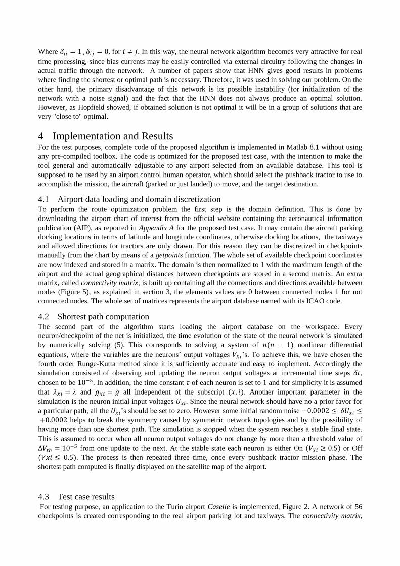
defined using Eq. (7), respects the airport regulations. Ones represent not connected nodes while the zeros

are existing connections. The matrix is not symmetric because some taxiways are one way only as previously

said.

Figure 5 Caselle airport, Network connectivity matrix

In the simulation, an appropriate sizing of the parameters is found by the general rules reported in [7].

Results in this section refer to parameter sets as:

𝜇1 = 922; 𝜇2 = 3500; 𝜇3 = 2500; 𝜇4 = 475; 𝜇5 = 3500.

The choice of network parameters that provides good solutions is a compromise between always obtain

legitimate tours (𝜇1 𝑠𝑚𝑎𝑙𝑙) and weighting the distances heavily (𝜇1 𝑙𝑎𝑟𝑔𝑒). Also, too small values of 𝜆 (low

gain) results in final states in which the values of 𝑉𝑋𝑖 are not near to 1 or 0. Too large values of λ yields a

poorer selection of good path. In this test case, it is set to 𝜆 = 50. Results of the simulations are reported for

Figure 6 to Figure 11, where two different pushback tractor missions are analyzed. The first is relative to an

aircraft departure in which the pushback tractor stars from the deposit area, then goes to pick up the airplane

to tow it to the takeoff position and finally goes back to the deposit area. The second mission is relative to a

tractor placed in a random position of the airport area, then goes to pick up the airplane at the landing

checkpoint to tow it in the appropriate parking lot and finally goes back to the deposit. Each figure shows

separately the three phases of which the mission is made of. The parameters are maintained constant during

the entire simulation test case. Algorithm convergence is obtained in a reasonable time and optimized paths

are depicted in figures with different colors.

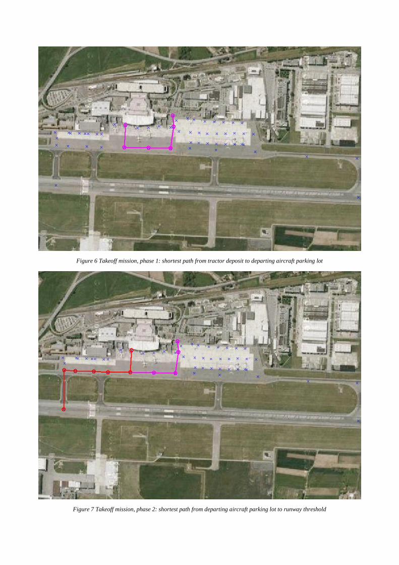
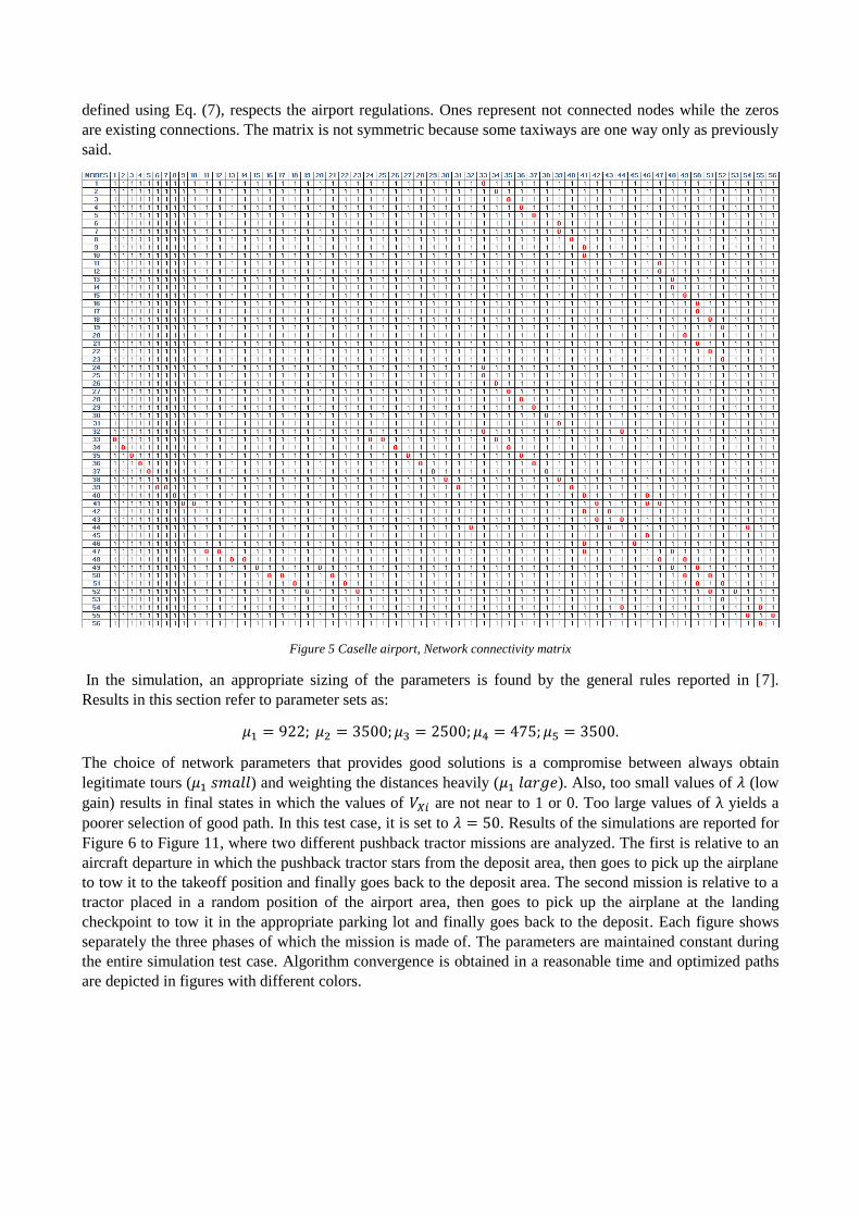
Figure 6 Takeoff mission, phase 1: shortest path from tractor deposit to departing aircraft parking lot

Figure 7 Takeoff mission, phase 2: shortest path from departing aircraft parking lot to runway threshold

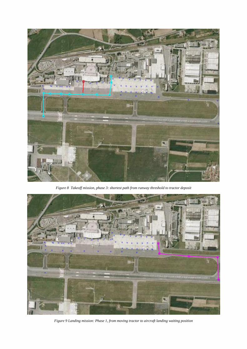
Figure 8 Takeoff mission, phase 3: shortest path from runway threshold to tractor deposit

Figure 9 Landing mission: Phase 1, from moving tractor to aircraft landing waiting position

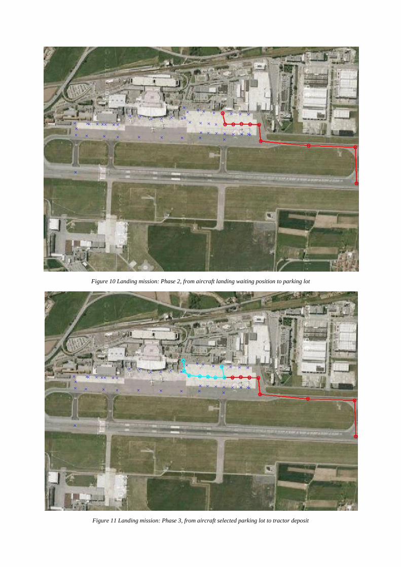
Figure 10 Landing mission: Phase 2, from aircraft landing waiting position to parking lot

Figure 11 Landing mission: Phase 3, from aircraft selected parking lot to tractor deposit

5 Conclusion This paper presents a software solution for the shortest path problem based on artificial intelligence and

applied to an innovative, fully automatic pushback tractor system. The proposed algorithm aims to discretize

any airport and its pathways, and computes in the most efficient way a feasible shortest route to accomplish

the mission. The mission is sequenced in three phases: going from the airport tractor-parking zone to the

selected parked aircraft; perform taxiing; and going back from the runway threshold to the tractor parking

area. For each phase, the same Hopfield neural network is used to successfully perform the computation.

Further work will be focused in the implementation and optimization of a graphical interface to help the user

in selecting the desired airport database, selecting the proper pushback tractor and aircraft to be towed from

screen. A communication interface will be also implemented to pass the obtained optimized path in terms of

checkpoints to the tractor autopilot still to be developed.

References

[1] M. Battipede, A. Della Corte, M. Vazzola and D. Tancredi, “Innovative Airplane Ground Handling

System for Green Operations”, 27th International Congress Of The Aeronautical Sciences, ICAS 2010.

[2] HAYKIN, S., Neural Networks–A Comprehensive Foundation. MacMillan collage Publishing

Company, Inc., 1994.

[3] RAHMAN, S. A., ANSARI, M. S., MOINUDDIN, A. A., Solution of linear programming problems

using a neural network with nonlinear feedback. Radioengineering, 2012, vol. 21, no. 4, p. 1171-1177.

[4] TOBES, Z., RAIDA, Z., Analysis of recurrent analog neural networks. Radioengineering, 1998, vol.

7, no. 2, p. 9-14.

[5] HOPFIELD, J. J., TANK, D. W. Neural’ computations of decision in optimization problems. Biol.

Cybern., 1985, p. 141–152.

[6] HOPFIELD, J. J., Neural networks and physical systems with emergent collective computational

abilities. Proc. Nat. Acad. Sci., 1982, vol. 79, p. 2554–2558.

[7] ALI, M., KAMOUN, F., Neural networks for shortest path computation and routing in computer

networks. IEEE Trans. On Neural Networks, 1993, vol. 4, no. 6, p. 941–953.

[8] WASSERMAN, P. D. Advanced Methods in Neural Computing. New York: Van Nostrand

Reinhold, 1993.

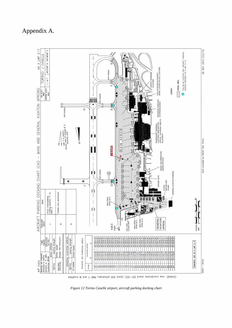
Appendix A.

Figure 12 Torino Caselle airport, aircraft parking docking chart