A robust triangular membrane element - SciELO · r 2 vu r xy ¶¶ =-¶¶ (3) In the common finite...

2648

Abstract To analyze the plane problem with irregular mesh and complicat-ed geometry, it is helpful to utilize the triangular element. In this study, several optimization criteria will be elaborated. By utilizing these provisions and satisfying the equilibrium conditions, a novel triangular element, named SST, is developed. To demonstrate the high accuracy and efficiency of the new element, a variety of structures will be solved. The findings will prove that the present-ed element has a low sensitivity to the geometric distortion. More-over, the parasitic shear error will not arise when this element is employed. In addition to these, the proposed element is rotational invariant. Comparison studies will reveal that the SST element is more robust than the other well-known triangular ones. Keywords Finite element; optimal criteria; geometric distortion; triangular element; plane problem; parasitic shear.

A robust triangular membrane element

1 INTRODUCTION

Different types of formulation have been created since 1980s. The two most famous ones are named free formulation (Bergan and Nygard, 1984) and assumed strain technique (MacNeal, 1978). Based on these strategies, the high-performance elements were formulated. Some of the noticeable charac-teristics of these elements are: simplicity, rotational invariance, rank sufficiency, rapid convergence, yielding similar accuracy in displacements and strains, insensitivity to geometric distortion. They are also mixable with the other elements (Felippa, 1994). During the period of 1990-2000, the parameterized variational principle severely changed the knowledge towards highly efficient element formulations. By utilizing this principle, researchers managed to define a continuous space of the elastic functional. In the early 1990s, the parameter-ized variational principle was applied successfully in the finite element scheme. Consequently, the formulation of high-performance elements was developed more fully, based on a continuous space of the elastic functionals. Making stationary of the continuous space of the functional, produces free parameters for the formulation of the element (Felippa and Militello, 1990). As a result, this will lead to finite element templates. It should be added, the process of optimizing finite element tem-

M. Rezaiee–Pajand*

M. Yaghoobi. Civil Engineering Department, Fer-dowsi University of Mashhad, Iran

*Corresponding author: [email protected] Received 28.12.2013 In revised form 22.05.2014 Accepted 23.07.2014 Available online 17.08.2014

2649 M. Rezaiee-Pajand and M. Yaghoobi / An efficient formulation for linear and geometric non-linear membrane elements

Latin American Journal of Solids and Structures 11 (2014) 2648-2671

plates is quite complex, and requires innovations. The large number of the free parameters, symbol-ic processing and optimizing the entries of the matrix are among the difficulties, which are encoun-tered in the mentioned process. Two investigators, named Bergan and Nygard, developed the free formulation (Bergan and Ny-gard, 1984). In the related area, John Dow et al. proposed another scheme named strain gradient notation (Dow, 1999). Within this procedure, the displacement interpolation field is expressed in terms of strain states. In this way, the roots of many errors in the finite-element scheme can be explored and eliminated. It should be mentioned that strain gradient notation is an explicit and simple representation of the free formulation approach. It is possible to utilize this approach and write displacements and also strains in terms of strain states. Furthermore, some optimal criteria will generally be included to enhance the outcomes of the element. By using these optimality crite-ria the resultant element is rotational invariance and insensitive to geometry distortion. Moreover, the parasitic shear error is eliminated, and the equilibrium equations are satisfied in this formula-tion. In this paper, strain states formulation is presented, and a new triangular element, named SST, is suggested. It is worth emphasizing that the recommended element is useful to analyze the plane problems with irregular mesh and complicated geometry. In fact, the triangular elements are able to model the geometry of the structure more properly. On the other hand, numerical experiences have shown that the low-order triangular elements are less accurate than the quadrilateral ones (Eom et al., 2009). To solve irregular meshes, various means of constructing triangular elements have been proposed by the researchers (Felippa, 2003a; Choo et al., 2006; Huang et al., 2010; Pan and Wheel, 2011; Caylak and Mahnken, 2011;). In the following sections; several numerical tests are performed to demonstrate the capabilities of the suggested element. The obtained results indicate good ele-mental performances, such as high accuracy, low sensitivity to geometry distortion, rotational invar-iance and rapid convergence. 2 STRAIN GRADIENT NOTATION FORMULATION

In strain gradient notation, Taylor's expansion of the strain field is utilized about the coordinates’ origin (Dow, 1999). In the two-dimensional state, the strain field consists of three strain function as follows:

2 2

, , , , ,

2 2

, , , , ,

2

, , ,

( , ) ( ) ( ) ( ) ( ) ( ) ( ) ( ) ( ) ( ) ...2 2

( , ) ( ) ( ) ( ) ( ) ( ) ( ) ( ) ( ) ( ) ...2 2

( , ) ( ) ( ) ( ) ( ) (

x x o x x o x y o x xx o x xy o x yy o

y y o y x o y y o y xx o y xy o y yy o

xy xy o xy x o xy y o xy xx o

x yx y x y xy

x yx y x y xy

xx y x y

e e e e e e e

e e e e e e e

g g g g g

= + + + + + +

= + + + + + +

= + + +2

, ,) ( ) ( ) ( ) ( ) ...2 2

.xy xy o xy yy oy

xyg g+ + +

(1)

In these equations, as a subscript denotes the strain gradient value at the origin. These values are called strain states. The magnitude of axial strain xe at the origin is denoted by ( )x oe , ,( )x x oe and ,( )x y oe are the rate of xe variation in x and y directions, in the origin’s vicinity, respectively. Similarly, other coefficients can be determined. The displacement field is calculated by using strain-displacement equations and rotation function, which are given in below:

M. Rezaiee-Pajand and M. Yaghoobi / An efficient formulation for linear and geometric non-linear membrane elements 2650


xu

xe

¶=

¶, y

v

ye

¶=

¶, xy

u v

y xg

¶ ¶= +

¶ ¶ (2)

1( )

2rv u

rx y

¶ ¶= -

¶ ¶ (3)

In the common finite element formulation, the displacements are interpolated using a polynomial field function similar to the below form:

2 21 2 3 4 5 6

2 21 2 3 4 5 6

( , ) ...

( , ) ...

u x y a a x a y a x a xy a y

v x y b b x b y b x b xy b y

ìï = + + + + + +ïïíï = + + + + + +ïïî (4)

At the origin, strains and rotation will have the following values:

2 3

2

3

2 3

( ) ( ) / 2

( )

( )

( )

r

x

y

xy

r b a

a

b

b a

eeg

ì = -ïïïï =ïïíï =ïïï = +ïïî

(5)

The rigid body rotation is equal to ( )rr . The unknown parameters are written in terms of strains as below:

2

3

2

3

( )

( / 2 )

( / 2 )

( )

x

xy r

xy r

y

a

a r

b r

b

egge

ì =ïïïï = -ïïíï = +ïïï =ïïî

(6)

The coefficients of the quadratic terms of the field interpolation function can be determined by a similar approach. For this purpose, the next derivatives of the strains are utilized:

2 2

, ,2

2 2

, , 2

2 2 2 2

, ,2 2

,

,

,

x xx x x y

y yy x y y

xy xyxy x xy y

u u

x y x yxv v

x y x y y

u v u v

x y x y x yx y

e ee e

e ee e

g gg g

¶ ¶¶ ¶= = = =

¶ ¶ ¶ ¶¶¶ ¶¶ ¶

= = = =¶ ¶ ¶ ¶ ¶¶ ¶¶ ¶ ¶ ¶

= = + = = +¶ ¶ ¶ ¶ ¶ ¶¶ ¶

(7)

By replacing the coordinates of the origin and solving the resulting set of equations; the coeffi-cients of the displacement interpolation functions are determined, as follows:

4 , 4 , ,

5 , 5 ,

6 , , 6 ,

( ) / 2, ( ) / 2

( ) , ( )

( ) / 2, ( ) / 2

x x xy x x y

x y y x

xy y y x y y

a b

a b

a b

e g ee eg e e

= = -= == - =

(8)



The remaining coefficients of the displacement interpolation field are obtained in a similar man-ner. Let u and v be the rigid body translations along the x and y axes, based on this assump-tion; the element's field functions will have the below form:

2 2, , , ,

2 2, , , ,

( ) ( / 2 ) ( ) / 2 ( ) ( ) / 2 ...

( / 2 ) ( ) ( ) / 2 ( ) ( ) / 2 ...x xy r x x x y xy y y x

xy r y xy x x y y x y y

u u x r y x xy y

v v r x y x xy y

e g e e g e

g e g e e e

ìï = + + - + + + - +ïïíï = + + + + - + + +ïïî

(9)

3 OPTIMALITY CONDITIONS

In order to attain the efficient elements, the optimization condition can be inserted into the formu-lation. In this approach, the roots of many errors may be recognized. Several optimality constraints are included in the authors' formulation, which are discussed in the coming sections. 3.1 Satisfying the equilibrium equations

To solve the plane problems in the plane-stress or plane-strain state, the equilibrium relations have to be satisfied. For a homogeneous elastic continuum, these equations are written in the following shape:

( , )( , )( , ) 0

( , ) ( , )( , ) 0

xyxx

xy yy

x yx yF x y

x yx y x y

F x yx y

ge

g e

ì ¶ï¶ïï + + =ï ¶ ¶ïïíï¶ ¶ïï + + =ïï ¶ ¶ïî

(10)

In these equalities, the functions ( , )xF x y and ( , )yF x y are the force field functions along the x and y directions in a rectangular coordinate system, respectively. It is obvious that in the planar problems, gradient of the force field, in the perpendicular direction (z) to plane of the element, is equal to zero. To include the stress fields, they are defined in the rectangular coordinate system. Utilizing the stress-strain relations, Eq. (10) can be rewritten in terms of the strain fields. Based on the Hooke's law for a homogeneous elastic condition, the following relations are valid for a plane problem:

2 ( )

2 ( )x x x y

y y x y

xy xy

G

G

G

s e l e es e l e et g

= + +

= + +=

(11)

In these formulas, l for the plane-strain and plane-stress cases will be equal to

(1 )(1 2 )

Enn n+ -

, and (1 )(1 )

Enn n+ -

,

respectively. The shear modulus, Poisson's ratio, and elastic modulus are denoted by G, n and E, correspondingly. The next equilibrium equations will be established by inserting Eq. (11) into Eq. (10):



( , ) ( , )( , )(2 ) ( , ) 0

( , ) ( , )( , )(2 ) ( , ) 0

y xyxx

y xyxy

x y x yx yG G F x y

x x yx y x yx y

G G F x yy y x

e gel l

e gel l

ì ¶ ¶ï ¶ïï + + + + =ï ¶ ¶ ¶ïïíï ¶ ¶¶ïï + + + + =ïï ¶ ¶ ¶ïî

(12)

3.2 Planar pure bending test

This examination has been utilized for finding the optimal flexural template by Felippa (Felippa, 2003a, 2003b, 2006). In this work, Euler-Bernoulli beam has been applied to assess response of the template to the in-plane bending along the x and y axes. The energy ratios (r) are measured in this experiment. Two parameters, named xr and yr , denote the bending energy ratios of the beam’s rectangular part in x and y directions, respectively. Fig. (1) shows a simple structure to be utilized in studying the bending behavior of a beam in the x direction. This structure has a cross section equal to b h´ , with a moment of xM at the free ends.

Figure 1: In-plane pure bending test along the x axes.

Ignoring the complicated behavior of the two ends, the majority of the beam will undergo a con-stant bending moment of ( ) xM x M= , which will produce a stress field equal to /x x bM y Is = - . Noting that 3 / 12bI hb= and 0y xys t= = . To study the structural behavior in the y direction, the beam of Fig. (2) is assumed. This structure is subject to yM at the free ends. The bending mo-ment along the beam is equal to ( ) yM y M= , which results in a the stress field of /y y aM x Is = - , with 3 / 12aI ha= and 0x xys t= = . It should be added that these are exact results obtained from the elastic theory of the beams. Based on the aforementioned discussions, the internal elastic energy, which is stored in the a b´ section of this beam, has the following value:

2

3

2

3

6

6

beam xx

ybeamy

aMU

Eb hbM

UEa h

=

=

(13)

In addition, the potential energy of the a b´ section is also calculated when the beam is subject-ed to xM and yM . It is clear from Figs. (1) and (2), the moments xM and yM will bend the struc-



ture in the xy plane. If this section is composed of only one rectangular element, the potential ener-gy can be written in the coming form:

Figure 2: In-plane pure bending test along the y axes.

1

21

2

panel Tx bx bx

panel Ty by by

U

U

=

=

D KD

D KD (14)

Where, bxD and byD are the nodal displacement vectors corresponding to relevant stress fields re-sulted from xM and yM moments, respectively. The stiffness matrix of the rectangular element is denoted by K . It should be mentioned that this test can also be used for triangular elements. In this case, the potential energy is equal to the sum of the potential energies stored in the two trian-gular elements, which is composed of section a b´ . The displacements bxD and byD are essential to evaluate this potential energy. For this purpose, stress fields are obtained for both cases of in-plane bending, which are shown in Figs. (1) and (2). These stress functions have the following relations:

3

3

12, 0, 0

120, , 0

xx y xy

yx y xy

M y

b hM x

a h

s s t

s s t

= - = =

= = = (15)

With stresses functions at hand, the strain field can be attained. Afterwards, the displacement fields are obtained by integration. The flexural energy ratios for the x and y directions are calculated in the coming shapes:



panelx

x beamxpanely

y beamy

Ur

U

Ur

U

=

=

(16)

Based on these parameters, an element will be capable of correctly represent the bending in any arbitrary directions, when 1xr = and 1yr = ( 1r = ). It should be added that an element will be over stiff or over flexible while 1r or 1r . In the case of 1r = , any aspect ratio of the element will have optimum behavior in bending. Furthermore, if (r) increases as the aspect ratio rises, the locking shear will appear in the element. At this stage, this test will be investigated based on the strain states. In planar bending in x direction, the real stress field varies linearly along the y direction. According to the Hook’s law, this strain state has the coming shape:

1 2 3 4 , , 0x y xyy ye b b e b b g= + = + = (17) In the last relationships, 1b , 2b , 3b and 4b are all constant coefficients. Equations (17) indi-cates that only ( )x oe , ( )y oe , ,( )x y oe and ,( )y y oe participate in the aforementioned strain field. Similar-ly, if the beam is subjected to yM , ( )x oe , ( )y oe , ,( )x x oe and ,( )y x oe are incorporated into the real strain field. Hence, ( )x oe , ( )y oe , ,( )x x oe , ,( )x y oe , ,( )y x oe and ,( )y y oe are required for achieving the actual solution for an in-plane flexural problem. A necessary condition for convergence requires that the element assumed strain field should always include constant strain states and the rigid motions' ones. It is worth emphasizing that the planar bending test based on the strain states does not im-pose any limitations on the geometric shape of the element. In other words, not only it can be uti-lized for triangular and rectangular elements, but other elements as well. 3.3 Rotational invariance

In the suitable elements, properties of the element will not alter with rotation of the coordinate system. These types of elements fall into the category of rotational invariance ones. It is obvious that elements can be configured with different rotational orientation in the mesh of a structure. Therefore, the element should be rotational invariance. To have this important property, terms of the strain field with a complete order should be selected (Dow, 1999; Rezaiee-Pajand and Yaghoobi, 2012, 2013, 2014). For instance, the rotational mapping of a constant strain state has the next ap-pearances:

2 2

2 2

2 2

( ) ( ) cos ( ) sin ( ) sin cos

( ) ( ) sin ( ) cos ( ) sin cos

( ) 2(( ) ( ) )sin cos ( ) (cos sin )

x x y xy

y x y xy

x y y x xy

e e q e q g q q

e e q e q g q q

g e e q q g q q

¢

¢

¢ ¢

= + +

= + -

= - + -

(18)

According to these relationships, only if the formulation takes into account all three cases of the constant strain states, then an element is capable of representing constant strains with respect to



any system of the coordinates. It should be stated that invariance constraint has been used by other researchers in the process of developing fine element templates (Felippa and Militello, 1999; Felippa, 2000).

3.4 Lack of the parasitic shear error

The existence of axial strain states in the shear strain interpolation function causes the parasitic shear effect. This bad property will lead to stiffen of the element (Dow, 1999). To grow the knowledge about parasitic shear error, formulation of the four-node rectangular element is examined in the coming lines. This element employs an incomplete polynomial, which contains neither 2x nor

2y terms. The strain gradient notation related to these terms can be represented in the following form:

,

,

( ) ( / 2 ) ( )

( / 2 ) ( ) ( )x xy r x y

xy r y y x

u u x r y xy

v v r x y xy

e g eg e e

ì = + + - +ïïíï = + + + +ïî

(19)

Based on the strain-deformation relations, which were given by Equations (2), the interpolation functions of the element can be written in the coming shapes:

,

,

, ,

( , ) ( ) ( )

( , ) ( ) ( )

( , ) ( ) ( ) ( )

x x x y

y y y x

xy xy x y y x

x y y

x y x

x y x y

e e ee e eg g e e

= +

= +

= + +

(20)

To find the advantages and deficiencies of this model, the Taylor's expansion of the polynomial should be considered. From the shear strain series, it is observed that the shear strains are inde-pendent of the axial strain. Two strain states, ,( )x y oe and ,( )y x oe , improperly appear in the shear strain interpolation function. As a result, if the element undergoes flexural deformations, the strain states will be nonzero and will incorrectly represent a portion of the shear strain. It is very important to know, if any element is formulated by using the strain gradient notation, the parasitic shear error can be easily eliminated by excluding the incorrect strain states from the shear strain polynomial. In fact, the parasitic shear error decreases as the finer meshes are utilized. As a result, even coarser meshes can produce good responses if elements are exempted from this error. Furthermore, utilizing the complete interpolation functions will prevent the appearance of this error. Including these important issues in the new formulation, the following strain states will be used for the model:

, , , , , ,, ,( ) ,( ) ,( ) ,( ) ,( ) ,( ) ,( ) ,( ) ,( ) ,( )r x y xy x x x y y x y y xy x xy yu v r e e g e e e e g g (21)

4 LINEAR FORMULATION

Based on the strain states in Eq.(21), the displacement field of this model is defined as below:



2 2, , , ,

2 2, , , ,

( ) ( / 2 ) ( ) / 2 ( ) ( ) / 2

( / 2 ) ( ) ( ) / 2 ( ) ( ) / 2x xy r x x x y xy y y x

xy r y xy x x y y x y y

u u x r y x xy y

v v r x y x xy y

e g e e g e

g e g e e e

ìï = + + - + + + -ïïíï = + + + + - + +ïïî

(22)

The coming strain field is also utilized:

, ,

, ,

, ,

( , ) ( ) ( ) ( )

( , ) ( ) ( ) ( )

( , ) ( ) ( ) ( )

x x x x x y

y y y x y y

xy xy xy x xy y

x y x y

x y x y

x y x y

e e e ee e e eg g g g

= + += + += + +

(23)

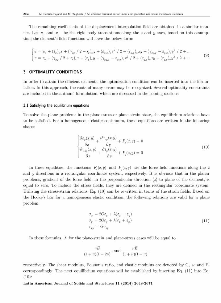
It should be added that x-y coordinate is a generalized one, and can be set up in any optional places. Based on formula (23), Eq. (12) can be written as below:

, ,,

, ,,

(2 )( ) ( )( )

( ) (2 )( )( )

x x y xxy y

x y y yxy x

G

GG

G

l e l eg

l e l eg

ì + +ïïï = -ïïíï + +ïï = -ïïî

(24)

According to these relationships, the body forces are assumed to be zero. In the formulas (24), both strain states, ,( )xy x og and ,( )xy y og can be expressed as a function of other strain states. By using these equations, the number of the unknowns will be decreased to 10. Furthermore, the vector of the strain states has the next shape:

, , , ,[ ( ) ( ) ( ) ( ) ( ) ( ) ( ) ( ) ]Tr x y xy x x y x x y y yu v r e e g e e e e=q (25)

Using this notion, the strain interpolation field can be represented in the below matrix form:

qe = B .q (26)

0 0 0 1 0 0 0 0

0 0 0 0 1 0 0 0

(2 ) (2 )0 0 0 0 0 1

q

x y

x y

G Gy y x x

G G G G

l ll l

é ùê úê úê ú

= ê úê úê ú+ +

- - - -ê úê úë û

B (27)

In addition, the displacement interpolation field has the following matrix shape:

qu = N .q (28) 2 22

2 22

(2 ) ( )1 0 0 0

2 2 2 2( ) (2 )

0 1 0 02 2 2 2

q

G y G yy xy x xy

G GG x G xx y

x y xyG G

l l

l l

é ù+ +ê ú- - -ê ú= ê ú

ê ú+ +ê ú- -ê úë û

N (29)

Introducing nodal coordinates into relation (28) yields the coming result:



qD = G .q (30) In the last relationship, D denotes the displacement vector. The qG matrix is obtained by in-serting the nodal coordinates into qN . It is obvious that qG provides a relation between the strain state vector and the displacement one. The boundary conditions should be applied to the formula-tion. To have displacements and strains' interpolation fields in terms of nodal values, these func-tions can be expressed in the succeeding form:

1q q q

-u = N .q = N .G .D = N.D (31)1

q q qe -= B .q = B .G .D = B.D (32) The potential energy function, which is in terms of the elastic matrix (E ), should be minimized in the coming shape:

1

2T Tdv dve eP = - =ò ò.E. U .F 0 (33)

¶P=

¶0

D (34)

( )T Tdv dv- =ò òB .E.B .D N .F 0 (35)

The last formula leads to the structural stiffness matrix. This matrix, which is denoted by K , has the below form:

T dv= òK B .E.B (36)

5 CREATION OF A SPECIAL ELEMENT

The effectiveness of the formulation is verified through the creation of a special element. For this purpose, the aforementioned model will be applied to a triangular element. As it was previously mentioned, ten nodal unknowns should be identified to formulate the element. The geometry of the proposed element is shown in Fig. (3).

Figure 3: The element degrees of freedom.



It is obvious that any adjacent two elements forms generalized four-sided elements. This is shown in Fig. (3-2). First, a mesh with quadrilateral elements is defined. By using diameter line, each four-sided element is divided into two triangular elements, as it is shown in Figure (3.2). All of these diameter lines have six degrees of freedom. In each element, the nodes located on the middle of diameter lines contain ninth and tenth degrees of freedom. To calculate qG , the displacement in the direction perpendicular to the side of the element is expressed in terms of u and v. This process is carried out for the side of ij in Fig. (4).

Figure 4: The degree of freedom perpendicular to the ij side.

( ) ( )sin ( )cosn m m mu u va a= - (37)

6 NUMERICAL STUDIES

In order to gain insight into the effectiveness of the proposed triangular element, several benchmark problems, which are introduced by other researchers, will be solved. These structures have formerly been used by the other investigators for testing a variety of different elements, and their results are available. The efficiency of the SST element in comparison to the other researchers’ well-known elements is evaluated via these plane problems. The mentioned elements are listed below: Triangular elements: ALL-3i : Allman 88 element integrated by 3-point interior rule (Allman, 1988; Felippa, 2003a). ALL-3m : Allman 88 element integrated by 3-midpoint rule (Allman, 1988; Felippa, 2003a). ALL-EX : Allman 88 element, exactly integrated (Allman, 1988; Felippa, 2003a). ALL-LS : Allman 88 element, least-square strain fit (Allman, 1988; Felippa, 2003a). Allman: Allman's element with spurious mode control (Allman, 1984; Cook, 1986; Choo et al., 2006; Eom et al., 2009). CST : Constant strain triangle CST-3/6C (Turner et al., 1956; Felippa, 2003a). CSTHybrid: Cook's plane hybrid triangle (Felippa, 2003a; Eom et al., 2009). FF84 : Free Formulation element of Bergan and Felippa (Bergan and Felippa, 1985; Felippa, 2003a). HT: The hybrid Trefftz (HT) plane element (Jirousek and Venkatesh, 1992; Choo et al., 2006). HTD: hybrid Trefftz plane elements with drilling degrees of freedom (Choo et al., 2006). LST-Ret : Retrofitted LST with ( 4 / 3ba = ) (Felippa, 2003a).

MEAS: The modified enhanced assumed strain triangle (Yeo and Lee, 1996, 1997; Choo et al., 2006;



Eom et al., 2009). OPT : Optimally fabricated assumed natural deviatoric strain triangle (Felippa, 2003a; Eom et al., 2009). OPT*: Optimally fabricated assumed natural deviatoric strain triangle with alternative formulation for higher-order stiffness matrix (Paknahad et al., 2007). SM3: The macro element with tuned higher-order stiffness parameter (Eom et al., 2009). Quadrilateral elements: AGQ6-II: Element with internal parameters and formulated by the QACM-I (Chen et al., 2004; Cen et al., 2009). EADG4: Enhanced assumed displacement gradient element with four modes (Wisniewski and Turska, 2008, 2009). HR5-S: HR element with five modes in skew coordinates (Wisniewski and Turska, 2006, 2009). HW12-S, HW14-S, HW10-N, HW14-N, HW18: Mixed four-node elements based on the Hu–Washizu functional (Wisniewski and Turska, 2009). PS: Stress hybrid element (Pian and Sumihara, 1984; Chen et al., 2004; Cen et al., 2009). Q4: Four-node isoparametric element (Chen et al., 2004; Wisniewski and Turska, 2009). Q6: Non-conforming isoparametric element with internal parameters (Wilson et al., 1973; Cen et al., 2007, 2009). QM6: Non-conforming isoparametric element with internal parameters (Taylor et al., 1976; Chen et al., 2004; Choi et al., 2006; Cen et al., 2009). 6.1 Short cantilever beam under shear force

The first example is a short homogeneous cantilever beam, which is subjected to a parabolic shear force at its free end. In order to model the fixity at the other end of the beam, the nodal displace-ments on that side are set to zero. The exact deflection of the free end is equal to 0.35601 (Felippa, 2003a). As illustrated in Fig. (5), the beam has a length of 48, height of 12 and width of 1. The elastic modulus is equal to 30000, and the Poisson's ratio is 0.25. All the related values of this ex-ample are dimensionless. The total shear load acting on the beam is equal to 40.

Figure 5: Short cantilever beam under shear force.



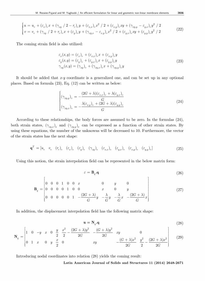
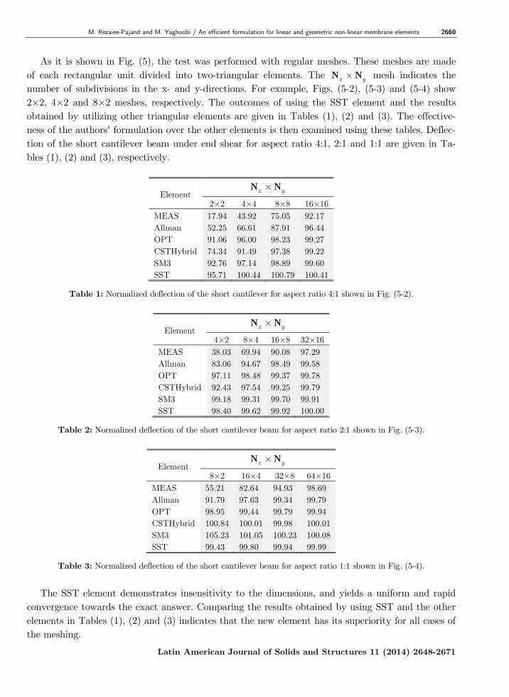
As it is shown in Fig. (5), the test was performed with regular meshes. These meshes are made of each rectangular unit divided into two-triangular elements. The x yŃ N mesh indicates the number of subdivisions in the x- and y-directions. For example, Figs. (5-2), (5-3) and (5-4) show 2×2, 4×2 and 8×2 meshes, respectively. The outcomes of using the SST element and the results obtained by utilizing other triangular elements are given in Tables (1), (2) and (3). The effective-ness of the authors' formulation over the other elements is then examined using these tables. Deflec-tion of the short cantilever beam under end shear for aspect ratio 4:1, 2:1 and 1:1 are given in Ta-bles (1), (2) and (3), respectively.

Element x yŃ N

2×2 4×4 8×8 16×16MEAS 17.94 43.92 75.05 92.17 Allman 52.25 66.61 87.91 96.44 OPT 91.06 96.00 98.23 99.27 CSTHybrid 74.34 91.49 97.38 99.22 SM3 92.76 97.14 98.89 99.60 SST 95.71 100.44 100.79 100.41

Table 1: Normalized deflection of the short cantilever for aspect ratio 4:1 shown in Fig. (5-2).

Element x yŃ N

4×2 8×4 16×8 32×16MEAS 38.03 69.94 90.08 97.29 Allman 83.06 94.67 98.49 99.58 OPT 97.11 98.48 99.37 99.78 CSTHybrid 92.43 97.54 99.25 99.79 SM3 99.18 99.31 99.70 99.91 SST 98.40 99.62 99.92 100.00

Table 2: Normalized deflection of the short cantilever beam for aspect ratio 2:1 shown in Fig. (5-3).

Element x yŃ N

8×2 16×4 32×8 64×16MEAS 55.21 82.64 94.93 98.69 Allman 91.79 97.63 99.34 99.79 OPT 98.95 99.44 99.79 99.94 CSTHybrid 100.84 100.01 99.98 100.01SM3 105.23 101.05 100.23 100.08SST 99.43 99.80 99.94 99.99

Table 3: Normalized deflection of the short cantilever beam for aspect ratio 1:1 shown in Fig. (5-4).

The SST element demonstrates insensitivity to the dimensions, and yields a uniform and rapid convergence towards the exact answer. Comparing the results obtained by using SST and the other elements in Tables (1), (2) and (3) indicates that the new element has its superiority for all cases of the meshing.



6.2 Slender cantilever beam under moment

The second benchmark problem is a homogeneous slender cantilever beam. This structure will be subjected to a bending moment at the free end. The nodes at the fixed end will have zero displace-ments. Based on the beam theory, the deflection of the free end of a beam with length L, moment of inertia zI and elastic modulus E , under a bending moment M will be equal to 2 / (2 )zML EI . In this equation, 3 / 12zI hb= . The elastic modulus E and the Poisson's ratio ν are set to 768 and 0.25, respectively. As it is illustrated in Fig. (6), the length of the beam is 32, the height is 2, and the width is equal to 1h = . The bending moment applied to this beam is equal to 100M = . The exact deflection of the beam's free end is equal to 100 (Felippa, 2003a).

Figure 6: Slender cantilever beam.

Regular meshes ranging from 2×2 to 32×2 are used, each rectangle mesh unit consisting of four half-thickness overlaid triangles. The element aspect ratios vary from 1:1 to 16:1. The deflection of the homogeneous slender cantilever beam under a moment at its free end is given in Table (4). Ta-ble (4) indicates that SST and OPT elements are more efficient than the other ones. The error of SST is less than one percent for all cases of the meshing.

Element x y´N N

2×2 4×2 8×2 16×2 32×2ALL-3I 0.39 5.42 38.32 76.48 87.08ALL-3M 0.04 0.71 9.59 53.57 81.36ALL-EX 0.16 2.47 24.23 69.09 84.90ALL-LS 0.12 1.89 20.83 68.25 85.36CST 1.28 4.82 15.75 36.36 54.05FF84 96.27 96.34 96.58 97.17 98.36LST-Ret 9.46 28.93 59.58 81.04 89.05OPT 100.07 99.96 99.99 99.99 99.99SST 99.09 99.49 99.75 99.88 99.92

Table 4: Free-end deflection of the slender beam under moment.

6.3 Thin cantilever beam

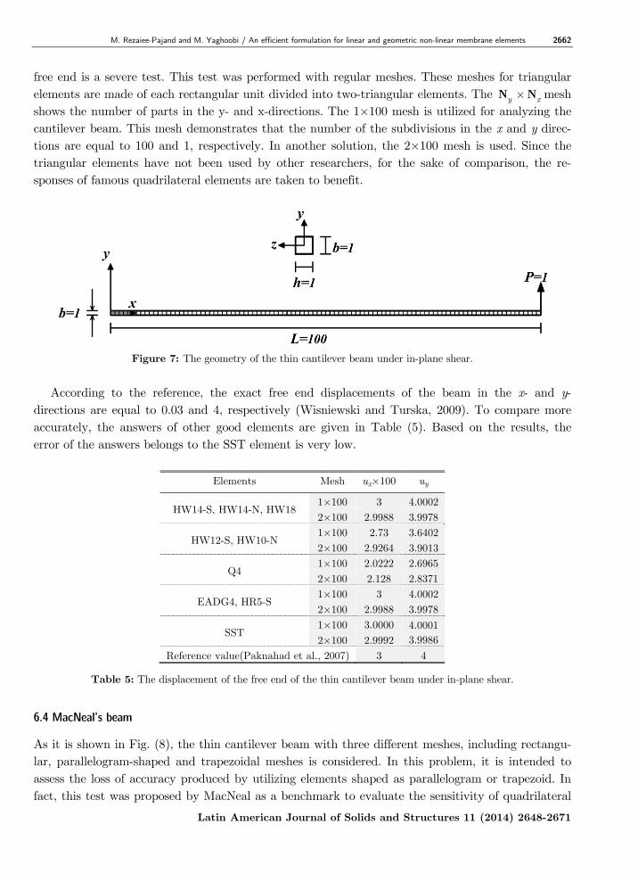
As it is shown in Fig. (7), the cantilever beam, which is under in-plane shear, has the length of 100, width of 1 and thickness of 1. The elasticity modulus and the Poisson ratio of this structure are equal to 1000000 and 0.3, respectively. It is important to note that this beam with a force of 1 at its



free end is a severe test. This test was performed with regular meshes. These meshes for triangular elements are made of each rectangular unit divided into two-triangular elements. The y x´N N mesh shows the number of parts in the y- and x-directions. The 1×100 mesh is utilized for analyzing the cantilever beam. This mesh demonstrates that the number of the subdivisions in the x and y direc-tions are equal to 100 and 1, respectively. In another solution, the 2×100 mesh is used. Since the triangular elements have not been used by other researchers, for the sake of comparison, the re-sponses of famous quadrilateral elements are taken to benefit.

Figure 7: The geometry of the thin cantilever beam under in-plane shear.

According to the reference, the exact free end displacements of the beam in the x- and y-directions are equal to 0.03 and 4, respectively (Wisniewski and Turska, 2009). To compare more accurately, the answers of other good elements are given in Table (5). Based on the results, the error of the answers belongs to the SST element is very low.

Elements Mesh ux×100 uy

HW14-S, HW14-N, HW18 1×100 3 4.00022×100 2.9988 3.9978

HW12-S, HW10-N 1×100 2.73 3.64022×100 2.9264 3.9013

Q4 1×100 2.0222 2.69652×100 2.128 2.8371

EADG4, HR5-S 1×100 3 4.00022×100 2.9988 3.9978

SST 1×100 3.0000 4.0001

3.99862×100 2.9992 Reference value(Paknahad et al., 2007) 3 4

Table 5: The displacement of the free end of the thin cantilever beam under in-plane shear.

6.4 MacNeal’s beam

As it is shown in Fig. (8), the thin cantilever beam with three different meshes, including rectangu-lar, parallelogram-shaped and trapezoidal meshes is considered. In this problem, it is intended to assess the loss of accuracy produced by utilizing elements shaped as parallelogram or trapezoid. In fact, this test was proposed by MacNeal as a benchmark to evaluate the sensitivity of quadrilateral



elements to mesh distortion (MacNeal and Harder, 1985). The elasticity modulus, Poisson’s ratio, and the beam’s thickness are 10000000, 0.3 and 0.1, respectively. Two loading cases will be used, which are pure bending induced by unit bending moment at the free end and bending caused by unit shear force at the tip. Under these load cases, the exact displacements of the tip are respective-ly equal to 0.027 and 0.1081. The regular meshes will be first utilized to compare the accuracy of displacement for bending and shear load. This structure will be analyzed by using three rectangular meshes, 1 × 6, 2 × 12 and 4 × 24, with each rectangle mesh unit consisting of two triangles. The 1 × 6 mesh, shown in Fig. (8), is denoted by A. The related results for the proposed element and other researchers’ well-known elements are shown in Table (6). Based on the numerical outcomes, the high accuracies of the authors' element for all cases of the meshing are evidence.

Figure 8: Different meshes of MacNeal's beam.

ElementShear force at tip Bending moment at free end

1×6 (Mesh A)

2×12 4×24 1×6 (Mesh A)

2×12 4×24

MEAS 0.03210 0.11499 0.33996 0.03154 0.11444 0.33963 Allman 0.19861 0.44847 0.75606 0.19926 0.44889 0.75741 HTD 0.21092 0.52026 0.81212 0.21407 0.52370 0.81481 HT 0.03210 0.11499 0.33996 0.03154 0.11444 0.33963 SST 0.99371 0.99516 0.99782 1.00000 0.99755 0.99859

Table 6: Normalized deflections at the tip of MacNeal’s beam.

Similarly, MacNeal’s is solved by the SST triangular element for meshes A, B and C, which are shown in Fig. (8). It is important to note that a big aspect ratio and distortion in these meshes make the test difficult and reliable for evaluating the efficiency of the formulations. Table (7) demonstrates the results of meshes A, B and C for proposed element. Since in the cases of B and C meshing, the triangular elements have not been used by other researchers, for the sake of compari-son, the responses of famous quadrilateral elements are utilized in Table (7). The outcomes for mesh



A indicate that SST element performs well when the structure is subjected to the aforementioned load cases. For both meshes, namely B and C, SST has a low sensitivity to distortion. In contrast; other investigators’ formulations are generally sensitive to the distortion of parallelogram-shaped and trapezoidal meshes. In fact, the error of response increases extensively under the aforemen-tioned load cases for the trapezoidal mesh.

Element

Shear force at tip Bending moment at free end

rectangular (Mesh A)

parallelogram (Mesh B)

trapezoidal (Mesh C)

rectangular (Mesh A)

parallelogram (Mesh B)

trapezoidal (Mesh C)

Quadrilateral elements

Q6 0.993 0.677 0.106 1.00 0.759 0.093 QM6 0.993 0.623 0.044 1.00 0.722 0.037 PS 0.993 0.798 0.221 1.00 0.852 0.167

AGQ6-II 0.993 0.994 0.994 1.00 1.00 1.00 Triangular element SST 0.994 0.943 0.921 1.00 1.00 1.00

Table 7: Normalized deflections at the tip of MacNeal’s beam.

6.5 Cantilever shear wall This structure is shown in Fig. (9-1). The elastic modulus, and the Poisson's ratio of the shear wall are assumed to be 20000000 kN/m2 and 0.2, correspondingly. The loading parameters q and p are equal to 500 kN and 100 kN, respectively. This shear wall will be analyzed by the new element us-ing the different regular meshes of Fig. (9-2). Once again; these meshes are made of each rectangu-lar unit divided into two-triangular elements. To provide a basis for comparison of the robustness and accuracy of the authors' element, an eight-node element is used to model the structure, as well. The top-end lateral drift of this structure will be evaluated by taking advantage of the suggested and the eight-node isoparametric element with various meshing cases. Furthermore, the OPT* ele-ment will also be used for the comparison. The results of mentioned element for the different mesh-ing cases are available (Paknahad et al., 2007). Fig. (10) demonstrates these outcomes and the ones obtained from the suggested element, and also the eight-node isoparametric element. It is important to note that the OPT* element is developed for analyzing shear walls. In other words, the OPT* element is a specialized and accurate element for shear wall analysis. The efficiency of the eight-node isoparametric element is another well-known fact. The advantage of the SST element over the OPT* element is clearly revealed in Fig. (10). The advantage of the SST element over the OPT* element is clearly revealed in Fig. (10).

6.6 Coupled shear wall

In this section, the new element will be used to analyze a coupled shear wall, which is illustrated in Fig. (11-1). The elastic modulus, and the Poisson's ratio are equal to 20000000 kN/m2 and 0.25, respectively. The width of this shear wall is 0.4 m, and the magnitude of P is equal to 500 kN. Two different regular meshes, cases of a and b, will be utilized in this analysis. Both meshes are shown in Fig. (11-2). For the sake of comparison; all meshes are made of each rectangular unit divided into two-triangular elements. The lateral drifts of the 2nd, 4th, 6th and 8th stories for two meshing cases



are calculated using the authors' element. In this study, the outcome of element OPT* is also uti-lized (Paknahad et al., 2007). Once again, the eight-node isoparametric element is also implement-ed. All of the results of suggested element, the OPT* element and the eight-node isoparametric one are given in Table (8). For better comparison, a very fine mesh of the eight-node isoparametric element is used to analyze the shear wall. In fact, the entire shear wall is modeled by using 1010 cm2 elements. This mesh will lead to 26880 strong eight-node isoparametric elements, which is de-noted by c.

Figure 9: The Geometry, loading and meshing cases of the cantilever shear wall.

Figure 10: Lateral drift for the top end of the Cantilever shear wall.

60

65

70

75

80

85

90

95

100

0 5 20 80

Number of rectangle mesh units

Per

centa

ge t

o ex

act

solu

tion

OPT*

8node rectangular

SST



Figure 11: The geometry, loading state and meshing cases for the coupled shear wall.

Table (8) clearly demonstrates the advantage of the authors' element over the eight-node isopar-ametric one. The outcomes found by using the SST and OPT* elements are alike. Moreover, Table (8) indicates that for finer meshes, the SST element yields better solutions than OPT*.

Element MeshLateral displacement at floor level

Floor 2 Floor 4 Floor 6 Floor 8

SST a 0.71 1.92 3.18 4.38 b 0.80 2.12 3.50 4.79

OPT* a 0.71 1.91 3.19 4.43 b 0.74 1.98 3.28 4.51

Eight node isoparametric element a 0.56 1.53 2.59 3.62 b 0.68 1.82 3.02 4.16

Eight node isoparametric element c 0.90 2.38 3.91 5.35

Table 8: Lateral drift of the 2nd, 4th, 6th and 8th stories of the coupled wall.

6.7 Thin curved beam

The geometry of the thin curved beam is shown in Fig. (12-1). One end of the structure is fixed, and the other one is under a shear force equivalent to 1. The elasticity modulus, the Poisson ratio and the beam thickness are equal to 10000000, 0.25 and 0.1, correspondingly. The near exact verti-cal displacement under the load is available and equals to 0.08734 (Choo et al., 2006). In this study, the beam will be analyzed by using three rectangular meshes, 6 × 1, 12 × 2 and 24 × 4, with each rectangle unit consisting of two triangles. The 6 × 1 mesh is exposed in Fig. (12-2). Table (9) presents the vertical displacement for different meshes. The SST element gives the best solution compared to the other researchers' good elements.



Figure 12: The geometry of the thin curved beam under shear force on its free end.

Element SST HT HTD ALLMAN MEAS

6×1 0.02536 0.16549 0.16556 0.02537 0.64516 12×2 0.09599 0.46489 0.39512 0.09549 0.97217 24×4 0.28189 0.96383 0.72269 0.29775 1.00932

Table 9: Normalized vertical displacement of the thin curved beam under the load.

6.8 Thick curved beam

In this section, the structure of Fig. (13), will be solved. This thick carved beam is subjected to the shear force loading at the free end. The magnitude of the load is equal to 600. The elasticity modu-lus, Poisson’s ratio and the structural thickness are 1000, 0 and 1, correspondingly. As before, all the unities are consistent. By employing the suggested triangular element, this thick carved beam is meshed according to the Fig. (13-2). It should be stated the other researchers have analyzed this structure by using quadrilateral elements. As it is shown in Fig. (13-1), they have utilized four ele-ments. So far, the triangular elements have not been used by other investigators. Therefore, for the sake of comparison, the responses of famous quadrilateral elements are utilized here. Table (10) demonstrates the vertical displacement of point A. The accurate displacement of the aforesaid point is available and equals to 90.1 (Cen et al., 2007). According to the numerical results, the findings prove that the SST and Q6 elements perform much better than the well-known quadrilateral ones.

Element Quadrilateral elements Triangular element Exact (Cen et al., 2007)

Q6 QM6 PS AGQ6-II SST

Deflection 87.27 83.61 84.58 86.90 87.15 90.1

Table 10: Displacement of point A under the shear force applied at the free end.



Figure 13: Geometry and loading of the thick curved beam.

6.9 Cook’s skew beam

Other investigators studied the performance of the quadrilateral elements by analyzing this struc-ture (Cook et al., 1989). The geometry and loading of the beam is shown in Fig. (14-1). Shear dis-placements govern the structural behavior, and the distorted four-sided elements are utilized for meshing. One end of this beam is clamped, and the other end is subjected to a uniformly distribut-ed shear load 1P = . The elasticity modulus, Poisson’s ratio and the structural thickness are 1, 1/3 and 1, respectively.

Figure 14: Geometry and loading of the Cook’s skew beam.



In this study, two types of mesh will be used, as they are shown in Figs. (14-2) and (14-3). The quadrilaterals are generally divided into two triangles in the shortest-diagonal-cut of the Mesh A. To check the distortion insensitivity of the authors' element; the longest-diagonal-cut mesh is also used as Mesh B. Four types of mesh, including 2×2, 4×4, 8×8 and 16×16, are utilized for this analysis. Figs. (14-2) and (14-3) demonstrate the case in which 2×2 mesh, and the SST element are used for the solution of Cook’s skew beam. The vertical displacement of point C is inserted in Table (11). For the sake of comparison, the results of other researchers’ well-known elements are consid-ered too. It should be added that there is no known analytical solution for this problem, and the response of GT9M8 element, for a 64×64 mesh, is considered as the near exact answer (Long and Xu, 1994).

Mesh A

Element 2×2 4×4 8×8 16×16 Allman 19.66 22.41 23.44 23.8 MEAS 11.99 18.28 22.02 23.41 CSTHybrid 20.97 22.76 23.53 23.82 OPT 20.56 22.45 23.43 23.8 SM3 21.66 22.89 23.56 23.83 SST 24.46 26.02 25.89 25.57 Reference value(Long and Xu, 1994) 23.96

Mesh B

Element 2×2 4×4 8×8 16×16 Allman 16.98 21.41 23.18 23.72 MEAS 6.74 11.25 17.33 21.59 CSTHybrid 19.41 22.17 23.37 23.77 OPT 19.14 21.07 22.66 23.45 SM3 22.30 22.89 23.53 23.83 SST 20.94 23.84 24.18 24.13 Reference value(Long and Xu, 1994) 23.96

Table 11: The displacement of point C in Cook’s skew beam.

7 CONCLUSIONS

To take benefit from the optimality conditions along with the finite element scheme, free formula-tions as well as strain gradient notations were employed throughout this study. The number of nodal unknowns was decreased by satisfying the equilibrium equations. This also leads to the ro-bustness of the new element. Since triangular elements are usually suitable for modeling the struc-tures with complex shape, the authors' technique is quite useful. By utilizing a variety of numerical tests, the high accuracy, rapid convergence, low sensitivity to geometry distortion, rotational invari-ance and lack of parasitic shear error were specified in the SST element. Different benchmark prob-lems were analyzed to confirm the efficiency and the accuracy of the suggested element. In this in-vestigation, the new element and those from other researchers were compared. The findings of the paper confirmed that the authors' formulation was the most advantageous triangular element in solving the plane problems. In all the numerical examples, this element demonstrated satisfying features such as; small error in coarse meshes and rapid convergence to the exact solution.



References Allman, D.J., (1984). Compatible triangular element including vertex rotations for plane elasticity analysis. Comput-ers and Structures 19(1–2): 1–8.

Allman, D.J., (1988). Evaluation of the constant strain triangle with drilling rotations. International Journal for Numerical Methods in Engineering 26: 2645–2655.

Bergan, P.G., Felippa, C.A., (1985). A triangular membrane element with rotational degrees of freedom. Computer Methods in Applied Mechanics and Engineering 50: 25–69.

Bergan, P.G., Nygard, M.K., (1984). Finite Elements with Increased Freedom in Choosing Shape Functions. Interna-tional Journal for Numerical Methods in Engineering 20: 643–663.

Caylak, I., Mahnken, R., (2011). Mixed finite element formulations with volume bubble functions for triangular elements. Computers and Structures 89: 1844–1851.

Cen, S., Chen, X.M., Fu, X.R., (2007). Quadrilateral membrane element family formulated by the quadrilateral area coordinate method. Computer Methods in Applied Mechanics and Engineering 196(41–44): 4337–4353.

Cen, S., Chen, X.M., Li, C.F., Fu, X.R., (2009). Quadrilateral membrane elements with analytical element stiffness matrices formulated by the new quadrilateral area coordinate method (QACM–II). International Journal for Numeri-cal Methods in Engineering 77: 1172–1200.

Chen, X.M., Cen, S., Long, Y.Q., Yao, Z.H., (2004). Membrane elements insensitive to distortion using the quadri-lateral area coordinate method. Computers and Structures 82: 35–54.

Choi, N., Choo, Y.S., Lee, B.C., (2006). A hybrid Trefftz plane elasticity element with drilling degrees of freedom. Computer Methods in Applied Mechanics and Engineering 195: 4095–4105.

Choo, Y.S., Choi, N., Lee, B.C., (2006). Quadrilateral and triangular plane elements with rotational degrees of free-dom based on the hybrid Trefftz method. Finite Elements in Analysis and Design 42: 1002–1008.

Cook, R.D., (1986). On the Allman triangle and a related quadrilateral element. Computers and Structures 22: 1065–1067.

Cook, R.D., Malkus, D.S., Plesha, M.E., (1989). Concepts and Applications of Finite Element Analysis (3rd edn), Wiley (New York).

Dow, J.O., (1999). A Unified Approach to The Finite Element Method and Error Analysis Procedures, Academic Press.

Eom, J., Ko, J., Lee, B.C., (2009). A macro plane triangle element from the individual element test. Finite Elements in Analysis and Design 45: 422–430.

Felippa, C.A., (1994). A survey of parametrized variational principles and applications to computational mechanics. invited Chapter in Science and Perspectives in Mechanics, ed. by Nayroles, B., Etay, J., and Renouard, D., ENS Grenoble, Grenoble, France, 1–42, 1994. expanded version in Computer Methods in Applied Mechanics and Engi-neering 113: 109–139.

Felippa, C.A., (2000). Recent advances in finite element templates. Computational Mechanics for the Twenty–First Century. Saxe–Coburn Publications, Edinburgh, pp. 71–98.

Felippa, C.A., (2003a). A study of optimal membrane triangles with drilling freedoms. Computer Methods in Applied Mechanics and Engineering 192: 2125–2168.

Felippa, C.A., (2003b). A Template Tutorial, delivered in Centro Internacional de Metodos Numericos en Ingeneria, (CIMNE), Barcelona, Spain.

Felippa, C.A., (2006). Supernatural QUAD4: A template formulation. Computer Methods in Applied Mechanics and Engineering 195: 5316–5342.

Felippa, C.A., Militello, C., (1990). Variational Formulation of High Performance Finite Elements: Parametrized Variational Principles. Computers and Structures 36: 1–11.



Felippa, C.A. Militello, C., (1999). Construction of optimal 3–node plate bending elements by templates. Computa-tional Mechanics 24: 1–13.

Huang, M., Zhao, Z., Shen, C., (2010). An effective planar triangular element with drilling rotation. Finite Elements in Analysis and Design 46: 1031–1036.

Jirousek, J., Venkatesh, A., (1992). Hybrid Trefftz plane elasticity elements with p-method capabilities. Internation-al Journal for Numerical Methods in Engineering 35: 1443–1472.

Long, Y.Q., Xu, Y., (1994). Generalized conforming quadrilateral membrane element with vertex rigid rotational freedom. Computers and Structures 52(4): 749–755.

MacNeal, R.H., (1978). Derivation of Element Stiffness Matrices by Assumed Strain Distribution. Nuclear Engineer-ing and Design 70: 3–12.

MacNeal, R.H., Harder, R.L., (1985). A proposed standard set of problems to test finite element accuracy. Finite Elements Analysis and Design 1(1): 3–20.

Paknahad, M., Noorzaei, J., Jaafar, M.S., Thanoon, Waleed A., (2007). Analysis of shear wall structure using opti-mal membrane triangle element. Finite Elements in Analysis and Design 43: 861–869.

Pan, W., Wheel, M., (2011). A finite–volume method for solids with a rotational degrees of freedom based on the 6–node triangle. International Journal for Numerical Methods in Engineering 27: 1411–1426.

Pian, T.H.H., Sumihara, K., (1984). Rational approach for assumed stress finite elements. International Journal for Numerical Methods in Engineering 20: 1685–1695.

Rezaiee-Pajand, M., Yaghoobi M., (2012). Formulating an effective generalized four-sided element. European Journal of Mechanics A/Solids 36:141-155.

Rezaiee-Pajand, M., Yaghoobi M., (2013). A free of parasitic shear strain formulation for plane element. Research in Civil and Environmental Engineering 1: 1-27.

Rezaiee-Pajand, M., Yaghoobi M., (2014). An efficient formulation for linear and geometric non–linear membrane elements. Latin American Journal of Solids and Structures 11: 1012-1035.

Taylor, R.L., Beresford, P.J., Wilson, E.L., (1976). A non–conforming element for stress analysis. Int International Journal for Numerical Methods in Engineering 10: 1211–1219.

Turner, M.J., Clough, R.W., Martin, H.C., Topp, L.J., (1956). Stiffness and deflection analysis of complex structures. J. Aero. Sci. 23: 805–824.

Wilson, E.L., Taylor, R.L., Doherty, W.P., Ghabussi, T., (1973). Incompatible displacement models. In: Fenven, S.T., et al. (Eds.), Numerical and Computer Methods in Structural Mechanics. Academic Press, New York, pp. 43–57.

Wisniewski, K., Turska, E., (2006). Enhanced Allman quadrilateral for finite drilling Rotations. Computer Methods in Applied Mechanics and Engineering 195: 6086–109.

Wisniewski, K., Turska, E., (2008). Improved four-node Hellinger–Reissner elements based on skew coordinates. International Journal for Numerical Methods in Engineering 76: 798–836.

Wisniewski, K., Turska, E., (2009). Improved 4–node Hu–Washizu elements based on skew coordinates. Computers and Structures 87: 407–424.

Yeo, S.T., Lee, B.C., (1996). Equivalence between enhanced assumed strain method and assumed stress hybrid based on the Hellinger–Reissner principle. International Journal for Numerical Methods in Engineering 39: 3083–3099.

Yeo, S.T., Lee, B.C., (1997). New stress assumption for hybrid stress elements and refined four-node plane and eight-node brick elements. International Journal for Numerical Methods in Engineering 40: 2933–2952.

A robust triangular membrane element - SciELO · r 2 vu r xy ¶¶ =-¶¶ (3) In the common finite...

Documents

Transcript of A robust triangular membrane element - SciELO · r 2 vu r xy ¶¶ =-¶¶ (3) In the common finite...