3 4456 0325275 3

I

ORNL/TM- 1 1752 CESAR-91/01

Engineering Physics and Mathematics Division

A RIGID BODY MODEL AND DECOUPLED CONTROL ARCHITECTURE FOR TWO MANIPULATORS

HOLDING A COMPLEX OBJECT

M. A. Unseren

DATE PUBLISHED - January 1991

Prepared for the Engineering Research Program Office of Basic Energy Sciences

Prepared by the OAK RIDGE NATIONAL LABORATORY

Oak Ridge, Tennessee 37831 managed by

MARTIN MARIETTA ENERGY SYSTEMS, INC. for the

US. DEPARTMENT OF ENERGY under contract DEAC05840R,21400

3 4q56 0325275 3

CONTENTS

ABSTRACT . . . . . . . . . . . . . . . . . . . . . . . . . . . . . v

1 . INTRODUCTION . . . . . . . . . . . . . . . . . . . . . . . . . 1

2 . PROBLEMSTATEMENT ANDSYSTEMDESCRIPTION . . . . . . . 5

2.1. SYSTEM VARIABLES AND COORDINATE FRAMES . . . . . . 5

2.2. MANIPULATOR MODELS . . . . . . . . . . . . . . . . . . . 8

3 . DYNAMIC COUPLING . . . . . . . . . . . . . . . . . . . . . . 9

4 . KINEMATIC COUPLING . . . . . . . . . . . . . . . . . . . . . 13 5 . CLOSED-CHAIN MODEL IN JOINT SPACE . . . . . . . . . . . . 15

5.1. SOLVING FOR FORWARD DYNAMICS . . . . . . . . . . . . . 18

5.2. SOLVING FOR INVERSE DYNAMICS . . . . . . . . . . . . . 18

6 . REDUCED ORDER MODEL AND CONTACT FORCE DETERMINATION . . . . . . . . . . . . . . . . . . . . . . . . 21

6.1. SOLVING FOR FORWARD DYNAMICS . . . . . . . . . . . . . 22

6.2. SOLVING FOR INVERSE DYNAMICS . . . . . . . . . . . . . 24

7 . CONTROL ARCHITECTURE . . . . . . . . . . . . . . . . . . . 25

8 . CONCLUSION . . . . . . . . . . . . . . . . . . . . . . . . . . 29

9 . ACKNOWLEDGEMENT . . . . . . . . . . . . . . . . . . . . . 31

REFERENCES . . . . . . . . . . . . . . . . . . . . . . . . . . . 33

APPENDIXA . . . . . . . . . . . . . . . . . . . . . . . . . . . . 37

APPENDIXB . . . . . . . . . . . . . . . . . . . . . . . . . . . . 41

APPENDIXC . . . . . . . . . . . . . . . . . . . . . . . . . . . . 43

... 111

Abstract

A rigid body dynamical model and control architecture are developed for the closed-chain motion of two manipulators holding an object containing a spherical joint in a three-dimensional workspace. The manipulators may have an equal or unequal number of joints. Dynamic and kinematic constraints are determined and combined with the equations of motion of the manipulators to obtain a dynamical model of the entire system in the joint space. The problem of solving the joint space model for the unknown variables is discussed. This includes a new proof that the problem of solving the model for the generalized input forces applied to the joint actuators (i.e., computing the joint torques) is underspecified in nature. The system is transformed to reduce the dimen- sionality of the model and eliminate the generalized contact forces, which are calculated separately. The problem of solving the reduced order model for the unknown variables is also addressed. A new control architecture consisting of the sum of the outputs of a primary and secondary controller is suggested which, according to the model, decouples the force- and posi tion-controlled degrees of freedom during motion of the system. The proposed composite con- troller enables the designer to develop independent, non-interacting control laws for the force- and position-control of the complex closed-chain system.

P INTRODUCTION The lifting and transport of a jointed object, Le., an object consisting of two rigid

bodies connected by a joint, invariably requires two-handed cooperative manipula- tion. It would be difficult for a single manipulator to transport such an object in a

safe and controlled manner since it could only hold one of the rigid bodies comprising the object while the other swings freely. Additionally, the mass of the object may be beyond the carrying capacity of a single manipulator. However, two cooperating manipulators could securely hold such an object by its two rigid bodies and move it in a desirable, well-behaved manner. Unfortunately, the addition of a second manip- ulator to accomplish the task leads to a more complicated system. Indeed, when two manipulators mutually hold an object, the three form a single closed-chain mecha- nism and a loss of degrees of freedom(D0F) occurs. Strong kinematic and dynamic interactions between the two manipulators due to the shared payload result in a constrained system motion. The manipulators can no longer function independently in this closed-chain configuration. The importance of understanding the problems and issues associated with controlling two cooperating manipulators is discussed in

Various dynamical models have been developed and position-only as well as posi- tion/force control schemes have been proposed for two manipulators holding a rigid object[9 - 311, but the literature on the modeling and control of two manipulators holding a complex, jointed object is very scarce. Kinematic constraints and an entire system model for the closed-chain consisting of two six-axis manipulators holding a jointed object are developed in [9] by considering two types of objects: a pair of pliers and a part containing a spherical joint. The common load is viewed only as a pure kinematic structure imposing constraints on the motions of the manipulators. One manipulator is the leader (master), the other is the follower (slave). The joint velocities and accelerations of the follower are determined from the kinematic con- straints when the joint positions of both manipulators and the joint velocities and accelerations of the leader are given. A minimum Euclidean norm solution for the joint torques for trajectory tracking is computed from the model using pseudoinverse techniques in [9]. However, it does not address the problem of controlling the object contact forces. Also, the proposed control law in [9] is open-loop and involves no servoing.

The significance of the motion dynamics in the modeling and control of a manip- ulator when the end effector is strongly constrained by environmental interactions has only recently been recognized [l - 81. Such environmental interactions are pro- duced by hard, physical contact between the end effector and rigid structures in the work area. Such systems usllally contain closed-chains and the manipulator motion is governed by its own dynamics, the generalized contact forces which arise due to the contact, and the kinematic constraints imposed on the motion of the manipu-

1371.

1

2

lator (1 - 81. In particular, Kankaanranta and H.N. Koivo [l, 21 and McClamroch and Wang [3] have recently derived dynamical models and control laws for the hard contact motion of a single manipulator. The kinematic constraints governing the generalized coordinates are modeled as a constraint function and incorporated into the manipulator equations of motion to obtain a dynamical model for the entire closed-chain system. Using the constraint function, transformations are introduced which separate the model into two sets of equations. One set of equations character- izes the manipulator motion along the constraint surface and contains no generalized forces of contact. The other set of equations is used to calculate the generalized con- tact forces which are caused by strong interactions between the end effector and the constraint surface. Nonlinear controllers are proposed which, according to the latter form of the model, lead to the exact decoupling of the force- and position-controlled directions of motion [l, 2, 31.

[3] demon- strated that considerable insight into the design of a control architecture for the complex, constrained motion of a single manipulator can be obtained by considering the dynamical model in the analysis. Motivated by their results, the general theory discussed in [l, 2, 31 has recently been extended to the modeling and control of a

pair of N-joint manipulators holding a rigid object in a three-dimensional workspace [38, 391. In [l, 2, 31, the coupling effects between the manipulator and the environ- ment, e.g., a manipulator turning a crank, are taken into account by regarding the environment, i.e., the crank, only as a pure kinematic structure imposing constraints on the motion of the manipulator. In our recent work [38, 391, the rigid object held by two manipulators is considered to be large and heavy; thus its dynamics can be significant and have been accounted for in the analysis. The control architecture pro- posed in [38,39] is such that the position variables and an independent subset of the generalized contact forces are decoupled, i.e., they can be controlled independently.

When the payload held by two manipulators possesses a joint, the overall system is more complicated and has more DOF when compared to the rigid payload case. Furthermore, to accomplish successfully the task of lifting and transporting such an object using two cooperating manipulators requires force control in addition to position control. Indeed, the generalized contact forces imparted to the object by the manipulators must be controlled in addition to controlling the position of the system. In order to better understand the problems associated with two strongly interacting manipulators, a model describing the dynamic behavior of the system is required. In this report a rigid body dynamical model for two manipulators holding an object containing a spherical joint in a three-dimensional workspace is first developed in the joint space. The system is transformed to obtain a reduced order model not explicit

in the generalized contact forces, which are calculated separately. Additionally, a control architecture, which according to the latter form of the model decouples the

The work of Kankaanranta et al. [l, 21 and McClamroch et al.

3

force- and position-controlled DOF during motion of the system, is suggested. For the case of two manipulators holding a jointed object, this is a new result that enables the designer to develop independent, non-interacting control laws for the force- and position-control of the closed-chain system.

This report is a first step towards analyzing the increased dynamic complexity which occurs when the mutually held payload possesses a joint which is structurally distinct from the single-DOF joints contained in the two manipulators. It generalizes the approach given in [38, 391 and the manipulators are no longer restricted to have the same number of joints. The dynamics of all components of the closed-chain including those of the complex payload are accounted for in the rigid body model and control architecture presented here.

The problem of determining the solution of the model for the forward dynam- ics(i.e., to determine the output response to given inputs) and inverse dynamics(i.e., to determine the required inputs when the desired output response of the system is specified) is not addressed in the previous work on the modeling and control of a

single manipulator [l, 2, 31. For the case of two manipulators holding a rigid object, the solution for the forward dynamics is well-specified and for the inverse dynamics underspecified [38, 391. The problem of determining the nature of the solution to the closed-chain model for two manipulators holding a spherically jointed object is investigated here.

The rigid body model and control architecture developed in this report can form the basis for an analysis of the closed-loop system properties and behavior which arise from the use of various force- and position-control schemes proposed in the literature [32, 331. The position controlled variables explicit in the model are general "pseudovariables" to be selected by the designer for a specific application. It should be mentioned that the control architecture derived here assumes perfect knowledge of the dynamical terms in the entire system model. Also, the computational require- ments for the suggested controller are not addressed in this report.

The report is organized as follows. To model the closed-chain mechanism, the dynamical and kinematic couplings between the manipulators due to the common load are first determined. The equations of motion of the manipulators are combined with the dynamic and kinematic constraints to obtain a closed-chain system model in the joint space. A reduced order model is derived that is not a function of the generalized contact forces, which axe calculated separately. The problem of solving the joint space and reduced order models for the forward and inverse dynamics is discussed. Finally, a decoupled control architecture is developed based on the reduced order model and the generalized contact force equations. A condensed version of this report can be found in [40].

2 PROBLEM STATEMENT AND SYSTEM DESCRIPTION

The problem is to develop a dynamical model and control architecture for two serial-link manipulators holding an object in a three-dimensional workspace. Ma- nipulator i(i=l,2) has a stationary base and contains N; single-DOF joints. Thus the two manipulators can have an equal(N1 = N2) or unequal(iV1 # N2) number of joints. The common load securely held by both manipulators consists of two rigid bodies connected by a three-DOF spherical joint. There is no relative motion be- tween the end effector of manipulator i and rigid body i(i=l72) of the object, i.e., no slipping. It is assumed that the manipulators are initially holding the object. The problem of modeling and controlling the manipulators when they initially acquire (grasp) the object which results in collisions between the end effectors and shared load is not considered in this report. The dynamical models of both manipulators are assumed to be known. The configuration of the system is shown in Fig. 1.

2.1

The joint positions of the two manipulators are the generalized coordinates describ- ing the configuration of the system. The system variables include the generalized coordinates, velocities, and accelerations, the generalized contact forces exerted by the end effectors on the common object, the contact forces transmitted across the spherical joint of the shared load, and the generalized input forces(i.e., the joint torques) applied to the joint actuators.

A stationary world coordinate frame ( X w , Y,, 2,) shown in Fig. 1 serves as

a reference frame. The location of this coordinate system is based upon the task geometry. As shown in Fig. 1, the coordinate frame (Xf', Y f ) , 2;') is assigned to the kth link of manipulator i(=1,2), where k = 0,1, . . . , N;.

An orthogonal (3x3) rotation matrix 'RZ(4;) describes the orientation of the (X(i! N 3 Y") N , 3 2")) N, coordinate frame which has its origin at the centerpoint of the end effector of manipulator i in the world coordinates. The tips of the (3x1) vectors ' r and iwr emanating from the centerpoint of the end effector of manipulator i coincide with point CM,;, the center of mass of the rigid body i of the object, as shown in Fig. 2. Vectors and iwr are expressed in the local and world coordinate systems, respectively. They are related by:

System Variables and Coordinate Frames

iwr(q;) = ' ~ ? ( q i ) ' r . (1)

The tips of the (3 x1) vectors ilr and 'lWr emanating from the centerpoint of the end effector of manipulator i coincide with point Q,, the center of the spherical joint, as

shown in Fig. 2. Vectors ilr and ilwr are expressed in the local and world coordinate systems, respectively. They are related by:

5

6

3

x

I- O

m 0

U

0 0

0

c 0

m t

.I

w

a 1

CT

)

L

ii

3Ligi.d Body 1 of the Object

2 w 1 w f = - f c s t.5

I I I

ROBOT 1

c s

Figure 2. Freebody Diagram for the Object with Spherical Joint

8

2.2 Manipulator Models

The dynamical model for an individual serial-link manipulator i (=1,2) shown in Fig. 1 whose end effector is exerting a generalized contact force fn. on the environment, i.e., on the spherically jointed object, is given in Lagrange's formulation by:

where superscript T denotes a transposition. The joint positions of manipulator i are represented by vector q; = [q i l , q i 2 , . . . , q;NI lT and the joint torques applied to the joint actuators by the vector i~ = [ ~ T ~ , ~ T ~ , . . . , ' T N ~ ] * . The (N; x N ; ) symmetric and positive definite inertia matrix is D;(q;), and the Coriolis, centripetal, and gravity forces for manipulator i are described by the ( N ; x 1) vector C;(q;,q;). Manipulator i imparts contact forces and contact torques to the object at the contact surfaces between its end effector and the load. The (6x1) generalized contact force vector f c i in Eq. ($3) ??resents the equivalent contact force and torque acting at the origin of the ( X , , YN, ,$!) coordinate system, i.e., at the centerpoint of the end effector of manipulator i. The equivalent generalized force at the centerpoint produces the same effect on the object as the applied forces and torques at the contact surfaces. fc; is expressed in the world coordinates. It is comprised of a (3 x 1) force vector iW f i ~ , , ~ , + 1 and a ( 3 x 1) torque vector iw n N l , N , + l shown in Fig. 2:

In Eq. (3), the ( N i x 6 ) transposed Jacobian matrix JL(q; ) of manipulator i trans- forms the generalized contact force fc; to the joint space.

The equations of motion for manipulators 1 and 2 defined in conjunction with Eq. (3) with i=1,2 will be combined along with the equations describing the dynamic and kinematic couplings to obtain the model of the entire system. The dynamic coupling between the manipulators is discussed next.

3 DYNAMIC COUPLING

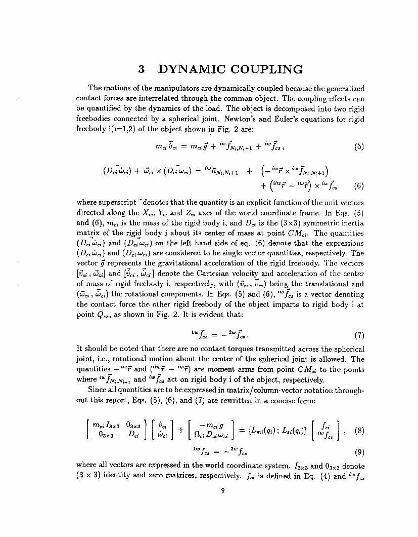
The motions of the manipulators are dynamically coupled because the generalized contact forces are interrelated through the common object. The coupling effects can be quantified by the dynamics of the load. The object is decomposed into two rigid freebodies connected by a spherical joint. Newton's and Euler's equations for rigid freebody i(i=1,2) of the object shown in Fig. 2 are:

where superscript 'denotes that the quantity is an explicit function of the unit vectors directed along the X,, Yw and 2, axes of the world coordinate frame. In Eqs. ( 5 ) and (6), m,; is the mass of the rigid body i, and D,; is the (3x3) symmetric inertia matrix of the rigid body i about its center of mass at point CM,;. The quantities (Dcicjci) and (Dciwci) on the left hand side of eq. ( 6 ) denote that the expressions (Dei &&) and (Dei w,i) are considered to be single vector quantities, respectively. The vector represents the gravitational acceleration of the rigid freebody. The vectors [i7& , &;I and [sei , sei] denote the Cartesian velocity and acceleration of the center of mass of rigid freebody i, respectively, with (Gk, .'ti) being the translational and ( Z c i , s,i) the rotational components. In Eqs. ( 5 ) and ( 6 ) ) iwfcs is a vector denoting the contact force the other rigid freebody of the object imparts to rigid body i at point Qu, as shown in Fig. 2. It is evident that:

4 -4

-+

(7) l w - 2w * f c s = - fa.

It should be noted that there are no contact torques transmitted across the spherical joint, i.e., rotational motion about the center of the spherical joint is allowed. The quantities -""F and (i'wF - '"3 are moment arms from point CM,; to the points where iWfN,,~I+l and

Since all quantities are to be expressed in matrix/column-vector notation through- out this report, Eqs. ( 5 ) , (6), and (7) are rewritten in a concise form:

4

act on rigid body i of the object, respectively.

where all vectors are expressed in the. world coordinate system. Isx, and 0 3 x 3 denote (3 x 3) identity and zero matrices, respectively. fci is defined in Eq. (4) and i w f c s

9

10

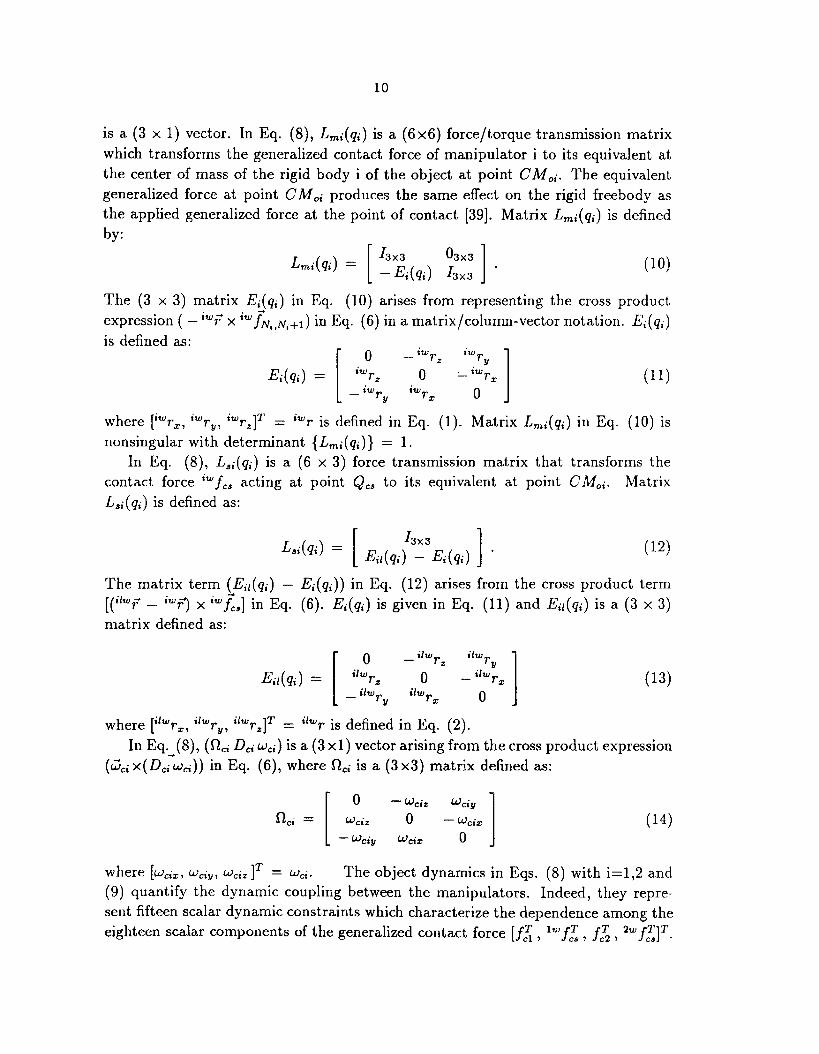
is a (3 x 1) vector. In Eq. ( S ) , L,;(q;) is a (6x6) force/torque transmission matrix which transforms the generalized contact force of manipulator i to its equivalent at the center of mass of the rigid body i of the object at point CM,;. The equivalent generalized force at point CM,i produces the same effect on the rigid freebody as the applied generalized force at the point of contact [39]. Matrix L,;(q;) is defined bv:

The (3 x 3) matrix Edq,) in Eq. (10) arises from representing the cross product expression ( - iwT x iw fN,,N,+*) in Eq. (6) in a matrix/column-vector notation. E;(q,) is defined as:

iw iw r z TY

Ei( q i ) = [ ;Gz -. 0 - i w r x ] (11) 0 iw

r y r x -

where [iwrx, iwrZ]T = iwr is defined in Eq. (1) . Matrix L,;(q;) in Eq. (10) is nonsingular with determinant { Lmi(q i )} = 1.

In Eq. (8), Lsi(qi) is a (6 x 3 ) force transmission matrix that transforms the contact force i w f c s acting at point Qcs to its equivalent at point CM,;. Matrix L,;(q;) is defined as:

The matrix term (Eil(q;) - E;(q;)) in Eq. (12) arises from the cross product term [ ( i lwF - '"3 x iwf7-b] in Eq. ( 6 ) . Ei(q,) is given in Eq. (11) and E;l(q;) is a (3 x 3) matrix defined as:

ilw ilw 0 - f z

E;&;) = 0 - (13) [ ilw rz 0

where [il'"rx, i lwry, ilwrZ]T = ilwr is defined in Eq. (2).

(& ;x (D&w&)) in Eq. (6), where Q, is a ( 3 x 3 ) matrix defined as: In Eq. ( S ) , (CL-i D k wn.) is a (3 x l ) vector arising from the cross product expression

where [Wcix, uny, WcizIT = w&. The object dynamics in Eqs. (8) with i=1,2 and (9) quantify the dynamic coupling between the manipulators. Indeed, they repre- sent fifteen scalar dynamic constraints which characterize the dependence among the eighteen scalar components of the generalized contact force [f:, '"f:, f;, *"f;J'.

11

They will be incorporated in the closed-chain dynamical equations. In addition to the dynamical constraints, the kinematic coupling between the manipulators also constrains the motion of the closed-chain mechanism. It is presented next.

4 KINEMATIC COUPLING

The manipulators are kinematically coupled because the ( N , + N 2 ) generalized coordinates (qT , qT)T are interrelated. The kinematic coupling effects can be quan- tified by equations showing the dependence among the generalized coordinates and their derivatives. These kinematic constraints can be determined by expressing the Cartesian translational velocity of the center of the spherical joint contained in the object in terms of the joint velocities of manipulator i(=l,2), and then obtaining a relationship among the generalized velocities.

The Cartesian translational velocity of the object at point Q,, and the object velocity a t point CM,; are related through the force transmission matrix L,i(qi). The relation among these velocities is:

where the (3 x 1) vector o, is the translational velocity of the center of the spherical joint in the world 'coordinates. Furthermore, the Cartesian velocities of rigid body i of the object at point CM,; and at the point of contact of the external forces imparted by manipulator i are related by:

[ vci ] = (LZt(qi))-l [ vi ] wci w;

where the (3x1) vectors q and w;(i=1,2) represent the translational and rotational velocities, respectively, of the end effector of manipulator i at its centerpoint in the world coordinates. A detailed derivation to obtain the result of Eqs. (15) and (16) based only on the geometry and kinematics of the closed-chain is provided in Appendix A. It is straightforward to verify by Eqs. (10) and (16) that w; = wc;,

since every point on the rigid end effector of manipulator i and the rigid body i of the complex object has the same Cartesian angular velocity in the world coordinate system. However, joint,

The velocities dinate frame and JiW(q;), that is:

it should be noticed that in general w,1 # wc2 due to the spherical

of the end effector of manipulator i in the Cartesian world coor- the joint space are related through the (6 x N;) Jacobian matrix

Eliminating [v:, wZlT from Eq. (15) using Eq. (16), and equating the right hand sides of the two sets of resulting equations obtained with i=1,2 give a relationship:

13

14

in which Eq. (17) has been applied. Equation (18) comprises three scalar constraint equations characterizing the kinematic dependence among the generalized velocities when the manipulators operate in the closed-chain configuration. Each independent scalar constraint contained in Eq. (18) causes the loss of one DOF in the closed-chain [34]. This is significant since the system DOF specifies the number of independent ways the multi-manipulator closed-chain can move without violating the constraints given by Eq. (18) [34]. The number of DOF for a three-dimensional kinematic chain mechanism consisting of rigid links serially connected by j1 single-DOF revolute joints and j 2 three-DOF spherical joints is determined by:

DOF = 6 ( k t o t - 1) - 5 j l - 3 j z (19)

where ktol is the total number of links(inc1uding a stationary, zeroth reference link the mechanism is mounted on). Equation (19) reflects the fact that each moving link has six DOF whereas the zeroth link has none, and each single-DOF joint causes a loss of five DOF for a moving link, while each three-DOF joint causes a loss of three DOF for a moving link. For the multi-manipulator configuration shown in Fig. 1, ktot = ( N I + N Z -t l), j1 = ( N , + N2), j , = 1, and the total sytem DOF is (N1 + N2 - 3) by Eq. (19). Indeed, the DOF for the closed-chain is equal to the number of generalized coordinates (q:, q;)T minus the number of independent scalar equations of constraint [34].

A dynamical model for the multiple manipulator system is presented next.

5 CLOSED-CHAIN MODEL IN JOINT SPACE

The dynamic constraints represented by Eqs. (8) with i=1,2 and (9) as well as the kinematic constraints in Eq. (18) must be satisfied during the closed-chain motion. The constraints may be combined with the equations of motion of the ma- nipulators to obtain a joint space dynamical model of the entire system. The model is formed by first combining the manipulator models and the dynamic constraints to obtain dynamical equations which contain explicitly an independent subset of the generalized contact forces. The dynamical equations are incorporated into the kine- matic constraints to obtain a functional relation for the generalized contact forces. These contact forces can then be eliminated from the equations of motion to obtain a closed-chain model for the entire system.

The dynamics of rigid body i of the object in Eq. (8) can be incorporated in the manipulator i model in Eq. (3) by the following two step procedure: (a) Eq. (8) is solved for fc; and (b) fcl is eliminated from Eq. (3) using the solution obtained in step (a). This procedure gives the composite dynamics for manipulator i and rigid body i of the object:

where A; is a ( 6 x 6 ) matrix:

It should be noted that Eq. (20) is an explicit function of the spherical joint contact force vector jwfCs which is defined in conjunction with Eqs. ( 5 ) - (7) and (9).

Since the closed-chain model is to be expressed in the joint space, the Cartesian variables w&, L& and 6,. of the object are eliminated from Eq. (20). The Cartesian acceleration of the object at point CM,; can be expressed in terms of the joint accelerations of manipulator i by differentiating Eq. (16) and applying Eq. (17):

( ~ f i ( q i ) ) - l [ j i w (ii + J i w ( q i ) i i ] (22)

where the (6 x 6 ) matrix (L:i)-l[= (O((L:i)-')/aqi)@;] and the (6 x N ; ) matrix j;w[= (aJ iw /aq i ) i i ] are functions of the joint positions and velocities of manipulator 1.

15

16

The closed-chain dynamics for the entire system are derived in two steps: (a) In- corporate Eqs. (16), (17) and (22) into Eq. (20) to obtain the composite manipulator i - rigid body i(of object) dynamics in the joint space; (b) The two sets of equations obtained from (a) with i=1,2 are combined and expressed in a concise form:

7 = D ( q ) $ + c(q, 4) + H A ( q , 4) f H B ( q , 4 ) 4 + A T ( ( ? ) 2 w f c 3 (23)

in which Eq. (9) has been used to eliminate l w f C 3 and where T = [I?', 27T]T

and q = [q: , q:lT are the joint torques and generalized coordinates for the entire system, respectively. The ( ( N , + N 2 ) x l ) vector C(q, 4) is defined as:

lh ((NI + N2) X (Ni + N2)) matrix D ( q ) is defined by:

where matrix 11, (i=1,2) in Eq. (25) is defined by Eq. (21). D ( q ) is the inertia matrix for the entire closed-chain system. It is symmetric, positive definite, and therefore nonsingular.

The ( (Nl+N2)xl) vector H A ( q , q ) and ( ( N l + N 2 ) x ( N l f N 2 ) ) matrix H R ( q , q ) in Eq. (23) are defined as:

H B ( q , 4) =

JL Kt A1 2 { (JL JK: I T } ONl x Nz [ O N ~ X N , J z T , L 3 2 & { ( J L G ) T } where $ { ( J L ~5,:)~) = [(i:,)-' J iw(q i ) + (L:i(qi))-' j i w ] with i=1,2 in Eq. (27).

matrix. It is defined by: The ( (Nl+N2) x3) matrix AT(q) in Eq. (23) is termed the contact force coefficient

17

The dynamics of both manipulators and mutually hdd object are represented in Eq. (23) as (N1 + N2) second order differential equations. Equation (23) contains ex- plicitly an independent subset of the generalized contact forces [fz, lW f;, fz, 2 w f 2 ] T acting on the object, namely 2wfCb. While Eq. (23) describes the dynamics of all components of the closed-chain, it does not account for the kinematic constraints be- tween the manipulators due to the common jointed load. To combine the kinematic constraints given by Eq. (18) and the closed-chain dynamics to obtain a model for the entire system, Eq. (18) is first expressed in a simplified, concise form in terms of the contact force coefficient matrix:

A(Q) Q = 0 3 x 1 (29) in which Eq. (28) has been applied. The corresponding acceleration constraints result from differentiating Eq. (29):

The ( 3 x ( N 1 +N2) ) matrix A[= (aA/aq)q] in Eq. (30) is a function of the generalized coordinates and velocities.

Equations (23) and (29) are derived independently based on the dynamics and kinematic constraints for the closed-chain, respectively. Matrix A(4) quantifies the coupling among the generalized velocities in Eq. (29). Interestingly, Eq. (23) reveals that AT(q) maps the three components of contact force acting at the center of the spherical joint in the object (*"fCs) to the joint space. A functional relation for the calculation of the object contact forces is obtained by solving Eq. (23) for the generalized accelerations and substituting the result in Eq. (30):

A D - 1 A T 2 w f c l = A q + A D - ' { r - C - HA - H B ~ } . (31)

Since A has rank three and D-' is positive definite and symmetric, then the (3x3) coefficient matrix ( A D-' AT) on the left hand side of Eq. (31) is positive definite, symmetric, and therefore nonsingular. Thus, the determination of 2w fcs using Eq. (31) is a well-specified problem. Interestingly, the object contact forces transmitted across the center of the spherical joint are functions of the generalized coordinates q, the generalized velocities 4, and the joint torques T using Eq. (31).

The dynamical model of the closed-chain system is determined by eliminating the vector ''"fts in Eq. (23) using Eq. (31). After rearranging, the resulting equations are:

A(q) (7 - C - H A - H B ~ } = Dij + A T ( A D - l A T ) - ' A 4 ( 3 2 )

where A(q) is a ( ( N I + N2) x (NI + N2)) matrix defined as:

18

Interestingly, matrix A(q) is idempotent, i.e., A(q) = A 2 ( q ) , and it is an orthogonal complement of the contact force coefficient matrix, i.e., A(q) AT(q) = O(Nl+Nz)x3.

Equation (32) represents a joint space rigid body dynamical model for the entire system in the Lagrange's formulation. It incorporates all constraint effects and con- tains (N1+ N z ) second order differential equations. The solution of Eq. (32) for the forward and inverse dynamics is discussed next.

5.1 Solving for Forward Dynamics

The joint torques T = ( I T * , 2rT)T over the specified time interval ( t o 5 t 5 t f ) are assumed to be given. The variables to be determined over the specified time interval are the ( N , + N 2 ) generalized coordinates q = (qT , q: )* and the ( N , + N2) generalized velocities q = (qT , 4jf)T, which are assumed to be given and to satisfy Eq. ( 2 9 ) at time to.

The closed-chain model in Eq. (32) contains (N1 + N2) second order differential equations and (Nl + N 2 ) generalized accelerations. Since matrix D ( q ) is nonsingular, Eq. (32) can be solved for the highest order derivative 4" and expressed as 2(N1 +N2) first order differential equations containing 2(N1 + N2) unknown variables ( q , q).

Since the number of first order differential equations is equal to the number of un- known scalar variables, the solution for the forward dynamics is well-specified when input T is known over the given time interval. Therefore the model given in Eq. (32) can be numerically integrated to provide dynamical simulation of the closed-chain mot ion.

5.2 Solving for Inverse Dynamics

The desired trajectories of the generalized coordinates and their derivatives: q , q , + over the specified time interval ( to 5 t 5 t j ) are assumed to be given which satisfy Eqs. (29) and (30). The variables to be determined over the specified time interval are the (Nl + N 2 ) joint torques T = ( T , T ) .

The closed-chain model in Eq. (32) involves (N1 + N2) second order differential equations containing (N1+ N2) joint torques. The rank of the (( N1 + N2) x (N1+ N2)) coefficient matrix A(q) defined in Eq. (33) which premultiplies vector T in the model determines the nature of the solution to the inverse dynamics. It is proven in Appendix B by analytical techniques that A(q) is a singular matrix and that its rank does not exceed the DOF of the closed-chain system, namely ( N l + N2 - 3). It should be mentioned that the proof in Appendix B requires knowledge of particular matrix- and vector-variables which are introduced in the next section(6). The proof that matrix A(q) is singular and that the runk(A(q) ) 5 ( N , + N2 - 3) is a new result for the case of two manipulators holding a spherically jointed payload. Therefore the problem of solving for the inverse dynamics is underspecified in nature. Equation (32)

1 T 2 T T

19

has infinitely many solutions for the joint torques when the generalized coordinates and their derivatives are known over the specified time interval.

The structure of the closed-chain joint space model given by Eq. (32) is not particularly suitable for the development of a control architecture, i.e., the joint torques cannot be solved by inverting matrix A(q), since it is singular. Furthermore, the number of scalar second order differential equations contained in Eq. (32) exceeds the DOF of the system. However, as shown in the next section, the joint space model is amenable to the realization of a reduced order model which is useful for controller design purposes.

6 REDUCED ORDER MODEL AND CONTACT FORCE DETERMINATION

The closed-chain system consisting of two serial-link manipulators containing N1 and N2 joints, respectively, mutually holding an object containing a spherical joint described by (N1 + N2) second order differential equations in Eq. (32) has (Nl + N2 - 3) DOF. The number of second order differential equations of motion is reduced from (Nl + N2) to (Nl + N2 - 3) in this section. The generalized contact forces are eliminated from the reduced order model, but can be calculated separately. The solution of the model for the unknown variables is discussed.

To determine a reduced order model, a new vector variable I/ = [VI, v2,. . . ? I / N , + N ~ - ~ ] * referred to as the pseudovelocity [1, 341 is introduced. The number of scalar components of v is equal to the DOF of the system. The pseudovelocity is defined by:

Y = B(q)Q. (34)

The ( ( N , + N2 - 3) x ( N l + N2) ) matrix B(q) in Eq. (34) is selected so that the composite ((Nl + N2) x ( N , + N 2 ) ) matrix ( AT(q) ; BT(q))T is nonsingular. It is convenient to partition the inverse of ( AT(q) ; BT(q))* into two matrices:

where II(q) is a ( ( N l +N2) x3) matrix and C(q) a ( (Nl +N2) x ( N , + N , -3)) matrix. Eq. (35) implies that A n = 1 3 x 3 , A x = 0(3X(Nl+N2-3)), B n = O ( ( N ~ + N Z - ~ ) X ~ ) ?

B = 1(N1+N2-3)X(N1+N2-3) and (n A + B , = I ( N ~ + N ~ ) X ( N ~ + N Z ) * The pseudovelocity emphasizes the fact that the linear combinations of the generalized velocities on the right hand side of Eq. (34) are not necessarily the time derivatives of any physical coordinates [l, 341. Indeed, the choice of matrix B(q) by the designer is somewhat arbitrary. Two examples of the selection of matrix B(q) given specific choices for the pseudovelocity vector Y by the designer are provided in Appendix C. Furthermore, the examples show that matrices U ( q ) and C(q) may be defined analyt- ically thus avoiding the numerical inversion of matrix (AT(q) ; B*(q))' for calculating their values.

Differentiating Eq. (34) establishes a relationship between the pseudo- and gen- eralized accelerations:

The ((NI + N2 - 3) x (NI + N2) ) matrix h[= (aB/aq)g] in Eq. (36) is a function of the generalized coordinates and velocities.

fi = Bf j + B q . (36)

Equations (29) and (34) can be solved for the generalized velocities:

q = C Y

21

(37)

22

in which Eq. (35) has been applied. Likewise, Eqs. (30) and (36) can be solved for the generalized accelerations:

4; = cri - [nA + C B ] C v . (38)

Substituting for q in Eq. (29) using Eq. (37) yields the kinematic veloc- ity constraint equation A C v = 03x1, which is identically true because A C = 0 ( 3 x ( ~ 1 + ~ 2 - 3 ) ) in accordance with Eq. (35). Thus the kinematic constraints are satisfied regardless of the values of the pseudovelocities; therefore, the closed-chain dynamics in Eq. (23) expressed in the pseudospace implicitly satisfy the kinematic constraints.

Premultiplying Eq. (23) by the matrix ET and utilizing the properties of Eq. (35) obtain:

ET D q = C T { t - C - HA - H B Q } . (39)

Substituting Eqs. (37) and (38) into Eq. (39) yields the reduced order equations of motion in the pseudospace:

ETDCri = ET { T + {D [IIA + Cb] - H B } Cv - C - H A } . (40)

Eq. (40) is comprised of ( N , + N2 - 3) second order differential equations, which is equal to the DOF of the entire system. It should be noted that the term ( A T 2 W f c s ) in Eq. (23) is implicitly cancelled in the reduced order model because ETAT = O ( ( N ~ + N ~ - ~ ) ~ ~ ) in accordance with Eq. (35). Thus, Eqs. (39) and (40) are not functions of the generalized contact forces which may be calculated in terms of the pseudovelocities using Eqs. (31) and (37):

f c S = A x v + AD-'{^ - c - H~ - H ~ c ~ ) . (41) A D - ~ A T 2w

It should be mentioned that 2wfcs can be calculated as a function of fi through premultiplying Eq. (23) by the matrix IIT and incorporating Eqs. (35), (37), and

It will be shown in the next section that the separated form of the model for the entire closed-chain system given by Eqs. (40) and (41) is useful for controller design purposes.

The solution of the reduced order model for the forward and inverse dynamics is now discussed.

(38)-

6.1 Solving for Forward Dynamics

The joint torques T = (l?, 2 ~ T ) T over the specified time interval ( t o 5 t 5 t,)

are assumed to be given. The variables to be determined over the specified time

23

interval are the (N1 + N2 - 3) pseudocoordinates p (= [pl, p a , . . . , p l ~ , + ~ , - 3 ] ~ } and the ( N I + N Z - 3) pseudovelocities v , where v = $. It is assumed that q and v are given at time to which satisfy Eq. (37).

The reduced order model in Eq. (40) involves (N1 + N2 - 3) second order dif- ferential equations containing (& + NZ - 3) pseudoaccelerations. Since matrix E* has full rank ( N , + N2 - 3 ) and matrix D(q) is positive definite and symmetric, then the square coefficient matrix ( C T D C ) in Eq. (40) is positive definite, symmetric, and therefore nonsingular. Thus Eq. (40) can be solved for the pseudoaccelera- tions and expressed as 2(N1 + N2 - 3) first order differential equations containing 2(N1 + N2 - 3) unknown variables ( p , v ) . Since the number of first order differential equations is equal to the number of unknown scalar variables, the solution for the forward dynamics is well-specified when the input T is known over the given time interval.

The reduced order model in Eq. (40) leads to a computationally efficient dynam- ical simulation of the closed-chain motion when compared to the joint space model given by Eq. (32). For example, with two six-joint manipulators (N1 = N2 = 6) holding a spherically jointed object, Eqs. (40) and (32) contain nine and twelve sec- ond order differential equations of motion, respectively. However, since the problem of analytically expressing the generalized coordinates q = (q: , qr)' in a reduced manner remains unsolved 11, 2 , 3, 71, Eqs. (40) and (41) are explicit functions of g

and not of the pseudocoordinate vector p . Thus it is nontrivial to numerically inte- grate the reduced order model. A method for circumventing this problem in discrete time which solves for the pseudocoordinates numerically is now discussed.

Let r denote the sampling period and assume that the joint torques ~ ( k r ) are given over the specified time interval k = Eo, ko + 1, . . . , kj, where time t = k I? and {ko, kj} are non-negative integers. The variables q and v are assumed to be given and to satisfy Eq. (37) at t = ko r. The nonsingular coefficient matrix (ET D E) on the left hand side of Eq. (40) is a function of g. The right hand side of Eq. (40) is a

function of the variables (q, v, 7 ) .

At the initial time Eq. (40) can be solved for the highest order derivative ($ (ko I')) and numerically integrated over the sampling period from t = KO I' t o t = (IC0 + 1) I' to obtain p ( t ) and v( t ) at t = (ko + 1) r. The drawback of the reduced order model being a function of the generalized coordinates is now evident. Indeed, q( (ko + 1) I?) must be determined before Eq. (40) can be solved for the highest order derivative ( 6 ( ( Lo + 1) r)) and numerically integrated from time t = ( ko + 1) I' to t = ( k0 + 2) I?. To solve this problem, Eq. (37) could be numerically integrated over the sampling period from t = ko I? to t = (ko + 1) I? to obtain q((k0 + 1) I?). This approach involves numerically integrating ( N , + N2) first order differential equations and is purely kinematical in nature.

Given (Q, Y, 7) at t = (ko + 1)r, the reduced order model can be solved for

24

(V((lC0 + 1) I?)) and numerically integrated to obtain p ( t ) and v( t ) at t = ( I C o + 2) I?. q ( t ) at 1 = (IC0 + 2)r can be obtained by integrating Eq. (37) from time t =

Continuing in the aforementioned manner, the dynamical, discrete time simula- (ko + i)r to t = (k0 + 2)r.

tion of Eq. (40) can be accomplished.

6.2 Solving for Inverse Dynamics

The desired trajectories of the generalized coordinates and their derivatives: q, q, q

over the specified time interval ( t o 5 t 5 t f ) are assumed to be given which satisfy Eqs. (29) and (30). The ( N l + N 2 ) scalar variables to be determined over the specified time interval are the joint torques 7 = (I?, 2 ~ T ) T .

The desired pseudospace trajectory (v, i) is first obtained by Eqs. (34) and (36) since the desired joint space variables and their derivatives are known. The reduced order model in Eq. (40) contains (Nl + N2 - 3) second order differential equations with (N1 + N , ) unknown joint torques. Moreover, the coefficient matrix ET which premultiplies T in Eq. (40) is rectangular with fewer rows than columns. Therefore, the solution to the inverse dynamics is underspecified, since the number of unknown joint torques exceeds the number of equations. Equation (40) has infinitely many solutions for T when the desired trajectories of the generalized coordinates and their derivatives are given over the specified time interval. A solution for the joint torques obtained from the reduced order model would not consider the spherical joint contact forces, which are governed by Eq. (41). In view of this a control architecture for the joint torques based on Eqs. (40) and (41) is derived in the next section.

7 CONTROL ARCHITECTURE

The problem considered is to derive a control law for the (N1+ N2) joint torques r = 2 ~ T ) T so that the force and position of the closed-chain mechanism behave in desirable manners. The controller is designed on the basis of the separated form of the closed-chain model given by Eqs. (40) and (41). Specifically, a control input T

is determined so that the pseudovariables (I/, fi} and the object contact forces 2w fc3

acting at the center of the spherical joint will be controlled separately. Finally, the modeling and control methodology presented here are compared to another model and control scheme recently proposed in the literature.

The controller consists of the sum of the outputs of a ( ( N , + N2) x 1) primary controller (TP) that is designed for cancellation of nonlinear terms in the model and a ( (N1 + N2) x 1) secondary controller ( r8) that performs closed-loop servoing. The composite control (7) is specified as T = TP + 7". r p is realized by introducing nonlinear feedback and/or feedforward loops into the closed-chain system such that the nonlinear terms in Eqs. (40) and (41) that are not explicit in the variables ('"f-, f i ) are cancelled. The primary controller is chosen as:

where the superscript A denotes that the quantity is estimated as a function of the desired(reference) feedforward trajectory (qref, v f c j ) and/or the feedback variables

(q , v). The composite control (T = r p + 7") is substituted into Eqs. (40) and (41). The resulting equations, under the assumption that the following relations hold:

can be expressed as:

i/ = ( c T D c ) - l C T P , (44)

2wfc, = ( A 0-1 AT)-' A D-1 r s (45) in which Eqs. (35) and (42) have been applied.

The design of the secondary controller (7.") is based on the structure of Eqs. (44) and (45) so as to obtain a closed-loop control system where the pseudovariables and object contact forces are servoed separately. The secondary controller is selected as:

rg = ATr; + Dkri (46)

25

26

where T: and T; are (3 x l ) and ( (N1+ N2 - 3) x l ) vectors, respectively, representing control variables to be determined. Substituting Eq. (46) into Eqs. (44) and (45), utilizing the matrix relations in Eq. (35), and rearranging give:

L; = 725, (47)

(48) where the assumption of perfect knowledge of the nonlinear terms in Eq. (43) has been applied.

Eqs. (47) and (48) represent the reduced order model equation (40) and the spherical joint contact force equation (41) in the closed-loop system, respectively. Suppose the secondary controller components 725 and 71" are feedback and/or feed- forward control laws selected by the designer to servo the pseudovariable error and the object contact force error, respectively. Since Eqs. (47) and (48) are completely decoupled, T: and 7; are independent, non-interacting controllers for the force- and position-control of the constrained multi-manipulator system, respectively. Thus, the force- and position-controlled DOF are decoupled when the composite control law (T = T P + 7") defined by Eqs. (42) and (46) is used in conjunction with Eqs. (40) and (41). This is a new result for the case of two manipulators holding a jointed object .

Interestingly, the structure of the composite controller (T = T P + T") reveals that it is a hybrid control strategy [32, 331. In the secondary controller defining Equation (46), the ( (Nl + N2) x3) matrix AT transforms the contact force controller 7: to the joint space. Likewise, the ((Nl + N,)x(Nl + N2 - 3)) matrix ( B e ) in Eq. (46) transforms the pseudovariable controller T; to the joint space. Therefore all (Nl + N2) actuated manipulator joints contribute to the force- and position-control of the entire closed-chain system.

In [9], the "orthogonal complement" C of the matrix A is defined by the equation A C = 03x9 for a pair of six-axis (N1 = N2 = 6) manipulators holding an object containing a spherical joint. A joint space reduced order model in the form of Eq. (39) is obtained by premultiplying the combined manipulator equations of motion by ET, which eliminates the generalized contact forces and reduces the number of

second order differential equations of motion from twelve to nine [9]. Eq. (39), however, contains (N1 + N2 - 3) second order differential equations of motion and (Nl + N2) generalized accelerations i. Thus the problem of solving Eq. (39) for q is underspecified and the reduced order model in the joint space is impractical for dynamical simulation. Eq. (39) also contains (N1 + N z ) joint torques T. An underspecified solution for the joint torques for position tracking is computed from the model in [9]. The approach used here additionally derives functional relations in Eqs. (31) and (41) for the generalized contact forces, which is not considered in the earlier work [9].

27

It is difficult to develop a control input r so as to decouple the joint space form of the reduced order model and contact force equation given by Eqs. (39) and (31), respectively. The advantage of introducing the pseudovariables (Y, b} and

determining matrices n and by Eq. (35) is that it becomes straightforward to derive a control architecture to completely decouple the reduced order model and contact force equation when they are expressed in the pseudospace by Eqs. (40) and (41), respectively.

CONCLUSION

The closed-chain motion of two manipulators holding an object containing a multiple-DOF spherical joint has been analyzed. A rigid body model was first devel- oped in the joint space. It includes the dynamics of all components of the closed-chain as well as the kinematic constraints. The system was transformed to obtain a reduced order model which also includes the dynamics of both manipulators and the object, but implicitly satisfies the kinematic constraints. Either form of the model more closely represents the physical behavior of the system than the model presented in [9], which includes the manipulator dynamics but does not include the dynamics of

the spherically jointed object. Furthermore, it has been shown that the solutions of the joint space and reduced order models for the forward dynamics are well-specified in nature, whereas their solutions for the inverse dynamics are underspecified.

In [9], the controller design was based only on the joint space reduced order model which contains no generalized contact forces. By considering both the reduced order model and separate contact force equation expressed in the pseudospace for the controller design, it has been shown here that the force- and position-controlled DOF can be completely decoupled. That is, the pseudovariables {v, c } and an independent subset of the generalized contact forces can be controlled independently using the proposed composite control architecture (7 = T P + 7") .

Derivation of an analytical expression for matrix B(q) which defines the pseu- dovelocity vector v is one of the main tasks when applying the reduced order model and control architecture to a specific application. Two examples of the selection of matrix B(q) such that matrix (A*(q) ; B*(q))* is nonsingular given specific choices of Y by the designer have been presented. Furthermore, the feasibility of analytically deriving matrices n(q) and C(q) to avoid numerically inverting (AT(q) ; BT(q>)T for calculating their values was investigated in the examples. In the previous work on two manipulators holding a rigid object [38, 391, matrix B(q) was presented only in general terms.

Each manipulator holding a rigid object was required to have N joints in [38, 391. The analysis in [9] was restricted to a pair of six-joint manipulators holding a spherically jointed object. The rigid body model and decoupled control architecture presented in this report are applicable to two manipulators containing N 1 and N2 joints, respectively.

The research presented in this report has uncovered and identified a wealth of open problems and issues associated with the closed-chain motion of two manipu- lators holding a spherically jointed object that warrant future attention. The total DOF in the closed-chain system is ( N , + Nz - 3) as discussed in section 4. When there are redundant DOF in the system, i.e., when the total DOF of the closed-chain system exceeds nine, the choice for and the physical interpretation of the additional

29

30

pseudovelocities [ulo, yl,. . . , U N ~ + N ~ - ~ ] ~ need to be investigated. This includes the development of criteria or analytical methods for selecting the matrix B( q).

Another interesting suggested future work area involves using the rigid body model and proposed controller to investigate properties of the closed-loop system in the presence of force disturbances, or uncertainty in the knowledge of the system dynamics and/or the kinematic constraints.

Slippage and friction were not considered in this report, but are important factors in the modeling and control of two interacting manipulators. It would be helpful and desirable to determine if the results presented here could be extended to include these effects.

The approach to the problem discussed here for the spherically jointed payload case could be applied to other interacting manipulator problems, e.g., two or more manipulators holding other complex jointed payloads such as an object containing a

universal joint.

9 ACKNOWLEDGEMENT

This research was supported by the Office of Engineering Research Program, Basic Energy Sciences, of the U.S. Department of Energy under Contract No. DE- AC05-840R21400 with Martin Marietta Energy Systems, Inc.

V. Protopopescu, Dr. J. Jansen, and Dr. R. Kress for reviewing this report and providing many insightful suggestions for its improvement.

The author wishes to express his sincere thanks to Dr.

31

References

111 Raimo K. Kankaanranta and Heikki N. Koivo, Tampere University of Technol- ogy, Tampere, Finland, "Dynamics and Simulation of Compliant Motion of a Manipulator," IEEE Journal of Robotics and Automation, April 1988, vol. 4, no. 2, pp. 163-173.

[2] Raimo K. Kankaanranta and Heikki N. Koivo, Tampere University of Tech- nology, Tampere, Finland, " Stability Analysis of Position-Force Control Using Linearized Cartesian Space Model," International Federation of Automatic Con- trol(IFAC) Symposium on Robot Control, Karlsruhe, Germany, October 5-7, 1988, pp. 95.1-95.6.

131 N.H. McClamroch and D. Wang, "Feedback Stabilization and Tracking of Con- strained Robots," IEEE Transactions on Automatic Control, May 1988, vol. 33, no. 5, pp. 419-426.

[4] Raimo K. Kankaanranta and Heikki N. Koivo, Tampere University of Tech- nology, Tampere, Finland, "A Model for Constrained Motion of a Serial Link Manipulator," IEEE International Conference on Robotics and Automation, San Francisco, CA, April 1986, vol. 2, pp. 1186-1190.

[5] A.A. Cole, "Control of Robot Manipulators with Constrained Motion," 28th Conference on Decision and Control, Tampa, FL, USA, December 1989, pp.

1657-1658.

[6] J.K. Mills and A.A. Goldenberg, "Force and Position Control of Manipulators During Constrained Motion Tasks," IEEE Transactions on Robotics and Au- tomation, February 1989, vol. 5 , no. 1, pp. 30-46.

[7] N.H. McClamroch, "Singular Systems of Differential Equations as Dynamic Models for Constrained Robot Systems," IEEE International Conference on Robotics and Automation, San Francisco, CA, USA, April 1986, vol. 1, pp. 21- 28.

[8] H. Huang, "The Unified Formulation of Constrained Robot Systems," IEEE International Conference on Robotics and Automation, Philadelphia, PA, USA, April 1988, vol. 3, pp. 1590-1592.

[9] J.Y.S. Luh and Y.F. Zheng, "Constrained Relations Between Two Coordinated Industrial Robots For Motion Control," International Journal of Robotics Re- search, Fall 1987, vol. 6, no. 3, pp. 60-70.

33

34

[lo] K.I. Kim and Y.F. Zheng, "TWO Strategies of Position and Force Control for Two Industrial Robots Holding a Single Object ," Robotics and Autonomous Systems, December 1989, vol. 5, no. 4, pp. 395-403.

[ll] J.M. Tao, J.Y.S. Luh, and Y.F. Zheng, "Compliant Coordination Control of Two Moving Industrial Robots," IEEE Transactions on Robotics and Automation, June 1990, vol. 6, no. 3, pp. 322-330.

[12] Y.F. Zheng and J.Y.S. Luh, "Optimal Load Distribution for Two Industrial Robots Handling a Single Object," IEEE International Conference on Robotics and Automation, Philadelphia, PA, USA, April 1988, vol. 1, pp. 344-349.

[13] Y. Nakanura, K. Nagai, and T. Yoshikawa, "Dynamics and Stability in Coor- dination of Multiple Robotic Mechanisms," International Journal of Robotics Research, April 1989, vol. 8, no. 2, pp. 44-61.

[14] D.E. Orin and S.Y. Oh, "Control of Force Distribution in Robotic Mechanisms Containing Closed Kinematic Chains," ASME Journal of Dynamic Systems, Measumment, and Control, June 1981, vol. 102, pp. 134-141.

[15] K. Laroussi, H. Hemarni, and R.E. Goddard, "Coordination of Two Planar Robots in Lifting," IEEE Journal of Robotics and Automation, February 1988, vol. 4, no. 1, pp. 77-85.

[16] B.S. Ryuh and G.R. Pennock, "Dynamic Formulation for Multiple Cooperating Robots Forming Closed Kinematic Chains," Proceedings IASTED International Symposium Robotics and Automation, Santa Barbara, CA, USA, May 1988, pp. 64-68.

[17] R.A. Freeman, "Dynamic Modeling of Robotic Linkage Systems in Terms of Arbitrary Sets of Generalized Coordinates," IEEE International Conference on Systems, Man, and Cybernetics, Alexandria, VA, October 1987, USA, vol. 2, pp. 787-797.

[18] I.D. Walker, S.I. Marcus, and R.A. Freeman, "Distribution of Dynamic Loads for Multiple Cooperating Robot Manipulators," Journal of Robotic Systems, January 1989, vol. 6, no. 1, pp. 35-47.

[I91 K. Kreutz and A. Lokshin, "Load Balancing and Closed Chain Multiple Arm Control," American Control Conference, Atlanta, GA, USA, June 1988, vol. 3, pp. 2148-2155.

(201 J.T. Wen and K. Kreutz, "Stability Analysis of Multiple Rigid Robot Manip- ulators Holding a Common Rigid Object," 27th Conference on Decision and Control, Austin, TX, USA, December 1988, vol. 1, pp. 192-197.

35

[21] J.T. Wen and K. Kreutz, "Motion and Force Control For Multiple Cooperative Manipulators," IEEE International Conjerence on Robotics and Automation, Scottsdale, AZ, USA, May 1989, vol. 2, pp. 1246-1251.

[22] M.E. Pittelkau, "Adaptive Load Sharing Force Control for Two-Arm Manipu- lators,,, IEEE Internationul Conference on Robotics and Automation, Philadel- phia, PA, USA, April 1988, vol. 1, pp. 498-503.

[23] S.A. Hayati, "Position and Force Control of Coordinated Multiple Arms," IEEE Tmnsactions on Aerospace and Electronic Systems, September 1988, vol. 24, no. 5, pp. 584-590.

[24] S.A. Hayati, K.S. Tao, and T.S. Lee, "Dual Arm Coordination and Control," Robotics and Autonomous Systems, December 1989, vol. 5, no. 4, pp. 333-344.

[25] C.R. Carignan and D.L. Akin, "Cooperative Control of Two Arms in the Trans- port of an Inertial Load in Zero Gravity," IEEE Journal of Robotics and Au- tomation, August 1988, vol. 4, no. 4, pp. 414-419.

[26] C.R. Carignan and D.L. Akin, "Optimal Force Distribution for Payload Using a Planar Dual- Arm Robot," ASME Journal of Dynamic Systems, Measurement, and Control, June 1989, vol. 111, pp. 205-210.

[27] C.R. Carignan, "Adaptive Tracking for Complex Systems Using Reduced Order Models," IEEE International Conference on Robotics and Automation, Cincin- nati, OH, USA, May 1990, vol. 3, pp. 2078-2083.

[28] 0. Khatib, "Object Manipulation in a Multi-Effector Robot System," 4th In- ternational Symposkum on Robotics Research, University of California at Santa Cruz, 1987, MIT Press Series on Artificial Intelligence, edited by R. Bolles and B. Roth, pp. 137-144.

[29] T.J. Tarn, A.K. Bejczy, and X. Yun, "New Nonlinear Control Algorithms for Multiple Robot Arms," IEEE Tmnsactions on Aerospace and Electronic Sys- tems, September 1988, vol. 24, no. 5, pp. 571-583.

1301 T.E. Alberts and D.I. Soloway, "Force Control of a Multi-Arm Robot System," IEEE International Conference on Robotics and Automation, Philadelphia, PA, USA, April 1988, vol. 3, pp. 1490-1496.

[31] S.A. Schneider and R.H. Cannon, Jr., "Object Impedance Control for Coop- erative Manipulation: Theory and Experimental Results," IEEE International Conference on Robotics and Automation, Scottsdale, AZ, USA, May 1989, vol. 2, pp. 1076-1083.

36

[32] J. J. Craig, Introduction to Robotics, Mechanics and Control, Addison-Wesley Publishing Co., 2nd edition, 1989, chap. 11.

[33] D.E. Whitney, "Historical Perspective and State of the Art in Robot Force Control," International Journal of Robotics Research, vol. 6, no. 1, pp. 3-14, Spring 1987.

[34] F.R. Gantmacher, Lectures in AnaZytical Mechanics, USSR: Mir Publishers, 1975.

[35] F.R. Gantmacher, The Theory of Matrices, Vol. 1, Chelsea Publishers, 1960.

I361 K.S. Symon, Mechanics, Addison-Wesley, 1953.

[37] C.R. Weisbin, B.L. Burks, J.R. Einstein, R.R. Feezell, W.W. Manges, and D.H. Thompson, "HERMIES-111: A Step Toward Autonomous Mobility, Manipula- tion and Perception," Robotica, vol. 8, part 1 , January-March 1990, pp. 7-12.

[38] M.A. Unseren and A.J. Koivo, "Reduced Order Model and Decoupled Control Architecture for Two Manipulators Holding an Object," Student paper pre- sented at IEEE International Confemnce on Robotics and Automation, Scotts- dale, AZ, USA, May 1989, vol. 2, pp. 1240-1245.

[39] M.A. Unseren, "Modeling and Control of Two Cooperating Manipulators for Assembly Tasks," PhD Thesis, School of Electrical Engineering, Purdue IJni- versity, West Lafayette, Indiana, USA, August 1989.

[40] M.A. Unseren, "A Rigid Body Model and Decoupled Control Architecture for Two Manipulators Holding a Complex Object," To Appear in Computers and Electrical Engineering, (1991).

APPENDIX A

RELATIONSHIP AMONG THE CARTESIAN VELOCITIES FOR THE RIGID BODY i OF

THE COMPLEX OBJECT AT THE CENTER OF MASS AND AT THE CONTACT POINTS

The Cartesian velocity relations given by Eqs. (15) and (16) are derived in this Appendix based on the geometry and kinematics of the closed-chain. The trans- lational velocity vector vc; defined in conjunction with Eq. ( 5 ) can be derived as

follows :

( A 4 v,; = - { iN, Pw (!?*I + * w + A ) }

dt

Similarly, the translational velocity vector vcs defined in conjunction with Eq. (15) can be derived as follows:

where ;p:(q;) in Eqs. (A. l ) and (A.2) is a (3 x 1) vector emanating from the origin of the ( X w , Yw, Z w ) world coordinate frame to the origin of the ( X i ! , Y$), Zi!) coordinate frame. Thus 'p$ ( P i ) represents the Cartesian translational position of the centerpoint of the end effector for manipulator i in the world coordinate system. The translational velocity vector v; defined in conjunction with Eq. (16) is related to vector ' p > ( q ; ) as foHows:

In Eqs. (A. l ) and (A.2), $(iwr(q;)) and $(ilwr(q;)) denote the time derivatives of vectors iwr(gi) and 'lWr(g;), respectively, with reference to the world coordinate

vectors '"r(q;) and i""r(q;), respectively, with reference to the end effector coordinate system (Xg! , YZ), Z i ! ) . Then the following relationships hold [36]:

system ( X w , Yw, Zw). Let zit( d* iw r(qi)) and s ( i ' w T ( q j ) ) denote the time derivatives of

ilw ilw 0 - r z rv rx 0 - T X

rY rX

ilw ilw

0 ilw ilw - W ; (A.5)

37

38

where the last term on the right hand side of Eq. (A.4) arises from representing the cross product expression (b; x iwF(q;)) [ = - iwF(q;) x w";] in a matrix/column-vector notation. Likewise, the last term on the right hand side of Eq. (A.5) arises from the cross product expression (3; x "".'(q;)).

Manipulator i securely holds the rigid body i of the complex object without slippage. Moreover, the (Xi!, Y l ) , 2:;) coordinate frame shown in Fig. 1 moves as the end effector for manipulator i moves. Points CM,; and Q,,, which coincide with the tails of vectors (;r, 'wr(q;)) and ("r, ""r(q;)) respectively, as shown in Fig. 2, are stationary with respect to the (Xi!, Y$), 2;:) coordinate frame. Furthermore, there is no joint variable associated with the local end effector coordinate frame. That is, the outermost scalar joint variable qiN, for manipulator i contained in the vector q; = [ q i l , q ; ~ , coordinate frame. Therefore vectors (;T, 'wr(q;)p "r , alwr(q;)) are constant(stationary) with respect to the ( X i ! , Y$), ZE!) coordinate frame. The time derivatives of vectors iwr(qi) and ""r(q,) with respect to the local moving coordinate frame are given by:

- . , q ; N , l T is associated with the (Xi!-,, Y$L1,

Incorporating Eqs. (A.3), (A.4) and (A.6) into Eq. ( A . l ) yields the following relation :

iw 0 - v,; = 0; -

Similarly, Eqs. (A.3), (A.5) ana (A.7) are substituted into Eq. (A.2):

if w ilw r z f Y

v,, = 0; - [ - 0 - ilWrz ] w; . 0 ilw

f X TY -

Equations (A.8) and (A.9) can be expressed in concise forms:

(A.10)

(A.11)

in which Eqs. (11) and (13) have been applied, respectively.

39

As discussed in Section 4, every point on the rigid body i of the shared payload and on the end effector of manipulator i has the same Cartesian angular velocity in the world coordinates. Thus the following relation holds:

W d = W i . (A.12)

Equations (A.lO) and (A.12) can be combined and expressed in terms of the force/ torque transmission matrix L,; (q i ) :

[ vn. ] = (LLl(q;))-* [ ] W d wi

(A.13)

in

in

which Eq. (10) has been applied. Equation (A.13) is in agreement with Eq. (16). Eliminating [v:, wTIT from Eq. (A . l l ) using Eq. (A.13) gives a relationship:

Substituting for Lz i (q ; ) in Eq. (A.14) using Eq. (10) and simplifying yield:

vca = [ ~ s x J ; E i ( q i ) - ~ i l ( q i ) l [ ] Wci

Finally, Eq. (A.15) can be expressed in a compact form:

which Eq. (12) has been applied. Eauation (A.16) is in agreement with Ea. (151.

(A.15)

(A.16)

APPENDIX 13

PROVING SINGULARITY OF THE JOINT TORQUE COEFFICIENT MATRIX

In this Appendix it will be proven that matrix A(q) which premultiplies the vector of joint torques in Eq. (32) has less that full rank and thus is singular. The definition of the pseudovelocity vector Y given in Eq. (34), the matrix relations given by Eq. (35), and the definition of A(q) in Eq. (33) will be used in evaluating the rank of A(q). Additionally, the following matrix property will be used. Suppose two (n x n) real matrices X and Y are given. Matrix X is assumed to possess full rank n and thus is nonsingular. Then the following mathematical relation applies [35]:

rank(Y) = r a n k ( X Y ) = r a n k ( Y X ) = rank(X*Y) = ranlc(YXT). (B.l)

The rank of ACq) may now be determined. By the property of Eq. (B.l), the following relation holds:

ranE(A) = rank { [ ET] A [ A T ; q} . The rank of the ( ( N l + I V 2 ) x ( N l + N z ) ) matrix within the braces on the right hand side of Eq. (B.2) is now analyzed by first decomposing it into four submatrices:

The submatrices can be expanded by replacing A with the right hand side of Eq. (33) and simplified by invoking the matrix relations in Eq. (35). Indeed, it is straightforward to verify that:

Equation (B.4) reveals that the first three columns of the matrix ([H ; E]* A [AT ; BT]) contain all zeros. Thus the matrix ([n ; E]' A [A* ; BT]) is singular. Furthermore, the runk([II; ZIT A [AT ; BT]) I (NI + NZ - 3).

Since matrix ([TI; E]' A [A*; B']) is singular, then matrix A is also singular with runk(A) _< (N1 + N2 -3) because the ranks of these two matrices are the same as shown in Eq. (B.2). Interestingly, this result indicates that the rank of A(q) does not exceed the DOF of the closed-chain configuration, namely (Nl + N2 - 3) .

41

APPENDIX C

SPECIFICATION OF ANALYTICAL FORMS FOR MATRICES B(q), n(q), AND C(q)

In this Appendix two examples of the selection of matrix B(q) which defines the pseudovelocity vector u in accordance with Eq. (34) are provided given specific choices for v by the designer. Additionally, the analytical derivation of matrices n(q) and C(q), which are defined by Eq. (35), is presented. The case of two six-axis (N1 = N2 = 6) manipulators holding a spherically jointed object is considered in the examples. It is assumed that the (6 x 6) Jacobian matrix J;,(q;) for manipulator i(=1,2) defined in conjunction with Eq. (17) possesses full rank six and thus is non- singular. In this case the closed-chain system has nine DOF and the pseudovelocity vector v contains nine scalar components, i.e., I/ = [ul, u2, . . . , v9IT.

The definition of matrix A(q) given by Eqs. (28) and (29) is repeated here for

convenience:

4) = [m?l) (G1k1)I-l Jlw(al1; - G ( q 2 ) (~T,2(cr2) ) - ' J 2 d d - J - (C.1)

Example 1 : In this example the pseudovelocities are chosen to be the Cartesian angular velocities of rigid body 2 of the complex object as well as the Cartesian velocities of the center of mass of rigid body l(of the object) at point CMOl, i.e., Y = [us, v z , Suppose the first three pseudovelocities [VI, v2, v3]* are expressed in terms of the joint velocities of manipulator 2 while the last six pseudovelocities are in terms of the joint velocities of manipulator 1. In this case the (9 x 12) matrix B(q) is selected as:

03x6 103x3; 13x3 I J ~ w ( q 2 )

(E, (Q1) JlW(Q1) 06x6

in which Eqs. (lo), (16), and (17) have been used.

with (N1 = IV, = 6) is presented here in a partitioned form: The (12 x 12) composite matrix ( A T ( q ) ; BT(q))T defined by Eqs. (C.1) and (C.2)

where the (6 x 6) matrices q ( q 1 ) and G(q2) in Eq. (C.3) are defined s:

4 3

44

Matrix (AT(q) ; BT(q))T given by Eq. (C.3) must be nonsingular in accordance with Eq. (35). The determinant of this composite matrix is given by [35]:

where det [ ] denotes the determinant of [ 1. To determine the rank of (AT(q) ; BT(q))T, the rank of matrix Q ( q 2 ) contained on the right hand side of Eq. (C.6) is needed. @ ( q 2 ) can be simplified by incorporating Eqs. (10) and (12) with i=2 into Eq. (C.5) and rearranging:

(C.7)

Interestingly, Eq. (C.7) reveals that matrix @ ( q 2 ) is nonsingular and that it satisfies the relation: (@(q2))2 = 16x6. Given that Jiw(qi) and Lmi(q i ) , i=1,2, are nonsingular matrices, the application of the matrix relation given by Eq. (B.l) to the matrix product terms contained on the right hand side of Eq. (C.6) reveals that matrix (AT(q) ; BT(q))T is nonsingular.

Matrix ( A T ( q ) ; BT(q))T in Eq. (C.3) can be symbolically inverted using the method of partitioning [35]:

The (12 x 3) matrix H(q) and the (12 x 9) matrix C(q) defined by Eq. (35) with (Nl = N2 = 6) are comprised of the first three and last nine columns, respectively, of the matrix contained on the right hand side of Eq. (C.8):

in which Eq. (C.7) has been applied. It is straightforward to verify that matrices

A(q), B(q) , n(q), and C(q) defined by Eqs. (C.l), (C.2), (C.9), and (C.10) respec- tively, satisfy the matrix relations given in Eq. (35) with ( N , = N2 = 6).

45

B(q) =

Example 2 : In this example the pseudovelocities are chosen to be the Cartesian angular velocities of the two rigid bodies comprising the common load as well as the Cartesian translational velocities of the center of the spherical joint at point QcJ, i.e., v = [uz, v:, u:IT. Suppose the first three pseudovelocities [VI, v2, u3IT

are expressed in terms of the joint velocities of manipulator 2 while the last six pseudovelocities are in terms of the joint velocities of manipulator 1. In this case the (9 x 12) matrix B(q) is selected as:

- O3x6 [ 0 3 x 3 ; 1 3 x 3 1 J z w ( q 2 ) -

L:l(41) V J : l ( q w Jl&d 0 3 x 6

- [ 0 3 x 3 ; 13x3 I Jlw(q1) 0 3 x 6 +

(C.11)

where the (6 x 6) matrices Q(q1) and d i ( q 2 ) in Eq. (C.12) are specified in Eqs. ((2.4) and (C.7), respectively. The (6 x 6) matrix X(q1) in Eq. (C.12) is defined as:

(C.13)

Matrix (A*(q) ; BT(q))T given by Eq. (C.12) must be nonsingular in accordance with Eq. (35). The determinant of this composite matrix is given by [35]:

To determine the rank of (AT(q); BT(q))T, the rank of matrix X ( q 1 ) contained on the right hand side of Eq. ((2.14) is needed. A ( q 1 ) can be simplified by incorporating Eqs. (10) and (12) with i=l into Eq. (C.13) and rearranging:

(C.15)

Equation (C.15) reveals that A(ql ) is nonsingular and det [X(ql)] = 1. Given that JiW(q.;) and Lmi(qi), i=1,2, and ( a ( q 2 ) are nonsingular matrices, the application of the matrix relation given by Eq. (B.l) to the matrix product terms contained on the right hand side of Eq. ((2.14) reveals that matrix (AT(q) ; BT(q))T is nonsingular.

46

Matrix (AT(q) ; B’(q))T in Eq. (C.12) can be symbolically inverted using the method of partitioning [35]:

(C.16) The (12 x 3) matrix n(q) and the (12 x 9) matrix C(q) defined by Eq. (35) with

(N1 = N2 = 6) are comprised of the first three and last nine columns, respectively, of the matrix contained on the right hand side of Eq. (C.16):

1 06x3 c (C.17)

1 0 6 x 3 J a q d (%))-l

V q ) = - J&?Z) %z) W l 1 ) (J?211(ql))-1 ( W I W

(C.18)

in which Eq. (C.7) has been used. It is straightforward to verify that matrices A(q) , B(q) , n(q), and C(q) defined by Eqs. (C.l), (C.ll) , (C.17), and ((2.18) re- spectively, satisfy the matrix relations given in Eq. (35) with (N, = Nz = 6).

ORNL/TM-11752 CESAR-91/01

INTERNAL DISTRIBUTION

1. B. R. Appleton 2. J. E. Baker 3. A. L. Bangs 4. M. Beckerman 5. J. R. Einstein 6. K. Fhjimura 7. J. F. Jansen 8. J. P. Jones 9. H. E. Knee

10. R. L. Kress 11. R. C. Mann 12. E. M. Oblow

18. V. Protopopescu 13-17. F. G. Pin

19. D. B. Reister 20. P. F. Spelt 21. F. J. Sweeney

22-26. M. A. Unseren 27. R. C. Ward 28. EP&MD Reports Office

29-30. Laboratory Records Department

31. Laboratory Records,

32. Document Reference

33. Central Research Library 34. ORNL Patent Section

ORNL-RC

Section

EXTERNAL DISTRIBUTION

35. Office of Assistant Manager, Energy Research and Development, Department of Energy, Oak Fiidge Operations, Oak Ridge, T N 37831

36, Dr. Peter Allen, Department of Computer Science, 450 Computer Science, Columbia University, New York, NY 10027

37. Dr. Wayne Book, Department of Mechanical Engineering, J. S. Coon Building, Room 306, Georgia Institute of Technology, Atlanta, GA 30332

38. Prof. John J. Dorning, Department of Nuclear Engineering and Physics, Thornton Hall, McCormick Rd., University of Virginia, Charlottesville, VA 22901

39. Dr. Steven Dubowsky, Massachusetts Institute of Technology, Building 3, Room 469A, 77 Massachusetts Ave., Cambridge, MA 02139

40. J. Duffy, Director, Center for Intelligent Machines and Robotics, University of Florida, 300 Meb, Gainesville, FL 32611

41. Dr. Avi Kak, Robot Vision Lab, Department of Electrical Engineering, Purdue University, Northwestern Ave., Engineering Mall, West Lafayette, IN 47907

42. Dr. James E. L e k , 13013 Chestnut Oak Dr., Gaithersburg, MD 20878 43. Dr. Oscar P. Manley, Division of Engineering, Mathematical, and

Geosciences, Office of Basic Energy Sciences, ER-15, U.S. Department of Energy - Germantown, Washington, DC 20545

44. Prof. Neville Moray, Department of Mechanical and Industrial Engineering, University of Illinois, 1206 West Green St., Urbana, IL 61801

45. Dr. Wes Snyder, Department of Radiolggy, Bowman Gray School of Medicine, 3005 Hawthorne Dr., Winston-Salem, NC 27103

46. D. Tesar, Department of Mechanical Engineering, University of Texas, 26 San Jacinto, Austin, TX 78712

47. Prof. Mary F. Wheeler, Rice University, Department of Mathematical Sciences, P.O. Box 1892, Houston, TX 77251

48-57. Technical Information Center, P.O. Box 62, Oak Ridge, T N 37831

47