aerospace

Review

A Review on Gas Turbine Gas-Path Diagnostics:State-of-the-Art Methods, Challenges and Opportunities

Amare D. Fentaye 1, Aklilu T. Baheta 1, Syed I. Gilani 1 and Konstantinos G. Kyprianidis 2,*1 Mechanical Engineering Department, Universiti Teknologi PETRONAS, Tronoh 32610, Malaysia2 School of Business, Society and Engineering, Mälardalen University, 883, SE-72123 Västerås, Sweden* Correspondence: konstantinos.kyprianidis@mdh.se

Received: 12 June 2019; Accepted: 14 July 2019; Published: 23 July 2019�����������������

Abstract: Gas-path diagnostics is an essential part of gas turbine (GT) condition-based maintenance(CBM). There exists extensive literature on GT gas-path diagnostics and a variety of methods havebeen introduced. The fundamental limitations of the conventional methods such as the inability todeal with the nonlinear engine behavior, measurement uncertainty, simultaneous faults, and thelimited number of sensors available remain the driving force for exploring more advanced techniques.This review aims to provide a critical survey of the existing literature produced in the area over thepast few decades. In the first section, the issue of GT degradation is addressed, aiming to identify thetype of physical faults that degrade a gas turbine performance, which gas-path faults contribute moresignificantly to the overall performance loss, and which specific components often encounter thesefaults. A brief overview is then given about the inconsistencies in the literature on gas-path diagnosticsfollowed by a discussion of the various challenges against successful gas-path diagnostics and themajor desirable characteristics that an advanced fault diagnostic technique should ideally possess.At this point, the available fault diagnostic methods are thoroughly reviewed, and their strengthsand weaknesses summarized. Artificial intelligence (AI) based and hybrid diagnostic methods havereceived a great deal of attention due to their promising potentials to address the above-mentionedlimitations along with providing accurate diagnostic results. Moreover, the available validationtechniques that system developers used in the past to evaluate the performance of their proposeddiagnostic algorithms are discussed. Finally, concluding remarks and recommendations for furtherinvestigations are provided.

Keywords: gas turbine performance; gas-path diagnostics; condition-based maintenance; fault diagnosticmethods; diagnostic method validation

1. Introduction

In today’s competitive business world, one way to increase profitability of machinery equipmentor a process plant is to reduce its operational and maintenance expenses while increasing productivity.Gas turbine (GT) is one of the most expensive devices in aircraft and industrial applications,where reliability and availability are the two most desirable attributes. In the past several decades,trillions of dollars was invested globally in the operation and maintenance of GTs [1,2]. However,due to their rising roles in the fast-growing industry, the market trend is still expected to be continuedinto the foreseeable future. According to the International Air Transport Association (IATA) report,in 2014, the world fleet count was 24,597 aircrafts. In this fiscal year, globally, airlines spent $62.1billion on Maintenance, Repair, and Overhaul (MRO), of which about 40% was for engine maintenance.In 2024, the engines MRO is expected to reach over $36 billion, with a 3.8% increasing rate perannum [3]. One can see how large these expenses would be if they are extended to include all types ofGT applications. Studies on the GT market indicated that the market for other engine groups is much

Aerospace 2019, 6, 83; doi:10.3390/aerospace6070083 www.mdpi.com/journal/aerospace

Aerospace 2019, 6, 83 2 of 53

bigger than the aircraft engines due to rapid industrialization across the globe and the rising demandfor power generation, mechanical drives and propulsion [2,4–6].

The GT fuel consumption and the likely increase in fuel price is another critical issue. For example,the US Department of Defense (DOD) alone consumes 4.6 billion gallons of fuel annually, which is93% of the US government fuel consumption and the 34th largest fuel consumption in the world,of which about 85% is for Air Force and Navy uses [7,8]. On the other hand, in combined cycle powerplants (CCPPs), the fuel cost covers 75% of the total life-cycle cost (LCC) [6]. Therefore, operating theGT as close to its clean conditions as possible may have a significant contribution to reducing theengine operating expenses. This can be achieved via an improved maintenance policy assisted by moreadvanced engine health monitoring (EHM) systems [9].

The gas turbine maintenance and operation costs are highly influenced by the performanceof the engine. Engine overall performance relies on the performance of the gas-path components(mainly the compressor(s) and turbine(s)) and these components are major problem areas due to theirexposure to different internal and external degradation causes [10]. Some of the major and mostlikely existing problems are drop in compressor efficiency due to fouling or erosion or object damage,loss in turbine efficiency due to blade erosion and blade creep with subsequent tip of probe andshroud damage, decrease in air flow capacity due to fouling, and an increase in flow capacity due toturbine erosion. However, these faults are not directly measurable. The gas-path diagnostic technologythus analyses the engine performance and identifies potential faults and provides an early warningbefore these faults develop into more complex problems. An effective and reliable gas-path diagnostictool that could detect, isolate, and assess potential problems, based on the measurement deviations,and suggest solutions well before they develop into more complex problems is therefore very essential.This plays a major role in the investment by ensuring high levels of GT reliability and availabilityalong with its best operating performance. There have been a variety of gas path diagnostic methodsintroduced so far beginning with the traditional model-based (MB) methods (such as Kalman Filter(KF) and Gas Path Analysis (GPA)) to the most advanced artificial intelligence (AI) based ones (suchas Artificial Neural Network (ANN), Expert system (ES), Fuzzy logic (FL), Bayesian belief network(BBN), Deep learning (DL), and Genetic Algorithm (GA)) [9,11]. In recent years, attention has beenpaid to hybrid methods [12].

This paper aims to discuss the main gas-path faults that influence the GT performance,the challenges of an effective fault diagnostic system development that researchers of this fieldhave experienced so far, and some of the most desirable attributes that an advanced system shouldideally possess. The available MB, AI based, and hybrid methods are thoroughly reviewed and theiradvantages and disadvantages regarding how effectively the diagnostic tasks perform, undertake thechallenges, and fulfill the desirable attributes are highlighted. Finally, some of the most commonlyused diagnostic method validation approaches are discussed followed by conclusions and futureresearch directions.

2. Gas Turbine Performance Degradation

GT performance can be degraded temporarily or permanently. The former can be partiallyrecovered during operation and engine overhaul while the latter requires replacement [13]. Fouling,erosion, corrosion, and blade tip clearance are among temporary degradation causes, whereas airfoildistortion and untwist and platform distortions lead to permanent deterioration (meaning thatresidual deterioration exists even after a major overhaul). Deterioration can also be categorized asrecoverable (with washing), non-recoverable (cannot be recovered by washing during operation butrecoverable during overhaul), and permanent (recoverable neither by washing nor during overhaul) [14].Relating to the service period of the engine or the evolution time frame of the deterioration, performancedeterioration can also be classified into short-term/rapid and long-term/gradual deterioration [15].Short-term/rapid deterioration happens at the early age of the GT engine as it starts its operation ormay be the result of a single event like an object damage at any time during the engine’s operation.

Aerospace 2019, 6, 83 3 of 53

Whereas long-term deterioration is formed more gradually due to the ingestion and accumulation ofdifferent contaminants and/or high operating temperature.

As shown in Figure 1, these physical faults cause changes in one or more of the performanceparameters which describe an individual gas-path component’s performance. The performanceparameters generally include compressor flow capacity, compressor isentropic efficiency, turbine flowcapacity, and turbine isentropic efficiency. Changes in the performance parameters cause consequentchanges in the measurement parameters (temperature, pressure, shaft speed, and fuel flow), which arethe fault indicators or symptoms in engine health monitoring.

Aerospace 2019, 6, 83 3 of 54

engine’s operation. Whereas long-term deterioration is formed more gradually due to the ingestion

and accumulation of different contaminants and/or high operating temperature.

As shown in Figure 1, these physical faults cause changes in one or more of the performance

parameters which describe an individual gas-path component’s performance. The performance

parameters generally include compressor flow capacity, compressor isentropic efficiency, turbine

flow capacity, and turbine isentropic efficiency. Changes in the performance parameters cause

consequent changes in the measurement parameters (temperature, pressure, shaft speed, and fuel

flow), which are the fault indicators or symptoms in engine health monitoring.

Fouling

Erosion

Corrosion

Object Damage

Increase blade tip clearance

Worn Seals

Physical Faults

Flow Capacity

Isentropic Efficiency

pressure Ratio

etc

Engine Components

Characteristics Changes

Temperatures

Pressure

Shaft Speed

Fuel Flow

Power Output

Measurement Deviations

Result in

Allow Correction

Producing

Allow DiagnosisFCM

ICM

Figure 1. Gas turbine (GT) physical faults, components’ characteristics, and measurements (adapted

from [16]). ICM: Influence coefficient matrix; FCM: Fault coefficient matrix.

2.1. Fouling

Fouling is the adherence of different contaminants (such as sand, dust, dirt, ash, oil droplets,

water mists, hydrocarbons and industrial chemicals) on the surface of gas-path components [17,18].

It leads to an increase in surface roughness and a change in airfoil shapes [19]. The end result is

performance deterioration. Compressor fouling causes a decrease in flow capacity and isentropic

efficiency [20]. However, as shown in Table 1, there is no consensus on the magnitude of the

percentage deviation of those parameters. For instance, according to Saravanamuttoo and

Lakshminarasimha [21], compressor fouling may result in a 5% loss in flow capacity and a 2.5% loss

in isentropic efficiency. Based on site test data, Diakunchak [18] reported a compressor fouling with

5% flow capacity and 1.8% isentropic efficiency reduction. In another study, it has been reported that

the change in flow capacity due to compressor fouling is equal to 1.25 times the associated change in

efficiency [13]. On the other hand, model simulation results reported by Aretakis et al. [22] showed

that flow capacity deviation by 3.1% reduced the isentropic efficiency by 0.906%. However, all studies

agreed that fouling influences the flow capacity more than the efficiency.

Table 1. Compressor fouling and its consequences according to different studies.

Compressor Fouling Consequences Ref.

ΓC ↓ by 5%, ηC ↓ by 2.5%, and power output ↓ by 10% [21,23]

ΓC ↓ by 5%, ηC by 1.8 %, power output ↓ by 7%, and heat rate ↑ by 2.5% [18]

A 1% reduction in Γc resulted in a 0.8% ηc reduction [13]

ΓC ↓ by 3.1% and ηC ↓ by 0.906% [22]

Figure 1. Gas turbine (GT) physical faults, components’ characteristics, and measurements (adaptedfrom [16]). ICM: Influence coefficient matrix; FCM: Fault coefficient matrix.

2.1. Fouling

Fouling is the adherence of different contaminants (such as sand, dust, dirt, ash, oil droplets,water mists, hydrocarbons and industrial chemicals) on the surface of gas-path components [17,18].It leads to an increase in surface roughness and a change in airfoil shapes [19]. The end result isperformance deterioration. Compressor fouling causes a decrease in flow capacity and isentropicefficiency [20]. However, as shown in Table 1, there is no consensus on the magnitude of the percentagedeviation of those parameters. For instance, according to Saravanamuttoo and Lakshminarasimha [21],compressor fouling may result in a 5% loss in flow capacity and a 2.5% loss in isentropic efficiency.Based on site test data, Diakunchak [18] reported a compressor fouling with 5% flow capacity and 1.8%isentropic efficiency reduction. In another study, it has been reported that the change in flow capacitydue to compressor fouling is equal to 1.25 times the associated change in efficiency [13]. On the otherhand, model simulation results reported by Aretakis et al. [22] showed that flow capacity deviation by3.1% reduced the isentropic efficiency by 0.906%. However, all studies agreed that fouling influencesthe flow capacity more than the efficiency.

Table 1. Compressor fouling and its consequences according to different studies.

Compressor Fouling Consequences Ref.

ΓC ↓ by 5%, ηC ↓ by 2.5%, and power output ↓ by 10% [21,23]

ΓC ↓ by 5%, ηC by 1.8 %, power output ↓ by 7%, and heat rate ↑ by 2.5% [18]

A 1% reduction in Γc resulted in a 0.8% ηc reduction [13]

ΓC ↓ by 3.1% and ηC ↓ by 0.906% [22]

Power output reduces between 2% (under favorable conditions) and 15 to 20% (under adverse conditions) [24]

ΓC ↓ by 5%, fuel consumption ↑ by 2.5%, and power output ↓ by 8% [25]

Aerospace 2019, 6, 83 4 of 53

Compressor fouling is responsible for 70 to 85% of the total performance loss of a GT [18].According to Diakunchak [18], a 5% flow capacity and a 1.8% isentropic efficiency reduction due tocompressor fouling, could result in a 7% loss in power output and a 2.5% increase in heat rate. Whereas,Lakshminarasimha et al. [23] reported that a 10% reduction in power output could result in a 5% massflow rate and a 2.5% efficiency reductions due to compressor fouling. This result agreed with the resultin [21]. According to Meher-Homji and Bromley [24], compressor fouling could result in a loss ofpower output as high as 20% under adverse conditions. These changes are immediately correctedby increasing the fuel consumption through the automatic engine control system. A 2.5% increasein fuel consumption due to a 5% flow capacity reduction was reported by Zwebek and Pilidis [25].Compressor fouling could also decrease blade tip clearance [26] and surge margin [27] and increaseturbine entry temperature (TET) [28].

Different studies on multistage axial compressor fouling declared that only the first few stagesare subjected to fouling, and level of fouling is not uniform at different stages [29,30]. An experimentbased studies on a 16-stage axial compressor [31] showed that the number of stages affected by thefouling reaches 5 to 6 and the degree of fouling diminishes from the suction end to the delivery end.A similar study by Aker and Saravanamuttoo [29] revealed that the first 40–50% of stages of a 16-stageaxial compressor are exposed to fouling. Although the first few stages of the axial compressor aresubjected to the highest amount of foulant, during compressor washing the deposit moves to the rearend stages and accumulates, and thereby influences the power output [32]. The degree of compressorfouling and the extent of its impact on engine component’s performance depends on several factorsincluding the number of stages, surface roughness, airfoil loading, and the contaminant nature [33].

Fouling based performance deterioration can be reversed by compressor washing using waterand/or detergents [24]. There are two types of compressor washing, namely, online and offline [34].The former is performed during operation, while the latter needs to shut down and cool the GT.These washing regimes are discussed in detail in [35]. Although the initial stage of fouling deposit doesnot cause an immediate degradation, once it has been accumulated, the deposit removal task is timetaking and costly [36]. Online washing is important to minimize the foulant deposit and reduce thefrequency of offline washing. The online washing alone is not effective to completely remove fouling,while the offline scheme is capable. The frequency of both online and offline washing and the durationbetween them depends on the operating condition of the engine [37]. The washing process shouldbe assisted by an optimized schedule taking into account economic and safety issues [38]. This isbecause frequent washing increases downtime and maintenance cost and sometimes it may also leadto premature blade surface erosion. On the other hand, a long duration may cause an incompleteperformance recovery. Fouling-based performance deterioration is mostly recoverable if the offlinewashing is performed when the reduction in compressor flow capacity reaches about 2–3% [39].

2.2. Erosion

Erosion is the gradual loss of materials from the surface of gas-path components caused by theingestion of contaminants such as sand, dust, dirt, ash, carbon particles, and water droplets [40].Among these causes, sand is the most common due to its occurrence on most of the GT applicationareas. The particulates that are causing erosion are usually 20 µm or more in diameter [18]. Erosion canattack all the gas-path components although the degree of influence is higher for turbines thancompressors. It can result an overall performance loss of about 5% [41]. Like fouling, performancedeterioration subject to erosion can be represented by flow capacity and isentropic efficiency changes.Efficiency decreases during both compressor and turbine erosions because of an increase in bladesurface roughness and tip clearance and changes in airfoil profile. Whereas, flow capacity decreasesupon compressor erosion and increases upon turbine erosion [42]. According to Ref. [43], the ratio ofchange of flow capacity to efficiency is 2:1. The effect of erosion is less for industrial GTs than aircraftengines due to the presence of a more effective air filtration system [44].

Aerospace 2019, 6, 83 5 of 53

2.3. Corrosion

Corrosion is an irreversible deterioration of components as a result of oxidation reaction orchemical interaction with inlet air contaminants (sodium and potassium salts, mineral acids and otherchemically reactive elements including sodium, potassium, lead, and vanadium) and combustion gases(for instance sulfur oxides) [45,46]. It can be classified as cold and hot corrosion [47]. The corrosiondue to airborne contaminants in combination with water is called cold or wet corrosion and especiallyaffects the compressor airfoils [46]. The hot corrosion occurs due to combustion gases containingcertain contaminants and/or molten salts, which especially affects the turbines [48]. Corrosion due tohot gas contaminants is more severe and highly influenced by the gas temperature [45]. Salt is themain cause of corrosion in both compressor and turbine components [49]. It decreases compressorflow capacity, compressor isentropic efficiency, and turbine isentropic efficiency and increases turbineflow capacity [50]. Corrosion effects can be prevented by a proper coating [40].

2.4. Foreign Object Damage (FOD)/Domestic Object Damage (DOD)

Gas-path components are subjected to damage due to the foreign objects being injected into theengine (such as birds or any other wildlife, stones, frost, snow, ice, and runway gravel) or domesticobjects (broken out engine parts like blade sections or large carbon particles from the fuel nozzles).Foreign object damage (FOD) is one of the most common problems, usually in aircraft engines [13].The damage from foreign objects varies from a non-recoverable deterioration to a catastrophic failure,as in the case of blade off or large object ingestion in the engine [18]. It shows a rapid shift in the gas-pathmeasurements. In addition, engine vibration may come from unbalanced material loss or aerodynamicexcitation from blade distortion due to FOD [13]. FOD highly influences the components isentropicefficiency than flow capacity due to its impact on the blade surface roughness and distortion [50].The magnitude of the loss depends on the type and nature of the FOD/DOD. If the damage causes amaterial loss on the blade surface, the flow capacity will increase, or if the foreign object is blocking ofthe gas-path, the opposite will be experienced [51].

2.5. Increase in Blade Tip Clearance

Blade tip clearance refers to an increase in the clearance between moving blades’ tips and thecasing or stationary blades’ tips and the rotating hub due to the removal of materials caused byparticulate ingestion, thermal and centrifugal expansion, and erosion [13,14]. It can also be causedby rotor assembly vibration due to excess speed during the starting cycle [18] or the rubs betweenthe stator assembly and rotor assembly due to thermal and centrifugal expansions [52]. It causesa non-recoverable performance deterioration. The increase in clearances will increase the leakageand thereby a performance deterioration [53]. The performance deterioration due to this fault canbe represented by efficiency and flow capacity reductions [54]. For example, it has been reportedthat an increase in tip clearance by 0.8% could result in up to a 3% and 2% reduction in flow capacityand isentropic efficiency, respectively [55]. According to Diakunchak [39], a 1% increase in blade tipclearance would lead to over 1% loss in power output and overall efficiency. A 1% to 3.5% increasein blade tip clearance would also cause up to 15% drop in the stage pressure ration as reported byKurz and Brun [45]. Table 2 summarizes contaminant types and their effects on the physical andthermodynamic characteristics of the gas-path components of GTs.

Aerospace 2019, 6, 83 6 of 53

Table 2. Summary of GT degradation causes, effects, and component performance change indicators.

Physical Fault Contaminant/Cause ExposedComponent(s) Effect Performance Change

Indication Results References

Fouling

Dust, dirt, sand, rust, ash, carbonparticles, oil, unburnedhydrocarbons, soot, chemicals,fertilizers, herbicides fuel, etc.

Compressor &turbine

- Increase in surface roughness- Changes in airfoil shape- Increase the airfoil angle

of attack- Disrupt rotating balance- Obstruct and plug flow path

- ↓ Γ- ↓ Pressure ratio

(PR)- ↓ η

- Loss of poweroutput/trust

- ↑ heating rate andExhaust gastemprature (EGT)

[17,19,37,56–58]

Erosion Dirt, sand, dust, ash, carbonparticles, etc.

Compressor &turbine

- Airfoil profile changes- Blade tip and seal

clearances increase- Surface roughness increases- Reduce the compressor and

turbine cross-sectional areas

- ↓ Comp. Γ- ↑ Turb. Γ- ↓ Compr. PR- ↓ η Comp.

& Turb.

- Loss of poweroutput/trust

- ↑ heating rateand EGT

[18,19,59]

Corrosion Salts, acids, nitrates, sulfates, etc. Compressor &Turbine

- Increase in bladesurface roughness

- Alters blade profile change

- ↓ Comp. Γ & η

- ↑ Turb. Γ & ↓η

- Loss of poweroutput/trust

- ↑ heating rateand EGT

[18,45,50,59]

Blade tip clearance

Rubs between rotor and statorblades caused by thermal expansion,Foreign Object Damage (FOD) anderosion

Compressor &turbine

- Increased leakage- Vibration- Chock at lower flow

- ↓ η and Γ- ↓ surge margin

- Loss of poweroutput/trust

- ↑ heating rateand EGT

[39,52]

Foreign object damage(FOD)/Domestic objectdamage (DOD)

Hailstones, runway gravel or birds,large carbon particles

Compressor andturbine

- Increase in bladesurface roughness

- Removal of parts fromblade surfaces

- ↓ η (C+T)- ↑/↓ Γ- ↓ PR

- Loss of poweroutput/trust

- ↑ heating rateand EGT

[56,59]

Aerospace 2019, 6, 83 7 of 53

3. Fault Diagnostics

There is inconsistency in the literature on the terminology and definition of fault diagnostics.Some of the commonly used terminologies are fault diagnostics [60,61], fault detection and isolation(FDI) [62,63], fault detection and diagnostics (FDD) [64,65], fault detection, isolation, and identification(FDII) [66], fault detection, isolation and accommodation (FDIA) [67,68], fault detection, isolation andrecovery (FDIR) [69] and identification and fault diagnostics [70]. This makes it difficult to understandthe goals of the contributions and to compare the different techniques. For example, the definition ofthe term “isolation” in FDI and FDII is different in some papers. In the former case, it refers the processof determining the fault type and location followed by estimating its level whereas in the latter case itdoes not include the fault level estimation. However, the broader research community, including themilitary and other industry sectors, defines fault diagnostics as the procedure of detecting, isolating andidentifying an impending or incipient failure condition, during which the affected component is stilloperational, even at a degraded mode [71]. Each element in the fault diagnostic process is furtherdefined as:

• Fault detection: Detecting the presence of an abnormal behavior, which may gradually lead to thefailure of the system or part of it.

• Fault isolation: Determining the type and location of the fault(s).• Fault identification: Estimating the magnitude of the fault(s).

Figure 2 shows the general conceptual model of performance-analysis-based GT fault diagnostics,adapted from [72]. Usually, complete fault diagnostics requires three basic activities; data acquisition,data processing, and diagnostics. Each of these phases are equally significant and critical in the attemptto provide a reliable and practically useful decision support mechanism. Data acquisition is the processof collecting and storing the necessary engine performance data for fault diagnosis. The second step,the data processing task, involves two basic activities: data screening and analysis. Data screening isthe process of filtering outliers and reducing noises followed by validation, through an appropriatescreening technique. This helps to minimize the effect of measurement uncertainties on the faultdiagnostic result. Feature extraction starts from baseline establishment that represents a clean conditionoperation. Since the measurement deviations could be due to load or ambient condition changes,establishing the baseline requires correcting the measurements against these variations so that thedeviations due to the actual engine faults and sensor problems can be determined. Regardless of theother effects, the measurement deviations due to performance degradation provide relevant informationabout the nature of the fault signatures in engine gas-path fault diagnostics. Fault diagnosis is thedecision-making step in which algorithms are applied to detect, isolate and identify various faults.

Aerospace 2019, 6, 83 8 of 53

Aerospace 2019, 6, 83 9 of 54

Degradation Causes

Gas-Path Component(s)

Deterioration

Performance Degradation

Measurement Deviations

Maintenance

Suggestion

Fault DetectionFault Isolation

Fault Identification

Figure 2. Conceptual model of a gas-path fault diagnostics (adapted from [72]). It shows gas turbine

gas-path diagnostic steps: Ingestion of gas path degradation causes, performance deterioration,

measurement deviation, and fault diagnostics.

Fault detection is the very important step in the process of fault diagnostics. Trend shift detection

and binary decision approaches are the two commonly applied techniques [73]. This task is

performed based on the difference between the predicted and observed measurements or residuals

(Figure 3). Ideally, the residuals should be very close to zero when the engine is clean and deviate

noticeably from zero when a fault occurs in the system. However, in reality, due to measurement

non-repeatability and model uncertainty, a suitable threshold should be selected, to avoid false

alarms. After having an appropriate threshold selection, when the engine is running in a clean

condition, all the measurement residuals are expected to lie below the threshold. Conversely, when

any kind of abnormal condition occurs, one or more measurement residuals will probably deviate

from the selected threshold(s). On the other hand, in the case of the binary decision, the residual is

considered as a signal which is zero when the system is functioning properly and different to zero

when some abnormal behavior is observed. After a successful fault detection process, the location of

the fault and its type should be determined. This process may include separating different sensor

faults [74], distinguishing sensor and actual component faults, and classifying different component

faults [62]. Like the detection, measurement residuals can be used in the isolation process based on

proper threshold selection [75] or the fault isolation problem can be treated as a classification

problem, as reported in [61,76,77]. However, the fault detection and isolation activities do not provide

quantitative information about the health status of the engine. Hence, maintenance decision requires

an understanding of the severity of the deterioration. Usually, a component’s isentropic efficiency

and flow capacity deviations (health indices) are used to represent the health status of engine gas-

Figure 2. Conceptual model of a gas-path fault diagnostics (adapted from [72]). It shows gas turbinegas-path diagnostic steps: Ingestion of gas path degradation causes, performance deterioration,measurement deviation, and fault diagnostics.

Fault detection is the very important step in the process of fault diagnostics. Trend shift detectionand binary decision approaches are the two commonly applied techniques [73]. This task is performedbased on the difference between the predicted and observed measurements or residuals (Figure 3).Ideally, the residuals should be very close to zero when the engine is clean and deviate noticeably fromzero when a fault occurs in the system. However, in reality, due to measurement non-repeatabilityand model uncertainty, a suitable threshold should be selected, to avoid false alarms. After having anappropriate threshold selection, when the engine is running in a clean condition, all the measurementresiduals are expected to lie below the threshold. Conversely, when any kind of abnormal conditionoccurs, one or more measurement residuals will probably deviate from the selected threshold(s). On theother hand, in the case of the binary decision, the residual is considered as a signal which is zero whenthe system is functioning properly and different to zero when some abnormal behavior is observed.After a successful fault detection process, the location of the fault and its type should be determined.This process may include separating different sensor faults [74], distinguishing sensor and actualcomponent faults, and classifying different component faults [62]. Like the detection, measurementresiduals can be used in the isolation process based on proper threshold selection [75] or the faultisolation problem can be treated as a classification problem, as reported in [61,76,77]. However, the faultdetection and isolation activities do not provide quantitative information about the health status of theengine. Hence, maintenance decision requires an understanding of the severity of the deterioration.

Aerospace 2019, 6, 83 9 of 53

Usually, a component’s isentropic efficiency and flow capacity deviations (health indices) are used torepresent the health status of engine gas-path components. Hence, the progressive deviations of theseparameters can be estimated using the measurement deviations. The review of the available literaturemethods will be presented in the method review section.

Aerospace 2019, 6, 83 10 of 54

path components. Hence, the progressive deviations of these parameters can be estimated using the

measurement deviations. The review of the available literature methods will be presented in the

method review section.

Controls

Clean Condition

Engine Model

Observed

Measurements

+-

Detection Residual Analysis

Predicted

Measurements

Re

sid

ua

ls

Alarm

Residual Generator

Figure 3. A general structure of residual based fault diagnosis procedure.

3.1. Challenges of Successful GT Fault Diagnostics

In performance analysis-based engine gas-path diagnostics, there are different factors

influencing the attempt to obtain sufficiently accurate and practically useful solutions. The most

significant challenges are summarized as follows.

1. Nonlinearity of the diagnostic problem. The relationship between dependent parameters

(measurements) and independent parameters (performance parameters) is highly non-linear.

The complexity of the nonlinearity of the diagnostics problem increases as two or more

components are affected simultaneously and/or sensor and component faults exist together. The

diagnostic system to be proposed should thus be capable of dealing with the non-linear nature

of the engine behavior.

2. Measurement uncertainty. In reality, the data obtained from real engine operation cannot be

error-free [78]. This error may come from the sensor itself (due to improper installation,

miscalibration or malfunctioning), the operating environment, or the operator itself.

Measurement uncertainties provide incorrect information about the nature of the fault

signatures, thereby causing misinterpretation during engine health assessment. Noise and bias

are the two categories of measurement uncertainty [79]. Noise is a measurement’s non-

repeatability due to the engine harsh operating environments. Whereas bias refers to a sensor

fault which is the difference between the average measurement and the actual value defined by

the National Bureau of Standards (NBS) [78]. It is a fixed error (can be higher or lower than the

actual value) that usually occurs as a result of a flaw in the sensor itself. Sometimes, the values

of these uncertainties may reach a level often comparable to the actual measurement deviations

caused by component deterioration. If this effect is ignored during the diagnostic method

development, the solution will be unrealistic. Conversely, engine fault diagnosis using uncertain

measurements may give an erroneous result, particularly, in MB methods. Therefore, either the

sensor problem should be treated and corrected prior to the component fault diagnosis or the

component fault diagnostic technique should tolerate these effects.

3. Availability of limited sensors. GT engines are packed with different sensors for different

purposes such as process control, health monitoring, and diagnostics. Measurement parameters

which are essential for engine performance analysis are known as standard measurements [80].

For instance, these include pressure, temperature, fuel flow rate, and spool speed. The deviations

Figure 3. A general structure of residual based fault diagnosis procedure.

3.1. Challenges of Successful GT Fault Diagnostics

In performance analysis-based engine gas-path diagnostics, there are different factors influencingthe attempt to obtain sufficiently accurate and practically useful solutions. The most significantchallenges are summarized as follows.

1. Nonlinearity of the diagnostic problem. The relationship between dependent parameters(measurements) and independent parameters (performance parameters) is highly non-linear.The complexity of the nonlinearity of the diagnostics problem increases as two or more componentsare affected simultaneously and/or sensor and component faults exist together. The diagnosticsystem to be proposed should thus be capable of dealing with the non-linear nature of theengine behavior.

2. Measurement uncertainty. In reality, the data obtained from real engine operation cannot beerror-free [78]. This error may come from the sensor itself (due to improper installation,miscalibration or malfunctioning), the operating environment, or the operator itself.Measurement uncertainties provide incorrect information about the nature of the fault signatures,thereby causing misinterpretation during engine health assessment. Noise and bias are the twocategories of measurement uncertainty [79]. Noise is a measurement’s non-repeatability dueto the engine harsh operating environments. Whereas bias refers to a sensor fault which is thedifference between the average measurement and the actual value defined by the National Bureauof Standards (NBS) [78]. It is a fixed error (can be higher or lower than the actual value) thatusually occurs as a result of a flaw in the sensor itself. Sometimes, the values of these uncertaintiesmay reach a level often comparable to the actual measurement deviations caused by componentdeterioration. If this effect is ignored during the diagnostic method development, the solutionwill be unrealistic. Conversely, engine fault diagnosis using uncertain measurements may givean erroneous result, particularly, in MB methods. Therefore, either the sensor problem should betreated and corrected prior to the component fault diagnosis or the component fault diagnostictechnique should tolerate these effects.

Aerospace 2019, 6, 83 10 of 53

3. Availability of limited sensors. GT engines are packed with different sensors for differentpurposes such as process control, health monitoring, and diagnostics. Measurement parameterswhich are essential for engine performance analysis are known as standard measurements [80].For instance, these include pressure, temperature, fuel flow rate, and spool speed. The deviationsof these measurements provide relevant information about the nature and severity of components’performance deterioration. A careful measurement selection is crucial for effective faultdiagnostics, especially in the case of MB methods. On the one hand, an accurate gas-pathanalysis requires a large number of measurements since the engine model is developed based onseveral instrumentation suites. In order to satisfy the requirement for a determinate equation,the number of measurements (the dependent parameters) has to be at least equal to the numberof performance parameters (the independent parameters). On the contrary, in real engine service,the number of instruments available are limited due to weight and bulk issues (particularly inaircraft and marine applications), sensor noise and bias problems, the need of a reduced sensors’installation and maintenance cost, and the absence of the gas generator turbine inlet sensors(since they cannot withstand the very high operating temperature) [81,82]. It is also impractical tomeasure the air flow rate due to the absence of the technology. Therefore, the diagnostic system isaccountable to give the required solution using the available limited information obtained fromthe minimum sets of measurements.

4. Occurrence of multiple faults simultaneously: In harsh engine operating conditions, the occurrenceof multiple component/sensor faults is a likelihood. Hence, a single fault assumption can resultin an untrustworthy fault diagnosis in the presence of multiple faults. The probability of thenumber of possible fault combinations grows exponentially depending on the available numberof engine components/sensors and as a result the complexity of the diagnostic problem increases.The performance of a gas-path fault diagnostics scheme is highly influenced by the number ofsimultaneous faults [83]. This is because, when two or more components/sensors are affectedtogether, there is a chance of producing similar or obscure fault signatures, thereby maskingor compensating for each other’s effects. For example, in the case of double component faults(DCFs), when one of the components is lightly affected, the combined effect may result a confusingpattern with that of a single component fault (SCF). Likewise, if both components are severelyaffected, they may produce similar patterns with that of a triple component fault (TCF), and as aresult, the DCFs may wrongly be classified as TCF or vice versa [83]. In general, as a multiplefault scenario, concurrent component faults, concurrent sensor faults, or concurrent sensor andcomponent faults possibly exist during the engine lifetime.

5. Operating condition variations. Due to load and/or ambient condition variations, the engineoperating point may not be fixed. Therefore, operating point changes should be taken into accountfor practicability. A common way to avoid the influence of operating conditions variations is toform a “baseline” model, compute measurement deviations, and use them as network inputsinstead of measurements themselves. Usually, this requires the model of the normal state to figureout the “baseline” [74,84]. Different GTs have different baselines based on their configuration andapplication environment. Hence, for a reliable fault diagnosis, an accurate baseline establishmentis critical.

6. Lack of standards in defining and representing fault diagnostic problems [85]. In the literaturethere is no consistency in defining and representing GT fault diagnostic problems. The majority ofthe available methods in the open domain are considered to be different platforms with differentlevels of complexity and applied different performance evaluation metrics. This inconsistencycauses difficulties in exchanging diagnostic ideas, information fusion between fault diagnosticresults of different engine systems, and a one-to-one comparison of different techniques.

Aerospace 2019, 6, 83 11 of 53

7. Unavailability of data in the required type, quality and quantity. Fault diagnostic methoddevelopers require relevant and reliable operational data, which can sufficiently represent thehealthy and unhealthy engine conditions, to demonstrate and verify new algorithms. However,because of the very limited access to engine operational data (owing to proprietary and liabilityissues) and lack of deteriorated engine data due to the frequent washing actions, it is difficult toobtain the required data [81]. Performance data can be generated by either intentionally ingestingdifferent physical fault causes/contaminants into the operating GT or implanting artificial faultpatterns to the engine performance model [86]. The former alternative is not recommended sinceit is not technically and economically feasible. Whereas the latter, which is the most widely usedalternative in this field, requires an accurate model.

8. Absence of Diagnostic Methods Validation Techniques: GT users need a practical tool toevaluate the performance and effectiveness of a newly proposed algorithm in order to incorporateto their plant. Up to now, there are no standards to effectively evaluate the technical and economicfeasibility of new algorithms [81]. The general procedures used by the research community so farwill be presented later in this paper.

3.2. Desirable Attributes of a Fault Diagnostic System

According to the previous studies on machinery health monitoring and diagnostics includingGTs [87–89], an effective fault diagnostic system is ideally expected to fulfill the following characteristics.These desirable attributes could also be used as selection criteria or as standards of variousdiagnostic approaches.

i. Fault diagnostic accuracy: For a correct maintenance decision, the fault diagnostics techniqueshould able to detect, isolate and identify gas-path faults successfully. A fault detectiontask commits two types of errors: false alarms and missed detections. Both detection errorsare equally harmful. A false detection leads to an increased maintenance cost, which is theopposite of the aim of fault diagnostics. Conversely, a missed detection may cause a significantperformance loss or even system/component failure. Hence, in the detection step, the so-callednormal class has to be distinguished from the abnormal class with reasonably acceptableaccuracy. This is very important to avoid unnecessary or unexpected downtimes and enhancereliability. As well as fault detection, the diagnostic system should successfully determinethe fault type and location. In particular, a GT fault isolation algorithm is accountable toseparate sensor faults from actual engine component faults followed by classification of differentcomponent faults. All the possible single and multiple sensor and/or component fault casesare required to be isolated correctly using the minimum instrumentation suite. For a finalmaintenance decision, an accurate fault-level estimation is highly desirable so that the operatorcan make a strategic maintenance schedule of possible maintenance actions.

ii. Robustness: For a practical implementation, diagnostic systems are highly required to berobust/tolerant against measurement uncertainties.

iii. Explanation facility: To support engine users in the maintenance decision process, the faultdiagnostic tool is required to be able to explain the nature of the faults (i.e., their root cause,current situation, and propagation) and justification of the recommendations.

iv. Simplicity/user-friendliness: The method should be simple to use and easy to understandby the operators so that an urgent decision can be made without the presence of any expert.It should thus be capable of providing a user-friendly interface.

v. Adaptability: GT performance is sensitive to ambient condition changes or load variations.Therefore, a performance-based GT fault diagnosis system should be able to adapt to thosevariations so as to maintain its performance.

Aerospace 2019, 6, 83 12 of 53

vi. Memory and computational requirements: The storage capacity and computationalrequirements (computational speed, time, and complexity) are the two basic features ofa GT fault diagnosis algorithm, particularly for online applications.

vii. Reliability. Concerns about the practicability of the method for an engine with limited numbersof sensors and measurement errors. It should also be simple and cost-effective with minimumdowntime for repair and maintenance.

viii. Comprehensiveness. This is the measure of the ability of the method to incorporateimprovements when it is necessary and to be interfaced with other engine healthmanagement systems through data fusion in order to obtain a complete condition-basedmaintenance framework.

ix. Flexibility. It measures the degree of capability of the method, optimizing its configurationand adapting/extending the system to work on different engines or on the same engine runningat different operating conditions. A low set-up time is desirable to implement this feature.

4. State-of-the-Art: GT Gas-Path Diagnostic Methods

In the field of GT diagnostics, several methods have been devised by engine manufacturersand the research community over the years [90]. As shown in Table 3, different authors categorizedthese methods into different groups. In the present review, based on the type of information used inmodeling, the available methods are categorized into two main groups; MB and AI-based. Accordingly,state-of-the-art gas-path diagnostic methods under each group has been undertaken. Different issuesrelated to their working principles, applications for gas-path diagnostics, capability of undertaking thechallenges (Section 3.1) and fulfilling the desirable attributes (Section 3.2), and their advantages andlimitations are reviewed and summarized.

Table 3. Categorization of fault diagnostic methods presented in literature.

Author Ref. Year Classification Categories

Dash et al. [87] 2000 MB and Data-driven (DD)Li [91] 2001 MB, Artificial Intelligence (AI)-based, and Fuzzy logic

Venkatasubramanian et al. [89] 2003 Quantitative, Qualitative, and DDOgaji & Singh [5] 2003 Conventional and Evolving

Jew [85] 2005 MB, DD, and HybridJardine et al. [92] 2006 Statistical, MB, and AI-based

Stamatis [10] 2014 MB, AI-based, and HybridKong [93] 2014 MB and Soft Computing

Zhao et al. [94] 2016 MB, DD, and Knowledge-basedTahan et al. [11] 2017 MB, DD, and Hybrid

4.1. Model-Based Diagnostic Methods

MB diagnostics methods are the first-generation GT CBM methods and they rely on thethermodynamic model of the engine. According to this approach, the relationship between thegas-path measurements and the performance parameters is determined by explicit mathematical andthermodynamic equations. GPA and KF are the two most intensively investigated MB methods [91].Engine manufacturers and military sectors have been using these methods for the past four decades [95].

4.1.1. Gas-Path Analysis

A GPA is a mathematical procedure that used to diagnose gas-path components based on themeasurement deviations. In this strategy, the diagnostic problem requires the search for a best matchbetween measurement changes and the associated performance parameter changes that cause the

Aerospace 2019, 6, 83 13 of 53

measurement changes. According to [96,97], the thermodynamic relationship between gas-pathmeasurements and components performance parameters can be expressed as:

⇀Z = h (

⇀X,

⇀w) (1)

where,⇀Z ∈ RM is the measurable parameter vector and M is the number of measurement parameters,

⇀X ∈ RN is component performance parameter vector and N is the number of performance parameters,⇀w is the ambient condition and power setting parameter vector (called input vector), and h( ) is a vectorvalued function determining the relationship between the dependent and independent parameters,usually non-linear.

If sensor noise (⇀v ∈ RM) and bias (

⇀b ∈ RM) are considered:

⇀Z = h (

⇀X,

⇀w) +

⇀v +

⇀b (2)

Linear GPA (LGPA)

LGPA was first introduced by Urban [96] upon the assumption of a steady state process with noambient condition and load variations and negligible measurement uncertainty effects (Equation (3)).The relationship between the dependent and independent parameter changes was assumed to be linear.Mathematically it can be expressed as:

∆⇀Z = ICM (∆

⇀X) (3)

where ∆⇀Z is the vector of measurement deltas, ICM is the so-called influence coefficient matrix, and ∆

⇀X

is the vector of performance parameter deltas.

The estimation of ∆⇀X is a reverse process performed using the inverse of the linear ICM which is

referred to as Fault Coefficient Matrix (FCM), as given in Equation (4).

∆⇀X = FCM · ∆

⇀Z = H−1

· ∆⇀Z (4)

The relationship between ICM and FCM in matrix form can be presented as:

Aerospace 2019, 6, 83 14 of 54

Linear GPA (LGPA)

LGPA was first introduced by Urban [96] upon the assumption of a steady state process with no

ambient condition and load variations and negligible measurement uncertainty effects (Equation (3)).

The relationship between the dependent and independent parameter changes was assumed to be

linear. Mathematically it can be expressed as:

( )Z ICM X (3)

where Z

is the vector of measurement deltas, ICM is the so-called influence coefficient matrix,

and X

is the vector of performance parameter deltas.

The estimation of X

is a reverse process performed using the inverse of the linear ICM which

is referred to as Fault Coefficient Matrix (FCM), as given in Equation (4).

ZHZFCMX

1 (4)

The relationship between ICM and FCM in matrix form can be presented as:

Degradation

Based on the number of dependent and independent parameters, the estimation of FCM will

have three different cases [81].

Case 1. (When M = N): When the number of measurements and performance parameters are

equal, the number of unknowns and equations will be equal, and thereby the problem will be

determinable. In this case, the ICM is a square matrix and invertible.

Case 2. (When M > N): When the number of measurements is greater than the number of

performance parameters to be estimated, the problem will be over-determined. In this case, the

solution can be found applying the least square estimation method by replacing H−1 with the so-

called pseudo-inverse.

ZHHHHX TT

1)( (5)

Case 3. (When M < N): In the real situation of a GT operation neglecting the effect of sensor noise

and bias leads to an unrealistic solution. Conversely, considering all these issues including model

uncertainty would result in an undetermined set of equations. The suitable solution for this

problem scenario is given by Volponi [81].

After Urban, LGPA has been studied by several researchers like those in [41,98–100]. During the

early ages of gas-path diagnostics, it was used by engine manufacturers like Rolls-Royce [101]. It has

been shown that for deviation values higher than 1%, the LGPA provides an unreliable solution [102].

The reliability of this method highly influenced on the accuracy of the ICM, the level of noise and

bias, and the number of instrument suite considered [91].

Non-Linear GPA (NLGPA)

∆Z1,1 ∆Z2,1 … ∆Z𝑖,1 … ∆Z𝑀,1

∆Z1,2 ∆Z2,2 … ∆Z𝑖,2 … ∆Z𝑀,2

⋮ ⋮ ⋮ ⋮∆Z1,j ∆Z2,j … ∆Z𝑖,j … ∆Z𝑀,j

⋮ ⋮ ⋮ ⋮ ∆Z1,j ∆Z2,j … ∆Z𝑖,j … ∆Z𝑀,q−1

∆Z1,j ∆Z2,j … ∆Z𝑖,j … ∆Z𝑀,q

∆X1,1 ∆X2,1 … ∆X𝑖,1 … ∆X𝑁,1

∆X1,2 ∆X2,2 … ∆X𝑖,2 … ∆X𝑁,2

⋮ ⋮ ⋮ ⋮∆X1,j ∆X2,j … ∆X𝑖,j … ∆X𝑁,j

⋮ ⋮ ⋮ ⋮ ∆X1,j ∆X2,j … ∆X𝑖,j … ∆X𝑁,q−1

∆X1,j ∆X2,j … ∆X𝑖,j … ∆X𝑁,q

FCM

ICM

Result in

Allow

Based on the number of dependent and independent parameters, the estimation of FCM will havethree different cases [81].

• Case 1. (When M = N): When the number of measurements and performance parameters areequal, the number of unknowns and equations will be equal, and thereby the problem will bedeterminable. In this case, the ICM is a square matrix and invertible.

Aerospace 2019, 6, 83 14 of 53

• Case 2. (When M > N): When the number of measurements is greater than the number ofperformance parameters to be estimated, the problem will be over-determined. In this case,the solution can be found applying the least square estimation method by replacing H−1 with theso-called pseudo-inverse.

∆⇀X = (HT

·H)H−1HT∆⇀Z (5)

• Case 3. (When M < N): In the real situation of a GT operation neglecting the effect of sensornoise and bias leads to an unrealistic solution. Conversely, considering all these issues includingmodel uncertainty would result in an undetermined set of equations. The suitable solution forthis problem scenario is given by Volponi [81].

After Urban, LGPA has been studied by several researchers like those in [41,98–100]. During theearly ages of gas-path diagnostics, it was used by engine manufacturers like Rolls-Royce [101]. It hasbeen shown that for deviation values higher than 1%, the LGPA provides an unreliable solution [102].The reliability of this method highly influenced on the accuracy of the ICM, the level of noise and bias,and the number of instrument suite considered [91].

Non-Linear GPA (NLGPA)

In a real GT engine health condition, the assumption of a linear relationship between measurementsand performance parameters becomes increasingly unrealistic, especially when the component’sdeterioration level exceeds the value assumed for LGPA and/or while the number of gas-path faultsincreases [9]. The NLGPA scheme is capable of undertaking the nonlinearity of the engine behavior.The thermodynamic relationship between the dependent and independent parameters for a non-linearengine behavior is given as Equation (6) [81].

∆⇀Z = H · ∆

⇀X (6)

where:

• ∆⇀Z is vector of measurement delta and can be expressed as:

∆⇀Z =

(⇀ZMeasured −

⇀ZBaseline)

⇀ZBaseline

× 100 =

∆Z1

∆Z2...

∆Z j...

∆ZM−1

∆ZM

• ∆

⇀X is performance parameter delta vector and can be expressed as:

∆⇀X =

∆X1

∆X2...

∆Xk...

∆XM−1

∆XN

Aerospace 2019, 6, 83 15 of 53

for example

∆⇀X =

∆ΓComponent−1

∆ηComponent−1

∆ΓComponent−2

∆ηComponent−2...

∆ΓCompressor−k∆ηComponent−k

...∆ΓComponent−N∆ηComponent−N

• H is the ICM, which determines the relationship between ∆

⇀Z and ∆

⇀X. It is the percentage delta

in each measurement parameter for the corresponding percentage change in each performanceparameter. For an infinitesimal change in the independent parameters, the corresponding ICM isthe Jacobian.

H =

∂Z1∂X1

∂Z1∂X2

· · ·∂Z1∂Xk

· · ·∂Z1∂XN−1

∂Z1∂XN

∂Z2∂X1

∂Z2∂X2

· · ·∂Z2∂Xk

· · ·∂Z2∂XN−1

∂Z2∂XN

......

......

......

...∂Z j∂X1

∂Z j∂X2

· · ·∂Z j∂Xk

· · ·∂Z j∂XN−1

∂Z j∂XN

......

......

......

...∂ZM−1∂X1

∂ZM−1∂X2

· · ·∂ZM−1∂Xk

· · ·∂ZM−1∂XN−1

∂ZM−1∂XN

∂ZM∂X1

∂ZM∂X2

· · ·∂ZM∂XM

· · ·∂ZM∂XN−1

∂ZM∂XN

Then, the corresponding performance change can be computed using the equation:

∆⇀X = H−1

· ∆⇀Z (7)

To consider the non-linear behavior of the engine, an iterative Newton–Raphson method could beapplied to the LGPA until the solution converges [99]. This is done by minimizing the error objective

function (Equation (8)), which is the difference between the predicted measurement vector (_⇀Z) and the

actual measurement vector (⇀Z). For the first iteration, a small delta on the component performance

is introduced and the corresponding ICM is generated. The FCM is then determined by invertingthe ICM. The performance parameter deviation vector is computed by multiplying the FCM with thedeteriorated engine measurements. From the calculated results, a new ICM and FCM are generatedand the procedure is repeated until the solution converges. The output of the first iteration is thebaseline for the second iteration, the output of the second iteration is the baseline for the third iterationand so on, until the last iteration.

Objective function = (OF) =∑

j

f

‖⇀Z j −

_⇀Z j‖

(8)

Aerospace 2019, 6, 83 16 of 53

The convergence of the solution can be evaluated using the error root mean square (RMS) valueas given in Equation (9) [103]. When the RMS value reaches the target value, the iteration will beterminated. The iterative procedure is illustrated in Figure 4.

RMS =

√√√√√√ M∑j=1

(Z j,predicted−Z j,actual

Z j,actual

)2

M(9)

Aerospace 2019, 6, 83 17 of 54

Baseline

New Baseline

(1st Iteration)

New Baseline

(2nd Iteration)

New Baseline

(3rd Iteration)

Measured

Deteriorated

Slo

pe 1

= IC

M1

Slo

pe 2

= IC

M2

Slo

pe 3

= IC

M3

Exa

ct S

olu

tio

n)( 1X )( 2X

Independent Vector X

Dependent

Vector

Y

LG

PA

OLDXNEWX

Predicted Deteriorated

Dependent Parameter

Values

1

3

2

k

j = 1, 2, 3,…, k = iterations

)( 1Z

)( 3Z

XHZ

)( 2Z

Figure 4. Schematic illustration of Newton-Raphson based on gas path analysis (GPA) methods

(adapted from [104]).

The NLGPA approach was introduced by Escher [99]. Since then, several diagnostic algorithms

with some improvements have been contributed by other authors [9]. Its effectiveness is highly

influenced by the number and location of measurements on the gas-path. Ogaji et al. [86] used this

approach to investigate the effect of measurement selection on engine fault diagnostic accuracy and

suggested the best measurement sets corresponding to different fault scenarios. Recently, Li [105]

developed a novel GT performance and health status estimation method for a single-shaft aero

turbojet engine using adaptive GPA. He used nine gas-path measurements to assess five performance

parameters. The test results showed that the proposed method is capable of identifying gas-path

faults accurately even in the presence of measurement noise. The diagnostic effectiveness of three

different GPA methods have been investigated using different test fault cases for the double shaft GT

engine by Stamatis [106]. Similarly, the fault diagnostics effectiveness of GPA and AI approaches

have been compared and their pros and cons identified based on case studies by Kong [93]. Larsson

[107] developed a systematic design procedure to construct non-linear MB fault diagnosis method

for industrial GTs. In another study, Jasmani et al. [80], devised a new measurement parameter

selection scheme by combining analytical approach and measurement subset concept. Likewise,

Chen et al. [108] proposed an approach that can select the optimal number of engine measurements

for engine GPA purpose. However, GPA techniques can diagnose GT faults if, and only if, noise and

bias does not exist [93].

4.1.2. The Kalman Filter

KF is a MB iterative algorithm that uses a set of equations and consecutive data inputs to estimate

the true value of the system parameter being measured when the measured values contain a certain

amount of uncertainty. It was initially developed by Rudolf Kalman [109], in 1960, and is basically a

Figure 4. Schematic illustration of Newton-Raphson based on gas path analysis (GPA) methods(adapted from [104]).

The NLGPA approach was introduced by Escher [99]. Since then, several diagnostic algorithmswith some improvements have been contributed by other authors [9]. Its effectiveness is highlyinfluenced by the number and location of measurements on the gas-path. Ogaji et al. [86] used thisapproach to investigate the effect of measurement selection on engine fault diagnostic accuracy andsuggested the best measurement sets corresponding to different fault scenarios. Recently, Li [105]developed a novel GT performance and health status estimation method for a single-shaft aeroturbojet engine using adaptive GPA. He used nine gas-path measurements to assess five performanceparameters. The test results showed that the proposed method is capable of identifying gas-pathfaults accurately even in the presence of measurement noise. The diagnostic effectiveness of threedifferent GPA methods have been investigated using different test fault cases for the double shaft GTengine by Stamatis [106]. Similarly, the fault diagnostics effectiveness of GPA and AI approaches havebeen compared and their pros and cons identified based on case studies by Kong [93]. Larsson [107]

Aerospace 2019, 6, 83 17 of 53

developed a systematic design procedure to construct non-linear MB fault diagnosis method forindustrial GTs. In another study, Jasmani et al. [80], devised a new measurement parameter selectionscheme by combining analytical approach and measurement subset concept. Likewise, Chen et al. [108]proposed an approach that can select the optimal number of engine measurements for engine GPApurpose. However, GPA techniques can diagnose GT faults if, and only if, noise and bias does notexist [93].

4.1.2. The Kalman Filter

KF is a MB iterative algorithm that uses a set of equations and consecutive data inputs to estimatethe true value of the system parameter being measured when the measured values contain a certainamount of uncertainty. It was initially developed by Rudolf Kalman [109], in 1960, and is basicallya predictor-corrector technique by which the state of a system is determined at time tk using onlythe state at previous time step tk−1. The discrete time KF [109] and the continuous time KF [110]are the two types of KF algorithms [111]. The complete KF procedure is composed of two phases;the prediction phase and the correction or measurement update phase. In the prediction phase, the KFproduces estimates of the current state variables, along with their uncertainties. Once the outcomeof the next measurement is observed, in the correction phase, these estimates are updated using aweighted average, with more weight being given to estimates with higher certainty. Figure 5 representsthe block diagram of the discrete time KF method.

Aerospace 2019, 6, 83 18 of 54

predictor-corrector technique by which the state of a system is determined at time tk using only the

state at previous time step tk−1. The discrete time KF [109] and the continuous time KF [110] are the

two types of KF algorithms [111]. The complete KF procedure is composed of two phases; the

prediction phase and the correction or measurement update phase. In the prediction phase, the KF

produces estimates of the current state variables, along with their uncertainties. Once the outcome of

the next measurement is observed, in the correction phase, these estimates are updated using a

weighted average, with more weight being given to estimates with higher certainty. Figure 5

represents the block diagram of the discrete time KF method.

SYSTEM

CONTROLS

MEASURING

INSTRUMENTS

SYSTEM ERROR

SOURCES

MEASUREMENT

ERROR SOURCES

KALMAN FILTER

OBSERVED

MEASUREMENT

OPTIMAL ESTIMATE

OF SYSTEM STATE

Figure 5. Typical Kalman Filter (KF) application block diagram (adapted from [112]).

The problem is defined mathematically as follows:

System equation: kkkkkk wuGXX 11 (10)

Measurement equation: kkkk vXHZ (11)

where X ∈ RN is the system state vector, k is the time index, Φ ∈ RN×N is the transition

matrix/measurement matrix, u ∈ RM is the control vector, G is the input translation matrix, wk is the

system error matrix, Z ∈ RM is the measurement vector at time k, vk ∈ RM is the measurement error

(noise) matrix, and Hk ∈ RM×N is the model matrix.

The aim of the KF is to estimate the system 1kX

of 1kX based on prior system knowledge and

the available noisy measurement, as a linear combination of all observations up to time k. The

following assumption should be satisfied:

o Initial condition

00 XXE

(12)

00000 PXXXXET

(13)

0kwE (14)

0kvE (15)

where E represents the expectation operator.

o The initial system state, system noise, and measurement noise are uncorrelated

o The system noise and measurement noise are white, independent, and Gaussian distributed

with known covariance matrices.

Although the predicted state is given by:

Figure 5. Typical Kalman Filter (KF) application block diagram (adapted from [112]).

The problem is defined mathematically as follows:

System equation : Xk+1 = Φk+1Xk + Gkuk + wk (10)

Measurement equation : Zk = HkXk + vk (11)

where X ∈ RN is the system state vector, k is the time index, Φ ∈ RN×N is the transitionmatrix/measurement matrix, u ∈ RM is the control vector, G is the input translation matrix, wk is thesystem error matrix, Z ∈ RM is the measurement vector at time k, vk ∈ RM is the measurement error(noise) matrix, and Hk ∈ RM×N is the model matrix.

The aim of the KF is to estimate the system_Xk+1 of Xk+1 based on prior system knowledge and the

available noisy measurement, as a linear combination of all observations up to time k. The followingassumption should be satisfied:

# Initial condition

E[X(0)] =_X0 (12)

E[(

X0 −_X0

)·

(X0 −

_X0

)T]= P0 (13)

Aerospace 2019, 6, 83 18 of 53

E[wk] = 0 (14)

E[vk] = 0 (15)

where E[•] represents the expectation operator.# The initial system state, system noise, and measurement noise are uncorrelated# The system noise and measurement noise are white, independent, and Gaussian distributed with

known covariance matrices.

Although the predicted state is given by:

_Xk+1/k = Fk

_Xk/k + Gkwk (16)

Pk+1/k = FkPk/kFTk + Gkuk (17)

According to [100,113], a complete discrete KF scheme to solve this problem consists of thefollowing five equations:

1. State estimate extrapolation:_X(k+1/k) = Φ(k+1)

_Xk (18)

2. Covariance of the estimation error (State Covariance Extrapolation):

P(k+1/k) = Φ(k+1)PkΦTk+1 + Θk (19)

3. Kalman Gain (KG) Computation:

K(k+1) = P(k+1/k)HTk+1

[Hk+1P(k+1/k)H

Tk+1 + Rk+1

]−1(20)

4. State Estimate Update

_X(k+1) =

_X(k+1/k) + Kk+1

[Zk+1 −H(k+1)

_X(k+1/k)

]−1(21)

5. Error Covariance Update

P(k+1) = P(k+1/k) −Kk+1Hk+1P(k+1/k) (22)

where:

- X(k/k−1): An estimate of X at a time k based on data up to sample time k − 1

-_Xk+1/k: System state vector at time k + 1 based on time k

-_Xk: System state vector at time k

- Φk+1|k: Transition matrix at time k + 1 based on time k- Pk+1|k: System state vector at time k + 1 based on data up to sample time k- Kk+1|k: Kalman gain matrix at time k + 1 based on time k- Pk+1|: Prediction covariance at time k + 1- Hk+1|: System sate vector at time k + 1 based on time k- Θk: System error covariance at time k- Rk+1: Measurement noise matrix at time k + 1- Xk: Estimation error at time k

Aerospace 2019, 6, 83 19 of 53

Equations (18) and (19) represent the prediction part of the algorithm, while Equations (20)–(22)represent the correction part of the algorithm. The prediction part simply consists of the dynamicmodel, which predicts the next data of the system (at time k + 1) based on the last data (at timek − 1) or the current data (at time k). The correction part takes the error between the current estimateand the predicted output and uses it to correct the state estimates to obtain the best estimate of thesystem state Xk based on an old observation data at the time k. The mixture of the prediction andcorrection is determined by the Kalman Gain. It is the ratio of the error in the estimate divided bythe sum of the errors in the estimate and in the measurement. This Gain determines the extent towhich the filter follows the model or the measurement. The overall result is the best guess of theparameter to be determined, which is obtained by combining these two different sources of information.The adjustment to the previous estimate to come up with the new estimate depends upon the Gain.Based on the previous estimate, the Gain will decide the relative weightage of the new measuredvalue and the previous estimate to update the new estimate. Once the current estimate is determined,the error in the estimate should be determined so as to use in the next time round.

KF methods were introduced as a fault isolation and assessment technique in the late 1970s,and the overall architecture is shown in Figure 6 [114]. It was brought it into practice with an aimto overcome the two most GPA limitations: poor robustness against measurement uncertainties andthe underdetermined problem due to the presence of limited numbers of measurements. The successattained in these early programs encouraged the use of these techniques in subsequent years [97,100,115].The linear KF (LKF) has reliability limitations on non-linear gas-path diagnostic problems. However,the modified versions of this method (or the nonlinear KF (NLKF)) such as extended KF (EKF) andIterated EKF (IEKF), can solve the problem by linearizing the current mean and covariance using Taylorseries expansion [116,117]. The well-known engine manufactures (General Electric, Pratt & Whitney,and Rolls-Royce) have been utilized modified KF based fault diagnostic methods since 1987 [100]. It isalso integrated with the currently available GT gas-path diagnostic tools such as Auto Analysis, MAPIII,TEAMIII, a self-tuning onboard real-time model (STORM), a state variable engine model (SVM), GEM,COMPASS, an engine health management (EHM) and ADEM [9,111]. KF based fault diagnostictechniques are effective for engine problems where performance influence coefficients are availableas the model [111]. However, those methods have reliability limitations. Most MB techniques whichare relatively coping with measurement noise and bias are developed utilizing this technique [118].The potential of KF for a single gas-path component fault isolation was evaluated by Volponi et al. [113].Multiple KF models were used for sensor and actuator fault detection and isolation purpose togetherwith a component fault detection in an aircraft engine by Takahisa et al. [119]. The effectivenessof KF on sensor selection for a reliable engine performance diagnostics was also investigated bySimon and Rinehart [120] in comparison with a maximum a posteriori (MAP). They considered aliner engine model affected with single component faults and sensor biases. The fault detection andclassification performance of the method using seven, eight, and nine sensors associated with eighthealth parameters were tested. Borguet et al. [121] attempted to dealt with one of the difficulties ofMB methods, i.e., the existence of model biases, using simulated transient data. A modular KF basedsingle and double fault FDI algorithm was proposed by Meskin et al. [122] for a jet engine application.Recently, the sensor FDII performance of multiple hybrid KF based system was investigated byPourbabaee et al. [66]. In this method, nonlinear mathematical model of the system and multiplepiecewise linear (PWL) models are combined to accomplish the sensor FDI task followed by estimatingthe fault level using modified generalized likelihood ratio (GLR) method. The capability of EKF to solveunderdetermined engine diagnostic problems was also evaluated by Lu et al. [123]. They comparedthe performance of three different EKF estimators; basic EKF, underdetermined EKF, and resultantEKF. The test results indicated that the method was able to solve the underdetermined problem with apromising accuracy and robustness than the conventional linear KF scheme.

Aerospace 2019, 6, 83 20 of 53

Aerospace 2019, 6, 83 21 of 54

Engine Performance Model

TemperaturePressure

Shaft speed Fuel flow

Kalman

Filter

Measured

Paramaters

Predicted

Paramaters

Residuals

Engine Operating

Conditions

Faults

Results

+

-

Engine

Figure 6. GT gas-path diagnostics using Kalman filter, adapted from [123].

4.1.3. Advantages and Limitations of MB Methods

Every method has its own advantages and limitations. Table 4 describes advantages and

limitations of GPA and KF methods related to GT fault diagnostics. In general, MB methods have

more advantages in terms of early fault detection and online fault diagnostics. They can also perform

both quantitative and qualitative fault diagnosis with an adequately good accuracy. Moreover, they

apply the real gas-path physics and have low model complexity and computational time.

Nevertheless, they suffer from model uncertainties, measurement noise, and sensor bias (even if this

problem is partially addressed by KFs), and smearing effects which may lead to a misinterpretation

and false alarms. They require a large number of measurements on the gas-path to provide accurate

diagnostic solutions. Installing additional sensors is almost impossible due to the reasons mentioned

in Section 3.1. Besides, since a very limited information is available on the public domain due to

proprietary issues, an accurate GT performance model is very difficult to obtain.

Figure 6. GT gas-path diagnostics using Kalman filter, adapted from [123].

4.1.3. Advantages and Limitations of MB Methods

Every method has its own advantages and limitations. Table 4 describes advantages and limitationsof GPA and KF methods related to GT fault diagnostics. In general, MB methods have more advantagesin terms of early fault detection and online fault diagnostics. They can also perform both quantitativeand qualitative fault diagnosis with an adequately good accuracy. Moreover, they apply the realgas-path physics and have low model complexity and computational time. Nevertheless, they sufferfrom model uncertainties, measurement noise, and sensor bias (even if this problem is partiallyaddressed by KFs), and smearing effects which may lead to a misinterpretation and false alarms.They require a large number of measurements on the gas-path to provide accurate diagnostic solutions.Installing additional sensors is almost impossible due to the reasons mentioned in Section 3.1. Besides,since a very limited information is available on the public domain due to proprietary issues, an accurateGT performance model is very difficult to obtain.

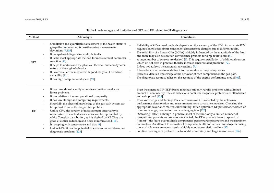
Aerospace 2019, 6, 83 21 of 53

Table 4. Advantages and limitations of GPA and KF related to GT diagnostics.

Method Advantages Limitations

GPA

- Qualitative and quantitative assessment of the health status ofgas-path component(s) is possible using measurementdeviations [9,105].

- It is capable of diagnosing multiple faults.- It is the most appropriate method for measurement parameter

selection [86].- It helps to understand the physical, thermal, and aerodynamic

nature of the engine behavior.- It is a cost-effective method with good early fault detection

capability [11].- It has high computational speed [91].

- Reliability of GPA-based methods depends on the accuracy of the ICM. An accurate ICMrequires knowledge about component characteristic changes due to different faults.

- The reliability of a Linear GPA (LGPA) is highly influenced by the magnitude of the faultand there may also be solution convergence problem for large fault values [5].

- A large number of sensors are desired [1]. This requires installation of additional sensorswhich do not exist in practice, thereby increase sensor related problems [72].

- It does not address measurement uncertainty [91].- It has a lack of access to modeling information due to proprietary issues.- It needs a detailed knowledge of the behavior of each component on the gas-path.- The diagnostic accuracy relies on the accuracy of the engine performance model [62].

KF

- It can provide sufficiently accurate estimation results forlinear problems.

- It has relatively low computational complexity.- It has low storage and computing requirements.- Since MB, the physical knowledge of the gas-path system can

be applied to solve the diagnostics problem.- Unlike GPA, the concern of measurement uncertainty is

undertaken. The actual sensor noise can be represented bywhite Gaussian distribution, as it is desired by KF. They aregood at outlier reduction and noise minimization [111].

- It is coping with sensor noise and bias [9]- Unlike GPA, it has the potential to solve an underdetermined

diagnostic problems [123].

- Even the extended KF (EKF) based methods can only handle problems with a limitedamount of nonlinearity. The estimates for a nonlinear diagnostic problems are often biasedand suboptimal [124].

- Prior knowledge and Tuning: The effectiveness of KF is affected by the unknownperformance deterioration and measurement noise covariance matrices. Choosing theappropriate covariance matrix (called tuning) for an optimized KF performance, based onprior knowledge, is a random and challenging task [125].

- “Smearing” effect: although in practice, most of the time, only a limited number ofgas-path components and sensors are affected, the KF oppositely leans to spread of(“smear”) the faults over multiple components’ performance parameters and measurementparameters. An attempt to estimate all component faults and sensor faults together usingthe available measurements results a highly nondeterministic problem [95].

- Solution convergence problem due to model uncertainty and large sensor noise [126].

Aerospace 2019, 6, 83 22 of 53

4.2. AI based Methods

The drawbacks of the MB methods forced the research community to focus on AI methods.According to Konar [127], AI is defined as “the simulation of human intelligence on a machine,in order to make the machine efficient to identify and use the right piece of “Knowledge” at a givenstep of solving a problem”. There are many different AI methods such as ANN, DL, BBN, ES, FL,and GA. The most powerful and popular types of fault diagnostic algorithms are from AI methods [12].Demonstrating and validating AI based algorithms requires operational data with appropriate quality,quantity, and type or model simulation data, in the absence of operational data. Figure 7 illustrates theconceptual framework of AI-based engine fault diagnostics. It has two parts; developing the diagnosticmechanism and its implementation. The task of developing the method includes acquisition of therequired data and preprocessing of it, training the algorithm using the processed data, and evaluatingits performance by applying the appropriate evaluation approach, for instance, using a blind test casedata as proposed by Simon [128]. The potential of AI methods on GT FDII have been widely studiedover the past several years. A comprehensive survey of these methods including their strengths andweaknesses is presented hereafter.

Aerospace 2019, 6, 83 23 of 54

4.2. AI based Methods

The drawbacks of the MB methods forced the research community to focus on AI methods.

According to Konar [127], AI is defined as “the simulation of human intelligence on a machine, in

order to make the machine efficient to identify and use the right piece of “Knowledge” at a given step

of solving a problem”. There are many different AI methods such as ANN, DL, BBN, ES, FL, and GA.

The most powerful and popular types of fault diagnostic algorithms are from AI methods [12].

Demonstrating and validating AI based algorithms requires operational data with appropriate

quality, quantity, and type or model simulation data, in the absence of operational data. Figure 7

illustrates the conceptual framework of AI-based engine fault diagnostics. It has two parts;

developing the diagnostic mechanism and its implementation. The task of developing the method

includes acquisition of the required data and preprocessing of it, training the algorithm using the

processed data, and evaluating its performance by applying the appropriate evaluation approach, for

instance, using a blind test case data as proposed by Simon [128]. The potential of AI methods on GT

FDII have been widely studied over the past several years. A comprehensive survey of these methods

including their strengths and weaknesses is presented hereafter.

Operating

Conditions

Engine Model

Component fault

Bias

Noise Data Processing Fault Diagnostics

Baseline establishment

Pattern generation

Noise filtration

Sensor validation

Detection

Isolation

Identification

Evaluation

MetricsResultsBlind Test Case

“Ground truth”

Information

Blind Test Case

Data

Results

Developing the Diagnostic Model

AI Methods

Operating

Conditions

Observed

Measurements

Data Correction

& Pattern

Generation

Operating

Conditions

Fault Diagnostic

Method

Data Validation

Suggested

Maintenance

Actions

Diagnostic Method Implementation

Figure 7. Schematics of the general AI-based GT fault diagnostic procedures. Section 1: major tasks in

developing engine diagnostics model; Section 2: the testing steps.

4.2.1. Artificial Neural Networks

An ANN is an artificial structure that processes information like a biological neuron does, except

this paradigm is mathematical instead. Its model contains sets of neurons connected to each other in

layers. Knowledge is acquired from input information (examples) through a learning process, and

Figure 7. Schematics of the general AI-based GT fault diagnostic procedures. Section 1: major tasks indeveloping engine diagnostics model; Section 2: the testing steps.

Aerospace 2019, 6, 83 23 of 53

4.2.1. Artificial Neural Networks

An ANN is an artificial structure that processes information like a biological neuron does,except this paradigm is mathematical instead. Its model contains sets of neurons connected to eachother in layers. Knowledge is acquired from input information (examples) through a learning process,and weights of connections between neurons are used to store the acquired knowledge. There arethree popular ANN learning paradigms, namely supervised, unsupervised and self-supervised [125].If the training is taken place using input and output examples it is called supervised, if it is performedusing the information derived from input data only it is called unsupervised, and if it is done utilizingthe same input and output information the learning is named self-supervised. There are various ANNalgorithms in literature such as multilayer perceptron (MLP), autoassociative neural network (AANN),radial basis function network (RBFN), probabilistic neural network (PNN), and self-organizing map(SOM). These methods have been applied to solve different engineering problems including prediction,pattern recognition/classification, and clustering [129]. They are capable of providing efficient andreliable models if a sufficient amount of data is available [90]. ANN is a powerful tool in GT modelingfor performance prediction and diagnostics due to its capability to undertake the nonlinearity of theengine behavior [130]. This is done without the need of the complex thermodynamic equations thatrelate the dependent and independent parameters.

Multilayer Perceptron

A MLP network is a feed-forward neural network consisting of input and output layers with oneor more hidden layers in between [131]. It is called feed-forward because information from the inputneurons is passed to the next layer neurons and then they compute an output based on the logisticequation and pass it to the next layer of neurons and so on until the end. The general architecture ofan MLP consists of an input layer, one or more hidden layers, and an output layer. The first layer isthe input layer that the input data goes in while the output layer, located at the end, computes theoutput value using the information coming from the hidden layers. The optimal number of hiddenlayers and neurons is determined based on a convergence criterion and the input-output mappingrelationship characteristics.

Over the past decades, several studies have been done on GT diagnostics based on an MLP [113].An ANN-based user friendly GT fault identification system was provided by Kong et al. [132].A multiple fault detection system was developed by Matuck et al. [133] using this approach which istrained on simulation data. They considered single, double, and triple component faults together withsensor noise. However, this work was limited to fault detection only. Fast et al. [90] proposed a GT faultdiagnostic schemes using MLP in order to optimize the compressor washing schedule. They have alsoindicated that ANN is a suitable approach to develop a performance prediction and fault diagnostictechniques if an operational data is available in the required quality and quantity. To answer thequestion of why neural networks are more popular than the other AI methods, Patan et al. [134]conducted a research work on two different feed-forward MLP algorithms taking into account thenonlinear behavior of the GT together with modelling uncertainty. It was pointed out that thosefault diagnostic algorithms were having better early detection ability with smaller false alarms,higher fault classification rate, and more efficient fault identification than the other AI techniques.Recently, Tayarani-Bathaie et al. [135], Mohammadi et al. [136], Kiakojoori and Khorasani [137],and Vanini et al. [62] proposed a dynamic neural network (DNN) fault diagnostic techniques for aircraftengine applications More recently, an ensemble GT fault diagnosis system was devised by Amozegarand Khorasani [138] using different types of MLP networks. Nested MLP networks were also used to afault detection and isolation application by Tahan et al. [139]. However, these methods are limited tosingle and double faults only. Moreover, they used efficiency and flow capacity deltas separately asa single component fault or in a pair as a double component fault although different studies on GTperformance degradation like [19,21], indicated that deterioration can be most significantly representedby changes of these parameters together.

Aerospace 2019, 6, 83 24 of 53

Autoassociative Neural Networks

AANNs, also known as auto-encoder, bottleneck, replicator network, or sand-glass typenetwork [140], are an important family of ANNs with three hidden layers; a mapping layer, a bottlenecklayer, and a de-mapping layer (Figure 8). They can reduce high dimensional data to a lower dimensionwith an insignificant information loss based on the concept of principal component analysis (PCA).Usually, the input and output layers contain equal numbers of neurons. The bottleneck layer is themiddle layer with the smallest number of neurons, where the important features of the input dataare captured. The number of hidden neurons associated with each hidden layer depends on theproblem type and system complexity. In this regard, more detailed information is available in [141].Compression and decompression are the two sub-networks of the general AANN structure, where theformer used to compress a high dimensional input data to a low-dimensional feature and the lattertries to reconstruct the original data from the compressed version with minimum information loss.

Aerospace 2019, 6, 83 25 of 54

analysis (PCA). Usually, the input and output layers contain equal numbers of neurons. The

bottleneck layer is the middle layer with the smallest number of neurons, where the important

features of the input data are captured. The number of hidden neurons associated with each hidden

layer depends on the problem type and system complexity. In this regard, more detailed information

is available in [141]. Compression and decompression are the two sub-networks of the general AANN

structure, where the former used to compress a high dimensional input data to a low-dimensional

feature and the latter tries to reconstruct the original data from the compressed version with

minimum information loss.

Figure 8. General architecture of autoassociative neural networks (AANN).

AANNs are widely used and very suitable for sensor data validation applications. Kramer [142]

introduced an AANN based technique for sensor validation that is capable of coping with the

nonlinearity of the data. He used the network residuals to detect and estimate sensor faults. An

AANN based sensor validation technique for a turbofan engine was proposed by Guo et al. [143]. Lu

et al. [144,145], evaluated the performance of AANNs for sensor noise reduction and bias detection

and correction. While training the noise filtering networks, they used noisy data as an input and

noise-free data as an output. The networks, therefore, tried to provide an output as close to the

desired noise-free data as possible. Besides, the effect of the number of measurements on the accuracy

of the proposed methods was tested using 4 and 9 parameters and achieved almost similar success

rates. AANNs are better at outlier removal and noise reduction than the conventional filtering

techniques [111]. A multiple sensor fault detection and isolation method using a bank of AANNs

together with a MLP based fault identification technique was developed by Zedda and Singh [118]

for a low-bypass-ratio turbofan engine purpose. It has been shown that AANNs are capable of

successful sensor failure diagnosis, even in the presence of component faults. The effectiveness of

using multiple hierarchical AANNs to diagnose single and double sensor faults in a 2-shaft industrial

GT engine was analyzed by Ogaji et al. [74]. They used three networks: the first one to separate faulty

and fault-free measurements, the second to differentiate sensor and component faults and the last to

estimate and accommodate the amount of sensor faults. This kind of diagnostic task division is

Figure 8. General architecture of autoassociative neural networks (AANN).

AANNs are widely used and very suitable for sensor data validation applications. Kramer [142]introduced an AANN based technique for sensor validation that is capable of coping with thenonlinearity of the data. He used the network residuals to detect and estimate sensor faults.An AANN based sensor validation technique for a turbofan engine was proposed by Guo et al. [143].Lu et al. [144,145], evaluated the performance of AANNs for sensor noise reduction and bias detectionand correction. While training the noise filtering networks, they used noisy data as an input andnoise-free data as an output. The networks, therefore, tried to provide an output as close to the desirednoise-free data as possible. Besides, the effect of the number of measurements on the accuracy ofthe proposed methods was tested using 4 and 9 parameters and achieved almost similar successrates. AANNs are better at outlier removal and noise reduction than the conventional filteringtechniques [111]. A multiple sensor fault detection and isolation method using a bank of AANNstogether with a MLP based fault identification technique was developed by Zedda and Singh [118] for

Aerospace 2019, 6, 83 25 of 53

a low-bypass-ratio turbofan engine purpose. It has been shown that AANNs are capable of successfulsensor failure diagnosis, even in the presence of component faults. The effectiveness of using multiplehierarchical AANNs to diagnose single and double sensor faults in a 2-shaft industrial GT engine wasanalyzed by Ogaji et al. [74]. They used three networks: the first one to separate faulty and fault-freemeasurements, the second to differentiate sensor and component faults and the last to estimate andaccommodate the amount of sensor faults. This kind of diagnostic task division is important toshare diagnostic tasks, which may improve the accuracy significantly. A combined discrete wavelettransform and AANN based diagnostic system was also developed by Tamiru et al. [146] for oilsystem, vibration system, control system diagnostics purpose. Recently, an AANN was used forsingle and double sensor and component fault diagnosis by Vanini et al. [75]. However, the sensorvalidation performance of AANN based techniques is influenced by the amount of the noise-level andthe threshold characteristics. Minimizing the number of false alarms and missed detections is equallyimportant, but they have opposite correlation (i.e., decreasing the number of false alarms by increasingthe threshold level may oppositely increase the rate of missed detections) [111].

Probabilistic Neural Network

Probabilistic neural network (PNN) is a statistical pattern classification multilayer feed-forwardnetwork based on the Bayes pattern classification strategy (based on radial basis functions (RBFs)) [147].The architecture of a typical PNN, as shown in Figure 9, consists of three layers; an input layer, a patternlayer and an output/summation layer. The input layer passes the input patterns to be classified toeach of the nodes in the pattern layer. This layer contains individual neurons corresponding to eachpattern/example in the training data set. The neurons in the pattern layer compute their responsesbased on Equation (23) and feed into the output layer neurons (Equation (24)). The output neuronsstand for the desired output groups that the network is expected to classify the input patterns into.Thus, all the connection weights between output layer and pattern layer have a value of 1. PNN canbe characterized as: they are simple in design, have a similar training nature with backpropagationalgorithm, have quite a significant pattern layer, and low computational speed [124].

Aerospace 2019, 6, 83 26 of 54

important to share diagnostic tasks, which may improve the accuracy significantly. A combined

discrete wavelet transform and AANN based diagnostic system was also developed by Tamiru et al.

[146] for oil system, vibration system, control system diagnostics purpose. Recently, an AANN was

used for single and double sensor and component fault diagnosis by Vanini et al. [75]. However, the

sensor validation performance of AANN based techniques is influenced by the amount of the noise-

level and the threshold characteristics. Minimizing the number of false alarms and missed detections

is equally important, but they have opposite correlation (i.e., decreasing the number of false alarms

by increasing the threshold level may oppositely increase the rate of missed detections) [111].

Probabilistic Neural Network

Probabilistic neural network (PNN) is a statistical pattern classification multilayer feed-forward

network based on the Bayes pattern classification strategy (based on radial basis functions (RBFs))

[147]. The architecture of a typical PNN, as shown in Figure 9, consists of three layers; an input layer,

a pattern layer and an output/summation layer. The input layer passes the input patterns to be

classified to each of the nodes in the pattern layer. This layer contains individual neurons

corresponding to each pattern/example in the training data set. The neurons in the pattern layer

compute their responses based on Equation (23) and feed into the output layer neurons (Equation

(24)). The output neurons stand for the desired output groups that the network is expected to classify

the input patterns into. Thus, all the connection weights between output layer and pattern layer have

a value of 1. PNN can be characterized as: they are simple in design, have a similar training nature

with backpropagation algorithm, have quite a significant pattern layer, and low computational speed

[124].

Figure 9. Probabilistic neural network (PNN) general architecture.

If Xij ϵ RMN (i = 1, 2, … M and j = 1, 2, … N) is the input vector with N number of input parameters

and M cases and K is the number of target classes, for an input pattern x and assuming Gaussian

probability density function (PDF), the pattern layer and output layer neurons’ outputs can be

computed, respectively, as [148]:

Figure 9. Probabilistic neural network (PNN) general architecture.

Aerospace 2019, 6, 83 26 of 53

If Xij ε RMN (i = 1, 2, . . . M and j = 1, 2, . . . N) is the input vector with N number of inputparameters and M cases and K is the number of target classes, for an input pattern x and assumingGaussian probability density function (PDF), the pattern layer and output layer neurons’ outputs canbe computed, respectively, as [148]:

Ψi j(x) =1

(2π)M2β M

exp

−(x− xi j

)T(x− xi j

)2β2

(23)

fi(x) =1

(2π)M2 βM

1Ni

N∑j=1

exp

−(x− xi j

)T(x− xi j

)2β2

(24)

where β is the smoothing parameter.The capability of PNN for GT fault diagnostics was checked for the first time by Eustace

and Merrigton [149] by implementing it to a GE low-bypass F404 military engine. Romessis andMathioudakis [150] also used this method for sensor fault diagnosis in a deteriorated enginecondition. In another study, PNNs were used for sensor fault diagnostics in a jet engine for on-boardapplication [151]. Like the other ANNs, PNN applies the concept of pattern recognition technique forfault isolation and identification tasks [152]. It uses a probabilistic measure to decide the type andlocation of the fault and to assess its magnitude. Nested PNNs have been used by Ogaji et al. [83]for sensor and component fault diagnostics in a 2-shaft aircraft engine. For this purpose, five PNNnets are used: the first is to separate the fault and no-fault patterns; the second is dedicated tosensor and component fault classification. The remaining three nets are used for component faultclassification. Then, sets of radial basis networks are integrated to quantify the magnitude of the faults.The results revealed that the proposed scheme was capable of diagnosing all the considered faultscenarios with sufficiently high accuracy. Recently, the fault classification performance of PNN wascompared with MLP and RBF by Loboda and Robles [153], and obtained similar accuracies. In general,as per this review, most of the previous PNN based GT diagnostic techniques were utilized for faultclassification tasks.

Radial Basis Function Networks

Radial basis function networks (RBF), also called a kernel function, is a multivariate approximationfunction whose value depends only on the distance from the origin or center c, i.e., the Euclideandistance [152]. It performs a nonlinear transformation over the input vector before it is fed forclassification. By using such a nonlinear function, it is possible to convert a linearly non-separableproblem to a linearly separable one. RBF increases the dimensionality of the feature vector. The mostcommonly used types of RBFs include Gaussian, multiquadric, and inverse multiquadric [154].

As shown in Figure 10, the general structure of an RBFN composed of three layers: an input layer,a hidden layer, and an output layer [131]. Like other ANNs, the number of nodes of the input layer isequal to the dimension of the input vector. The task of the hidden layer neurons is to project the inputvector into a higher dimensional vector. Hence, the number of neurons in the hidden layer must begreater than the input layer. This is because if the feature vectors are linearly non-separable in theinput dimensional space, then it is more likely that those feature vectors will be linearly separablewhen we cast them into a higher dimensional space. Once the feature vectors are linearly separable inthe M-dimensional space of the hidden layer, the linear combination of the outputs of the hidden layeris likely to give the class it belongs to. The class combination is decided by the connection weightsfrom the hidden layer nodes to the output layer nodes. In general, in this process, there are twoimportant tasks: determining the receptor and the distribution of the function and the connectionweights. Every neuron in the hidden layer represents an RBF. Due to its useful analytic properties,in addition to localization, the Gaussian function is more commonly used [154]. The number of nodes

Aerospace 2019, 6, 83 27 of 53

at the output layer is the same as the number of desired classes. Like the other MLP nets, RBF outputunits use linear summation functions.Aerospace 2019, 6, 83 28 of 54

Figure 10. General structure of radial basis function (RBF) networks.

Although RBF networks can perform different tasks like function approximation, pattern

classification, and dynamic system modelling, they have been widely used in function approximation

[125]. RBFs are capable of approximating any arbitrary function of the network layers utilizing the

training input dataset. The use of RBFs involves many advantages over backpropagation based

feedforward neural networks, for example, rapid training, very low computational expense, and very

good at interpolation, generality and simplicity [125]. They are highly localized and need a huge

quantity of training data, thereby creating a large amount of nodes that allows for rapid training. In

addition, they work better than any other training technique and are able to approximate any

continuous function [155]. However, after training, their computational speed to perform

classification or approximation is low.

The Euclidean distance is computed from the point being evaluated to the center of each neuron,

and an RBF is applied to the distance to compute the weight for each neuron [152]. The further a

neuron is from the point being evaluating the less influence it has. Leonard et al. [156] suggested a K-

means clustering technique to determine cluster centers, a K-nearest heuristic technique to determine

the width of the RBF and multiple linear regressions to determine connection weights of the layers.

Assume a set of training feature vectors and suppose C number of classes are required, for

Gaussian function the network output can be computed as [157]:

2

2

0 2exp

j

jM

j

kjk

XwXy

(25)

where yk is the kth output, wkj is the weight of the connection between the jth hidden unit and the kth

output unit, µ is the receptor/center of the function, σ (as shown in Equation (26)) is the standard

deviation of the function that decides what the spread of every RBF looks like, X is an M-dimensional

input vector, and jX is the Euclidean norm.

p

j

r

n

njniip

1 1

21 (26)

where p is the nearest number of RBF classes, r is the number of entries, µki and µkj represents the

receptors of the ith and jth hidden units of the nth entries.

Figure 10. General structure of radial basis function (RBF) networks.

Although RBF networks can perform different tasks like function approximation,pattern classification, and dynamic system modelling, they have been widely used in functionapproximation [125]. RBFs are capable of approximating any arbitrary function of the network layersutilizing the training input dataset. The use of RBFs involves many advantages over backpropagationbased feedforward neural networks, for example, rapid training, very low computational expense,and very good at interpolation, generality and simplicity [125]. They are highly localized and need ahuge quantity of training data, thereby creating a large amount of nodes that allows for rapid training.In addition, they work better than any other training technique and are able to approximate anycontinuous function [155]. However, after training, their computational speed to perform classificationor approximation is low.

The Euclidean distance is computed from the point being evaluated to the center of each neuron,and an RBF is applied to the distance to compute the weight for each neuron [152]. The further aneuron is from the point being evaluating the less influence it has. Leonard et al. [156] suggested aK-means clustering technique to determine cluster centers, a K-nearest heuristic technique to determinethe width of the RBF and multiple linear regressions to determine connection weights of the layers.

Assume a set of training feature vectors and suppose C number of classes are required, for Gaussianfunction the network output can be computed as [157]:

yk(X) =M∑

j=0

wkj exp

−‖X − µ j‖2

2σ2j

(25)

where yk is the kth output, wkj is the weight of the connection between the jth hidden unit and thekth output unit, µ is the receptor/center of the function, σ (as shown in Equation (26)) is the standard

Aerospace 2019, 6, 83 28 of 53

deviation of the function that decides what the spread of every RBF looks like, X is an M-dimensionalinput vector, and ‖X − µ j‖ is the Euclidean norm.

σi =

√√√√1p

p∑j=1

r∑n=1

(µni − µnj

)2 (26)

where p is the nearest number of RBF classes, r is the number of entries, µki and µkj represents thereceptors of the ith and jth hidden units of the nth entries.

Previously, a RBFN was often used for data cleaning prior to a fault diagnosis [157]. In thisstudy, it has also been shown that their proposed RBFN based noise filtering technique reducedthe measurement noise by 75–81%. This performance is much better than the conventional linearfilters. The problem of measurement outliers and noise was undertaken by Roy et al. [158] using aRBFN. The result showed that from 59–73% of the data outliers and noises were removed, which ismuch better than the traditional filtering methods. Ogaji et al. [5] used sets of RBFNs for gas-pathcomponents fault approximation application. The proposed method comprises of three steps: faultdetection, fault isolation, and fault identification. The first two tasks were performed using sets ofPNNs. After the detection and isolation stages, RBFN based techniques were applied to estimatethe level of component faults using their corresponding fault patterns coming from the associatedisolation networks. The applicability and performance of RBFN for a GT fault identification werecompared with a MLP by Loboda et al. [159]. They concluded that the RBF network resulted in alittle more accurate results than the conventional MLP network, however, the former requires muchmore storage capacity and computational time. Recently, a similar work has been conducted usingRBFs [160]. As per [158], RBFNs work better than many other training techniques and require muchless training computational time and cost than backpropagation based algorithms.

Self-Organizing Map

A self-organizing map (SOM) is an unsupervised learning neural network algorithm thattransforms high-dimensional input data into one or two-dimensional outputs [161]. As seen inFigure 11, its structure typically consists of an input layer and a Kohonen layer connected with a set ofweights. The colored groups on the feature map indicate the neighbor nodes arranged according totheir similarity. While training, the weights are adjusted based on the input data samples, with notarget vector available, in an unsupervised manner. The detailed mathematical expression of anSOM model and its learning mechanism can be found in [162]. Previously, it was mainly utilizedfor data clustering/classification and visualization [161,163]. It has also been applied for many otherpractical applications including rotating machinery diagnostics [164–166] and industrial and medicaldiagnostics [167–169].

Due to the lack of labeled engine operational data, implementation of such unsupervised learningnetworks in the process of gas turbine fault diagnostics may yield significant benefits. Roemer [170]proposed a modular mechanism that can detect and classify developing engine faults in a Rolls-RoyceF405 gas turbine. He integrated both supervised and unsupervised (SOM) neural network learningparadigms for life, vibration and performance monitoring purposes of the target engine. A SOM-basedclustering technique was devised by Kim et al. [171] that was used to diagnose three different faults(combustor liner burn through, bleed band leakage, and EGT sensor failures) in a mid-sized jetpropulsion engine utilizing measurement residuals from three sensors (core speed, exhaust gastemperature, and fuel flow). Come et al. [172] applied SOM for aircraft engines data visualization incombination with two other modules, one to normalize the effect of ambient condition variations on themeasurements (based on a linear regression approach) and the other for fault detection (based on thejoint use of a recursive least squares (RLS) and GLR algorithms). In another study, Cottrell et al. [173]used SOM to visualize an aircraft engine health evolution based on preprocessed data through aGeneral Linear Model (GLM). A fault diagnostic algorithm for gas turbine fuel systems was also

Aerospace 2019, 6, 83 29 of 53

introduced by Cao et al. [162] based on an improved SOM approach. In this analysis, eight differentfault cases were taken into account, which may cause the failure of three components: oil gauge,needle valve, and delivery valve. The performance of a hierarchical clustering (HC) and SOM basedfault detection and diagnosis method has been evaluated by Zhang et al. [64] using measurementdeviations obtained from a group of 19 and 16 sensors of a single shaft industrial gas turbine.As demonstration case, fault scenarios, sensor faults, bearing tilt pad wear, and early-stage pre-chamberburnout were considered. It has been stated that their developed tools are being used as part of apractically incorporated engine health monitoring systems for industrial gas turbine engines operatingacross the globe.

Aerospace 2019, 6, 83 29 of 54

Previously, a RBFN was often used for data cleaning prior to a fault diagnosis [157]. In this study,

it has also been shown that their proposed RBFN based noise filtering technique reduced the

measurement noise by 75–81%. This performance is much better than the conventional linear filters.

The problem of measurement outliers and noise was undertaken by Roy et al. [158] using a RBFN.

The result showed that from 59–73% of the data outliers and noises were removed, which is much

better than the traditional filtering methods. Ogaji et al. [5] used sets of RBFNs for gas-path

components fault approximation application. The proposed method comprises of three steps: fault

detection, fault isolation, and fault identification. The first two tasks were performed using sets of

PNNs. After the detection and isolation stages, RBFN based techniques were applied to estimate the

level of component faults using their corresponding fault patterns coming from the associated

isolation networks. The applicability and performance of RBFN for a GT fault identification were

compared with a MLP by Loboda et al. [159]. They concluded that the RBF network resulted in a little

more accurate results than the conventional MLP network, however, the former requires much more

storage capacity and computational time. Recently, a similar work has been conducted using RBFs

[160]. As per [158], RBFNs work better than many other training techniques and require much less

training computational time and cost than backpropagation based algorithms.

Self-Organizing Map

A self-organizing map (SOM) is an unsupervised learning neural network algorithm that

transforms high-dimensional input data into one or two-dimensional outputs [161]. As seen in Figure

11, its structure typically consists of an input layer and a Kohonen layer connected with a set of

weights. The colored groups on the feature map indicate the neighbor nodes arranged according to

their similarity. While training, the weights are adjusted based on the input data samples, with no

target vector available, in an unsupervised manner. The detailed mathematical expression of an SOM

model and its learning mechanism can be found in [162]. Previously, it was mainly utilized for data

clustering/classification and visualization [161,163]. It has also been applied for many other practical

applications including rotating machinery diagnostics [164–166] and industrial and medical

diagnostics [167–169].

x1 x2 xj xn. . . . . .

wij

Feature Map

Weight Matrix

Input Vector

Figure 11. Self-organizing map (SOM) architecture.

Due to the lack of labeled engine operational data, implementation of such unsupervised

learning networks in the process of gas turbine fault diagnostics may yield significant benefits.

Figure 11. Self-organizing map (SOM) architecture.

4.2.2. Deep Learning

Deep learning (DL) is a sub-field of machine learning (ML) that is used to learn feature hierarchiesof data through many layers of non-linear information processing [174]. The learning can be supervised,unsupervised or hybrid [174]. In the past few years, DL has attracted remarkable research attention withproven computational performance in several application domains including signal and informationprocessing [175], big data analysis [176], speech recognition [177], medical image analysis [178],biomedicine [179], system health management [180] and others [181].

Despite its success in the other domains, few studies have been published on the application ofDL for gas turbine fault diagnostics. A combined autoencoder and Gaussian distribution based enginegas-path anomaly detection algorithm was proposed by Luo and Zhong [182] for civil aircraft engineapplications. The autoencoder is used to denoise data uncertainties and extract the important featuresfor the Gaussian distribution-based anomaly detection module. In this assessment, measurementdeviations from 15 sensors are used in order to detect anomalies from the target engine gas pathcomponents, although no information is given about the fault scenarios considered. Yan and Yu [183]introduced a DL-based anomaly detection technique for a heavy-duty industrial gas turbine combustor.In their proposed method, stacked denoising autoencoder (SDAE) [184] is used as a data processor toavoid measurement noise and extract features for the combustor fault classification. Then extremelearning machine (ELM) neural network-based classifier is developed based on the features learned fromthe SDAE module. Recently, Xuyun et al. [185] used multiple convolutional denoising autoencoders to

Aerospace 2019, 6, 83 30 of 53

develop a fault detection technique for aircraft engines. The reported results in the above-discussedstudies encourage more utilization of DL techniques for gas turbine fault diagnostics than theconventional approaches.

4.2.3. Bayesian Belief Network

A Bayesian Belief Network (BBN) is a graphical representation of a probability distribution AIbased method that represents the cause and effect relationships among predisposing factors, faults andsymptoms [125]. The graph consists of nodes which represent a set of random variables and directededges indicating their dependencies. The degree of relationship between the variables is expressedin terms of conditional probability. In Figure 12, an example of a BBN structure referred to a gasturbine fault diagnostic is presented. In this structure, the parent nodes are dedicated to the engineperformance parameters and the child nodes to the measurement parameters. The given performanceparameters and the measurement parameters of the case engine are related through sets of directedconnections along with their associated probability values. According to the BBN approach, the enginegas path diagnostic problem can be expressed mathematically as:

P(x/z) =P(z/x)P(x)

P(z)(27)

where P(x/z) is the probability of x given z, P(z/x) is the probability of z given x, x is the independentparameter (performance parameter), z is the dependent parameter (measurement parameter), P(x) is theprobability of the independent parameter x, and P(z) is the probability of the dependent parameter z.

Aerospace 2019, 6, 83 31 of 54

engine performance parameters and the child nodes to the measurement parameters. The given

performance parameters and the measurement parameters of the case engine are related through sets

of directed connections along with their associated probability values. According to the BBN

approach, the engine gas path diagnostic problem can be expressed mathematically as:

zP

xPxzPzxP

// (27)

where P(x/z) is the probability of x given z, P(z/x) is the probability of z given x, x is the independent

parameter (performance parameter), z is the dependent parameter (measurement parameter), P(x) is

the probability of the independent parameter x, and P(z) is the probability of the dependent

parameter z.

1COMPONENT

2COMPONENT

1COMPONENT

2COMPONENT

COMPONENTn

COMPONENTn

1Parameter

t Measuremen

2Parameter

t Measuremen

mParameter

t Measuremen

PARENT NODES

(Independent Parameters) LINKS

CHILD NODES

(Dependant Parameters)

Figure 12. Typical Bayesian Belief Network (BBN) layout for engine fault identification, adapted from

Kadamb (adapted from [186].

The application of BBN for gas turbine diagnostics was started in the early 1990s by Breese et al.

[187]. Their proposed technique relies on a model-based method that integrates a BBN with an expert

system. It was implemented to assess failures on the engine oil cooling system, bearing, and bearing

temperature sensors. A few years later, Palmer [188] developed a BBN based fault diagnostic system

for the CF6 engine application, although model details were not provided. A more detailed BBN

based aircraft engine gas path fault diagnostic procedure was provided later by Kadamb [186],

Romessis et al. [189], Mathioudakis et al. [190], and Romessis and Mathioudakis [191] with the aid of

an engine performance model. They also showed the capability of their proposed method dealing

with engine diagnostic problems with measurements less than the performance parameters to be

assessed. Lee et al. [192] suggested hierarchically arranged multiple BBN models based on an offline

fault diagnosis method for industrial gas turbine engines under steady-state operating conditions. It

has been reported that the proposed method is capable of carrying out both qualitative and

quantitative diagnostics under measurement’s uncertainty.

Figure 12. Typical Bayesian Belief Network (BBN) layout for engine fault identification, adapted fromKadamb (adapted from [186].

Aerospace 2019, 6, 83 31 of 53

The application of BBN for gas turbine diagnostics was started in the early 1990s by Breese et al. [187].Their proposed technique relies on a model-based method that integrates a BBN with an expert system.It was implemented to assess failures on the engine oil cooling system, bearing, and bearing temperaturesensors. A few years later, Palmer [188] developed a BBN based fault diagnostic system for the CF6engine application, although model details were not provided. A more detailed BBN based aircraftengine gas path fault diagnostic procedure was provided later by Kadamb [186], Romessis et al. [189],Mathioudakis et al. [190], and Romessis and Mathioudakis [191] with the aid of an engine performancemodel. They also showed the capability of their proposed method dealing with engine diagnosticproblems with measurements less than the performance parameters to be assessed. Lee et al. [192]suggested hierarchically arranged multiple BBN models based on an offline fault diagnosis methodfor industrial gas turbine engines under steady-state operating conditions. It has been reported thatthe proposed method is capable of carrying out both qualitative and quantitative diagnostics undermeasurement’s uncertainty.

In the presence of large data samples, BBN can be trained in a supervised or unsupervised learningmanner, although the majority of the past attempts focused on the supervised one [193]. However,developing a BNN classifier based on expert knowledge is highly complex and time consuming, and itis subject to errors as it requires a classified training data sample based on the expert’s prior knowledgethat can be used to model the BBN structure and generate its conditional probability table (CPT).In many gas turbine applications, it is difficult to obtain the required large data samples with thefault class information. For isolation of engine fault classes with a data that has no labels assigned to,the unsupervised learning-based BBN might thus be preferable. Different algorithms exist for thispurpose such as the score-based, constraint-based, and a hybrid of these two [194].

4.2.4. Expert Systems

Expert systems (ESs) are software programs which are used to capture human expert knowledgein the form of facts and rules to solve problems or give advice as a human expert [91]. The architectureof ESs (Figure 13) comprises of four basic elements: user interface (used to acquire information anddisplay results), inference engine (deals with all the reasoning operations of the system based on knownfacts and rules), knowledge base (contains facts and rules about the problem to offer the appropriatedecision) and developer (stores information about current education) [93].

Aerospace 2019, 6, 83 32 of 54

In the presence of large data samples, BBN can be trained in a supervised or unsupervised

learning manner, although the majority of the past attempts focused on the supervised one [193].

However, developing a BNN classifier based on expert knowledge is highly complex and time

consuming, and it is subject to errors as it requires a classified training data sample based on the

expert’s prior knowledge that can be used to model the BBN structure and generate its conditional

probability table (CPT). In many gas turbine applications, it is difficult to obtain the required large

data samples with the fault class information. For isolation of engine fault classes with a data that has

no labels assigned to, the unsupervised learning-based BBN might thus be preferable. Different

algorithms exist for this purpose such as the score-based, constraint-based, and a hybrid of these two

[194].

4.2.4. Expert Systems

Expert systems (ESs) are software programs which are used to capture human expert knowledge

in the form of facts and rules to solve problems or give advice as a human expert [91]. The architecture

of ESs (Figure 13) comprises of four basic elements: user interface (used to acquire information and

display results), inference engine (deals with all the reasoning operations of the system based on

known facts and rules), knowledge base (contains facts and rules about the problem to offer the

appropriate decision) and developer (stores information about current education) [93].

User Developer

Knowledge Base

IF-THEN RULESInference

Engine

Expert System Shell

Figure 13. Configuration of an expert system (adapted from [93]).

The knowledge from the expert is first prepared in the form of a knowledgebase by a knowledge

engineer or programmer. The knowledge base contains data and facts in that specific area of

application or knowledge domain. The information in the knowledgebase is intended to replace the

human expert. The user interface presents questions to users, accepts information from them and

then provides answers and sometimes the reasoning for those answers too. The interface engine has

the job of matching the user’s input from the user interface with the data contained in the

knowledgebase to find appropriate answers. This is done using interface rules, which describe how

different items from data relate to each other and sometimes using probabilistic rules. ESs are

programmed with a series of logical rules to find a solution. Very basic ESs use Boolean logic or

decision trees. Boolean logic has two possible values, true and false, yes or no, etc. The problem is

that Boolean logic has only two values, making it difficult to represent real life problems. To avoid

the problem of decision trees, ESs typically use inference rules and chaining to reach conclusion.

Inference rules are written as IF-THEN statements which describe rules for a knowledge domain.

Numerous studies have been done using ESs in previous years, and many different ES based GT

diagnostic techniques are available in the open literature [91,195,196]. They can be broadly

categorized into rule-based, MB, and case-based techniques [91]. The earlier forms of ESs-based GT

gas-path diagnostics applied pattern recognition/matching techniques by comparing patterns of

measurement deltas with performance parameter deltas/fault signatures obtained from original

equipment manufacturers (OEM) [9]. As listed in [91], enormous ES based tools specific to different

GT models and configurations were introduced by GT manufacturers and researchers such as

TEXMAS (Turbine Engine EXpert Maintenance Advisor System), HELIX (HELicopter Integrated

eXpert), XMAN (A Tool for Automated Jet Engine Diagnostics), TIGER (Testability Insertion

Figure 13. Configuration of an expert system (adapted from [93]).

The knowledge from the expert is first prepared in the form of a knowledgebase by a knowledgeengineer or programmer. The knowledge base contains data and facts in that specific area of applicationor knowledge domain. The information in the knowledgebase is intended to replace the human expert.The user interface presents questions to users, accepts information from them and then providesanswers and sometimes the reasoning for those answers too. The interface engine has the job ofmatching the user’s input from the user interface with the data contained in the knowledgebase tofind appropriate answers. This is done using interface rules, which describe how different items fromdata relate to each other and sometimes using probabilistic rules. ESs are programmed with a series of

Aerospace 2019, 6, 83 32 of 53

logical rules to find a solution. Very basic ESs use Boolean logic or decision trees. Boolean logic has twopossible values, true and false, yes or no, etc. The problem is that Boolean logic has only two values,making it difficult to represent real life problems. To avoid the problem of decision trees, ESs typicallyuse inference rules and chaining to reach conclusion. Inference rules are written as IF-THEN statementswhich describe rules for a knowledge domain.

Numerous studies have been done using ESs in previous years, and many different ES basedGT diagnostic techniques are available in the open literature [91,195,196]. They can be broadlycategorized into rule-based, MB, and case-based techniques [91]. The earlier forms of ESs-basedGT gas-path diagnostics applied pattern recognition/matching techniques by comparing patternsof measurement deltas with performance parameter deltas/fault signatures obtained from originalequipment manufacturers (OEM) [9]. As listed in [91], enormous ES based tools specific to differentGT models and configurations were introduced by GT manufacturers and researchers such asTEXMAS (Turbine Engine EXpert Maintenance Advisor System), HELIX (HELicopter IntegratedeXpert), XMAN (A Tool for Automated Jet Engine Diagnostics), TIGER (Testability Insertion GuidanceExpert System), IFDIS (Interactive Fault Diagnosis and Isolation System), and SHERLOCK. However,knowledge from domain specific experts is usually inexact and reasoning on knowledge is oftenimprecise. An ES dealing with uncertainty and proved to be very efficient in fault diagnosis is BayesianBelief Network (BBN). However, these systems require precise inputs and rely entirely on knowledgeof experts and extensive database of rules.

4.2.5. Fuzzy Logic Methods

Fuzzy logic (FL) is a nonlinear mapping of an input feature vector into a scalar output [197]. It isone of the most widely used AI methods to approximate the relationship between dependent andindependent parameters based on a set of IF-THEN statements. The general FL approach consists offour basic components: Fuzzy Rules (sets of IF-THEN statements), Fuzzifier (the mechanism whichmaps numbers of input signals into the fuzzy set), Inference Engine (the technique used to determinethe ways in which the fuzzy sets are combined with each other) and Defuzzifier (the mechanism usedto calculate the output values) [93]. The schematic representation of a rule-based FL system is shownin Figure 14. For gas turbine diagnostics, sets of measurement parameter deltas are used as an input tothe FL system in order to compute the performance parameter deltas.

Aerospace 2019, 6, 83 33 of 54

Guidance Expert System), IFDIS (Interactive Fault Diagnosis and Isolation System), and SHERLOCK.

However, knowledge from domain specific experts is usually inexact and reasoning on knowledge

is often imprecise. An ES dealing with uncertainty and proved to be very efficient in fault diagnosis

is Bayesian Belief Network (BBN). However, these systems require precise inputs and rely entirely

on knowledge of experts and extensive database of rules.

4.2.5. Fuzzy Logic Methods

Fuzzy logic (FL) is a nonlinear mapping of an input feature vector into a scalar output [197]. It

is one of the most widely used AI methods to approximate the relationship between dependent and

independent parameters based on a set of IF-THEN statements. The general FL approach consists of

four basic components: Fuzzy Rules (sets of IF-THEN statements), Fuzzifier (the mechanism which

maps numbers of input signals into the fuzzy set), Inference Engine (the technique used to determine

the ways in which the fuzzy sets are combined with each other) and Defuzzifier (the mechanism used

to calculate the output values) [93]. The schematic representation of a rule-based FL system is shown

in Figure 14. For gas turbine diagnostics, sets of measurement parameter deltas are used as an input

to the FL system in order to compute the performance parameter deltas.

FUZZY LOGIC

Inference

Process

DEFUZZIFICATION

OUTPUT

RULES

(IF/THEN)

FUZZIFICATION

INPUT

Figure 14. Framework of a rule based fuzzy system (adapted from [124]).

After the earliest use of FL by Fuster et al. [198] in 1997, several FL based gas turbine diagnostics

techniques have been devised by other researchers. Among these, Marinai [124,199] contributed a

diagnostic model for a Rolls-Royce Trent 800 engine that can isolate both single and multiple

component faults in the presence of sensor noise and bias. Simulated data for clean and faulty GT

cases were used to test the fault detection performance of the model and the results showed that the

detection based on filtered data was very accurate with negligible missed alarms and no false alarms.

However, the investigation of the method for multiple fault diagnosis was limited to dual component

faults only. Similarly, Ganguli [200], developed GT measurements’ trend shift detection mechanism

using median filters and FL. The test results revealed that the detection based on filtered data was

very accurate with negligible missed alarms and no false alarms. In order to undertake the problem

of availability of limited numbers of sensors on a real GT service, Ganguli [197] developed a FL based

single fault isolation system for a jet engine using only four commonly available sensors. The

proposed method can isolate 95% of the faults successfully. The accuracy increased with the number

of sensors and reached 100% for eight sensors. He has also stated that FLs can work with poor quality

data. In another study, Ogaji et al. [201] proposed a diagnostic system for a modern military turbofan

engine that can identify single component faults with an accuracy of 92.5%. Recently, Kyriazis et al.

[202] developed a FL based GT compressor fault diagnostic system. Its effectiveness was compared

with pattern recognition and PNN methods. The results showed that the FL method has as good

generality and effectiveness in fault diagnostics as the other two methods.

4.2.6. Genetic Algorithm

Figure 14. Framework of a rule based fuzzy system (adapted from [124]).

After the earliest use of FL by Fuster et al. [198] in 1997, several FL based gas turbine diagnosticstechniques have been devised by other researchers. Among these, Marinai [124,199] contributed adiagnostic model for a Rolls-Royce Trent 800 engine that can isolate both single and multiple componentfaults in the presence of sensor noise and bias. Simulated data for clean and faulty GT cases wereused to test the fault detection performance of the model and the results showed that the detection

Aerospace 2019, 6, 83 33 of 53

based on filtered data was very accurate with negligible missed alarms and no false alarms. However,the investigation of the method for multiple fault diagnosis was limited to dual component faultsonly. Similarly, Ganguli [200], developed GT measurements’ trend shift detection mechanism usingmedian filters and FL. The test results revealed that the detection based on filtered data was veryaccurate with negligible missed alarms and no false alarms. In order to undertake the problem ofavailability of limited numbers of sensors on a real GT service, Ganguli [197] developed a FL basedsingle fault isolation system for a jet engine using only four commonly available sensors. The proposedmethod can isolate 95% of the faults successfully. The accuracy increased with the number of sensorsand reached 100% for eight sensors. He has also stated that FLs can work with poor quality data.In another study, Ogaji et al. [201] proposed a diagnostic system for a modern military turbofan enginethat can identify single component faults with an accuracy of 92.5%. Recently, Kyriazis et al. [202]developed a FL based GT compressor fault diagnostic system. Its effectiveness was compared withpattern recognition and PNN methods. The results showed that the FL method has as good generalityand effectiveness in fault diagnostics as the other two methods.

4.2.6. Genetic Algorithm

A genetic algorithm (GA) is a method which mimics nature on the basis of Darwin’s evolutionarytheory of “survival of the fittest” [197]. It begins with the population of randomly generated structureswhere each structure encodes a solution to the task attempt and proceeds to evolve generations.In each generation, the quality of every individual within the population is assessed by its fitness,multiple individuals are selected from the current population (based on their fitness) and modified(recombined and possibly randomly mutates). Since the fitness is a function of the objective function(OF) to be optimized, the optimum solution is reached when the OF is approaching zero and the bestfitness is associated with the value of one. It is an iterative procedure, each of which consists of threeoperators; selection, crossover and mutation [203]. During each generation, the GA improves thestructures in its current population by performing selection followed by crossover followed by mutation.It is looking for best solutions rated against fitness criteria. Thus, it avoids local optima and searchesfor a global fitness. During selection, it duplicates higher fitness structures and deletes structureswith lower fitness. Crossover results in good components of good structures combining to yieldthe better structures, and then recombines elements of good chromosomes from different genomes.Mutation creates new structures that are similar to current structures with a small pre-specifiedprobability. Figure 15 shows the schematics of the cyclic process of the three GA operators.

GAs differ from the traditional optimization techniques through the following three significantpoints [204]. Firstly, since they search parallels from a population of points, they have the ability toavoid being trapped in local optimal solution. Secondly, GAs work on the chromosome which is anencoded version of potential solution parameters rather than optimizing the parameters themselves.Thirdly, GAs use fitness score which is obtained from object functions (OFs) without an artificial overengineer black-box mathematics. In the end, like the other methods, the user typically choses the beststructures of the last population as the final solution. A more detailed description of this method canbe found in [205].

GA is often applied as an effective optimization tool to obtain a set of component parametersthat produce a set of predicted dependent parameters, through a nonlinear GT model that leads topredictions that best match the measurements [91]. The solution is obtained when the OF (which isthe measure of the difference between predicted and measured values) achieves the minimum value.A simplified illustration of GA based GT fault diagnostics strategy is given in Figure 16.

Aerospace 2019, 6, 83 34 of 53

Aerospace 2019, 6, 83 34 of 54

A genetic algorithm (GA) is a method which mimics nature on the basis of Darwin’s

evolutionary theory of “survival of the fittest” [197]. It begins with the population of randomly

generated structures where each structure encodes a solution to the task attempt and proceeds to

evolve generations. In each generation, the quality of every individual within the population is

assessed by its fitness, multiple individuals are selected from the current population (based on their

fitness) and modified (recombined and possibly randomly mutates). Since the fitness is a function of

the objective function (OF) to be optimized, the optimum solution is reached when the OF is

approaching zero and the best fitness is associated with the value of one. It is an iterative procedure,

each of which consists of three operators; selection, crossover and mutation [203]. During each

generation, the GA improves the structures in its current population by performing selection

followed by crossover followed by mutation. It is looking for best solutions rated against fitness

criteria. Thus, it avoids local optima and searches for a global fitness. During selection, it duplicates

higher fitness structures and deletes structures with lower fitness. Crossover results in good

components of good structures combining to yield the better structures, and then recombines

elements of good chromosomes from different genomes. Mutation creates new structures that are

similar to current structures with a small pre-specified probability. Figure 15 shows the schematics

of the cyclic process of the three GA operators.

CrossoverMutuation

Selection

Slave

Module

Population

Diversity

Factor

Population

Statistics

GA Operator

Parameter

Figure 15. Adaptive genetic algorithm (GA) model organization (adapted from [203]).

GAs differ from the traditional optimization techniques through the following three significant

points [204]. Firstly, since they search parallels from a population of points, they have the ability to

avoid being trapped in local optimal solution. Secondly, GAs work on the chromosome which is an

encoded version of potential solution parameters rather than optimizing the parameters themselves.

Thirdly, GAs use fitness score which is obtained from object functions (OFs) without an artificial over

engineer black-box mathematics. In the end, like the other methods, the user typically choses the best

structures of the last population as the final solution. A more detailed description of this method can

be found in [205].

Figure 15. Adaptive genetic algorithm (GA) model organization (adapted from [203]).

Aerospace 2019, 6, 83 35 of 54

GA is often applied as an effective optimization tool to obtain a set of component parameters

that produce a set of predicted dependent parameters, through a nonlinear GT model that leads to

predictions that best match the measurements [91]. The solution is obtained when the OF (which is

the measure of the difference between predicted and measured values) achieves the minimum value.

A simplified illustration of GA based GT fault diagnostics strategy is given in Figure 16.

Power Setting

Parameter

Engine Simulation

Performance Model

Fault Implanted

Simulated

Measurements

GA Based

Optimizer

Real Engine

Measurements

Fault Diagnosis

Measurement

Noise

Sensor Bias

Engine

Figure 16. Schematic diagram of GA based diagnostic strategy (adapted from [203]).

According to Zedda and Singh [118] and Singh [1], when measurement noise is assumed to be

Gaussian distribution, the suitable OF to be optimized is given as:

M

j jodj

jj

wz

wxhzxJ

12

2,

(28)

Or, if the absolute deviation is considered (this is suitable when measurement error distribution

is assumed to be other than Gaussian distribution and when modeling errors are inevitably present)

Equation (29) is more suitable.

M

j jodj

jj

wz

wxhzxJ

1

,

(29)

where J is the OF, M is the number of measurements, zj is the value of the jth measurement, h is a

vector valued function, w is power setting parameters, zodj is the value of the jth measurement in the

off-design clean condition, σj is the standard deviation of the jth measurement (noise value).

The application of GAs for a GT fault diagnosis was started in 1999 by Zedda [95], and has been

investigated by several scholars since then [206]. The problem of obtaining an accurate MB GT fault

diagnosis method in the presence of a limited number of measurements, far less than the number of

performance parameters, is undertaken by Zedda and Singh [118] using GA. The performance of this

method was evaluated and tested on Rolls-Royce (RR) RB-199, RR RB-211 and ICR-WR21 engine

types. For this purpose, the performance models for each case engine were developed utilizing the

well-known GT engine performance code TURBOMATCH. Sampath et al. [203], developed a GA-

based sensor and component fault diagnostic scheme that can deal with the nonlinearity nature of

the diagnostic problem, for a double shaft GT engine application. In this work, the effects of sensor

noise and bias and the number of sensor and component faults on the accuracy of component fault

diagnosis were analyzed using simulation data from a GT performance modelling tool, called Rolls-

Royce Aerothermal Performance (RRAP). Six gas-path components (inner and outer Fans, high-

Figure 16. Schematic diagram of GA based diagnostic strategy (adapted from [203]).

Aerospace 2019, 6, 83 35 of 53

According to Zedda and Singh [118] and Singh [1], when measurement noise is assumed to beGaussian distribution, the suitable OF to be optimized is given as:

J(x) =M∑

j=1

[z j − h j(x, w)

]2[zodj(w)•σ j

]2 (28)

Or, if the absolute deviation is considered (this is suitable when measurement error distributionis assumed to be other than Gaussian distribution and when modeling errors are inevitably present)Equation (29) is more suitable.

J(x) =M∑

j=1

z j − h j(x, w)

zodj(w)•σ j(29)

where J is the OF, M is the number of measurements, zj is the value of the jth measurement, h is avector valued function, w is power setting parameters, zodj is the value of the jth measurement in theoff-design clean condition, σj is the standard deviation of the jth measurement (noise value).

The application of GAs for a GT fault diagnosis was started in 1999 by Zedda [95], and has beeninvestigated by several scholars since then [206]. The problem of obtaining an accurate MB GT faultdiagnosis method in the presence of a limited number of measurements, far less than the number ofperformance parameters, is undertaken by Zedda and Singh [118] using GA. The performance of thismethod was evaluated and tested on Rolls-Royce (RR) RB-199, RR RB-211 and ICR-WR21 engine types.For this purpose, the performance models for each case engine were developed utilizing the well-knownGT engine performance code TURBOMATCH. Sampath et al. [203], developed a GA-based sensorand component fault diagnostic scheme that can deal with the nonlinearity nature of the diagnosticproblem, for a double shaft GT engine application. In this work, the effects of sensor noise and biasand the number of sensor and component faults on the accuracy of component fault diagnosis wereanalyzed using simulation data from a GT performance modelling tool, called Rolls-Royce AerothermalPerformance (RRAP). Six gas-path components (inner and outer Fans, high-pressure compressor (HPC),high-pressure turbine (HPT), low-pressure turbine (LPT), and Nozzle), when affected individually or inpair (as a single component fault (SCF) and double component fault (DCF) cases), were analyzed using16 gas-path measurements in the presence of two and four concurrent sensor faults. For this purpose,six SCF and 15 DCF classes were considered. A GA based GT fault diagnosis method was used to findan optimal combination of a set of performance parameters and the corresponding set of best matchmeasurement parameters, through a non-linear performance simulation model [108]. A generalizedGA based GT fault classification method was proposed by Loboda et al. [207] using a thermodynamicmodel that is applicable to multiple operating point conditions for both steady state and transientcases. Li and Pilidis [103] and Li et al. [208] applied GA for a GT performance adaptation in order toassess the engine’s health status. For this purpose, the information from the measurements was usedto estimate the component faults at a specified design point and off-design operating condition.

Recently, the fault diagnosis effectiveness of an NLGPA and a GA based method was comparedby Kong et al. [209], applied on a 2-spool turbofan engine. They showed that the diagnostic MB on GAis better than the NLGPA, particularly when sensor noise and bias are considered. In a similar manner,Kong [93] investigated the diagnostic effectiveness of GA in comparison with NLGPA and fuzzy-neurotechniques taking in to account measurement uncertainty and sensor fault effects. The test resultsindicated that the GA based method showed a reliable accuracy than the NLGPA, especially in thepresence of sensor noise and bias.

Aerospace 2019, 6, 83 36 of 53

4.2.7. Hybrid AI Methods

In spite of the fact that it is impossible to find a single-technique which can undertake all theconcerns of diagnostics, it would be fascinating to combine two or more methods in an attempt tooffset the limitations of one with the advantages of another [1]. With regard to this, many combined AItechniques are proposed by different authors including Genetic-neural network, Genetic-fuzzy logic,fuzzy–neural networks (FNNs), and neural–fuzzy systems [210,211]. Green and Allen [212] discussedthe benefits of combining ANN with other AI methods for diagnostics and prognostics. GA is appliedas an effective optimization tool to obtain a set of component parameters that produce a set of predicteddependent parameters, through a non-linear GT model that leads to predictions which best match themeasurements [91]. In FL-based techniques, the optimal selection of fuzzy sets with the appropriatemembership functions (MFs) is essential. However, in the conventional FL applications, there is nodefined function to determine the number of fuzzy sets and MFs [111]. It is indicated in here that GAsare capable of selecting the optimal number of fuzzy sets and MFs automatically, thereby enhancingthe performance of the FL. Kobayashi and Simon [213] investigated the effectiveness of a MB hybridneural network GA technique for a turbofan engine application. The neural network scheme wasutilized to diagnose GT component faults while the GA scheme is used for sensor fault evaluation.The sensor and component fault diagnostic potential of a hybrid ANN and GA based model wasalso developed and implemented on advanced cycle Intercooled Recuperated (ICR) WR21 engineby Sampath and Singh [211]. In this model, the task of the ANN module was to pre-process andvalidate the GT data, whereas the GA module was to isolate and identify faults. It has been shownthat the accuracy, reliability, and consistency of the results obtained from the hybrid technique arebetter than ANN and GA based algorithms. A RBFN was applied for a GT fault identification purpose,integrated with a MB KF fault diagnosis scheme by Simani and Fantuzzi [155]. In this algorithm,the KF based scheme was accountable to detect and isolate the faults using measurement residual,while the RBFN quantified the magnitude of the faults based on pattern recognition approach.

4.2.8. Advantages and Limitation of AI Methods

Table 5 presents a summary of the advantages and limitations of AI-based methods reviewedabove. This may help beginners of this field in selecting the appropriate diagnostic approach forvariety of engine diagnostic problems. In general, unlike MB methods, AI-based methods can handlethe effect of sensor noise and bias, the possible existence of multiple faults simultaneously, the faultidentification problem using a limited number of instrumentation suite, and the nonlinear relationshipbetween the measurement parameters and the performance parameters. However, most AI-basedtechniques cannot give confidence limits on the output. In addition, they are not capable of diagnosingfaults outside the domain of the data to which they have been exposed during training.

4.3. Strengths and Weaknesses of the Gas-Path Diagnostic Methods

Table 6 presents the summary of these methods regarding their capability of undertaking thechallenges discussed in Section 3.1 and fulfilling the desirable attributes of an effective diagnostic systemstated in Section 3.2. It gives a clear view of the pros and cons of the aforementioned diagnostic methods,and it is important to choose an appropriate diagnostics system for a particular diagnostics problem.

Aerospace 2019, 6, 83 37 of 53

Table 5. Advantages and limitations of AI-based methods regarding GT diagnostics.

Method Advantages Limitations

ANN

- They can deal with the nonlinear nature of the engine performance.- They are capable of learning with time.- They are very good in data fusion [1].- Training can be done by means of information extracted from performance data without knowing the

details of the gas-path system.- They can handle multiple fault problems [83].- They can deal with measurement uncertainty (noise and bias) [9].- They can be applied for onboard applications due to their high computational speed [11].- They are able to deal with large component faults in the presence of sensor faults [83].- They are more appropriate to handle diagnostics problems with limited numbers of measurements [1].- They are relatively easy to implement for both engine performance modeling and diagnostics [214].

- Since they are unable to perform reliably outside the range of thedata they are trained on, a huge amount of data that can sufficientlyrepresent the entire life of the engine condition is required.

- They require high computational time (during training).- If operational data is used to develop the methods, retraining will be

required during engine overhaul and/or its operating conditionchanges [5].

- Diagnostic error increases with an increase in the number ofoperating points. But this problem can be solved by correcting thedata towards ambient condition and load variations [5].

- The process in the hidden layers is not visible (they are black-boxmodels).

FL

- Like other AI methods, they are model-free, can handle diagnostic problems which are difficult to bedescribed and solved mathematically.

- Fuzzy rules are derived from the available GT data for training. This makes them particularly suited forfinding solutions to problems for which there are no exact solution, but only with a large number ofexamples [124].

- They are capable of generalizing from examples [124].- They can handle multiple fault problems partially [9].- They are able to deal with the non-linear nature of gas-path problems [11].- They are coping with measurement noise and sensor bias [91].- Like ANNs, FLs could perform data-fusion [2].- Like ANN, FL-based systems could be utilized for online diagnosis application due to the fast

computational capability in inference mode [11].

- Fuzzy rules depend on the knowledge of subject expert anddiagnosis accuracy depends on the available rules.

- Large quantity of rules and training data sets are required [2].- They are not as effective in quantitative fault diagnostics as ANN [5]- Like other AI systems, they are poor at recognizing new datasets that

the model does not see during training [124]. Hence, for a betteraccuracy, a massive amount of data is necessary.

- Does not admit model robustness.- Difficult to define exact queries that identify specific faults.

GA

- It is able to deal with measurement noise and bias.- It provides good results when integrated with other MB as well as DD systems [1].- Like ANN, it can deal with engine diagnostic problems with limited instrumentation suites available.- It can optimize the engine performance functions without the need to solve complex equations like the

other mathematical optimization approaches [208].- It can perform both qualitative and quantitative diagnostics [5].- It can perform simultaneous fault analysis [215].- It can deal with the non-linear nature of the engine behavior [208].

- It requires long computational time than traditional optimizationtechniques, especially as population and generation numbers grow[105].

- As the number of simultaneous faults increases, the convergencetime increases [125].

- In order to check the consistence in the GA optimization results,multiple runs are often required [5].

Aerospace 2019, 6, 83 38 of 53

Table 5. Cont.

BBN

- It is graphical, and it is easy to visualize the model variables and its diagnostic results.- It is capable of performing multiple simultaneous fault analysis [188].- It can perform data fusion [2].- It can provide better, more flexible and robust diagnostic solutions [191].- Unlike ANN, it requires a short retraining time because gas turbine model hardware changes can be easily

entered [124].- Unlike ANN, BBN can include generic faults that are not considered during the training process of the

diagnostic system [188].- After completing the BBN model utilizing a gas turbine simulation model, it does not need to run the

model gaining in computational speed [124].- It is more realistic to make diagnosis expressing the probability of whether a fault occurred or not, than

expressing a deterministic answer [10].

- High computational requirement [186].- Gathering the required information for setting a BBN model is

tedious and time consuming [125].- It requires a well-trained developer to set it up [188].- As the number of nodes and edges increase the model complexity

and computational and storage requirements increase [216].- Measurement uncertainties and operating condition variations affect

its accuracy [217].

ExpertSystem

(ES)

- It is preferable when the diagnostic problem is well understood, stable, and human experts are availableto develop the knowledgebase.

- It is relatively simple to develop and easy to understand.- It is a more suitable technique for stable and predictable GT operating conditions, if potential faults can be

defined easily.- The knowledgebase does not represent only a single human expert knowledge, rather a group as a whole.

This helps to eliminate biases from individuals [59].- It is more important for applications in remote areas that maintenance experts cannot be found in nearby

distance [59].

- The knowledge base may suffer from measurement uncertainties andincomplete or missing data. This problem could have a significanteffect on reliability and accuracy of answers provided by the system.

- Like any software program, the inference engine running missingrules or incorrect data process influences its accuracy and reliability.

- It is highly dependent on the knowledgebase, which covers only asmall amount of knowledge, and are incapable of dealing withproblems outside this domain. If experts are wrong, the output willalso be wrong. Thus, it requires up-to-date knowledge of the humanexperts along with a significant set of rules.

- The knowledge acquisition task is time consuming.- It requires high establishment cost due to luck of human experts [59].

Aerospace 2019, 6, 83 39 of 53

Table 6. Comparative summary of the major diagnostic methods concerning their capability towards the desirable attributes.

Method Category Coping with Noise & Bias[9,91]

Ability to Deal with ProblemNon-Linearity [9,91]

No. of SensorsRequired [9]

Data Fusion Ability[2,9]

ComputationalSpeed [2,91]

SFI Capability[9]

Ability to ProvideQuantitative Solutions [2]

LGPA MB No Incapable M ≥ N L H Capable Capable

NLGPA MB No Capable M ≥ N L FH Capable Capable

LKF MB Partial Incapable N < M AA H Capable Capable

NLKF MB Partial Capable N < M AA H Capable Capable

ANN DD Yes Capable N < M FH H Capable Capable

GA MB/AI Yes Capable N < M FH L Capable Capable

FL DD Yes Capable N < M H H Capable Partial

BBN DD Yes Capable N < M H L Capable Capable

ES DD Yes Capable N < M Fairly high FH Capable Capable

Method SystemComplexity [91]

MFIICapability [9,87] Explanation Facility [87] Adaptability

[87]Memory

Requirement [9,87]Online/OfflineApplication [9]

User FriendlyInterface [11] Flexibility [2]

LGPA L Capable - NF L Offline F H

NLGPA L Capable - NF L Offline F H

LKF FL Capable NF NF L Both F AA

NLKF Mm Capable NF NF L Both F AA

ANN FH Partial NF F H Both F L

GA FH Partial - F H Offline NF AA

FL H Partial - F H Both F A

BBN H Partial NF F H Offline F F

ES H Partial NF F H Offline F A

L, low; Mm, medium; AA, above average; FL, fairly low; FH, fairly high; H, high; F, favorable; NF, not favorable; N, number of performance parameters; M, number ofmeasurement parameters.

Aerospace 2019, 6, 83 40 of 53

5. GT Diagnostic Methods Validation Techniques

In the field of GT diagnostics, method validation is a critical issue. GT users need a practical toolto evaluate the performance and effectiveness of any algorithm before they decide to incorporate intotheir plants. However, there are no standardized commercial tool for this purpose. The evaluationapproaches that the research community was using until now are:

1. Performance Metrics Approach: Performance metrics can be used to measure the detection,isolation, and identification performance of a fault diagnostics algorithm [218]. The detectionmetric measures how accurately the detection algorithm detects abnormal operating conditions.The isolation metrics evaluates how successfully the isolation part of the diagnostic frameworkdistinguishes the fault types and their locations. Also, the identification metrics measureshow accurately the diagnostics system estimates the magnitude of the faults. A more detaileddescription about this concern together with sample performance metrics is available in [219].The majority of the fault diagnostic methods available in the open domain are evaluated basedon this approach. A fault diagnostics performance metric associated with the fault detection andisolation reliability of four different methods for aircraft engines is presented by Simon et al. [220].

2. Benchmark Fault Cases Approach: The generally accepted and implemented solution to obtainthe required performance data for diagnostic method development and validation is implantingfault cases corresponding to the possibly existing faults into the GT performance model [113,221].However, there exists some inconsistencies concerning the range of the performance parameterlosses that different gas-path faults are represented by [222]. The issue of using benchmark faultcases has also been thoroughly studied by the OBIDICOTE (On Board Identification, Diagnosis andControl of GT Engines) Project conducted by the European research community [223]. The projectidentified a set of benchmark fault cases, which have been used by several researchers so far toevaluate their engine fault diagnostic methods [191,211,224]. The effectiveness of using some setsof benchmark fault cases to evaluate the performance of a diagnostic system is further investigatedby the engine health management industry review (EHMIR) established under The TechnicalCooperation Program (TTCP) [224]. TTCP is a collaboration forum for defense science andtechnology (DST) between five nations, namely, UK, USA, Canada, Australia and New Zealand.The effort of this forum resulted in a reference engine problem, together with a recommendationof an evaluation environment for different diagnostics algorithms. Based on the recommendationof the aircraft engine health monitoring community, recently, NASA’s research team developeda public benchmark gas-path fault diagnostics techniques’ performance evaluation softwarereferred to as the Propulsion Diagnostic Method Evaluation Strategy (ProDiMES), applicable toaircraft engines [220]. In this software, four different methods are included; Weighted LeastSquares, PNN, Performance Analysis Tool, and Generalized Observer/Estimator. Moreover,the field GT condition monitoring and diagnostics has been studied for many years by the researchteam of the Laboratory of Thermal Turbomachines of the National Technical University of Athens(LTT/NTUA) [12] and Cranfield University (CU) [1] and proposed many different techniques.These groups showed the effectiveness of using benchmark fault cases to develop and evaluatethe performance of diagnostic algorithms.

3. Comparison of Methods Approach: As a third alternative, there are also some self-conductedcomparative evaluation (a one-to-one comparison of methods) based research works to assessthe diagnostic performance of different themes [113,221]. In this category, previously publishedpapers are used as benchmark methods to compare the performance of the newly developedalgorithm. However, this approach has limitations due to the reason that most of the available GTdiagnostic methods targeted different engine problems and degree of complexity under variety ofdiagnostic conditions (i.e., operating modes, measurement system, deterioration profile etc.) [224].

Aerospace 2019, 6, 83 41 of 53

6. Conclusions and Future Research Directions

Gas turbine (GT) gas-path fault diagnostics is a key element of an overall engine condition-basedmonitoring (CBM) system providing enhanced safety, reliability, and availability along with optimaloperation and maintenance costs. In consideration of this role, an effective and reliable gas-pathdiagnostic technique is critical. This paper was devoted to discussing various issues related togas-path diagnostics including engine physical faults, challenges and desirable attributes of agas-path diagnostics, state-of-the-art methods, and verification and validation approaches. The pastefforts on gas-path diagnostics have focused on the aspects of data filtration, sensor validation,and component fault diagnostics. Variety of methods associated with these aspects, beginning with theconventional methods to the most sophisticated artificial intelligence (AI) based ones, were reviewed.Due to their remarkable capability of handling the available challenges and meet the majority of thedesirable attributes, recent efforts paid more attention to AI methods. Particularly, artificial neuralnetworks (ANNs) have been widely used for both qualitative and quantitative diagnostic applications,although the majority of the investigations were limited to single sensor fault and/or single componentfault analysis. However, in order to avoid the barriers between system developers and engine users andget their interest to invest and incorporate gas-path diagnostic technologies into their plants, there aretwo main issues that the gas-path diagnostics research community should give attention to: improvingthe effectiveness and reliability of the available fault diagnostic systems and developing practical toolsto evaluate the effectiveness of the proposed techniques. With that in mind, the following furtherstudies should be carried out.

• The need for a standardized gas-path diagnostic problem definition. According to this survey,there is no consensus between researchers in defining and representing gas-path diagnosticproblems (terminologies, component fault representation, ranges of sensor/component faults,and the number and type of faults corresponding to different engine configurations that possiblyexist in the engines lifetime). This inconsistency may confuse young researchers of the field,create barriers in exchanging gas-path diagnostic related ideas/solutions and performing aone-to-one comparison of different algorithms.

• The review on GT performance deterioration revealed that the degradation profile correspondingto each gas-path’s faults is not consistent. This may lead to an incorrect representation ofcomponents deterioration, and thereby unreliable fault diagnostic results. Hence, there should bemore investigations in this regard.

• Most of the devised techniques for simultaneous fault analysis were restricted to qualitativesolutions (i.e., detecting and isolating without estimating the level of the fault, which is a veryimportant step in the maintenance decision). Moreover, the accuracy of the available limitedquantitative approaches requires improvement for multiple fault scenarios. Development of aneffective gas-path diagnostic system that can perform both qualitative and quantitative diagnosticsof both single and multiple fault scenarios thus needs further investigation.

• Development of efficient hybrid methods. Most of the available gas-path diagnostic methods aresingle-technique-based and it is difficult to find single-technique which can address all gas-pathdiagnostic related challenges along with providing accurate diagnostic results. It is recommendedto combine two or more methods based on their merits.

• Development of integrated platforms. Although a large number of diagnostic methods have beendevised so far, the majority of those methods considered different platforms with different levelsof complexity and applied for different engine system monitoring (such as sensor, component,vibration, controller, and fuel and oil systems). Integration of verity of methods into a diagnostictool being capable of addressing the entire GT system problems is required.

• Establishment of a practical approach to verification and validation. Engine users need practicaltools to objectively assess the effectiveness (i.e., the technical and economic feasibility) of newlyproposed solutions and determine its advantages over the existing maintenance practices before

Aerospace 2019, 6, 83 42 of 53

incorporating into their plants. However, there are no internationally accepted standards orunified frameworks that can be applied for this purpose. Hence, the establishment of practicalverification and validation approaches requires attention in this field.

• Development of user-friendly gas-path diagnostic software. Regarding engine performancesimulation, there are some powerful commercial software available. Conversely, other than thetraditional techniques, there are no advanced software tools based on AI methods. Therefore,user-friendly gas-path diagnostic software that can acquire, preprocess and validate performancedata, assess the condition of engines and suggest the appropriate maintenance actions is required.

Author Contributions: A.D.F. wrote the manuscript and A.T.B., S.I.G. and K.G.K. supervised and made somecritical revisions. All authors have read and approved the final manuscript.

Funding: This research was partially funded by the Knowledge Foundation (KKS) under the project DIAGNOSISwhile the APC was funded by Mälardalen University (MDH).

Acknowledgments: The authors would like to acknowledge Universiti Teknologi PETRONAS (UTP) andMälardalen University (MDH) for supporting this research financially as well as for all the facilities provided.

Conflicts of Interest: The authors declare no conflict of interest.

Nomenclature and Abbreviations

AANN Auto-associative neural networkAI Artificial intelligenceANN Artificial neural networkBBN Bayesian belief networkCBM Condition-based maintenanceCCPP Combined cycle power plantCPT Conditional probability tableDB Data basedDCF Double component faultDD Data drivenDL Deep learningDNN Dynamic neural networkDOD Domestic object damageDST Defense science and technologyEGT Exhaust gas temperatureEHM Engine health monitoringEHMIR Engine health management industry reviewEKF Extended Kalman filterELM Extreme learning machineES Expert systemFCM Fault coefficient matrixFDD Fault detection and diagnosticsFDI Fault detection and isolationFDIA Fault detection, isolation and accommodationFDII Fault detection, isolation and identificationFDIR Fault detection, isolation and recoveryFL Fuzzy logicFOD Foreign object damageGA Genetic algorithmGLR Generalized likelihood ratioGPA Gas-path analysisGT Gas turbineHC Hierarchical clustering

Aerospace 2019, 6, 83 43 of 53

HELIX HELicopter Integrated eXpertHPC High pressure compressorHPT High pressure turbineIATA International air transport associationICM Influence coefficient matrixIEKF Iterated extended Kalman filterIFDIS Interactive Fault Diagnosis and Isolation SystemKF Kalman filterLCC Life cycle costICR Intercooled recuperatedLGPA Linear gas-path analysisLKF Linear Kalman filterLPT Low pressure turbineMAP Maximum a posteriorMB Model basedMF Membership functionML Machine learningMLP Multiple layer perceptronMLPNN Multiple layer perceptron neural networkMRO Maintenance repair and overhaulMSE Mean square errorNBS National bureau of standardsNLGPA Nonlinear gas-path analysisNLKF Nonlinear Kalman filterNTUA National technical university AthensOBDICOTE On board identification, diagnosis and control of gas turbineOEM Original equipment manufacturerOF Object functionPCA Principal component analysisPNN Probabilistic neural networkPR Pressure ratioPWL Piecewise linearRBF Radial basis functionRBFN Radial basis function networkRMS Root mean squareRRAP Rolles-Royce aerothermal performanceSCF Single component faultSDAE Stacked denoising autoencoderSOM Self-organizing mapSTORM Self-tuning onboard real-time modelSVM State variable engine modelTCF Triple component faultTEXMAS Turbine Engine EXpert Maintenance Advisor SystemTIGER Testability Insertion Guidance Expert SystemTTCP The technical cooperation programXMAN A Tool for Automated Jet Engine DiagnosticsΓ Flow capacityη Isentropic Efficiency

References

1. Singh, R. Advances and opportunities in gas path diagnostics. In Proceedings of the 15th ISABE, Bangalore,India, 2–7 September 2003. Paper No. ISABE-2003-1008.

2. Bechini, G. Performance Diagnostics and Measurement Selection for On-Line Monitoring of Gas TurbineEngines. Ph.D. Thesis, Cranfield University, Bedford, UK, 2007.

Aerospace 2019, 6, 83 44 of 53

3. Association, I.A.T. Airline Maintenance Cost: Executive Commentary. 2011. Available online: http://www.iata.org/workgroups/Documents/MCTF/AMC_ExecComment_FY09.pdf (accessed on 10 April 2019).

4. McFadden, M.; Worrells, D.S. Global outsourcing of aircraft maintenance. J. Aviat. Technol. Eng. 2012, 1, 4.[CrossRef]

5. Ogaji, S.O.T.-O. Advanced Gas-path Fault Diagnostics for Stationary Gas Turbines. Ph.D. Thesis,Cranfield University, Bedford, UK, 2003.

6. Boyce, M.P. Gas Turbine Engineering Handbook; Elsevier: Amsterdam, The Netherlands, 2011.7. Factbook, C. The World Factbook. 2010. Available online: https://www.cia.gov/library/publications/the-

world-factbook (accessed on 15 April 2019).8. Lengyel, G.J. Department of Defense Energy Strategy: Teaching an Old Dog New Tricks; DTIC Document;

DTIC: Fort Belvoir, VA, USA, 2007.9. Marinai, L.; Probert, D.; Singh, R. Prospects for aero gas-turbine diagnostics: A review. Appl. Energy 2004, 79,

109–126. [CrossRef]10. Stamatis, A.G. Engine condition monitoring and diagnostics. In Progress in Gas Turbine Performance;

Benini, E., Ed.; InTech: Rijeka, Croatia, 2013; pp. 187–212. [CrossRef]11. Tahan, M.; Tsoutsanis, E.; Muhammad, M.; Karim, Z.A. Performance-based health monitoring, diagnostics and

prognostics for condition-based maintenance of gas turbines: A review. Appl. Energy 2017, 198, 122–144.[CrossRef]

12. Romesis, C.; Aretakis, N.; Roumeliotis, I.; Alexiou, A.; Tsalavoutas, A.; Stamatis, A.; Mathioudakis, K.Experiance with condition-based maintenance related methods and tools for gas turbines. In Proceedingsof the Future of Gas Turbine Technology, 7th International Gas Turbine Conference, Brussels, Belgium,14–15 October 2014.

13. Meher-Homji, C.B.; Chaker, M.; Motiwalla, H. Gas turbine performance deterioration. In Proceedings of the30th Turbomachinery Symposium, Houston, TX, USA, 17–20 September 2001; pp. 17–20.

14. Meher-Homji, C.B.; Matthews, T.; Pelagotti, A.; Weyermann, H. Gas Turbines and Turbocompressors for LNGservice. In Proceedings of the 36th Turbomachinery symposium, Houston, TX, USA, 11–13 September 2007.

15. Marinai, L.; Singh, R.; Curnock, B.; Probert, D. Detection and prediction of the performance deterioration ofa turbofan engine. In Proceedings of the International Gas Turbine Congress, Tokyo, Japan, 2–7 November2003; pp. 2–7.

16. Urban, L.A. Parameter selection for multiple fault diagnostics of gas turbine engines. ASME J. Eng. Power1975, 97, 225–230. [CrossRef]

17. Meher-Homji, C.B.; Chaker, M.; Bromley, A.F. The fouling of axial flow compressors: Causes, effects,susceptibility, and sensitivity. In Proceedings of the ASME Turbo Expo 2009: Power for Land, Sea, and Air,Orlando, FL, USA, 8–12 June 2009; pp. 571–590.

18. Diakunchak, I.S. Performance deterioration in industrial gas turbines. J. Eng. Gas Turbines Power 1992, 114,161–168. [CrossRef]

19. Morini, M.; Pinelli, M.; Spina, P.; Venturini, M. Influence of blade deterioration on compressor and turbineperformance. J. Eng. Gas Turbines Power 2010, 132, 032401. [CrossRef]

20. Melino, F.; Morini, M.; Peretto, A.; Pinelli, M.; Spina, P.R. Compressor fouling modeling: Relationship betweencomputational roughness and gas turbine operation time. J. Eng. Gas Turbines Power 2012, 134, 052401.[CrossRef]

21. Saravanamuttoo, H.I.H.; Lakshminarasimha, A.N. A Preliminary Assessment of Compressor Fouling;ASME: New York, NY, USA, 1985.

22. Aretakis, N.; Roumeliotis, I.; Mathioudakis, K. Performance model “zooming” for in-depth component faultdiagnosis. J. Eng. Gas Turbines Power 2011, 133, 031602. [CrossRef]

23. Lakshminarasimha, A.N.; Boyce, M.P.; Meher-Homji, C.B. Modelling and analysis of gas turbine performancedeterioration. In Proceedings of the ASME 1992 International Gas Turbine and Aeroengine Congress andExposition, Cologne, Germany, 1–4 June 1992; p. V004T010A022.

24. Meher-Homji, C.B.; Bromley, A. Gas turbine axial compressor fouling and washing. In Proceedings of the33rd Turbomachinery Symposium, Houston, TX, USA, 21–23 September 2004; pp. 20–23.

25. Zwebek, A.; Pilidis, P. Degradation effects on combined cycle power plant performance - Part I: Gas turbinecycle component degradation effects. J. Eng. Gas Turbines Power 2003, 125, 651–657. [CrossRef]

Aerospace 2019, 6, 83 45 of 53

26. Kurz, R.; Brun, K. Gas Turbine Performance—What Makes the Map. In Proceedings of the 29th Texas A&MTurbomachinery Symposium, Houston, TX, USA, 18–21 September 2000; pp. 18–21.

27. Tarabrin, A.P.; Schurovsky, V.A.; Bodrov, A.I.; Stalder, J.P. An analysis of axial compressor fouling and a bladecleaning method. J. Turbomach. 1998, 120, 256–261. [CrossRef]

28. Ogiriki, E.A.; Li, Y.G.; Nikolaidis, T.; Isaiah, T.E.; Sule, G. Effect of fouling, thermal barrier coating degradationand film cooling holes blockage on gas turbine engine creep life. Procedia CIRP 2015, 38, 228–233. [CrossRef]

29. Aker, G.F.; Saravanamuttoo, H.I.H. Predicting gas turbine performance degradation due to compressorfouling using computer simulation techniques. J. Eng. Gas Turbines Power 1989, 111, 343–350. [CrossRef]

30. Yang, H.; Xu, H. The new performance calculation method of fouled axial flow compressor. Sci. World J.2014, 2014, 906151. [CrossRef] [PubMed]

31. Tarabrin, A.; Schurovsky, V.; Bodrov, A.; Stalder, J.-P. Influence of Axial Compressor Fouling on Gas TurbineUnit Perfomance Based on Different Schemes and With Different Initial Parameters. In Proceedings ofthe ASME 1998 International Gas Turbine and Aeroengine Congress and Exhibition, Stockholm, Sweden,2–5 June 1998; p. V004T011A006.

32. Mezheritsky, A.D.; Sudarev, A.V. The Mechanism of Fouling and the Cleaning Technique in Application toFlow Parts of the Power Generation Plant Compressors. In Proceedings of the ASME 1990 International GasTurbine and Aeroengine Congress and Exposition, Brussels, Belgium, 11–14 June 1990; p. V004T011A003.

33. Seddigh, F.; Saravanamuttoo, H. A proposed method for assessing the susceptibility of axial compressorsto fouling. In Proceedings of the ASME 1990 International Gas Turbine and Aeroengine Congress andExposition, Brussels, Belgium, 11–14 June 1990; p. V003T007A012.

34. Boyce, M.P.; Gonzalez, F. A study of on-line and off-line turbine washing to optimize the operation of a gasturbine. J. Eng. Gas Turbines Power 2007, 129, 114–122. [CrossRef]

35. Stalder, J.P. Gas Turbine Compressor Washing State of the Art: Field Experiences. J. Eng. Gas Turbines Power2001, 123, 363. [CrossRef]

36. Casari, N.; Pinelli, M.; Suman, A.; di Mare, L.; Montomoli, F. An Energy-Based Fouling Model for GasTurbines: EBFOG. J. Turbomach. 2017, 139, 021002. [CrossRef]

37. Maiwada, B.; Mu’az, N.I.; Ibrahim, S.; Musa, S.M. Impacts of Compressor Fouling on the Performance of GasTurbine. Int. J. Eng. Sci. 2016, 2118–2125. [CrossRef]

38. Aretakis, N.; Roumeliotis, I.; Doumouras, G.; Mathioudakis, K. Compressor washing economic analysis andoptimization for power generation. Appl. Energy 2012, 95, 77–86. [CrossRef]

39. Diakunchak, I.S. Performance Improvement in Industrial Gas Turbines. In Proceedings of the JointASME/IEEE Power Generation Conference, Kansas City, KS, USA, 17–22 October 1993. [CrossRef]

40. Wilcox, M.; Baldwin, R.; Garcia-Hernandez, A.; Brun, K. Guideline for Gas Turbine Inlet Air Filtration Systems;Gas Machinery Research Council: Dallas, TX, USA, 2010.

41. Singh Grewal, M. Gas Turbine Engine Performance Deterioration Modelling and Analysis. Ph.D. Thesis,Cranfield University, Bedford, UK, 1988.

42. Salar, A.; Hosseini, S.M.; Zangmolk, B.R.; Sedigh, A.K. Improving model-based gas turbine fault diagnosisusing multi-operating point method. In Proceedings of the 2010 Fourth UKSim European Symposium onComputer Modeling and Simulation (EMS), Pisa, Italy, 17–19 November 2010; pp. 240–247.

43. Qingcai, Y.; Li, S.; Cao, Y.; Zhao, N. Full and Part-Load Performance Deterioration Analysis of IndustrialThree-Shaft Gas Turbine Based on Genetic Algorithm. In Proceedings of the ASME Turbo Expo 2016:Turbomachinery Technical Conference and Exposition, Harbin, China, 13–17 June 2016; p. V006T005A016.

44. Kurz, R.; Brun, K. Degradation in Gas Turbine Systems. J. Eng. Gas Turbines Power 2000, 123, 70–77. [CrossRef]45. Kurz, R.; Brun, K. Gas turbine tutorial—maintenance and operating practices effects on degradation and

life. In Proceedings of the 36th Turbomachinery Symposium, Houston, TX, USA, 11–13 September 2007;pp. 10–13.

46. Gannan, A. Cascade Testing and CFD Applied to Gas Turbine Performance Improvement with CompressorCleaning. Ph.D. Thesis, Cranfield University, Bedford, UK, 2010.

47. Wilcox, M.; Kurz, R.; Brun, K. Successful Selection and Operation of Gas Turbine Inlet Filtration Systems.In Proceedings of the 40th Turbomachinery Symposium, Houston, TX, USA, 12–15 September 2011; pp. 12–15.

48. Kurz, R.; Brun, K. Degradation of gas turbine performance in natural gas service. J. Nat. Gas Sci. Eng. 2009,1, 95–102. [CrossRef]

Aerospace 2019, 6, 83 46 of 53

49. Mishra, R.K. Fouling and Corrosion in an Aero Gas Turbine Compressor. J. Fail. Anal. Prev. 2015, 15, 837–845.[CrossRef]

50. Varelis, A.G. Technoeconomic Study of Engine Deterioration and Compressor Washing for Military GasTurbine Engines. Ph.D. Thesis, Cranfield University, Bedford, UK, 2008.

51. Zwebek, A. Combined Cycle Performance Deterioration Analysis. Ph.D. Thesis, Cranfield University,Bedford, UK, 2002.

52. Kurz, R.; Brun, K.; Wollie, M. Degradation Effects on Industrial Gas Turbines. J. Eng. Gas Turbines Power 2009,131, 062401. [CrossRef]

53. Diakunchak, I.S. Performance deterioration in industrial gas turbines. In Proceedings of the ASME 1991International Gas Turbine and Aeroengine Congress and Exposition, Orlando, FL, USA, 3–6 June 1991;p. V004T010A012.

54. Giebmanns, A.; Backhaus, J.; Frey, C.; Schnell, R. Compressor Leading Edge Sensitivities and Analysis Withan Adjoint Flow Solver. In Proceedings of the ASME Turbo Expo 2013: Turbine Technical Conference andExposition, San Antonio, TX, USA, 3–7 June 2013. [CrossRef]

55. MacIsaac, B. Engine Performance and Health Monitoring Models Using Steady State and Transient PredictionMethods; DTIC Document; DTIC: Fort Belvoir, VA, USA, 1992.

56. Giampaolo, T. The Gas Turbine Handbook: Principles and Practices; The Fairmont Press, Inc.: Lilburn, GA,USA, 2008.

57. Cruz-Manzo, S.; Maleki, S.; Zhang, Y.; Panov, V.; Latimer, A. Performance analysis of a twin shaft IndustrialGas Turbine at fouling conditions. In Proceedings of the 2017 IEEE International Conference on Prognosticsand Health Management (ICPHM), Dallas, TX, USA, 19–21 June 2017; pp. 234–238.

58. Cruz-Manzo, S.; Panov, V.; Zhang, Y. Gas Path Fault and Degradation Modelling in Twin-Shaft Gas Turbines.Machines 2018, 6, 43. [CrossRef]

59. Ntantis, E. Capability Expansion of Non-Linear Gas Path Analysis; Cranfield University: Bedford, UK, 2008.60. Ying, Y.; Cao, Y.; Li, S.; Li, J.; Guo, J. Study on gas turbine engine fault diagnostic approach with a hybrid of

gray relation theory and gas-path analysis. Adv. Mech. Eng. 2016, 8. [CrossRef]61. Ogaji, S.O.T.; Li, Y.G.; Sampath, S.; Singh, R. Gas Path Fault Diagnosis of a Turbofan Engine From Transient

Data Using Artificial Neural Networks. In Proceedings of the ASME Turbo Expo 2003, collocated with the2003 International Joint Power Generation Conference, Atlanta, GA, USA, 16–19 June 2003; pp. 405–414.[CrossRef]

62. Sadough Vanini, Z.N.; Khorasani, K.; Meskin, N. Fault detection and isolation of a dual spool gas turbineengine using dynamic neural networks and multiple model approach. Inf. Sci. 2014, 259, 234–251. [CrossRef]

63. Sina Tayarani-Bathaie, S.; Khorasani, K. Fault detection and isolation of gas turbine engines using a bank ofneural networks. J. Process Control 2015, 36, 22–41. [CrossRef]

64. Zhang, Y.; Bingham, C.; Garlick, M.; Gallimore, M. Applied fault detection and diagnosis for industrial gasturbine systems. Int. J. Autom. Comput. 2017, 14, 463–473. [CrossRef]

65. Wang, W.; Xu, Z.; Tang, R.; Li, S.; Wu, W. Fault detection and diagnosis for gas turbines based on a kernelizedinformation entropy model. Sci. World J. 2014, 2014, 617162. [CrossRef]

66. Pourbabaee, B.; Meskin, N.; Khorasani, K. Sensor Fault Detection, Isolation, and Identification UsingMultiple-Model-Based Hybrid Kalman Filter for Gas Turbine Engines. IEEE Trans. Control Syst. Technol.2016, 24, 1184–1200. [CrossRef]

67. Taylor, J.H.; Omana, M. Fault detection, isolation and accommodation using the generalized parity vectortechnique. IFAC Proc. Vol. 2008, 41, 1914–1921. [CrossRef]

68. Vural, S.Y.; Hacızade, C. Sensor/actuator fault detection, isolation and accommodation applied to UAV model.J. Aeronaut. Space Technol. 2016, 9, 1–12.

69. Yang, J.; Chen, Y.; Zhang, L. An Efficient Approach for Fault Detection, Isolation, and Data Recovery ofSelf-Validating Multifunctional Sensors. IEEE Trans. Instrum. Meas. 2017, 66, 543–558. [CrossRef]

70. Simani, S. Identification and fault diagnosis of a simulated model of an industrial gas turbine. IEEE Trans.Ind. Inform. 2005, 1, 202–216. [CrossRef]

71. Vachtsevanos, G.; Lewis, F.; Roemer, M.; Hess, A.; Wu, B. Fault Diagnosis. In Intelligent Fault Diagnosis andPrognosis for Engineering Systems; John Wiley & Sons, Inc.: Hoboken, NJ, USA, 2007; pp. 172–283. [CrossRef]

72. Simon, D. Challenges in aircraft engine gas path health management. In Proceedings of the Tutorial onAircraft Engine Control and Gas Path Health Management, Cleveland, OH, USA, 2012.

Aerospace 2019, 6, 83 47 of 53

73. Khorasgani, H.; Jung, D.E.; Biswas, G.; Frisk, E.; Krysander, M. Robust residual selection for fault detection.In Proceedings of the 2014 IEEE 53rd Annual Conference on Decision and Control (CDC), Los Angeles, CA,USA, 15–17 December 2014; pp. 5764–5769.

74. Ogaji, S.O.T.; Singh, R.; Probert, S.D. Multiple-sensor fault-diagnoses for a 2-shaft stationary gas-turbine.Appl. Energy 2002, 71, 321–339. [CrossRef]

75. Sadough Vanini, Z.N.; Meskin, N.; Khorasani, K. Multiple-Model Sensor and Components Fault Diagnosis inGas Turbine Engines Using Autoassociative Neural Networks. J. Eng. Gas Turbines Power 2014, 136, 091603.[CrossRef]

76. Zhou, D.; Zhang, H.; Weng, S. A new gas path fault diagnostic method of gas turbine based on supportvector machine. J. Eng. Gas Turbines Power 2015, 137, 102605. [CrossRef]

77. Jaw, L.C.; Lee, Y.-J. Engine diagnostics in the eyes of machine learning. In Proceedings of the ASMETurbo Expo 2014: Turbine Technical Conference and Exposition, Düsseldorf, Germany, 16–20 June 2014;p. V006T006A029.

78. Abernathy, R.; Powell, B.D.; Colbert, D.L.; Sanders, D.G.; Thompson, J., Jr. Handbook, Uncertainty in GasTurbine Measurements; DTIC Document; DTIC: Fort Belvoir, VA, USA, 1973.

79. Abernethy, R.; Thompson, J., Jr. Uncertainty in Gas Turbine Measurements. In Proceedings of the 9thPropulsion Conference, Las Vegas, NV, USA, 5–7 November 1973; p. 1230.

80. Jasmani, M.S.; Li, Y.-G.; Ariffin, Z. Measurement selections for multicomponent gas path diagnostics usinganalytical approach and measurement subset concept. J. Eng. Gas Turbines Power 2011, 133, 111701. [CrossRef]

81. Volponi, A.J. Gas Turbine Engine Health Management: Past, Present, and Future Trends. J. Eng. Gas TurbinesPower 2014, 136, 051201. [CrossRef]

82. Simon, D.L.; Garg, S.; Hunter, G.W.; Guo, T.-H.; Semega, K.J. Sensor Needs for Control and Health Managementof Intelligent Aircraft Engines; ASME Paper No. GT2004-54324; ASME: New York, NY, USA, 2004.

83. Ogaji, S.O.T.; Singh, R. Advanced engine diagnostics using artificial neural networks. Appl. Soft Comput. J.2003, 3, 259–271. [CrossRef]

84. Kurzke, J. Model Based Gas Turbine Parameter Corrections. In Proceedings of the ASME Turbo Expo 2003,collocated with the 2003 International Joint Power Generation Conference, Atlanta, GA, USA, 16–19 June 2003;pp. 91–99.

85. Jaw, L.C. Recent advancements in aircraft engine health management (EHM) technologies andrecommendations for the next step. In Proceedings of the ASME turbo expo 2005: Power for land,sea, and air, Reno, NV, USA, 6–9 June 2005; pp. 683–695.

86. Ogaji, S.O.T.; Sampath, S.; Singh, R.; Probert, S.D. Parameter selection for diagnosing a gas-turbine’sperformance-deterioration. Appl. Energy 2002, 73, 25–46. [CrossRef]

87. Dash, S.; Venkatasubramanian, V. Challenges in the industrial applications of fault diagnostic systems.Comput. Chem. Eng. 2000, 24, 785–791. [CrossRef]

88. Sobhani-Tehrani, E.; Khorasani, K. Fault Diagnosis of Nonlinear Systems Using a Hybrid Approach; Springer US:New York, NY, USA, 2009; Volume 383.

89. Venkatasubramanian, V.; Rengaswamy, R.; Yin, K.; Kavuri, S.N. A review of process fault detection anddiagnosis: Part I: Quantitative model-based methods. Comput. Chem. Eng. 2003, 27, 293–311. [CrossRef]

90. Fast, M.; Assadi, M.; De, S. Development and multi-utility of an ANN model for an industrial gas turbine.Appl. Energy 2009, 86, 9–17. [CrossRef]

91. Li, Y.G. Performance-analysis-based gas turbine diagnostics: A review. Proc. Inst. Mech. Eng. Part A 2002,216, 363–377. [CrossRef]

92. Jardine, A.K.S.; Lin, D.; Banjevic, D. A review on machinery diagnostics and prognostics implementingcondition-based maintenance. Mech. Syst. Signal Process. 2006, 20, 1483–1510. [CrossRef]

93. Kong, C. Review on Advanced Health Monitoring Methods for Aero Gas Turbines using Model BasedMethods and Artificial Intelligent Methods. Int. J. Aeronaut. Space Sci. 2014, 15, 123–137. [CrossRef]

94. Zhao, N.; Wen, X.; Li, S. A Review on Gas Turbine Anomaly Detection for Implementing Health Management.In Proceedings of the ASME Turbo Expo 2016: Turbomachinery Technical Conference and Exposition, Harbin,China, 13–17 June 2016; p. V001T022A009.

95. Zedda, M. Gas Turbine Engine and Sensor Fault Diagnosis. Ph.D. Thesis, Cranfield University, Bedford,UK, 1999.

Aerospace 2019, 6, 83 48 of 53

96. Urban, L.A. Gas Path Analysis Applied to Turbine Engine Condition Monitoring. J. Airc. 1973, 10, 400–406.[CrossRef]

97. Volponi, A.J. Sensor error compensation in engine performance diagnostics. In Proceedings of the ASME 1994International Gas Turbine and Aeroengine Congress and Exposition, Hague, The Netherlands, 13–16 June 1994;p. V005T015A008.

98. Doel, D.L. TEMPER: A gas-path analysis tool for commercial jet engines. In Proceedings of the ASME 1992International Gas Turbine and Aeroengine Congress and Exposition, Cologne, Germany, 1–4 June 1992;p. V005T015A013.

99. Escher, P. Pythia: An Object-Orientated Gas Path Analysis Computer Program for General Applications.Ph.D. Thesis, Cranfield University, Bedford, UK, 1995.

100. Provost, M. The Use of Optimal Estimation Techniques in the Analysis of Gas Turbines. Ph.D. Thesis,Cranfield University, Bedford, UK, 1994.

101. Provost, M.; Singh, R. Gas-Path Analysis: Preparing for Success; Rolls-Royce Plc: London, UK, 1995.102. Gulati, A. An Optimization Tool for Gas Turbine Engine Diagnostics. Ph.D. Thesis, Cranfield University,

Bedford, UK, 2001.103. Li, Y.G.; Pilidis, P. GA-based design-point performance adaptation and its comparison with ICM-based

approach. Appl. Energy 2010, 87, 340–348. [CrossRef]104. Escher, P.C. Gas turbine data validation using gas path analysis. In Proceedings of the ASME Turbo Expo

2002: Power for Land, Sea, and Air, Amsterdam, The Netherlands, 3–6 June 2002; pp. 45–51.105. Li, Y. Gas turbine performance and health status estimation using adaptive gas path analysis. J. Eng. Gas

Turbines Power 2010, 132, 041701. [CrossRef]106. Stamatis, A.G. Evaluation of gas path analysis methods for gas turbine diagnosis. J. Mech. Sci. Technol. 2011,

25, 469–477. [CrossRef]107. Larsson, E. Model Based Diagnosis and Supervision of Industrial Gas Turbines; Linköping University: Linköping,

Sweden, 2014.108. Chen, M.; Quan Hu, L.; Tang, H. An Approach for Optimal Measurements Selection on Gas Turbine Engine

Fault Diagnosis. J. Eng. Gas Turbines Power 2015, 137, 071203. [CrossRef]109. Kalman, R.E. A new approach to linear filtering and prediction problems. J. Basic Eng. 1960, 82, 35–45.

[CrossRef]110. Kalman, R.E.; Bucy, R.S. New results in linear filtering and prediction theory. J. Basic Eng. 1961, 83, 95–108.

[CrossRef]111. Ganguli, R. Gas Turbine Diagnostics: Signal Processing and Fault Isolation; CRC Press: Boca Raton, FL, USA, 2012.112. Bishop, G.; Welch, G. An Introduction to the Kalman Filter. Proc. Siggraph Course 2001, 8, 41.113. Volponi, A.J.; DePold, H.; Ganguli, R.; Daguang, C. The Use of Kalman Filter and Neural Network

Methodologies in Gas Turbine Performance Diagnostics: A Comparative Study. J. Eng. Gas Turbines Power2003, 125, 917–924. [CrossRef]

114. Cooper, W.S. Use of optimal estimation theory, in particular the Kalman filter, in data analysis and signalprocessing. Rev. Sci. Instrum. 1986, 57, 2862–2869. [CrossRef]

115. Dewallef, P.; Romessis, C.; Léonard, O.; Mathioudakis, K. Combining Classification Techniques with KalmanFilters for Aircraft Engine Diagnostics. J. Eng. Gas Turbines Power 2006, 128, 281. [CrossRef]

116. Mzwinski, A. Stochastic Process and Filtering Theory; Academic Press: Cambridge, MA, USA, 1970.117. Welch, G.; Bishop, G. An Introduction to the Kalman Filter; UNC: Chapel Hill, NC, USA, 2006.118. Zedda, M.; Singh, R. Gas Turbine Engine and Sensor Fault Diagnosis Using Optimization Techniques.

J. Propuls. Power 2002, 18, 1019–1025. [CrossRef]119. Kobayashi, T.; Simon, D.L. Application of a bank of Kalman filters for aircraft engine fault diagnostics.

In Proceedings of the ASME Turbo Expo 2003, collocated with the 2003 International Joint Power GenerationConference, Atlanta, GA, USA, 16–19 June 2003; pp. 461–470.

120. Simon, D.L.; Rinehart, A.W. Sensor Selection for Aircraft Engine Performance Estimation and Gas Path FaultDiagnostics. J. Eng. Gas Turbines Power 2016, 138, 071201. [CrossRef]

121. Borguet, S.; Dewallef, P.; Léonard, O. A way to deal with model-plant mismatch for a reliable diagnosis intransient operation. J. Eng. Gas Turbines Power 2008, 130, 031601. [CrossRef]

122. Meskin, N.; Naderi, E.; Khorasani, K. A multiple model-based approach for fault diagnosis of jet engines.IEEE Trans. Control Syst. Technol. 2013, 21, 254–262. [CrossRef]

Aerospace 2019, 6, 83 49 of 53

123. Lu, F.; Ju, H.; Huang, J. An improved extended Kalman filter with inequality constraints for gas turbineengine health monitoring. Aerosp. Sci. Technol. 2016, 58, 36–47. [CrossRef]

124. Marinai, L. Gas-Path Diagnostics and Prognostics for Aero-Engines Using Fuzzy Logic and Time SeriesAnalysis. Ph.D. Thesis, Cranfield University, Bedford, UK, 2004.

125. Sampath, S. Fault Diagnostics for Advanced Cycle Marine Gas Turbine Using Genetic Algorithm. Ph.D. Thesis,Cranfield University, Bedford, UK, 2003.

126. Yang, Q.; Li, S.; Cao, Y. A strong tracking filter based multiple model approach for gas turbine fault diagnosis.J. Mech. Sci. Technol. 2018, 32, 465–479. [CrossRef]

127. Konar, A. Artificial Intelligence and Soft Computing: Behavioral and Cognitive Modeling of the Human Brain;CRC Press: Boca Raton, FL, USA, 2000.

128. Simon, D.L. Propulsion Diagnostic Method Evaluation Strategy (ProDiMES) User’s Guide; NASA: Washington,DC, USA, 2010.

129. Awodele, O.; Jegede, O. Neural networks and its application in engineering. In Proceedings of the InformingScience & IT Education Conference (InSITE), Macon, GA, USA, 12–15 June 2009.

130. Asgari, H.; Chen, X.; Menhaj, M.B.; Sainudiin, R. Artificial Neural Network–Based System Identification fora Single-Shaft Gas Turbine. J. Eng. Gas Turbines Power 2013, 135, 092601. [CrossRef]

131. Demuth, H.; Beale, M.; Hagan, M. Neural Network Toolbox for Use with MATLAB—User’s Guide, Version 4.0. 6,Ninth Printing Revised for Version 4.0.6 (Release 14SP3); The Math Works: Natick, MA, USA, 2015.

132. Kong, C.d.; Ki, J.y.; Kang, M.c.; Kho, S.h. Intelligent performance diagnostics of a gas turbine engine usinguser-friendly interface neural networks. Airc. Eng. Aerosp. Technol. 2004, 76, 391–397. [CrossRef]

133. Matuck, G.R.; Barbosa, J.o.R.; Bringhenti, C.; Lima, I. Multiple Faults Detection of Gas Turbine by MLPNeural Network. In Proceedings of the ASME Turbo Expo 2009: Power for Land, Sea, and Air, Orlando, FL,USA, 8–12 June 2009; pp. 697–703.

134. Patan, K.; Witczak, M.; Korbicz, J. Towards robustness in neural network based fault diagnosis. Int. J. Appl.Math. Comput. Sci. 2008, 18, 443–454. [CrossRef]

135. Tayarani-Bathaie, S.S.; Vanini, Z.S.; Khorasani, K. Dynamic neural network-based fault diagnosis of gasturbine engines. Neurocomputing 2014, 125, 153–165. [CrossRef]

136. Mohammadi, R.; Naderi, E.; Khorasani, K.; Hashtrudi-Zad, S. Fault diagnosis of gas turbine engines byusing dynamic neural networks. In Proceedings of the 2011 IEEE International Conference on Quality andReliability, ICQR 2011, Bangkok, Thailand, 14–17 September 2011; pp. 25–30.

137. Kiakojoori, S.; Khorasani, K. Dynamie neural networks for jet engine degradation prediction and prognosis.In Proceedings of the Neural Networks (IJCNN), 2014 International Joint Conference on, Beijing, China,6–11 July 2014; pp. 2531–2538.

138. Amozegar, M.; Khorasani, K. An ensemble of dynamic neural network identifiers for fault detection andisolation of gas turbine engines. Neural Netw. 2016, 76, 106–121. [CrossRef] [PubMed]

139. Tahan, M.; Muhammad, M.; Karim, Z.A. A multi-nets ANN model for real-time performance-based automaticfault diagnosis of industrial gas turbine engines. J. Braz. Soc. Mech. Sci. Eng. 2017, 39, 2865–2876. [CrossRef]

140. Zin, Z.M. Using auto-associative neural networks to compress and visualize multidimensional data.In Proceedings of the 2014 11th International Conference on Ubiquitous Robots and Ambient Intelligence,URAI 2014, Kuala Lumpur, Malaysia, 12–15 November 2014; pp. 408–412.

141. Kramer, M.A. Nonlinear Principal Component Analysis Using Autoassociative Neural Networks. AIChE J.1991, 37, 233. [CrossRef]

142. Kramer, M.A. Neutral network applications in chemical engineeringAutoassociative neural networks.Comput. Chem. Eng. 1992, 16, 313–328. [CrossRef]

143. Guo, T.-H.; Saus, J.; Lin, C.-F.; Ge, J.-H. Sensor validation for turbofan engines using an autoassociativeneural network. In Proceedings of the Guidance, Navigation, and Control Conference, San Diego, CA, USA,29–31 July 1996; p. 3926.

144. Lu, P.J.; Hsu, T.C. Application of autoassociative neural network on gas-path sensor data validation. J. Propuls.Power 2002, 18, 879–888. [CrossRef]

145. Lu, P.J.; Zhang, M.C.; Hsu, T.C.; Zhang, J. An evaluation of engine faults diagnostics using artificial neuralnetworks. J. Eng. Gas Turbines Power 2001, 123, 340–346. [CrossRef]

Aerospace 2019, 6, 83 50 of 53

146. Lemma, T.A.; Hashim, F.M. Wavelet analysis and auto-associative neural network based fault detection anddiagnosis in an industrial gas turbine. In Proceedings of the 2012 IEEE Business Engineering and IndustrialApplications Colloquium (BEIAC), Kuala Lumpur, Malaysia, 7–8 April 2012; pp. 103–108.

147. Specht, D.F. Probabilistic neural networks. Neural Netw. 1990, 3, 109–118. [CrossRef]148. Jain, A.K.; Mao, J.; Mohiuddin, K.M. Artificial neural networks: A tutorial. Computer 1996, 29, 31–44.

[CrossRef]149. Eustace, R.; Merrington, G. A Probabilistic Neural Network Approach to Jet Engine Fault Diagnosis.

In Proceedings of the IEA/AIE, Melbourne, Australia, 5–9 June 1995; pp. 67–76.150. Romesis, C.; Mathioudakis, K. Setting Up of a Probabilistic Neural Network for Sensor Fault Detection

Including Operation with Component Faults. J. Eng. Gas Turbines Power 2003, 125, 634–641. [CrossRef]151. Mathioudakis, K.; Romessis, C. Probabilistic neural networks for validation of on-board jet engine data.

Proc. Inst. Mech. Eng. Part G 2004, 218, 59–72. [CrossRef]152. Loboda, I.; Feldshteyn, Y.; Ponomaryov, V. Neural networks for gas turbine fault identification:

Multilayer perceptron or radial basis network? In Proceedings of the ASME Turbo Expo, Vancouver,BC, Canada, 6–10 June 2011; pp. 465–475.

153. Loboda, I.; Olivares Robles, M.A. Gas turbine fault diagnosis using probabilistic neural networks. Int. J.Turbo Jet-Engines 2015, 32, 175–191. [CrossRef]

154. Schaback, R. A practical guide to radial basis functions. Electron. Resour. 2007, 11, 1–12.155. Simani, S.; Fantuzzi, C. Fault diagnosis in power plant using neural networks. Inf. Sci. 2000, 127, 125–136.

[CrossRef]156. Leonard, J.A.; Kramer, M.A.; Ungar, L.H. Using radial basis functions to approximate a function and its error

bounds. IEEE Trans. Neural Netw. 1992, 3, 624–627. [CrossRef] [PubMed]157. Verma, R.; Roy, N.; Ganguli, R. Gas turbine diagnostics using a soft computing approach. Appl. Math.

Comput. 2006, 172, 1342–1363. [CrossRef]158. Roy, N.; Ganguli, R. Filter design using radial basis function neural network and genetic algorithm for

improved operational health monitoring. Appl. Soft Comput. 2006, 6, 154–169. [CrossRef]159. Loboda, I.; Rios, U.E.; Sanchez, C.E. Probabilistic neural networks for gas turbine fault recognition. Aerosp. Tech.

Technol. J. Natl. Aerosp. Univ. 2012, 89, 53–58.160. Wen, X.; Zhang, X.; Zhu, Y. Design of Fault Detection Observer Based on Hyper Basis Function. Tsinghua Sci.

Technol. 2016, 20, 200–204. [CrossRef]161. Kohonen, T. Essentials of the self-organizing map. Neural Netw. 2013, 37, 52–65. [CrossRef] [PubMed]162. Cao, Y.-P.; Li, S.-Y.; Yi, S.; Zhao, N.-B. Fault diagnosis of a gas turbine gas fuel system using a self-organizing

network. Adv. Sci. Lett. 2012, 8, 386–392. [CrossRef]163. Kohonen, T.; Oja, E.; Simula, O.; Visa, A.; Kangas, J. Engineering applications of the self-organizing map.

Proc. IEEE 1996, 84, 1358–1384. [CrossRef]164. Yu, J. A hybrid feature selection scheme and self-organizing map model for machine health assessment.

Appl. Soft Comput. 2011, 11, 4041–4054. [CrossRef]165. Yang, B.-S.; Han, T.; An, J.L. ART–KOHONEN neural network for fault diagnosis of rotating machinery.

Mech. Syst. Signal Process. 2004, 18, 645–657. [CrossRef]166. Germen, E.; Basaran, M.; Fidan, M. Sound based induction motor fault diagnosis using Kohonen

self-organizing map. Mech. Syst. Signal Process. 2014, 46, 45–58. [CrossRef]167. Zhang, K.; Chai, Y.; Yang, S.X. Self-organizing feature map for cluster analysis in multi-disease diagnosis.

Expert Syst. Appl. 2010, 37, 6359–6367. [CrossRef]168. Xinyi, C.; Xuefeng, Y. Fault diagnosis in chemical process based on self-organizing map integrated with

fisher discriminant analysis. Chin. J. Chem. Eng. 2013, 21, 382–387.169. Lu, B.; Stuber, J.; Edgar, T.F. Data-driven adaptive multiple model system utilizing growing self-organizing

maps. J. Process Control 2018, 67, 56–68. [CrossRef]170. Roemer, M.J.; Atkinson, B. Real-time health monitoring and diagnostics for gas turbine engines. In Proceedings

of the ASME 1997 International Gas Turbine and Aeroengine Congress and Exhibition, Orlando, FL, USA,2–5 June 1997; p. V004T015A007.

171. Kim, K.; Ball, C.; Nwadiogbu, E. Fault diagnosis in turbine engines using unsupervised neural networkstechnique. In Proceedings of the Independent Component Analyses, Wavelets, Unsupervised Smart Sensors,and Neural Networks II, Orlando, FL, USA, 14–15 April 2004; pp. 150–159.

Aerospace 2019, 6, 83 51 of 53

172. Côme, E.; Cottrell, M.; Verleysen, M.; Lacaille, J. Aircraft engine health monitoring using self-organizingmaps. In Industrial Conference on Data Mining; Springer: Berlin/Heidelberg, Germany, 2010; pp. 405–417.

173. Cottrell, M.; Gaubert, P.; Eloy, C.; François, D.; Hallaux, G.; Lacaille, J.; Verleysen, M. Fault predictionin aircraft engines using self-organizing maps. In International Workshop on Self-Organizing Maps;Springer: Berlin/Heidelberg, Germany, 2009; pp. 37–44.

174. Deng, L.; Yu, D. Deep learning: Methods and applications. Found. Trends.Signal Process. 2014, 7, 197–387.[CrossRef]

175. Yu, D.; Deng, L. Deep learning and its applications to signal and information processing [exploratory dsp].IEEE Signal Process. Mag. 2010, 28, 145–154. [CrossRef]

176. Najafabadi, M.M.; Villanustre, F.; Khoshgoftaar, T.M.; Seliya, N.; Wald, R.; Muharemagic, E. Deep learningapplications and challenges in big data analytics. J. Big Data 2015, 2, 1. [CrossRef]

177. Deng, L.; Hinton, G.; Kingsbury, B. New types of deep neural network learning for speech recognition andrelated applications: An overview. In Proceedings of the 2013 IEEE International Conference on Acoustics,Speech and Signal Processing, Vancouver, BC, Canada, 26–31 May 2013; pp. 8599–8603.

178. Ker, J.; Wang, L.; Rao, J.; Lim, T. Deep learning applications in medical image analysis. IEEE Access 2017, 6,9375–9389. [CrossRef]

179. Mamoshina, P.; Vieira, A.; Putin, E.; Zhavoronkov, A. Applications of deep learning in biomedicine.Mol. Pharm. 2016, 13, 1445–1454. [CrossRef]

180. Khan, S.; Yairi, T. A review on the application of deep learning in system health management. Mech. Syst.Signal Process. 2018, 107, 241–265. [CrossRef]

181. Arel, I.; Rose, D.C.; Karnowski, T.P. Deep machine learning—A new frontier in artificial intelligence research.IEEE Comput. Intell. Mag. 2010, 5, 13–18. [CrossRef]

182. Luo, H.; Zhong, S. Gas turbine engine gas path anomaly detection using deep learning with Gaussian distribution.In Proceedings of the 2017 Prognostics and System Health Management Conference (PHM-Harbin), Harbin,China, 9–12 July 2017; pp. 1–6.

183. Yan, W.; Yu, L. On accurate and reliable anomaly detection for gas turbine combustors: A deep learningapproach. In Proceedings of the Annual Conference of the Prognostics and Health Management Society,San Diego, CA, USA, 18–24 October 2015.

184. Vincent, P.; Larochelle, H.; Lajoie, I.; Bengio, Y.; Manzagol, P.-A. Stacked denoising autoencoders: Learninguseful representations in a deep network with a local denoising criterion. J. Mach. Learn. Res. 2010, 11,3371–3408.

185. Xuyun, F.; Hui, L.; Zhong, S.; Lin, L. Aircraft engine fault detection based on grouped convolutional denoisingautoencoders. Chin. J. Aeronaut. 2019, 32, 296–307.

186. Kadamb, A. Bayesian Belief Network for Aero Gas-Turbine Module and System-Fault Isolation. Ph.D. Thesis,Cranfield University, Bedford, UK, 2003.

187. Breese, J.S.; Horvitz, E.J.; Peot, M.A.; Gay, R.; Quentin, G.H. Automated decision-analytic diagnosis ofthermal performance in gas turbines. In Proceedings of the ASME 1992 International Gas Turbine andAeroengine Congress and Exposition, Cologne, Germany, 1–4 June 1992; p. V005T015A015.

188. Palmer, C.A. Combining Bayesian belief networks with gas path analysis for test cell diagnostics and overhaul.In Proceedings of the ASME 1998 International Gas Turbine and Aeroengine Congress and Exhibition,Stockholm, Sweden, 2–5 June 1998; p. V005T015A015.

189. Romessis, C.; Stamatis, A.; Mathioudakis, K. Setting up a belief network for turbofan diagnosis with the aidof an engine performance model. ISABE Pap. 2001, 1032, 19–26.

190. Mathioudakis, K.; Kamboukos, P.; Stamatis, A. Turbofan Performance Deterioration Tracking Using NonlinearModels and Optimization Techniques. J. Turbomach. 2002, 124, 580. [CrossRef]

191. Romessis, C.; Mathioudakis, K. Bayesian network approach for gas path fault diagnosis. J. Eng. Gas TurbinesPower 2006, 128, 64–72. [CrossRef]

192. Lee, Y.K.; Mavris, D.N.; Volovoi, V.V.; Yuan, M.; Fisher, T. A fault diagnosis method for industrial gas turbinesusing Bayesian data analysis. J. Eng. Gas Turbines Power 2010, 132, 041602. [CrossRef]

193. Pham, D.T.; Ruz, G.A. Unsupervised training of Bayesian networks for data clustering. Proc. R. Soc. A 2009,465, 2927–2948. [CrossRef]

194. Alonso-Barba, J.I.; delaOssa, L.; Gámez, J.A.; Puerta, J.M. Scaling up the Greedy Equivalence Search algorithmby constraining the search space of equivalence classes. Int. J. Approx. Reason. 2013, 54, 429–451. [CrossRef]

Aerospace 2019, 6, 83 52 of 53

195. Nozari, H.A.; Shoorehdeli, M.A.; Simani, S.; Banadaki, H.D. Model-based robust fault detection and isolationof an industrial gas turbine prototype using soft computing techniques. Neurocomputing 2012, 91, 29–47.[CrossRef]

196. Zhang, Y.; Jombo, G.; Latimer, A. A Knowledge Transfer Platform for Fault Diagnosis of Industrial GasTurbines. In Proceedings of the 2018 IEEE 22nd International Conference on Intelligent Engineering Systems(INES), Las Palmas de Gran Canaria, Spain, 21–23 June 2018; pp. 000347–000352.

197. Ganguli, R. Application of Fuzzy Logic for Fault Isolation of Jet Engines. J. Eng. Gas Turbines Power 2003, 125,617–623. [CrossRef]

198. Fuster-Parra, P.; Ligeza, A.; Aguilar-Martin, J. Adductive diagnostic procedure based on an AND/OR/NOTgraph for expected behaviour: Application to a gas turbine. In Proceedings of the 10th InternationalCongress and Exhibition on Condition Monitoring and Diagnostic Engineering Management, Espoo, Finland,9–11 June 1997; pp. 511–520.

199. Marinai, L.; Singh, R. A fuzzy logic approach to gas path diagnostics in Aero-engines. In ComputationalIntelligence in Fault Diagnosis; Springer: Berlin/Heidelberg, Germany, 2006; pp. 37–79.

200. Ganguli, R. Data Rectification and Detection of Trend Shifts in Jet Engine Path Measurements Using MedianFilters and Fuzzy Logic. J. Eng. Gas Turbines Power 2002, 124, 809–816. [CrossRef]

201. Ogaji, S.O.T.; Marinai, L.; Sampath, S.; Singh, R.; Prober, S.D. Gas-turbine fault diagnostics: A fuzzy-logicapproach. Appl. Energy 2005, 82, 81–89. [CrossRef]

202. Kyriazis, A.; Mathioudakis, K. Gas Turbine Fault Diagnosis Using Fuzzy-Based Decision Fusion. J. Propuls.Power 2009, 25, 335–343. [CrossRef]

203. Sampath, S.; Ogaji, S.; Singh, R.; Probert, D. Engine-fault diagnostics: An optimisation procedure. Appl. Energy2002, 73, 47–70. [CrossRef]

204. Golberg, D.E. Genetic Algorithms in Search, Optimization, and Machine Learning; Addion Wesley: Reading, MA,USA, 1989.

205. Chipperfield, A.; Fleming, P.; Pohlheim, H.; Fonseca, C. Genetic algorithm toolbox for use with MATLAB. 1994.Available online: http://citeseerx.ist.psu.edu/viewdoc/download?doi=10.1.1.16.1178&rep=rep1&type=pdf(accessed on 10 April 2019).

206. Gulati, A.; Zedda, M.; Singh, R. Gas turbine engine and sensor multiple operating point analysis usingoptimization techniques. In Proceedings of the 36th AIAA/ASME/SAE/ASEE Joint Propulsion Conferenceand Exhibit, Las Vegas, NV, USA, 24–28 July 2000; p. 3716.

207. Loboda, I.; Yepifanov, S.; Feldshteyn, Y. A Generalized Fault Classification for Gas Turbine Diagnostics atSteady States and Transients. J. Eng. Gas Turbines Power 2007, 129, 977. [CrossRef]

208. Li, Y.G.; Abdul Ghafir, M.F.; Wang, L.; Singh, R.; Huang, K.; Feng, X.; Zhang, W. Improved Multiple PointNonlinear Genetic Algorithm Based Performance Adaptation Using Least Square Method. J. Eng. GasTurbines Power 2012, 134, 031701. [CrossRef]

209. Kong, C.; Kang, M.; Park, G. Study on Condition Monitoring of 2-Spool Turbofan Engine Using Non-LinearGas Path Analysis Method and Genetic Algorithms. Int. J. Mater. Mech. Manuf. 2013, 214–220. [CrossRef]

210. Denney, G. F16 jet engine trending and diagnostics with neural networks. In Proceedings of the OpticalEngineering and Photonics in Aerospace Sensing, Orlando, FL, USA, 11–16 April 1993; pp. 419–422.

211. Sampath, S.; Singh, R. An Integrated Fault Diagnostics Model Using Genetic Algorithm and Neural Networks.J. Eng. Gas Turbines Power 2006, 128, 49. [CrossRef]

212. Green, A.; Allen, D.; Green, A.; Allen, D. Artificial intelligence for real time diagnostics of gas turbine engines.In Proceedings of the 33rd Joint Propulsion Conference and Exhibit, Seattle, WA, USA, 6–9 July 1997; p. 2899.

213. Kobayashi, T.; Simon, D.L. Hybrid neural-network genetic-algorithm technique for aircraft engineperformance diagnostics. J. Propuls. Power 2005, 21, 751–758. [CrossRef]

214. Bettocchi, R.; Pinelli, M.; Spina, P.R.; Venturini, M. Artificial Intelligence for the Diagnostics of GasTurbines—Part I: Neural Network Approach. J. Eng. Gas Turbines Power 2006, 129, 711–719. [CrossRef]

215. Li, Y.G.; Ghafir, M.F.A.; Wang, L.; Singh, R.; Huang, K.; Feng, X. Nonlinear Multiple Points Gas TurbineOff-Design Performance Adaptation Using a Genetic Algorithm. J. Eng. Gas Turbines Power 2011, 133, 071701.[CrossRef]

216. Pearl, J. Probabilistic Reasoning in Intelligent Systems: Networks of Plausible Inference; Elsevier: Amsterdam,The Netherlands, 2014.

Aerospace 2019, 6, 83 53 of 53

217. Tsoutsanis, E. Performance Adaptation of Gas Turbines for Power Generation Applications. Ph.D. Thesis,Cranfield University, Bedford, UK, 2010.

218. Orsagh, R.F.; Roemer, M.J.; Savage, C.J.; Lebold, M. Development of performance and effectiveness metricsfor gas turbine diagnostic technologies. In Proceedings of the IEEE Aerospace Conference, Big Sky, MT, USA,9–16 March 2002; p. 6.

219. George, V.; Frank, L.; Michael, R.; Andrew, H.; Biqing, W. Intelligent Fault Diagnosis and Prognosis forEngineering Systems; John Wiley & Sons, Inc.: Hoboken, NJ, USA, 2006.

220. Simon, D.L.; Borguet, S.; Léonard, O.; Zhang, X.F. Aircraft engine gas path diagnostic methods:Public benchmarking results. J. Eng. Gas Turbines Power 2014, 136, 041201. [CrossRef]

221. Kamboukos, P.; Mathioudakis, K. Comparison of Linear and Nonlinear Gas Turbine Performance Diagnostics.J. Eng. Gas Turbines Power 2005, 127, 49. [CrossRef]

222. Romesis, C.; Li, Y.-G. Condition-based maintenance for gas turbines plants. Available online: https://pdfs.semanticscholar.org/90fb/311a711721a6189f9ed2e88ca349b9fa11d8.pdf (accessed on 10 April 2019).

223. Curnock, B. Obidicote Project—Word Package 4: Steady-State Test. Cases; Technical Report DNS62433;Rolls-Royce Plc: London, UK, 2000.

224. Simon, D.L.; Bird, J.; Davison, C.; Volponi, A.; Iverson, R.E. Benchmarking gas path diagnostic methods:A public approach. In Proceedings of the ASME Turbo Expo 2008: Power for Land, Sea, and Air, Berlin,Germany, 9–13 June 2008; pp. 325–336.

© 2019 by the authors. Licensee MDPI, Basel, Switzerland. This article is an open accessarticle distributed under the terms and conditions of the Creative Commons Attribution(CC BY) license (http://creativecommons.org/licenses/by/4.0/).