A review of mathematical topics in collisional kinetic...
211
A review of mathematical topics in collisional kinetic theory C´ edric Villani completed: October 4, 2001 revised for publication: May 9, 2002 most recent corrections: June 7, 2006 This text has appeared with minor modifications in the Handbook of Mathematical Fluid Dynamics (Vol. 1), edited by S. Friedlander and D. Serre, published by Elsevier Science (2002). I have performed some last-minute addenda and corrections to take into account very recent advances; they are put as footnotes within the body of the text. Some other corrections have been performed after publication and are incorporated within the text, without modification of the numbering of formulas, subsections or footnotes. These modifications are listed on the Errata sheet for this text, which can be downloaded from http://www.umpa.ens-lyon.fr/~cvillani
Transcript of A review of mathematical topics in collisional kinetic...
A review of mathematical topics incollisional kinetic theory
Cedric Villani
completed: October 4, 2001
revised for publication: May 9, 2002
most recent corrections: June 7, 2006
This text has appeared with minor modifications in the Handbook of
Mathematical Fluid Dynamics (Vol. 1), edited by S. Friedlander andD. Serre, published by Elsevier Science (2002).
I have performed some last-minute addenda and corrections to takeinto account very recent advances; they are put as footnotes within thebody of the text.
Some other corrections have been performed after publication and areincorporated within the text, without modification of the numbering offormulas, subsections or footnotes. These modifications are listed on theErrata sheet for this text, which can be downloaded from
http://www.umpa.ens-lyon.fr/~cvillani

Author’s address :
C. VillaniUMPA, ENS Lyon
46 allee d’ItalieF-69364 LYON Cedex 07
Contents
INTRODUCTION 4
CHAPTER 1. GENERAL PRESENTATION 71. Models for collisions in kinetic theory 92. Mathematical problems in collisional kinetic theory 243. Taxonomy 454. Basic surgery tools for the Boltzmann operator 515. Mathematical theories for the Cauchy problem 56
CHAPTER 2. CAUCHY PROBLEM 651. Use of velocity-averaging lemmas 672. Moment estimates 703. The Grad’s cut-off toolbox 754. The singularity-hunter’s toolbox 855. The Landau approximation 986. Lower bounds 101
CHAPTER 3. H THEOREM AND TREND TO EQUILIBRIUM 1051. A gallery of entropy-dissipating kinetic models 1072. Nonconstructive methods 1143. Entropy dissipation methods 1174. Entropy dissipation functionals of Boltzmann and Landau 1215. Trend to equilibrium, spatially homogeneous Boltzmann and Landau 1346. Gradient flows 1377. Trend to equilibrium, spatially inhomogeneous systems 143
CHAPTER 4. MAXWELL COLLISIONS 1531. Wild sums 1552. Contracting probability metrics 1563. Information theory 1604. Conclusions 163
CHAPTER 5. OPEN PROBLEMS AND NEW TRENDS 1671. Open problems in classical collisional kinetic theory 1692. Granular media 1753. Quantum kinetic theory 182
BIBLIOGRAPHICAL NOTES 189
BIBLIOGRAPHY 191
INDEX 209

INTRODUCTION
The goal of this review paper is to provide the reader with a concise introductionto the mathematical theory of collision processes in (dilute) gases and plasmas,viewed as a branch of kinetic theory.
The study of collisional kinetic equations is only part of the huge field of nonequi-librium statistical physics. Among other things, it is famous for historical reasons,since it is in this setting that Boltzmann proved his celebrated theorem about en-tropy. As of this date, the mathematical theory of collisional kinetic equationscannot be considered to be in a mature state, but it has undergone spectacularprogress in the last decades, and still more is to be expected.
I have made the following choices for presentation :
1) The emphasis is definitely on the mathematics rather than on the physics,the modelling or the numerical simulation. About these topics the survey by CarloCercignani will say much more. On the other hand, I shall always be concerned withthe physical relevance of mathematical results.
2) Most of the presentation is limited to a small number of widely known, math-ematically famous models which can be considered as archetypes — mainly, variantsof the Boltzmann equation. This is not only for the sake of mathematics : also inmodelling do these equations play a major role.
3) Two important interface fields are hardly discussed : one is the transitionfrom particle systems to kinetic equations, and the other one is the transition fromkinetic equations to hydrodynamics. For both problematics I shall only give basicconsiderations and adequate references.
4) Not all mathematical theories of kinetic equations (there are many of them !)are “equally” represented : for instance, fully nonlinear theories occupy much morespace than perturbative approaches, and the Boltzmann equation without cut-off isdiscussed in about the same detail than the Boltzmann equation with cut-off (al-though the literature devoted to the latter case is considerably more extended). Thispartly reflects the respective vivacity of the various branches, but also, unavoidably,personal tastes and areas of competence. I apologize for this !
5) I have sought to give more importance to mathematical methods and ideas,than to results. This is why I have chosen a “transversal” presentation : for eachproblem, corresponding tools and ideas are first explained, then the various resultsobtained by their use are carefully described in their respective framework. As atypical example, and unlike most textbooks, this review does not treat spatiallyhomogeneous and spatially inhomogeneous theories separately, but insists on toolswhich apply to both frameworks.
6) At first I have tried to give extensive lists of references, but soon realized thatit was too ambitious...
The plan of the survey is as follows.
First, a presentation chapter discusses models for collisional kinetic theory andintroduces the reader to the various mathematical problems which arise in theirstudy. A central position is given to the Boltzmann equation and its variants.

INTRODUCTION 5
Chapter 2 bears on the Cauchy problem for the Boltzmann equation and variants.The main questions here are propagation of regularity and singularities, regulariza-tion effects, decay and strict positivity of solutions. The influence of the Boltzmanncollision kernel (satisfying Grad’s angular cut-off or not) is discussed with care.
Chapter 3 considers the trend to equilibrium, insisting on constructive approaches.Boltzmann’s H theorem and entropy dissipation methods have a central role here.
The shorter, but important chapter 4 studies in detail the case of so-calledMaxwell collision kernels, and several links between the theory of the Boltzmannequation and information theory. The ideas in this chapter crucially lie behind someof the most notable results in chapter 3, even though, strictly speaking, these twochapters are to a large extent independent.
Finally, chapter 5 discusses selected open problems and promising new trends inthe field.
Apart from the numerous references quoted in the text, the reader may finduseful the short bibliographical notes which are included before the bibliography, tohelp orientate through the huge literature on the subject.
Let me add one final word about conventions: it is quite customary in kinetictheory (just as in the field of hyperbolic systems of conservation laws) to use thevocable “entropy” for Boltzmann’s H functional; however the latter should ratherbe considered as the negative of an entropy, or as a “quantity of information”. Inthe present review I have followed the custom of calling H an entropy, howeverI now regret this choice and recommend to call it an information (or just the Hfunctional); accordingly the “entropy dissipation functional” should rather be called“entropy production functional” or “dissipation of information” (which is both closerto physical intuition and maybe more appealing).
It is a pleasure to thank D. Serre for his suggestion to write up this review, andE. Ghys for his thorough reading of the first version of the manuscript. I also warmlythank L. Arkeryd, E. Caglioti, C. Cercignani, L. Desvillettes, X. Lu, F. Malrieu,N. Masmoudi, M. Pulvirenti, G. Toscani for providing remarks and corrections, andJ.-F. Coulombel for his job of tracking misprints. The section about quantum kinetictheory would not have existed without the constructive discussions which I had withM. Escobedo and S. Mischler. Research by the author on the subjects which aredescribed here was supported by the European TMR “Asymptotic methods in kinetictheory”, ERB FMBX-CT97-0157. Finally, the bibliography was edited with a lot ofhelp from the MathSciNet database.
C.V.


CHAPTER 1
GENERAL PRESENTATION
The goal of this chapter is to introduce, and make a preliminary discussion of, themathematical models and problems which will be studied in more detail thereafter.The first section addresses only physical issues, starting from scratch. We beginwith an introduction to kinetic theory, then to basic models for collisions.
Then in section 2, we start describing the mathematical problems which arise incollisional kinetic theory, restricting the discussion to the ones that seem to us mostfundamental. Particular emphasis is laid on the Boltzmann equation. Each para-graph contains at least one major problem which has not been solved satisfactorily.
Next, a specific section is devoted to the classification of collision kernels in theBoltzmann collision operator. The variety of collision kernels reflects the variety ofpossible interactions. Collision kernels have a lot of influence on qualitative proper-ties of the Boltzmann equation, as we explain.
In the last two sections, we first present some basic general tools and considera-tions about the Boltzmann operator, then give an overview of existing mathematicaltheories for collisional kinetic theory.

8 CHAPTER 1. GENERAL PRESENTATION
Contents
1. Models for collisions in kinetic theory 9
1.1. Distribution function 91.2. Transport operator 101.3. Boltzmann’s collision operator 101.4. Collision kernels 131.5. Boundary conditions 151.6. Variants of the Boltzmann equation 171.7. Collisions in plasma physics 201.8. Physical validity of the Boltzmann equation 242. Mathematical problems in collisional kinetic theory 24
2.1. Mathematical validity of the Boltzmann equation 242.2. The Cauchy problem 292.3. Maxwell’s weak formulation, and conservation laws 302.4. Boltzmann’s H theorem and irreversibility 322.5. Long-time behavior 372.6. Hydrodynamic limits 392.7. The Landau approximation 422.8. Numerical simulations 422.9. Miscellaneous 433. Taxonomy 45
3.1. Kinetic and angular collision kernel 463.2. The kinetic collision kernel 463.3. The angular collision kernel 473.4. The cross-section for momentum transfer 483.5. The asymptotics of grazing collisions 493.6. What do we care about collision kernels ? 504. Basic surgery tools for the Boltzmann operator 51
4.1. Symmetrization of the collision kernel 514.2. Symmetric and asymmetric point of view 524.3. Differentiation of the collision operator 524.4. Joint convexity of the entropy dissipation 524.5. Pre-postcollisional change of variables 534.6. Alternative representations 534.7. Monotonicity 544.8. Bobylev’s identities 544.9. Application of Fourier transform to spectral schemes 555. Mathematical theories for the Cauchy problem 56
5.1. What minimal functional space ? 565.2. The spatially homogeneous theory 585.3. Maxwellian molecules 595.4. Perturbation theory 605.5. Theories in the small 615.6. The theory of renormalized solutions 625.7. Monodimensional problems 64

1.1. Models for collisions in kinetic theory 9
1. Models for collisions in kinetic theory
1.1. Distribution function. The object of kinetic theory is the modelling ofa gas (or plasma, or any system made up of a large number of particles) by a distri-bution function in the particle phase space. This phase space includes macroscopicvariables, i.e. the position in physical space, but also microscopic variables, whichdescribe the “state” of the particles. In the present survey, we shall restrict ourselves,most of the time, to systems made of a single species of particles (no mixtures), andwhich obey the laws of classical mechanics (non-relativistic, non-quantum). Thusthe microscopic variables will be nothing but the velocity components. Extra mi-croscopic variables should be added if one would want to take into account non-translational degrees of freedom of the particles : internal energy, spin variables,etc.
Assume that the gas is contained in a (bounded or unbounded) domain X ⊂RN (N = 3 in applications) and observed on a time interval [0, T ], or [0,+∞).
Then, under the above simplifying assumptions, the corresponding kinetic modelis a nonnegative function f(t, x, v), defined on [0, T ] × X × R
N . Here the spaceRN = R
Nv is the space of possible velocities, and should be thought of as the tangent
space to X. For any fixed time t, the quantity f(t, x, v) dx dv stands for the densityof particles in the volume element dx dv centered at (x, v). Therefore, the minimalassumption that one can make on f is that for all t ≥ 0,
f(t, ·, ·) ∈ L1loc(X;L1(RN
v ));
or at least that f(t, ·, ·) is a bounded measure on K × RNv , for any compact set
K ⊂ X. This assumption means that a bounded domain in physical space containsonly a finite amount of matter.
Underlying kinetic theory is the modelling assumption that the gas is made of somany particles that it can be treated as a continuum. In fact there are two slightlydifferent ways to consider f : it can be seen as an approximation of the true densityof the gas in phase space (on a scale which is much larger than the typical distancebetween particles), or it can reflect our lack of knowledge of the true positions ofparticles. Which interpretation is made has no consequence in practice1.
The kinetic approach goes back as far as Bernoulli and Clausius; in fact it wasintroduced long before experimental proof of the existence of atoms. The first truebases for kinetic theory were laid down by Maxwell [335, 337, 336]. One of the mainideas in the model is that all measurable macroscopic quantities (“observables”) canbe expressed in terms of microscopic averages, in our case integrals of the form∫f(t, x, v)ϕ(v) dv. In particular (in adimensional form), at a given point x and a
1For instance, assume that the microscopic description of the gas is given by a cloud of npoints x1, . . . , xn in R
Nx , with velocities v1, . . . , vn in R
Nv . A microscopic configuration is an element
(x1, v1, . . . , xn, vn) of (RNx ×R
Nv )n. The “density” of the gas in this configuration is the empirical measure
(1/n)Pn
i=1 δ(xi,vi); it is a probability measure on RNx × R
Nv . In the first interpretation, f(x, v) dxdv is an
approximation of the empirical measure. In the second one, there is a symmetric probability density f n
on the space (RNx × R
Nv )n of all microscopic configurations, and f is an approximation of the one-particle
marginal
P1fn(x1, v1) =
Z
fn(x1, v1, . . . , xn, vn) dx2 dv2 . . . dxn dvn.
Thus the first interpretation is purely deterministic, while the second one is probabilistic. It is the secondinterpretation which was implicitly used by Boltzmann, and which is needed by Landford’s validationtheorem, see paragraph 2.1.

10 CHAPTER 1. GENERAL PRESENTATION
given time t, one can define the local density ρ, the local macroscopic velocity u,and the local temperature T , by
(1) ρ =
∫
RN
f(t, x, v) dv, ρu =
∫
RN
f(t, x, v)v dv,
ρ|u|2 +NρT =
∫
RN
f(t, x, v)|v|2 dv.For much more on the subject, we refer to the standard treatises of Chapman andCowling [154], Landau and Lipschitz [304], Grad [250], Kogan [289], Uhlenbeckand Ford [433], Truesdell and Muncaster [430], Cercignani and co-authors [141,148, 149].
1.2. Transport operator. Let us continue to stick to a classical description,and neglect for the moment the interaction between particles. Then, according toNewton’s principle, each particle travels at constant velocity, along a straight line,and the density is constant along characteristic lines dx/dt = v, dv/dt = 0. Thus itis easy to compute f at time t in terms of f at time 0 :
f(t, x, v) = f(0, x− vt, v).In other words, f is a weak solution to the equation of free transport,
(2)∂f
∂t+ v · ∇xf = 0.
The operator v ·∇x is the (classical) transport operator. Its mathematical propertiesare much subtler than it would seem at first sight; we shall discuss this later. Com-plemented with suitable boundary conditions, equation (2) is the right equation fordescribing a gas of noninteracting particles. Many variants are possible; for instance,v should be replaced by v/
√1 + |v|2 in the relativistic case.
Of course, when there is a macroscopic force F (x) acting on particles, then theequation has to be corrected accordingly, since the trajectories of particles are notstraight lines any longer. The relevant equation would read
(3)∂f
∂t+ v · ∇xf + F (x) · ∇vf = 0
and is sometimes called the linear Vlasov equation.
1.3. Boltzmann’s collision operator. We now want to take into accountinteractions between particles. We shall make several postulates.
1) We assume that particles interact via binary collisions : this is a vagueterm describing the process in which two particles happen to come very close toeach other, so that their respective trajectories are strongly deviated in a very shorttime. Underlying this hypothesis is an implicit assumption that the gas is diluteenough that the effect of interactions involving more than two particles can beneglected. Typically, if we deal with a three-dimensional gas of n hard spheres ofradius r, this would mean
nr3 1, nr2 ' 1.
2) Moreover, we assume that these collisions are localized both in space andtime, i.e. they are brief events which occur at a given position x and a given time t.This means that the typical duration of a collision is very small compared to the

1.1. Models for collisions in kinetic theory 11
Figure 1. A binary elastic collision
θθ/2
kvv*
v’
v’*
σ
typical time scale of the description, and also quantities such as the impact parameter(see below) are negligible in front of the typical space scale (say, a space scale onwhich variations due to the transport operator are of order unity).
3) Next, we further assume these collisions to be elastic : momentum and kineticenergy are preserved in a collision process. Let v ′, v′∗ stand for the velocities beforecollision, and v, v∗ stand for the velocities after collision : thus
(4)
v′ + v′∗ = v + v∗
|v′|2 + |v′∗|2 = |v|2 + |v∗|2.Since this is a system of N+1 scalar equations for 2N scalar unknowns, it is naturalto expect that its solutions can be defined in terms of N − 1 parameters. Here is aconvenient representation of all these solutions, which we shall sometimes call theσ-representation :
(5)
v′ =v + v∗
2+|v − v∗|
2σ
v′∗ =v + v∗
2− |v − v∗|
2σ.
Here the parameter σ ∈ SN−1 varies in the N − 1 unit sphere. Fig. 1 pictures acollision in the velocity phase space. The deviation angle θ is the angle betweenpre- and post-collisional velocities.
Very often, particles will be assumed to interact via a given interaction poten-tial φ(r) (r = distance between particles); then v′ and v′∗ should be computed asthe result of a classical scattering problem, knowing v, v∗ and the impact parameterbetween the two colliding particles. We recall that the impact parameter is whatwould be the distance of closest approach if the two particles did not interact.
4) We also assume collisions to be microreversible. This word can be under-stood in a purely deterministic way : microscopic dynamics are time-reversible; orin a probabilistic way : the probability that velocities (v ′, v′∗) are changed into (v, v∗)in a collision process, is the same as the probability that (v, v∗) are changed into(v′, v′∗).

12 CHAPTER 1. GENERAL PRESENTATION
5) And finally, we make the Boltzmann chaos assumption : the velocities oftwo particles which are about to collide are uncorrelated. Roughly speaking, thismeans that if we randomly pick up two particles at position x, which have notcollided yet, then the joint distribution of their velocities will be given by a tensorproduct (in velocity space) of f with itself. Note that this assumption implies anasymmetry between past and future : indeed, in general if the pre-collisional velocitiesare uncorrelated, then post-collisional velocities have to be correlated2 !
Under these five assumptions, in 1872 Boltzmann (Cf. [93]) was able to derivea quadratic collision operator which accurately models the effect of interactionson the distribution function f :
∂f
∂t
∣∣∣∣coll
(t, x, v) = Q(f, f) (t, x, v)(6)
=
∫
RN
dv∗
∫
SN−1
dσ B(v − v∗, σ)(f ′f ′
∗ − ff∗).(7)
Here we have used standard abbreviations : f ′ = f(t, x, v′), f∗ = f(t, x, v∗), f′∗ =
f(t, x, v′∗). Moreover, the nonnegative function B(z, σ), called the Boltzmann col-lision kernel, depends only on |z| and on the scalar product 〈 z|z|, σ〉. Heuristically,
it can be seen as a probability measure on all the possible choices of the parameterσ ∈ SN−1, as a function of the relative velocity z = v − v∗. But truly speaking,this interpretation is in general false, because B is not integrable... The Boltzmanncollision kernel is related to the cross-section Σ by the identity
B(z, σ) = |z|Σ(z, σ).
By abuse of language, B is often called the cross-section.Let us explain (7) a little bit. This operator can formally be split, in a self-evident
way, into a gain and a loss term,
Q(f, f) = Q+(f, f)−Q−(f, f).
The loss term “counts” all collisions in which a given particle of velocity v willencounter another particle, of velocity v∗. As a result of such a collision, this particlewill in general change its velocity, and this will make less particles with velocity v.On the other hand, each time particles collide with respective velocities v ′ and v′∗,then the v′ particle may acquire v as new velocity after the collision, and this willmake more particles with velocity v : this is the meaning of the gain term.
It is easy to trace back our modelling assumptions : 1) the quadratic nature ofthis operator is due to the fact that only binary collisions are taken into account;2) the fact that the variables t, x appear only as parameters reflects the assumptionthat collisions are localized in space and time; 3) the assumption of elastic collisionsresults in the formulas giving v′ and v′∗; 4) the microreversibility implies the par-ticular structure of the collision kernel B; 5) finally, the appearance of the tensorproducts3 f ′f ′
∗ and ff∗ is a consequence of the chaos assumption.On the whole, the Boltzmann equation reads
(8)∂f
∂t+ v · ∇xf = Q(f, f), t ≥ 0, x ∈ R
N , v ∈ RN ;
2See for instance the discussion in section 2.4.3in the sense that ff∗ = (f ⊗ f)(v, v∗), f ′f ′
∗ = (f ⊗ f)(v′, v′∗).

1.1. Models for collisions in kinetic theory 13
or, when a macroscopic force F (x) is also present,
(9)∂f
∂t+ v · ∇xf + F (x) · ∇vf = Q(f, f), t ≥ 0, x ∈ R
N , v ∈ RN ;
The deepest physical and mathematical properties of the Boltzmann equation arelinked to the subtle interaction between the linear transport operator and the non-linear collision operator.
We note that this equation was written in weak formulation by Maxwell asearly as 1866 : as recalled in paragraph 2.3 below, Maxwell [335, 337] wrote downthe equation satisfied by the observables
∫f(t, x, v)ϕ(v) dv (see in particular [335,
eq. 3]). However Boltzmann did a considerable job on the interpretation and con-sequences of this equation, and also made them widely known in his famous trea-tise [93], which was to have a lot of influence on theoretical physics during severaldecades.
Let us make a few comments about the modelling assumptions. They may lookrather crude, however they can in large part be completely justified, at least in cer-tain particular cases. By far the deepest assumption is Boltzmann’s chaos hypothesis(“Stosszahlansatz”) which is intimately linked to the questions of irreversibility ofmacroscopic dynamics and the arrow of time. For a discussion of these subtle top-ics, the reader may consult the review paper by Lebowitz [293], or the enlighteningtreatise by Kac [284], as well as the textbooks [149, 410] for the most technicalaspects. We shall say just a few words about the subject in paragraphs 2.1 and 2.4.
1.4. Collision kernels. Since the collision kernel (or equivalently the cross-section) only depends on |v − v∗| and on 〈 v−v∗|v−v∗| , σ〉, i.e. the cosine of the deviation
angle, throughout the whole text we shall abuse notations by writing
(10) B(v − v∗, σ) = B(|v − v∗|, cos θ
), cos θ =
⟨v − v∗|v − v∗|
, σ
⟩.
Maxwell [335] has shown how the collision kernel should be computed in termsof the interaction potential φ. In short, here are his formulas (in three dimensionsof space), as they can be found for instance in Cercignani [141], for a repulsivepotential. For given impact parameter p ≥ 0 and relative velocity z ∈ R
3, let thedeviation angle θ be
θ(p, z) = π − 2p
∫ +∞
s0
ds/s2
√1− p2
s2− 4φ(s)
|z|2
= π − 2
∫ ps0
0
du√1− u2 − 4
|z|2φ(pu
) ,
where s0 is the positive root of
1− p2
s20
− 4φ(s0)
|z|2 = 0.
Then the collision kernel B is implicitly defined by
(11) B (|z|, cos θ) =p
sin θ
dp
dθ|z|.
It can be made explicit in two cases :
14 CHAPTER 1. GENERAL PRESENTATION
• hard spheres, i.e. particles which collide bounce on each other like billiardballs : in this case, in dimension 3, B(|v − v∗|, cos θ) is just proportional to|v − v∗| (the cross-section is constant);
• Coulomb interaction, φ(r) = 1/r (in adimensional variables and in threedimensions of space) : then B is given by the famous Rutherford formula,
(12) B(|v − v∗|, cos θ
)=
1
|v − v∗|3 sin4(θ/2).
A dimensional factor of (e2/4πε0m) should multiply this kernel (e = charge of theparticle, ε0 = permittivity of the vacuum, m = mass of the particle). Unfortunately,Coulomb interactions cannot be modelled by a Boltzmann collision operator; weshall come back to this soon.
In the important4 model case of inverse-power law potentials,
φ(r) =1
rs−1, s > 2,
then the collision kernel cannot be computed explicitly, but one can show that
(13) B(|v − v∗|, cos θ
)= b(cos θ)|v − v∗|γ, γ =
s− (2N − 1)
s− 1.
In particular, in three dimensions of space, γ = (s− 5)/(s− 1). As for the functionb, it is only implicitly defined, locally smooth, and has a nonintegrable singularityfor θ → 0 :
(14) sinN−2 θ b(cos θ) ∼ Kθ−1−ν , ν =2
s− 1(N = 3).
Here we have put the factor sinN−2 θ because it is (up to a constant depending onlyon the dimension) the Jacobian determinant of spherical coordinates on the sphereSN−1.
The nonintegrable singularity in the “angular collision kernel” b is an effect ofthe huge amount of grazing collisions, i.e. collisions with a very large impactparameter, so that colliding particles are hardly deviated. This is not a consequenceof the assumption of inverse-power forces; in fact a nonintegrable singularity appearsas soon as the forces are of infinite range, no matter how fast they decay at infinity.To see this, note that, according to (11),
(15)
∫ π
0
B(|z|, cos θ
)sin θ dθ = |z|
∫ π
0
pdp
dθdθ = |z|
∫ pmax
0
p dp =|z| p2
max
2.
By the way, it seems strange to allow infinite-range forces, while we assumedinteractions to be localized. This problem has never been discussed very clearly,but in principle there is no contradiction in assuming the range of the interactionto be infinite at a microscopic scale, and negligible at a macroscopic scale. The factthat the linear Boltzmann equation can be rigorously derived from some particledynamics with infinite range [179] also supports this point of view.
As one sees from formula (13), there is a particular case in which the collisionkernel does not depend on the relative velocity, but only on the deviation angle :
4Inverse power laws are moderately realistic, but very important in physics and in modelling, becausethey are simple, often lead to semi-explicit results, and constitute a one-parameter family which canmodel very different phenomena. Van der Waals interactions typically correspond to s = 7, ion-neutralinteractions to s = 5, Manev interactions [88, 279] to s = 3, Coulomb interactions to s = 2.
1.1. Models for collisions in kinetic theory 15
particles interacting via a inverse (2N − 1)-power force (1/r5 in three dimensions).Such particles are called Maxwellian molecules. They should be considered asa theoretical model, even if the interaction between a charged ion and a neutralparticle in a plasma may be modelled by such a law (see for instance [164, t.1,p. 149]). However, Maxwell and Boltzmann used this model a lot5, because theyhad noticed that it could lead to many explicit calculations which, so did theybelieve, were in agreement with physical observations. Also they believed that thechoice of molecular interaction was not so important, and that Maxwellian moleculeswould behave pretty much the same as hard spheres6.
Since the time of Maxwell and Boltzmann, the need for results or computationshas led generations of mathematicians and physicists to work with more or lessartificial variants of the collision kernels given by physics. Such a procedure can alsobe justified by the fact that for many interesting interactions, the collision kernel isnot explicit at all : for instance, in the case of the Debye potential, φ(r) = e−r/r.Here are two categories of artificial collision kernels :
- when one tames the singularity for grazing collisions and replaces the collisionkernel by a locally integrable one, one speaks of cut-off collision kernel;
- collision kernels of the form |v − v∗|γ (γ > 0) are called variable hard spherescollision kernels.
It is a common belief among physicists that the properties of the Boltzmannequation are quite a bit sensitive to the dependence of B upon the relative velocity,but very little to its dependence upon the deviation angle. True as it may be for thebehavior of macroscopic quantities, this creed is definitely wrong at the microscopiclevel, as we shall see.
In all the sequel, we shall consider general collision kernels B(|v − v∗|, cos θ), inarbitrary dimension N , and make various assumptions on the form of B withoutalways caring if it corresponds to a true interaction between particles (i.e., if thereis a φ whose associated collision kernel is B). Our goal, in a lot of situations, willbe to understand how the collision kernel affects the properties of the Boltzmannequation. However, we shall always keep in mind the collision kernels given byphysics, in dimension three, to judge how satisfactory a mathematical result is.
1.5. Boundary conditions. Of course the Boltzmann equation has to be sup-plemented with boundary conditions which model the interaction between the par-ticles and the frontiers of our domain X ⊂ R
N (wall, etc.)The most natural boundary condition is the specular reflection :
(16) f(x,Rxv) = f(x, v), Rxv = v − 2(v · n(x)
)n(x), x ∈ ∂X,
where n(x) stands for the outward unit normal vector at x. In the context of optics,this condition would be called the Snell-Descartes law : particles bounce back onthe wall with an postcollision angle equal to the precollision angle.
However, as soon as one is interested in realistic modelling for practical problems,equation (16) is too rough... In fact, a good boundary condition would have to takeinto account the fine details of the gas-surface interaction, and this is in general a
5See Boltzmann [93, chapter 3].6Further recall that at the time, the “atomic hypothesis” was considered by many to be a superfluous
complication.

16 CHAPTER 1. GENERAL PRESENTATION
very delicate problem7. There are a number of models, cooked up from modellingassumptions or phenomenological a priori constraints. As good source for thesetopics, the reader may consult the books by Cercignani [141, 148] and the referencestherein. In particular, the author explains the relevant conditions that a scatteringkernel K has to satisfy for the boundary condition
f(x, vout) =
∫K(vin, vout)f(x, vin) dvin
to be physically plausible. Here we only list a few common examples.One is the bounce-back condition,
(17) f(x,−v) = f(x, v) x ∈ ∂X.
This condition simply means that particles arriving with a certain velocity on thewall will bounce back with an opposite velocity. Of course it is not very realistic,however in some situations (see for instance [148, p. 41]) it leads to more rele-vant conclusions than the specular reflection, because it allows for some transfer oftangential momentum during collisions.
Another common boundary condition is the Maxwellian diffusion,
(18) f(x, v) = ρ−(x)Mw(v), v · n(x) > 0
where ρ−(x) =∫v·n<0
f(x, v) |v · n| dv and Mw is a particular gaussian distributiondepending only on the wall,
Mw(v) =e−
|v|2
2Tw
(2π)N−1
2 TN+1
2w
.
In this model, particles are absorbed by the wall and then re-emitted accordingto the distribution Mw, corresponding to a thermodynamical equilibrium betweenparticles and the wall.
Finally, one can combine the above models. Already Maxwell had understoodthat a convex combination of (16) and (18) would certainly be more realistic thanjust one of these two equations. No need to say, since the work of Maxwell, muchmore complicated models have appeared, for instance the Cercignani-Lampis (CL)model, see [148].
In mathematical discussions, we shall not consider the problem of boundaryconditions except for the most simple case, which is specular reflection. In fact,most of the time we shall simply avoid this problem by assuming the position spaceto be the whole of R
N , or the torus TN . Of course the torus is a mathematical
simplification, but it is also used by physicists and by numerical analysts who wantto avoid taking boundary conditions into account...
7Here we assume that the fine details of the surface of the wall are invisible at the scale of thespatial variable, so that the wall is modelled as a smooth surface, but we wish to take these detailsinto account to predict velocities after collision with the wall. Another possibility is to assume that theroughness of the wall results in irregularities which can be seen at spatial resolution. Then it is natural inmany occasions to assume ∂X to be very irregular. For some mathematical works about this alternativeapproach, see [33, 272, 273].
1.1. Models for collisions in kinetic theory 17
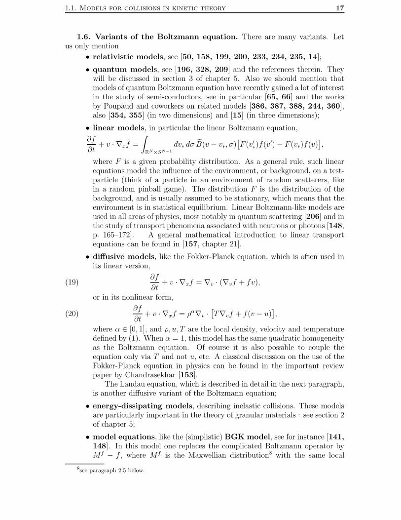
1.6. Variants of the Boltzmann equation. There are many variants. Letus only mention
• relativistic models, see [50, 158, 199, 200, 233, 234, 235, 14];
• quantum models, see [196, 328, 209] and the references therein. Theywill be discussed in section 3 of chapter 5. Also we should mention thatmodels of quantum Boltzmann equation have recently gained a lot of interestin the study of semi-conductors, see in particular [65, 66] and the worksby Poupaud and coworkers on related models [386, 387, 388, 244, 360],also [354, 355] (in two dimensions) and [15] (in three dimensions);
• linear models, in particular the linear Boltzmann equation,
∂f
∂t+ v · ∇xf =
∫
RN×SN−1
dv∗ dσ B(v − v∗, σ)[F (v′∗)f(v′)− F (v∗)f(v)
],
where F is a given probability distribution. As a general rule, such linearequations model the influence of the environment, or background, on a test-particle (think of a particle in an environment of random scatterers, likein a random pinball game). The distribution F is the distribution of thebackground, and is usually assumed to be stationary, which means that theenvironment is in statistical equilibrium. Linear Boltzmann-like models areused in all areas of physics, most notably in quantum scattering [206] and inthe study of transport phenomena associated with neutrons or photons [148,p. 165–172]. A general mathematical introduction to linear transportequations can be found in [157, chapter 21].
• diffusive models, like the Fokker-Planck equation, which is often used inits linear version,
(19)∂f
∂t+ v · ∇xf = ∇v · (∇vf + fv),
or in its nonlinear form,
(20)∂f
∂t+ v · ∇xf = ρα∇v ·
[T∇vf + f(v − u)
],
where α ∈ [0, 1], and ρ, u, T are the local density, velocity and temperaturedefined by (1). When α = 1, this model has the same quadratic homogeneityas the Boltzmann equation. Of course it is also possible to couple theequation only via T and not u, etc. A classical discussion on the use of theFokker-Planck equation in physics can be found in the important reviewpaper by Chandrasekhar [153].
The Landau equation, which is described in detail in the next paragraph,is another diffusive variant of the Boltzmann equation;
• energy-dissipating models, describing inelastic collisions. These modelsare particularly important in the theory of granular materials : see section 2of chapter 5;
• model equations, like the (simplistic) BGK model, see for instance [141,148]. In this model one replaces the complicated Boltzmann operator byMf − f , where M f is the Maxwellian distribution8 with the same local
8see paragraph 2.5 below.

18 CHAPTER 1. GENERAL PRESENTATION
density, velocity and temperature than f . Also variants are possible, forinstance multiplying this operator by the local density ρ...
Another very popular model equation for mathematicians is the Kacmodel [283]. It is a one-dimensional caricature of the Boltzmann equationwhich retains some of its interesting features. The unknown is a time-dependent probability measure f on R, and the equation reads
(21)∂f
∂t=
1
2π
(∫
R
dv∗
∫ 2π
0
dθ f ′f ′∗
)− f,
where (v′, v′∗) is obtained from (v, v∗) by a rotation of angle θ in the planeR
2. This model preserves mass and kinetic energy, but not momentum;
• discrete-velocity models : these are approximations of the Boltzmannequation where particles are only allowed a finite number of velocities. Theyare used in numerical analysis, but their mathematical study is (or once was)a popular topic. About them we shall say nothing; references can be foundfor instance in [230, 141, 148] and also in the survey papers [384, 62].Among a large number of works, we only mention the original contributionsby Bony [94, 95], Tartar [416, 417], and the consistency result by Bobylevet al [367], for the interesting number-theoretical issues that this paper hasto deal with.
We note [148, p. 265] that discrete-velocity models were once believedby physicists to provide miraculously efficient numerical codes for simulationof hydrodynamics. But these hopes have not been materialized...
Also some completely unrealistic discrete-velocity equations have beenstudied as simplified mathematical models, without caring whether theywould approximate or not the true Boltzmann equation. These modelssometimes have no more than two or three velocities ! Some well-knownexamples are the Carleman equation, with two velocities, the Broadwellmodel, with four velocities in the plane, or the Cabannes equation withfourteen velocities. For instance the Carleman equation reads
(22)
∂f1
∂t+∂f1
∂x= f 2
−1 − f 21 ,
∂f−1
∂t− ∂f−1
∂x= f 2
1 − f 2−1.
For a study of these models see [230, 384, 141, 148, 60, 61, 108, 25]and references included. Of course, these models are so oversimplified9 thatthey cannot be considered seriously from the physical point of view, evenif one may expect that they keep some relevant features of the Boltzmannequation. By the way, as noticed by Uchiyama [432], the Broadwell modelcannot be derived from a fictitious system of deterministic four-velocity par-ticles (“diamonds”) in the plane, see [149, Appendix 4C]. Only at the priceof some extra stochasticity assumption can the derivation be fixed [117].
All the abovementioned models should be considered with appropriate boundaryconditions. These conditions can also be replaced by the effect of a confinement
9As a word of caution, we should add that even if they are so simplified, their mathematical analysisis not trivial at all, and many problems in the field still remain open.

1.1. Models for collisions in kinetic theory 19
potential V (x) : this means that there is a macroscopic force of the form F (x) =−∇V (x) acting on the system.
Finally, it is important to note that Boltzmann’s model is obtained as a result ofthe assumption of localized interaction; in particular, it does not take into account apossible interaction of long (macroscopic) range which would result in a macroscopicmean-field force, typically
F (x) = −∇Φ(x), Φ(x) = ρ ∗x φ,where φ is the interaction potential and ρ the local density. The modelling of theinteraction by such a coupled force is called a Vlasov description.
When should one prefer a Vlasov, or a Boltzmann description ? A dimensionalanalysis by Bobylev and Illner [88] shows that for inverse-power forces like 1/rs, andunder natural scaling assumptions,
• for s > 3, the Boltzmann term should prevail on the mean-field term;
• for s < 3, the Boltzmann term should be negligible in front of the mean-fieldterm.
The separating case, s = 3, is the so-called Manev interaction [88, 279].There are subtle questions here, which are not yet fully understood, even at
a formal level. Also the uniqueness of the relevant scaling is not clear. From aphysicist’s point of view, however, it is generally accepted that a good descriptionis obtained by adding up the effects of a mean-field term and those of a Boltzmanncollision operator, with suitable dimensional coefficients.
Another way to take into account interactions on a macroscopically significantscale is to use a description a la Povzner. In this model (see for instance [389]),particles interact through delocalized collisions, so that the corresponding Boltz-mann operator is integrated with respect to the position y of the test particle, andreads
(23)
∫
RNx
dy
∫
RNv
dv∗ B(v − v∗, x− y
)[f(y, v′∗)f(x, v′)− f(y, v∗)f(x, v)
].
Note that the kernel B now depends on x − y. On the other hand, there is nocollision parameter σ any more, the outgoing velocities being uniquely determined bythe positions x, y and the ingoing velocities v′, v′∗. It was shown by Cercignani [140]that this type of equations could be retrieved as the limit of a large stochastic systemof “soft spheres”.
A related model is the Enskog equation for dense gases, which has never beenclearly justified. It resembles eq. (23) but the multiplicity of the integral is 2N − 1instead of 2N , because there is no integration over the distance |x − y|. Mathe-matical studies of the Enskog model have been performed by Arkeryd, Arkeryd andCercignani [24, 27, 28] — in particular, reference [24] provides well-posedness andregularity under extremely general assumptions (large data, arbitrary dimension) bya contraction method. See paragraph 2.1 in chapter 5 for an inelastic variant whichis popular in the study of granular material.
The study of these models is interesting not only in itself, but also becausenumerical schemes always have to perform some delocalization to simulate the effectof collisions. This explains why the results in [140] are very much related to some of

20 CHAPTER 1. GENERAL PRESENTATION
the mathematical justifications for some numerical schemes, as performed in [453,396].
1.7. Collisions in plasma physics. The importance and complexity of inter-action processes in plasma physics justifies that we devote a special paragraph tothis topic. A plasma, generally speaking, is a gas of (partially or totally) ionizedparticles. However, this term encompasses a huge variety of physical situations :the density of a plasma can be extremely low or extremely high, the pressures canvary considerably, and the proportion of ionized particles can also vary over severalorders of magnitude. Nonelastic collisions, recombination processes may be very im-portant. We do not at all try to make a precise description here, and refer to classicaltextbooks such as Balescu [46], Delcroix and Bers [164], the very nice survey byDecoster in [160], or the numerous references that can be found therein. All of thesesources put a lot of emphasis on the kinetic point of view, but [160] and [164] arealso very much concerned with fluid descriptions. A point which should be madenow, is that the classical collisional kinetic theory of gases a priori applies whenthe density is low (we shall make this a little bit more precise later on) and whennonelastic processes can be neglected.
Even taking into account only elastic interactions, there are a number of processesgoing on in a plasma : Maxwell-type interactions between ions and neutral particles,Van der Waals forces between neutral particles, etc. However, the most importantfeature, both from the mathematical and the physical point of view, is the presenceof Coulomb interactions between charged particles. The basic model for theevolution of the density of such particles is the Vlasov-Poisson equation
(24)∂f
∂t+ v · ∇xf + F (x) · ∇vf = 0,
F = −∇V, V =e2
4πε0r∗x ρ, ρ(t, x) =
∫f(t, x, v) dv.
For simplicity, here we have written this equation for only one species of particles,and also we have not included the effect of a magnetic field, which leads to the Vlasov-Maxwell system (see for instance [191]). We have kept the physical parameters e =charge of the particle and ε0 = permittivity of vacuum for the sake of a shortdiscussion about scales.
Even though this is not the topic of this review paper, let us say just a few wordson the Vlasov-Poisson equation. Its importance in plasma physics (including astro-physics) cannot be overestimated, and thousands of papers have been devoted toits study. We only refer to the aforementioned textbooks, together with the famoustreatise by Landau and Lipschitz [304]. From the mathematical point of view, thebasic questions of existence, uniqueness and (partial) regularity of the solution tothe Vlasov equation have been solved at the end of the eighties, see in particularPfaffelmoser [382], DiPerna and Lions [191], Lions and Perthame [318], Schaef-fer [402]. Reviews can be found in Glassey [233] and Bouchut [96]. Stability, and(what is more interesting !) instability of several classes of equilibrium distributionsto the Vlasov-Poisson equation have recently been the object of a lot of studies byGuo and Strauss [264, 265, 266, 267, 268]. Several important questions, how-ever, have not been settled, like the derivation of the Vlasov-Poisson equation fromparticle systems (see Spohn [410] and Neunzert [356] for related topics) and theexplanation of the famous and rather mysterious Landau damping effect.
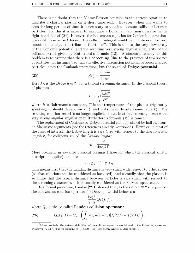
1.1. Models for collisions in kinetic theory 21
There is no doubt that the Vlasov-Poisson equation is the correct equation todescribe a classical plasma on a short time scale. However, when one wants toconsider long periods of time, it is necessary to take into account collisions betweenparticles. For this it is natural to introduce a Boltzmann collision operator in theright-hand side of (24). However, the Boltzmann equation for Coulomb interactionsdoes not make sense ! Indeed, the collision integral would be infinite even for verysmooth (or analytic) distribution functions10. This is due to the very slow decayof the Coulomb potential, and the resulting very strong angular singularity of thecollision kernel given by Rutherford’s formula (12). A standard remedy to thisproblem is to assume that there is a screening (due to the presence of two speciesof particles, for instance), so that the effective interaction potential between chargedparticles is not the Coulomb interaction, but the so-called Debye potential
(25) φ(r) =e−r/λD
4πε0r.
Here λD is the Debye length, i.e. a typical screening distance. In the classical theoryof plasmas,
λD =
√ε0kT
ρe2,
where k is Boltzmann’s constant, T is the temperature of the plasma (rigorouslyspeaking, it should depend on x...) and ρ its mean density (same remark). Theresulting collision kernel is no longer explicit, but at least makes sense, because thevery strong angular singularity in Rutherford’s formula (12) is tamed.
The replacement of Coulomb by Debye potential can be justified by half-rigorous,half-heuristic arguments (see the references already mentioned). However, in most ofthe cases of interest, the Debye length is very large with respect to the characteristiclength r0 for collisions, called the Landau length :
r0 =e2
4πε0kT.
More precisely, in so-called classical plasmas (those for which the classical kineticdescription applies), one has
r0 ρ−1/3 λD.
This means first that the Landau distance is very small with respect to other scales(so that collisions can be considered as localized), and secondly that the plasma isso dilute that the typical distance between particles is very small with respect tothe screening distance, which is usually considered as the relevant space scale.
By a formal procedure, Landau [291] showed that, as the ratio Λ ≡ 2λD/r0 →∞,the Boltzmann collision operator for Debye potential behaves as
log Λ
2πΛQL(f, f),
where QL is the so-called Landau collision operator :
(26) QL(f, f) = ∇v ·(∫
R3
dv∗ a(v − v∗)[f∗(∇f)− f(∇f)∗]
).
10More precisely, the natural definition of the collision operator would lead to the following nonsense :whatever f , Q(f, f) is an element of −∞, 0, +∞, see [450, Annex I, Appendix A].

22 CHAPTER 1. GENERAL PRESENTATION
Here a(z) is a symmetric (degenerate) nonnegative matrix, proportional to the or-thogonal projection onto z⊥ :
(27) aij(z) =L
|z|
[δij −
zizj|z|2
],
and L is a dimensional constant.The resulting equation is the Landau equation. In adimensional units, it could
be written as
(28)∂f
∂t+ v · ∇xf + F (x) · ∇vf = QL(f, f).
Many mathematical and physical studies also consider the simplified case when onlycollisions are present, and the effect of the mean-field term is not present. However,the collision term, normally, should be considered only as a long-time correction tothe mean-field term.
We now present a variant of the Landau equation, which appears when onereplaces the function L/|z| in (27) by |z|2, so that
(29) aij(z) = |z|2δij − zizj.This approximation is called “Maxwellian”. It is not realistic from the physical pointof view, but has become popular because it leads to simpler mathematical propertiesand useful tests for numerical simulations.
Under assumption (29), a number of algebraic simplifications arise in the Landauoperator (26); since they are independent on the dimension, we present them inarbitrary dimension N ≥ 2. Without loss of generality, choose an orthonormal basisof R
N in such a way that∫
RN
f dv = 1,
∫
RN
fv dv = 0,
∫
RN
f |v|2 dv = N
(unit mass, zero mean velocity, unit temperature), and assume moreover that∫
RN
fvivj dv = Tiδij
(the Ti’s are the directional temperatures; of course∑
i Ti = N). Then the Landauoperator with matrix (29) can be rewritten as
(30)∑
i
(N − Ti)∂iif + (N − 1)∇ · (fv) + ∆Sf.
Here ∆S stands for the Laplace-Beltrami operator,
∆Sf =∑
ij
(|v|2δij − vivj)∂ijf − (N − 1)v · ∇vf,
i.e. a diffusion on centered spheres in velocity space. Thus the Landau operatorlooks like a nonlinear Fokker-Planck type operator, with some additional isotropi-sation effect due to the presence of the Laplace-Beltrami operator. The diffusion isenhanced in directions where the temperature is low, and slowed down in directionswhere the temperature is high : this is normal, because in the end the temperaturealong all directions should be the same.
Formulas like (30) show that in the isotropic case, and under assumption (29), thenonlinear Landau equation reduces (in a well-chosen orthonormal basis) to the linearFokker-Planck equation ! By this remark [447] one can construct many explicit

1.1. Models for collisions in kinetic theory 23
solutions (which generalize the ones in [296]). These considerations explain whythe Maxwellian variant of the Landau equation has become a popular test case innumerical analysis [106].
Let us now review other variants of the Landau equation. First of all, thereare relativistic and quantum versions of it [304]. For a mathematically-orientedpresentation, see for instance [298]. There are also other, more sophisticated mod-els for collisions in plasmas : see for instance [164, section 13.6] for a syntheticpresentation. The most famous of these models is the so-called Balescu-Lenardcollision operator, whose complexity is just frightening for a mathematician. Itsexpression was established by Bogoljubov [90] via a so-called BBGKY-type hierar-chy, and later put by Lenard under the form that we give below. On the other hand,Balescu [46, 47] derived it as part of his general perturbative theory of approxima-tion of the Liouville equation for many particles. Just as the Landau operator, theBalescu-Lenard operator is in the form
(31)∑
ij
∂
∂vi
∫
R3
dv∗ aij(v, v∗)
(f∗∂f
∂vj− f ∂f∗
∂v∗j
),
but now the matrix aij depends on f in a strongly nonlinear way :
(32) aij(v, v∗) =
∫
k∈R3, |k|≤Kmax
δ[k · (v − v∗)]kikj|k|4
1
|ε|2 dk,
where ε is the “longitudinal permittivity” of the plasma,
ε = 1− 8π
|k|2∫
1
k · (v − v∗)− i0k · (∇f)∗ dv∗.
Here δ is the Dirac measure at the origin, and
1
x− i0 = limε→0+
1
x− iε = P(
1
x
)+ iπδ
is a complex-valued distribution on the real line (P stands for the Cauchy principalpart). Moreover, Kmax is a troncature parameter (whose value is not very clearlydetermined) which corresponds to values of the deviation angles beyond which col-lisions cannot be considered grazing. This is not a Debye cut !
Contrary to Landau, Balescu and Lenard derived the operator QL (26) as anapproximation of (31). To see the link between these two operators, let us setk = µω, µ ≥ 0, ω ∈ S2; then one can rewrite (32) as
(33)
∫
S2
dω δ[ω · (v − v∗)]ωiωj(∫ Kmax
0
dµ
µ|ε|2).
But ∫
S2
dω δ(ω · z)ωiωj =π
|z|
(δij −
zizj|z|2
).
So one can replace the operator (31) by the Landau collision operator if one admitsthat the integral in dµ in (33) depends very little on v, v∗, ω. Under this assumption,it is natural to replace f by a Maxwellian11, and one finds for this integral anexpression of the form 1 + (µ2
D)/µ2, where µD has the same homogeneity as theinverse of a Debye length. Then one can perform the integration; see Decoster [160]for much more details.
11This is the natural statistical equilibrium, see paragraph 2.5.

24 CHAPTER 1. GENERAL PRESENTATION
In spite of its supposed accuracy, the interest of the Balescu-Lenard model isnot so clear. Due to its high complexity, its numerical simulation is quite tricky.And except in very particular situations, apparently one gains almost nothing, interms of physical accuracy of the results, by using it as a replacement for the Landauoperator. In fact, it seems that the most important feature of the Balescu-Lenardoperator, to this date, is to give a theoretical basis to the use of the Landau operator !
There exist in plasma physics some even more complicated models, such as thosewhich take into account magnetic fields (Rostoker operator, see for instance [465]and the references therein). We refrain from writing up the equations here, since thiswould require several pages, and they seem definitely out of reach of a mathematicaltreatment for the moment... We also mention the simpler linear Fokker-Planckoperator for Coulomb interaction, derived by Chandrasekhar. This is a linearoperator of Landau-type, which describes the evolution of a test-particle interactingwith a “bath” of Coulomb particles in thermal equilibrium. A formula for it is givenin Balescu [46, paragraph 37], in terms of special functions.
1.8. Physical validity of the Boltzmann equation. Experience has shownthat the Boltzmann equation and its variants realistically describe phenomena whichoccur in dilute atmosphere, in particular aeronautics at high altitude, or interactionsin dilute plasmas. In many situations, predictions based on the Navier-Stokes equa-tion are not accurate for low densities; a famous historical example is provided bythe so-called Knudsen minimum effect in a Poiseuille flow [148, p. 99] : if the differ-ence of pressure between the entrance and the exit of a long, narrow channel is keptfixed, then the flow rate through a cross-section of this channel is not a monotonicfunction of the average pressure, but exhibits a minimum for a certain value of thisparameter. This phenomenon, established experimentally by Knudsen, remainedcontroversial till the 1960’s.
Also the Boltzmann equation cannot be replaced by fluid equations when it comesto the study of boundary layers (Knudsen layer, Sone sublayer due to curvature...)and the gas-surface interaction.
Nowadays, with the impressive development of computer power, it is possibleto perform very precise numerical simulations which seem to fully corroborate thepredictions based on the Boltzmann equation — within the right range of physicalparameters, of course.
All these questions are discussed, together with many numerical simulations andexperiments, in the recent broad-audience survey book by Cercignani [148] (see alsothe review paper [136] by the same author in the present volume).
2. Mathematical problems in collisional kinetic theory
In this section, we try to define the most interesting mathematical problemswhich arise in the study of Boltzmann-like equations. At this point we should makeit clear that the Boltzmann equation can be studied for the sake of its applications todilute gases, but also as one of the most basic and famous models for nonequilibriumstatistical mechanics.
2.1. Mathematical validity of the Boltzmann equation. In the last para-graph, we have mentioned that, in the right range of physical parameters, the phys-ical validity of the Boltzmann equation now seems to be beyond any doubt. Onthe other hand, the mathematical validity of the Boltzmann equation poses a more
1.2. Mathematical problems in collisional kinetic theory 25
challenging problem. For the time being, it has been investigated only for the hard-sphere model.
Let us give a short description of the problem in the case of hard spheres. Butbefore that, we add a word of caution about the meaning of “mathematical valid-ity” : it is not a proof that the model is the right one in a certain range of physicalparameters (whatever this may mean). It is only a rigorous derivation of the model,in a suitable asymptotic procedure, from another model, which is conceptually sim-pler but contains more information (typically : the positions of all the particles,as opposed to the density of particles). Of course, the Boltzmann equation, justlike many models, can be derived either by mathematical validation, or by directmodelling assumptions, and the second approach is more arbitrary, less interestingfrom the mathematical point of view, but not less “respectable” if properly imple-mented ! This is why, for instance, Truesdell [430] refuses to consider the problemof mathematical validity of the Boltzmann equation.
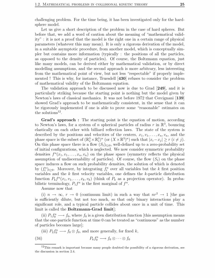
The validation approach to be discussed now is due to Grad [249], and it isparticularly striking because the starting point is nothing but the model given byNewton’s laws of classical mechanics. It was not before 1972 that Cercignani [139]showed Grad’s approach to be mathematically consistent, in the sense that it canbe rigorously implemented if one is able to prove some “reasonable” estimates onthe solutions12.
Grad’s approach : The starting point is the equation of motion, accordingto Newton’s laws, for a system of n spherical particles of radius r in R
3, bouncingelastically on each other with billiard reflection laws. The state of the system isdescribed by the positions and velocities of the centers, x1, v1, . . . , xn, vn, and thephase space is the subset of (R3
x×R3v)n (or (X×R
3)n) such that |xi−xj| ≥ r (i 6= j).On this phase space there is a flow (St)t≥0, well-defined up to a zero-probability setof initial configurations, which is neglected. We now consider symmetric probabilitydensities fn(x1, v1, . . . , xn, vn) on the phase space (symmetry reflects the physicalassumption of undiscernability of particles). Of course, the flow (St) on the phasespace induces a flow on such probability densities, the solution of which is denotedby (fnt )t≥0. Moreover, by integrating fnt over all variables but the k first positionvariables and the k first velocity variables, one defines the k-particle distributionfunction Pkf
n(x1, v1, . . . , xk, vk) (think of Pk as a projection operator). In proba-bilistic terminology, P1f
n is the first marginal of fn.Assume now that
(i) n → ∞, r → 0 (continuum limit) in such a way that nr2 → 1 [the gasis sufficiently dilute, but not too much, so that only binary interactions play asignificant role, and a typical particle collides about once in a unit of time. Thislimit is called the Boltzmann-Grad limit];
(ii) P1fn0 −→ f0, where f0 is a given distribution function [this assumption means
that the one-particle function at time 0 can be treated as “continuous” as the numberof particles becomes large];
(iii) P2fn0 −→ f0 ⊗ f0, and more generally, for fixed k,
(34) Pkfn0 −→ f0 ⊗ · · · ⊗ f0
12This remark is important because many people doubted the possibility of a rigorous derivation, seethe discussion in section 2.4.
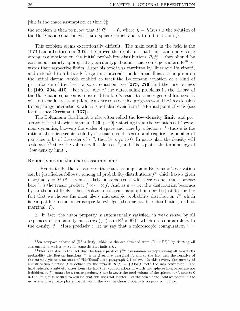
26 CHAPTER 1. GENERAL PRESENTATION
[this is the chaos assumption at time 0];
the problem is then to prove that P1fnt −→ ft, where ft = ft(x, v) is the solution of
the Boltzmann equation with hard-sphere kernel, and with initial datum f0.
This problem seems exceptionally difficult. The main result in the field is the1973 Lanford’s theorem [292]. He proved the result for small time, and under somestrong assumptions on the initial probability distributions Pkf
n0 : they should be
continuous, satisfy appropriate gaussian-type bounds, and converge uniformly13 to-wards their respective limits. Later his proof was rewritten by Illner and Pulvirenti,and extended to arbitrarily large time intervals, under a smallness assumption onthe initial datum, which enabled to treat the Boltzmann equation as a kind ofperturbation of the free transport equation: see [275, 276] and the nice reviewsin [149, 394, 410]. For sure, one of the outstanding problems in the theory ofthe Boltzmann equation is to extend Lanford’s result to a more general framework,without smallness assumption. Another considerable progress would be its extensionto long-range interactions, which is not clear even from the formal point of view (seefor instance Cercignani [137]).
The Boltzmann-Grad limit is also often called the low-density limit, and pre-sented in the following manner [149, p. 60] : starting from the equations of Newto-nian dynamics, blow-up the scales of space and time by a factor ε−1 (thus ε is theratio of the microscopic scale by the macroscopic scale), and require the number ofparticles to be of the order of ε−2, then let ε go to 0. In particular, the density willscale as ε2/3 since the volume will scale as ε−3, and this explains the terminology of“low density limit”.
Remarks about the chaos assumption :
1. Heuristically, the relevance of the chaos assumption in Boltzmann’s derivationcan be justified as follows : among all probability distributions fn which have a givenmarginal f = P1f
n, the most likely, in some sense which we do not make precisehere14, is the tensor product f ⊗ · · · ⊗ f . And as n→∞, this distribution becomesby far the most likely. Thus, Boltzmann’s chaos assumption may be justified by thefact that we choose the most likely microscopic probability distribution f n whichis compatible to our macroscopic knowledge (the one-particle distribution, or firstmarginal, f).
2. In fact, the chaos property is automatically satisfied, in weak sense, by allsequences of probability measures (fn) on (R3 × R
3)n which are compatible withthe density f . More precisely : let us say that a microscopic configuration z =
13on compact subsets of (R3 × R3)k
6=, which is the set obtained from (R3 × R3)k by deleting all
configurations with xi = xj for some distinct indices i, j.14This is related to the fact that the tensor product f⊗n has minimal entropy among all n-particles
probability distribution functions fn with given first marginal f , and to the fact that the negative ofthe entropy yields a measure of “likelihood”, see paragraph 2.4 below. [In this review, the entropy ofa distribution function f is defined by the formula H(f) =
R
f log f ; note the sign convention.] Forhard spheres, a subtlety arises from the fact that configurations in which two spheres interpenetrate areforbidden, so fn cannot be a tensor product. Since however the total volume of the spheres, nr3, goes to 0in the limit, it is natural to assume that this does not matter. On the other hand, contact points in then-particle phase space play a crucial role in the way the chaos property is propagated in time.

1.2. Mathematical problems in collisional kinetic theory 27
(x1, v1, . . . , xn, vn) ∈ (R3x × R
3v)n is admissible if its empirical density,
ωz =1
n
n∑
i=1
δ(xi,vi),
is a good approximation to the density f(x, v) dx dv, and let (f n)n∈N be a sequence ofsymmetric probability densities on (R3
x×R3v)n respectively, such that the associated
measures µn give very high probability to configurations which are admissible. In amore precise writing, we require that for every bounded continuous function ϕ(x, v)on R
3 × R3, and for all ε > 0,
µn[z ∈ (R3
x × R3v)n;∣∣∣∫
R3x×R3
v
ϕ(x, v)[ωz(dx dv)− f(t, x, v) dx dv
]∣∣∣ > ε
]−−−→n→∞
0.
Then, (fn) satisfies the chaos property, in weak sense [149, p. 91] : for any k ≥ 1,
Pkfn −−−→
n→∞f⊗k
in weak-∗ measure sense. This statement expresses the fact that f n is automaticallyclose to the tensor product f⊗n in the sense of weak convergence of the marginals.However, weak convergence is not sufficient to derive the Boltzmann equation, be-cause of the problem of localization of collisions. Therefore, in Lanford’s theoremone imposes a stronger (uniform) convergence of the marginals, or strong chaosproperty.
3. This is the place where probability enters the Boltzmann equation : viathe initial datum, i.e. the probability density (fn) ! According to [149, p. 93],the conclusion of Lanford’s theorem can be reformulated as follows : for all timet > 0, if fnt is obtained from fn0 by transportation along the characteristics of themicroscopic dynamics, and if µnt is the probability measure on (R3
x × R3v)n whose
density is given by fnt , then for all ε > 0, and for all bounded, continuous functionϕ(x, v) on R
3x × R
3v,
µnt
[z ∈ (R3
x × R3v)n;∣∣∣∫
R3x×R3
v
ϕ(x, v)[ωz(dx dv)− ft(x, v) dx dv
]∣∣∣ > ε
]−−−→n→∞
0,
where ft is the solution to the Boltzmann equation with initial datum f0. In termsof µn :
µn[
z ∈ (R3x × R
3v)n;∣∣∣∫
R3x×R3
v
ϕ(x, v)[ωStz(dx dv)− ft(x, v) dx dv
]∣∣∣ > ε
]−−−→n→∞
0.
In words : for most initial configurations, the evolution of the density under the mi-croscopic dynamics is well approximated by the solution to the Boltzmann equation.Of course, this does not rule out the existence of “unlikely” initial configurations forwhich the solution of the Boltzmann equation is a very bad approximation of theempirical measure.
4. If the chaos property is the crucial point behind the Boltzmann derivation,then one should expect that it propagates with time, and that
(35) ∀t > 0, Pkfnt → ft ⊗ · · · ⊗ ft.
However, this propagation property only holds in a weak sense. Even if the con-vergence is strong (say, uniform convergence of all marginals) in (34), it has to beweaker in (35), say almost everywhere, see the discussion in Cercignani et al. [149].

28 CHAPTER 1. GENERAL PRESENTATION
The reason for this weakening is the appearance of microscopic correlations (un-der evolution by the microscopic, reversible dynamics). In particular, if the initialmicroscopic datum is “very likely”, this does not imply at all that the microscopicdatum at later times should be very likely ! On the contrary, it should present a lotof correlations...
5. In fact, one has to be extremely cautious when handling (35). To illustratethis, let us formally show that for t > 0 the approximation
(36) P2fnt (x, v; y, w) ' ft(x, v)ft(y, w)
cannot be true in strong sense, uniformly in all variables15, as n → ∞ (the symbol' here means “approaches, in L∞ norm, uniformly in all variables x, y, v, w, asn → ∞”). Indeed, assume that (36) holds true uniformly in x, y, v, w, and choosey = x+rσ, 〈v−w, σ〉 > 0, i.e. an ingoing collisional configuration in the two-particlephase space. Then, presumably
(37) P2fnt (x, v; x+ rσ, w) ' ft(x, v)ft(x+ rσ, w) ' ft(x, v)ft(x, w)
as n→∞. But from the specular reflection condition, for any t > 0,
P2fnt (x, v; x+ rσ, w) = P2f
nt (x, v′; x+ rσ, w′),
where v′ and w′ are post-collisional velocities,
v′ = v − 〈v − w, σ〉 σ, w′ = w + 〈v − w, σ〉 σ.Applying (36) again, this would result in
P2fnt (x, v; x+ rσ, w) = P2f
nt (x, v′; x+ rσ, w′) ' ft(x, v
′)ft(x, w′),
which is not compatible with (37) (unless ft solves eq. (53) below). This contra-diction illustrates the fact that (36) cannot be propagated by the dynamics of hardspheres. It is actually property (37), sometimes called one-sided chaos, which isused in the derivation of the Boltzmann equation, and which should be propagatedfor positive times : it means that the velocities of particles which are just aboutto collide are not correlated. But it is a very difficult problem to handle eq. (37)properly, because it involves the restriction of fn to a manifold of codimension 1,and may be violated even for initial data which satisfy the conditions of Lanford’stheorem ! So an appropriate generalized sense should be given to (37). Lanford’sargument cleverly avoids any discussion of (37), and only assumes (36) at time 0, theapproximation being uniform outside collisional configurations. So he plainly avoidsdiscussing one-sided chaos, and does not care what is propagated for positive times,apart from weak chaos16. To sum up : the physical derivation of the Boltzmannequation is based on the propagation of one-sided chaos, but no one knows how thisproperty should be expressed mathematically — if meaningful at all.
An easier variant of the validation problem is the derivation of linear transportequations describing the behavior of a Lorentz gas : a test-particle in a randompinball game, with scatterers randomly distributed according to (say) a Poisson law.Under a suitable scaling, the law of this test-particle converges towards the solutionof a linear Boltzmann equation, as was first formalized by Gallavotti [226], beforeseveral improvements appeared [409, 91]. See Pulvirenti [394] for a review and
15constrained by |x − y| ≥ r.16This is possible because he uses a perturbative proof, based on an iterative Duhamel formula, in
which everything is expressed in terms of the initial datum...

1.2. Mathematical problems in collisional kinetic theory 29
introduction of the subject. The convergence actually holds true for almost all (inthe sense of Poisson measure) fixed configuration of scatterers, but fails for certainspecific configurations, for instance a periodic array, as shown in Bourgain, Golseand Wennberg [102]. We also note that Desvillettes and Pulvirenti [179] are able torigorously justify the linear Boltzmann equation for some interactions with infiniterange.
Kac’s approach : To conclude this paragraph, we mention another line ofapproach towards the mathematical justification of the Boltzmann equation. It goesvia the construction of some many-particle stochastic system, such that the firstmarginal of its law at a given time t should be an approximation of the solution tothe Boltzmann equation if the initial datum is chaotic. This subject was initiatedby Kac17 [283], and developed by Sznitman [412] in connection with the problem ofpropagation of chaos. Recent progress on this have been achieved by Graham andMeleard [256, 344].
The main conceptual difference between both approaches lies in the momentwhere probability is introduced, and irreversibility18 as well. In Lanford’s approach,the starting point is a deterministic particle system; it is only the particular “chaotic”choice of the initial datum which leads to the macroscopic, irreversible Boltzmannequation in the limit. On the other hand, for Kac the microscopic particle system isalready stochastic and irreversible from the beginning. Then the main effect of thelimit is to turn a linear equation on a large n-particle phase space, into a nonlinearequation on a reduced, one-particle phase space.
Of course Kac’s approach is less striking than Grad’s, because the starting pointcontains more elaborate modelling assumptions, since stochasticity is already builtin. Kac formulated his approach in a spatially homogeneous19 setting, while thiswould be meaningless for Grad’s approach. In fact, it is as if Kac wanted to treatthe positions of the particles (which, together with ingoing velocities, determine theoutgoing velocities) as hidden probabilistic variables. Then, all the subtleties linkedto one-sided chaos can be forgotten, and it is sufficient to study just propagation of(weak) chaos.
Moreover, Kac’s approach becomes important when it comes to make an inter-pretation of the Monte Carlo numerical schemes which are often used to computeapproximate solutions of the Boltzmann equation. These schemes are indeed basedon large stochastic particle systems. See Pulvirenti [394, 453, 396] for referencesabout the study of these systems, in connection with the validation problem. We donot develop here on the problem of the rigorous justification of numerical schemes,but this topic is addressed in the companion review [136] by Cercignani.
2.2. The Cauchy problem. From the mathematical point of view, the veryfirst problem arising in the study of the Boltzmann equation is the Cauchy prob-lem : given a distribution function f0(x, v) on R
Nx × R
Nv (or X × R
Nv ), satisfying
appropriate and physically realistic assumptions, show that there exists a (unique)
17See paragraph 1.5 in chapter 5.18See paragraph 2.4.19See paragraph 5.2.
30 CHAPTER 1. GENERAL PRESENTATION
solution of
(38)
∂f
∂t+ v · ∇xf = Q(f, f),
f(0, ·, ·) = f0.
Needless to say, the Boltzmann equation seems impossible to solve explicitly20,except in some very particular situations : semi-explicit solutions by Bobylev [79],Bobylev and Cercignani [81]; self-similar solutions of infinite mass by Nikolskii,see [289, p. 286]; particular solutions in a problem of shear flow by Truesdell,see [430, chap. 14–15], some simple problems of modelling with a lot of symme-tries [148]... Explicit solutions are discussed in the review paper [207]. These exactsolutions are important in certain modelling problems, but they are exceptional.This justifies the study of a general Cauchy problem.
Of course, the question of the Cauchy problem should be considered as a prelimi-nary for a more detailed study of qualitative properties of solutions of the Boltzmannequation. The main qualitative properties in which one is interested are : smooth-ness and singularities, conservation laws, strict positivity, existence of Lyapunovfunctionals, long-time behavior, limit regimes. We shall come back on all of thisin the next chapters. As recalled in section 3, the properties of the solutions maydepend heavily on the form of the collision kernel.
As of this date, the Cauchy problem has still not received satisfactory answers.As we shall describe in section 5, there are several “competing” theories which eitherconcern (more or less) simplified cases, or are unable to answer the basic questionsone may ask about the solutions. Yet this problem has spectacularly advanced sincethe end of the eighties.
Another fundamental problem in many areas of modelling by Boltzmann equa-tion, as explained for instance in Cercignani [148], is the existence of stationarysolutions : given a box X, prove that there exists a (unique ?) stationary solutionof the Boltzmann equation in the box :
v · ∇xf = Q(f, f), x ∈ X, v ∈ RN
together with well-chosen boundary conditions (ideally, dictated by physical assump-tions).
The stationary problem has been the object of a lot of mathematical studies inthe past few years; see for instance [31, 25, 34, 36, 26, 37, 38]. We shall notconsider it here, except for a few remarks. This is first because the theory is lessdeveloped than the theory of the Cauchy problem, secondly because we wish to avoidthe subtle discussion of boundary conditions for weak solutions.
2.3. Maxwell’s weak formulation, and conservation laws. The change ofvariables (v, v∗, σ) −→ (v′, v′∗, k), with k = (v − v∗)/|v − v∗|, has unit Jacobian andis involutive. Since σ = (v′−v′∗)/|v′−v′∗|, one can abuse terminology by referring tothis change of variables as (v, v∗) −→ (v′, v′∗). It will be called the pre-postcollisionalchange of variables. As a consequence of microreversibility, it leaves the collisionkernel B invariant.
20Although no theorem of non-solvability has been proven !
1.2. Mathematical problems in collisional kinetic theory 31
The fact that this change of variable has unit Jacobian is not a general feature ofBoltzmann-like equations, actually it is false for energy-dissipating models21... Alsothe change of variables (v, v∗) −→ (v∗, v) is clearly involutive and has unit Jacobian.As a consequence, if ϕ is an arbitrary continuous function of the velocity v,
∫
RNv
Q(f, f)ϕdv =
∫
RN×RN
dv dv∗
∫
SN−1
dσ B(v − v∗, σ)(f ′f ′∗ − ff∗)ϕ
(39)
=
∫
RN×RN
dv dv∗
∫
SN−1
dσ B(v − v∗, σ)ff∗(ϕ′ − ϕ)(40)
=1
2
∫
RN×RN
dv dv∗
∫
SN−1
dσ B(v − v∗, σ)ff∗(ϕ′ + ϕ′
∗ − ϕ− ϕ∗).(41)
This gives a weak formulation for Boltzmann’s collision operator. From the mathe-matical point of view, it is interesting because expressions like (40) or (41) may bewell-defined in situations where Q(f, f) is not. From the physical point of view, itexpresses the change in the integral
∫f(t, x, v)ϕ(v) dv which is due to the action of
collisions. Actually, this formulation is so natural for a physicist, that equation (40)was written by Maxwell22 [335, eq. 3] before Boltzmann gave the explicit expressionof Q(f, f) !
Let f be a solution of the Boltzmann equation (8), set in the whole space RNx to
simplify. By the conservative properties of the transport operator, v · ∇x,
(42)d
dt
∫f(t, x, v)ϕ(v) dx dv =
∫Q(f, f)ϕdx dv,
and the right-hand side is just the x-integral of any one of the expressions in for-mulas (39)–(41). As an immediate consequence, whenever ϕ satisfies the functionalequation
(43) ∀(v, v∗, σ) ∈ RN × R
N × SN−1, ϕ(v′) + ϕ(v′∗) = ϕ(v) + ϕ(v∗)
then, at least formally,
d
dt
∫f(t, x, v)ϕ(v) dx dv = 0
along solutions of the Boltzmann equation. The words “at least formally” of coursemean that the preceding equations must be rigorously justified with the help of someintegrability estimates on the solutions to the Boltzmann equation.
It can be shown under very weak conditions23 [142, 29], [149, p. 36–42] that so-lutions to (43), as expected, are only linear combinations of the collision invariants :
ϕ(v) = 1, vi,|v|22, 1 ≤ i ≤ N.
21See section 2 in chapter 5.22Actually it is not so easy to recognize the Boltzmann equation in Maxwell’s notations !23This problem was first treated by Gronwall [259, 260] and Carleman [119] under stronger conditions.
Then people started to study it under weaker and weaker assumptions. Its interest lies not only in checkingthat there are no hidden conservation laws in the Boltzmann equation, but also in solving the importanteq. (53) below, for which simpler methods are however available.
32 CHAPTER 1. GENERAL PRESENTATION
This leads to the (formal) conservation laws of the Boltzmann equation,
d
dt
∫f(t, x, v)
1vi|v|22
dx dv = 0, 1 ≤ i ≤ N
meaning that the total mass, the total momentum and the total energy of the gasare preserved.
These conservation laws should hold true when there are no boundaries. In pres-ence of boundaries, conservation laws may be violated : momentum is not preservedby specular reflection, neither is energy if the gas is in interaction with a wall keptat a fixed temperature. See Cercignani [141, 148] for a discussion of general axiomsof the classical modelling of gas-surface interaction, and resulting laws.
If one disregards this possible influence of boundaries, then the preservation ofmass, momentum and energy under the action of the Boltzmann collision operatoris clearly the least that one can expect from a model which takes into account onlyelastic collisions. Yet, to this date, no mathematical theory has been able to justifythese simple rules at a sufficient level of generality. The problem is of course that toolittle is known about how well behaved are the solutions to the Boltzmann equation.Conservation of mass and momentum are no problem, but no one knows how toobtain an a priori estimate which would imply a little bit more integrability thanjust finite energy.
Another crucial topic for a fluid description is the validity of local conservationlaws, i.e. continuity equations obtained by integrating the Boltzmann equation withrespect to v only. With notations (1), these equations are
(44)
∂ρ
∂t+∇x · (ρu) = 0,
∂
∂t(ρu) +∇x ·
(∫
RN
fv ⊗ v dv)
= 0,
∂
∂t(ρ|u|2 +NρT ) +∇x ·
(∫
RN
f |v|2 v dv)
= 0.
At this moment, only the first of these equations has been proven in full general-ity [308].
2.4. Boltzmann’s H theorem and irreversibility. In this paragraph, wediscuss some of the most famous aspects of the Boltzmann equation. This willjustify a few digressions to make the topic as clear as possible.
Let us symmetrize the integral (39) once more, fully using all the symmetries ofthe collision operator. We obtain
(45)
∫Q(f, f)ϕdv = −1
4
∫dv dv∗ dσ B(v− v∗, σ)
(f ′f ′
∗− ff∗)(ϕ′ +ϕ′
∗−ϕ−ϕ∗).
We shall refer to this formula as Boltzmann’s weak formulation.

1.2. Mathematical problems in collisional kinetic theory 33
Without caring about integrability issues, we plug ϕ = log f into this equation,and use the properties of the logarithm, to find
(46)
∫
RN
Q(f, f) log f dv = −D(f),
where D is the entropy dissipation functional,
(47) D(f) =1
4
∫
R2N×SN−1
dv dv∗ dσ B(v − v∗, σ)(f ′f ′
∗ − ff∗)
logf ′f ′
∗ff∗≥ 0.
That D(f) ≥ 0 just comes from the fact that the function (X, Y ) 7−→ (X −Y )(logX − log Y ) is nonnegative.
Next, we introduce Boltzmann’s H functional,
(48) H(f) =
∫
RNx ×RN
v
f log f.
Of course, the transport operator −v · ∇x does not contribute in any change ofthe H functional in time24. As a consequence, if f = f(t, x, v) is a solution of theBoltzmann equation, then H(f) will evolve in time because of the effects of thecollision operator :
(49)d
dtH(f(t, ·, ·)
)= −
∫
RNx
D(f(t, x, ·)
)dx ≤ 0.
This is the famous Boltzmann’s H theorem : the H-functional, or entropy, isnonincreasing with time. This theorem is “proven” and discussed at length in Boltz-mann’s treatise [93]. Before commenting on its physical implications, let us give afew analytical remarks :
1. For certain simplified models of the Boltzmann equation, McKean [342] hasproven that the H-functional is, up to multiplicative and additive constants, theonly “local” (i.e. of the form
∫A(f)) Lyapunov functional.
2. There are some versions with boundary conditions; actually, it was empha-sized by Cercignani that the H theorem still holds true for a modified H-functional(including the temperature of the wall, for instance, if the wall is kept at fixed tem-perature) as soon as a certain number of general axioms are satisfied. See [141] forprecise statements.
3. The argument above, leading to formula (47), does not work for certainvariants of the Boltzmann equation, like mixtures. Actually Boltzmann had alsogiven a (false) proof in this case, and once the error was discovered, produced atotally obscure argument to fix it (see the historical references in [148]). As pointedout by Cercignani and Lampis [150], the most robust way to prove the H theoremis to use again Maxwell’s weak formulation, and to note that
(50)1
2
∫Bff∗ log
f ′f ′∗
ff∗dv dv∗ dσ =
1
2
∫Bff∗
(log
f ′f ′∗
ff∗− f ′f ′
∗ff∗
+ 1
)≤ 0,
because∫Q(f, f) dv = 0 and logX−X+1 ≤ 0. This line of proof can be generalized
to mixtures [148, paragraph 6.4] and other models.
24More generally, the transport operator does not contribute to any change of a functional of the formR
A(f) dxdv.
34 CHAPTER 1. GENERAL PRESENTATION
4. The Landau equation also satisfies a H theorem. The corresponding entropydissipation is (formally)
(51) DL(f) =1
2
∫
R3×R3
ff∗
∣∣∣∣√a(v − v∗)
(∇(log f)− [∇(log f)]∗
)∣∣∣∣2
dv dv∗.
What is the physical sense of Boltzmann’s H theorem ? First of all, we notethat the H functional should coincide with the usual entropy of physicists up toa change of sign. Also, it is a dynamical entropy, in the sense that is defined fornonequilibrium systems. Thus Boltzmann’s H theorem is a manifestation of thesecond law of thermodynamics (Clausius’ law) which states that the physical entropyof an isolated system should not decrease in time. In particular, it demonstrates thatthe Boltzmann model has some irreversibility built in. This achievement (producean analytical proof of the second law for some specific model of statistical mechanics)was one of the early goals of Boltzmann, and was later considered as one of his mostimportant contributions to statistical physics.
But the H theorem immediately raised a number of objections, linked to the factthat the starting point of the derivation of the Boltzmann equation is just classical,reversible mechanics — so where does the irreversibility come from ? Of course,since the existence of atoms was controversial at the time, Boltzmann’s constructionseemed very suspect... About the controversy between Boltzmann and opponents,and the way to resolve apparent contradictions in Boltzmann’s approach, one mayconsult [202, 284, 149, 293]. Here we shall explain in an informal way the mainarguments of the discussion, warning the reader that the following considerationshave not been put on a satisfactory mathematical basis.
Zermelo pointed out that Boltzmann’s theorem seemed to contradict the famousPoincare recurrence theorem25. Boltzmann replied that the scales of time on whichPoincare’s theorem applied in the present setting were much larger than the age ofthe universe, and therefore irrelevant. This answer is justified by the fact that theBoltzmann equation should be a good approximation of the microscopic dynamics,only on a time scale which depends on the actual number of particles — see thediscussion in the end of paragraph 2.5.
Then Loschmidt came out with the following paradox. Let be given a gas ofparticles, evolving from time 0 to time t0 > 0. At time t0, reverse all velocities andlet the gas evolve freely otherwise. If Boltzmann were right, the same Boltzmannequation should describe the behavior of the gas on both time intervals [0, t0] and[t0, 2t0]. Since the reversal of velocities does not change the entropy of a distributionfunction, the entropy at time 2t0 should be strictly less than the entropy at time 0.But, by time-reversibility of classical mechanics, at time 2t0 the system should beback to its initial configuration, which would be a contradiction... To this argumentBoltzmann is reported to have replied “Go on, reverse the velocities !”
The answer to Loschmidt’s paradox is subtle and has to do with the probabilis-tic content of the Boltzmann equation. Starting with the classical monograph byP. and T. Ehrenfest [202], it was understood that reversible microdynamics and
25For almost all choice of the initial datum, a conservative system with a compact phase space willalways come arbitrarily close to its initial configuration for large enough times. This theorem applies to asystem of n particles obeying the laws of classical mechanics, interacting via elastic collisions, enclosed ina box.
1.2. Mathematical problems in collisional kinetic theory 35
irreversible macrodynamics are not contradictory, provided that the right amountof probability is used in the interpretation of the macroscopic model. This view isvery well explained in the excellent book by Kac [284].
In the case of the Boltzmann derivation, everything seems deterministic : nei-ther the microscopic model, nor the macroscopic equation are stochastic. But theprobabilistic content is hidden in the choice of the initial datum. As we mentionedearlier26, with very high probability the Boltzmann equation gives a good approx-imation to the evolution of the density of the gas. And here randomness is in thechoice of the microscopic initial configuration, among all configurations which arecompatible with the density f (see paragraph 2.1 for more precise formulations). Butfor exceptional configurations which are not chaotic, the derivation of the Boltzmannequation fails.
Now comes the tricky point in Loschmidt’s argument. As we discussed in para-graph 2.1, the chaos property, in strong sense, is not preserved by the microscopic,reversible dynamics. What should be preserved is the one-sided chaos : ingoing colli-sional configurations are uncorrelated. More precisely, if the strong chaos assumptionholds true at initial time, then chaos should be true for ingoing configurations atpositive times, and for outgoing configurations at negative times.
So, reversing all velocities as suggested by Loschmidt is an innocent operationat the level of the limit one-particle distribution (which has forgotten about cor-relations), but by no means at the level of the microscopic dynamics (which keepsall correlations in mind). It will transform a configuration which is chaotic as faras ingoing velocities are concerned, into a configuration which is chaotic as far asoutgoing velocities are concerned27... Then, the microscopic dynamics will preservethis property that outgoing velocities are not correlated, and, by repeating the stepsof the derivation of the Boltzmann equation, we find that the correct equation, todescribe the gas from time t0 on, should be the negative Boltzmann equation (witha minus sign in front of the collision operator). Therefore in Loschmidt’s argument,of course the entropy is unchanged at time t0, but then it should start to increase,and be back at its original value at time 2t0.
At the moment, a fully satisfactorily mathematical discussion of Loschmidt’sparadox is not possible, since we do not know what one-sided chaos should reallymean, mathematically speaking. But one can check, as is done in [149, section 4.7],that strong chaos28 is not propagated in time — so that it will be technically im-possible to repeat Lanford’s argument when taking as initial datum the microscopicconfiguration at time t0, be it before or after reversal of velocities.
With this in mind, one also easily answers to the objection, why would the Boltz-mann equation select a direction of time ? Actually, it does not29, and this can beseen by the fact that if strong30 chaos is assumed at initial time, then the correctequation should be the Boltzmann equation for positive times, and the negativeBoltzmann equation for negative times. We have selected a direction of time by
26Recall the remarks about propagation of chaos in paragraph 2.1.27In particular, this configuration is very unlikely as an initial distribution. Thus Loschmidt’s paradox
illustrates very well the fact that the Boltzmann derivation works for most initial data, but not for all !28roughly speaking, in the sense of uniform convergence of the marginals towards the tensor product
distributions, recall paragraph 2.1.29By the way, Boltzmann himself believed that the direction of positive times should be defined as the
direction in which the H-functional has a decreasing behavior...30“Double-sided” should be the right condition here !
36 CHAPTER 1. GENERAL PRESENTATION
assuming the distribution function to be “very likely” at time 0 and studying themodel for positive times. In fact, in Boltzmann’s description, the entropy is maxi-mum at time 0, and decreases for positive times, increases for negative times. As anamusing probabilistic reformulation : knowing the one-particle distribution functionat some time t0, with very high probability the entropy is a maximum at this timet0 ! Related considerations can be found in Kac [284, p. 79] for simpler models, andmay explain the cryptic statement by Boltzmann that “the H-functional is always,almost surely, a local maximum”.
Most of the explanations above are already included in Boltzmann’s treatise [93],in physicist’s language; in particular Boltzmann was very well aware of the prob-abilistic content of his approach. But, since so many objections had been raisedagainst Boltzmann’s theory, many physicists doubted for a long time that a rigorousderivation of the Boltzmann equation, starting from the laws of classical mechan-ics, could be possible. This is one of the reasons why Lanford’s theorem was sospectacular.
After this digression about irreversibility, let us now briefly comment on Boltz-mann’s H-functional itself. Up to the sign, it coincides with Shannon’s entropy (orinformation) quantity, which was introduced in communication theory at the end ofthe forties31. In the theory of Shannon, the entropy measures the redundancy of alanguage, and the maximal compression rate which is applicable to a message with-out (almost) any loss of information : see [156] and the many references therein.In this survey, we shall make precise some links between information theory andthe kinetic theory of gases, in particular via some variants of famous information-theoretical inequalities first proven by Stam [165].
From the physical point of view, the entropy measures the volume of microstatesassociated to a given macroscopic configuration32. This is suggested by the followingcomputation, due to Boltzmann (see [93]). Let us consider n particles taking ppossible different states; think of a state as a small “box” in the phase space R
Nx ×R
Nv .
Assume that the only information to which we have access is the number ni ofparticles in each state i. In other words, we are unable to distinguish particles withdifferent states; or, in a probabilistic description, we only have access to the one-particle marginal. This macroscopic description is in contrast with the microscopicdescription, in which we can distinguish all the particles, and know the state of eachof them. Given a macroscopic configuration (n1, · · · , np), the number of compatiblemicroscopic configurations is
Ω =n!
n1! · · ·np!.
Let us set fi = ni/n, and let all ni’s go to infinity. By Stirling formula (or othermethods, see [156, p. 282]), one shows that, up to an additive constant which is
31Here is a quotation by Shannon, extracted from [331], which we learnt in [16]. “My greatest concernwas how to call it. I thought of calling it ‘information’. But the word was overly used, so I decided to callit ‘uncertainty’. When I discussed it with John Von Neumann, he had a better idea. He told me :“Youshould call it entropy, for two reasons. In first place your uncertainty has been used in statistical mechanicsunder that name, so it already has a name. In second place, and more important, no one knows whatentropy really is, so in a debate you will always have the advantage.”
32Here, the one-particle probability distribution f is the macroscopic description of the system, whilethe many-particle probability distribution fn is the microscopic state.

1.2. Mathematical problems in collisional kinetic theory 37
independent of the fi’s,
1
nlog Ω −→ −
p∑
i=1
fi log fi.
This result explains the link between the H-functional and the original definition ofthe entropy by Boltzmann, as the logarithm of the volume of microstates33. So wesee that it is the exponential of the negative of the entropy, which plays the role ofa “volume” in infinite dimension. Up to a normalization, this quantity is known ininformation theory as the entropy power34 :
(52) N (f) = exp(−2H(f)/N).
More remarks about the physical content of entropy, or rather entropies, areformulated in Grad [251].
In the discussion of Boltzmann’s derivation and irreversibility, we have seen twodistinct entropies : the macroscopic entropy H(f), which is fixed by the experimenterat initial time, and then wants to decrease as time goes by; and the microscopic en-tropy, H(fn), which is more or less assumed to be minimal at initial time (amongthe class of microscopic distributions fn which are compatible with f), and is thenkept constant in time by the microscopic dynamics. There is no contradiction be-tween the fact that H(ft) is decreasing and H(fnt ) is constant, because there is nolink between both objects35 if there are correlations at the level of fnt .
As a last comment, the decrease of the entropy is a fundamental property of theBoltzmann equation, but the H-functional is far from containing all the informationabout the Boltzmann equation. This is in contrast with so-called gradient flows,which are partial differential equations of the form ∂f/∂t = −gradE(f), for some“entropy” functional E and some gradient structure. For such an equation, in somesense the entropy functional encodes all the properties of the flow...
The main, deep reason for the fact that the Boltzmann equation cannot be seenas a gradient flow, is the fact that the collision operator depends only on the velocityspace; but even if we restrict ourselves to solutions which do not depend on space,then the Boltzmann equation is not (to the best of our knowledge) a gradient flow.Typical gradient flows, in a sense which will be made more precise later, are thelinear Fokker-Planck equation (19), or the McNamara-Young model for granularmedia (see [70] and section 2 in chapter 5). The lack of gradient flow structurecontributes to the mathematical difficulty of the Boltzmann equation.
2.5. Long-time behavior. Assume thatB(v−v∗, σ) > 0 for almost all (v, v∗, σ),which is always the case in applications of interest. Then equality in Boltzmann’s
33This is the famous formula S = k ln Ω, which was written on Boltzmann’s grave.34The analogy between power entropy and volume can be pushed so far that, for instance, the Shannon-
Stam entropy power inequality, N (f ∗ g) ≥ N (f) + N (g), can be seen as a consequence of the Brunn-
Minkowski inequality on the volume of Minkowski sums of compact sets |X + Y |1/d ≥ |X|1/d + |Y |1/d.This (very) nontrivial remark was brought to our attention by F. Barthe.
35Except the inequality H(ft) ≤ lim inf H(fnt )/n... By the way [149, p. 99–100], the function φ(X) =
X log X is, up to multiplication by a constant or addition of an affine function, the only continuous functionφ which satisfies the inequality
R
φ(P1fn) ≤
R
φ(fn)/n for all fn’s, with equality for the tensor product
distribution.

38 CHAPTER 1. GENERAL PRESENTATION
H theorem occurs if and only if for almost all x, v, v∗, σ,
(53) f ′f ′∗ = ff∗.
Under extremely weak assumptions on f [149, 307, 377], this functional equalityforces f to be a local Maxwellian36, i.e. a probability distribution function of theform
f(x, v) = ρ(x)e−|v−u(x)|2/2T (x)
(2πT (x))N/2.
Thus it is natural to guess that the effect of collisions is to bring f(t, ·) closerand closer to a local Maxwellian, as time goes by. This is compatible with Gibbs’lemma : among all distributions on R
Nv with given mass, momentum and energy, the
minimum of the entropy is achieved by the corresponding Maxwellian distribution.Of course, equation (53) implies Q(f, f) = 0. As a corollary, we see that solutions
of the functional equation
(54) Q(f, f) = 0,
where the unknown f(v) is a distribution function on RNv with finite mass and energy,
are precisely Maxwellian distributions.As we have seen, local Maxwellian states are precisely those distribution func-
tions for which the dissipation of entropy vanishes. But if the position space X isa bounded domain on R
N (with suitable boundary conditions, like specular reflec-tion, or Maxwellian re-emission), then one can show that there are very few time-dependent local Maxwellian distributions which satisfy the Boltzmann equation.Except in particular cases (domains with symmetries, see [254]), such a solutionhas to take the form
(55) f(t, x, v) = ρe−|v−u|2/2T
(2πT )N/2,
for some parameters ρ, u, T which depend neither on t nor on x. A state like (55) iscalled a global Maxwellian, or global equilibrium state. It is uniquely determinedby its total mass, momentum and energy.
The problem of the trend to equilibrium consists in proving that the solutionof the Cauchy problem (38) converges towards the corresponding global equilibriumas t→ +∞, and to estimate, in terms of the initial datum, the speed of this conver-gence. On this subject, the (now outdated) paper by Desvillettes [168] accuratelysurveys existing methods up to the beginning of the nineties. Since that time, newtrends have emerged, with the research for constructive estimates and the devel-opment of entropy dissipation techniques. To briefly summarize recent trends, weshould say that the problem of trend to equilibrium has received rather satisfac-tory answers in situations where the Cauchy problem is known to have well-behavedsolutions. We shall make a detailed review in chapter 3.
36The result follows from the characterization of solutions to (43), but can also be shown directly byFourier transform as in [377]. However, no proof is more enlightening than the one due to Boltzmann (seeparagraph 4.3 in chapter 3). His proof requires C1 smoothness, but Lions [307, p. 423] gave a beautifulproof that L1 solutions to (53) have to be smooth. And anyway, one can always easily reduce to the caseof smooth densities by the remarks in section 4.7 of chapter 3.

1.2. Mathematical problems in collisional kinetic theory 39
On the other hand, if more complicated boundary conditions are considered, itmay happen that the global equilibrium be no longer Maxwellian; and that the mereexistence of a global equilibrium already be a very difficult problem37.
Also, when the gas gets dispersed in the whole space, then things become compli-cated : in certain situations, and contrary to what was previously believed by manyauthors, solutions to the Boltzmann equation never get close to a local Maxwellianstate [383, 419, 327]. The main physical idea behind this phenomenon is thatthe dispersive effects of the transport operator may prevent particles to undergo asufficient number of collisions. In the whole space setting, the relevant problem istherefore not trend to equilibrium, but rather dispersion : find estimates on thespeed at which the gas is dispersed at infinity. We shall not develop on this problem;to get information the reader may consult Perthame [376] (see also [277] for similarestimates in the context of the Vlasov-Poisson equation). Dispersion estimates playa fundamental role in the modern theory of the Schrodinger equations, and there isa strong analogy with the estimates appearing in this field [135].
We conclude this paragraph with an important remark about the meaning of+∞ in the limit t → +∞. It is only in a suitable asymptotic regime that theBoltzmann equation is expected to give an accurate description of, say, a system ofn particles. But for a given, large number n of particles, say 1023, the quality of thisdescription cannot be uniform in time. To get convinced of this fact, just think thatPoincare’s recurrence theorem will apply to the n-particle system after a very, verylong time. In fact, since the Boltzmann equation is established on physical scalessuch that each particle typically encounters a finite number of collisions in a unit oftime, we may expect the Boltzmann approximation to break down on a time at mostO(n), i.e. a time on which a typical particle will have collided with a nonnegligiblefraction of its fellow particles, so that finite-size effects should become important.This means that any theorem involving time scales larger than 1023 is very likely tobe irrelevant38 ... Such a conclusion would only be internal to Boltzmann’s equationand would not yield any information about physical “reality” as predicted by themodel. So what is interesting is not really to prove that the Boltzmann equationconverges to equilibrium as t → +∞, but rather to show that it becomes veryclose to equilibrium when t is very large, yet not unrealistically large. Of course,from the mathematical point of view, this may be an extremely demanding goal,and the mere possibility of proving explicit rates should already be considered as avery important achievement, as well as identifying the physical factors (boundaryconditions, interaction, etc.) which should slow down, or accelerate the convergence.
2.6. Hydrodynamic limits. The H theorem was underlying the problem ofthe trend to global equilibrium in the limit t→ +∞. It also underlies the assumptionof local thermodynamical equilibrium in the hydrodynamical limits.
Generally speaking, the problem of the hydrodynamical limit can be stated asfollows : pass from a Boltzmann description of a dilute gas (on microscopic scalesof space and time, i.e. of the order of the mean free path and of the mean time
37See the references in paragraph 2.2.38Besides being of no practical value, since these time scales are much much larger than reasonable
physical scales.

40 CHAPTER 1. GENERAL PRESENTATION
between collisions, respectively) to a hydrodynamic description, holding on macro-scopic scales of space and time. And the scaling should be such that f “looks like”a local Maxwellian, even if local Maxwellians cannot be solutions of the Boltzmannequation...
To make this more concrete, assume that one contracts the measurements oflengths and time by a factor ε, the velocity scale being preserved (ε can be thoughtof as the Knudsen number, which, roughly speaking, would be proportional to theratio between the mean free path and a typical macroscopic length). Then, the newdistribution function39 will be
fε(t, x, v) = f
(t
ε,x
ε, v
).
If f solves the Boltzmann equation, then fε solves the rescaled Boltzmann equation
∂fε∂t
+ v · ∇xfε =1
εQ(fε, fε).
Hence the role of the macroscopic parameter ε is to considerably enhance the roleof collisions. In view of the H theorem, one expects fε to resemble more and more alocal Maxwellian when ε→ 0 : this is the assumption of local thermodynamicalequilibrium, whose mathematical justification is in general a delicate, still openproblem.
Here is an equivalent, nonrigorous way of seeing the limit : the time scale of trendto local equilibrium should be of the order of the mean time between collisions, whichshould be much smaller than the macroscopic time.
For fixed ε, the macroscopic quantities (density, momentum, temperature) asso-ciated to fε via (1) satisfy the equations
∂ρε∂t
+∇x · (ρεuε) = 0
∂(ρεuε)
∂t+∇x ·
(∫
RN
fεv ⊗ v dv)
= 0
∂
∂t
(ρε|uε|2 +NρεTε
)+∇x ·
(∫
RN
fε|v|2 v dv)
= 0.
The assumption of local thermodynamical equilibrium enables one to close this sys-tem in the limit ε→ 0, and to formally obtain
(56)
∂ρ
∂t+∇x · (ρu) = 0
∂(ρu)
∂t+∇x · (ρu⊗ u+ ρTIN) = 0
∂
∂t(ρ|u|2 +NρT ) +∇x ·
(ρ|u|2u+ (N + 2)ρTu
)= 0.
39Note that fε is not a probability density.
1.2. Mathematical problems in collisional kinetic theory 41
with IN standing for the identity N × N matrix. System (56) is nothing but thesystem of the compressible Euler equations, when the pressure is given by thelaw of perfect gases, p = ρT . See [431]
Other scalings are possible, and starting from the Boltzmann equation one canget many other equations in fluid mechanics [56]. In particular, by looking atperturbations of a global equilibrium, it is possible to recover Navier-Stokes typeequations. This is one of several possible ways of interpreting the Navier-Stokesequation, see [467] for remarks about other interpretations. From a physicist’s pointof view, the interesting aspect of this limit is the appearance of the viscosity frommolecular dynamics. From a mathematician’s perspective, another interesting thingis that there are some well-developed mathematical theories for the Navier-Stokesequation, for instance the famous theory of weak solutions by Leray [299, 300, 301],see Lions [313, 314] for the most recent developments — so one can hope to provetheorems !
An interesting remark, due to Sone and coworkers [408, 407], shows that some-times a hydrodynamic equation which looks natural is actually misleading becausesome kinetic effects should have an influence even at vanishing Knudsen number;this phenomenon was called “ghost effect”.
There are formal procedures for “solving” the Boltzmann equation in terms ofa series expansion in a small parameter ε (like our ε above), which are known asHilbert and Chapman-Enskog expansions. These procedures have never receiveda satisfactory mathematical justification in general, but have become very populartools for deriving hydrodynamical equations. This approach is described in referencetextbooks such as [154, 430, 141, 148, 48], and particularly [250, section 22 andfollowing]. But it also underlies dozens of papers on formal hydrodynamical limits,which we do not try to review. By the way, it should be pointed out that equationsobtained by keeping “too many” (meaning 3 or 4) terms of the Hilbert or Chapman-Enskog series, like the so-called Burnett or super-Burnett equations, seem to beirrelevant (a discussion of this matter, an ad hoc recipe to fix this problem, andfurther references, can be found in Jin and Slemrod [282]). Also, these expansionsare not expected to be convergent, but only “asymptotic”. In fact, a solution of theBoltzmann equation which could be represented as the sum of such a series wouldbe a very particular one40 : it would be entirely determined by the fields of localdensity, mean velocity and pressure associated with it.
All these problems illustrate the fact that the Hilbert and Chapman-Enskogmethods rely on very sloppy grounds. Rather violent attacks on their principles areto be found in [430]. In spite of this, these methods are still widely used. Withoutany doubt, their popularity lies in their systematic character, which enables one toformally derive the correct equations in a number of situations, without having tomake any guess.
An alternative approach, which is conceptually simpler, and apparently moreeffective for theoretical purposes, is a moment-based procedure first proposed byGrad [249]. For Maxwell molecules, this procedure leads to hydrodynamic equa-tions whose accuracy could be expected to be of high order; the method has beendeveloped in particular by Truesdell and collaborators [274, 430] under the nameof “Maxwellian iteration”.
40“normal” in the terminology of Grad [250].

42 CHAPTER 1. GENERAL PRESENTATION
The problem of rigorous hydrodynamical limits has been studied at length in theliterature, but most of these results have been obtained in a perturbative setting.Recently, some more satisfactory results (in the large) have been obtained after thedevelopment of a spectacular machinery (see [441] for a presentation). We shalldiscuss a few references on both lines of approach in section 5, as we shall go alongthe presentation of the mathematical theories for the Cauchy problem.
On the other hand, the Boltzmann equation, as a model, does not capture the fullrange of hydrodynamical equations that one would expect from dynamical systemsof interacting particles. At the level of the Euler equation above, this can be seenby the fact that the pressure law is of the form p = ρT . See [363, 397, 467] formore general equations and partial results on the problem of the direct derivationof hydrodynamical equations from particle systems. This however does not meanthat it is not worth working at the level of the Boltzmann equation; first becausethe limit should be simpler to rigorously perform, than the limit for “raw” particlesystems; secondly because the Boltzmann equation is one of the very few models ofstatistical physics which have been derived from mechanical first principles. Thiskind of preoccupations meets those expressed by Hilbert in the formulation of hissixth problem41 about the axiomatization of physics : can one put the equationsof fluid mechanics on a completely rigorous basis, starting from Newton’s laws ofmicroscopic motion ?
2.7. The Landau approximation. This problem occurs in the kinetic theoryof dilute plasmas, as briefly described in paragraph 1.7. Starting from the Boltz-mann equation for screened Coulomb potential (Debye potential), can one justifythe replacement of this operator by the Landau operator (26) as the Debye lengthbecomes large in comparison with the space length scale ? This problem can easilybe generalized to an arbitrary dimension of space.
A few remarks are in order as regards the precise meaning of this problem. Firstof all, this is not a derivation of the Landau equation from particle systems (sucha result would be an outstanding breakthrough in the field). Instead, one considersthe Boltzmann equation for Debye potential as the starting point. Secondly, if onewants to stick to the classical theory of plasmas, then
- either one neglects the effects of the mean-field interaction; in this case theproblem has essentially been solved recently, as we shall discuss in section 5 ofchapter 2.
- or one takes into account this effect, and then the Landau equation should onlyappear as a long-time correction to the Vlasov-Poisson equation. To the best of ourknowledge, no such result has ever been obtained even in simplified regimes.
2.8. Numerical simulations. The literature about numerical simulation forthe Boltzmann equation is considerable. All methods used to this day consider sep-arately the effects of transport and collision. This splitting has been theoreticallyjustified by Desvillettes and Mischler [178], for instance, but a thorough discussionof the best way to implement it seems to be still lacking.
Dominant methods are based on Monte Carlo simulation, and introduce “par-ticles” interacting by collisions. Of course, transport is no problem for a particles-based method : just follow the characteristics, i.e. the trajectories of particles in
41directly inspired by Boltzmann’s treatise, among other things.

1.2. Mathematical problems in collisional kinetic theory 43
phase space. Then one has to implement the effect of collisions, and many variantsare possible. Sometimes the dynamics of particles obey the Newton laws of collisiononly on the average, in such a way that their probability density still comply withthe Boltzmann dynamics. We do not try to review the literature on Monte Carlosimulation, and refer to the very neat survey in Cercignani [148, chap. 7], or to thereview paper [136] by the same author. Elements of the theoretical justification ofMonte Carlo simulation, in connection with chaos issues, are reviewed in Cercignaniet al. [149, chapter 10], Pulvirenti [394] and Graham and Meleard [257].
Let us however say a few words about deterministic methods which have emergedrecently, thanks to the increase of computational capacity42. For a long time thesemethods were just unaffordable because of the high computational cost of the (2N−1)-fold integral in the Boltzmann collision oeprator, but they are now becoming moreand more competitive.
Deterministic schemes based on conservation laws have been devised in the lastyears by Buet, Cordier, Degond, Lemou, Lucquin [106, 297, 105]. In these works,the simulated distribution function is constrained to satisfy conservation of mass,momentum and energy, as well as decreasing of entropy. This approach implies veryclever procedures, in particular to handle the discretization of the spheres appearingin the Boltzmann representation (this problem is pretty much the same than theconsistency problem for discrete velocity models). For variants such as the Landauequation, these difficulties are less important, but then one has to hunt for possibleundesirable symmetries, which may introduce spurious conservation laws, etc.
Another deterministic approach is based on Fourier transform, and has beendeveloped by Bobylev and Rjasanow, Pareschi, Perthame, Russo, Toscani [82, 89,370, 371, 373, 372]). We shall say a little bit more on these schemes in para-graph 4.8, when introducing Fourier transform tools.
At the moment, both methods have been competing, especially in the frameworkof the Landau equation [107, 215]. It seems that spectral schemes are useful to giveextremely accurate results, but cannot beat conservation-based schemes in terms ofspeed and efficiency. Certainly more is to be expected on the subject.
2.9. Miscellaneous. We gather here a few other basic questions about theBoltzmann equation, which, even though less important than the ones we havealready presented, do have mathematical interest.
Phenomenological derivation of the Boltzmann equation. We have seen twoways to introduce the Boltzmann equation : either by direct modelling assumptions(dilute gas, chaos, etc.) or by rigorous theorems starting from particle systems.There is a third way towards it, which is by making some “natural” phenomenolog-ical assumptions on the form of the collision operator, and try to prove that theseassumptions uniquely determine the form of the collision operator. A classical dis-cussion by Bobylev [84] exemplifies this point of view. To roughly sum up the veryrecent work by Desvillettes and Salvarani [180], it is shown that (essentially) theonly smooth quadratic forms Q acting on probability densities such that
1) evolution by ∂tf = Q(f, f) preserves nonnegativity,
2) Q has Galilean invariance,
42The same increase of computational capacity seems to make discrete-velocity models less and lessattractive.
44 CHAPTER 1. GENERAL PRESENTATION
3) Q(M,M) = 0 for any Maxwellian M ,
have to be linear combinations of a Boltzmann and a Landau operator. Note theinversion of the point of view : in paragraph 2.4 we have checked that the formof Boltzmann’s operator imposed a Maxwellian form to an equilibrium distribution,while here we see that the assumption of Maxwellian equilibrium states43 contributesto determine the structure of the Boltzmann operator.
Image of Q. This problem is very simply stated : for any function f(v) withenough integrability, we know that
∫Q(f, f)ϕ(v) dv = 0 whenever ϕ(v) is a linear
combination of 1, vi (1 ≤ i ≤ N), |v|2. Conversely, let h be a function satisfying∫hϕ = 0 for the same functions ϕ, is it sufficient to imply the existence of a
probability distribution f such that Q(f, f) = h ? This problem apparently hasnever received even a partial answer for a restricted subclass of functions h.
Divergence form of Boltzmann’s collision operator. Unlike several otheroperators, particularly Landau or Fokker-Planck, the Boltzmann operator is notwritten in divergence form, even though it is conservative. Physicists consider thisnot surprising, in as much as Boltzmann’s operator models sudden (as opposed tocontinuous) changes of velocities.
However, generally speaking, any function Q whose integral vanishes can be writ-ten as the divergence of something. This writing is in general purely mathematicaland improper to physical interpretation. But a nice feature of Boltzmann’s opera-tor, as we have shown in [448], is that an explicit and (relatively) simple expressionexists. We obtained it by going back to the physical interpretation in terms ofcollisions, as in Landau [291]. Since there is no well-defined “flux”, one is led tointroduce fictitious trajectories, linked to the parametrization of the pre-collisionalvariables. Here is one possible expression for the flux, which is a priori not unique :Q(f, f) = −∇v · J(f, f), where
(57) J(f, f) = −∫
(v−v∗,ω)>0
dv∗ dω B(v − v∗, ω)
∫ (v−v∗ ,ω)
0
dr f(v + rω)f(v∗ + rω)ω
(58) =
∫
(v∗−v,v−v)<0
dv dv∗ f(v)f(v∗)B
(v − v∗,
v − v|v − v|
)v − v|v − v|N
.
The Boltzmann operator can even be written as a double divergence,
Q(f, f) =∑
ij
∂2
∂vi ∂vjAij(f, f),
∑
i
Aii(f, f) = −∇v · JE(f, f),
for some explicit functionals Aij and JE, 1 ≤ i, j ≤ N . Each of the “fluxes” J , Aj,JE is related to a conservation law.
Besides casting some more light on the structure of Boltzmann’s operator andits relations with divergence operators, these formulas may be used for devisingconservative numerical schemes via the “velocity diffusion” method (implementedin works by Mas-Gallic and others).
Eternal solutions. Let us introduce this problem with a quotation from Truesdelland Muncaster [430, p.191] about irreversibility : “In a much more concrete way
43which can be taken as physically reasonable from outer considerations, like central limit theorem,etc.

1.3. Taxonomy 45
than Boltzmann’s H theorem, [the time-behavior of the moments of order 2 and 3 forthe Boltzmann equation with Maxwellian44 molecules] illustrate[s] the irreversibilityof the behavior of the kinetic gas. This irreversibility is particularly striking ifwe attempt to trace the origin of a grossly homogeneous condition by consideringpast times instead of future ones. Indeed the magnitude of each component of [thepressure tensor] and [the tensor of the moments of order 3] that is not 0 at t = 0tends to ∞ as t→ −∞. Thus any present departure from kinetic equilibrium mustbe the outcome of still greater departure in the past.”
Appealing as this image may be, it is our conviction that it is actually impos-sible45 to let t → −∞. More precisely, heuristic arguments in [450, Annex II,Appendix] make the following conjecture plausible : let f = f(t, v) be a solution ofthe Boltzmann equation for v ∈ R
N , t ∈ R, with finite kinetic energy. Then f is aMaxwellian, stationary distribution.
In the case of the spatially inhomogeneous Boltzmann equation, the conjectureshould be reformulated by saying that f is a local Maxwellian (which would al-low “travelling Maxwellians”, of the form M(x − vt, v), where M(x, v) is a globalMaxwellian in the x and v variables).
This problem, which is reminiscent of Liouville-type results for parabolic equa-tions [468], may seem academic. But in [450, Annex II, Appendix] we were able toconnect it to the important problem of the uniformity of trend to equilibrium, andto prove this conjecture for some simplified models; Cabannes [109, 110] also wasable to prove it for some simplified discrete-velocity approximations of the Boltz-mann equation. At this stage we mention that the nonnegativity of the solution isfundamental, since nontrivial, partially negative solutions may exist. By the way,the nonnegativity of the solutions to the Boltzmann equation is also very importantfrom the mathematical point of view : if it is not imposed, then irrelevant blow-upof the distribution function may occur.
Very recently, Bobylev and Cercignani [81] made a considerable progress in thisproblem, proving the conjecture for so-called Maxwellian collision kernels, under theadditional requirement that the solution has all of its moments finite for all time.Simultaneously, they discovered some very interesting self-similar eternal solutionsof the Boltzmann equation with infinite kinetic energy, which may describe theasymptotic behavior of the Boltzmann equation in some physical regimes where theenergy is very large.
3. Taxonomy
After having introduced the main mathematical problems in the area, we areprepared for a more precise discussion of Boltzmann-like models. This section maylook daunting to the non-specialist, and we shall try to spare him. The point isthat there are, truly speaking, as many different Boltzmann equations as there arecollision kernels. Hence it is absolutely necessary, before discussing rigorous results,to sketch a “zoological” classification of these. For simplicity, and because thiscase is much better understood, we limit the presentation to the classical, elasticcase. For background about relativistic, quantum, nonelastic collision kernels, seeparagraph 1.6, chapter 5, or the survey papers [209] and [146].
44See section 3.45which may be an even more striking manifestation of irreversibility ?
46 CHAPTER 1. GENERAL PRESENTATION
We shall conclude this section with a brief description of the main mathemat-ical and physical effects that the choice of the collision kernel should have on theproperties of the Boltzmann equation.
3.1. Kinetic and angular collision kernel. Recall that the collision kernelB = B(v − v∗, σ) = B(|v − v∗|, cos θ) [by abuse of notations] only depends on|v − v∗| and cos θ, the cosine of the deviation angle. Also recall that for a gas ofthree-dimensional hard spheres,
B(|v − v∗|, cos θ
)= K|v − v∗|, K > 0
while for inverse s-power forces, B factors up like
(59) B(|v − v∗|, cos θ
)= Φ(|v − v∗|) b(cos θ),
where Φ(|z|) = |z|γ, γ = (s− 5)/(s− 1) in dimension N = 3, and b(cos θ) sinN−2 θ ∼Kθ−(1+ν), ν = 2/(s− 1) in dimension N = 3 also.
Exactly what range of values of s should be considered is by no means clear inthe existing literature. Many authors [111, 18, 170] have restricted their discussionto s > 3. Klaus [288, p. 895] even explains this restriction by the impossibility ofdefining the Boltzmann linearized collision operator for s ≤ 3. However, as weshall explain, at least a weak theory of the Boltzmann equation can be constructedfor any exponent s ∈ (2,+∞). The limit value s = 2 corresponds to the Coulombinteraction, which strictly speaking does not fit into the framework of the Boltzmannequation, as we have discussed in paragraph 1.7.
Remark : What may possibly be true, and anyway requires clarification, is thatthe derivation of the Boltzmann equation from particle systems may fail for s ≤ 3,because of the importance of the mean-field interaction. But even in this case, theBoltzmann description of collisions should be rehabilitated in the investigation ofthe long-time behavior.
Even though one is naturally led to deal with much more general collision kernels,products like (59) are the basic examples that one should keep in mind when dis-cussing assumptions. By convention, we shall call Φ the kinetic collision kernel,and b the angular collision kernel. We shall discuss both quantities separately.
From the mathematical point of view, the control of Boltzmann’s collision oper-ator is all the more delicate that the collision kernel is “large” (in terms of singular-ities, or behavior as |v− v∗| → ∞). On the contrary, when one is interested in suchtopics as trend to equilibrium, it is good to have a strictly positive kernel becausethis means more collisions; then the difficulties often come from the vanishings ofthe collision kernel. In short, one should keep in mind the heuristic rule that themathematical difficulties encountered in the study of the Cauchy problem often comefrom large values of the collision kernel, those encountered in the study of the trendto equilibrium often come from small values of the collision kernel.
3.2. The kinetic collision kernel. It is a well-established custom to considerthe cases Φ(|v − v∗|) = |v − v∗|γ, and to distinguish them according to
• γ > 0 : hard potentials;
• γ = 0 : Maxwellian potentials;
• γ < 0 : soft potentials.

1.3. Taxonomy 47
For inverse-power forces in dimension 3, hard potentials correspond to s > 5, softpotentials to s < 5.
We shall stick to this convention, but insist that it is quite misleading. Firstof all, “hard potentials” are not necessarily associated to an interaction potential !It would be better to speak of “hard kinetic collision kernel”. But even this wouldnot be a neat classification, because it involves at the same time the behavior ofthe collision kernel for large and for small values of the relative velocity, whichmakes it often difficult to appreciate the assumptions really needed in a theorem.Sometimes a theorem which is stated for hard potentials, would in fact hold truefor all kinetic collision kernels which are bounded below at infinity, etc. As typicalexamples, trouble for the study of the Cauchy problem may arise due to large relativevelocities for hard potentials, or due to small relative velocities for soft potentials...
How positive may γ be ? For hard spheres, γ = 1, hence a satisfactory theoryshould be able to encompass this case. In many cases one is able to treat γ < 2 orγ ≤ 2, or even less stringent assumptions.
Conversely, how negative may γ be ? Contrarily to what one could think, criticalvalues of the exponent s do not, in general, correspond to critical values of γ. As astriking example, think of Coulomb potential (s = N − 1), which normally shouldcorrespond to a power law γ = N/(N−2) in dimension N . Besides the fact that thisis meaningless when N = 2, this exponent is less and less negative as the dimensionincreases; hence the associated Cauchy problem is more and more easy because ofthe weaker singularity.
The following particular values appear to be most critical : γ = −2, γ = −N .The appearance of the limit exponent −2 in the study of several mathematicalproperties [437, 247, 248, 446] has led us in [446] to suggest the distinction betweenmoderately soft potentials (−2 < γ < 0) and very soft potentials (γ < −2). It ishowever not clear whether the border corresponds to a change of mathematicalproperties, or just an increase in difficulty.
Note that dimension 3 is the only one in which the Coulomb potential coincideswith the limit exponent −N , which makes its study quite delicate46 !
3.3. The angular collision kernel. We now turn to the angular collision ker-nel b(cos θ) = b(k · σ), k = (v − v∗)/|v − v∗|. First of all, without loss of generalityone may restrict the deviation angle to the range [0, π/2], replacing if necessary b byits “symmetrized” version, [b(cos θ)+b(cos(π−θ))]10≤θ≤π/2. From the mathematicalpoint of view, this is because the product f ′f ′
∗ appearing in the Boltzmann collisionoperator is invariant under the change of variables σ → −σ; from the physical pointof view this reflects the undiscernability of particles.
As mentioned above, for inverse-power law forces, the angular collision kernelpresents a nonintegrable singularity as θ → 0, and is smooth otherwise. The fact thatthe collision kernel presents a nonintegrable singularity with respect to the angularvariable is not a consequence of the choice of inverse-power forces, recall (15).
46All the more that γ = −3 also seems to have some special, bad properties independently of thedimension, see [429].
48 CHAPTER 1. GENERAL PRESENTATION
By analogy with the examples of inverse-power forces, one would like to treatthe following situations :
(60) b(cos θ) sinN−2 θ ∼ Kθ−(1+ν) as θ → 0,
0 ≤ ν < 2.
Grad’s angular cut-off [250, 141] simply consists in postulating that thecollision kernel is integrable with respect to the angular variable. In our model case,this means
(61)
∫
SN−1
b(k · σ) dσ = |SN−2|∫ π
0
b(cos θ) sinN−2 θ dθ <∞.
The utmost majority of mathematical works about the Boltzmann equation cruciallyrely on Grad’s cut-off assumption, from the physical point of view this could beconsidered as a short-range assumption.
3.4. The cross-section for momentum transfer. Let M(|v−v∗|) be definedby
(62)
∫
SN−1
dσ B(v − v∗, σ)[v − v′] =1
2(v − v∗)M(|v − v∗|).
Indeed, by symmetry, the left-hand side is parallel to v − v∗. The quantity M iscalled the cross-section for momentum transfer. In our model case, M(|v − v∗|) =µΦ(|v − v∗|), where
(63) µ = |SN−2|∫ π
0
b(cos θ)(1− cos θ) sinN−2 θ dθ.
From the physical point of view, the cross-section for momentum transfer is oneof the basic quantities in the theory of binary collisions (see for instance [405, 164])and its computation via experimental measurements is a well-developed topic.
On the other hand, the mathematical importance of the cross-section for mo-mentum transfer has not been explicitly pointed out until very recently. From themathematical point of view, finiteness of M (for almost all v−v∗) is a necessary con-dition for the Boltzmann equation to make sense [450, Annex I, Appendix A], in thesense that if it is not satisfied, then Q(f, f) should only take values in −∞, 0,+∞.On the other hand, together with Alexandre we have recently shown [12] that suit-able assumptions on M are essentially what one needs to develop a coherent theoryfor the Boltzmann equation without Grad’s angular cut-off assumption. Note thatin our model case, finiteness of M requires that b(cos θ)(1 − cos θ), or equivalentlyb(cos θ)θ2, be integrable on SN−1. This precisely corresponds to the range of admis-sible singularities ν ∈ [0, 2).
When ν = 2, the integral (63) diverges logarithmically for small values of θ : thisis one reason for the failure of the Boltzmann model to describe Coulomb collisions.Very roughly, the Debye truncature yields a finite µ, which behaves like the logarithmof the Debye length; this is what physicists call the Coulomb logarithm. And dueto the fact that the divergence is only logarithmic, they expect the cross-section formomentum transfer to depend very little on the precise value of the Debye length.
1.3. Taxonomy 49
3.5. The asymptotics of grazing collisions. The mathematical links be-tween the Boltzmann and the Landau collision operator can be made precise inmany ways. As indicated for instance by Degond and Lucquin [162], for a fixed,smooth f , one can consider QL(f, f) as the limit when ε → 0 of a Boltzmanncollision operator for Coulomb potential, with a truncated angular collision kernel,
bε(cos θ) =1
log ε−1b(cos θ)1θ≥ε.
The factor log ε−1 compensates for the logarithmic divergence of the Coulomb cross-section for momentum transfer. As for the parameter ε, it is proportional to the“plasma parameter”, which is very small for classical plasmas, and actually goes to 0as the Debye length goes to infinity.
Also in the case of non-Coulomb potentials can one define an asymptotic regimein which the Boltzmann equation turns into a Landau equation. Such a formal studywas performed by Desvillettes [169] : he considered the limit of the Boltzmannoperator when the collision kernel is of the form
sinN−2 θ bε(cos θ) =1
ε3sinN−2
(θ
ε
)b
(cos
(θ
ε
)), ε→ 0.
These two asymptotic procedures seem very different both from the mathematicaland the physical point of view. Also, the truncation in the Coulomb case doesnot correspond to the Debye cut : indeed, for the Debye interaction potential, thecollision kernel does not factor up. However, all limits of the type Boltzmann →Landau can be put into a unified formalism, first sketched in our work [446], thenextended and made more precise in Alexandre and Villani [12]. The idea is thatall that matters is that 1) all collisions become grazing in the limit, 2) the cross-section for momentum transfer keep a finite value in the limit. For simplicity westate precise conditions only in our model case where the collision kernel factors upas Φ(|v − v∗|)bε(cos θ) :
(64)
∀ θ0 > 0, bε(cos θ) −−→ε→0
0 uniformly in θ ≥ θ0,
µε ≡ |SN−2|∫ π
0
bε(cos θ) (1− cos θ) sinN−2 θ dθ −−→ε→0
µ.
This limit will be referred to as the asymptotics of grazing collisions. It can be shownthat in this limit, the Boltzmann operator turns into the general Landau operator
(65) QL(f, f) = ∇v ·(∫
RN
dv∗ a(v − v∗)[f∗(∇f)− f(∇f)∗
]),
(66) aij(z) = Ψ(|z|)[δij −
zizj|z|2
],
taking into account the identity
(67) Ψ(|z|) =µ
4(N − 1)|z|2Φ(|z|).
According to (67), we shall use the terminology of hard, Maxwellian, or softpotentials for the Landau operator depending on whether Ψ(|z|) in (66) is propor-tional to |z|γ+2 with γ > 0, γ = 0, γ < 0 respectively. Let us insist that the most
50 CHAPTER 1. GENERAL PRESENTATION
relevant situation is the particular case introduced in (26)–(27) to describe Coulombcollisions. The general Landau operator (65) can be considered in several ways,
- either like an approximation of the Landau equation with Coulomb poten-tial : from the (theoretical or numerical) study of the corresponding equations oneestblishes results which might be extrapolated to the Coulomb case;
- either as an approximation of the effect of grazing collisions in the Boltzmannequation without cut-off : one could postulate that such an operator may be wellapproximated by Q1 +Q2, where Q1 is a Boltzmann operator satisfying Grad’s cut-off assumption and Q2 is a Landau operator (see [141] for similar considerations).
- or like a mathematical auxiliary in the study of the Boltzmann equation. Thispoint of view will prove useful in chapter 3.
To conclude this paragraph, we mention that limits quite similar to the asymp-totics of grazing collisions appear in the study of kinetic equations modelling quan-tum effects such as the Bose-Einstein condensation (like the Kompaneets equation,see chapter 5), as can be seen in the recent work of Escobedo and Mischler [209].
3.6. What do we care about collision kernels ? We shall now try to explainin a non-rigorous manner the influence of the collision kernel (or equivalently, of thecross-section) on solutions to the Boltzmann equation. By the way, it is a commonbelief among physicists that the precise structure of the collision kernel (especiallythe angular collision kernel) has hardly any influence on the behavior of solutions.Fortunately for us mathematicians, this belief has proven to be wrong in severalrespects. We make it clear that the effects to be discussed only reflect the influenceof the collision kernel, but may possibly come into conflict with boundary conditioneffects47, for instance. We also point out that although some illustrations of theseeffects are known in many regimes, none of them has been shown to hold at asatisfactory degree of generality.
Distribution tails. First of all, let us be interested in the behavior of the distri-bution function for large velocities : how fast does it decay ? can large distributiontails occur ? The important feature here is the behavior of the kinetic collisionkernel as the relative velocity |v−v∗| goes to infinity. If the collision kernel becomesunbounded at infinity, then solutions should be well-localized, and automaticallypossess finite moments of very high order, even if the initial datum is badly local-ized48. On the other hand, if the collision kernel decreases at infinity, then a slowdecay at infinity should be preserved as time goes by.
This effect is best illustrated by the dichotomy between hard and soft potentials.In certain situations, it has been proven that for hard potentials, no matter how
slowly the initial datum decays, then at later times the solution has finite momentsof all orders. For soft potentials on the other hand, a badly localized initial datumleads to a badly localized solution at later times. Precise statements and referenceswill be given in chapter 2.
47In particular, it is not clear for us whether specular reflection in a non-convex domain would notentail appearance of singularities. The troubles caused by non-convex domains have been well-studied inlinear transport theory, but not, to our knowledge, in the context of the Boltzmann equation.
48See the heuristic explanations in paragraph 2.2 of chapter 2.

1.4. Basic surgery tools for the Boltzmann operator 51
As a consequence, it is also expected that the trend to equilibrium be faster forhard potentials than for soft potentials. We shall come back to this in chapter 3.
Regularization effects. We now turn to the smoothness issue. Two basic questionsare in order : if the initial datum is smooth, does it imply that the solution remainssmooth ? If the initial datum is nonsmooth, can however the solution becomesmooth ? This time the answer seems strongly dependent on the angular collisionkernel. If the angular collision kernel is integrable (Grad’s cut-off assumption), thenone expects that smoothness and lack of smoothness are propagated in time. In otherwords, the solution at positive times should have precisely the same smoothness asthe initial datum. The understanding of this property has made very significantprogress in the past years.
On the other hand, when the collision kernel presents a nonintegrable singularity,then the solution should become infinitely smooth for positive times, as it does forsolutions to the heat equation. This idea emerged only in the last few years, andits very first mathematical implementation was done by Desvillettes [171] for a one-dimensional caricature of the Boltzmann equation. Since then this area has beenvery active, and nowadays the regularization effect begins to be very well understoodas well. Yet much more is to be expected in this direction.
Effects of kinetic singularity. If we summarize our classification of collisionkernels, there are only three situations in which they can become very large : smalldeviation angles (as illustrated by the cut-off vs. non-cutoff assumption), largerelative velocities (as illustrated by hard vs. soft potentials), and small relativevelocities (as illustrated by hard vs. soft potential, but in the reverse way). Ifthe influence of the former two is now fairly well understood, it is not so at all forthe latter. It is known that a singularity of the collision kernel at small relativevelocities is compatible with propagation of some smoothness, but no one knows ifit preserves all the smoothness or if it entails blow-up effects in certain norms, orconversely regularization phenomena. In chapter 5, we shall say a little bit moreon this issue, so far inexistent, and which we believe may lead to very interestingdevelopments in the future.
4. Basic surgery tools for the Boltzmann operator
Here we describe some of the most basic, but most important tools which oneoften needs for a fine study of the Boltzmann operator,
Q(f, f) =
∫
RN
dv∗
∫
SN−1
dσ B(v − v∗, σ)(f ′f ′
∗ − ff∗).
Later on, we shall describe more sophisticated ingredients which apply in specificsituations.
4.1. Symmetrization of the collision kernel. In view of formulas (5), thequantity
f ′f ′∗ − ff∗
is invariant under the change of variables σ → −σ. Thus one can replace (from thevery beginning, if necessary) B by its “symmetrized” version
B(z, σ) = [B(z, σ) +B(z,−σ)]1z·σ>0.

52 CHAPTER 1. GENERAL PRESENTATION
In other words, one can always assume the deviation angle θ to be at most π/2 inabsolute value. This is why all spherical integrals could be written with an angularvariable going from 0 to π/2, instead of π. From the physical point of view, thisconstatation rests on the undiscernability of particles (and this principle does nothold for mixtures). From the mathematical point of view, this trick is very cheap,but quite convenient when one wants to get rid of frontal collisions (deviation angleclose to π, which almost amounts to an exchange between the velocities).
4.2. Symmetric and asymmetric point of view. There are (at least) twoentirely different ways to look at the Boltzmann operator Q(f, f).
The first is the symmetric point of view : the important object is the “tensorproduct” ff∗ = f ⊗ f , and the Boltzmann operator is obtained by integrating(f ⊗ f)(v′, v′∗)− (f ⊗ f)(v, v∗) with respect to the variable v∗ and the parameter σ.This point of view is often the most efficient in problems which have to do with thetrend to equilibrium, because the H theorem rests on this symmetry.
On the other hand, one can consider Q(f, f) as the action upon f of a linearoperator which depends on f : Q(f, f) = Lf(f). This introduces an asymmetrybetween f∗ (defining the operator) and f (the object on which the operator acts).This point of view turns out to be almost always the most effective in a prioriestimates on the Boltzmann equation.
For many asymmetric estimates, it is important, be it for the clarity of proofsor for the methodology, to work with the bilinear (but not symmetric !) Boltzmannoperator
(68) Q(g, f) =
∫
RN
dv∗
∫
SN−1
dσ B(v − v∗, σ)(g′∗f′ − g∗f).
Note that we have reversed the natural order of the arguments to make it clear thatQ(g, f) should be understood as Lg(f)...
4.3. Differentiation of the collision operator. The following simple identi-ties were proven in Villani [445] (but certainly someone had noticed them before) :
(69) ∇Q±(g, f) = Q±(∇g, f) +Q±(g,∇f).
These formulas enable one to differentiate the collision operator at arbitrary ordervia a Leibniz-type formula.
4.4. Joint convexity of the entropy dissipation. Remarkably, Boltzmann’sentropy dissipation functional
D(f) =1
4
∫dv dv∗ dσ B(v − v∗, σ)
(f ′f ′
∗ − ff∗)
logf ′f ′
∗ff∗
is a convex functional of the tensor product ff∗— but not a convex functional of f !This property also holds for Landau’s entropy dissipation, which can be rewritten
as
DL(f) =1
2
∫dv dv∗ Ψ(|v − v∗|)
∣∣Π(v − v∗)(∇−∇∗)(ff∗)∣∣2
ff∗,
so that convexity of DL results from convexity of the function (x, y) 7→ |x|2/y inRN × R+.
Such convexity properties may be very interesting in the study of some weak limitprocess, because weak convergence is preserved by tensor product. But beware ! ff∗

1.4. Basic surgery tools for the Boltzmann operator 53
is a tensor product only with respect to the velocity variable, not with respect tothe x variable.
4.5. Pre-postcollisional change of variables. A universal tool in the Boltz-mann theory is the involutive change of variables with unit Jacobian49
(70) (v, v∗, σ) −→ (v′, v′∗, k),
where k is the unit vector along v − v∗,
k =v − v∗|v − v∗|
.
Since σ = (v′ − v′∗)/|v′ − v′∗|, the change of variables (70) formally amounts tothe exchange of (v, v∗) and (v′, v′∗). As a consequence, under suitable integrabilityconditions on the measurable function F ,∫
F (v, v∗, v′, v′∗)B
(|v − v∗|, k · σ
)dv dv∗ dσ
=
∫F (v, v∗, v
′, v′∗)B(|v − v∗|, k · σ
)dv′ dv′∗ dk
=
∫F (v′, v′∗, v, v∗)B
(|v − v∗|, k · σ
)dv dv∗ dσ.
Here we have used |v′ − v′∗| = |v − v∗|, σ · k = k · σ to keep the arguments of Bunchanged; also recall the abuse of notations B(v − v∗, σ) = B(|v − v∗|, k · σ).
Note that the change of variables (v, v∗)→ (v′, v′∗) for given σ is illegal !
4.6. Alternative representations. There are other possible parametrizationsof pre- and postcollisional velocities. A very popular one is the ω-representation,
(71) v′ = v − 〈v − v∗, ω〉ω, v′∗ = v∗ + 〈v − v∗, ω〉ω, ω ∈ SN−1.
In this representation, the bilinear collision operator50 reads
(72) Q(g, f) =1
2
∫dv∗ dω B(v − v∗, ω)
(g′∗f
′ − g∗f),
where1
2B(z, ω) =
∣∣∣∣2⟨z
|z| , ω⟩∣∣∣∣
N−2
B(z, σ).
We have kept a factor 1/2 in front of B to recall that each pair (v′, v′∗) correspondsto two distinct values of ω.
One of the advantages of the ω-representation is that it is possible to changevariables (v, v∗)←→ (v′, v′∗) for fixed ω and this is again an involutive transformationwith unit Jacobian. Another advantage is that it is a linear change of variables. Yet,as soon as one is interested in fine questions where the symmetries of the Boltzmannoperator play an important role, the σ-representation is usually more convenient.
A third representation is the one introduced by Carleman [119], particularlyuseful for the study of the gain operator Q+ when the collision kernel satisfies Grad’s
49A way to see that this change of variables has unit Jacobian is to use the ω-representation ofparagraph 4.6. In this representation, very clearly the pre-postcollisional change of variables has unitJacobian; and the Jacobian from the σ-representation to the ω-representation is the same for pre-collisionaland for post-collisional velocities.
50All the representations formulas below for Q also work just the same for its gain and loss terms (Q+
and Q−) separately, with obvious changes.

54 CHAPTER 1. GENERAL PRESENTATION
angular cut-off. The principle of Carleman’s representation is to choose as newvariables v′ and v′∗, the pre-collisional velocities. Of course, not all values of v ′ andv′∗ are admissible. If v and v′ are given, then the set of admissible velocities v′∗ isthe hyperplane Evv′ , orthogonal to v − v′ and going through v. Using the identityv − v∗ = 2v − v′ − v′∗, one gets
(73) Q(g, f) =∫
RN
dv′∫
Evv′
dv′∗1
|v − v′|N−1B
(2v − v′ − v′∗,
v′ − v′∗|v′ − v′∗|
)[g(v′∗)f(v′)−g(v′+v′∗−v)f(v)
].
To conclude this paragraph, we mention Tanaka’s representation [415], which isequivalent to Maxwell’s weak formulation :
(74) Q+(g, f) =
∫dv dv∗ g∗f
(Π′v,v∗ − Πv,v∗
),
where Πv,v∗ (resp. Π′v,v∗) is a measure on the sphere SN−1, Πv,v∗ = B(v−v∗, σ) dσ δv
(resp. Π′v,v∗ = B(v − v∗, σ) dσ δv′).
4.7. Monotonicity. Each time one has to handle an expression involving anonnegative integrand and the collision kernel, it may be useful to consider it as amonotone function of the collision kernel. This point of view is particularly interest-ing for the entropy dissipation (47), which obviously is an increasing function of thecollision kernel. Therefore, to bound (47) from below for a given collision kernel B,it is sufficient to bound it below for an auxiliary, simplified collision kernel B0 suchthat B ≥ B0.
Most of the time, the “simplified” collision kernel will be a Maxwellian one. Aswe shall see in chapter 4, Maxwellian collision kernels have specific properties.
4.8. Bobylev’s identities. We now turn to more intricate tools introducedby Bobylev. Even though the Boltzmann operator has a nice weak formulation(Maxwell’s formula in paragraph 2.3), it is a priori quite painful to find out a repre-sentation in Fourier space. It turns out that such a representation is not so intricate,at least when the collision kernel is Maxwellian ! This fact was first brought to theattention of the mathematical community by Bobylev, who was to make Fouriertransform an extremely powerful tool in the study of the Boltzmann operator withMaxwellian collision kernel (see the review in [79]).
Here is Bobylev’s identity : let b(cos θ) be a collision kernel depending onlyon the cosine of the deviation angle, and let
Q(f, f) =
∫
RN×SN−1
dv∗ dσ b(cos θ)[f ′f ′∗ − ff∗]
be the associated Boltzmann operator. Then its Fourier transform is
(75) F[Q(g, f)
](ξ) =
∫
SN−1
[g(ξ−)f(ξ+)− g(0)f(ξ)
]b
(ξ
|ξ| · σ)dσ,
where f stands for the Fourier transform of f , ξ is the Fourier variable, and
(76) ξ± =ξ ± |ξ|σ
2.
Note that |ξ+|2 + |ξ−|2 = 1.
1.4. Basic surgery tools for the Boltzmann operator 55
A remarkable feature about (75) is that the integral is now (N − 1)-fold, insteadof (2N − 1)-fold. This formula is actually a particular case of a more general onewhich does not assume Maxwellian collision kernel [10, Appendix] :
(77) F [Q(g, f)](ξ) =1
(2π)N/2
∫
RN×SN−1
B
(|ξ∗|,
ξ
|ξ| · σ)[
g(ξ− + ξ∗)f(ξ+ − ξ∗)
− g(ξ∗)f(ξ − ξ∗)]dξ∗ dσ,
where the Fourier transform B of B ≡ B(|z|, cos θ) is with respect to the vari-able z only. Of course, in the particular case B(|z|, cos θ) = b(cos θ), we have
B(|ξ∗|, cos θ) = (2π)N/2δ[ξ∗ = 0] b(cos θ), and this entails formula (75). Thus wesee that the reduction of the multiplicity in the integral is directly linked to theassumption of Maxwellian collision kernel.
As a consequence of (75), results Bobylev’s lemma51 : if Q is a Boltzmannoperator with Maxwellian collision kernel, then, whatever the Maxwellian probabilitydistribution M ,
Q(g ∗M, f ∗M
)= Q(g, f) ∗M.
This is a very useful regularization lemma when dealing with Maxwellian collisionkernels.
4.9. Application of Fourier transform to spectral schemes. Here we di-gress a little bit to briefly discuss numerical schemes based on Fourier transform,which are related to Bobylev’s ideas. Here are the main ideas of these “spectralschemes” :
1) truncate the support of the distribution function f , then extend f into aperiodic function on R
N ;
2) expand f in Fourier series, and compute the expression of the collision operatorQ(f, f) in terms of the Fourier coefficients of f .
Special attention must be given to the way the support is truncated ! As ex-plained in [372] for instance, if the support of f is reduced to a compact set withdiameter R, then it should be extended by periodicity with period T ≥ (2+
√2)R, in
order to avoid overlap problems in the computation of the collision integral. Assumefor instance T = π, R = λπ, λ = 2/(3 +
√2).
After passing in Fourier representation,
fk =1
(2π)N
∫
[−π,π]Nf(v)e−ik·v dv,
and truncating high Fourier modes, a very simple expression is obtained for the k-th
mode Q(k) of Q(f, f) :
Q(k) =∑
`+m=k; |`|,|m|≤Kf` fm β(`,m), |k| ≤ K
51This lemma was actually proven, for a constant collision kernel, by Morgenstern [351, section 10] inthe fifties ! However, Bobylev was the author who devised a general proof, made this lemma widely knownand linked it to other properties of Maxwellian collision kernels.

56 CHAPTER 1. GENERAL PRESENTATION
where
(78) β(`,m) =
∫
|z|≤2λπ
dz
∫
SN−1
dσB(z, σ)[ei`·z
++im·z− − eiz·m],
z± =z ± |z|σ
2.
Of course, this formula is very much reminiscent of (77). Spectral schemes have sev-eral advantages : once in Fourier space, the numerical simulation is immediate (just
a simple first-order system of coupled ODE’s). Moreover, all coefficients β(`,m)can be computed once for all with extreme precision; this may demand some mem-ory space, but is quite a gain in the speed of the computation. They are able togive extremely precise results. However, these schemes are rather rigid and do notallow for all the numerical tricks which can be used by other methods to reducecomputational time. Moreover, since conservation laws are not built in the schemes,numerical simulations have to be conducted with a certain minimal precision in orderto get realistic results.
From the mathematical point of view, this method presents very interestingfeatures, think that it simulates the Boltzmann equation in weak formulation. Inparticular, the method works just the same with or without Grad’s angular cut-off assumption. This can be used in theoretical works like [374] (analysis of thebehavior of the method in the asymptotics of grazing collisions).
5. Mathematical theories for the Cauchy problem
In this section, we try to survey existing mathematical frameworks dealing withthe Cauchy problem (and also more quantitative issues) for Boltzmann-like equa-tions. These theories are all connected, but more or less tightly. Before this, inthe first paragraph we describe the most apparent problems in trying to constructa general, good theory.
5.1. What minimal functional space ? In the full, general situation, knowna priori estimates for the Boltzmann equation are only those which are associatedto the basic physical laws :
• formal conservation of mass and energy,• formal decrease of the entropy.
Of course, the latter means two estimates ! an estimate on the entropy, and anotherone on the dissipation of entropy.
When the position space is unbounded, say the whole of RN , then the properties
of the transport operator also make it rather easy to get local (in time) estimateson∫f(t, x, v)|x|2 dx dv. For this it suffices to use the identity
d
dt
∫f(t, x, v)|x− vt|2 dx dv = 0.
On the whole, one gets for free the a priori estimates
(79)
∫
RN×RN
f(t, x, v)[1 + |v|2 + |x|2 + log f(t, x, v)
]dx dv
+
∫ t
0
∫
RNx
D(f(τ, x, ·)) dτ dx
1.5. Mathematical theories for the Cauchy problem 57
≤∫
RN×RN
f(0, x, v)[1 + 2|x|2 + (2t2 + 1)|v|2 + log f(0, x, v)
]dx dv.
Apart from the term in D(f), estimate (79) does not depend on the collision ker-nel B. Disregarding this entropy dissipation estimate which is difficult to translatein terms of size and smoothness of the distribution function, all that we know forthe moment about f is
f ∈ L∞(
[0, T ];L12(R
Nx × R
Nv ) ∩ L logL(RN
x × RNv )
).
Here
‖f‖L12
=
∫
RN×RN
f(x, v)(1 + |x|2 + |v|2) dx dv.
It is easily seen that the estimate in L logL, combined with the moment estimate,entails an L1 control of f(log f)+.
Remark : One may be interested in situations where the total mass is infinite (gasin the whole space). The estimates can then be adapted to this situation : see inparticular Lions [310].
By the Dunford-Pettis compactness criterion, sequences of solutions to the Boltz-mann equation with a uniform entropy estimate will be weakly compact, say inLp([0, T ];L1(RN
x ×RNv )), and this ensures that their cluster points cannot be singu-
lar measures.This looks like a mathematical convenience : after all, why not try to handle
the Boltzmann equation in a genuine measure setting, which seems to best reflectphysical intuition ? It turns out that the space of measures is not stable52 — andthus irrelevant — for the study of the Boltzmann equation. This can be seen by thefollowing remark. Consider as initial datum a linear combination of Dirac massesapproximating a continuous profile (think of each of these Dirac masses as clusters ofparticles with a common velocity, each cluster being located at a different position).Even though the meaning of the Boltzmann equation for so singular data is not apriori clear, it is easy to figure out what weak solution we should expect : eachcluster should keep moving with constant velocity, until two clusters happen to bein the same position and collide. Should this eventuality occur, particles in eachcluster would be scattered in all directions, with respective probabilities given bythe Boltzmann collision kernel. But the point is, by modifying very slightly theinitial positions of the clusters, one can always make sure (in dimension N ≥ 2) thatno collision ever occurs ! Therefore, this example shows that one can construct asequence of weak solutions of the Boltzmann equation, converging in weak measuresense towards a continuous solution of the free transport equation. Thus there is nostability in measure space... It would be tedious, but quite interesting, to extendthis counterexample to absolutely continuous initial data, say linear combinationsof very sharply peaked Maxwellians.
The aforegoing discussion is strongly linked to the fact that both x and v variablesare present in the Boltzmann equation. If one is interested in solutions which do notdepend on the space variable, then it is perfectly possible to construct a meaningfultheory of measure solutions, as first noticed by Povzner [389].
52On the other hand, the space of functions with bounded entropy is stable, as shown by the works ofDiPerna and Lions discussed below.
58 CHAPTER 1. GENERAL PRESENTATION
To come back to our original discussion, we have just seen that it is in generalimpossible to deal with arbitrary measures, and therefore the entropy estimate iswelcome to prevent concentration. But is it enough to handle the Boltzmann op-erator ? Very very roughly, it seems that to control the Boltzmann operator, wewould like to have a control of
∫dv∗ff∗, which is just ‖f‖L1
vf . The L1
x,v norm of
this quantity is just the norm of f in L2x(L
1v). This is the kind of spaces in which we
would like to have estimates on f . But such estimates are a major open problem !It seems that the entropy dissipation estimate is not sufficient for that purpose, oneof the troubles being caused by local Maxwellian states, which make the entropydissipation vanish but can have arbitrarily large macroscopic densities.
Thus the only a priori estimates which seem to hold in full generality do noteven allow us to give a meaningful sense to the equation we wish to study... thismajor obstruction is one of the reasons why the Cauchy problem for the Boltzmannequation is so tricky — another reason being the intricate nature of the Boltzmannoperator. Due to this difficulty, most theories only deal with more or less simplifiedsituations. On the other hand, for simpler models like the BGK equation, in whichthe collision operator is homogeneous of degree 1, the Cauchy problem is mucheasier [375, 378, 398].
By the way, the lack of a priori estimates for the Boltzmann equation is alsovery cumbersome when dealing with boundary conditions, especially in the case ofMaxwellian diffusion. Indeed, the treatment of boundary conditions in a classicalsense requires the trace of the solution to be well-defined on the boundary, whichis not trivial [271, 149]. Weak formulations are available (see in particular Mis-chler [347]), but rather delicate.
We distinguish six main theories, inequally represented and inequally active —and by no means hermetically independent, especially in recent research. By or-der of historical appearance : spatially homogeneous theory, theory of Maxwellianmolecules, perturbative theory, solutions in the small, renormalized solutions, one-dimensional problems.
5.2. The spatially homogeneous theory. In the spatially homogeneous the-ory one is interested in solutions f(t, x, v) which do not depend on the x variable.This approach is rather common in physics, when it comes to problems centered onthe collision operator : this looks reasonable, since the collision operator only actson the velocity dependence. Moreover, the spatially homogeneous theory naturallyarises in numerical analysis, since all numerical schemes achieve a splitting of thetransport operator and the collision operator. Finally, it is expected that spatialhomogeneity is a stable property, in the sense that a weakly inhomogeneous initialdatum leads to a weakly inhomogeneous solution of the Boltzmann equation. Undersome ad hoc smallness assumptions, this guess has been mathematically justified byArkeryd et al. [32], who developed a theory for weakly inhomogeneous solutionsof the full Boltzmann equation.
Thus, the spatially homogeneous Boltzmann equation reads
(80)∂f
∂t= Q(f, f),
1.5. Mathematical theories for the Cauchy problem 59
and the unknown f = f(t, v) is defined on R+×RN . Note that in this situation, the
only stationary states are Maxwellian distributions, by the discussion about eq. (54)in paragraph 2.5.
The spatially homogeneous theory was the very first to be developed, thanksto the pioneering works by Carleman [118] in the thirties. Carleman proved exis-tence and uniqueness of a solution to the spatially homogeneous problem for a gasof hard spheres, and an initial datum f0 which was assumed to be radially sym-metric, continuous and decaying in O(1/|v|6) as |v| → +∞. He was also able toprove Boltzmann’s H theorem, and convergence towards equilibrium in large time.Later he improved his results and introduced new techniques in his famous trea-tise [119]. Then in the sixties, Povzner [389] extended the mathematical frameworkof Carleman and relaxed the assumptions.
In the past twenty years, the theory of the Cauchy problem for spatially ho-mogeneous Boltzmann equation for hard potentials with angular cut-off wascompletely rewritten and extensively developed, first by Arkeryd, then by DiBlasio,Elmroth, Gustafsson, Desvillettes, Wennberg, A. Pulvirenti, Mischler [17, 20, 23,186, 187, 204, 269, 270, 170, 458, 456, 457, 392, 393, 349]. It is now in a verymature state, with statements of existence, uniqueness, propagation of smoothness,moments, positivity... Optimal conditions for existence and uniqueness have beenidentified by Mischler and Wennberg [349, 463]. Recent works by Toscani and theauthor [428] have led to almost satisfactory results about the H theorem and trendto equilibrium, even though some questions remain unsettled. Also, one can workin a genuine measure framework.
The study of singular kernels (be it soft potentials or potentials with noninte-grable angular singularities) is much more recent [18, 172, 171, 173, 446, 449, 10].This area is still under construction, but currently very active.
In view of the last advances, it is quite likely that very soon, we shall have a fairlycomplete picture of the spatially homogeneous theory, with or without cut-off, atleast when the kinetic collision kernel is not too singular for small relative velocities.A review on the state of the art for the spatially homogeneous theory is performedin Desvillettes [174]. A task which should be undertaken is to systematically extendall of these achievements to the framework of weakly inhomogeneous solutions [32].
5.3. Maxwellian molecules. After spatial homogeneity, a further simplifica-tion is the assumption that the collision kernel be Maxwellian, i.e. do not dependon the relative velocity but only on the (cosine of the) deviation angle. The corre-sponding theory is of course a particular case of the preceding one, but allows fora finer description and presents specific features. It was first developed by Wildand Morgenstern in the fifties [464, 350, 351]. Then Truesdell [274] showed thatall spherical moments of the solutions could be “explicitly” computed. Simple ex-plicit solutions, important for numerical simulations, were produced independentlyby Bobylev [78] and Krook and Wu.
Later, Bobylev set up and completed an ambitious program based on the Fouriertransform (see the survey in [79]). Included were the classification of several familiesof semi-explicit solutions, and a fine study of trend to equilibrium. Key tools inthis program were the identities of paragraph 4.8. As of now, the theory can be
60 CHAPTER 1. GENERAL PRESENTATION
considered as complete, with the exception of some non-standard problems like theidentification of the image of Q or the classification of all eternal solutions53...
5.4. Perturbation theory. Another regime which has been extensively stud-ied is the case when the distribution function is assumed to be very close to a globalMaxwellian equilibrium, say the centered, unit-temperature Maxwellian M .
Under this assumption, it is natural to try to linearize the problem, in such away that quadratic terms in Boltzmann’s operator become negligible. In order tohave a self-adjoint linearized Boltzmann operator, the relevant change of unknownis f = M(1 + h). Then, one can expand the Boltzmann operator Q(f, f) by usingits bilinearity, and the identity Q(M,M) = 0. This leads to the definition of thelinearized Boltzmann operator,
Lh = M−1
[Q(M,Mh) +Q(Mh,M)
].
L is a symmetric, nonpositive operator in L2(M) (endowed with the scalar prod-uct (h1, h2)M =
∫h1h2M), nonpositivity being nothing but the linearized version
of the H theorem. Moreover, the remainder in the nonlinear Boltzmann opera-tor, Q(Mh,Mh), can be considered small if h is very close to 0 in an appropriatesense. Note that smallness of h in L2(M) really amounts to smallness of f −Min L2(M−1), which, by the standards of all other existing theories, is an extremelystrong assumption !
The linearized Boltzmann equations also have their own interest, of course, andthe spectral properties of the linearized Boltzmann operator have been addressedcarefully; see [141] for discussion and references. The different analysis required bythe linearized Landau equation is performed in [161, 298]. A remarkable featureis that when the collision kernel is Maxwellian, then the spectrum can be computedexplicitly (and eigenfunctions too : they are Hermite polynomials). This calculationwas first performed in a classical paper by Wang Chang and Uhlenbeck [454], thensimplified by Bobylev [79, p. 135] thanks to the use of Fourier transform.
Grad has set up the foundations for a systematic study of the linearized Boltz-mann equation, see [250, 252, 255]. At the same time he initiated in this perturba-tive framework a “rigorous” study of hydrodynamical equations based on Chapman-Enskog or moments expansion [249, 253]. Later came the pioneering works ofUkai [434, 435] on the nonlinear perturbation [434, 435], followed by a huge liter-ature, among which we quote [333, 359, 111, 437, 403, 436, 286]. This theoryis now in an advanced stage, with existence and uniqueness theorems, and resultsof trend to equilibrium. The proofs often rely on the theory of linear operators,abstract theory of semigroups, abstract Cauchy-Kowalewski theorems.
As we just said, with the development of this branch of the Cauchy problemfor the Boltzmann equation, came the first rigorous discussions on the transitionto hydrodynamical equations, in a perturbative framework, after a precise spectralanalysis of the linearized operator was performed. On this approach we quote forinstance [112, 113, 159, 203, 358, 438, 44, 334, 58, 43, 212, 213]. Actually, inthe above we have mixed references dealing with stationary and with evolutionaryproblems, for which the setting is rather similar... An up-to-date account of the
53These problems have been explained in paragraph 2.9.
1.5. Mathematical theories for the Cauchy problem 61
present theory can be found in [214]. However, all known results in this directiondeal with smooth solutions of the hydrodynamic equations.
Also related to this linearized setting is a large literature addressing more qual-itative issues, like half-space problems, to be understood as a modelization forkinetic layers54, or the description of simple shock waves. Among many works, hereare a few such papers : [42, 357, 115, 258, 52, 51, 332, 155, 151, 188, 214](the work [37] is an exception, in the sense that it deals with the Milne problem inthe fully nonlinear case).
It is certainly mathematically and physically justified to work in a perturbativesetting, as long as one keeps in mind that this only covers situations where thedistribution function is extremely close to equilibrium. Thus this theory can in noway be considered as a general answer to the Cauchy problem.
Even taking this into account, some criticisms can be formulated, for instancethe use of abstract spectral theory which often leads to nonexplicit results. Also, wenote that the great majority of these works is only concerned with hard potentialswith cut-off, and most especially hard spheres. Early (confusing) remarks on theBoltzmann operator without cut-off can be found in Pao [369] and Klaus [288], butthis is all. Soft potentials with cut-off have been studied by Caflisch [111], Ukai andAsano [437].
Theoretical research in the area of linearized or perturbative Boltzmann equationis not so intensive as it used to be55. We shall not come back to this theory and formore details we address the reader to the aforementioned references.
5.5. Theories in the small. Another line of approach deals with short-timeresults. This may seem awkward for statistical equations which are mostly interest-ing in the long-time limit ! but may be interesting when it comes to validation issues.Conversely — but this is more delicate—, it is possible to trade the assumption ofsmall time for an assumption of small initial datum expanding in the vacuum. Thiscase could be described as perturbation of the vacuum, and exploits the good“dispersive” properties of the transport operator. The modern approach starts withthe classical papers of Kaniel and Shinbrot for the small-time result [285], Illner andShinbrot for the small-datum result [278].
Also it should be clear that Lanford’s theorem56 contains a proof of local in timeexistence under rather stringent assumptions on the initial datum. It was computedthat Lanford’s bounds allowed about 15% of the particles to collide at least once !The extensions of Lanford’s results by Illner and Pulvirenti [275, 276] were alsoadaptations of small-datum existence theorems.
Theories in the small were further developed by Toscani and Bellomo [64, 425,418, 419, 420, 368], some early mistakes being corrected by Polewczak [385] whoalso proved smoothness in the x variable on this occasion. See the book of Bellomo,Palczewski and Toscani [63] for a featured survey of known techniques at the endof the eighties. Then the results were improved by Goudon [246, 247] (introducing
54A kinetic layer describes the transition between a domain of space where a hydrodynamic descrip-tion is relevant, and another domain in which a more precise kinetic description is in order; for generalbackground see [148].
55After completion of this review, two important works by Guo, about the Landau equation andthe Boltzmann equation for soft potentials, in a close-to-equilibrium, periodic setting, popped up just tocontradict this statement.
56See paragraph 2.1.
62 CHAPTER 1. GENERAL PRESENTATION
some new monotonicity ideas), and also Mischler and Perthame [348] in the contextof solutions with infinite total kinetic energy.
One of the main ideas is that if the initial datum is bounded from above by awell-chosen Maxwellian (or squeezed between two Maxwellians), then this propertyremains true for all times, by some monotonicity argument. Therefore, solutionsbuilt by these methods usually satisfy gaussian-type bounds. To get an idea of themethod, a very pedagogical reference is the short proof in Lions [308] which coverssmooth, fast-decaying collision kernels.
Bellomo and Toscani have also studied cases where the decay of the solution isnot gaussian, but only polynomial. It is in this framework that Toscani [419] wasable to construct solutions of the Boltzmann equation in the whole space, which donot approach local equilibrium57, as time becomes large.
From the mathematical point of view, these theories cannot really be consideredin a mature stage, due to a certain rigidity. For instance, it is apparently an openproblem to treat boundary conditions : only the whole space seems to be allowed.Also, since the proofs strongly rely on Grad’s splitting between the gain and losspart, the treatment of non-cutoff potentials is open. Finally, the limitations of smalltime, or small initial datum, are quite restrictive, even though not so much as forthe linearized theory (the bounds here have the noticeable advantage to be explicit).However, as mentioned above, theories in the small have led to two quite interesting,and physically controversial, results : the validation of the Boltzmann equation forhard-spheres via the Boltzmann-Grad limit, at least in certain cases; and a simpleconstruction of solutions of the Boltzmann equation which do not approach localequilibrium as time becomes large. Recent works by Boudin and Desvillettes [101]in this framework also resulted in interesting proofs of propagation of regularity andsingularities, which were implicitly conjectured by physicists [148].
We shall not develop further on this line of approach, and address the reader tothe above references for more.
5.6. The theory of renormalized solutions. Introduced by DiPerna andLions at the end of the eighties, this theory is at the moment the only frameworkwhere existence results for the full Boltzmann equation, without simplifying assump-tions, can be proven [190, 192, 194, 167, 307, 308, 309, 311, 310, 306, 316, 12,13]. Apart from a high technical level, this theory mainly relies on two ingredients :
• the velocity-averaging lemmas : under appropriate conditions, theselemmas, initiated by Golse, Perthame and Sentis [243] and further devel-oped in [242, 232, 195, 379, 99, 312, 315], yield partial regularity (orrather regularization) results for velocity-averages
∫g(t, x, v)ϕ(v) dv of solu-
tions of transport equations ∂g/∂t+v ·∇xg = S. The regularity is of coursewith respect to the time-space variables, and thus the physical meaning ofthese lemmas is that macroscopic observables enjoy some smoothness prop-erties even when the distribution function itself does not.
• the renormalization : this trick allows one to give a distributional senseto the Boltzmann equation even though there does not seem to be enougha priori estimates for that. It consists in formally multiplying (8) by the
57See paragraph 2.5.

1.5. Mathematical theories for the Cauchy problem 63
nonlinear function of the density, β ′(f), where β belongs to a well-chosenclass of admissible nonlinearities. By chain-rule, the resulting equation reads
(81)∂β(f)
∂t+ v · ∇xβ(f) = β ′(f)Q(f, f).
Assume now that β ′(f) ≤ C/(1 + f), for some C > 0. Then, sincethe Boltzmann operator Q(f, f) is quadratic, one may expect β ′(f)Q(f, f)to be a sublinear operator of f ... in which case the basic a priori es-timates of mass, energy and entropy58 would be enough to make senseof (81). Distribution functions satisfying (81) in distributional sense arecalled renormalized solutions. Strictly speaking, these solutions are neitherweaker, nor stronger than distributional solutions. Typical choices for β areβ(f) = δ−1 log(1 + δf) (δ > 0) or β(f) = f/(1 + δf).
Apart from the study of the Boltzmann equation, renormalization and velocity-averaging lemmas have become popular tools for the study of various kinetic equa-tions [191, 375, 318, 176, 229], ordinary differential equations with nonsmooth(Sobolev-regular) coefficients [193, 97], or the reformulation of some hyperbolicsystems of conservation laws as kinetic systems [319, 320, 280, 381, 380]59. Theidea of renormalization has even been exported to such areas of partial differentialequations as nonlinear parabolic equations (see [76, 77] and the references therein).In fact, renormalization is a general tool which can be applied outside the field ofrenormalized solutions; in this respect see the remark at the level of formula (130).
As regards the Boltzmann equation, many fundamental questions are still un-solved : in particular uniqueness, propagation of smoothness, energy conservation,moment estimates, positivity, trend to equilibrium... Therefore, as of this date,this theory cannot be considered as a satisfactory answer to the Cauchy problem.However, it provides a remarkable answer to the stability problem.
The techniques are robust enough to adapt to boundary-value problems [271,144, 30, 347, 346] (be careful that some of the proofs in [271] are wrong and havebeen corrected in [30]; the best results are those of Mischler [347]). As an impor-tant application of the theory of renormalized solutions, Levermore [302] provedthe validity of the linearization approximation if the initial datum is very close toa global Maxwellian. Also the hydrodynamical transition towards some models offluid mechanics can be justified without assumption of smoothness of the limit hy-drodynamic equations : see in particular Bardos, Golse and Levermore [57, 55,54, 53], Golse [239], Golse et al. [241], Golse and Levermore [240], Lions and Mas-moudi [317], Golse and Saint-Raymond [245], Saint-Raymond [401]. The high pointof this program is certainly the rigorous limit from the DiPerna-Lions renormalizedsolutions to Leray’s weak solutions of the incompressible Navier-Stokes equation,which was performed very recently in [245]; see [441] for a review.
The original theory of DiPerna and Lions heavily relied on Grad’s cut-off as-sumption, but recent progress have extended it to cover the full range of physicallyrealistic collision kernels [12]. This extended theory has set a framework for the
58See paragraph 5.1.59Recently, Bouchut has shown how to use velocity-averaging lemmas to study classical hypoellipticity
in certain kinetic equations.

64 CHAPTER 1. GENERAL PRESENTATION
study of very general effects of propagation of “regularity”, in the form of propa-gation of strong compactness [308], or “smoothing”, in the form of appearance ofstrong compactness [311, 316, 12, 13].
Moreover, even if a uniqueness result is not available, it appears that renor-malized solutions are strong enough to prove some results of weak-strong unique-ness [308, 324] : under certain assumptions on the collision kernel, if we know thatthere exists a strong solution to the Boltzmann equation, then there exists a uniquerenormalized solution, and it coincides with the strong solution. On the occasion ofthis study, Lions [308] pointed out the possibility to construct very weak solutions,called “dissipative solutions”, which are of very limited physical value, but havebeen used in various areas as a powerful tool for treating some limit regimes, be it influid mechanics for such degenerate equations as the three-dimensional Euler equa-tion [313], in hydrodynamical limits [239, 241, 401] or stochastic fully nonlinearpartial differential equations [321, 322]. Thus ramifications of the DiPerna-Lionstheory have been a source of inspiration for problems outside the field.
In view of these achievements and of the current vitality of the theory of renor-malized solutions, we shall come back to it in more detail in the next chapters.
5.7. Monodimensional problems. It is of course impossible to speak of amonodimensional Boltzmann equation, since elastic collisions are meaningless indimension 1. But in many problems of modelling [148], symmetry assumptionsenable one to consider solutions depending on the position in space, x, through onlyone variable. From the mathematical point of view, such problems seem to presentspecific features, one of the reasons being that the dispersive power of the transportoperator is very strong in dimension 1, so that dispersion estimates can be used to(almost) control the collision operator.
In the end of the eighties, Arkeryd [22] was able to apply a contraction methodsimilar to the one in [24] in order to get existence results for the Boltzmann equationin one dimension of space, however he needed a physically unrealistic damping inthe collision operator for small relative velocities in the space direction.
Then, building on original works by Beale [61] and especially Bony [94, 95]on discrete-velocity Boltzmann equations, Cercignani [145, 147] was able to ex-tract some new estimates in this one-dimensional situation, and prove existence of“strong” solutions to the Boltzmann equation, under rather stringent assumptionson the collision kernel. Here “strong” means that Q±(f, f) ∈ L1
loc(Rx × RNv ). For
some time this line of research was quite promising, but it now seems to be stalled...
CHAPTER 2
CAUCHY PROBLEM
The meaning of “Cauchy problem” in this chapter is to be understood in anextended sense : we shall not only be concerned in existence and uniqueness ofsolutions, but also in a priori estimates. Three main issues will be addressed : decayof the solutions at large velocities (and also at large positions, but large velocitiesare the main concern), smoothness, and strict positivity. As we explained above,the decay of the solutions mainly depends on the behavior of the kinetic collisionkernel, while their smoothness heavily relies on the angular collision kernel. As forthe strict positivity, the matter is not very clear yet.
We have adopted the following presentation : first, we recall a bit about velocity-averaging lemmas, which have become a universal tool in the study of transportequations, and we shall comment on their use in the particular context of the Boltz-mann equation. In section 2, we address moment estimates, and discuss the influenceof the kinetic collision kernel. Then in section 3, we first enter the core of the studyof Boltzmann’s operator, and we discuss issues of propagation of smoothness andpropagation of singularities when the angular collision kernel is integrable (Grad’sangular cut-off). Conversely, in section 4, we explain the structure of Boltzmann’soperator when the angular collision kernel presents a nonintegrable singularity forgrazing collisions, and associated theorems of regularization. Since the Landau equa-tion is linked to the Boltzmann equation via the emphasis on grazing collisions, thiswill lead us to discuss the Landau approximation in section 5. We conclude insection 6 with lower bound estimates.
In many places the picture is incomplete, especially in the full, spatially inho-mogeneous situation.
Our discussion is mainly based on a priori estimates. We have chosen not todiscuss existence proofs, strictly speaking. Sometimes these proofs follow from thea priori estimates by rather standard PDE arguments (fixed point, monotonicity,compactness), sometimes they are very, very complicated. In any case they areunlikely to be of much interest to the non-specialist reader, and we shall skip themall. Complete proofs of the most famous results can be found in [149].
Also, in this review we insist that a priori estimates should be explicit, butwe do not care whether solutions are built by a constructive or non-constructivemethod. This is because we are mainly concerned with qualitative statements to bemade about the solutions, and their physical relevance. If we were more concernedabout practical aspects like numerical simulation, then it would be important thatexistence results be obtained by constructive methods.
As a last remark, we note that we have excluded from the discussion all referenceswhich include nonstandard analysis [19, 21, 25] – just because we are not familiarwith these techniques.
66 CHAPTER 2. CAUCHY PROBLEM
Contents
1. Use of velocity-averaging lemmas 67
1.1. Reminders 671.2. How to use velocity-averaging lemmas in the Boltzmann context ? 681.3. Stability/propagation/regularization 692. Moment estimates 70
2.1. Maxwellian collision kernels 702.2. Hard potentials 712.3. Soft potentials 732.4. Summary 733. The Grad’s cut-off toolbox 75
3.1. Splitting 753.2. Control of Q+ by Q− and entropy dissipation 763.3. Dual estimates 763.4. Lions’ theorem : the Q+ regularity 773.5. Duhamel formulas and propagation of smoothness 783.6. The DiPerna-Lions renormalization 793.7. Summary 814. The singularity-hunter’s toolbox 85
4.1. Weak formulations 864.2. Cancellation lemma 884.3. Entropy dissipation estimates 904.4. Boltzmann-Plancherel formula 914.5. Regularization effects 924.6. Renormalized formulation, or Γ formula 934.7. Summary 955. The Landau approximation 98
5.1. Structure of the Landau equation 985.2. Reformulation of the asymptotics of grazing collisions 995.3. Damping of oscillations in the Landau approximation 1005.4. Summary 1016. Lower bounds 101
6.1. Mixing effects 1026.2. Maximum principle 1036.3. Summary 103

2.1. Use of velocity-averaging lemmas 67
1. Use of velocity-averaging lemmas
1.1. Reminders. Velocity-averaging lemmas express the local smoothness inmacroscopic variables (t, x) of averages of the distribution function with respect tothe microscopic variable (the velocity). Here is a basic, important example : assumethat f satisfies
(82)∂f
∂t+ v · ∇xf = S, f ∈ L2
t,x,v, S ∈ L2t,x(H
−sv ).
Then, for any ϕ ∈ C∞0 (RN
v ),∫
RN
f(t, x, v)ϕ(v) dv ∈ H1
2(1+s)
t,x .
Here Hα is the Sobolev space of order α, and when we write “∈”, this really means“lies in a bounded subset of”.
From the physical point of view, averaging lemmas express the fact that observ-ables (typically, the local density) are smoother than the distribution function fitself. From the mathematical point of view, they are consequences of a “geometric”fact which we shall describe briefly. Consider the Fourier transform of f with respectto the variables t and x, write (τ, ξ) for the conjugate variables, then (82) becomes
(τ + v · ξ)f = S,
so that
|f |2 =|S|2
|τ + v · ξ|2 .Since the numerator vanishes for well-chosen values of v, this does not tell us much
about the decay of f as τ and ξ go to infinity. But when v varies in a compact setof R
N , the set of values of v such that τ + v · ξ is small will itself be very small; this
is why on the average |f | will decay at infinity faster than |S|.Many variants are possible, see in particular [242, 195]. A pedagogical intro-
duction about velocity-averaging lemmas is provided by Bouchut [96]. Let us makea few comments :
1. The L2 a priori bound for f may be replaced by a Lp bound, p > 1 (then theregularization holds in some W k,q Sobolev space), but not by an L1 bound. Somereplacements with L1 estimates can be found e.g. in Saint-Raymond [400]1.
2. It is possible to cover cases in which the right-hand side also lies in a neg-ative Sobolev space with respect to the x variable, provided that the exponent ofdifferentiation be less than 1. Obviously, if the exponent is greater than 1, then thetransport operator, which is first-order differential in x, cannot regularize... Thecase where the exponent is exactly 1 is critical, see Perthame and Souganidis [379].
3. The above theorem considers time and space variables (t, x) ∈ R × RN , but
there are local variants, see in particular [99].
4. The transport operator v · ∇x may be replaced by a(v) · ∇x under variousconditions on a.
5. Some vector-valued variants show that convolution products of the form f ∗vϕare smooth in all t, x, v variables.
1See also a recent note by Golse and Saint-Raymond.
68 CHAPTER 2. CAUCHY PROBLEM
A remarkable aspect of averaging lemmas is that they do not rely on the explicitsolution to the linear transport equation (82) (at least nobody knows how to usethe explicit solution for that purpose !). Instead, they are usually based on Fouriertransform, or more generally harmonic analysis.
There are variants of averaging lemmas which do not lead to smoothness butto a gain of integrability, with estimates in Lpt (L
qx(L
rv)), and sometimes apply in a
larger range of exponents. Developed by Castella and Perthame [135] with a viewof applications to the Vlasov-Poisson equation, these estimates are analogous to afamous family of inequalities due to Strichartz for the Schrodinger equation. Eventhough these estimates also give more information about the transport operator(which appears to be much more complex than it would seem !), it is still not veryclear what to do with them. A discussion of the links between these Strichartz-likeestimates and velocity-averaging lemmas can be found in Bouchut [96].
In the next two paragraphs, we briefly describe the interest of averaging lemmasin the context of the theory of renormalized solutions for the Boltzmann equation.
1.2. How to use velocity-averaging lemmas in the Boltzmann context ?No need to say, it would be very useful to get regularity results on averages ofsolutions of the Boltzmann equation. Since the Boltzmann collision operator looksa little bit like a convolution operator with respect to the v variable, we could hopeto recover partial smoothness for it, etc...
However, if we try to rewrite the Boltzmann equation like (82), with S = Q(f, f),we run into unsurmountable difficulties. First of all, we do not have the slightest apriori estimate on S ! Something like integrability would be sufficient, since measurescan be looked as elements of negative Sobolev spaces, but even this is not known ingeneral2.
Next, we only have f ∈ L logL, and this seems to be a limit case where averaginglemmas do not apply3... As pointed out to us by F. Bouchut, L log1+ε L would befeasible, although extremely technical, but for L logL this seems to be linked withdeep unsolved questions of harmonic analysis in Hardy spaces.
This is the place where the clever DiPerna-Lions renormalization trick will savethe game. After rewriting the Boltzmann equation in renormalized formulation,
∂β(f)
∂t+ v · ∇xβ(f) = β ′(f)Q(f, f),
we see an opportunity to apply averaging lemmas to the function β(f), which lies forinstance in L1 ∩L∞ as soon as β(f) ≤ Cf/(1+ f). If we take it for granted that weshall find a meaningful definition of β ′(f)Q(f, f), i.e. a renormalized formulation ofthe Boltzmann operator, with bounds like β ′(f)Q(f, f) ∈ L1([0, T ]×R
Nx ;H−α(RN
v )),then we shall get a smoothness bound for
∫β(f)ϕdv, or β(f) ∗v ϕ...
Of course, smoothness for averages of β(f) does not mean smoothness for aver-ages of f . But since β may be chosen to vary over a large range of admissible non-linearities, by using approximation arguments combined with the a priori boundson mass, energy, entropy, it is not difficult to show that averages like
∫f(v)ϕ(v) dv,
f ∗ ϕ (ϕ ∈ L∞) will lie in a uniformly strongly compact set of L1.
2Except when the x-variable is one-dimensional, see paragraph 5.7 in chapter 1.3Note however the following result by Golse and Saint-Raymond [245]. If ∂tf
n + v · ∇xfn = Sn with(fn) weakly compact in L1 and (Sn) bounded in L1, then
R
ϕ(v)fn dv is strongly compact in (t, x).

2.1. Use of velocity-averaging lemmas 69
The interest of such approximation arguments is that they are robust and easy,and retain the softest information, which is gain of compactness. However, theirnonexplicit nature is one of the drawbacks of the theory, and one can expect thatimportant efforts will be devoted in the future to turn them into quantitative state-ments (as in [101, 176] for instance).
1.3. Stability/propagation/regularization. Some of the main principles inthe theory of renormalized solutions are 1) as a starting point, try to work with justthe basic known a priori estimates of mass, energy, entropy, entropy dissipation,2) treat the Cauchy problem as a stability problem, and 3) replace smoothness bystrong compactness.
Point 2) means the following : consider a sequence fn(t, x, v)n∈N of solutions, orapproximate solutions, satisfying uniform a priori estimates of mass, energy, entropy,entropy dissipation. Without loss of generality, fn −→ f weakly in Lp([0, T ];L1(RN
x ×RNv )), 1 ≤ p < ∞. Then one would like to prove that f also solves the Boltzmann
equation. As a corollary, this will yield a result of existence and stability of solu-tions. Since a priori estimates are so poor, this is a very bad, unsatisfactory existenceresult. But for the same reason, this is an extremely good stability result.
Now for point 3), it consists in replacing the statement “f is a smooth function”,which is meaningless in a framework where so little information is available, by thestatement “fn lies in a strongly compact set of L1”. For instance,
• “smoothness propagates in time” is replaced by “if f n(0, ·, ·) lies in a stronglycompact set of L1(RN
x × RNv ), then for all t > 0, so does fn(t, ·, ·)”;
• “singularities propagate in time” is replaced by “if fn(0, ·, ·) does not lie ina strongly compact set of L1(RN
x × RNv ), then for all t > 0, neither does
fn(t, ·, ·)”;
• “there is an immediate regularization of the solution” is replaced by “for(almost all) t > 0, fn(t, ·, ·) lies in a strongly compact set of L1(RN
x ×RNv )”.
Note that the second item in the list can be rephrased as “smoothness propagatesbackwards in time”.
One of the nice features of the theory of renormalized solutions is that, with thehelp of averaging lemmas, these goals can be achieved by a good understanding ofthe structure of the Boltzmann operator alone. This approach has been developedby Lions, especially in [307] and in [311]. As a typical example, if we suspectsome regularization effect due to collisions and wish to prove appearance of strongcompactness, then, it essentially suffices to derive some smoothness estimate in thevelocity variable, coming from an a priori estimate where the effect of collisions wouldbe properly used4, together with a meaningful renormalized formulation. Indeed, thevelocity-smoothness estimate would imply that whenever ϕ is an approximation ofa Dirac mass, then fn ∗v ϕ should be close to fn, in strong sense. On the otherhand, from the use of averaging lemmas one would expect something like : f n ∗ϕ is“smooth” in t, x, v. Then the strong compactness would follow. This strategy wasintroduced by Lions [311].
Of course, the technical implementation of these fuzzy considerations turns outto be very intricate. All of the statements of the previous lines are only approx-imately satisfied : for instance we will not know that fn ∗v ϕ is close to fn, but
4Most typically, the entropy dissipation estimate.

70 CHAPTER 2. CAUCHY PROBLEM
rather that γ(fn) ∗v ϕ is close to γ(fn), and we will not know whether this holdsfor almost all t, x, but only for those t, x at which the local mass, energy, entropyare not too high, etc. In all the sequel we shall conscientiously wipe out all of thesedifficulties and address the reader to the references above for details. On the otherhand, we shall carefully describe the structure of the Boltzmann operator, its renor-malized formulation, and how these properties relate to statements of propagationof smoothness or regularization.
2. Moment estimates
Moment estimates are the first and most basic estimate for the Boltzmann equa-tion. Since one wants to control the energy (= second moment), it is natural to askfor bounds on moments higher than 2. In fact, if one wants to rigorously justify theidentity ∫
RN
Q(f, f)|v|2 dv = 0,
and if the kinetic collision kernel in the Boltzmann operator behaves like |v − v∗|γ,then it is natural to ask for bounds on the moments of order 2 + γ.
Of course, once the question of local (in time) estimates is settled, one wouldlike to have information on the long-time behavior of moments.
In the spatially homogeneous situation, moment estimates are very well under-stood, and constitute the first step in the theory. In the case of the full, spatially-inhomogeneous Boltzmann equation there is absolutely no clue of how to get suchestimates. This would be a major breakthrough in the theory. As for perturbativetheories, they are not really concerned with moment estimates : by construction,solutions have a very strong (typically, gaussian) decay at infinity.
As for the long-time behavior of moments, it is also well controlled in the spatiallyhomogeneous case. In the full setting, even for much simpler, linear variants of theBoltzmann equation, the problem becomes much trickier, and satisfactory answersare only beginning to pop out now.
In all the sequel, we shall only discuss the spatially homogeneous situation.The starting point of most estimates [389, 204, 170, 460, 349] is the weak formu-lation(83)∫
RNv
Q(f, f)ϕ(v) dv =1
2
∫
R2N
dv dv∗ ff∗
∫
SN−1
B(|v− v∗|, cos θ
)(ϕ′ +ϕ′
∗−ϕ−ϕ∗)dσ,
applied to ϕ(v) = |v|s, s > 2, or more generally to ψ(|v|2), where ψ is an increasingconvex function.
2.1. Maxwellian collision kernels. The most simple situation is when thecollision kernel is Maxwellian. As noticed by Truesdell [274], integral expressionslike
∫SN−1 b(cos θ)ϕ(v′) dσ can be explicitly computed when ϕ is a homogeneous
polynomial of the velocity variable. As a consequence, the integral in (83) can beexpressed in terms of moments of f and angular integrals depending on b. This makesit possible to establish a closed system of differential equations for all “homogeneous”moments. So in principle, the exact values of all moments can be explicitly computedfor any time. Then, Truesdell showed that all moments which are bounded at initialtime converge exponentially fast to their equilibrium values. Moreover, if somemoment is infinite at initial time, then it can never become finite.

2.2. Moment estimates 71
2.2. Hard potentials. In the case of hard potentials, or more generally whenthe kinetic collision kernel grows unbounded at infinity, then the solution to theBoltzmann equation is expected to be well-localized at infinity, even if the decay atinitial time is relatively slow. Heuristically, this can be understood as follows : if thecollision kernel diverges for very large relative velocity, then very fast particles havea very high probability to collide with rather slow particles, which always constitutethe majority of the gas. Thus, these fast particles will certainly be slowed down veryquickly.
At the level of weak formulations like (83), this means that the “dominant” partwill be negative (as soon as ϕ is a convex function of |v|2). More precisely, if, say,B(|v−v∗|, cos θ) = |v−v∗|γb(cos θ), γ > 0, then, for some constants K > 0, C < +∞depending only on s,N, γ and b,
(84)
∫
RN
Q(f, f)|v|s dv ≤ −K(∫
RN
f dv
)(∫
RN
f |v|s+γ dv)
+ C
(∫
RN
f |v|γ dv)(∫
RN
f |v|s dv).
This inequality is just one example among several possible ones. It easily followsfrom the Povzner inequalities or their variants, introduced in [389] and mademore precise by Elmroth [204], Wennberg [460], Bobylev [85], Lu [328]. Here isa typical Povzner inequality from [328] : for any s > 2, and γ ≤ min(s/2, 2),|θ| ≤ π/2,
|v′|s + |v′∗|s − |v|s − |v∗|s ≤ −κs(θ)|v|s + Cs
(|v|s−γ|v∗|γ + |v|γ|v∗|s−γ
),
where κs(θ) is an explicit function of θ, strictly positive for 0 < θ ≤ π/2.Let us now look at the applications to the solutions of the spatially homoge-
neous Boltzmann equation. As a consequence of (84) and the conservation of mass(∫f = 1), Elmroth [204] proved uniform boundedness of all moments which are fi-
nite at initial time. This kind of estimates has been simplified and lies at the basisof spatially homogeneous theory. Let us explain the argument without entering intodetails, or looking for best possible constants. Multiplying the inequality above by|v − v∗|γ (0 < γ < 2, say), and integrating against the angular collision kernel, oneeasily gets
(85)1
4
∫
SN−1
b(cos θ)|v − v∗|γ(|v′|s + |v′∗|s − |v|s − |v∗|s
)dσ
≤ −K|v|s+γ + C(|v|s|v∗|γ + |v∗|s|v|γ
)
(additional terms, like |v|s−γ|v∗|2γ, are easily absorbed into the last term in the right-hand side by Young’s inequality). Then, let us integrate (85) against ff∗ : afterapplication of Fubini’s identity, we find (84), which can be rewritten as
(86)d
dt
∫
RN
f(t, v)|v|s dv ≤ −K(∫
RN
f dv
)(∫
RN
f |v|s+γ dv)
+ C
(∫
RN
f |v|s dv)(∫
RN
f |v|γ dv)
72 CHAPTER 2. CAUCHY PROBLEM
The last integral is bounded because of the energy bound and γ < 2. Since∫f = 1,
one finds that the s-order moments,
Ms(t) =
∫f(t, v)|v|s dv,
satisfy some system of differential inequalities
(87)d
dtMs ≤ −KsMs+γ + CsMs.
Now, by Holder’s inequality and∫f = 1 again,
(88) Ms+γ ≤M1+γ/ss .
Since solutions of dX/dt ≤ −CX1+α+CX, α > 0, are uniformly bounded, Elmroth’stheorem follows.
Desvillettes [170] pointed out that the conclusion is much stronger : if at leastone moment of order s > 2 is finite at initial time, then all moments immediatelybecome finite for positive times — and then of course, remain uniformly bounded astime goes to infinity. The result was further extended by Wennberg [460], Wennbergand Mischler [349], in particular the assumption of finite moment of order s > 2at initial time can be dispended with. Moreover, these results hold for cut-off ornon-cutoff angular collision kernels.
Bobylev [85] has given a particularly clear discussion of such moment estimates,with various explicit bounds of Ms(t) in terms of Ms(0) and s. A very interesting by-product of this study was the proof of gaussian tail estimates. By precise estimatesof the growth of the bounds on Ms(t), he was able to prove that if the initial datumsatisfies
∫exp(α0|v|2) f0(v) dv < +∞ for some α0 > 0, then, at least when γ = 1
(hard spheres), there exists some α > 0 such that
supt≥0
∫
RN
exp(α|v|2) f(t, v) dv < +∞.
Anticipating a little bit on precise results for the Cauchy problem, we can say thatmoment estimates have been a key tool in the race for optimal uniqueness resultsin the context of hard potentials with cut-off. In fact, progress in this uniquenessproblem can be measured by the number of finite moments required for the initialdatum : Carleman needed 6, Arkeryd [17] only 4, Sznitman [412] was content with 3,Gustafsson [270] with 2 + γ, Wennberg [458] needed only 2 + ε (ε > 0). Finally,Mischler and Wennberg [349] proved uniqueness under the sole assumption of finiteenergy. On this occasion they introduced “reversed” forms of Povzner inequalities,which show that the kinetic energy of weak solutions to the Boltzmann equationcan only increase or stay constant; hence the uniqueness result holds in the class ofweak solutions whose kinetic energy is nonincreasing.
More surprisingly, these moment estimates can also be used for proving nonunique-ness results ! in the class of weak solutions whose kinetic energy is not necessarilyconstant, of course. The idea, due to Wennberg [463], is quite simple : consider asequence (fn0 )n∈N of initial data, made up of a Maxwellian (equilibrium) distribu-tion, plus a small bump centered near larger and larger velocities as n → ∞. Thebump is chosen in such a way that its contribution to the total mass is negligibleas n → ∞, but not its contribution to the kinetic energy; so that the total kinetic
2.2. Moment estimates 73
energy of fn is, say, twice the energy E of the Maxwellian. For each n, one cansolve the corresponding Boltzmann equation with hard potentials, and it has energy2E. One can check that, as n → ∞, this sequence of solutions converges, up toextraction of a subsequence, to a weak solution of the Boltzmann equation, withMaxwellian initial datum. But, by means of some precise uniform moment bounds,one can prove that for positive times, the kinetic energy passes to the limit :
∀t > 0, limn→∞
∫
RN
fn(t, v)|v|2 dv =
∫
RN
f(t, v)|v|2 dv.
Hence this weak solution f of the Boltzmann equation has energy E at time 0, andenergy 2E for any time t > 0, in particular it is not the stationary solution...
2.3. Soft potentials. When the kinetic collision kernel decays as |v−v∗| → ∞,or more generally when it is uniformly bounded, then local in time moment estimatesare much easier to get. On the other hand, the result is much weaker, since onlythose moments which are initially bounded, can be bounded at later times.
When the collision kernel presents a singularity for zero relative velocity, say|v − v∗|γ with γ < 0, then additional technical difficulties may arise. When γ ≤−1, and even more when γ < −2, it is not a priori clear that power laws |v|s (ortheir mollified versions, (1 + |v|2)s/2) are admissible test-functions for the spatiallyhomogeneous Boltzmann equation. This difficulty is overcome for instance by themethod in Villani [446], or the remarks in [10].
In all cases, anyway, one proves local in time propagation of moments. Butnow, due to the decay of the collision kernel at infinity, it becomes considerablymore difficult to find good long time estimates. Obtaining polynomial bounds isquite easy, but this is not always a satisfactory answer. The main result on thisproblem is due to Desvillettes [170] : he showed that when the kinetic collisionkernel behaves at infinity like |v − v∗|γ, −1 < γ < 0, then all those moments whichare initially bounded, can be bounded by C(1 + t), as the time t goes to infinity.By interpolation, if the initial datum has a very good decay at infinity (many finitemoments), then the growth of “low”-order moments will be very slow. Thus, evenif uniform boundedness is not proven, the “escape of moments at infinity” has to beslow.
The results of Desvillettes can be extended to the case where γ > −2, thoughthere is no precise reference for that (at the time where Desvillettes proved hisresult, weak solutions were not known to exist for γ ≤ −1). On the other hand,when γ ≤ −2, then it is still possible to prove local in time propagation of momentsof arbitrary order, but the bounds are in general polynomial and quite bad...
In the case of the Landau equation where things are less intricate, one can derivethe following estimate [429] when the decay at infinity is like |v−v∗|γ, −3 ≤ γ ≤ −2 :then the moment of order s grows no faster than O((1 + t)λ), with λ = (s− 2)/3.
2.4. Summary. We now sum up all the preceding discussion in a single theo-rem. As we said above, for the time being it is only in the spatially homogeneoussetting that relevant moment estimates have been obtained. The conditions of thefollowing theorem are enough to guarantee existence of weak solutions, but notnecessarily uniqueness.
Theorem 1. Let B(|v−v∗|, cos θ) = |v−v∗|γb(cos θ) be a collision kernel, −3 ≤γ ≤ 1,
∫ π0b(cos θ)(1−cos θ) sinN−2 θ dθ < +∞. Let f0 ∈ L1
2(RNv ) be an initial datum
74 CHAPTER 2. CAUCHY PROBLEM
with finite mass and energy, and let f(t, v) be a weak solution of the Boltzmannequation, f(0, ·) = f0, whose kinetic energy
∫f(t, v)|v|2 dv is nonincreasing. Then
this kinetic energy is automatically constant in time. Moreover, if
Ms(t) ≡∫f(t, v)|v|s dv,
then,
(i) If γ = 0, then for any s > 2,
∀ t > 0,[Ms(t) < +∞⇐⇒Ms(0) < +∞
],
Ms(0) < +∞ =⇒ supt≥0
Ms(t) < +∞.
Moreover, under the sole assumption M2 < +∞, there exists a convex increasingfunction φ, φ(|v|)→∞ as |v| → ∞, such that
supt≥0
∫f(t, v)φ(|v|)|v|2 dv < +∞.
(ii) If γ > 0, then for any s > 2,
∀ t0 > 0, supt≥t0
Ms(t) < +∞.
Moreover, if γ = 1 and N = 3, and the initial datum f0 satisfies∫
exp(α0|v|2) f0(v) dv <+∞ for some α0 > 0, then there exists some α > 0 such that
supt≥0
∫eα|v|
2
f(t, v) dv < +∞.
(iii) If γ < 0, then for any s > 2,
∀t > 0,[Ms(t) < +∞⇐⇒Ms(0) < +∞
].
Moreover,
a) if γ > −2, then
Ms(0) < +∞ =⇒ ∃C > 0, Ms(t) ≤ C(1 + t);
in particular, for any ε > 0,
Ms/ε < +∞ =⇒ ∃C > 0, Ms(t) ≤ C(1 + t)ε;
b) if γ < −2, then
Ms(0) < +∞ =⇒ ∃C > 0, ∃λ > 0, Ms(t) ≤ C(1 + t)λ
(λ = 1 for s ≤ 4).
Remarks :
1. All the constants in this theorem are explicit.
2. The statement about finiteness of∫f(t, v)φ(v)|v|2 dv in point (i) is interesting
because it implies
limR→∞
supt≥0
∫
|v|≥Rf(t, v)|v|2 dv = 0;
2.3. The Grad’s cut-off toolbox 75
in other words, no energy leaks at infinity. Such an estimate is obvious in situation(ii); it is a seemingly difficult open problem5 in situation (iii).
3. The range γ ∈ [−3, 1] has been chosen for convenience; it would be possibleto adapt most of the proofs to larger values of γ, maybe at the expense of slightchanges in the assumptions. Values of γ which would be less than −3 pose a morechallenging problem, but do not correspond to any physical example of interest.
The first part of point (i) is due to Truesdell [274], while the statement aboutpoint (ii) is mainly due to Desvillettes [170] and improved by Wennberg [458],Wennberg and Mischler [349]; the estimate for exponential moments is due toBobylev [85]. As for point (iii), it is proven in Desvillettes [170] for γ > −1,and elements of the proof of the rest can be found in [446, 444].
For the Landau equation (with Ψ(|v−v∗|) = K|v−v∗|γ+2) the very same theoremholds, with the following modification : point (ii) is known to hold only if there existss0 > 2 such that Ms0(0) < +∞ (see [182]). As for point (iii)c), the more preciseestimate λ = (s − 2)/3 holds [429], at least if the collision kernel is replaced bya mollification which decreases at infinity like |v − v∗|γ, but does not present asingularity for |v − v∗| ' 0.
3. The Grad’s cut-off toolbox
We now present several tools which are useful to the study of Boltzmann’s equa-tion when the collision kernel satisfies Grad’s angular cut-off assumption. Thismeans at least that whenever |v − v∗| 6= 0,
(89) A(|v − v∗|) ≡∫B(v − v∗, σ) dσ < +∞.
Typical examples are |v − v∗|γb(cos θ), where∫ π
0
b(cos θ) sinN−2 θ dθ < +∞.
We shall mainly insist on two ingredients : the important Q+ regularity theorem,and the DiPerna-Lions renormalization.
3.1. Splitting. When Grad’s assumption holds true, then one can split theBoltzmann collision operator into the so-called “gain” and “loss” terms, and theloss term is then particularly simple. We give this splitting in asymmetric form :
(90) Q(g, f) = Q+(g, f)−Q−(g, f) = Q+(g, f)− f(A ∗ g).Clearly, the delicate part in the study is to understand well enough the structure
of the complicated integral operator
Q+(g, f) =
∫
RN
dv∗
∫
SN−1
dσ B(v − v∗, σ)g(v′∗)f(v′).
As early as in the thirties, this problem led Carleman to the alternative representa-tion(91)
Q+(g, f) =
∫
RN
dv′∫
Evv′
dv′∗1
|v − v′|N−1B
(2v − v′ − v′∗,
v′ − v′∗|v′ − v′∗|
)g(v′∗)f(v′),
5See paragraph 5.3 in chapter 3 for more, and some results.

76 CHAPTER 2. CAUCHY PROBLEM
with Evv′ standing for the hyperplane going through v, orthogonal to v ′ − v.In paragraphs 3.3 and 3.4, we shall expand a little bit on the structure of the Q+
operator. Before that, we give an easy lemma about the control of Q+ by means ofthe entropy dissipation.
3.2. Control of Q+ by Q− and entropy dissipation. Using the elementaryidentity
X ≤ KY +1
logK(X − Y ) log
X
Y, K > 1,
with X = f ′f ′∗ and Y = ff∗, we find, after integration against B dv∗ dσ,
(92) Q+(f, f) ≤ KQ−(f, f) +4
logKd(f),
where
d(f) =1
4
∫
RN×SN−1
(f ′f ′∗ − ff∗) log
f ′f ′∗
ff∗B dv∗ dσ
is a nonnegative operator satisfying∫d(f) dv = D(f), the entropy dissipation func-
tional.Inequality (92) was first used by Arkeryd [21], and has proven very useful in the
DiPerna-Lions theory [192].
3.3. Dual estimates. Many estimates for Q+ are best performed in dual for-mulation, with the help of the pre-postcollisional change of variables. For instance,to bound ‖Q+(g, f)‖Lp(RN ), it is sufficient to bound
∫
RN
Q+(f, g)ϕdv =
∫
R2N
dv dv∗ g∗f
(∫
SN−1
B(|v − v∗|, cos θ
)ϕ(v′) dσ
)
uniformly for ‖ϕ‖Lp′ ≤ 1. So the meaningful object is the linear operator
(93) ϕ 7→∫
SN−1
B(|v − v∗|, cos θ
)ϕ(v′) dσ.
Pushing the method a little bit, one easily arrives at the following abstract result : letX, Y be two Banach spaces of distributions, equipped with a translation-invariantnorm. Assume that the linear operator
T : ϕ 7−→∫
SN−1
B(|v|, cos θ
)ϕ
(v + |v|σ
2
)dσ
is bounded (as a linear map) from Y to X. Then, the following estimate on Q+
holds,‖Q+(g, f)‖Y ′ ≤ C‖g‖L1‖f‖X′.
Actually, Y ′ (resp. X ′) does not really need to be the dual of Y (resp. X), it sufficesthat ‖Q+‖Y ′ = sup
∫Q+g; ‖g‖Y = 1 (resp.
∫fψ ≤ ‖f‖X‖ψ‖X′).
As an example of application of this result, consider the simple situation B(v −v∗, σ) = Φ(|v − v∗|)b(cos θ), where Φ is bounded and b(cos θ) sinN−2 θ is integrablewith support in [0, π/2]. Obviously, T is bounded L∞ → L∞, and by the changeof variables v → v′ (which is valid for fixed σ because we have restricted ourselvesto θ ∈ [0, π/2]), one can prove that T is bounded L1 → L1. By interpolation, T isbounded Lp → Lp for 1 ≤ p ≤ ∞, and therefore we obtain the estimate
(94) ‖Q+(g, f)‖Lp ≤ C‖g‖L1‖f‖Lp, 1 ≤ p ≤ ∞.

2.3. The Grad’s cut-off toolbox 77
A variant of the argument when B(v − v∗, σ) = |v − v∗|γb(cos θ), γ > 0, leads to
(95) ‖Q+(g, f)‖Lp ≤ C‖g‖L1γ‖f‖Lp
γ, 1 ≤ p ≤ ∞,
where we use the notation
(96) ‖f‖Lps
=
(∫
RN
f p(1 + |v|s)p dv)1/p
.
More sophisticated variants of estimates like (95) have been studied by morecomplicated means in Gustafsson [269, 270]. They constitute a first step in theLp theory for the spatially homogeneous Boltzmann equation with hard potentialsand cut-off. These estimates show that, in first approximation, the Q+ operatorresembles a convolution operator. But we shall see in the next paragraph that astronger property holds.
To conclude this paragraph, we mention that the case where there is a singularityin the kinetic collision kernel for |v − v∗| ' 0 (soft potentials...) has never beenstudied very precisely from the point of view of Lp integrability.
3.4. Lions’ theorem : the Q+ regularity. One of the main ideas of Grad [252],when developing his linear theory and making clear his assumptions, was that theQ+ term should be considered as a “perturbation”. This may sound strange, butthink that the linear counterpart of Q+ is likely to be an integral operator withsome nice kernel, while the linear counterpart of Q− will contain a multiplicative,noncompact operator. Generally speaking, since Q+ is more “mixing” than Q−, wecould expect it to have a smoothing effect.
In a nonlinear context, the idea that Q+ should be smoother than its argumentswas made precise by Lions [307]. In this paper he proved the following estimate.
Proposition 2. Let B be a C∞ collision kernel, compactly supported as a func-tion of |v−v∗|, vanishing for |v−v∗| small enough, compactly supported as a functionof θ ∈ (0, π). Then, there is a finite constant C depending only on B and N suchthat for any g ∈ L1(RN), f ∈ L2(RN ),
(97) ‖Q+(g, f)‖H
N−12≤ C‖g‖L1‖f‖L2,
and similarly
(98) ‖Q+(g, f)‖H
N−12≤ C‖g‖L2‖f‖L1.
The proof was based on a duality method quite similar to the one above, and verysophisticated tools about Fourier integral operators; this estimate is actually linkedto the regularity theory of the Radon transform. In fact, as a general rule [406],operators of the form
T ϕ(x) =
∫
Sx
b(x, y)ϕ(y) dσx(y),
where b is a smooth kernel and Sx is a hypersurface varying smoothly with x ∈RN , satisfy an estimate like ‖T ϕ‖H(N−1)/2 ≤ C‖ϕ‖L2, under some nondegeneracy
condition6 about the way Sx varies with x.
6In the case of operator (93), Sx is the sphere with diameter [0, x] and σx is just the uniform measureon Sx. The nondegeneracy condition is not satisfied at y = 0 (which is fixed), and this is why Lions’theorem does not apply in presence of frontal collisions, and needs the collision kernel to be vanishing closeto θ = π. Another degeneracy arises when v − v∗ goes to 0, so the Q+ smoothness also needs vanishing ofthe collision kernel at zero relative velocity.
78 CHAPTER 2. CAUCHY PROBLEM
Lions’ theorem has become one of the most powerful tools in the study of fineproperties of the Boltzmann equation with cut-off (see [101, 307, 308, 349, 429,393],...) Wennberg [459] gave a simplified proof of this result, with explicit(able)constants, by using Carleman’s representation (91). Then, Bouchut and Desvil-lettes [98], and, independently, Lu [325] devised an elementary proof, with simpleconstants, of a slightly weaker result :
(99) ‖Q+(g, f)‖H
N−12≤ C‖g‖L2‖f‖L2.
However, the qualitative difference between (97) and (99) is significant in someapplications : see for instance our a priori estimates in Lp norms for collision kernelswhich decay at infinity [429].
Also a relativistic variant of this result has been established by Andreasson [14].In a more recent paper, Wennberg [462] has put both the classical and the relativisticestimates in a unified context of known theorems for the regularity of the Radontransform. He noticed that these two cases are the only ones, for a whole range ofparameters, where these theorems apply.
Of course, by Sobolev embedding (and interpolation), Lions’ theorem yields re-finements of (94) when the collision kernel is smooth. A task which should beundertaken is to use a precise version of Lions’ theorem, like the one by Wennberg,to derive nice, improved weighted Lp bounds for realistic collision kernels. This,combined with the methods in [429], should enable one to recover the main resultsof Gustafsson in a much more elegant and explicit way7.
As a last remark, the fact that the collision kernel vanish at v − v∗ = 0 isessential in Lions’ theorem (not in the weaker version (99)). If this is not the case,then smoothness results similar to the ones obtained by (97) require additionalintegrability conditions on g. In the case of hard potentials however, it is stillpossible to prove a weaker gain of smoothness or integrability with respect to f ,without further assumptions on g.
3.5. Duhamel formulas and propagation of smoothness. The idea to con-sider Q+ as a perturbation can be made precise by the use of Duhamel-type formu-las. For instance, in the spatially homogeneous case, the Boltzmann equation canbe rewritten as
∂f
∂t+ (Lf)f = Q+(f, f), f(0, ·) = f0,
where we use the notation A ∗ f = Lf . Then the solution can be represented as
(100) f(t, v) = f0(v)e−
R t0 Lf(τ,v) dτ +
∫ t
0
e−R t
s Lf(τ,v) dτQ+(f, f)(s, v) ds.
In the spatially inhomogeneous case, one can write similarly(∂
∂t+ v · ∇x
)fe
R t0Lf(τ,x−(t−τ)v,v) dτ = Q+(f, f)e
R t0Lf(τ,x−(t−τ)v,v) dτ ,
7At the time of writing, this task has just been performed by C. Mouhot with the help of the author’sadvice.
2.3. The Grad’s cut-off toolbox 79
or
(101) f(t, x, v) = f0(x− tv, v)e−R t0 Lf(τ,x−(t−τ)v,v) dτ
+
∫ t
0
Q+(f, f)(s, x− (t− s)v, v)e−R tsLf(τ,x−(t−τ)v,v) dτ .
By these formulas, one can understand, at least heuristically, the phenomenon ofpropagation of regularity and singularities. Let us illustrate this in the caseof the spatially homogeneous Boltzmann equation, starting with formula (100). Iff0 ∈ L2, then, at least for collision kernels which become very large at infinity, f(t, ·)is uniformly bounded in L2. Now, assume for simplicity that the collision kernel B issufficiently smooth that estimate (97) applies, then it becomes clear that the secondterm in the right-hand side of (100) is H1-smooth (when N = 3). Indeed, thanks tothe convolution structure, Lf is also smooth, say C∞ if B is C∞. On the other hand,the first term on the right-hand side has exactly the same smoothness as f0. Thusboth regularity and singularities are propagated in time. More precise theorems ofthis kind, for some realistic collision kernels, e.g. hard spheres, are to be found inWennberg [459]. In principle one could actually prove that
(102) f(t, v) = G(t, v)f0(v) +H(t, v),
where, at least if B is very smooth, G is a positive C∞ function of t, v and H issmoother than f0. This would follow by an iteration of Duhamel’s formula, in thespirit of [349]. Alternatively, one expects that f(t, ·) can be decomposed into thesum of a part which is smooth (at arbitrarily high order) and a part which is justas singular as f0, but decays exponentially fast.
In the spatially inhomogeneous situation, the same kind of results is expected.In particular, in view of (101) it is believed that singularities of the initial datumare propagated by the characteristics of free transport, (x, v)→ (x + tv, v). Such aresult was recently proven by Boudin and Desvillettes for small initial data : theyshowed the following generalization of (102),
f(t, x, v) = G(t, x, v)f0(x− tv, v) +H(t, x, v),
where G and H are not necessarily smooth, but at least possess a fractional Sobolevregularity. Their proof is based on a combination of the Q+ smoothness and aver-aging lemmas.
We should make an important point here about our statement above aboutpropagation of singularities. If we consider an initial datum which is very smoothapart from some singular set S, then it is not expected that the solution stay verysmooth apart from the image St of this singular set by the characteristic trajectories.It is possible that the smoothness of the solution deteriorate, even very far from St.But one expects that the worst singularities always lie on St. And in any case, onealways expects that the singular part of the solution be decaying very fast as timegoes by.
3.6. The DiPerna-Lions renormalization. The Q+ smoothing effect cannotbe applied directly to the spatially inhomogeneous equation,
(103)∂f
∂t+ v · ∇xf = Q(f, f),
because of the lack of nice a priori estimates.
80 CHAPTER 2. CAUCHY PROBLEM
As explained above, the idea of renormalization consists in giving a meaningfuldefinition of β ′(f)Q(f, f) under very weak a priori estimates. Solutions are thendefined as follows :
Definition 1. Let f ∈ C([0, T ];L1(RNx × R
Nv )) ∩ L∞(R+, L1
+(RNx × R
Nv )). It is
said to be a renormalized solution of the Boltzmann equation if for any nonlinearityβ ∈ C1(R+,R+), such that β(0) = 0, |β ′(f)| ≤ C/(1 + f), one has
(104)∂β(f)
∂t+ v · ∇xβ(f) = β ′(f)Q(f, f),
in distributional sense.
The DiPerna-Lions renormalization [190, 192] achieves this goal by using thesplitting (90). First of all,
(105) β ′(f)Q−(f, f) = fβ ′(f)(A ∗ f).
Following paragraph 5.1, let us assume that
sup0≤t≤T
∫
R2N
f(t, x, v)(1 + |v|2 + |x|2) dx dv < +∞,
and that A(z) = o(|z|2). Then
A ∗ f ∈ L∞([0, T ];L1(RN
x ;L1loc(R
Nv ))).
Further assume that the nonlinearity β satisfies
0 ≤ β ′(f) ≤ C
1 + f.
Then, fβ ′(f) ∈ L∞, and as a consequence (105) is well-defined in L1loc.
As for the renormalized gain term, it can be handled easily because it is non-negative. As a general “rule”, when one manages to give sense to all terms but onein some equation, and when this last term has a sign, then the equation automati-cally yields an a priori estimate. In our situation this is accomplished by integratingequation (104) in all variables on [0, T ]× R
Nx × R
Nv ; using the bounds on mass and
energy, one gets∫ T
0
∫
R2N
β ′(f)Q+(f, f) dt dx dv ≤∫
R2N
β(f0) dx dv+
∫ T
0
∫
R2N
β ′(f)fLf dt dx dv < +∞,
whence
β ′(f)Q+(f, f) ∈ L1([0, T ]× R
Nx × R
Nv
).
By the way, there is another, more widely known, version of this estimate, basedon the entropy dissipation [192]; but this variant is more complicated and has thedisadvantage to use a symmetric estimate, while the renormalization procedure canalso be done from an asymmetric point of view :
β ′(f)Q(g, f) = β ′(f)Q+(g, f)− β ′(f)fLg.
On the other hand, the entropy dissipation has been very useful, both in the proofof stability of renormalized solutions, and in certain refinements of the theory byLions [308]. Also, by using the entropy dissipation one can define a renormalizedformulation with a stronger nonlinearity, namely β(f) =
√1 + f−1. This is implicit
2.3. The Grad’s cut-off toolbox 81
in [308], and has been shown by an elementary method in [444, part IV, chapter 3],as an outgrow of the idea of H-solutions explained in paragraph 4.1.
Renormalization and averaging lemmas were the two basic tools in the DiPerna-Lions theorem, which was the very first existence/stability result in the large for thespatially inhomogeneous Boltzmann equation. More precisely, these authors haveproven [192] that the renormalized Boltzmann equation (104) is stable under weakconvergence (a priori estimates of mass, energy and entropy being used). Thistheorem has remained a singular point in the field, due to the complexity of theproof and the use of technicalities which have no real counterpart for the rest of thetheory...
Since then, Lions [307] found a simpler proof of existence, using the Q+ regular-ity. In fact, he proved that strong compactness propagates in time for the Boltzmannequation with cut-off : this is the analogue of the spatially homogeneous results dis-cussed in the paragraph above. Once strong compactness is established, passing tothe limit is almost straightforward.
By the way, it is rather easy to prove the converse property, namely that thesequence of initial data has to be strongly compact if the sequence of solutionsis. This theorem is a (very weak) illustration of the principle of propagation ofsingularities.
3.7. Summary. To conclude this section, we give explicit theorems illustratingthe discussion above. As of this date, all of them are best in their category, but notoptimal.
We begin with the spatially homogeneous situation.
Theorem 3. Let B(v − v∗, σ) = |v − v∗|γb(cos θ) be a collision kernel for hardpotentials, satisfying Grad’s cut-off assumption :
∫ π
0
b(cos θ) sinN−2 θ dθ < +∞, γ > 0,
and let f0 be a probability distribution function with finite second moment,∫
RN
f0(v)|v|2 dv < +∞.
Then,(i) there exists a unique energy-preserving solution to the Cauchy problem as-
sociated to B and f0. This solution is unique in the class of weak solutions whoseenergy does not increase;
(ii) if f0 ∈ L1s1∩ Lps for some p ∈ [1,+∞], s1 > 2, 1 < s ≤ s1 − γ/p, then
supt≥0 ‖f(t, ·)‖Lps< +∞;
(iii) if moreover γ > 1/2, s ≥ 2 and f0 ∈ H1(RN), N = 3, then supt≥0 ‖f(t, ·)‖H1 <+∞;
(iv) if, on the other hand, γ > 1/2, s ≥ 2 and f0 /∈ H1(RN), N = 3, then, forall t ≥ 0, f(t, ·) /∈ H1(RN). But f(t, ·) = g(t, ·) + h(t, ·) where ‖g(t, ·)‖Lp
s= O(e−µt)
for some µ > 0, and supt≥0 ‖h(t, ·)‖H1 < +∞.
Point (i) is due to Mischler and Wennberg [349]; point (ii) to Gustafsson [270] forp <∞ and to Arkeryd [20] for p =∞; as for point (iii), is is due to Wennberg [459],point (iv) being an immediate consequence of the proof. A recent work by Mouhot

82 CHAPTER 2. CAUCHY PROBLEM
and the author recovers the conclusion of (ii) under slightly different assumptionson s1, with the advantage of getting explicit constants; we are working on extendingthe allowed range of exponents s1. Further work is in progress to extend also therange of validity of the conclusion of (iii) (arbitrary dimension, more general collisionkernels) as well as to treat propagation of Hk smoothness for arbitrary k.
We now turn to the inhomogeneous theory in the small.
Theorem 4. Let B = B(z, σ) be a collision kernel, B ∈ L∞(SN−1,W 1,∞(RN)),N = 3. Let f0(x, v) be a nonnegative initial datum satisfying the Maxwellian bound
f0(x, v) ≤ C0 exp
(−|x|
2 + |v|22
),
where C0 = 1/(81‖B‖L∞(RN ;L1(SN−1))). Then,
(i) there exists a global solution to the spatially inhomogeneous Boltzmann equa-tion with collision kernel B and initial datum f0, and for all t ∈ [0, T ] (T > 0), itsatisfies a Maxwellian bound of the form
(106) f(t, x, v) ≤ CT exp
(−|x− vt|
2 + |v|22
),
with CT depending only on T and C0;
(ii) there exist “smooth” functions R and S in Hαloc(R
+ × RNx × R
Nv ) for any
α < 1/25, such that
f(t, x, v) = f0(x− vt)R(t, x, v) + S(t, x, v);
(iii) if moreover f0 ∈ W k,∞ for some k ∈ N (or k =∞), then
f ∈ W k,∞loc (R+ × R
Nx × R
Nv ).
This theorem is extracted from Boudin and Desvillettes [101]. Part (i), inspiredfrom Mischler and Perthame [348], is actually an easy variation of more generaltheorems by Illner and Shinbrot [278]. One may of course expect the smoothnessof R and S to be better than what this theorem shows ! But this result alreadydisplays the phenomenon of propagation of singularities along characteristic trajec-tories. Moreover, it conveys the feeling that it will be possible to treat propagationof smoothness and singularity for very general situations, as soon as we have solvedthe open problem of finding nice integrability a priori estimates for large data.
The main idea behind the bound (106) is the following : the left-hand sidesatisfies the differential inequality
∂f
∂t+ v · ∇xf = Q(f, f) ≤ Q+(f, f),
while one can devise a right-hand side of the form
g(t, x, v) = C(t) exp
(−|x− vt|
2 + |v|22
)
which satisfies the differential inequality
∂g
∂t+ v · ∇xg ≥ Q+(g, g),
2.3. The Grad’s cut-off toolbox 83
so that it is natural to expect f ≤ g if f0 ≤ g0. Note that since g is a Maxwellian,Q+(g, g) = Q−(g, g).
Finally, we consider the DiPerna-Lions theory of renormalized solutions.
Theorem 5. Let B(|v − v∗|, cos θ) = Φ(|v − v∗|)b(cos θ) be a collision kernelsatisfying Grad’s angular cut-off, together with a growth condition at infinity :
∫ π
0
b(cos θ) sinN−2 θ dθ < +∞,
Φ ∈ L1loc(R
N); Φ(|z|) = o(|z|2) as |z| → ∞.Let (fn0 )n∈N be a sequence of initial data with uniformly bounded mass, energy, en-tropy,
supn∈N
∫
RN×RN
fn0 (x, v)[1 + |x|2 + |v|2 + log fn0 (x, v)
]dx dv < +∞.
Let fn(t, x, v) be a sequence of solutions8 of the Boltzmann equation
(107)
∂fn
∂t+ v · ∇xf
n = Q(fn, fn), t ≥ 0, x ∈ RN , v ∈ R
N ,
fn(0, ·, ·) = fn0 .
Assume that the fn’s satisfy uniform bounds of mass, energy, entropy and entropydissipation :
(108) supn∈N
supt∈[0,T ]
∫
RN×RN
fn(t, x, v)[1 + |x|2 + |v|2 + log fn(t, x, v)
]dx dv < +∞.
(109) supn∈N
∫ T
0
D(fn(t, x, ·)) dx dt < +∞.
Without loss of generality, assume that f n −→ f in Lp([0, T ];L1(RNx × R
Nv )), 1 ≤
p <∞, T <∞. Then,
(i) f is a renormalized solution of the Boltzmann equation. It satisfies global con-servation of mass and momentum, and the continuity estimate f ∈ C([0, T ];L1(RN
x ×RNv );
(ii) moreover, for all t > 0, fn −→ f strongly in L1 if and only if fn0 −→ f0
strongly; in this case the convergence actually holds in C([0, T ], L1(RNx × R
Nv ));
(iii) if moreover there exists a strong, classical solution of the Boltzmann equationwith initial datum f0, then f coincides with f0.
Corollary 5.1. Let f0 be an initial datum with finite mass, energy and entropy :∫
RN×RN
f0(x, v)[1 + |v|2 + |x|2 + log f0(x, v)
]dx dv < +∞.
Then there exists a renormalized solution f(t, x, v) of the Boltzmann equation, withf(0, ·, ·) = f0.
8renormalized solutions, or strong solutions, or approximate strong solutions.
84 CHAPTER 2. CAUCHY PROBLEM
Remarks :1. A typical way of constructing approximate solutions is to solve the equation
∂fn
∂t+ v · ∇xf
n =Q(fn, fn)
1 + 1n
∫fn dv
,
which is much easier than the “true” Boltzmann equation because the collisionoperator is sublinear.
2. If the fn’s are strong, approximate solutions, then the bounds (108)–(109)automatically hold, provided that the initial data have sufficient regularity. Thisremark, combined with the preceding, explains why the corollary follows from thetheorem.
3. Point (iii) as stated above is slightly incorrect : for this point it is actually nec-essary to assume that the fn’s are strong, approximate solutions, or are constructedas limits of strong, approximate solutions.
Point (i) is due to DiPerna and Lions [192], points (ii) to Lions [307, 308]. Forthe sake of simplicity, we have stated unnecessarily restrictive assumptions on thecollision kernel in points (i) and (ii). Point (iii) was first proven by Lions underan assumption which essentially implies Φ ∈ L∞, then extended by Lu [324]. Wehave not made precise what “classical” means in point (iii) : in Lions’ version, gshould satisfy the Boltzmann equation almost everywhere on [0, T ]×R
Nx ×R
Nv , and
also satisfy the dissipative inequalities introduced in Lions [308]. The discussion ofdissipative inequalities is subtle and we preferred to skip it; let us only mention thatthis concept is based on the entropy dissipation inequality, and that it led Lions toa clean proof of local conservation of mass, as well as to the concept of dissipativesolutions. In Lu’s theorem, much more general collision kernels are included, at theprice of slightly more restrictive (but quite realistic) assumptions imposed on thestrong solution g. Lu also uses results from the theory of solutions in the small [63]to show existence of such strong solutions when Φ(|z|) = O(|z|γ), γ > −1, and theinitial datum is bounded by a well-chosen, small function. So these results bridgetogether the theory of renormalized solutions and the theory of solutions in thesmall.
At the moment, point (ii) is the most direct way towards the corollary. Thescheme of the proof is as follows. In a first step, one uses the uniform bounds andthe Dunford-Pettis criterion to get weak compactness of the sequence of solutions inL1. This, combined with the renormalized formulation and averaging lemmas, im-plies the strong compactness of velocity-averages of f n. Since the operators L = A∗and Q+ are velocity averaging operators in some sense (remember the Q+ regular-ity theorem), one can then prove the strong compactness of Lf n and Q+(fn, fn).This is combined with a very clever use of Duhamel formulas to prove the strongcompactness of the sequence fn itself, provided that the sequence of initial data fn0is strongly compact. Finally, one easily passes to the limit in the renormalized Q−
operator, and then in the renormalized Q+ operator by a variant of the dominatedconvergence theorem which involves the domination of Q+ by Q− and (a little bitof) the entropy dissipation, as in paragraph 3.2.

2.4. The singularity-hunter’s toolbox 85
4. The singularity-hunter’s toolbox
In this section, we now examine the situation when the collision kernel presentsa nonintegrable angular singularity. This branch of kinetic theory, very ob-scure for quite a time, has undergone spectacular progress in the past few years,which is why we shall make a slightly more detailed exposition than in the caseof Grad’s angular cut-off. The starting point for recent progress was the work byDesvillettes [171] on a variant of the Kac model, which was devised to keep someof the structure of the Boltzmann equation without cut-off. The study of these reg-ularizing effects was first developed in the spatially homogeneous theory, and laterin the theory of renormalized solutions, in the form of strong compactification.
As explained previously, the main qualitative difference with respect to the situ-ation where Grad’s assumption holds, is that one expects immediate regularizationof the solution. From the mathematical point of view, the first clear difference isthat the splitting
Q(f, f) = Q+(f, f)−Q−(f, f)
is impossible : both terms should be infinite. From the physical point of view,one can argue that when particles collide, there is an overwhelming probability forthe change in velocity to be extremely small, hence the density in probability spaceshould spread out, like it does in a diffusion process.
The main analytical idea behind the regularization effect is that Q(f, f) shouldlook like a singular integral operator. As we shall see, it resembles a fractional dif-fusion operator; this illustrates the physically nontrivial fact that collision processesfor long-range interactions are neither purely collisional in the usual sense, nor purelydiffusive, but somewhat in between.
There is an important body of work due to Alexandre about the study of thenon-cutoff Boltzmann operator, with the help of pseudo-differential formalism [2, 3,4, 5, 6, 7, 8, 9], and on which we shall say almost nothing, the main reason beingthat most of the results there (some of which have been very important advancesat the time of their appearance) can be recovered and considerably generalized bymeans of the simpler techniques described below.
Generally speaking, there are two faces to singular operators in partial differen-tial equations. On one hand one would like to control them, which means (i) findweak formulations, or (ii) find if, in some situations, they induce compensations dueto symmetries. On the other hand, we would like to have (iii) simple estimates ex-pressing the fact that they really are unbounded operators, and that the associatedevolution equation does have a regularizing effect. To illustrate these fuzzy consid-erations, think of the Laplace operator, and the formulas (i)
∫∆fϕ =
∫f∆ϕ, (ii)
(∆f) ∗ ϕ = f ∗ (∆ϕ), (iii)∫f(∆f) = −‖f‖2
H1 . Keeping this discussion in mindmay help understanding the interest of the weak formulations in paragraph 4.1,the cancellation lemma in paragraph 4.2, and the entropy dissipation estimate inparagraph 4.3, respectively.
Finally, as we already mentioned several times, another singularity problem willcome into play : when one is interested in soft potentials, then the kinetic collisionkernel presents a singularity for |v − v∗| ' 0. When the strength of this singularityis high, this will entail additional technical difficulties, but it is not clear at themoment that this feature is related to physically relevant considerations.
86 CHAPTER 2. CAUCHY PROBLEM
4.1. Weak formulations. In presence of a nonintegrable singularity, Boltz-mann’s collision operator is not a bounded operator between weigthed L1 spaces; itis not even clear that it makes sense almost everywhere. Thus one should look fora distributional definition. The most natural way towards such a definition (bothfrom the mathematical and the physical points of view) is via Maxwell’s weak for-mulations :
(110)
∫Q(f, f)ϕdv =
∫dv dv∗ ff∗
[∫
SN−1
B(v − v∗, σ)(ϕ′ − ϕ) dσ
].
As pointed out by Arkeryd [18], if ϕ is a smooth test-function, then ϕ′−ϕ will vanishwhen θ ' 0 (because then v′ ' v), and this may compensate for a singularity in B.This circumstance actually explains why one is able to compute relevant physicalquantities, such as the cross-section for momentum transfer, even for non-cutoffpotentials...
For the sake of discussion, we still consider the model case B(v − v∗, σ) = |v −v∗|γb(cos θ). Using moment estimates, and the formula ϕ′−ϕ = O(|v− v∗|θ) (whichholds true when ϕ is smooth), Arkeryd [18] was able to prove existence of weaksolutions for the spatially homogeneous Boltzmann equation as soon as
γ ≥ −1,
∫b(cos θ)θ sinN−2 θ dθ <∞.
The use of the more symmetric form obtained by the exchange of variables v ↔ v∗does not a priori seem to help a lot, since one has only
|ϕ′ + ϕ′∗ − ϕ− ϕ∗| ≤ C(ϕ)|v − v∗|2θ,
so there is no gain on the angular singularity.But, as noted independently by several authors (see for instance [248, 446]),
an extra order of θ can be gained by integrating in spherical coordinates. Moreprecisely, use the standard parametrization of σ in terms of θ, φ (φ ∈ SN−2), then
(111)
∣∣∣∣∫
SN−2
(ϕ′ + ϕ′∗ − ϕ− ϕ∗) dφ
∣∣∣∣ ≤ C(ϕ)|v − v∗|2θ2.
This simple remark enables one to extend Arkeryd’s results to
γ ≥ −2,
∫b(cos θ)(1− cos θ) sinN−2 θ dθ <∞.
In dimension 3, these assumptions are fulfilled by inverse-power forces 1/rs whens ≥ 7/3 (to compare with s > 3 for Arkeryd’s original result... the reader mayfeel that the gain is infinitesimal, but remember that s = 2 should be the trulyinteresting limit exponent !).
However, this point of view, which relies on the v ←→ v∗ symmetry, is in partmisleading. The same control on the angular singularity (but worse in the kineticsingularity) can be obtained without using the symmetry v ←→ v∗, as shown inAlexandre and Villani [12] by the use of more precise computations. When one isonly interested in weak solutions in a spatially homogeneous problem, this remark isof no interest, but it becomes a crucial point in spatially inhomogeneous situations,or in the study of fine regularization properties. Here is a precise bound from [12].

2.4. The singularity-hunter’s toolbox 87
Introduce the cross-section for momentum transfer, formulas (62) or (63). Then
(112)
∫
RNv
Q(g, f)ϕdv ≤ 1
4‖ϕ‖W 2,∞
∫
R2N
dv dv∗ g∗f |v− v∗|(1+ |v− v∗|)M(|v− v∗|).
To treat values of γ below −2 with the help of formula (111) and others, it seemsthat one should require nontrivial a priori estimates like
∫
R2N
f(v)f(v∗)
|v − v∗|−(γ+2)dv dv∗ < +∞
(the exponent of |v − v∗| in the denominator is positive !). As we shall see inparagraph 4.3, such estimates are indeed available in most cases of interest. Butthey are by no means easy !
At the time when these extra estimates were not yet available, the search for atreatment of values of γ below −2 led the author [446] to introduce a new weakformulation (H-solutions), based on the a priori bound
∣∣∣∣∫Q(f, f)ϕ
∣∣∣∣ ≤1
2D(f)1/2
[∫Bff∗(ϕ
′ + ϕ′∗ − ϕ− ϕ∗)
2
]1/2
.
Here D is Boltzmann’s entropy dissipation functional (47). This new bound wasbased on Boltzmann’s weak formulation (45), and the elementary estimate
(113) D(f) ≥∫
RN×RN×SN−1
B(v − v∗, σ)(√
f ′f ′∗ −
√ff∗
)2
dv dv∗ dσ
(which follows from (X−Y )(logX− log Y ) ≥ 4(√X−√Y )2). It enabled the author
to prove existence of weak solutions under the assumptions
γ > −4,
∫b(cos θ)(1− cos θ) sinN−2 θ dθ <∞,
which allow the three-dimensional Coulomb potential as a limit (excluded) case.A main application was the first proof of the Landau approximation9 for realisticpotentials in a spatially homogeneous setting.
This use of the entropy dissipation for the study of grazing collisions had themerit to display some interesting feature : a partial regularity estimate associatedto the entropy dissipation. More precisely, finiteness of the entropy dissipation, whenthe collision kernel is singular, implies a partial smoothness estimate for ff∗ in thetensor velocity space R
N × RN . This effect is best seen at the level of the Landau
equation : Landau’s entropy dissipation can be rewritten as
(114) DL(f) = 2
∫
RN×RN
∣∣∣∣Π(v − v∗)(∇−∇∗)√ff∗Ψ(|v − v∗|)
∣∣∣∣2
dv dv∗.
Recall that Π(v − v∗) is the orthogonal projection on (v − v∗)⊥. Eq. (114) is a
regularity estimate on the function ff∗, but only in the variable v − v∗, and onlyin directions which are orthogonal to v − v∗. On the whole, this means N − 1directions out of 2N . At the level of Boltzmann’s entropy dissipation, for each
9See section 5.

88 CHAPTER 2. CAUCHY PROBLEM
point (v, v∗) ∈ R2N , these N − 1 directions are precisely the tangent plane to the
(N − 1)-dimensional manifold
Svv∗ =
(v′, v′∗) satisfying (5).
One may conclude to the simple heuristic rule : entropy dissipation yields a smooth-ness estimate along collisions.
These entropy dissipation bounds have a lot of robustness in a spatially homoge-neous context, due to the tensorial structure of the entropy dissipation functional.For instance, one can prove that if Dε is the entropy dissipation functional associatedto a Boltzmann operator Qε “converging” in a suitable sense to Landau’s operator,and DL is Landau’s entropy disipation, and f ε −→ f in weak L1, then
DL(f) ≤ lim infε→0
Dε(fε).
On the other hand, precisely because they rely so much on the symmetry v ↔ v∗and the tensor product structure, these methods turn out to be inadapted to moregeneral problems. More efficient approaches will be presented in the sequel.
4.2. Cancellation lemma. In this and the next two paragraphs, we shall in-troduce more sophisticated tools for fine surgery on Boltzmann’s operator.
As discussed above, integrals such as
(115)
∫
RN×SN−1
dv∗ dσ B(v − v∗, σ)(g′ − g)
are well-defined for a smooth function g, at least if the collision kernel is not toomuch singular. When g is not smooth (say L1), it is not clear at all that such anintegral should converge. This is however true with great generality, due to sym-metry effects. A precise quantitative version was introduced by the author in [449](related estimates are to be found in Desvillettes [173] and Alexandre [6]). Theestimate in [449] shows that when the collision kernel B in (115) depends smoothlyon v− v∗ and presents an nonintegrable angular singularity of order ν < 2, then theintegral (115) converges.
The need to cover more singular situations motivated further refinement of thisestimate; here we present the sharp version which is proven in [12]. It only requiresfiniteness of the cross-section for momentum transfer, M , and a very weak regularityassumption with respect to the relative velocity variable.
Proposition 6. Let B(|z|, cos θ) be a collision kernel with support in θ ∈ [0, π/2],and let S be defined by
Sg ≡∫
RN×SN−1
dv∗ dσ B(v − v∗, σ)(g′∗ − g∗)
Then, for any g ∈ L1(RNv ),
Sg = g ∗v S,where the convolution kernel S is given by(116)
S(|z|) = |SN−2|∫ π
2
0
dθ sinN−2 θ
[1
cosN(θ/2)B
( |z|cos(θ/2)
, cos θ
)−B(|z|, cos θ).
]
2.4. The singularity-hunter’s toolbox 89
Recall from paragraph 4.1 that the assumption about the deviation angle is noloss of generality. The proof of this lemma is rather elementary and relies on thechange of variables v∗ → v′∗, which for fixed σ ∈ SN−1 is allowed if the integrationdomain avoids frontal collisions (θ ' ±π).
Here is an easy corollary :
Corollary 6.1. With the notations z = v − v∗, k = (v − v∗)/|v − v∗|, let
B′(z, σ) ≡ sup1<λ≤
√2
|B(λz, σ)−B(z, σ)|(λ− 1)|z| ,
(117) M ′(|z|) =
∫
SN−1
B′(z, σ)(1− k · σ) dσ
Then
|S(|z|)| ≤ CN
[M(|z|) + |z|M ′(|z|)
],
where CN is a constant depending only on N . In particular, if
(118) |z|M ′(|z|) ∈ L1(RN),
then S ∈ L1loc
(RN).
What typical collision kernels are allowed by this lemma ? It turns out thatthe quantity M ′ measures the regularity of B with respect to the relative velocityvariable in a very weak sense. For instance, assumption (118) is satisfied for allpotentials of the form
B(v − v∗, σ) = |v − v∗|γb(cos θ), γ > −N.Of course, this excludes the borderline case where γ = −N , which may be the
most interesting, because in dimension 3 it corresponds to Coulomb interactions...However, now it is homogeneity which will save the game. A quick glance at for-mula (116) may give the impression that if B is homogeneous of degree −N in therelative velocity variable, then S = 0 !! Of course, this is a trap : S should bedefined as a principal value operator, and after a little bit of algebra, one finds thefollowing corollary to Proposition 6 :
Corollary 6.2. If B(v − v∗, σ) = |v − v∗|−Nβ0(cos θ), then
S = λ δ0,
where δ0 is the Dirac measure at the origin, and
λ = −|SN−2||SN−1|∫ π
2
0
β0(cos θ) log cos(θ/2) sinN−2 θ dθ.
Note that λ is finite as soon as the cross-section for momentum transfer (63)with b = β0, is.
The compensation lemma of Proposition 6 has been a crucial tool, 1) to obtainsharp entropy dissipation estimates, see next paragraph; 2) to derive a sharp renor-malized formulation for the Boltzmann operator without cut-off, see paragraph 4.6.

90 CHAPTER 2. CAUCHY PROBLEM
4.3. Entropy dissipation estimates. As we have explained in paragraph 4.1,under certain assumptions the entropy dissipation estimate yields a partial regularitybound on ff∗ when the collision kernel is singular. But does it imply a true regularityestimate on f itself ?
The first result in this direction is due to Lions [316]. He proved that if B(v −v∗, σ) ≥ Φ(|v− v∗|)b(cos θ), where Φ is smooth and positive, and sinN−2 θ b(cos θ) ≥Kθ−1−ν , then for all R > 0 there is a constant CR such that
(119) ‖√f(t, ·)‖2Hs(|v|<R) ≤ CR
[D(f)1/2 + ‖f‖L1
], s < s0 =
ν
2
(1
1 + νN−1
).
The exponent s0 here is not optimal. The idea of the proof was clever, and a veryunexpected application of the Q+ regularity in L2 form (formula (99), with explicitbounds needed). Starting from the entropy dissipation and formula (113), one findssome smoothness-type estimate on
√f ′f ′
∗ −√ff∗ in R
N × RN × SN−1. Then one
integrates this estimate with respect to the variables v∗ and σ after multiplication by
an artificial, well-chosen collision kernel Bε(v − v∗, σ). An estimate on Qε(√f,√f)
follows, where Qε is the Boltzmann operator associated with Bε. Then one writes√f(Aε ∗
√f) = Q+
ε (√f,√f)− Qε(
√f,√f),
where Aε =∫SN−1 Bε dσ. The regularity of Q+
ε and the estimates on Qε(√f,√f)
yield the conclusion in the limit ε→ 0, after quite a bit of intricate computations.A completely different method [449], based on the compensation lemma of last
paragraph and on Carleman’s representation (91), led the author to a better estimateunder more stringent assumption on f : assume that
(120) B(v − v∗, σ) ≥ Φ0(|v − v∗|)b0(cos θ),
where
(121) Φ0(|z|) is continuous , Φ0(|z|) > 0 if |z| > 0,
and (as usual)
(122) b0(cos θ) sinN−2 θ ≥ Kθ−(1+ν), K > 0, ν ≥ 0.
Further assume that f is positive, then
(123) ‖√f(t, ·)‖2Hν/2(|v|<R) ≤ CR
[D(f) + ‖f‖2L1
2
],
where CR depends on f only via inff(v); |v| ≤ R.Exponent ν/2 is optimal, as shown by a variant of the proof. But the assumption
of local bound below for f is too strong. In a joint work with Alexandre, Desvillettesand Wennberg [10], we were able to extend the scope of (123), and eventually obtainsharp entropy dissipation estimates. The main difference with the previous argumentwas the replacement of Carleman’s representation for the use of Fourier transform.In the next paragraph we shall make this a little bit more precise, for the momentwe precisely state our main result in [10]. To this date this may be considered asthe most general manifestation of the regularizing effects of grazing collisions.
Proposition 7. Let f ∈ L12∩L logL(RN ) be a nonnegative distribution function,
and let B be a collision kernel satisfying assumptions (120)–(122). Then, for all

2.4. The singularity-hunter’s toolbox 91
R > 0 there is a constant C = CR such that
(124) ‖√f‖2Hν/2(|v|<R) ≤ CR
[D(f) + ‖f‖2L1
2
],
where ‖f‖L12
=∫f(v)(1+ |v|2) dv and CR (which is explicit) depends only on N , Φ0,
K, ν, R, a lower bound for∫f dv, and an upper bound for
∫f(1 + |v|2 + | log f |).
Remarks :
1. In the limit case ν = 0, one recovers local estimates in logH. As a verygeneral fact, as soon as the function b0(cos θ) sinN−2 θ is not integrable, i.e. when
Z : θ0 7−→∫ π
θ0
b0(cos θ) sinN−2 θ dθ
diverges as θ0 → 0, then one can estimate√f in Xloc, where X is the functional
space defined in Fourier representation by
X =
F ∈ L2(RN);
∫
|ξ|≥1
|F (ξ)|2Z(
1
|ξ|
)dξ < +∞
.
2. This entropy dissipation estimate is asymmetric, and this is quite in contrastwith the estimates which we shall discuss in the study of trend to equilibrium. Infact, the estimate holds just the same for
∫Q(g, f) log f
(which is not always a nonnegative expression !), if one imposes B = Φ0b0 insteadof B ≥ Φ0b0, and replaces ‖f‖L1
2in (124) by ‖f‖L1
2+ ‖g‖L1
2; then the constant CR
would not depend on f but only on g.By (124), one can guess a precise heuristic point of view for the regularity prop-
erties associated with the non-cutoff Boltzmann operator : if the angular collisionkernel is singular of order ν (assumption (122)), and g is a fixed distribution func-tion with finite mass, energy and entropy, then the linear operator f 7−→ Q(g, f)“behaves” in the same way as the fractional diffusion operator −(−∆)ν/2. ForMaxwellian molecules, the intuition of this result goes back to Cercignani [138],who had noticed, thirty years ago, that the eigenvalues of the linearized Boltzmannoperator behaved like those of the power 1/4 of the Fokker-Planck operator.
4.4. Boltzmann-Plancherel formula. A key step in the proof of Proposi-tion 7 is the use of Fourier transform. As we said earlier, in the context of Boltzmannequation, it is only for Maxwellian collision kernels that the Fourier transform leadsto simple expressions. So one step of the proof (based on a lot of fine surgery) is thereduction to the purely Maxwellian case : Φ0 ≡ 1 in the previous notations. Then,it all reduces to a sharp estimate from below of expressions of the form
∫
R2N
dv dv∗
∫
SN−1
dσ g(v∗)[F (v′)− F (v)
]2,
where g is an approximation of f (say, f multiplied by a smooth cut-off function), andF is an approximation of
√f . The following Plancherel-type formula, established
in [10] after the ideas of Bobylev, is the appropriate ingredient.

92 CHAPTER 2. CAUCHY PROBLEM
Proposition 8. With the notations ξ± = (ξ ± |ξ|σ)/2,
(125)
∫
R2N
∫
SN−1
b(k · σ)g∗(F′ − F )2 dv dv∗ dσ
=1
(2π)N
∫
RN
∫
SN−1
b
(ξ
|ξ| · σ)(
g(0)|F (ξ)|2 + g(0)|F (ξ+)|2
− 2<(g(ξ−)F (ξ+)F (ξ)
))dξ dσ,
with < standing for real part.
This general formula can be used in many other regularity problems, in particularto establish Sobolev-regularity estimates for the spatially homogeneous Boltzmannequation without cut-off [185].
4.5. Regularization effects. As a consequence of Proposition 7, one can de-rive some (rather weak) regularization theorems. This is immediately seen in thespatially homogeneous situation. Combining the entropy dissipation estimate
∫ T
0
D(f(t, ·)) dt+H(f(T, ·)) ≤ H(f0)
with Proposition 7, the a priori bound
(126)√f ∈ L2
([0, T ];H
ν/2loc (RN
v ))
follows at once.Weak as it is, this regularization estimate is already useful to the existence theory
for singular collision kernels. Indeed, assume that B(v − v∗, σ) = |v − v∗|γb(cos θ),where b satisfies the same assumptions as b0 in (122). As we saw in paragraph 4.1,when γ is very negative one runs into trouble to define relevant weak solutions ofthe spatially homogeneous Boltzmann equation. But now, with this new entropydissipation bound, one can get sufficient a priori estimates if the angular singularityis strong enough compared to −γ. More precisely, if
(127) γ + ν + 2 ≥ 0,
then, by the Hardy-Littlewood-Sobolev and Sobolev inequalities,∫ff∗|v − v∗|γ+2 dv dv∗ dt ≤ C‖f‖L∞
t (L1v)‖f‖L1
t (Lqv)
≤ C‖f0‖L1‖√f‖2L2
t (Hν/2v )
for some well-chosen q > 1 (everything being understood in local sense).It is worth pointing out that inequality (127) always holds for collision kernels
coming out from inverse-power forces in dimension 3. We also note that the casewhich appears the most delicate to treat now, is the one of a collision kernel whichis singular in the relative velocity variable but not in the angular variable; soon weshall encounter a similar problem in the spatially inhomogeneous setting.
Other variants of these entropy dissipation estimates lead to (strong) compact-ness results. For instance, let (fn(t, v))n∈N be a sequence of probability distributions,
2.4. The singularity-hunter’s toolbox 93
satisfying
supn
∫ T
0
Dn(fn) dt+ supt∈[0,T ]
(‖fn‖L logL + ‖fn‖L1
2
)< +∞,
where Dn is the entropy dissipation associated to a collision kernel Bn, approximat-ing (in almost everywhere sense for instance) a singular collision kernel B. Then,(fn) is strongly compact in L1. This holds true even if there is not necessarily auniform smoothness estimate.
The smoothing effects which we just discussed are rather weak, but using thesame kind of techniques one can bootstrap on the regularity again and again, atleast if the collision kernel is smooth with respect to the relative velocity variable.The key inequality can be formally written as
d
dt‖f‖2Hα ≤ −K‖f‖2
Hα+ ν2
+ C‖f‖2Hα.
This easily leads, after integration on [0, T ], to the immediate appearance of theHα+ν/2 norm of f if the Hα norm of f is initially finite – and, by induction, toimmediate C∞ regularization10.
Such a study is currently worked out by Desvillettes and Wennberg, who haveannounced a proof of C∞ instantaneous regularization for solutions to the spatiallyhomogeneous Boltzmann equation, starting from an initial datum which has finiteentropy. This result had already been proven in certain particular cases by Desvil-lettes [172, 171, 173], and his student Proutiere [390], with the use of Fourier-transform techniques.
4.6. Renormalized formulation, or Γ formula. The treatment of regulariz-ing effects for the full, spatially inhomogeneous Boltzmann equation without cut-offrequires an additional tool because of the difficulty of defining the collision operator.As we explained in paragraph 1.3, a renormalized formulation of the collision opera-tor, together with entropy dissipation estimates (in the sharp form of Proposition 7),is enough to prove appearance of strong compactness.
For a long time this problem stood open, until Alexandre came up with avery clever idea [6]. The implementation of Alexandre’s ideas, based on pseudo-differential theory, suffered from intricate computations and the impossibility tocover physically realistic collision kernels. In a joint work [12] with Alexandre, wehave given a very general definition, based on the use of the cancellation lemma ofparagraph 4.2, and the idea of using the asymmetric Boltzmann operator. Here isthe renormalized formulation of [12], given in asymmetric formulation :
(128)
β ′(f)Q(g, f) =[fβ ′(f)− β(f)
] ∫
RN×SN−1
dv∗ dσ B(v − v∗, σ) (g′∗ − g∗)
+ Q(g, β(f))
−∫
RN×SN−1
dv∗ dσ Bg′∗Γ(f, f ′).
10In fact this method is but an adaptation of the “energy method” in the study of parabolic regularity,where similar estimates would hold with the constant ν replaced by 2.
94 CHAPTER 2. CAUCHY PROBLEM
where
(129) Γ(f, f ′) = β(f ′)− β(f)− β ′(f)(f ′ − f).
If β is a strictly concave function or strictly convex function, then Γ has a fixed sign.In the context of the study of renormalized solutions, it will be convenient to chooseβ to be concave (sublinear), satisfying β ′(f) ≤ C/(1 + f). Let us explain why eachof the three terms in (128) is then well-defined.
For the first one, we may assume fβ ′(f) − β(f) ∈ L∞, and then this term willsatisfy an L1
loc bound as a result of the cancellation lemma of paragraph 4.2.As for the second term in (128), it can be given a distributional sense, by means
of formula (112). The estimate works in a spatially inhomogeneous context becausethe arguments of the collision operator are g (∈ L1, say) and β(f) (∈ L∞, say). Thisis the point where it is very important to have an asymmetric weak formulation !
In the end, the third term is nonnegative as soon as β is concave, and since allother terms are well-defined, it satisfies an a priori estimate in L1
loc for free — justas in the argument for the gain term in the DiPerna-Lions renormalization11.
Notice that this renormalization procedure can be understood as a “commutator”problem : find a nice expression for
(130) β ′(f)Q(g, f)−Q(g, β(f)).
Such commutators are widely used in the study of linear diffusion operators. WhenL is a diffusion operator, then β ′(f)Lf − Lβ(f) = −β ′′(f)Γ(f), where Γ is the“Dirichlet form” associated with L. This justifies our terminology of “Γ formula”. Asa matter of fact, the renormalization procedure above presents some similarities withthe renormalization of parabolic equations by Blanchard and Murat [76, 77], and isalso very close to the renormalization of the Landau operator given in Lions [311].
As an illustration of the drawbacks of “soft” theories, we note that the construc-tion of renormalized solutions with the preceding definition is still an open problem.Instead, one is led to introduce the following, slightly weaker, definition :
Definition 2. Let f ∈ C(R+,D′(RNx ×R
Nv ))∩L∞(R+, L1
+(RNx ×R
Nv )). It is said
to be a renormalized solution of the Boltzmann equation with a defect measure, iffor any nonlinearity β ∈ C2(R+,R+) such that β(0) = 0, 0 ≤ β ′(f) ≤ C/(1 + f),β ′′(f) < 0, one has
(131)∂
∂tβ(f) + v · ∇xβ(f) ≥ β ′(f)Q(f, f),
in distributional sense, and moreover f satisfies the law of mass-conservation :
(132) ∀t ≥ 0,
∫
R2N
f(t, x, v) dx dv =
∫
R2N
f(0, x, v) dx dv.
We insist that this is really a notion of weak solution, not just sub-solution.Indeed, if f were smooth, then the combination of (131) and (132) shows that thereis equality in (131). See [12], and also DiPerna and Lions [190] for similar situations.
Finally, we note that formula (128) is a general tool which finds applicationsoutside the theory of renormalized solutions, for instance in the study of regularityfor the spatially homogeneous equation (or even for the spatially inhomogeneousone, if suitable integrability bounds are assumed). In this context, it is convenientto choose β to be convex when studying regularization for initial data which belong
11See paragraph 3.6.

2.4. The singularity-hunter’s toolbox 95
to L logL or Lp spaces, and concave when studying regularization for initial datawhich are only assumed to be probability measures. In fact, in some sense the Γformula plays for the Boltzmann equation the same role as integration by parts playsin the energy method for diffusion operators; therefore one should not be surprisedof its great utility.
4.7. Summary. The following two theorems summarize our current knowledgeof regularizing effects, respectively in the spatially homogeneous setting and in theframework of renormalized solutions. We restrict to the model cases
(133) B(v − v∗, σ) = Φ(|v − v∗|)b(cos θ),
where Φ(|z|) > 0 for |z| 6= 0, and b satisfies the usual singularity condition,
(134) sinN−2 θ b(cos θ) ' Kθ−(1+ν) as θ → 0.
Theorem 9. Let B satisfy eq. (133)–(134), and let f0 be a probability density onRNv , with bounded energy; f0 may have a singular part, but should be distinct from
a Dirac mass12. Then,
(i) if Φ is smooth and bounded from above and below, then there exists a solutionf(t, v) to the Boltzmann equation with initial datum f0, which lies in C∞((0,+∞)×RNv );
(ii) if Φ(|v − v∗|) = |v − v∗|γ where γ + ν > −2, and f0 has finite entropy, thenthere exists a weak solution f(t, v) to the Boltzmann equation with initial datum f0,such that √
f ∈ L2loc
(R
+;Hν/2loc (RN
v ));
(iii) if Φ(|v−v∗|) = |v−v∗|γ where γ+ν > 0, then, without further assumptionson f0 there exists a weak solution f(t, v) to the Boltzmann equation with initialdatum f0, such that
∀t > 0, f(t, ·) ∈ L logL(RNv ).
Point (i) of this theorem is work in progress by Desvillettes and Wennberg ifone assumes that f0 has finite entropy. Then, in the case where one only assumesthat f0 has finite mass and energy, work in progress by the author [440] shows thatthe entropy becomes finite for any positive time (actually, one proves estimates inL1
loc(dt;Lp(RN
v )), for arbitray large p). Key tools in these works are the Plancherel-like formula of paragraph 4.4 and the cancellation lemma of paragraph 4.2.
Related to point (i) are probabilistic works by Fournier [217], Fournier andMeleard [219, 220] who prove immediate appearance of an L1 density if the initialdatum is not a Dirac mass, and C∞ smoothness for Maxwellian collision kernels intwo dimensions [217]. The results by Fournier and Meleard are considerably morerestricted because of strong decay assumptions on the initial datum, stringent as-sumptions on the smoothness of the kinetic collision kernel and restrictions on thestrength of the singularity. However, they have the merit to develop on Tanaka’sapproach[415] and to build a stochastic theory of the Boltzmann equation, whosesolution is constructed via a complicated nonlinear stochastic jump process. Theseworks constitute a bridge between regularization tools stated here, and Malliavin
12Because a Dirac mass is a stationary solution of the spatially homogeneous Boltzmann equation !so, starting from a Dirac mass does not lead to any regularization.

96 CHAPTER 2. CAUCHY PROBLEM
calculus. They also have applications to the study of stochastic particle systemswhich are used in many numerical simulations [177, 221, 223, 222, 256, 257]. Inparticular, they are able to study the numerical error introduced in Monte Carlo sim-ulations when replacing a non-cutoff Boltzmann equation by a Boltzmann equationwith small cut-off13.
As for point (ii), it follows from the entropy dissipation estimates in Alexandre,Desvillettes, Villani and Wennberg [10] and by now standard computations whichcan be found for instance in Villani [446]. One would expect that when γ > 0, C∞
smoothness still holds; current techniques should suffice to prove this, but it remainsto be done. Point (iii) is from [440].
Uniqueness is still an open problem in this setting, on which the author is cur-rently working. This question is related to smoothing : if one wants to use a classicalGronwall strategy, like in the proof of uniqueness for the spatially homogeneous Lan-dau equation [182], then one sees that the key property to prove is that (essentially)the non-cutoff bilinear Boltzmann operator is not only “at least” as singular as thefractional Laplace operator of order ν, but also “at most” as singular as this one,in the sense that it maps L2 into H−ν/2 (locally). We do hope for rapid progress inthis direction !
In the case of the spatially homogeneous Landau equation, then the same reg-ularization results hold true, and are easier to get because the Landau equationalready looks like a nonlinear parabolic equation. Hence the smoothing effect canbe recovered by standard estimates (only complicated), bootstrap and interpolationlemmas between weighted Sobolev and Lebesgue spaces. It is possible to go allthe way to C∞ smoothness even in cases where Ψ is not so smooth : for instanceΨ(|v − v∗|) = K|v − v∗|γ+2, γ > 0. This study was performed in Desvillettes andVillani [182]. For this case the authors proved immediate regularization in Schwarzspace, and uniqueness of the weak solution, in the class of solutions whose energyis nonincreasing, as soon as the initial datum satisfies
∫f 2(v)(1 + |v|2s) dv < +∞,
2s > 5γ + 12 + s (N = 3). By the way, this uniqueness theorem of a weak solution,building on ideas by Arsen’ev and Buryak [41], required some precise Schauder-type estimates for a linear parabolic equation whose diffusion matrix is not uni-formly elliptic in the usual sense, and our work has motivated further research inthis area [11].
We emphasize that the picture is much less complete in the case γ < 0. Inparticular, for the Landau equation with Coulomb potential (γ = −3 in dimensionN = 3), nothing is known beyond existence of weak solutions (see Villani [446] orthe remarks in [10]).
We now turn to the spatially inhomogeneous setting. It is a striking fact that notheorem of existence of classical small solutions of the Boltzmann equation withoutcut-off has ever been proven to this day, except maybe for the isolated results in [9]which still need further clarification. So we only discuss renormalized solutions.
Theorem 10. Assume that the collision kernel B is given by (133)-(134), andΦ(|v − v∗|) = |v − v∗|γ with
(135) 0 ≤ ν < 2, γ ≥ −N, γ + ν < 2.
13Apparently, Monte Carlo methods cannot be directly applied to the study of the non-cutoff Boltz-mann equation. The only method which seems able to directly deal with non-cutoff collision kernels,without making some a priori truncation, is the Fourier-based deterministic scheme described in section 4.9.
2.4. The singularity-hunter’s toolbox 97
Let (fn) be a sequence of solutions14 of the Boltzmann equation, satisfying uniformestimates of mass, energy, entropy and entropy dissipation :
(136) supn∈N
supt∈[0,T ]
∫
RN×RN
fn(t, x, v)[1 + |x|2 + |v|2 + log fn(t, x, v)
]dx dv < +∞.
(137) supn∈N
∫ T
0
D(fn(t, x, ·)) dx dt < +∞.
Without loss of generality, assume that f n −→ f weakly in Lp([0, T ];L1(RNx ×
RNv )). Then,
(i) f is a renormalized solution of the Boltzmann equation with a defect measure;
(ii) automatically, fn −→ f strongly in L1.
Corollary 10.1. Let f0 be an initial datum with finite mass, energy and en-tropy : ∫
RN×RN
f0(x, v)[1 + |v|2 + |x|2 + log f0(x, v)
]dx dv < +∞.
Then there exists a renormalized solution with a defect measure, f(t, x, v), of theBoltzmann equation, with f(0, ·, ·) = f0.
This theorem is proven in Alexandre and Villani [12], answering positively aconjecture by Lions [308]. The result holds in much more generality, for instance itsuffices that the angular collision kernel be nonintegrable (no need for a power-lawsingularity), and the kinetic collision kernel need not either take the particular formof a power-law, if it satisfies some very weak regularity assumption with respect tothe relative velocity variable. And also, it is not necessary that the collision kernelsplit into the product of a kinetic and an angular collision kernel. We mention allthese extensions because they are compulsory when one wants to include realisticapproximations of the Debye collision kernel, which is not cut-off, but not in productform...
The strategy of proof is the following. First, by Dunford-Pettis criterion, thesequence (fn)n∈N is weakly (relatively) compact in L1. Then, by the renormalizedformulation, and the averaging lemmas, one shows that velocity-averages of thefn’s are strongly compact. Then the entropy dissipation regularity estimates yieldbounds of regularity in the v variable, outside of a small set and outside of a setwhere the fn’s are very small. As a consequence, the sequence (f n)n∈N can be verywell approximated by velocity-averages, and therefore it lies in a strongly compactset (as in [311]).
Let us comment on the range of parameters in (135). The assumption γ+ν < 2 isjust a growth condition on the kinetic collision kernel, and is a natural generalizationof the assumption γ < 2 in the DiPerna-Lions theorem; by the way, for inverse s-powers in three dimensions, the inequality γ+ν < 1 always holds true. But now, wesee that there are two extensions : first, the possibility to choose ν ∈ [0, 2) (which isthe optimal range), secondly, the possibility to have a nonintegrable kinetic collisionkernel, provided that the singularity be homogeneous of degree −N . This featureallows to deal with Coulomb-like collision kernels in dimension 3.
14either renormalized solutions, or renormalized solutions with a defect measure, or approximatesolutions, as in Theorem 5.

98 CHAPTER 2. CAUCHY PROBLEM
By the way, a problem which is left open is whether the theorem applies whenthe collision kernel presents a nonintegrable kinetic singularity of order −N but noangular singularity. Such collision kernels are unrealistic, but sometimes suggestedas approximations of Debye collision kernels [162]. The renormalized formulationabove is able to handle this case (contrary to the DiPerna-Lions renormalization),but without angular singularity the regularizing effect may be lost — or is it impliedby the nonintegrable singularity, as some heuristic considerations [12] may suggest ?
A result quite similar to Theorem 10 (actually simpler) holds for the Landauequation, see Lions [311], and also Alexandre and Villani [13].
To this day, no clean implementation of a regularization effect has been donein the framework of spatially inhomogeneous small solutions. Desvillettes andGolse [176] have worked on an oversimplified model of the Boltzmann equationwithout cut-off, for which L∞ solutions can be constructed for free. For this modelequation they prove immediate Hα regularization for some α which is about 1/30.
In fact, regularization for the spatially inhomogeneous Boltzmann equation with-out cut-off may be understood as a hypoellipticity problem — with the main problemthat the diffusive operator is of nonlocal, nonlinear nature. F. Bouchut has recentlycommunicated to us some very general methods to tackle hypoelliptic transportequations in a Sobolev space setting, via energy-type methods; certainly that kindof tools will be important in the future.
5. The Landau approximation
In this section, we address the questions formulated in paragraph 2.7. In short,how to justify the replacement of Boltzmann’s operator by Landau’s operator in thecase of Debye (= screened Coulomb) potential when the Debye length is very largecompared to the Landau length ?
5.1. Structure of the Landau equation. We recall here the structure of theLandau operator, in asymmetric form :
(138) QL(g, f) = ∇v ·(∫
RN
dv∗ a(v − v∗)[g∗(∇f)− f(∇g)∗
]),
(139) aij(z) = Ψ(|z|)[δij −
zizj|z|2
],
The Landau operator can also be rewritten as a nonlinear diffusion operator,
(140) QL(g, f) = ∇ ·(a∇f − bf
)=∑
ij
aij∂ijf − cf,
where b = ∇ · a, c = ∇ · b, or more explicitly
bj =∑
i
∂iaij, c =∑
j
∂jbj,
and
a = a ∗ g, b = b ∗ g, c = c ∗ g.There is a weak formulation, very similar to Boltzmann’s, for instance
∫
RN
QL(g, f)ϕ =
∫
R2N
g∗f TLϕdv dv∗,
2.5. The Landau approximation 99
where
(141)[TLϕ
](v, v∗) = −2b(v − v∗) · ∇ϕ(v) + a(v − v∗) : D2ϕ(v).
Compare this with the following rewriting of Maxwell’s weak formulation of theBoltzmann equation :
∫
RN
QB(g, f)ϕ =
∫
R2N
g∗f T ϕdv dv∗,
where
(142)[T ϕ](v, v∗) =
∫
SN−1
B(v − v∗, σ)(ϕ′ − ϕ) dσ.
5.2. Reformulation of the asymptotics of grazing collisions. As we ex-plained in paragraph 3.5, one expects that the Boltzmann operator reduce to theLandau operator when the angular collision kernel concentrates on grazing collisions,the total cross-section for momentum transfer being kept finite.
The first rigorous proofs concerned the spatially homogeneous situation : Ar-sen’ev and Buryak [41] for a smooth kinetic collision kernel, Goudon [248] for akinetic singularity of order less than 2, Villani [446] for a kinetic singularity of orderless than 4. All proofs were based on variants of the weak formulations above, andused the symmetry v ←→ v∗.
In order to extend these results to the spatially inhomogeneous setting, there wasneed for a renormalized formulation which would encompass at the same time theBoltzmann and Landau collision operators. This was accomplished with the resultsabout the Boltzmann equation without cut-off in [12]. Here is the renormalizedformulation of the Landau equation :
(143) β ′(f)QL(g, f) = −c[fβ ′(f)− β(f)
]+∇ ·
[∇ ·(aβ(f)
)− 2bβ(f)
]
− β ′′(f)
β ′(f)2a∇β(f)∇β(f).
Again, β stands for a concave nonlinearity, typically β(f) = f/(1+ δf). If one notesthat the second term in the right-hand side of (143) can be rewritten as QL(g, β(f)),there is an excellent analogy between this renormalization and the renormalizationof the Boltzmann operator which was presented in paragraph 4.6. This is whatmakes it possible to pass to the limit.
The convergence of the first and second terms in the renormalized formulationcan be expressed in terms of the kernels S (appearing in the cancellation lemma)and T . This allows one to cover very general conditions for the asymptotics ofgrazing collisions, and this generality is welcome to treat such cases as the Debyeapproximation. Here we only consider a nonrealistic model case.
Let (Bn)n∈N be a sequence of collision kernels
(144) Bn(v − v∗, σ) = Φ(|v − v∗|) bn(cos θ),
where the kinetic collision kernel Φ satisfies
(145) Φ(|z|) −−−−→|z|→∞
0,

100 CHAPTER 2. CAUCHY PROBLEM
(146) Φ(|z|), sup1<λ≤
√2
[Φ(λ|z|)− Φ(|z|)
λ− 1
]∈ L1
loc(RNz ),
and the family of angular collision kernels (bn)n∈N concentrates on grazing collisions,in the sense
(147)
∀θ0 > 0, supθ≥θ0
bn(cos θ) −−−→n→∞
0,
∫
SN−1
bn(k · σ)(1− k · σ) dσ −−−→n→∞
µ > 0, |k| = 1.
Let Sn be the kernel associated to Bn as in paragraph 4.2, and Tn be the linearoperator associated to Bn as in formula (142). Moreover, let
Ψ(|z|) =µ
4(N − 1)|z|2Φ(|z|),
and let QL, TL be the associated quantities entering the Landau operator. Then,
Sn(|z|) −−−→n→∞
(N − 1)∇ ·(
z
|z|2 Ψ(|z|))
in weak-measure sense, and
Tn −−−→n→∞
TLin distributional sense. In this sense one can say that the sequence of Boltzmannkernels Qn approaches QL.
These lemmas are not enough to pass to the limit. It still remains 1) to gainstrong compactness in the sequence of solutions to the Boltzmann equation, 2) topass to the limit in the last term of the renormalized solution. Task 2) is a verytechnical job, based on auxiliary entropy dissipation estimates and quite intricatecomputations, from which the reader is unlikely to learn anything interesting. Onthe other hand, we explain a little bit about the strong compactness.
5.3. Damping of oscillations in the Landau approximation. As we haveseen earlier, entropy dissipation bounds for singular Boltzmann kernels entail theappearance of strong compactness, or immediate damping of oscillations. In thecase of the Landau equation, this is the same. It turns out that it is also the same ifone considers a sequence of solutions of Boltzmann equations in which the collisionkernel concentrates on grazing collisions, in the sense of (147). This is a consequenceof the following variant of our joint results in [10] :
Proposition 11. Assume that Bn(v− v∗, σ) ≥ Φ0(|v− v∗|)b0,n(cos θ), where Φ0
is continuous, Φ(|z|) > 0 for |z| > 0, and b0,n concentrates on grazing collisions, inthe sense of (147). Then there exists µ′ > 0 and a sequence α(n)→ 0 such that
(148)
∫ α(n)
0
sinN−2 θ bn(cos θ) (1− cos θ) dθ −−−→n→∞
µ′ > 0,
∫ π
α(n)
sinN−2 θ bn(cos θ) dθ ≡ ψ(n) −−−→n→∞
+∞,

2.6. Lower bounds 101
and there exists K > 0 such that
(149)
∫ π
0
sinN−2 θ bn(cos θ)(θ2|ξ|2 ∧ 1
)dθ ≥ Kmin
[ψ(n), |ξ|2
].
In particular, for any distribution function f , let F = χ√f be obtained by multipli-
cation of√f with a smooth cut-off function χ, then∫
|ξ|≥R|F (ξ)|2 dξ ≤ Cmax
(1
ψ(n),
1
R2
)[Dn(f) + ‖f‖L1
2
],
where Dn is the entropy dissipation functional associated with Bn, and C depends onf only via a lower bound for
∫f dv and an upper bound for
∫f(1+ |v|2 + | log f |) dv.
As a consequence of this proposition, strong compactness is automatically gainedin the asymptotics of grazing collisions. By the way, this simplifies already existingproofs [446] even in the spatially homogeneous setting.
5.4. Summary. Here we give a precise statement from [13].
Theorem 12. Let Bn be a sequence of collision kernels concentrating on grazingcollisions, in the sense of (144)–(147). Further assume that Φ(|z|) > 0 as |z| > 0.Let (fn)n∈N be a sequence of renormalized solutions of the Boltzmann equation (witha defect measure)
∂fn
∂t+ v · ∇xf
n = Qn(fn, fn),
satisfying uniform bounds of mass, energy, entropy, entropy dissipation. Withoutloss of generality, assume that fn −→ f in weak L1. Then, the convergence isautomatically strong, and f is a renormalized solution (with a defect measure) ofthe Landau equation with
Ψ(|z|) =λ
4(N − 1)|z|2Φ(|z|).
Remark : Theorem 12 allows for kinetic collision kernels with a strong singularityat the origin, but does not allow collision kernels which are unbounded at largerelative velocities.
This theorem includes all preceding results in the field, however in a spatiallyhomogeneous situation one could reasonably hope that present-day techniques wouldyield an explicit rate of convergence (as n → ∞) when Φ is not too singular. Onthe other hand, when Φ(|z|) = 1/|z|3, an improvement of this theorem even in thespatially homogeneous setting would require a much deeper understanding of theCauchy problem for the Landau equation for Coulomb interaction15.
6. Lower bounds
We conclude this chapter with estimates on the strict positivity of the solutionto the Boltzmann equation. Such results are as old as the mathematical theory ofthe Boltzmann equation, since Carleman himself proved one of them. At the presenttime, these estimates are limited to the spatially homogeneous setting, and it is amajor open problem to get similar bounds in the full, x-dependent framework insatisfactory generality. Therefore, we restrict the ongoing discussion to spatially
15See the discussion in paragraph 1.3 of chapter 5.
102 CHAPTER 2. CAUCHY PROBLEM
homogeneous solutions. Even in this situation, more work remains to be done in thenon-cutoff case.
6.1. Mixing effects. First consider the case when Grad’s angular cut-off issatisfied, and Duhamel’s formula (100) applies. Then one is allowed to write
(150) f(t, v) ≥∫ t
0
e−R tsLf(τ,v) dτ Q+(f, f)(s, v) ds,
(151) f(t, v) ≥ e−R t0 Lf(τ,v) dτ f0(v),
where Lf = A ∗ f , A(z) =∫B(z, σ) dσ.
As a trivial consequence of (151), if f0 is strictly positive (resp. bounded belowby a Maxwellian), then the same property will be true for f(t, ·).
But a much stronger effect holds true : whatever the initial datum, the solutionwill be strictly positive at later times. Just to get an idea of this effect, assume thatA is bounded from above and below, so that
∀s, t ∈ [0, T ], e−R ts Lf(τ,v) dτ ≥ KT > 0
for some constant KT depending on T . Then, as a consequence,
(152) f(t, v) ≥ KT
∫ t
0
Q+(f, f)(s, v) ds, 0 ≤ t ≤ T.
Further assume that
(153) f0 ≥ α1B, α > 0,
where 1B is the characteristic function of some ball B in velocity space, without lossof generality B is centered on 0. From (151) it follows that
f(t, ·) ≥ αKT1B, 0 ≤ t ≤ T.
Now, plug this inside (152), to find that
f(t, v) ≥ α2K3T
∫ t
0
Q+(1B, 1B)(s, v) ds, 0 ≤ t ≤ T.
But Q+(1B, 1B) is positive and bounded below in all the interior of the ball (1+ δ)Bfor δ small enough. In particular, there is a positive constant β such that
f(t, v) ≥ α2K3Tβ 1(1+δ)B .
By an immediate induction,
∀t > 0, ∀v ∈ RN , f(t, v) > 0.
Precise estimates of this type have enabled A. Pulvirenti and Wennberg [392,393] to prove optimal (Gaussian-type) bounds from below on f , for the spatiallyhomogeneous Boltzmann equation with Maxwellian or hard potentials. In this re-spect they have improved on the old results by Carleman [119], who obtained a
lower bound like e−|v|2+ε(ε > 0) in the case of hard spheres. Assumption (153) can
also be dispended with, by use of the Q+ regularity.Also the proofs in [393] are sharp enough to prove existence of a uniform (in
time) Maxwellian lower bound.
2.6. Lower bounds 103
6.2. Maximum principle. The author suggests another explanation for theimmediate appearance of strict positivity, which is the maximum principle forthe Boltzmann equation. The study of this principle is still under progress, sowe cannot yet display explicit lower bounds obtained with this method; the mostimportant feature is that it applies in the non-cutoff case. Let us just give an ideaof it.
Rewrite the spatially homogeneous Boltzmann equation as
(154)∂f
∂t=
(∫
RN×SN−1
dv∗ dσ Bf′∗(f
′ − f)
)+ f
(∫
RN×SN−1
dv∗ dσ B(f ′∗ − f∗)
).
We assume that we deal with a C∞ solution, which is reasonable when the kineticcollision kernel is nice and when there is a nonintegrable angular singularity. Thegood point about the decomposition (154) is that it is well-defined16 even in thenon-cutoff case.
Assume now, by contradiction, that there is some point (t0, v0) (t0 > 0) such thatf(t0, v0) = 0. Obviously, ∂f/∂t = 0 at (t0, v0). Thus the left-hand side of (154), andalso the second term on the right-hand side vanish at (t0, v0). But, when v = v0,f ′ − f ≥ 0, for all v′. Thus the integrand in the first term on the left-hand sideof (154) is nonnegative, but the integral vanishes, so f ′ = f = 0, for all v′. Thisentails that f is identically 0, which is impossible. In other words, we have recoveredthe weak result that f(t, ·) is strictly positive on the whole of R
N for t > 0.
6.3. Summary.
Theorem 13. Let B be a collision kernel of the form B(v − v∗, σ) = |v −v∗|γb(cos θ), where γ ≥ 0. Let f0 be an initial datum with finite mass and energy,and f(t, ·) be a solution of the spatially homogeneous Boltzmann equation. Then,
(i) if Grad’s angular cut-off condition holds, then for any t0 > 0, there exists aMaxwellian distribution M(v) such that for all t ≥ t0, f(t, v) ≥M(v);
(ii) if Grad’s angular cut-off condition does not hold, and f(t, v) is a C∞ functionon (0,+∞)× R
Nv , then for any t > 0, v ∈ R
N , f(t, v) > 0.
Point (i) is due to A. Pulvirenti and Wennberg [392, 393]. Point (ii) was firstproven by Fournier, using delicate probabilistic methods, in the special case of theKac equation without cut-off [218], then also for the two-dimensional Boltzmannequation under technical restrictions [218]. Then it was proven in a much simplerway by the author, with the analytical method sketched above. Current work isaiming at transforming this estimate into a quantitative one.
We note that in the case of the Landau equation with Maxwellian or hard poten-tial [182], one can prove a theorem similar to that of A. Pulvirenti and Wennbergby means of the standard maximum principle for parabolic equations17.
16by cancellation lemma, for instance, see paragraph 4.2.17Actually, in [182] the stated result is not uniform in time, but, as suggested to us by E. Carlen, a
uniform bound is easily obtained by tracing back all the constants : since they are uniform for t ∈ (ε, 2ε)and do not depend on the initial datum, it follows that they are uniform in t > ε.


CHAPTER 3
H THEOREM AND TREND TO EQUILIBRIUM
In chapter 1 we have discussed Boltzmann’s H theorem, and the natural conjec-ture that the solution of Boltzmann’s equation converges towards statistical equi-librium, which is a global Maxwellian distribution. In this chapter we shall studythis problem of trend to equilibrium, and also enlarge a little bit the discussion tomodels of collisional kinetic theory which are variants of the Boltzmann equation :for instance, Fokker-Planck type equations, or simple models for granular media.The Cauchy problem for these equations is usually not so challenging as for theBoltzmann equation, but the study of trend to equilibrium for these models may bevery interesting (both in itself, and to enlighten the Boltzmann case).
As a general fact, one of the main features of many collisional kinetic systems istheir tendency to converge to an equilibrium distribution as time becomes large, andvery often a thermodynamical principle underlies this property : there is a distin-guished Lyapunov functional, or entropy, and the equilibrium distribution achievesthe minimum of this functional under constraints imposed by the conservation laws.In section 1 we shall review some of these models. For each example, we shall beinterested in the functional of entropy dissipation, defined by the equation
D(f0) = − d
dt
∣∣∣∣t=0
E[f(t)],
where E is the Lyapunov functional, and (f(t))t≥0 the solution to the equation understudy, f(0) = f0. We shall use the denomination “entropy dissipation” even whenE is not the usual Boltzmann entropy.
Traditional approaches for the study of trend to equilibrium rely on soft methods,like compactness arguments, or linearization techniques, which ideally yield rates ofconvergence. In section 2 we briefly review both methods and explain why theycannot yield definitive answers, and should be complemented with other, more con-structive methods. This will lead us to discuss entropy dissipation methods, startingfrom section 3.
In section 4, we expose quantitative versions of the H theorem for the Boltzmannand Landau operators, in the form of some functional inequalities. Then in section 5we show how these inequalities can be used for the study of the trend to equilibriumfor the spatially homogeneous Boltzmann and Landau equations.
Section 6 is devoted to a class of collision models which exhibit a particulargradient structure. Specific tools have been devised to establish variants of the Htheorem in this case.
Finally, section 7 deals with the subtle role of the position variable for spatiallyinhomogeneous models. The construction of this area is only beginning.
106 CHAPTER 3. H THEOREM AND TREND TO EQUILIBRIUM
Contents
1. A gallery of entropy-dissipating kinetic models 107
1.1. Spatially homogeneous models 1071.2. Spatially inhomogeneous models 1091.3. Related models 1121.4. General comments 1132. Nonconstructive methods 114
2.1. Classical strategy 1142.2. Why ask for more ? 1162.3. Digression 1173. Entropy dissipation methods 117
3.1. General principles 1173.2. Entropy-entropy dissipation inequalities 1183.3. Logarithmic Sobolev inequalities and entropy dissipation 1194. Entropy dissipation functionals of Boltzmann and Landau 121
4.1. Landau’s entropy dissipation 1214.2. Boltzmann’s entropy dissipation : Cercignani’s conjecture 1234.3. Desvillettes’ lower bound 1244.4. The Carlen-Carvalho theorem 1264.5. Cercignani’s conjecture is almost true 1274.6. A sloppy sketch of proof 1294.7. Remarks 1335. Trend to equilibrium, spatially homogeneous Boltzmann and
Landau 134
5.1. The Landau equation 1345.2. A remark on the multiple roles of the entropy dissipation 1355.3. The Boltzmann equation 1365.4. Infinite entropy 1376. Gradient flows 137
6.1. Metric tensors 1386.2. Convergence to equilibrium 1396.3. A survey of results 1417. Trend to equilibrium, spatially inhomogeneous systems 143
7.1. Local versus global equilibrium 1447.2. Local versus global entropy: discussion on a model case 1467.3. Remarks on the nature of convergence 1487.4. Summary and informal discussion of the Boltzmann case 149

3.1. A gallery of entropy-dissipating kinetic models 107
1. A gallery of entropy-dissipating kinetic models
Let us first review some of the basic models and the associated entropy func-tionals, equilibria, entropy dissipation functionals. We shall not hesitate to copy-cutsome of the formulas already written in our introductory chapter.
1.1. Spatially homogeneous models. These models read
∂f
∂t= Q(f), t ≥ 0, v ∈ R
N ,
where the collision operator Q, linear or not, may be
1) the Boltzmann operator,
(155) Q(f) = QB(f, f) =
∫
RN
dv∗
∫
SN−1
dσ B(v − v∗, σ)(f ′f ′
∗ − ff∗);
then there are three conservation laws : mass, momentum and energy. Moreover,the natural Lyapunov functional is the H-functional,
H(f) =
∫
RN
f log f,
and its dissipation is given by the by now familiar functional
(156) D(f) =1
4
∫dv dv∗ dσ B(v − v∗, σ)
(f ′f ′
∗ − ff∗)
logf ′f ′
∗ff∗≥ 0.
Define ρ, u, T by the usual formulas (1), then the equilibrium is the Maxwellian
M(v) = M f (v) =e−
|v−u|2
2T
(2πT )N/2.
Important remark : We shall only consider here the case of the Boltzmann equa-tion with finite temperature. In the case of infinite temperature, almost nothing isknown, except for the very interesting recent contribution by Bobylev and Cercig-nani [81].
It should be noted that, since M has the same moments as f up to order 2,
H(f)−H(M) =
∫
RN
f logf
M,
which is nothing but the Kullback relative entropy of f with respect to M , andthat we shall denote by H(f |M). Generally speaking, the Kullback relative entropybetween two probability densities (or more generally two nonnegative distributions)f and g is given by the formula
(157) H(f |g) =
∫f log
f
g.
It is well-known1 that H(f |g) ≥ 0 as soon as f and g have the same mass.
1The classical proof is to revwrite (157) asR
f [− log(g/f)+g/f−1] (or asR
g[(f/g) log(f/g)−(f/g)+1])and to use the inequality log X ≤ X − 1 (or X log X ≥ X − 1). Compare with the Cercignani-Lampis trickof eq. (50).
108 CHAPTER 3. H THEOREM AND TREND TO EQUILIBRIUM
2) the Landau operator,
(158) Q(f) = QL(f, f) = ∇v ·(∫
RN
dv∗ a(v − v∗)[f∗(∇f)− f(∇f)∗
]),
(159) aij(z) = Ψ(|z|)[δij −
zizj|z|2
];
in this case there are also three conservation laws, and the natural Lyapunov func-tional is also the H-functional. Now the entropy dissipation is
(160) DL(f) =1
2
∫
RN×RN
ff∗Ψ(|v − v∗|)∣∣∣∣Π(v − v∗)
(∇(log f)− [∇(log f)]∗
)∣∣∣∣2
,
where Π(z) stands for the orthogonal projector onto z⊥. As for the equilibriumstate, it is still the same as for the Boltzmann equation.
3) the linear Fokker-Planck operator,
(161) Q(f) = QFP (f) = ∇v ·(∇vf + fv
).
In this case there is only one conservation law, the mass (ρ =∫f dv), and the
natural Lyapunov functional is the free energy : this is the sum of the H-functionaland the kinetic energy,
(162) E(f) =
∫
RN
f log f +
∫
RN
f|v|22dv.
Moreover, the entropy dissipation is
DFP (f) =
∫
RN
f
∣∣∣∣∇ff
+ v
∣∣∣∣2
dv,
which can be rewritten as the so-called relative Fisher information of f with respectto M , thereafter denoted by I(f |M). More generally,
(163) I(f |g) =
∫
RN
f
∣∣∣∣∇ logf
g
∣∣∣∣2
.
Compare with the definition of the relative Kullback entropy (157).
4) a coupled Fokker-Planck operator, like
ρα∇v ·[T∇vf + f(v − u)
],
where 0 ≤ α ≤ 1 and ρ, u, T are coupled to f by the usual formulas (1). Inthis case there are three conservation laws, the natural Lyapunov functional is theH-functional, and the entropy dissipation is
ρα∫
RN
f
∣∣∣∣∇v logf
Mf
∣∣∣∣2
= ραI(f |M f ).
The equilibrium is the same as for the Boltzmann operator.Other couplings are possible : one may decide to couple only T , or only u...
5) some entropy-dissipating model for granular flow, like the one-dimensionalmodel proposed in [70],
(164) Q(f) = ∇v ·(f ∇v(f ∗ U)
),

3.1. A gallery of entropy-dissipating kinetic models 109
where U(z) = |z|3/3. Then there are two conservation laws, mass and momentum;and the natural Lyapunov functional is
(165) E(f) =1
2
∫
R2N
f(v)f(w)U(v − w) dv dw,
while its dissipation is
D(f) =
∫
RN
f∣∣∇U ∗ f
∣∣2.
Moreover the equilibrium is ρδu, i.e. a multiple of the Dirac mass located at themean velocity.
A particular feature of this model is its gradient flow structure. Generally speak-ing, models of the form
(166)∂f
∂t= ∇ ·
(f ∇δE
δf
),
where E is some energy functional and δE/δf stands for its gradient with respectto the usual L2 structure, can be considered as gradient flows [364, 365], via geo-metric and analytical considerations which are strongly linked with the Wassersteindistance2. An integration by parts shows that solutions of (166) admit E as aLyapunov functional, and the dissipation is given by
D(f) =
∫
RN
f
∣∣∣∣∇δE
δf
∣∣∣∣2
.
Falling into this category is in particular the model for granular flow discussedin [68], in which one adds up the collision operators (164) and (161).
1.2. Spatially inhomogeneous models. These models can be written in thegeneral form
(167)∂f
∂t+ v · ∇xf + F (x) · ∇vf = Q(f), t ≥ 0, x ∈ R
N , v ∈ RN ,
where F is the sum of all macroscopic forces acting on the system, and Q is oneof the collision operators described in the previous paragraph (acting only on thevelocity variable !)
In the sequel we shall only consider the situation when the total mass of the gasis finite; without loss of generality it will be normalized to 1. We mention howeverthat the case of infinite mass deserves interest and may be studied in the spiritof [310].
If the total mass is finite, then among the forces must be a confinement whichprevents the system from escaping at infinity, and ensures the existence of a relevantequilibrium state. There are several possibilities :
Potential confinement : assume that the particles interact with the backgroundenvironment via some fixed potential, V (x). Then the force is just
F (x) = −∇V (x).
2The Wasserstein distance is defined by eq. (244). The gradient structure is explained in paragraph 6.1.

110 CHAPTER 3. H THEOREM AND TREND TO EQUILIBRIUM
The minimum requirement for V to be confining is e−V ∈ L1. Since V is defined upto an additive constant, one can assume without loss of generality that
∫
RN
e−V (x) dx = 1.
The presence of the confining potential does not harm the conservation of mass,of course; on the other hand, when Q is a Boltzmann-type collision operator (withthree conservation laws), it usually destroys the conservations of momentum andenergy. Instead, there is conservation of the total mechanical energy,
∫
RN×RN
f(x, v)
[V (x) +
|v|22
]dx dv.
And as far as the entropy is concerned, it is not changed for Boltzmann-typemodels : this is still the usual H-functional, the only difference being that now thephase space is R
Nx × R
Nv :
H(f) =
∫
RN×RN
f log f.
This similarity is a consequence of the physical assumption that collisions are local-ized in space.
For the linear Fokker-Planck equation, the situation is different : to the freeenergy one has to add the potential energy, so the natural Lyapunov functional is
E(f) =
∫
RN×RN
f log f +
∫
RN×RN
f(x, v)
[V (x) +
|v|22
]dx dv.
Box confinement : another possible confinement is when the system is enclosed ina box X ⊂ R
Nx , with suitable boundary conditions. The most standard case, namely
specular reflection, is a limit case of the preceding one : choose V = +∞ outsideof X, V = const. within X. When specular reflection is imposed, then the energyconservation is restored (not momentum conservation), and the Lyapunov functionalis the same as in the spatially homogeneous case, only integrated with respect to thex variable. For other boundary conditions such as diffusive, the entropy functionalshould be modified [141, 143].
Torus confinement : this is the most convenient case from the mathematical pointof view : set the system in the torus T
Nx , so that there are no boundaries. Physicists
also use such models for discussing theoretical questions, and numerical analystssometimes find them convenient.
Additional force terms : many models include other force terms, in particularself-consistent effects described by mean-field interactions : typically,
F (x) = −∇Φ(x), Φ = φ ∗ ρ, ρ =
∫
RN
f dv,
where φ is an interaction potential between particles. As we already mentioned,from the physical point of view it is not always clear whether interactions shouldbe modelled via collisions, or mean-field forces, or both... A very popular modelis the Vlasov-Fokker-Planck equation, in which the collision operator is the

3.1. A gallery of entropy-dissipating kinetic models 111
Fokker-Planck operator and the forces include both confinement and self-consistentinteraction. Let us rewrite the model explicitly :
∂f
∂t+ v · ∇xf + F (x) · ∇vf = ∇v ·
(∇vf + fv
),
F = −∇(V + φ ∗ ρ
), ρ =
∫
RN
f dv.
If the interaction is Coulomb, then one speaks of Vlasov-Poisson-Fokker-Planckmodel; this case is very singular, but it has a lot of additional structure because(by definition) the potential φ is the fundamental solution of the Laplace operator.
In the self-consistent case, one has to add a term of interaction energy to thefree energy :
1
2
∫
RN×RN
ρ(x)ρ(y)φ(x− y) dx dy.
Then the entropy dissipation is unchanged.
Let us now turn to equilibrium states. Their classification in a spatially inho-mogeneous context is quite a tedious task. Many subcases have to be considered, thedimension of the space comes into play, and also the symmetries of the problem. Weare not aware of any systematic treatment; we shall only consider the most typicalsituations.
• The Boltzmann (or Landau) equation in a box. Then, in dimension N = 2, 3there is a unique steady state which takes the form of a global Maxwellian :f(x, v) = M(v). The mass and temperature of the Maxwellian are deter-mined by the conservation laws, while the mean velocity is 0. This resultholds true on the condition that the box be not circular in dimension N = 2,or cylindric in dimension N = 3 (i.e. with an axis of symmetry). For thisone can consult [254, 167, 143].
• The Boltzmann (or Landau) equation in a confining potential. Then, theunique steady state has the form f(x, v) = e−V (x)M(v). Again, the mass andtemperature of M are determined by the conservation laws, and the meanvelocity is 0. This result holds true if the potential V is not quadratic; ifit is, then there exist periodic (in time) solutions, which can be consideredas stationary even if they are time-dependent. This was already noticed byBoltzmann (see for instance [143]).
• The Boltzmann (or Landau) equation in a torus. Then, the unique steadystate has the form f(x, v) = M(v) where M is an absolute Maxwellian. Themass and temperature, but also the mean velocity of M are determined bythe conservation laws.
• The Fokker-Planck equation in a confining potential. Then, the uniquesteady state is f(x, v) = e−V (x)M(v), where M is the Maxwellian withunit temperature and zero mean. The mass is of course determined by theconservation law.
• The Vlasov-Fokker-Planck equation in a confining potential. In generalthere is a unique steady state in this situation, and it takes the formf(x, v) = ρ∞(x)M(v), where M is the Maxwellian with unit temperature
112 CHAPTER 3. H THEOREM AND TREND TO EQUILIBRIUM
and zero mean. The density ρ∞ is nonexplicit, but solves a nonlinear equa-tion of the form
ρ∞ ∗ φ =e−(V+φ∗ρ∞)
∫RN e−(V+φ∗ρ∞) dx
.
There are also variational formulations of this problem. In the case of theVlasov-Poisson-Fokker-Planck equation, a detailed survey of the situationis given by Dolbeault [197].
In all the preceding discussion, we have avoided the models for granular collisions,eq. (164). A naive guess would be that the natural Lyapunov functional, in thespatially inhomogeneous case, is obtained by integrating its spatially homogeneouscounterpart, eq. (165), in the x variable. This is false ! Because the transportoperator −v · ∇x may have an influence on the evolution of this functional.
1.3. Related models. The following models are not kinetic models, but havecome to be studied by members of the kinetic community because of the unity ofmethods and problematics.
- The spatial Fokker-Planck equation, or Smoluchowski3 equation [399]
(168)∂ρ
∂t= ∇x ·
(∇xρ+ ρ∇V (x)
), t ≥ 0, x ∈ R
N .
One always assume e−V ∈ L1, and without loss of generality e−V should be a prob-ability measure, just as ρ. For this equation the natural Lyapunov functional is thefree energy, or relative entropy, H(ρ|e−V ), and the entropy dissipation coincides withthe relative Fisher information, I(ρ|e−V ). For a summary of recent studies concern-ing the trend to equilibrium for (168), the reader may consult Arnold et al. [39], orMarkowich and Villani [330].
- Equations modelling porous medium with confinement :
(169)∂ρ
∂t= ∇x ·
(∇xP (ρ) + ρ∇V (x)
), t ≥ 0, x ∈ R
N ,
where P is a nonlinearity, P (ρ) standing for a pressure term, for instance P (ρ) = ργ .In this last case (power law), equations like (169), with a quadratic confinement po-tential, naturally arise as rescaled versions of their counterparts without confinement.
The natural Lyapunov functional for (169) is∫A(ρ) dx+
∫ρV (x) dx,
where P (ρ) = ρA′(ρ)− A(ρ).The trend to equilibrium for (169) has been studied independently by Carrillo
and Toscani [131], Dolbeault and Del Pino [163], Otto [364] for the power law case,then more generally by Carrillo et al [129].
One of the most remarkable features of eq. (168) and (169) is that they have theform of a gradient flow,
∂ρ
∂t= ∇ ·
(ρ∇δE
δρ
).
3There are several types of equations which are called after Smoluchowski !

3.1. A gallery of entropy-dissipating kinetic models 113
For a general discussion of the implications, see for instance Otto and Villani [365],Markowich and Villani [330].
1.4. General comments. In this paragraph we shall informally discuss thefeatures which may help the trend to equilibrium, or on the contrary make it moredifficult — both from the physical and from the mathematical point of view.
I First of all, the distribution tails are usually at the origin of the worst difficul-ties. By distribution tails, we mean how fast the distribution function decreases as|v| → ∞, or |x| → ∞. This is not only a technical point; Bobylev has shown thatlarge tails could be a true obstacle to a good trend to equilibrium for the Boltzmannequation, even in the spatially homogeneous case. More precisely, he proved thefollowing result [79]. Consider the spatially homogeneous Boltzmann equation withMaxwell collision kernel (with or without cut-off), and fix the mass, momentum,energy of the initial datum f0. Let M(v) be the corresponding equilibrium state.Then, for any ε > 0 one can construct an initial datum f0 = f ε0 such that theassociated solution f ε(t, v) of the Cauchy problem satisfies
∀t ≥ 0, ‖f ε(t, ·)−M‖ ≥ Kεe−εt, Kε > 0.
At this point we should make a remark to be honest : an eye observation of aplot of these particular solutions will show hardly any departure from equilibrium,because most of the discrepancy between f ε and M is located at very high velocities— and because the constant Kε is rather small. This illustrates the general factthat precise “experimental” information about rates of convergence to equilibriumis very difficult to have, if one wants to take into account distribution tails.
I Moreover, recent studies have shown that the Boltzmann equation, due toits nonlocal nature, is more sensitive to this tail problem than diffusive models likeLandau or Fokker-Planck equations. For the latter equations, it is not possible toconstruct “pathological” solutions as Bobylev; the trend to equilibrium is typicallyexponential, with a rate which is bounded below. We shall come back to this point,which by the way is also folklore in the study of Markov processes : it is knownthat jump processes have more difficulties in going to equilibrium than diffusionprocesses.
I Next, it is clear that the more collisions there are, the more likely convergenceis bound to be fast. This is why the size of the collision kernel does matter, inparticular difficulties arise in the study of hard potentials because of the vanishing ofthe collision kernel at zero relative velocities; and also in the study of soft potentialsbecause of the vanishing of the collision kernel for large relative velocities. A commonbelief is that the problem is worse for soft potentials than for hard. Also note thathard potentials are associated with a good control of the distribution tails, whilesoft potentials are not.
Studies of the linearized operator show that in principle, one could expect anexponential decay to equilibrium for the spatially homogeneous Boltzmann equationwith hard or Maxwellian potentials (under strong control of the distribution tails),while for soft potentials the best that one could hope is decay like O(e−t
α) for some
α ∈ (0, 1) (see Caflisch [111]). This is of course related to the fact that there is aspectral gap in the first case, not in the second one.

114 CHAPTER 3. H THEOREM AND TREND TO EQUILIBRIUM
I In the case of Boltzmann or Landau models (or some versions of coupledFokker-Planck), the collision frequency also depends on the density of particles.This of course can be seen via the fact that Boltzmann and Landau operators arequadratic, while the linear Fokker-Planck is not. As a consequence, the trend toequilibrium should be extremely slow at places where the density stays low : typi-cally, very large positions. Therefore, the trend to equilibrium is expected to holdon extremely long scales of times when one considers the Boltzmann equation in aconfinement potential, as opposed to the Boltzmann equation in a finite box.
I In the x-dependent case, a strong mathematical difficulty arises : the existenceof local equilibria. These are states which make the entropy dissipation vanish, butare not stationary states. In fact they are in equilibrium with respect to the velocityvariable, but not with respect to the position variable; for instance they are localMaxwellians Mx(v), with parameters ρ, u, T depending on x. Of course the trend toequilibrium is expected to be slowed down whenever the system comes close to sucha state. We shall discuss this problem in more detail in section 7.
I Finally, a gradient flow structure often brings more tools to study the trend toequilibrium. We shall see this in the study of such models as (161) or (164). As wementioned in paragraph 2.4 of chapter 1, in the case of the spatially homogeneousBoltzmann equation no gradient flow structure has been identified. Moreover, forall the spatially inhomogeneous equations which are considered here, the existenceof the local equilibria rules out the possibility of such a structure.
2. Nonconstructive methods
In this section, we briefly review traditional methods for studying the convergenceto equilibrium.
2.1. Classical strategy. A preliminary step of (almost) all methods is to iden-tify stationary states by searching for solutions of the functional equation D(f) = 0,
or more generally∫ T0D(f(t)) dt = 0. Once uniqueness of the stationary solution
has been shown, then weak convergence of the solution towards equilibrium is oftenan easy matter by the use of compactness tools. Uniqueness may hold within somesubclass of functions which is left invariant by the flow.
For instance, in the case of the spatially homogeneous Boltzmann equation, itis easy to prove weak convergence as n → ∞ of f(n + t, v)n∈N towards the rightMaxwellian distribution in weak-Lp([0, T ]× R
N), as soon as
(170) limR→∞
lim supt→∞
∫
|v|≥Rf(t, v)|v|2 dv = 0.
Condition (170), thereafter referred to as “tightness of the energy”, ensuresthat there is no leak of energy at large velocities, and that f(t, ·) does convergetowards the right Maxwellian distribution — and not towards a Maxwellian withtoo low temperature. In all the sequel, we will assume that the moments of f arenormalized, so that the equilibrium distribution is the standard Maxwellian M withzero mean and unit temperature.
As a typical result, under general conditions Arkeryd [17] proved that the so-lution to the spatially homogeneous Boltzmann equation with hard potentials doesconverge to M , weakly in L1, as t → ∞. This result is facilitated by the fact that

3.2. Nonconstructive methods 115
eq. (170) is very easy to prove for hard potentials, while it is a (seemingly verydifficult) open problem for soft potentials.
In the framework of the spatially homogeneous Boltzmann equation with Max-wellian collision kernel, other approaches are possible, which do not rely on theentropy dissipation. Truesdell [274] was the first one to use such a method : heproved that all spherical moments satisfy closed differential equations, and convergetowards corresponding moments of M . This implies weak convergence of f(t, ·)towards M .
Also contracting metrics4 can be used for such a purpose along the ideas ofTanaka [414, 415].
A refinement is to prove strong convergence of f(t, ·) towards M as t→∞, forinstance as a consequence of some uniform (in time) smoothness estimates. The firstresult of this kind is due to Carleman [118] : he proved uniform equicontinuity ofthe family (f(t, ·))t≥0 when f is the isotropic solution of the spatially homogeneousBoltzmann equation with hard spheres, assuming that the initial datum decays inO(1/|v|6). As a consequence, he recovered uniform convergence to equilibrium. Thismethod was improved by Gustafsson [270] who proved strong Lp convergence forthe solution of the spatially homogeneous Boltzmann equation with hard potentials,under an ad hoc Lp assumption on the initial datum.
In the much more general framework of the spatially inhomogeneous Boltzmannequation, by use of the Q+ regularity, Lions [308] proved strong L1 compactnessas t → ∞, say when the system is confined in a torus. This however is not suffi-cient to prove convergence, because there is no clue of how to prove the spatially-inhomogeneous variant of (170),
limR→∞
lim supt→∞
∫
TN
dx
∫
|v|≥Rf(t, v)|v|2 dv = 0.
At this point we have to recognize that there is, to this date, no result of trendto equilibrium in the spatially inhomogeneous context, except in the perturbativeframework of close-to-equilibrium5 solutions : see for instance [286] (perturbationsetting in whole space) or [404] (in a bounded convex domain) — with just oneexception : the case of a box with uniform Maxwellian diffuse boundary conditions,which was solved by Arkeryd and Nouri [35] in a non-perturbative setting. On thecontrary, it is rather easy to prove convergence to equilibrium for, e.g., the spatiallyinhomogeneous linear Fokker-Planck equation.
Once strong convergence to equilibrium has been established (for instance, inthe case of the spatially homogeneous Boltzmann equation with hard potentials), anatural refinement is to ask for a rate of convergence. In the “good” cases, a hardwork leads to exponential rates of decay thanks to linearization techniques and thestudy of the spectral gap of the linearized operator. This strategy was successfullyapplied by Arkeryd [23], Wennberg [456] to the spatially homogeneous Boltzmannequation with hard, or Maxwellian potentials. In the spatially inhomogeneous con-text, it was developed by the Japanese school under the assumption that the initialdatum is already extremely close to equilibrium.
4See section 2 in chapter 4.5Of course it is not a very satisfactory situation if one is able to prove convergence to equilibrium only
when one starts extremely close to equilibrium...

116 CHAPTER 3. H THEOREM AND TREND TO EQUILIBRIUM
In the case of soft potentials, though there is no spectral gap for the linearizedoperator, Caflisch [111] was able to prove convergence to equilibrium like e−t
βfor
some exponent β ∈ (0, 1) – also under the assumption that the initial datum belongto a very small neighborhood of the equilibrium.
2.2. Why ask for more ? The preceding results, as important as they maybe, cannot be considered as a definitive answer to the problem of convergence toequilibrium. There are at least two reasons for that :
1) Non-constructiveness : The spectral gap (when it exists, which is not al-ways the case !) is usually non explicit : for the Boltzmann equation with hard orsoft potentials there is only one exception, the spatially homogeneous operator withMaxwellian collision kernel. What is more problematic, nobody knows how to get es-timates on its size : usual arguments for proving its existence rely on Weyl’s theorem,which asserts that the essential spectrum is invariant under compact perturbation.But this theorem, which is based on a compactness argument, is nonexplicit...
Another problem arises because the natural space for the linearized operator(the space in which it is self-adjoint) is typically L2(M−1), endowed with the norm‖f‖2L2(M−1) =
∫f 2/M , which is of course much narrower than the natural spaces for
the Cauchy problem (say, Lebesgue or Sobolev spaces with polynomial weights). Anew compactness argument is needed [457] to prove the existence of a spectral gapin these much larger spaces.
Remark : This problem of functional space arises even for linear equations ! Forinstance, if one considers the Fokker-Planck equation, then the spectral gap exists inthe functional space L2(M−1), but one would like to prove exponential convergenceunder the sole assumption that the initial datum possess finite entropy and energy.
2) nature of the linearization procedure : In fact, even if linearization maypredict an asymptotic rate of convergence, it is by nature unable to yield explicitresults. Indeed, it only shows exponential convergence in a very small neighborhoodof the equilibrium : a neighborhood in which nonlinearities are negligible in frontof the linear terms. It cannot say anything on the time the solution needs to entersuch a neighborhood....
This of course does not mean that linearization is in essence a bad method, butthat it is a valuable method only for perturbations of equilibria.
Entropy dissipation methods have been developed to remedy these problems,and yield explicit estimates of trend to equilibrium in a fully nonlinear context. Wenote that these methods are not the only effective methods in kinetic theory : othertechniques, which have been developed in the particular framework of Maxwelliancollision kernels, will be reviewed in chapter 4.
Thus, the ideal mathematical situation, combining the power of both entropymethods and linearization techniques, would be the following. From a starting pointwhich is far from equilibrium, an entropy method applies to show that the solutionapproaches equilibrium, possibly with a non-optimal rate (maybe not exponential...)After some explicit time, the solution enters a small neighborhood of equilibrium inwhich linearization applies, and a more precise rate of convergence can be stated.
For this plan to work out, it would seem necessary to 1) refine linearizationtechniques to have explicit bounds on the spectral gap, 2) establish very strong
3.3. Entropy dissipation methods 117
a priori estimates, so that convergence in entropy sense imply a much strongerconvergence, in a norm well-adapted to linearization — or 2’) show that the solutioncan be decomposed into the sum of an exponentially small part, and a part whichis bounded in the sense of this very strong norm.
2.3. Digression. At this point the reader may ask why we insist so much onexplicit estimates. This of course is a question of personal mathematical taste. Wedo believe that estimates on the qualitative behavior of solutions should always beexplicit, or at least explicitable, and that a compactness-based argument showingtrend to equilibrium cannot really be taken seriously. First because it does notensure that the result is physically realistic, or at least that it is not unrealistic bymany orders of magnitude. Secondly because of the risk that the constants involvedbe so huge as to get out of the mathematical range which is allowed by the model.For instance, what should we think of a theorem predicting trend to equilibriumlike e−10−1000t ? The corresponding time scale is certainly much larger than the timescale on which the Boltzmann description may be relevant6.
Of course, asking for realistic estimates may be a formidable requirement, andoften one may already be very lucky to get just constructive estimates. Only whenno such estimates are known, should one take into account nonexplicit bounds, andthey should be considered as rough results calling for improvements. This is why,for instance, we have discussed the results of propagation, or appearance, of strongcompactness in the context of the Cauchy problem for renormalized solutions...
3. Entropy dissipation methods
3.1. General principles. The main idea behind entropy dissipation methodsis to establish quantitative variants of the mechanism of decreasing of the entropy :in the case of the Boltzmann equation, this is the H theorem. This approach has themerit to stand upon a clear physical basis, and experience has shown its robustnessand flexibility.
I Rule 1 : the “discrepancy” between a distribution function f and the equilibriumf∞ should not be measured by the L1 norm, but rather by E[f |f∞] ≡ E(f)−E(f∞),thereafter called relative entropy by abuse of language. Thus, one should not tryto prove that f(t) converges to f∞ in L1, but rather show that E(f(t)) −→ E(f∞)as t → ∞, which will be called “convergence in relative entropy”. A separateissue is to understand whether convergence in relative entropy implies convergencein some more traditional sense.
I Rule 2 : one considers as a main object of study the entropy dissipationfunctional D. Of course, the definition of the entropy dissipation relies on theevolution equation; but it is important to consider D as a functional that can beapplied to any function, solution or not of the equation.
I Rule 3 : one tries to quantify the following idea : if, at some given time t, f(t)is far from f∞, then E(f) will decrease notably at later times.
Before turning to less abstract considerations, we comment on the idea to mea-sure the distance in terms of the entropy, rather than, say, in terms of the well-knownL1 distance. A first remark is that there is no physical meaning, in the context of
6See the discussion at the end of paragraph 2.4.
118 CHAPTER 3. H THEOREM AND TREND TO EQUILIBRIUM
kinetic equations, in L1 distance. Some rather violent words by Truesdell will illus-trate this. After proving exponential convergence of all moments in the frameworkof the spatially homogeneous Boltzmann equation with Maxwell collision kernel, headds [274, p. 116] “Very likely it can be shown that [the solution] itself approachesMaxwellian form, but there is little interest in this refinement.” A justification ofthis opinion is given on p. 112 : “Since apart from the entropy it is only the mo-ments of the distribution function that have physical significance, the result soughtis unnecessarily strong”. Thus, at the same time that he attacks the relevance of L1
results, Truesdell implicitly supports entropy results...A second remark is that, very often, convergence of the entropy implies con-
vergence in L1 sense. In the case of the H-functional, or more generally whenE(f) − E(f∞) takes the form of a relative Kullback entropy, this is a well-knownresult. Indeed, the famous (and elementary) Csiszar-Kullback-Pinsker inequalitystates that whenever f and g are two probability distributions,
1
2‖f − g‖2L1 ≤
∫f log
f
g= H(f |g).
In many other instances, especially when a gradient flow structure is present, thequantity E(f)−E(f∞) can also be shown to control some power of the Wassersteindistance7. For this see in particular Otto and Villani [365]. A basic example is theTalagrand inequality,
1
2W (f,M)2 ≤ H(f |M),
where M is the zero-mean, unit-temperature Maxwellian distribution. Usually,one can then obtain control of the L1 norm via some ad hoc interpolation pro-cedure [130].
As a final remark, we comment on the entropy dissipation equality itself — say inthe case of the Boltzmann equation. As we saw, formally, solutions of the spatiallyhomogeneous Boltzmann equation satisfy the identity
d
dtH(f(t, ·)) = −D(f),
but when is this rigorous ? It was actually proven by Lu [326] that this equalityalways holds for hard potentials with cut-off, under the sole assumptions that theinitial datum has finite mass, energy and entropy. In fact, we shall always workunder much stronger conditions. Thus, in all the sequel, we shall always considersituations in which the estimates for the Cauchy problem are strong enough, that theentropy dissipation identity can be made rigorous. Such is not the case, for instance,in the framework of the DiPerna-Lions theory of renormalized solutions8.
3.2. Entropy-entropy dissipation inequalities. When trying to implementthe preceding general principles, one can be lucky enough to prove an entropy-entropydissipation inequality : this is a functional inequality of the type
(171) D(f) ≥ Θ(E[f |f∞]
),
where H 7→ Θ(H) is some continuous function, strictly positive when H > 0. Themain idea is that “entropy dissipation controls relative entropy”.
7eq. (244) below.8In any case, this theory should be hopelessly excluded from any study of trend to equilibrium until
energy conservation, and even local energy conservation, has been proven.

3.3. Entropy dissipation methods 119
Such an inequality implies an immediate solution to the problem of trend toequilibrium. Indeed, let f(t) be a solution of the evolution equation. SinceD(f(t)) =−(d/dt)E[f(t)|f∞], it follows that the relative entropy H(t) ≡ E[f(t, ·)|f∞] satisfiesthe differential inequality
(172) − d
dtH(t) ≥ Θ(H(t)).
This implies that H(t) −→ 0 as t → +∞, and if the function Θ is known withenough details, one can compute an explicit rate of convergence. For instance, alinear bound like
D(f) ≥ 2λE[f |f∞]
will entail exponential convergence to equilibrium, relative entropy converging to 0like e−2λt. On the other hand, an exponent bigger than 1,
D(f) ≥ KE[f |f∞]1+α, (K > 0, α > 0),
will entail “polynomial” rate of convergence to equilibrium, the entropy going downlike O(t−1/α).
Situations in which the exponent is lower than 1 are very rare; in such cases thesystem converges to equilibrium in finite time. This occurs in certain simple modelequations for granular media [426].
Very often, one cannot hope for such a strong inequality as (171), but one canprove such an inequality in a restricted class of functions :
(173) D(f) ≥ Θf
(E[f |f∞]
),
where the explicit form of Θf may depend on some features of f such as its sizein some (weighted) Lebesgue spaces, its strict positivity, its smoothness, etc. : allkinds of a priori estimates which should be established independently.
In collisional kinetic theory, there are many situations in which entropy-entropydissipation inequalities cannot hold true, in particular for spatially inhomogeneousmodels when the collisions only involve the velocity variable. As we shall see, insuch cases it is sometimes possible to use entropy-entropy dissipation inequalitiesfrom spatially homogeneous models.
As a final remark, the interest of entropy-entropy dissipation inequalities is notrestricted to proving theorems of trend to equilibrium. Entropy-entropy dissipa-tion inequalities may also in principle be applied in problems of hydrodynamic (asopposed to long-time) limits, yielding rather explicit estimates. For this one mayconsult the work by Carlen et al. [124] on a baby model, the recent paper by Saint-Raymond [400] on the hydrodynamic limit for the BGK model, or the study byBerthelin and Bouchut [74] on a complicated variant of the BGK model. However,to apply this strategy to more realistic hydrodynamic limits, say starting from theBoltzmann equation, we certainly have to wait for very, very important progress inthe field.
3.3. Logarithmic Sobolev inequalities and entropy dissipation. We il-lustrate the preceding discussion on the simple case of the spatially homogeneousFokker-Planck equation,
∂f
∂t= ∇v ·
(∇vf + fv
).

120 CHAPTER 3. H THEOREM AND TREND TO EQUILIBRIUM
Recall that the entropy functional is the Kullback relative entropy of f with respectto the standard Gaussian M ,
H(f |M) =
∫
RN
f logf
M
(equivalently, the additive constant in the free energy has been chosen in such a waythat the equilibrium state has zero energy). And the entropy dissipation functionalis the relative Fisher information,
(174) I(f |M) =
∫
RN
f
∣∣∣∣∇v logf
M
∣∣∣∣2
.
The archetype of (171) is the Stam-Gross logarithmic Sobolev inequal-ity [411, 261]. In an information-theoretical language, this inequality can be writ-ten most simply as
(175) I(f |M) ≥ 2H(f |M).
Inequality (175) was first proven, in an equivalent formulation, in a classical paperby Stam9 [411]. The links between the theory of logarithmic Sobolev inequalitiesand information theory have been pointed out for some time [45, 120, 165, 16].
Of course, inequality (175) immediately implies that the solution to the Fokker-Planck equation with initial datum f0 satisfies
H(f(t)|M) ≤ e−2tH(f0|M).
This is a complete10 and satisfactory solution to the problem of trend to equilibriumfor the Fokker-Planck equation.
Actually, the interplay between functional inequalities and diffusion equationsgoes in both directions [330]. As was noticed in a famous work by Bakry andEmery [45], some properties of trend to equilibrium for the Fokker-Planck equationcan be used to prove inequalities such as (175). We shall discuss their approach insection 6, together with recent developments.
By the way, as a general rule, logarithmic Sobolev inequalities are stronger thanspectral gap inequalities [261]. As a typical illustration : if one lets f = M(1 + εh)in (175), where
∫Mh = 0, and then lets ε go to 0, one finds the inequality
(176)
∫Mh = 0 =⇒
∫M |∇h|2 ≥
∫Mh2,
which is the spectral gap inequality for the Fokker-Planck operator. Inequality (176)implies the following estimate for solutions of the Fokker-Planck equation :
f0 ∈ L2(M−1) =⇒ ‖f(t, ·)−M‖L2(M−1) ≤ e−t‖f0 −M‖L2(M−1).
9Stam proved the inequality N (f)I(f) ≥ N , which is equivalent to (175) by simple changes of variables,in dimension 1. Here N is the entropy power functional of Shannon, formula (52). The proof of Stam wasnot completely rigorous, but has been fixed.
10The assumption that the initial datum possess finite entropy can even be relaxed by parabolicregularization. For instance, one can prove [366] that H(f(t)|M) = O(1/t) as soon as
R
f0(v)|v|2 dv is
finite.

3.4. Entropy dissipation functionals of Boltzmann and Landau 121
4. Entropy dissipation functionals of Boltzmann and Landau
In this section, we discuss entropy-entropy dissipation inequalities for function-als (156) and (160).
A common feature of both functionals is monotonicity : the Boltzmann entropydissipation is a nondecreasing function of the collision kernel B, while the Landauentropy dissipation is a nondecreasing function of Ψ. This property makes it possibleto only treat algebraically simplified cases where B (resp. Ψ) is “small”. As a typicalapplication, if we find a lower bound for D when the collision kernel is Maxwellian,then we shall have a lower bound for all collision kernels whose kinetic part isbounded below. This reduction is interesting because Maxwellian collision kernelsdo have many additional properties. We shall see some of these properties in amoment, and shall dig more deeply into them in chapter 4. All known lower boundsfor the entropy dissipation functionals of Boltzmann or Landau have been obtainedfrom a preliminary study of the Maxwellian case.
As a consequence, it will be natural to define an “over-Maxwellian” collisionkernel as a collision kernel B which is bounded below by a Maxwellian collisionkernel.
In the sequel, we shall assume without loss of generality that the first momentsof the distribution function f are normalized :
(177)
∫
RN
f(v)
1v|v|2
dv =
10N
,
and denote by M the associated Maxwellian.
4.1. Landau’s entropy dissipation. We start with the case of the Landauequation, because its diffusive nature entails better properties of the entropy dis-sipation functional. Let us first state the main results, then we shall comment onthem.
Theorem 14. Let f be a probability distribution satisfying (177).(i) “Over-Maxwellian case” : Let Ψ(|z|) ≥ |z|2, and let DL be the associated
entropy dissipation functional, formula (160). Then there exists a constant λ(f) > 0,explicit and depending on f only via an upper bound for H(f), such that
(178) DL(f) ≥ λ(f) I(f |M) ≥ 2λ(f)H(f |M).
More precisely, one can choose
(179) λ(f) = (N − 1) infe∈SN−1
∫
RN
f(v)(v · e)2 dv ≡ Tf .
(ii) “Soft potentials” : Let Ψ(|z|) ≥ |z|2(1 + |z|)−β, β > 0. Then, for all s > 0,there exists a constant Cs(f), explicit and depending on f only via an upper boundfor H(f), such that
(180) DL(f) ≥ Cs(f)H(f |M)1+ βsF
−βs
s ,
where Fs = Ms+2(f) + Js+2(f), and
Ms+2(f) =
∫
RN
f(v)(1 + |v|2) s+22 dv,

122 CHAPTER 3. H THEOREM AND TREND TO EQUILIBRIUM
Js+2(f) =
∫
RN
∣∣∇√f∣∣2(1 + |v|2) s+2
2 dv.
(iii) “Hard potentials” : Let Ψ(|z|) ≥ |z|γ+2, γ > 0. Then, there exists constantsK1(f), K2(f), explicit and depending on f only via an upper bound for H(f), suchthat
DL(f) ≥ K1(f) min[I(f |M), I(f |M)1+ γ
2
](181)
≥ K2(f) min[H(f |M), H(f |M)1+ γ
2
].(182)
Remarks :
1. Note that the constant λ given by (179) has the dimensions of a temperature,and can vanish only if f is concentrated on a line. This is the typical degeneracyof the Landau equation; in particular, the operator in (30) is always strictly ellipticunless f is concentrated on a line. But the finiteness of the entropy prevents such aconcentration, and allows one to get a bound from below on λ(f). Of course, otherestimates are possible : for instance, by use of some Lp, or L∞, or smoothness boundon f . Or, if f is radially symmetric, then automatically λ(f) = 1.
2. Also, as we shall see in the next section, it may sometimes be wiser to estimatefrom below λ(f) in terms of the entropy dissipation of f !
3. Further note that the inequalities on the right in (178) and in (182) arenothing but the logarithmic Sobolev inequality (175).
In the preceding theorem, point (i) is the starting point for the remaining cases.It was established in Desvillettes and Villani [183] by two different methods. Thefirst one relies on some explicit computations performed in Villani [443], which arerecalled in formula (30). The second strategy is a variant of Desvillettes’ techniques,inspired by a method due to Boltzmann himself [93]. It consists in “killing”, with awell-chosen operator, the symmetries of the functional DL which correspond to theequilibrium state11. To be just a little bit more precise, one writes
D(f) =
∫dv dv∗ ff∗|R(v, v∗)|2,
where R : R2N → R
N , and one finds a linear operator T = T (v, v∗) : RN → R
N suchthat TR is identically 0 if and only if D = 0; then
DL(f) ≥ 1
‖T‖2∫dv dv∗ ff∗|TR(v, v∗)|2.
A careful choice of the operator T enables a very simple computation of the right-hand side in this inequality.
Point (ii) is proven in [429]. The idea is that the vanishing of Ψ(|v−v∗|)/|v−v∗|2as |v − v∗| → ∞ can be compensated by some good estimates of decay at infinity,in the form of the constant Fs+2 (which involves both moments and smoothness).
As for point (iii), it is rather easy to get by “perturbation” from point (i), seeDesvillettes and Villani [183]. The idea is that the contribution of small |v − v∗| isnegligible. One writes
|v − v∗|γ+2 ≥ εγ|v − v∗|2 − εγ+2,
11See Boltzmann’s argument in paragraph 4.3.

3.4. Entropy dissipation functionals of Boltzmann and Landau 123
then one estimates from below the contribution of εγ|v − v∗|2 to the entropy dis-sipation, and from above the contribution of the small constant function εγ+2. Afew algebraic tricks [183] lead to the estimate (181) without further bounds on theconcentration of f : the constant K in this estimate is essentially λ(f)1+γ/2.
Theorem 14 gives explicit and satisfactory answers to the quest of entropy-entropy dissipation estimates for the Landau equation; in the next section we shallsee that they can be used efficiently for the study of the trend to equilibrium, at leastin the spatially homogeneous situation. However, we should avoid triumphalism :it is abnormal that the exponent in the case of hard potentials (which is 1 + γ/2)be worse than the exponent in the case of soft potentials (1 + ε, with ε as small asdesired, if f has a very good decay and smoothness at infinity). One would expectthat for hard potentials, the inequality
DL(f) ≥ K(f)H(f |M)
hold true.
4.2. Boltzmann’s entropy dissipation : Cercignani’s conjecture. Nowwe turn to the more complicated case of the functional (156). Some parts of thefollowing discussion are copied from [442].
An old conjecture by Cercignani, formulated at the beginning of the eighties,was that the Boltzmann equation would satisfy a linear entropy-entropy dissipationinequality. We state this conjecture here in a slightly more precise form than theoriginal. There are two forms of it, a weak and a strong.
Cercignani’s conjecture : Let B ≥ 1 be a collision kernel, and (156) be theassociated entropy dissipation functional. Let f(v) be a probability distribution onRN , with unit temperature, and let M be the associated Maxwellian equilibrium.
Then,
(strong version) there exists λ > 0, independent of f , such that
(183) D(f) ≥ 2λH(f |M).
(weak version) there exists λ(f) > 0, depending on f only via some estimates ofmoments, Sobolev regularity, lower bound, such that
(184) D(f) ≥ 2λ(f)H(f |M).
It soon appeared that the strong version of this conjecture had to be false. Indeed,it would have implied a universal exponential rate of convergence for solutions of thespatially homogeneous Boltzmann equation with a collision kernel B ≥ 1. But, aswe mentioned in paragraph 1.4, Bobylev [79, p. 224] was able to produce a familyof initial data (f ε0 )ε>0 with unit mass and temperature, such that the associatedsolutions of the Cauchy problem (with Maxwellian collision kernel, say B ≡ 1)converge to equilibrium slowly, in the sense
∀t ≥ 0, ‖f ε(t, ·)−M‖ ≥ Kεe−εt, Kε > 0.
These initial data are constructed more or less explicitly with the help of the Fouriertransform apparatus, and hypergeometric functions.
124 CHAPTER 3. H THEOREM AND TREND TO EQUILIBRIUM
Later, Wennberg [461] produced direct counterexamples to (183), covering thecase of hard potentials as well.
Finally, Bobylev and Cercignani [87] disproved even the weak version of theconjecture. They exhibited a family of distribution functions for which (184) does nothold for a uniform λ, while these distribution functions do have uniformly boundedLp or Hk norms (whatever p, k), uniformly bounded moments of order k (whateverk), and are bounded below by a fixed Maxwellian. These counterexamples areobtained by adding a very tiny (but very spread) bump, at very high velocities, tothe equilibrium distribution. They again illustrate the principle that distributiontails are the most serious obstacle to a good trend to equilibrium for the Boltzmannequation.
Thus, Cercignani’s conjecture is false12. It may however be that (184) holdtrue under more stringent assumptions :
- under very strong decay conditions, for instance f ∈ L2(M−1), as in the lin-earized theory13;
- or under an assumption of nonintegrable angular singularity, which may help.This conjecture would be supported by the good behavior of the Landau entropydissipation.
4.3. Desvillettes’ lower bound. The first interesting lower bound for Boltz-mann’s entropy dissipation functional was obtained by Desvillettes [166]. His ideawas to go back to Boltzmann’s original argument for the identification of caseswhere the entropy dissipation vanishes. As many proofs of similar results, Boltz-mann’s proof relies on some well-chosen linear operators which “kill symmetries”.Let us sketch this argument (slightly modified) in a nutshell, since it may enlightena little bit the discussion of the most recent results in the field.
Boltzmann’s theorem : Let N ≥ 2, and let f(v) be a smooth positive solution ofthe functional equation
(185) ∀(v, v∗, σ) ∈ RN × R
N × SN−1, f ′f ′∗ = ff∗.
Then f is a Maxwellian distribution; in other words there exist constants λ ∈ R,µ ∈ R
N such that
(186) ∀v ∈ RN , ∇ log f(v) = λv + µ.
Boltzmann’s argument. Average (185) over the parameter σ ∈ SN−1, to find
(187) ff∗ =1
|SN−1|
∫
SN−1
(f ′f ′∗) dσ.
It is easy to convince oneself that the function∫
SN−1
f ′f ′∗ dσ ≡ G(v, v∗)
12To my own surprise, after completion of this review, I discovered that Cercignani’s conjecture doeshold true when B(v − v∗, σ) ≥ 1 + |v − v∗|2. This is not in contradiction with the Bobylev-Cercignanicounterexamples, because they assume
R
B dσ ≤ C(1 + |v − v∗|γ ), γ < 2 !13A very recent, deep result by Ball and Barthe about the central limit theorem suggests that there
is some hope if f satisfies a Poincare inequality. This may be the first step towards identifying some“reasonable” conditions for Cercignani’s conjecture to be true.

3.4. Entropy dissipation functionals of Boltzmann and Landau 125
depends only on the sphere S(v, v∗) with diameter [v, v∗]. Actually, up to a Jacobianfactor (|v − v∗|/2)N−1, G is just the mean value of the function f(w)f(w) on thissphere, where w stands for the velocity on S which is diametrically symmetric tow. The spheres S(v, v∗) are in turn parametrized by only N + 1 parameters, say(v + v∗)/2 and |v − v∗|; or, equivalently, by the physical variables
(188)
m = v + v∗ [total momentum of colliding particles];
e =|v|22
+|v∗|2
2[total kinetic energy of colliding particles].
Thus we shall abuse notations by writing G(v, v∗) = G(m, e).
Now, introduce the linear differential operator T = (v − v∗) ∧ (∇ − ∇∗) (or,which amounts to the same, Π(v − v∗)(∇−∇∗), where Π(v − v∗) is the orthogonalprojection on (v− v∗)⊥). Its kernel consists precisely of those functions that dependonly on m and e. If we apply this operator to the equation
log ff∗ = logG(m, e),
we find(v − v∗) ∧
[∇ log f − (∇ log f)∗
]≡ 0.
In words, for all v, v∗ there exists a real number λv,v∗ such that
(189) ∇ log f(v)−∇ log f(v∗) = λv,v∗(v − v∗).This functional equation, set in R
N , N ≥ 2, implies the conclusion at once.
Remark : The very last part of the proof, starting from (189), is exactly whatone needs to identify cases of equality for Landau’s entropy dissipation functional.This can make us suspect a deep connection between the entropy dissipations ofBoltzmann and Landau. We shall soon see that there is indeed a hidden connection.
With the help of the open mapping theorem, Desvillettes was able to produce a“quantitative” version of Boltzmann’s argument, leading to the
Theorem 15. Let B ≥ 1, and let D be the associated entropy dissipationfunctional (47). Let f be a nonnegative density on R
N , with finite mass and en-ergy. Without loss of generality, assume that the first moments of f are normalizedby (177). Then, for all R > 0 there is a constant KR > 0, depending only on R,such that
D(f) ≥ KR infm∈M
∫
|v|≤R
∣∣log f − logm∣∣ dv,
where M is the space of all Maxwellian distributions.
Note that the quantity on the right is always positive for some R > 0 if f isnot Maxwellian. Several variants were obtained, with better estimates and simplerproofs, and recently Desvillettes [175] found a way to avoid the use of the openmapping theorem, and get explicit constants. Also Wennberg [455] extended theresult to hard potentials.
Although Desvillettes’ result is rather weak, it was important as the very first ofits kind. Subsequent developments were partly motivated by the search for strongerestimates.
126 CHAPTER 3. H THEOREM AND TREND TO EQUILIBRIUM
4.4. The Carlen-Carvalho theorem. At the beginning of the nineties, Carlenand Carvalho [121, 122] made a crucial contribution to the subject by using the toolsof information theory and logarithmic Sobolev inequalities. They proved that therealways exists an entropy-entropy dissipation inequality for Boltzmann’s collisionoperator as soon as one has some (very weak) control on the decay at infinity andsmoothness of the distribution function. In their general result, decay at infinity ofa distribution function f is measured by the decay of
χf : R 7−→∫
|v|≥Rf(v)|v|2 dv
as R ↑ ∞, while the smoothness is measured by the decay of
ψf : λ 7−→ H(f)−H(Sλf)
as λ ↓ 0. Here (St)t≥0 is as usual the semigroup generated by the Fokker-Planckoperator; sometimes it is called the adjoint Ornstein-Uhlenbeck semigroup.
Carlen and Carvalho’s general theorem [121] can be stated as follows :
Theorem 16. Let B(v − v∗, σ) ≥ 1 be a collision kernel. Let χ0, ψ0 be twocontinuous functions, decreasing to 0 as R ↑ +∞ and λ ↓ 0 respectively. Let then fbe a probability distribution function with unit mass and temperature, and let M bethe associated Maxwellian distribution. Assume that
(190) χf ≤ χ0, ψf ≤ ψ0.
Then, there exists a continuous function Θ = Θχ,ψ, strictly increasing from 0, de-pending on f only via χ0 and ψ0, such that
D(f) ≥ Θ(H(f |M)).
Remarks :
1. This result crucially uses the special properties of Maxwellian collision kernels,explained in chapter 4.
2. The result in [121] is stated for a collision kernel which is bounded below inω-representation14. Recent works have shown that this assumption can be relaxed(see the references in chapter 4).
The main ideas behind the proof of Theorem 16 are 1) the reduction to Maxwelliancollision kernel by monotonicity, 2) the inequality15
D(f) ≥ H(f)−H(Q+(f, f)) ≥ 0,
which holds true for a Maxwellian collision kernel b(cos θ) such that∫b(cos θ) sinN−2 θ dθ =
1, and 3) show that when f satisfies (190) and H(f) − H(M) ≥ ε, then f lies ina compact set of probability measures on which H − H(Q+) attains its minimumvalue.
One of the key ingredients is a study of the Fisher information functional I(f) =∫|∇f |2/f , and the representation formula
(191) H(Q+(f, f))−H(M) =
∫ +∞
0
[I(Q+(Sλf, Sλf))− I(Sλf)
]dλ.
14See paragraph 4.6 in chapter 1.15See paragraph 3.2 in chapter 4.

3.4. Entropy dissipation functionals of Boltzmann and Landau 127
This formula and related estimates are explained in chapter 4. A crucial point isto bound below the integrand in (191), for λ positive enough, by the method ofCarlen [120].
We note that there is no assumption of lower bound on f in the Carlen-Carvalhotheorem, though they actually use lower bounds in their estimates. There is nocontradiction, because Maxwellian lower bounds are automatically produced by thesemigroup (Sλ). However, these lower bounds are rather bad, and so are the resultingestimates. Better bounds can be obtained if the probability density f is boundedbelow by some Maxwellian distribution.
In a companion paper [122], Carlen and Carvalho showed how to extend theirmethod to physically realistic cases like the hard-spheres kernel, B(v − v∗, σ) =|v − v∗|, and gave a recipe for computing the function Θ.
These results were the first entropy dissipation estimates which would find in-teresting and explicit applications to the Boltzmann equation, see section 5. Moreimportantly, they set new standards of quality, and introduced new tools in the field.However, the Carlen-Carvalho entropy-entropy dissipation inequalities are not verysatisfactory because the function Θ is quite intricate, and usually very flat near theorigin.
4.5. Cercignani’s conjecture is almost true. As we mentioned earlier, the“linear” entropy-entropy dissipation inequality conjectured by Cercignani (Θ(H) =const.H) is in general false. Nevertheless, it was proven a few years ago by Toscaniand Villani [428] that one can choose Θ(H) = const.H1+ε, with ε as small as desired.Here is a precise statement from [428]. We use the usual notation
‖f‖L1s
=
∫
RN
f(v)(1 + |v|2)s/2 dv
and its natural extension
‖f‖L1s logL =
∫
RN
f(v) log(1 + f(v))(1 + |v|2)s/2 dv.
Theorem 17. 16 (i) “Over-Maxwellian case” : Let B ≥ 1 be a collision kernel,and D be the associated entropy dissipation functional, eq. (156). Let f be a proba-bility density on R
N with unit temperature, and let M be the associated Maxwellianequilibrium. Let ε > 0 be arbitrary, and assume that for some δ > 0, A,K > 0,
‖f‖L14+2/ε+δ
, ‖f‖L12+2/ε+δ
logL < +∞,
(192) f(v) ≥ Ke−A|v|2
.
Then, there exists a positive constant Cε(f), depending only on N , ε, δ, ‖f‖L14+2/ε+δ
,
‖f‖L12+2/ε+δ
logL, A and K, such that
(193) D(f) ≥ Cε(f)H(f |M)1+ε.
As an example (choosing δ = 1), the following more explicit constant works :
(194) D(f) ≥ KTfF−εε H(f |M)1+ε,
16All the results in this theorem have been improved in recent work by the author.
128 CHAPTER 3. H THEOREM AND TREND TO EQUILIBRIUM
where K is an absolute constant (not depending on f), Tf is the “temperature” givenby (179), and
Fε =
(log
1
K+ A
)‖f‖2L1
5+2/ε‖f‖L1
3+2/εlogL.
(ii) “Soft potentials” : Assume now that
B(v − v∗, σ) ≥ (1 + |v − v∗|)−β, β > 0.
Then, for all ε > 0, eq. (194) still holds with
Fε =
(log
1
K+ A
)‖f‖2L1
5+(2+β)/ε‖f‖L1
3+(2+β)/εlogL.
(iii) “Hard potentials” : Assume now that
B(v − v∗, σ) ≥ |v − v∗|γ, γ > 0.
Assume moreover that f ∈ Lpκ, for some p > 1, and κ large enough. Then, thereexists α > 1, C > 0, depending on N , γ, p, κ, ‖f‖Lp
κ, and on A,K in (192), such
that
D(f) ≥ CH(f |M)α.
Thus Cercignani’s conjecture is “almost” true, in the sense that any power of therelative entropy, arbitrarily close to 1, works for point (i), provided that f decaysfast enough and satisfies a Gaussian lower bound estimate.
This theorem is remindful of some results in probability theory, about modifiedlogarithmic Sobolev inequalities for jump processes, see Miclo [345]. Even if thesituation considered in this reference is quite different, and if the methods of proofhave nothing in common, the results present a good analogy. From the physicalpoint of view, this is not surprising, because the Boltzmann equation really modelsa (nonlinear) jump process.
Let us briefly comment on the assumptions and conclusions.
1. The main improvement lies in the form of the entropy-entropy dissipationinequality, which is both much simpler and much stronger.
2. The lower bound assumption can be relaxed into f(v) ≥ Ke−A|v|p
for somep > 2, provided that more moments are included in the estimate.
3. Strictly speaking, this theorem is not stronger than the Carlen-Carvalhotheorem, because the assumptions of decay at infinity are more stringent. On theother hand, it does not require any smoothness condition.
As regards the proof, it is completely different from that of the Carlen-Carvalhotheorem, and relies strongly on Theorem 14, point (i). Since this is quite unexpected,we shall give a brief explanation in the next paragraph.
Once again, the result for hard potentials is not so good as it should be, becausethe power in point (iii) cannot be chosen arbitrarily close to 1. We have hope tofix this problem by improving the error estimates for small relative velocities whichwere sketched in [428]17.
17As this review goes to print, we just managed to prove the desired result, at the expense of verystrong smoothness estimates (in all Sobolev spaces).
3.4. Entropy dissipation functionals of Boltzmann and Landau 129
4.6. A sloppy sketch of proof. In this survey, we have chosen to skip allproofs, or even sketches of proof. We make an exception for Theorem 17 because ofits slightly unconventional character, and also because of its links with Boltzmann’soriginal argument18 about cases of equality in the entropy dissipation — with ideasof information theory coming into play. Of course, we shall only try to give a flavorof the proof, and not go into technical subtleties, which by the way are extremelycumbersome. Also we only consider point (i), and set B = 1, or rather B = |SN−1|−1,so that
∫B dσ = −
∫dσ = 1. Thus the functional to estimate from below is
D(f) =1
4
∫
R2N
dv dv∗ −∫
SN−1
dσ (f ′f ′∗ − ff∗) log
f ′f ′∗
ff∗.
The three main ingredients in Theorem 17 are
- a precise study of symmetries for the Boltzmann collision operator, and in particu-lar the fact that the entropy dissipation can be written as a functional of the tensorproduct f ⊗ f ;
- a regularization argument a la Stam;
- our preliminary estimate for the Landau entropy dissipation, Theorem 14.
Stam’s argument : At the end of the fifties, Stam [411] had the clever idea toprove the so-called Shannon-Stam inequality, conjectured by Shannon :
(195) H(√
αX +√
1− αY)≤ αH(X) + (1− α)H(Y ),
actually equivalent to (52), as a consequence of the Blachman-Stam inequality, whichhe introduced on that occasion :
(196) I(√
αX +√
1− αY)≤ αI(X) + (1− α)I(Y ).
In inequalities (195) and (196), X and Y are arbitrary independent random variableson R
N , and one writes H(X) = H(f) =∫f log f , I(X) = I(f) =
∫|∇f |2/f
whenever f is the law of X.Stam found out that (196) is essentially an infinitesimal version of (195) under
heat regularization. Think that I is nothing but the entropy dissipation associatedto the heat equation... A modern presentation of Stam’s argument is found in Carlenand Soffer [125] : these authors replace H and I by their relative counterparts withrespect to the standard Gaussian M , and obtain (195) by integrating (196) alongthe adjoint Ornstein-Uhlenbeck semigroup (St)t≥0. More explicitly, since I(f |M) isthe derivative of H(f |M) along regularization by St, and since also Stf → M ast→∞, one can write
H(f |M) =
∫ +∞
0
I(Stf |M) dt.
The strategy in [428] is inspired from this point of view : we would like to startfrom
D(f) =
∫ +∞
0
[− d
dtD(Stf)
]dt.
This identity is formally justified because Stf −→ M as t → ∞, and D(M) = 0.Then one can hope that for some reason, the derivative −dD/dt will be easier tohandle that the entropy dissipation functional D. This is the case in the proof of the
18See paragraph 4.3.

130 CHAPTER 3. H THEOREM AND TREND TO EQUILIBRIUM
Shannon-Stam inequality, and also here in the framework of the Boltzmann entropydissipation.
It actually turns out, rather surprisingly, that
(197) D(f) &K
R2
∫ +∞
0
DL(Stf) dt,
with K > 0, and R a typical size for the velocity. In other words, the entropydissipation for the Landau equation is a kind of differential version of the entropydissipation for the Boltzmann equation ! Admit for a while (197), and combine itwith the result of Theorem 14, in the form
DL(Stf) ≥ (N − 1)TStf I(Stf |M)
≥ (N − 1)Tf I(Stf |M).
It follows that
D(f) ≥ C(f)
∫ +∞
0
I(Stf |M) dt = C(f)H(f |M);
which is the statement in Cercignani’s conjecture.Of course, we know that Cercignani’s conjecture is false, which means that (197)
cannot rigorously hold true. A precise variant is established in [428]. The technicalproblem which prevents (197) is the presence of large velocities, as one could expect.Controlling the contribution of large velocities to the entropy dissipation is the mosttechnical point in the proof presented in [428]. It means for instance establishingquantitative bounds on the tails of the entropy dissipation, like
∫ +∞
0
dt
∫
|X|≥R|X|2(StF − StG) log
StF
StGdX ≤ Cs
Rs
for arbitrary probability densities F (X) and G(X) in R2N , where Cs is a constant
depending on s and on suitable estimates on F and G (moments, lower bound...).In the next two pages, we shall skip all these technicalities and present a sketch
of proof of (197) under the absurd assumption that all velocities are bounded, justto give the reader an idea of the kernel of the proof.
Sloppy sketch of proof for (197). First we introduce the adjoint Ornstein-Uhlenbeck semigroup (St), and we try to compute (−d/dt)D(Stf). At first sight thisseems an impossible task to perform in practice, due to the number of occurrences off in the entropy dissipation functional, and the complicated arguments v ′, v′∗. Buta first observation will help : D(f) is actually a functional of the tensor productf ⊗ f = ff∗. And it is easily checked that the following diagram is commutative,with T standing for tensorization,
(198)
fT−−−→ F = ff∗ySt
ySt
StfT−−−→ StF.
(Here we use the same symbol for the semigroups St in L1(RN) and in L1(R2N).)

3.4. Entropy dissipation functionals of Boltzmann and Landau 131
This enables to replace in computations (Stf)(Stf)∗ by St(ff∗). One could hopethat, similarly,
(199)
F = ff∗ −−−→ f ′f ′∗ySt
ySt
StF −−−→ St(f′f ′
∗)
is commutative. This is false ! The point is that the angular variable σ is not intrinsicto the problem. To remove this flaw, we integrate with respect to the parameter σ.Since
(x, y) 7→ (x− y) logx
yis a jointly convex function of its arguments, by Jensen’s inequality
(200) D(f) ≥ D(f) ≡ 1
4
∫
R2N
dv dv∗
(ff∗ −−
∫dσ f ′f ′
∗
)log
ff∗−∫dσ f ′f ′
∗.
Now it is true, even if not immediate at all19, that
(201)
fT−−−→ F = ff∗
A−−−→ G =∫dσf ′f ′
∗ySt
ySt
ySt
StfT−−−→ StF
A−−−→ StG
with A standing for the averaging operation over the sphere, is an entirely commu-tative diagram. This actually is a consequence of the fact that (St) is a gaussianregularization semigroup.
This suggests to work with D instead of D, and to write D(Stf) in the formD(StF, StG), with the abuse of notations
D(F,G) =1
4
∫
R2N
(F −G) logF
GdX X = (v, v∗) ∈ R
2N .
After these preliminaries, it is not hard to compute
(202) − d
dtD(StF, StG) =
1
4
∫
R2N
(StF + StG)
∣∣∣∣∇(StF )
StF− ∇(StG)
StG
∣∣∣∣2
dX.
Here, of course,∇ =
[∇v,∇v∗
]
is the gradient in RNv × R
Nv∗.
Under suitable assumptions one can also prove that t 7→ D(Stf) is a continuousfunction as t→ 0, and goes to 0 as t→ +∞. Then
(203) D(f) =1
4
∫ +∞
0
dt
∫
R2N
(StF + StG)
∣∣∣∣∇(StF )
StF− ∇(StG)
StG
∣∣∣∣2
dX
≥ 1
4
∫ +∞
0
dt
∫
R2N
StF
∣∣∣∣∇(StF )
StF− ∇(StG)
StG
∣∣∣∣2
dX.
Since StG is a very complicated object, we would like to get rid of it. Recallfrom Boltzmann’s original argument that StG, being an average on spheres with
19A weaker property, sufficient for the argument, is that St preserves the class of functions which onlydepend on v + v∗ and |v|2 + |v∗|2.

132 CHAPTER 3. H THEOREM AND TREND TO EQUILIBRIUM
diameter [v, v∗], does not depend on all of the variables v, v∗, but only upon thereduced variables m = v + v∗, e = |v|2/2 + |v∗|2/2. Accordingly, we shall abusenotations and write StG(v, v∗) = StG(m, e).
Now comes the key point : there is a conflict of symmetries between StG,which only depends on a low-dimensional set of variables, and StF , which is a tensorproduct. In Boltzmann’s argument, the Maxwellian distribution pops out becauseit is the only probability distribution which is compatible with both symmetries.
Here these different structures of StF and StG reflect at the level of their respec-tive gradients :
(204)∇(StF )
StF=
[∇(Stf)
Stf,(∇Stf)∗(Stf)∗
];
(205)∇(StG)
StG=
1
StG
[∇mStG+ v
∂StG
∂e,∇mStG+ v∗
∂StG
∂e
].
In particular, ∇(StG) always lies (pointwise) in the kernel of the linear operator
P : [A,B] ∈ R2N 7−→ Π(v − v∗)[A−B] ∈ R
N ,
where Π(z) is the orthogonal projection upon z⊥. Of course ‖P‖ =√
2 as a linearoperator20, and so
(206)
∣∣∣∣∇(StF )
StF− ∇(StG)
StG
∣∣∣∣2
≥ 1
‖P‖2∣∣∣∣P(∇StFStF
)∣∣∣∣2
=1
2
∣∣∣∣Π(v − v∗)[∇(Stf)
Stf− (∇Stf)∗
(Stf)∗
]∣∣∣∣2
.
By combining (200), (203) and (206),
D(f) ≥ 1
8
∫ +∞
0
dt
∫
R2N
(Stf)(Stf)∗
∣∣∣∣Π(v − v∗)[∇StfStf
− (∇Stf)∗(Stf)∗
]∣∣∣∣2
dv dv∗.
The reader may have recognized a familiar object in the integrand of the right-hand side. Actually, apart from a factor |v− v∗|2, it is precisely the integrand in theLandau entropy dissipation, computed for Stf ! If we now use our absurd assumptionof boundedness of all relative velocities, in the form |v − v∗| ≤ R, we get
D(f) ≥ 1
8R2
∫ +∞
0
dt
∫
R2N
(Stf)(Stf)∗|v−v∗|2∣∣∣∣Π(v − v∗)
[∇StfStf
− (∇Stf)∗(Stf)∗
]∣∣∣∣2
dv dv∗
=1
8R2
∫ +∞
0
dtDL(Stf).
20In contrast with the linear operator appearing in Boltzmann’s proof, which was unbounded.

3.4. Entropy dissipation functionals of Boltzmann and Landau 133
4.7. Remarks. We shall point out a few remarks about the preceding argu-ment. First of all, in the course of the rigorous implementation, it is quite technicalto take into account error terms due to large velocities. One has to study the time-evolution of expressions like
∫ϕ(X)(StF −StG) log(StF/StG). But the calculations
are considerably simplified by a striking “algebraic” property : a local (not inte-grated) version of (202) holds true. Let
h(F,G) = (F −G) logF
G, j(F,G) = (F +G)
∣∣∣∣∇FF− ∇G
G
∣∣∣∣2
.
Then, one can check thatd
dt
∣∣∣∣t=0
[St, h] = j,
in the sense that for all (smooth) probability distributions F and G,
d
dt
∣∣∣∣t=0
(Sth(F,G)− h
(StF, StG
))= j(F,G).
This property is somewhat reminiscent of the Γ calculus used for instance in Bakryand Emery [45] and Ledoux [294]. It yields another bridge between entropy dissi-pation inequalities and the theory of logarithmic Sobolev inequalities.
Our second remark concerns the use of the Fokker-Planck semigroup regular-ization. As we have seen, the main point above was to estimate from below thenegative of the time-derivative of D(f) along the semigroup (St)t≥0. As was alreadyunderstood by Carlen and Carvalho, and even a long time ago by McKean [341]in the framework of the Kac model, this estimate has to do with the behavior ofthe Fisher information I(f) =
∫|∇f |2/f along the Boltzmann semigroup. Note
that I(f) is the dissipation of the H-functional along the semigroup (St)t≥0. As weshall explain in chapter 4, the semigroup (Bt), generated by the spatially homoge-neous Boltzmann equation with Maxwell collision kernel, commutes with (St), andit follows that
(207) − d
dt
∣∣∣∣t=0
D(Stf) = − d
dt
∣∣∣∣t=0
I(Btf).
We shall see in chapter 4 that the right-hand side of (207) is always nonnegative;this could be considered as an a priori indication that the functional D behaves wellunder Fokker-Planck regularization.
Actually, in the simpler case of the Kac model21, McKean [341, section 7,lemma d)] used relation (207) the other way round ! He proved directly, with avery simple argument based on Jensen’s inequality, that the left-hand side of (207)is nonnegative for the Kac model. His argument can be transposed to the Boltzmannequation with Maxwell collision kernel in dimension 2, and also to the case wherethe collision kernel is constant in ω-representation : see [428, section 8].
As a third remark, we insist that the above argument, besides being ratherintricate, is certainly not a final answer to the problem. The use of the averageover σ seems crucial to its implementation, while for some applications it would bedesirable to have a method which works directly for arbitrary Maxwellian collisionkernels b(cos θ). There is no clue of how to modify the argument in order to tackle
21eq. (21).

134 CHAPTER 3. H THEOREM AND TREND TO EQUILIBRIUM
the problem of Cercignani conjecture (with exponent 1) for very strongly decayingdistribution functions. It also does not manage to recover spectral gap inequalitiesfor Maxwellian collision kernels, which are known to be true. Applied to simplermodels than Boltzmann’s equation, it yield results which are somewhat worse thanwhat one can prove by other, elementary means ! However, in terms of lower boundsfor Boltzmann’s entropy dissipation, at the moment this is by far the best that wehave.
Our final remark concerns the problem of solving (53). As mentioned in para-graph (2.5), many authors have worked to prove, under increasing generality, thatthese solutions are Maxwellian distributions. The problem with Boltzmann’s proofwas that it needed C1 smoothness. However, as suggested by Desvillettes, the useof the gaussian semigroup (St) (or just the simple heat regularization) allows one tosave Boltzmann’s argument : let f be a L1 solution of (53) with finite energy; with-out loss of generality f has unit mass, zero mean and unit temperature. Average (53)over σ to get
ff∗ = G(m, e)
as in formula (187). Then apply the semigroup (St) to find
(Stf)(Stf)∗ = StG(m, e).
Since Stf is C∞ for t > 0, Boltzmann’s proof applies and Stf is a Gaussian, whichhas to be M by identification of first moments. Since this holds true for any t > 0,by weak continuity f = M .
5. Trend to equilibrium, spatially homogeneous Boltzmann and Landau
As we already explained, in principle the trend to equilibrium is an immediateconsequence of an entropy-entropy dissipation inequality and of suitable a prioriestimates. However, there are some interesting remarks to make about the imple-mentation.
5.1. The Landau equation. By theorem 14, one obtains at once convergenceto equilibrium for the spatially homogeneous Landau equation
- with explicit exponential rate if Ψ(|z|) ≥ K|z|2;- with explicit polynomial rate if Ψ(|z|) ≥ K|z|γ+2, γ > 0.
These results hold in the sense of relative entropy, but also in any Sobolev space,thanks to the regularization results which we discussed in chapter 2 and standardinterpolation inequalities.
An interesting feature is that the rate of convergence given by the entropy-entropy dissipation inequality is likely to improve as time becomes large, by a “feed-back” effect. Indeed, when f approaches equilibrium, then the constant Tf in (179)will approach the equilibrium value TM = 1. In the case Ψ(|z|) = |z|2, this enablesone to recover an asymptotically optimal rate of convergence [183].
The case of soft potentials (γ < 0) is more problematic, because the momentestimates are not uniform in time — and neither are the smoothness estimateswhich enter the constant Fs+2 in Theorem 14.
The fact that we do not have any uniform moment estimate for some momentof order s > 2 may seem very serious. It is not clear that condition (170) should besatisfied. Compactness-based methods spectacularly fail in such a situation.
3.5. Trend to equilibrium, spatially homogeneous 135
However, and this is one of the greatest strengths of the entropy method, it isnot necessary that the constant Fs+2 be uniformly bounded. Instead, it is sufficientto have some estimate showing that it does not grow too fast, say in O(tα) for αsmall enough. With this idea in mind, Toscani and Villani [429] prove the followingtheorem :
Theorem 18. Let Ψ(|z|) = |z|2Φ(|z|), where Φ(|z|) is smooth, positive anddecays like |z|−β at infinity, 0 < β < 3. Let f0 be an initial datum with unit massand temperature, and let M be the associated Maxwellian distribution. Assume thatf0 is rapidly decreasing, in the sense that
∀s > 0, ‖f0‖L2s< +∞.
Then, for all ε > 0 there exists s0 > 0 and a constant Cε(f0), depending only on ε,N , Φ and ‖f0‖L2
s0, such that the unique smooth solution of the spatially homogeneous
Landau equation with initial datum f0 satisfies
H(f(t, ·)|M
)≤ Cε(f0) t
−1/ε.
We note that this theorem does not cover the interesting case β = 3 (Coulombpotential in dimension 3) : the proof in [429] just fails for this limit exponent.Including this case would be a significant improvement. We also note that thistheorem deals with a smooth Ψ, while realistic Ψ’s would present a singularity atthe origin. This singularity cannot harm the entropy-entropy dissipation inequality,but may entail serious additional difficulties in getting the right a priori estimates22.
5.2. A remark on the multiple roles of the entropy dissipation. Numer-ical applications for the constant Tf appearing in (179) are very disappointing (say,10−20...) This is because the entropy is quite bad at preventing concentration. Muchbetter estimates are obtained via L∞ bounds for instance (which can be derived fromregularization).
Another possibility is to use the entropy dissipation as a control of concentrationfor f . The idea is the following : if the entropy dissipation is low (which is the badsituation for trend to equilibrium), then the distribution function cannot be con-centrated too much close to a hyperplane, because the entropy dissipation measuressome smoothness. As a consequence, Tf cannot be too small. More explicitly, say ifΨ(|z|) ≥ |z|2, then [183, section 5]
Tf ≥(N − 1)2
N + DL(f)N
.
By re-injecting this inequality in the proof of Theorem 14, one finds the followingimprovement (still under the assumption Ψ(|z|) ≥ |z|2)
DL(f) ≥√
2N(N − 1)2H(f |M) +N4
4− N2
2.
This in turns implies exponential convergence to equilibrium with realistic bounds,which we give explicitly as an illustration.
Theorem 19. Let Ψ(|z|) ≥ |z|2, and let f0 be a probability distribution on RN ,
with zero mean velocity and unit temperature. Let M be the associated Maxwellian
22See the discussion in paragraph 1.3 of chapter 5.

136 CHAPTER 3. H THEOREM AND TREND TO EQUILIBRIUM
distribution. Let f(t, ·) be a classical solution of the Landau equation with initialdatum f0. Then, for all time t ≥ 0,(208)
‖f(t, ·)−M‖L1 ≤(√
NC0
N − 1e
1N2 C0
)e−
(N−1)2tN +
(C0√
N(N − 1)e
2N2 C0
)e−
2(N−1)2tN ,
where
C0 =
√2N(N − 1)2H(f0|M) +
N4
4− N2
2.
This estimate shows that satisfactory bounds can sometimes be obtained bycleverly combining all elements at our disposal !
5.3. The Boltzmann equation. Once again, one has to separate betweenover-Maxwellian collision kernel, hard potentials or soft potentials. In order to applyTheorem 17, we need
- Moment estimates. they hold true for hard potentials without any assumptionon the initial datum, and for Maxwellian collision kernels if a sufficient number ofmoments are finite at the initial time; we have discussed all this in chapter 2. Inthe case of soft potentials, these estimates are only established locally in time, butin some situations one can control the growth well enough.
- Lower bound estimates. Uniform such bounds were proven by A. Pulvirentiand Wennberg for Maxwellian collision kernels or hard potentials with cut-off. Inthe case of soft potentials, uniform bounds are an open problem. But, still under thecut-off assumption, local (in time) bounds are very easy to obtain as a consequenceof Duhamel’s formula (100), if the initial datum satisfies a lower bound assumption.Such a crude bound as
f(t, v) ≥ Ke−At|v|2 , At = (1 + t)
is sufficient in many situations [428, section 4]. The case of non-cutoff collisionkernels is still open.
- Lp estimates. In the model case of hard potentials with Grad’s cut-off assump-tion, such estimates are a consequence of the studies of Arkeryd and Gustafsson,as discussed in section 3 of chapter 2. For instance, if the initial datum lies inL∞ with suitable polynomial decay, then the solution will be bounded, uniformlyin time. Also the case of Maxwell collision kernel can be treated in the same way.However, when the collision kernel decays at infinity, things become more intricate.The search for robust estimates led the authors in [428] to a new way of controllingLp norms by the Q+ smoothness23, moment estimates, and a lot of interpolation.
On the other hand, in the case of non-cutoff collision kernels, Lp estimates areobtained via Sobolev estimates and regularizing effect.
Here we see that many of the estimates which we discussed in chapter 2 can becombined to yield a qualitative theorem for solutions of the Boltzmann equation :trend to equilibrium with some explicit rate. Since the general panorama of a pri-ori estimates for the spatially homogeneous Boltzmann equation is not completely
23For simplicity, kinetic collision kernels Φ(|v − v∗|) considered in [429] were smooth and boundedfrom above and below. The authors had forgotten that in such a case the Q+ smoothness could not applydirectly, because Φ(0) > 0. The proof is however easy to fix by treating separately relative velocities whichare close to 0; this has been done recently by Mouhot.

3.6. Gradient flows 137
settled yet, we do not have a general theorem. Let us give one which encompassesthe few cases that can be treated completely. We put very strong conditions onthe initial datum so that a unified result can be given for different kinds of collisionkernels.
Theorem 20. Let B(v−v∗, σ) = Φ(|v−v∗|)b(cos θ) be a collision kernel satisfyingGrad’s angular cut-off, let f0 be an initial datum with unit mass and temperature,and let f(t, ·) be a strong solution of the Boltzmann equation with initial datum f0.Assume that f0 lies in L∞ and decays at infinity like O(|v|−k) for any k ≥ 0. Assume
moreover that f0(v) ≥ Ke−A|v|2
for some A,K > 0. Then
(i) If Φ ≡ 1, then H(f |M) = O(t−∞);
(ii) If Φ(|v − v∗|) = |v − v∗|γ, γ > 0, then H(f |M) = O(t−κ) for some κ > 0;
(iii) If Φ(|v−v∗|) is bounded, strictly positive and decays at infinity like |v−v∗|−β,with 0 < β < 2, then H(f |M) = O(t−∞).
Moreover, all the constants in these estimates are explicitly computable.
Of course, O(t−∞) means O(t−κ) for any κ > 0. For parts (i) and (ii), see [428];for part (iii), see [429]. Also we insist that result (i) also holds when Φ is boundedfrom above and below. In chapter 4, we shall see that the structure of the particularcase Φ ≡ 1 allows a better result, in the form of an explicit exponential rate ofconvergence.
5.4. Infinite entropy. We conclude this section with an interesting remark dueto Abrahamsson [1]. Of course, it seems intuitive that entropy dissipation methodsrequire an assumption of finiteness of the entropy. This is not true ! In somesituations one can decompose the solution of the spatially homogeneous Boltzmannequation into a part with infinite entropy, but going to zero in L1 sense, and a partwith finite entropy, on which the entropy dissipation methods can be applied. If theestimates are done with enough care, this results in a theorem of convergence withexplicit rate, even when the initial datum has infinite entropy. It is important hereto have a good control of the entropy-entropy dissipation inequality which is used,in terms of the initial datum.
With this technique, Abrahamsson [1] was able to prove convergence to equilib-rium in L1 for the spatially homogeneous Boltzmann equation with hard spheres,assuming only that the initial datum has finite mass and energy. On this occasionhe used the Carlen-Carvalho theorem, and also some iterated Duhamel formulas inthe a priori estimates.
Note that this problem mainly arises for cut-off collision kernels, because formost kernels with an angular singularity, entropy becomes finite for any positivetime [440] by regularization effects.
This ends our review of applications of entropy methods in the spatially homoge-neous Boltzmann and Landau equations. Before discussing spatially inhomogeneousmodels, we shall briefly consider another class of spatially homogeneous systems,characterized by their gradient flow structure.
6. Gradient flows
This section is a little bit outside the main stream of our review, but reflects activetrends of research in kinetic theory, and may enlighten some of the considerations
138 CHAPTER 3. H THEOREM AND TREND TO EQUILIBRIUM
appearing here and there in this chapter. The main application to Boltzmann-likeequations is Theorem 21 below, for simple models of granular flows.
6.1. Metric tensors. As we explained before, several equations in kinetic the-ory have a gradient flow structure : they can be written
(209)∂f
∂t= ∇v ·
(f ∇v
δE
δf
)
for some energy functional f 7−→ E(f), which we shall always call the entropy forconsistency. Typical examples are the Fokker-Planck equation, for which
E(f) =
∫
RN
f log f +1
2
∫
RN
f |v|2 dv;
or the model from [68] for granular flow,
(210)∂f
∂t= ∇v ·
(f(f ∗ ∇U)
)+ σ∆vf + θ∇v · (fv),
with U(v) = |v|3/3, and σ, θ > 0; then
(211) E(f) =1
2
∫
R2
f(v)f(w)U(v − w) dv dw + σ
∫
R
f log f +θ
2
∫
R
f |v|2 dv.
Among examples outside kinetic theory, we have also mentioned the heat equation,the spatial Fokker-Planck equation, the porous medium equation...
Generally speaking, a gradient flow is an equation of the form
(212)dX
dt= − grad E(X(t)).
Underlying the definition of the gradient operator is that of a Riemannian met-ric tensor on some “manifold” in which the unknown X lives. Thus, to explainwhy (209) is a gradient flow, we first have to explain how to define a meaningfulmetric tensor on the “manifold” of all probability measures. Of course this is a for-mal point of view, because infinite-dimensional Riemannian geometry usually doesnot make much sense, even if it is sometimes enlightening, as the well-known worksby Arnold [40] in fluid mechanics illustrate.
In our context, the relevant metric tensor is defined as follows. Let f be aprobability density (assume that f is smooth and positive, since this is a formaldefinition). Let ∂f/∂s be a “tangent vector” : formally, this just means somefunction with vanishing integral. Then define
(213)
∥∥∥∥∂f
∂s
∥∥∥∥2
= inf
∫f |u|2 dv; ∂f
∂s+∇v · (fu) = 0
.
The infimum in (213) is taken over all vector fields u on RN such that the linear
transport equation ∂f/∂s+∇v · (fu) = 0 is satisfied. By polarization, formula (213)defines a metric tensor, and then one is allowed to all the apparatus of Riemanniangeometry (gradients, Hessians, geodesics, etc.), at least from the formal point ofview. Then, an easy computation shows that (209) is the gradient flow associatedwith the energy E, on the “manifold” of all (smooth, positive) probability measuresendowed with this Riemannian structure.
The metric tensor defined by (213) has been introduced and studied extensivelyby Otto [364]. One of its important features is that the associated geodesic distance
3.6. Gradient flows 139
is nothing but the Wasserstein distance on probability measures24. This is part ofthe whole area of mass transportation, whose connections with partial differentialequations are reviewed in Villani [452].
6.2. Convergence to equilibrium. A general property of gradient flows isthat they make the entropy decrease. From formula (212) one sees that
d
dtE(X(t)) = −
∥∥grad E(X(t))∥∥2.
And the equilibrium positions of (212) are the critical points for E : typically,minima. In all the cases which we consider, there is a unique minimizer for E,which is therefore the only equilibrium state.
Now, it is a general, well-known fact that the rate of convergence to equilibriumfor a gradient flow is very much connected to the (uniform, strict...) convexity ofthe energy functional. A typical result is the following : assume that the energy Eis uniformly convex, in the sense that its Hessian is bounded below by some positivemultiple of the identity tensor,
Hess E ≥ λId.
Then, E admits a unique minimizer X∞, and the gradient flow (212) satisfies thelinear entropy-entropy dissipation inequality
(214) ‖ grad E‖ ≥ 2λ[E(X)− E(X∞)
].
A possible strategy to prove (214) is to go to the second derivative of the entropyfunctional with respect to time. From (212) and the definition of the Hessian,
(215) − d
dt
∥∥grad E(X(t))∥∥2
= 2⟨Hess (E) · ∇E,∇E
⟩.
The functional which just appeared in the right-hand side is the dissipation of en-tropy dissipation. Therefore, the assumption of uniform positivity of the Hessianimplies
d
dt
∥∥grad E(X(t))∥∥2 ≤ −2λ
∥∥grad E(X(t))∥∥2.
Integrating this inequality in time, one easily arrives at (214) if everything is well-behaved25.
This remark shows that the trend to equilibrium for eq. (209) can in principlebe studied via the properties of convexity of the underlying energy E. But theright notion of convexity is no longer the usual one : it should be adapted to thedefinition (213). This concept is known as displacement convexity, and was firststudied by McCann [338, 340], later by Otto [364], Otto and Villani [365].
Definition 3. Let f0, f1 be two (smooth, positive) probability measures on RN .
By a classical theorem of Brenier [103, 339] and others, there exists a unique gra-dient of convex function, ∇ϕ, such that
∇ϕ#f0 = f1,
24See formula (244) below.25There are also other, simpler derivations of (214) based on Taylor formula. The above procedure
was chosen because this is precisely a way to understand the famous Bakry-Emery method for logarithmicSobolev inequalities.
140 CHAPTER 3. H THEOREM AND TREND TO EQUILIBRIUM
meaning that the image measure26 of f0 by the mapping ∇ϕ is the measure f1. Letus define the interpolation (fs)0≤s≤1 between f0 and f1 by
fs =[(1− s) Id + s∇ϕ
]#f0.
Then, the functional E is said to be displacement convex if whatever f0, f1,
s 7→ E(fs) is convex on [0, 1].
It is furthermore said to be uniformly displacement convex with constant λ > 0 ifwhatever f0, f1,
d2
ds2E(fs) ≥ λW (f0, f1)
2 (0 ≤ s ≤ 1),
where W stands for the Wasserstein distance27 between f0 and f1.
Remarks :
1. To get a feeling of this interpolation procedure, note that the interpolationbetween δa and δb is δ(1−s)a+sb, instead of (1 − s)δa + sδb. Further note that thepreceding definition reduces to the usual definition of convexity if the interpolation(fs)0≤s≤1 is replaced by the linear interpolation.
2. Let us give some examples. The functionals∫f log f , or
∫f p (p ≥ 1) are
displacement convex as one of the main results of McCann [340]. The functional∫fV is displacement convex if and only if the potential V is convex. Moreover, if V
is uniformly convex with constant λ, the functional∫fV is uniformly displacement
convex, with the same constant.Another interesting example is the case of functionals like
∫R2N f(v)f(w)U(v −
w) dv dw. Such a functional is never convex in the usual sense, except for some verypeculiar potentials (power laws...). On the other hand, it is displacement convex assoon as U is convex.
Among the results in Otto and Villani [365], we mention the following statement.If E is uniformly displacement convex, with constant λ > 0, then the associatedgradient flow system (209) satisfies a linear entropy-entropy dissipation inequalityof the form ∫
RN
f
∣∣∣∣∇δE
δf
∣∣∣∣2
dv ≥ 2λ[E(f)− E(f∞)
],
where f∞ is the unique minimizer of the energy. This is not a true theorem, becausethe proof is formal, but this is a general principle which can be checked on eachexample of interest. A standard strategy of proof goes via the second derivativeof the entropy, as we sketched above. In the context of the linear Fokker-Planckequation (168), this strategy of taking the second derivative of the entropy is knownas the Bakry-Emery strategy, and goes back to the mid-eighties.
To check the assumption of uniform displacement convexity, it is in principle suf-ficient to compute the Hessian of the entropy. When this is done, one immediatelyobtains the dissipation of entropy dissipation via formula (215). This calculation ishowever very intricate, as one may imagine. This is where Bakry and Emery [45]need their so-called Γ2 calculus, which is a set of formal computation rules involving
26By definition of the image measure : for all bounded continuous function h,R
(h ∇ϕ)f0 =R
hf1.
If ϕ is C2, then for all v, f0(v) = f1(∇ϕ(v)) det(D2ϕ)(v).27See formula (244) below.
3.6. Gradient flows 141
linear diffusion operators and commutators. On the other hand, the formalism de-veloped by Otto [364], Otto and Villani [365] enables simpler formal computations,and can be adapted to nonlinear cases such as granular flows [130].
Just to give an idea of the complexity of the computations, and why it is desir-able to have efficient formal calculus here, let us reproduce below the dissipation ofentropy dissipation which is associated to the gradient flow for equation (210) :(216)
DD(f) = 2σ
∫
R
f(v)
[∂
∂vξ(v)
]2
dv
+2θ
∫
R
f(v)|ξ(v)|2 dv
+
∫
R2
f(v)f(w)⟨D2U(v − w) · [ξ(v)− ξ(w)], [ξ(v)− ξ(w)]
⟩dv dw,
where
ξ(v) =∂
∂v
[σ log f(v) + θ
|v|22
+ U ∗ f], U(v) = |v|3/3.
6.3. A survey of results. Let us now review some results of trend to equi-librium which were obtained via the considerations above, or which can be seen asrelated. A survey paper on this subject is Markowich and Villani [330].
The first partial differential equation to be treated in this way was the spatialFokker-Planck equation,
∂ρ
∂t= ∇x ·
(∇xρ+ ρ∇V (x)
).
The classical paper by Bakry and Emery [45] shows that the solution to this equationconverges exponentially fast, in relative entropy sense, to the equilibrium e−V (as-suming
∫e−V = 1), at least if V is uniformly convex with constant λ. The decrease
of the entropy is like e−2λt. Underlying entropy-entropy dissipation inequalities areknown under the name of logarithmic Sobolev inequalities, and have become verypopular due to their relationship with many other fields of mathematics (concen-tration of measure, hypercontractivity, information theory, spin systems, particlesystems... see the review in [16]).
The Bakry-Emery strategy, and the corresponding proof of the Stam-Gross log-arithmic Sobolev inequality, were recently re-discovered by Toscani [422, 423] inthe case of the kinetic Fokker-Planck equation. Instead of Γ2 calculus, Toscanigeneralized a lemma by McKean [341] to compute the second derivative of the en-tropy functional. Though this work was mainly a re-discovery of already knownresults, it had several merits. First, it suggested a more physical way of under-standing the Bakry-Emery proof, in terms of entropy dissipation and dissipationof entropy dissipation. Also, Toscani directly studied the Fokker-Planck equation∂tf = ∆f + ∇ · (fv), while previous authors mainly worked on the adjoint form,∂th = ∆h−v ·∇h. Last but not least, his paper made these methods and techniquespopular among the kinetic community, which began to work on this subject : see inparticular the recent synthesis by Arnold, Markowich, Toscani and Unterreiter [39].

142 CHAPTER 3. H THEOREM AND TREND TO EQUILIBRIUM
Then, these results were generalized to the porous medium equation with drift,
∂ρ
∂t= ∆xρ
m +∇x · (ρx).
It was found that when m ≥ 1− 1/N , solutions to this equation converge exponen-tially fast (with relative entropy decreasing like e−2t) towards a probability densityknown as Barenblatt-Pattle profile. These results were obtained independently byOtto [364], Carrillo and Toscani [131], and Del Pino and Dolbeault [163]. Allthree papers established nonlinear analogues of the logarithmic Sobolev inequali-ties. The paper by Otto made the link with mass transportation problem. Variousgeneralizations of all these results can be found in [129].
Let us now come back to kinetic, Boltzmann-like systems and display recentresults about the equations for granular media suggested in [70, 68]. These resultswere proven by Carrillo, McCann and Villani [130] by using the ideas above, and inparticular those of gradient flows, Wasserstein distance and Bakry-Emery strategy.The theorem which we state is slightly more general : the dimension is arbitrary,and the interaction potential is not necessarily cubic.
Theorem 21. Let U be a convex, symmetric potential on RN , and σ, θ ≥ 0. Let
E(f) = σ
∫f log f + θ
∫f(v)|v|22dv +
1
2
∫
RN×RN
f(v)f(w)U(v − w) dv dw.
Let moreover
ξ = ∇(σ log f + θ
|v|22
+ U ∗ f).
We consider the equation
(217)∂f
∂t= ∇ · (fξ),
for which E is a Lyapunov functional, whose time-derivative is given by the negativeof
D(f) =
∫f |ξ|2 dv.
Let f0 be an initial datum, and f(t) be the solution28 to (217). Let moreover f∞ bethe unique minimizer of E (if θ = 0, the unique minimizer of E which has the samemean velocity as f0), and let
E(f |f∞) = E(f)− E(f∞).
Then,
(i) If θ > 0, then D(f) ≥ 2θE(f |f∞) for all probability distribution f , andE(f(t)|f∞) ≤ e−2θtE(f0|f∞).
(ii) If θ = 0 and U is uniformly convex, D2U ≥ λ, then D(f) ≥ 2λE(f |f∞) forall f with the same mean velocity as f∞, and E(f(t)|f∞) ≤ e−2λtE(f0|f∞).
(iii) If θ = 0 and U is strictly convex, in the sense
(218) D2U(z) ≥ K(|z|α ∧ 1), K, α > 0,
28We assume that U is sufficiently well-behaved that existence of a unique “nice” solution to (217) isguaranteed. This is quite a weak assumption.
3.7. Trend to equilibrium, spatially inhomogeneous 143
then D(f) ≥ CE(f |f∞)β for some positive constants C, β, and for any f with thesame mean velocity as f∞, and E(f(t)|f∞) converges to 0 at least in O(t−κ) forsome κ > 0.
(iv) If θ = 0, U is strictly convex in the sense of (218), and moreover σ > 0,then for all f with the same mean velocity as f∞, one has D(f) ≥ λ(f)E(f |f∞)for some λ(f) > 0 which only depends on an upper bound for E(f). Moreover,E(f(t)|f∞) ≤ e−λ0tE(f0|f∞), for some positive constant λ0 which only depends onan upper bound for E(f0).
Remarks :
1. The assumptions on the mean velocity reflect an important physical feature :in the cases in which they are imposed, the entropy is translation-invariant.
2. The motivation to study strictly convex, but not uniformly convex potentialscomes from the physical model where U(z) = |z|3/3. Then, lack of uniformity maycome from small values of z. This difficulty is of the same type than in the study ofhard potentials for the Boltzmann equations; this is not surprising since the modelin [70] can be seen as a limit regime for some Boltzmann-type equation with inelastichard spheres.
3. In general, point (iii) cannot be improved into exponential decay : whenσ = θ = 0 and U(z) = |z|3/3, then the decay of the energy is O(1/t) and this isoptimal.
4. We note that part (iv) of this theorem is the most surprising, because inthis case the energy functional is not uniformly displacement convex; yet there is a“linear” entropy-entropy dissipation inequality (not uniform in f). This result raiseshope that the entropy-entropy dissipation inequalities described in section 4 for theLandau equation with hard potentials may be improved into inequalities of lineartype.
To conclude this section, we mention that the trend to equilibrium for equa-tion (217) has been studied by Malrieu [329] with the Γ2 calculus of Bakry andEmery. Even though his results are much more restrictive (only σ, θ > 0) and theconstants found by Malrieu are not so good, on this occasion he introduced severalinteresting ideas about particle systems and his work provided yet another connec-tion between the kinetic and probabilistic communities29.
7. Trend to equilibrium, spatially inhomogeneous systems
We now turn to the study of spatially inhomogeneous kinetic systems like theones presented in paragraph 1.2. We first make several remarks.
1. Once again, we are mainly interested in explicit results, and wish to coversituations which are not necessarily perturbations of the equilibrium. Thus we donot want to use linearization tools, and focus on entropy dissipation methods.
2. For many of the spatially inhomogeneous models which we have introduced,the entropy and the entropy dissipation functionals are just the same as in thespatially homogeneous case, up to integration in x. Also, the transport part doesnot contribute to the entropy dissipation. Thus, one may think, the same entropy-entropy dissipation inequalities which we already used for the spatially homogeneous
29In a more recent, quite clever work, Malrieu was able to remove the condition θ > 0.
144 CHAPTER 3. H THEOREM AND TREND TO EQUILIBRIUM
case will apply to the spatially inhomogeneous case. This is completely false, as weshall explain ! And the obstruction is not a technical subtlety, but stands for a goodphysical reason.
3. Nevertheless, it is plainly irrelevant to ask for an x-dependent version of theentropy-entropy dissipation inequalities presented in section 4, since the entropydissipation does not make the x variable play any role.
4. The boundary conditions, and the global geometry of the spatial domain,are extremely important in this study. In this respect the problem of trend toequilibrium departs notably from the problem of the hydrodynamic limit, whichfundamentally is a local problem.
5. To work on the trend to equilibrium, one should deal with well-behavedsolutions, satisfying at least global conservation laws. In the sequel, we shall evenassume that we deal with very well-behaved solutions, for which all the naturalestimates of decay, smoothness and positivity are satisfied. Of course, for suchequations as the Boltzmann or Landau equation, nobody knows how to constructsuch solutions under general assumptions... Therefore, the results dealing aboutthese equations will be conditional, in the sense that they will depend on somestrong, independent regularity results which are not yet proven. It is however likelythat such regularity bounds can be obtained with present-day techniques in certainparticular situations, like weakly inhomogeneous solutions [32]. We wish to insistthat even if we assume extremely good a priori estimates, the problem of convergenceto equilibrium remains interesting and delicate, both from the mathematical andfrom the physical point of view !
7.1. Local versus global equilibrium. When studying the trend to equilib-rium in a spatially dependent context, a major obstacle to overcome is the existenceof local equilibrium states, i.e. distribution functions which are in equilibriumwith respect to the velocity variable, but not necessarily with respect to the positionvariable. For instance, for the Boltzmann or Landau equation, a local equilibriumis a local Maxwellian,
(219) f(x, v) = ρ(x)e−
|v−u(x)|2
2T (x)
(2πT (x))N/2.
For the linear Fokker-Planck equation, a local equilibrium is a distribution functionof the form
(220) f(x, v) = ρ(x)e−
|v|2
2
(2π)N/2≡ ρ(x)M(v).
Local equilibria are not equilibrium distributions in general, but they make theentropy dissipation vanish. This shows that there is no hope to find an entropy-entropy dissipation inequality for the full x-dependent system.
If the system ever happens to be in local equilibrium state at some particulartime t0 , then the entropy dissipation will vanish at t0, and it is a priori not clearthat the entropy functional could stay (almost) constant for some time, before de-creasing again. This may result in a strong slowing-down of the process of trend toequilibrium. This difficulty has been known for a long time (even to Boltzmann ! aspointed out to us by C. Cercignani), and is discussed with particular attention by
3.7. Trend to equilibrium, spatially inhomogeneous 145
Grad [254], Truesdell [430, p. 166–172] and, in the different but related context ofhydrodynamic limits for particle systems, Olla and Varadhan [362].
On the other hand, whenever the solution happens to coincide with some localequilibrium state Mloc at some time, then the combined effect of transport andconfinement will make it go out of local equilibrium again, unless Mloc satisfies somesymmetry properties which ensure that it is a stationary state. In fact, in mostsituations these symmetry properties select uniquely the stationary state among theclass of all local equilibria.
Note the fundamental difference with the problem of hydrodynamical limit : inthe latter, one wishes to prove that the solution stays as much as possible close tolocal equilibrium states, while here we wish to prove that if the solution ever happensto be very close to local equilibrium, then this property will not be preserved at latertimes.
Thus, one can see the trend to equilibrium for spatially inhomogeneous systems asthe result of a negociation between collisions on one hand, transport and confinementon the other : by dissipating entropy, collisions want to push the system close tolocal equilibrium, but transport and confinement together do not like local equilibria— except one. This is why transport phenomena, even if they do not contribute inentropy dissipation, play a crucial role in selecting the stationary state. Our problemis to understand whether these effects can be quantified.
An answer to this question was recently obtained by the author in a series ofcollaborations with Desvillettes. In the sequel, we shall explain it on a simple case :the linear Fokker-Planck equation, with potential confinement,
(221)∂f
∂t+ v · ∇xf −∇V (x) · ∇vf = ∇v · (∇vf + fv).
The trend to equilibrium for this model was studied by Bouchut and Dol-beault [100] with the help of compactness tools, so no explicit rate of convergencewas given. Also, Talay [413] proved exponential decay with a probabilistic method(based on general theorems about recurring Markov chains) which does not seemto be entirely constructive. Other probabilistic approaches have been proposed tostudy this model, but they also strongly depend on the possibility to interpret (221)as the evolution equation for the law of the solution of some stochastic differentialequation with particular properties30.
In the sequel, we shall explain how the entropy method of Desvillettes and Vil-lani [184] leads to polynomial (as opposed to exponential), but fully explicit esti-mates. This method is robust in the sense that it can be generalized to smoothsolutions of nonlinear equations, in particular Boltzmann or Vlasov-Poisson-Fokker-Planck equations.
With respect to the Boltzmann equation, the model (221) has several pedagogicaladvantages. First, one can prove all the a priori estimates which are needed in theimplementation of the method. What is more important, the local equilibrium onlydepends on one parameter (the density), instead of three (density, mean velocityand temperature). This entails significant simplifications in the computations andintermediate steps, which however remain somewhat intricate.
30A much more complete, very satisfactory study was recently performed by Herau and Nier; see alsothe references provided in their work.

146 CHAPTER 3. H THEOREM AND TREND TO EQUILIBRIUM
7.2. Local versus global entropy: discussion on a model case. To useentropy methods in a spatially dependent context, the main idea is to work at thesame time at the level of local and global equilibria; i.e., estimate simultaneouslyhow far f is from being in local equilibrium and how far it is from being in globalequilibrium.
1) One first introduces the local equilibrium associated with f , i.e. theone with the same macroscopic parameters as f . For instance, in the case of thelinear Fokker-Planck equation, the local equilibrium is just (220), with ρ(t, x) =∫f(t, x, v) dv. In the case of the Boltzmann equation, the local equilibrium is the
local Maxwellian (219), with ρ, u, T given by (1).How close f is from local or global equilibrium will naturally be measured by
relative entropies. Thus one defines Hglo to be the relative entropy of f with respectto the global equilibrium, and Hloc to be the relative entropy of f with respect to theassociated local equilibrium. In the Fokker-Planck (resp. Boltzmann) case, Hloc isH(f |ρM) (resp. H(f |M f)); note that this is an integral over R
Nx ×R
Nv now. Then,
one looks for a system of differential inequalities satisfied by Hglo and Hloc.
2) The first equation is given by an entropy-entropy dissipation estimate of thesame type that the ones we discussed in section 4. We just have to apply thisinequality pointwise in x. For instance, for the linear Fokker-Planck equation,
(222) D(f) = − d
dtHglo =
∫
RN
I(f |ρM) dx =
∫
RN
ρ I
(f
ρ
∣∣∣∣M)dx,
and by the logarithmic Sobolev inequality (175),
(223) D(f) ≥ 2
∫
RNx
ρH
(f
ρ
∣∣∣∣M)dx = 2H(f |ρM) = 2Hloc
(check the last-but-one equality to be convinced !). Note that the symbol H is usedabove in two different meanings : relative entropy of two probability distributionsof the v variable, relative entropy of two probability distributions of the x and vvariables.
Similarly, if we have nice uniform a priori bounds for the solution of the Boltz-mann equation, it will follow from our discussion in section 4 that
(224) − d
dtHglo ≥ KHα
loc,
for some constants K > 0, α > 1.In a spatially homogeneous context, this inequality would be essentially sufficient
to conclude by Gronwall’s lemma. Here, we need to keep much more informationfrom the dynamics in order to recover a control on how the positivity of Hglo forcesHloc to go up again if it ever vanishes.
3) To achieve this, we now look for a differential inequality involving the time-behavior of Hloc. We start with a heuristic discussion. At a time when the entropydissipation would vanish, then both the local relative entropy and its time derivativewould vanish, since the relative entropy is always nonnegative. Therefore, one canonly hope to control from below the second time derivative of the local relativeentropy ! Taking into account the first differential inequality about Hglo and Hloc,this more or less resembles to considering the third derivative of the entropy at aninflexion point.

3.7. Trend to equilibrium, spatially inhomogeneous 147
It is easy to compute (d2/dt2)Hloc at a time t0 when f happens to be in localequilibrium. For instance, in the case of the linear Fokker-Planck equation, we havethe remarkably simple formula
(225)d2
dt2
∣∣∣∣t=t0
H(f |ρM) =
∫
RNx
ρ
∣∣∣∣∇ρρ
+∇V∣∣∣∣2
dx ≡ Ix(ρ|e−V ).
Here Ix is the Fisher information, applied to functions of the x variable. We do notdescribe here the corresponding results for the Boltzmann equation, which are of thesame nature but much, much more complicated [181]. Here we shall continue thediscussion only for the Fokker-Planck equation, and postpone the Boltzmann caseto the end of the next paragraph.
If V is well-behaved, the logarithmic Sobolev inequality, applied in the x variable,yields
(226)d2
dt2
∣∣∣∣t=t0
H(f |ρM) ≥ KH(ρ|e−V )
for some positive constant K depending only on V . This is the piece of informationthat was lacking ! Indeed, for the linear Fokker-Planck equation,
Hglo = Hloc +H(ρ|e−V );
thus eq. (226) turns into
(227)d2
dt2
∣∣∣∣t=t0
H(f |ρM) ≥ KHglo −KHloc.
Note that the use of the logarithmic Sobolev inequality in the x variable is theprecise point where the geometry of the boundary conditions (here replaced by aconfinement potential) comes into play. The fact that this effect can be quantifiedby a functional inequality is very important for the method; see the remarks in theend of the chapter for the analogous properties in the Boltzmann case.
Of course, the preceding calculations only apply at a time t0 where f happensto be in local equilibrium — which is a very rare event. Therefore, one establishesa quantitative variant of (227), in the form
(228)d2
dt2H(f |ρM) ≥ K
2(Hglo −Hloc)− J(f |ρM),
where J(f |ρM) is a complicated functional which vanishes only if f = ρM :
(229)1
4J(f |ρM) =
∫
RN
(ρu)2
ρdx+
1
4
∫
RN
|∇x · (ρu)|2ρ
dx+
∫
RN
|∇x · (ρu⊗ u)|2ρ
dx
+
∫
RN
|∇x[ρ(T − 1)]|2ρ
dx+
∫
RN
|∇x · S|2ρ
dx+ Iv(f |ρM)
+1
2Iv(f |ρM)1/2 Ix(f |ρM)1/2.
Here ρ, u, T are the usual macroscopic fields, and S is the matrix defined by theequation
(230) ρ(x) u(x)⊗ u(x) + ρ(x)T (x)IN + S(x) =
∫
RN
f(x, v)v ⊗ v dv,

148 CHAPTER 3. H THEOREM AND TREND TO EQUILIBRIUM
4) The next step of the program is to control J in terms of Hloc, in order to havea closed system of differential inequalities on Hloc and Hglo. This is done by somead hoc nonlinear interpolation procedure, which yields
d2
dt2H(f |ρM) ≥ K
2H(f |f∞)− Cε(f)H(f |ρM)1−ε.
Here ε is an arbitrary positive number in (0, 1) and Cε(f) is a constant dependingon f via moment bounds, smoothness bounds, and positivity estimates on f .
All these bounds have to be established explicitly and uniformly in time, whichturns out to be quite technical but feasible [184] (see also Talay [413]); then theconstant Cε = Cε(f) can be taken to be independent of t.
In the case of the Boltzmann equation, it is possible to perform a similar inter-polation procedure; the only missing step at the moment is establishing the a prioribounds.
5) Summing up, for solutions of the Fokker-Planck equation we have obtainedthe system of differential inequalities
(231)
− d
dtHglo ≥ 2Hloc
d2
dt2Hloc ≥
K
2Hglo − CεH1−ε
loc .
The last, yet not the easiest step, consists in proving that the differential sys-tem (231) alone implies thatHglo converges to 0 like O(t−κ). Since there is apparentlyno comparison principle hidden behind this system, one has to work by hand... Thebound established in Desvillettes and Villani is
Hglo = O(t1−1/ε),
which is presumably optimal. Thus, the global entropy converges to 0 with someexplicit rate, which was our final goal.
7.3. Remarks on the nature of convergence. Solutions to (231) do have atendency to oscillate, at least for a certain range of parameters. In fact, were it notfor the positivity of relative entropies, system (231) would not imply convergenceto 0 at all ! We expect “typical” solutions of (231) to decrease a lot for small times,and then converge to 0 more slowly as t → +∞, with some mild oscillations in theslope. This kind of behavior is completely different from what one can prove in thecontext of spatially homogeneous kinetic equations31. We think that it may reflectthe physical nature of approach to equilibrium for spatially inhomogeneous systems.As time becomes large and the system approaches global equilibrium, it is more andmore likely to “waste time” fighting against local equilibria... And this may resultin oscillations in the entropy dissipation.
But examination of a particular, “integrable” case, suggests that 1) these oscil-lations may be present only when the confinement potential is strong enough, 2)the decay should be exponential. This case corresponds to the quadratic confine-ment potential, V (x) = ω2|x|2/2+C. For this particular shape of the potential, the
31The rate of convergence typically improves as t → +∞, see paragraph 5.1.

3.7. Trend to equilibrium, spatially inhomogeneous 149
Fokker-Planck equation can be solved in semi-explicit form [399, chapter 10], andthe rate of decay is governed by the quantities exp(−λt), where
(232)
λ =1−√
1− 4ω2
2, ω2 ≤ 1
4
λ =1± i
√4ω2 − 1
2, ω2 >
1
4
(in ref. [399], these equations are established only in dimension 1). Thus the decay isalways exponential, the rate being given by the real part of λ. When the confinementis very tiny, then the convergence is very slow (think that there is no trend toequilibrium when there is no confinement); when the confinement becomes strongerthen the rate increases up to a limit value 1/2. For stronger confinements, therate does not improve, but complex exponentials appear in the asymptotics of thesolution. Note that in the same situation, the rate of convergence for the spatiallyhomogeneous equation would be equal to 1.
Another integrable case is when there is no confinement potential, but x ∈ TN ,
the N -dimensional torus. Then the decay is always exponential and the rate dependson the size of the periodic box. In dimension 1 of space, it is maximal (equal to 1)when the side of the box has length ≤ 2π [152].
It is yet an open problem to generalize the above considerations to nonintegrablecases, and to translate them at the level of entropy dissipation methods. In ouropinion, these examples show that a lot of work remains to be done to get anaccurate picture of the convergence, even in very simplified situations32.
7.4. Summary and informal discussion of the Boltzmann case. We nowsum up the state of the art concerning the application of entropy dissipation methodsto spatially inhomogeneous systems. The following theorem is the main result ofDesvillettes and Villani [184].
Theorem 22. Let M(v) denote the standard Maxwellian probability distributionon R
N with zero mean velocity and unit temperature. Let V be a smooth confiningpotential on R
N , behaving quadratically at infinity :
V (x) = ω2 |x|22
+ Φ(x),
where ω > 0 and Φ ∈ ⋂k≥0H
k(RN). Assume without loss of generality that∫e−V (x) dx = 1, and let
f∞(x, v) = e−V (x)M(v)
denote the unique global equilibrium of the Fokker-Planck equation
∂f
∂t+ v · ∇xf −∇V (x) · ∇vf = ∇v · (∇vf + fv).
Let f0 = f0(x, v) be a probability density such that f0/f∞ is bounded from aboveand below, and let f(t) = f(t, x, v) be the unique solution of the Fokker-Planckequation with initial datum f0. Then, for all ε > 0 there exists a constant Cε(f0),explicitly computable and depending only on V , f0 and ε, such that
H(f(t)|f∞) ≤ Cε(f0) t−1/ε.
32For progress on these questions, the recent work by Herau and Nier is recommended.

150 CHAPTER 3. H THEOREM AND TREND TO EQUILIBRIUM
We already pointed out several shorthands of this result : in particular, theconvergence should be exponential. We consider it as a major open problem in thefield to compute the optimal rate of decay, in relative entropy, as a function of theconfinement potential V .
Let us now turn to nonlinear situations. The following result was recently ob-tained by the author in collaboration with Desvillettes [181].
Theorem 23. Let B be a smooth collision kernel, bounded from above and below.Let f0 = f0(x, v) be a smooth probability density on Ωx × R
3v, where Ω is a smooth
bounded, connected open subset of R3 with no axis of symmetry, and let f(t) =
f(t, x, v) be a smooth solution of the Boltzmann equation
∂f
∂t+ v · ∇xf = Q(f, f), t ≥ 0, x ∈ Ω, v ∈ R
3,
with specular reflection boundary condition. Let moreover f∞(x, v) be the uniqueglobal equilibrium compatible with the total mass and kinetic energy of f0. Assumethat all the moments of f are uniformly bounded in time, that f is bounded in allSobolev spaces, uniformly in time, and that it satisfies a lower bound estimate,
f(t, x, v) ≥ ρ0 e−A0|v|p
for some p ≥ 2, ρ0 > 0, A0 > 0, uniformly in time. Then, for all ε > 0 there isa constant Cε, depending only on (finitely many of) the requested a priori bounds,such that
H(f(t)|f∞) ≤ Cεt−1/ε.
We do not display here the system of differential inequalities — much, muchmore complicated than (231) — which underlies this result, and we refer to [181]for more information. An unexpected feature was revealed by this study : notonly is the entropy dissipation process indeed slowed down when the distributionfunction becomes a local Maxwellian state, but also, it is much more slowed down forsome particular local Maxwellian states, in particular those of the form ρ(x)M(v) i.e.with constant temperature and zero velocity. More precisely, the entropy dissipationvanishes in time up to order 4 (instead of 2) when going through such a Maxwellianstate.
From the mathematical point of view, this entails a spectacular complication ofthe arguments, and the need for at least three differential inequalities : apart fromthe behavior of the global entropy, one studies at the same time the departure of fwith respect to M f and the departure of f with respect to ρM .
From the physical point of view, this additional degeneracy could be interpretedas an indication that the relaxation of the density typically holds on a longer time-scale, than the relaxation of the temperature and the local velocity — although weshould be cautious about this.
The proof of Theorem 23 combines the general method of Desvillettes and Vil-lani [184] with the entropy dissipation results of Toscani and Villani [428]. In thecomputations, the natural functionals H(f |M f), H(f |ρM) were traded for the sim-pler substitutes ‖f −M f‖2L2 , ‖f − ρM‖2L2 which enable one to weaken significantlythe assumptions of theorem 23. Of course, these assumptions are still very strong,even though rather natural after our discussions in chapter 2.
3.7. Trend to equilibrium, spatially inhomogeneous 151
The influence of the shape of the box is quantified by the values of several“geometric” constants related to it. One of these constants is the Poincare constantP (Ω), defined in a scalar setting by
‖∇xF‖2L2(Ω) ≥ P (Ω)
∥∥∥∥F −∫
Ω
F
∥∥∥∥2
L2(Ω)
,
whenever F is a real-valued function on Ω, and in a vector setting by
‖∇xu‖2L2(Ω) ≥ P (Ω) ‖u‖2L2(Ω) ,
whenever u is a vector field in Ω, tangent to ∂Ω. Another constant which appearsin the proof is what we call Grad’s number, defined in [254] :
G(Ω) = infω0∈SN−1
∫
Ω
∑
ij
(∂vi∂xj
+∂vj∂xi
)2
; ∇ · v = 0, ∇∧ v = ω0, v · n = 0 on ∂Ω
,
n standing for the unit normal on ∂Ω. The number G(Ω) is strictly positive if andonly if Ω has no axis of symmetry. This number contributes to a lower bound forthe constant K(Ω) in a variant of the Korn inequality which reads
(233)
∥∥∥∥∇xu+ T∇xu
2
∥∥∥∥2
L2(Ω)
≥ K(Ω)‖∇xu‖2L2(Ω).
The Korn inequality, of paramount importance in elasticity theory [201], is naturallyneeded to establish the system of differential inequalities which we use to quantifythe trend to equilibrium. Our proof of (233) is partly inspired by Grad [254].
The whole thing adapts to the case of the torus, or to the bounce-back boundarycondition, with significant simplifications. On the other hand, in the case of domainswith an axis of symmetry, additional global conservation laws (angular momentum)have to be taken into account, and the case of a spherical domain also has to beseparated from the rest. These extensions are discussed by Grad [254], but havenot yet been transformed in a quantitative variant along the lines above.
Remark : As we have seen in chapter 2, if the initial datum is not very smoothand if the Boltzmann collision kernel satisfies Grad’s cut-off assumption, then thesolution of the Boltzmann equation is not expected to be very smooth. But inthis case, as we discussed in section 3.5 of chapter 2, one can hope for a theoremof propagation of singularities in which a vanishingly small (as t → ∞) singularpart could be isolated from a very smooth remainder, and, as in [1], the entropydissipation strategy would still apply.
Theorem 23 certainly calls for lots of improvement and better understanding.Yet, it already shows that, in theory, entropy dissipation methods are able to reducethe problem of trend to equilibrium for the full Boltzmann equation, to a problem ofuniform a priori estimates on the moments, smoothness and strict positivity of itssolutions. Moreover, it shows that there is no need for stronger a priori estimatesthan the ones which are natural in a nonlinear setting : in particular, no estimatesin L2(M−1) are needed. We hope that these results will also provide a furthermotivation for the improvement of known a priori bounds.


CHAPTER 4
MAXWELL COLLISIONS
In this chapter we focus on the Boltzmann collision operator when the collisionkernel only depends on the deviation angle :
(234) B(v − v∗, σ) = b(cos θ).
As recalled in chapter 1, the modelling of Maxwell molecules, i.e. more or lessfictitious particles interacting via repulsive forces in 1/r5, in three dimensions ofspace, leads to a collision kernel B which satisfies (234). By extension, we shall callMaxwellian collision kernel any collision kernel of the form (234).
Assumption (234) entails a number of particular properties. The gain part ofthe Boltzmann collision operator
(235) Q+(g, f) =
∫
RN
dv∗
∫
SN−1
dσ b(cos θ)g(v′∗)f(v′), cos θ =
⟨v − v∗|v − v∗|
, σ
⟩
shares many features with the (more symmetric) rescaled convolution operator,
(236) g ? f ≡ g 12∗ f 1
2,
where the rescaling operation is defined by
(237) fλ(v) =1
λN/2f
(v√λ
).
Note that if X and Y are independent random variables with respective law fand g, then f ? g is the law of (X + Y )/
√2. Therefore, with the analogy between
the Q+ and ? operations in mind, the theory of the spatially homogeneous Boltz-mann equation with Maxwellian collision kernel resembles that of rescaled sums ofindependent random variables.
In the sequel, we shall insist on some peculiar topics which illustrate the orig-inality of Maxwellian collision kernels : in section 1 the Wild sum representation,which is an appealing semi-explicit representation formula for solutions in terms ofiterated Q+ operators; in section 2, the existence and applications of several con-tracting probability metrics compatible with the Boltzmann equation. Finally, insection 3, we describe some interesting connections with information theory.
For more standard issues concerning the Cauchy problem or the qualitative be-havior of solutions, the best reference is the long synthesis paper by Bobylev [79],entirely based on the use of Fourier transform, which also reviews many contributionsby various authors.
Before embarking on this study, we recall that besides its specific interest, thestudy of Maxwellian collision kernels is often an important step in the study of moregeneral properties of the Boltzmann operator1.
1See for instance paragraph 4.4 in chapter 2 or paragraphs 4.3 to 4.6 in chapter 3.
154 CHAPTER 4. MAXWELL COLLISIONS
Contents
1. Wild sums 155
2. Contracting probability metrics 156
2.1. The Wasserstein distance 1562.2. Toscani’s distance 1572.3. Other Fourier-based metrics 1582.4. The central limit theorem for Maxwell molecules 1593. Information theory 160
3.1. The Fisher information 1603.2. Stam inequalities for the Boltzmann operator 1613.3. Consequence : decreasing of the Carlen-Carvalho ψ functional 1624. Conclusions 163
4.1. Summary 1634.2. A remark on sub-additivity 1654.3. Remark : McKean’s conjectures 165

4.1. Wild sums 155
1. Wild sums
If the collision kernel is Maxwellian and Grad’s cut-off assumption is satisfied,then one can assume without loss of generality that for some (and thus any) unitvector k,
(238)
∫
SN−1
b(k · σ) dσ = |SN−2|∫ π
0
b(cos θ) sinN−2 θ dθ = 1.
Then the spatially homogeneous Boltzmann equation can be rewritten as
(239)∂f
∂t= Q+(f, f)− f.
However, when the collision kernel is nonintegrable, then one can only write thegeneral form
(240)∂f
∂t=
∫
RN
dv∗
∫
SN−1
dσ b(cos θ)[f ′f ′
∗ − ff∗].
As was noticed by Wild [464], given any initial datum f0, eq. (239) can be solvedrecursively in terms of iteratedQ+ operators (this is nothing but a particularly simpleiterated Duhamel formula, if one considers (239) as a perturbation of ∂tf = −f).One finds
(241) f(t, ·) = e−t∞∑
n=1
(1− e−t)n−1Q+n (f0),
where the n-linear operator Q+n is defined recursively by
Q+1 (f0) = f0,
Q+n (f0) =
1
n− 1
n−1∑
k=1
Q+
(Q+k (f0), Q
+n−k(f0)
).
The sum (241) can also be rewritten
(242) f(t, v) =
∞∑
n=1
e−t(1− e−t)n−1
∑
γ∈Γ(n)
α(γ)Q+γ (f0)
,
where Γ(n) stands for the set of all binary graphs with n leaves, each node havingzero or two “children”, and Q+
γ (f0) is naturally defined as follows : if γ has twosubtrees γ1 and γ2 (starting from the root), then Q+
γ (f0) = Q+(Q+γ1
(f0), Q+γ2
(f0)).Moreover, α(γ) are combinatorial coefficients. Wild sums and their combinatorialcontents are discussed with particular attention by McKean [341], and more recentlyby Carlen, Carvalho and Gabetta [126].
It follows from the Wild representation that a solution of the Boltzmann equa-tion (239) can be represented as a convex combination, with time-dependent weights,of terms of the form
f0, Q+(f0, f0), Q+(Q+(f0, f0), f0), Q+(Q+(f0, f0), Q+(Q+(f0, f0), Q
+(f0, f0))),
etc.This representation is rather intuitive because it more or less amounts to count
collisions : the f0 term takes into account particles which have undergone no col-lision since the initial time, the term in Q+(f0, f0) corresponds to particles whichhave undergone only one collision with a particle which had never collided before,

156 CHAPTER 4. MAXWELL COLLISIONS
Q+(f0, Q+(f0, f0)) to particles which have twice undergone a collision with some
particle having undergone no collision before.....This point of view is also interesting in numerical simulations : in a seemingly
crude truncation procedure, one can replace (241) by
f(t, v) = e−tN0∑
n=1
(1− e−t)n−1Q+n (f0) + (1− e−t)N0M,
where M is the Maxwellian distribution with same first moments as f0. Later in thischapter, we shall explain why such a truncation is rather natural, how it is relatedto the problem of trend to equilibrium and how it can be theoretically justified2.
2. Contracting probability metrics
In this section, probability metrics are just metrics defined on a subset of thespace of probability measures on R
N .We call a probability metric d nonexpansive along solutions of equation (240) if,
whenever f(t, ·) and g(t, ·) are two solutions of this equation, then
(243) d(f(t), g(t)
)≤ d(f0, g0).
We also say that d is contracting if equality in (243) only holds for stationary solu-tions, i.e. (in the case of finite kinetic energy) when f0, g0 are Maxwellian distribu-tions.
2.1. The Wasserstein distance. In his study of the Boltzmann equation forMaxwellian molecules, Tanaka [414, 353, 415] had the idea to use the Wasserstein(or Monge-Kantorovich) distance of order 2,
(244) W (f, g) = inf
√E|X − Y |2; law(X) = f, law(Y ) = g
.
Here the infimum is taken over all random variables X, Y with respective law f andg. It is always assumed that f and g have finite moments of order 2, which ensuresthat W (f, g) < +∞.
In analytical terms, W can be rewritten as
W (f, g) = inf
√∫
RN×RN
|v − w|2 dπ(v, w) ; π ∈ Π(f, g)
,
where Π(f, g) stands for the set of probability distributions π on RN × R
N whichadmit f and g as marginals, More explicitly, π ∈ Π(f, g) if and only if
∀(ϕ, ψ) ∈ C0(RN)× C0(R
N),
∫
RN×RN
[ϕ(v) + ψ(w)
]dπ(v, w) =
∫
RN
fϕ+
∫
RN
gψ.
The Wasserstein distance and its variants are also known under the names of Frechet,Hoffding, Gini, Hutchinson, Tanaka, Monge or Kantorovich distances.
The infimum in (244) is finite as soon as f and g have finite second moments.Moreover, it is well-known that convergence in Wasserstein sense is equivalent to the
2This is the purpose of Theorem 24 (v).

4.2. Contracting probability metrics 157
conjunction of weak convergence in measure sense, and convergence of the secondmoment :
(245) W (fn, f) −−−→n→∞
0⇐⇒
∀ϕ ∈ C0(RN),
∫fnϕdv −−−→
n→∞
∫fϕ dv
∫fn|v|2 dv −−−→
n→∞
∫f |v|2 dv.
Tanaka’s theorem [415] states that whenever f , g are two probability measureswith the same mean, and b is normalized by (238), then
(246) W(Q+(f, f), Q+(g, g)
)≤ W (f, g).
Tanaka’s representation (74) entered the proof of this inequality, which is formallysimilar to a well-known inequality for rescaled convolution, W (f ?f, g?g) ≤ W (f, g).Thanks to the Wild formula, Tanaka’s theorem implies that W is a nonexpansive(in fact contractive) metric, say when restricted to the set of zero-mean probabilitymeasures. On this subject, besides Tanaka’s papers one may consult [391].
As a main application, Tanaka proved theorems of convergence to equilibriumfor equation (240) without resorting to the H theorem. In fact, convergence toequilibrium follows almost for free from the contractivity property, since the distanceto equilibrium, W (f(t),M), has to be decreasing (unless f is stationary). So onecan prove that
W(f(t),M
)−−−→t→∞
0
as soon as f0 has just finite energy, not necessarily finite entropy.Since that time, Tanaka’s theorem has been largely superseded : more convenient
metrics have been found, and entropy methods have become so elaborate as to beable to cover cases where the entropy is infinite3. Yet, Tanaka’s theorem reminds usthat Boltzmann’s H theorem is not the only possible explanation for convergence toequilibrium. The next paragraphs will confirm this.
2.2. Toscani’s distance. Since Bobylev’s work, it was known that the Fouriertransform provides a powerful tool for the study of the spatially homogeneous Boltz-mann equation with Maxwellian collision kernel. To measure discrepancies in Fourierspace, Toscani introduced the distance
(247) d2(f, g) = supξ∈RN
|f(ξ)− g(ξ)||ξ|2 .
The supremum in (247) is finite as soon as f and g have finite second moments, andthe same mean velocity :
∫
RN
f(v)v dv =
∫
RN
g(v)v dv,
∫
RN
(f + g)|v|2 dv < +∞.
Also, convergence in d2 sense is equivalent to convergence in Wasserstein sense (245).It turns out [427] that, under the normalization (238),
(248) d2
(Q+(f, f), Q+(g, g)
)≤ d2(f, g),
3Recall paragraph 5.4 in chapter 3.
158 CHAPTER 4. MAXWELL COLLISIONS
with equality only if f , g are Maxwellian distributions. As a consequence, d2 is acontracting probability metric along solutions of (239) (when one restricts to prob-ability measures with some given mean).
As shown by Toscani and the author [427], this contracting property remainstrue for eq. (240) with a singular collision kernel. As a main consequence, the Cauchyproblem associated with (240) admits at most one solution. This uniqueness theoremholds under optimal assumptions : it only requires finiteness of the energy and ofthe cross-section for momentum transfer (63).
As other applications of the d2 distance, we mention
- a simple proof of weak convergence to equilibrium under an assumption of finiteenergy only;
- some partial results for the non-existence of nontrivial eternal solutions [450, An-nex II, Appendix];
- some explicit estimates of rate of convergence in the central limit theorem [427],by refinement of the inequality d2(f ? f,M) ≤ d2(f,M).
2.3. Other Fourier-based metrics. Other useful Fourier metrics are definedby
(249) ds(g, f) = supξ∈RN
|f(ξ)− g(ξ)||ξ|s , s > 2.
They are well-defined only when f , g have the same moments up to high enoughorder. For instance, one cannot directly compare f to the associated Maxwelliandistribution M f in distance d4 unless
∫fvivjvk dv =
∫Mfvivjvk dv for all i, j, k. But
this drawback is easily fixed by subtracting from f a well-chosen Taylor polynomial.The interest of using exponents s greater than 2 comes from the fact that the
distances ds become “more and more contracting” as s is increased, and this entailsbetter properties of decay to equilibrium. As soon as s > 2, one can prove [225]exponential decay to equilibrium in distance ds, if the initial datum has a finitemoment of order s. If one only assumes that the initial datum has a finite momentof order 2, then the method also yields exponential decay in some distance of theform
dφ(f, g) = supξ∈RN
|f(ξ)− g(ξ)||ξ|2φ(ξ)
,
for some well-chosen function φ with φ(0) = 0.By taking larger values of s, one improves the rate of convergence in ds metric;
in particular, the choice s = 4 yields the optimal rate of convergence [128], which isthe spectral gap of the linearized Boltzmann operator4. This exponent 4 is relatedto the fact that the linearized Boltzmann operator admits Hermite polynomialsas eigenfunctions, and the lowest eigenvalues are obtained for 4th-degree sphericalHermite polynomials.
Of course, this result of optimal convergence is obtained in quite a weak sense;but, by interpolation, it also yields strong convergence in, say, L1 sense if one hasvery strong (uniform in time) smoothness and decay bounds at one’s disposal. Suchbounds were established in [128], thanks to an inequality which can be seen as
4Recall that when the collision kernel is Maxwellian, then the spectrum of the linearized operator canbe computed explicitly [79, p. 135].
4.2. Contracting probability metrics 159
reminiscent of the Povzner inequalities, but from the point of view of smoothness,i.e. with moments in Fourier space, instead of velocity space5 :
(250) ‖Q+(f, f)‖2Hm ≤ 1
2‖f‖2Hm + Cm, m ∈ N.
This inequality holds true at least when f is close enough to M f in relative entropysense.
After establishing the optimal decay to equilibrium in d4 distance on one hand,and the uniform smoothness bound in Hm on the other hand, Carlen, Gabetta andToscani [128] had no difficulty in interpolating between both partial results to proveconvergence to equilibrium in L1 at exponential rate. The interpolation can be madeat the price of an arbitarily small deterioration in the rate of convergence if m isvery large. A precise theorem will be given in paragraph 4.1.
Remark : This theorem of exponential trend to equilibrium with explicit rate isat the moment restricted to Maxwellian collision kernels. This is because only inthis case are nice contracting probability metrics known to exist. Also note thatthe spectral gap of the linearized collision operator is known only for Maxwelliancollision kernel. Accordingly, a lower bound on the spectral gap is known only whenthe collision kernel is bounded below by a Maxwellian collision kernel.
The preceding problem of trend to equilibrium takes its roots on the very influen-cial 1965 work by McKean [341]. In this paper, he studied Kac’s equation (21), andat the same time proved exponential convergence to equilibrium, with rate about0.016, suggested the central limit theorem for Maxwellian molecules6 and establishedthe decrease of the Fisher information7. The value 0.016 should be compared to theoptimal rate 0.25, which is obtained, up to an arbitrarily small error, in [128]. McK-ean’s results have inspired research in the area until very recently, as the rest of thischapter demonstrates. Another related early work was Grunbaum [262].
2.4. The central limit theorem for Maxwell molecules. Once again, letus consider the Boltzmann equation with Maxwellian collision kernel, fix an initialdatum f0 with unit mass, zero mean and unit temperature, and denote by M thecorresponding Maxwellian. Recall from section 1 that the solution to the Boltzmannequation with initial datum f0 can be written as the sum of a Wild series, which isa convex combination of iterated Q+ operators acting on f0.
Let us be interested in the behavior of the terms of the Wild series as t→ +∞.It is obvious that the terms of low order have less and less importance as t becomeslarge, and in the limit the only terms which matter are those which take into accounta large number of collisions.
But the action of Q+ is to decrease the distance to equilibrium; for instance, onehas the inequality
d2(Q+(f, g),M) ≤ max
[d2(f,M), d2(g,M)
],
5It is not rare in the theory of the spatially homogeneous Boltzmann equation that smoothness es-timates and decay estimates bear a formal resemblance, and this may be explained by the fact that theFourier transform of the spatially homogeneous Boltzmann equation is a kind of Boltzmann equation, seeeq. (77)...
6See next paragraph.7See paragraph 3.1.

160 CHAPTER 4. MAXWELL COLLISIONS
as a variant of the inequalities discussed in paragraph 2.2. Therefore we can expectthat terms of high order in the Wild series will be very close to M , and this may bequantified into a statement that f approaches equilibrium as time becomes large.
This however is not true for all terms of high order in the Wild series, but only forthose terms Q+
γ (f0) such that the corresponding tree γ is deep enough (no leaves ofsmall height). Intuitively, small depth means that all particles involved have collidedsufficiently many times. For instance, one would expect8
Q+(Q+(Q+(f0, f0), Q+(f0, f0)), Q
+(Q+(f0, f0), Q+(f0, f0)))
to be rather close to M , but not
Q+(Q+(Q+(Q+(Q+(Q+(Q+(f0, f0), f0), f0), f0), f0), f0), f0)
(think that even Q+(f0,M) is not very close to M ...). Thus, to make the argumentwork, McKean [341] had to perform an exercise in combinatorics of trees, and showthat the combined weight of “deep enough” trees approaches 1 as time becomeslarge. These ideas were implemented in a very clean, and more or less optimalway, by Carlen, Carvalho and Gabetta [126], thanks to Fourier-defined probabilitymetrics. A precise result will be given in paragraph 4.1.
3. Information theory
3.1. The Fisher information. Among the most important objects in infor-mation theory are the Shannon entropy and the Fisher information. Up to a changeof sign, Shannon’s entropy9 is nothing but the Boltzmann H-functional. As for theFisher information, it is defined as
(251) I(f) =
∫
RN
|∇f |2f
= 4
∫
RN
|∇√f |2
(compare with the relative Fisher information (174)). The Fisher information isalways well-defined in [0,+∞], be it via the L2 square norm of the distribution∇√f or by the convexity of the function (x, y) 7→ |x|2/y. It is a convex, isotropicfunctional, lower semi-continuous for weak and strong topologies in distributionsense.
Fisher [216] introduced this object as part of his theory of “efficient statistics”.The Fisher information measures the localization of a probability distribution func-tion, in the following sense. Let f(v) be a probability density on R
N , and (Xn) afamily of independent, identically distributed random variables, with law f(· − θ),where θ is unknown and should be determined by observation. A statistic is a ran-
dom variable θ = θ(X1, . . . , Xn), which is intended to give a “best guess” of θ. In
particular, θ should converge towards θ with probability 1 as n→∞; and also one
often imposes (especially when n is not so large) that θ be unbiased, which means
Eθ = θ, independently of n. Now, the Fisher information measures the best possible
rate of convergence of θ towards θ in the sense of mean quadratic error, as n→∞.
More explicitly, if θ is unbiased, then
(252) Var (θ) ≥ N2
nI(f).
8Draw the corresponding trees !9See the references in paragraph 2.4 of chapter 1.
4.3. Information theory 161
Inequality (252) is called the Cramer-Rao inequality, but for an analyst it is essen-tially a variant of the Heisenberg inequality, which is not surprising since a highFisher information denotes a function which is very much “localized”... In fact, thestandard Heisenberg inequality in R
N can be written
∀v0 ∈ RN , I(f)
∫
RN
f(v)|v − v0|2 dv ≥ N2
(∫
RN
f dv
)2
.
For given mass and energy, the Fisher information takes its minimum value forMaxwellian distributions — just as the entropy. And for given covariance matrix,it takes its minimum value for Gaussian distributions. This makes it plausible thatthe Fisher information may be used in problems such as the long-time behavior ofsolutions to the Boltzmann equation, or the central limit theorem.
The idea of an information-theoretical proof of the central limit theorem wasfirst implemented by Linnik [305] in a very confuse, but inspiring paper. His ideaswere later put in a clean perspective by Barron [59] and others, see the referencesin [156]. The same paper by Linnik also inspired McKean [341] and led to theintroduction of the Fisher information in kinetic theory10.
3.2. Stam inequalities for the Boltzmann operator. As one of the key re-marks made by McKean [341], the Fisher information is a Lyapunov functionalfor the Kac model (21). We already mentioned in paragraph 4.7 of chapter 3that his argument can be adapted to the 2-dimensional Boltzmann equation. AlsoToscani [421] gave a direct, different proof of this 2-dimensional result.
A more general result goes via Stam-type inequalities. The famous Blachman-Stam and Shannon-Stam inequalities11 [411, 75, 125] admit as particular cases
I(f ? f) ≤ I(f), H(f ? f) ≤ H(f).
These inequalities are central in information theory [156, 165]. Their counterpartsfor the Boltzmann equation are
(253) I(Q+(f, f)
)≤ I(f), H
(Q+(f, f)
)≤ H(f),
where Q+ is defined by (235), and the collision kernel has been normalized by (238).Inequalities (253) immediately entail (by Wild sum representation when (238)
holds, by approximation in the general case — or by an ad hoc application of thedefinition of convexity) that the Fisher information and the H-functional are Lya-punov functionals along the semigroup generated by the Boltzmann equation withMaxwellian collision kernel. In particular, this gives a new proof of the H theorem inthis very particular situation. This remark is not so stupid as it may seem, becausethis proof of the H theorem is robust under time-discretization, and also appliesfor an explicit Euler scheme12 — apparently this is the only situation in which theentropy can be shown to be nonincreasing for an explicit Euler scheme.
Inequalities (253) were proven in dimension 2 by Bobylev and Toscani [83], andin arbitrary dimension, but for constant collision kernel (in ω-representation), byCarlen and Carvalho [121]. Finally, the general case was proven by the author
10McKean used the denomination “Linnik functional” for the Fisher information, which is why thisterminology was in use in the kinetic community for some time.
11Inequalities (196) and (195), respectively.12Also one may dream a little bit and imagine that this remark could end up with new lower bounds
for the entropy dissipation !

162 CHAPTER 4. MAXWELL COLLISIONS
in [445]. Apart from rather classical ingredients, the proof relied on a new repre-sentation formula for ∇Q+ in the Maxwellian case :
(254) ∇Q+(f, f) =1
2
∫dv∗ dσ b(k · σ)
(f ′∗(I + Pσk)(∇f)′ + f ′(I − Pσk)(∇f)′∗
),
where k = (v − v∗)/|v − v∗|, IN : RN → R
N stands for the identity map andPσk : R
N → RN is the linear mapping defined by
Pσk(x) = (k · σ)x+ (σ · x)k − (k · x)σ.Formula (254) was obtained by an integration by parts on SN−1, which crucially
used the assumption of Maxwellian collision kernel. In the non-Maxwellian case, wecould only obtain an inequality weaker by a factor 2 : I(Q±(f, f)) ≤ 2‖A‖L∞I(f),where A(z) =
∫SN−1 B(z, σ) dσ.
Just as in the well-known Stam proof, the first inequality in (253) implies thesecond one via adjoint Ornstein-Uhlenbeck regularization. To be explicit, if (St)t≥0
stands for the semigroup associated to the Fokker-Planck equation, and if f has unitmass, zero mean, unit temperature, then
H(Q+(f, f)
)−H(M) =
∫ +∞
0
[I(Q+(Stf, Stf)
)− I(M)
]dt.
Underlying this formula is of course the commutation between St andQ+, StQ+(f, f) =
Q+(Stf, Stf), which follows from Bobylev’s lemma13 for instance.
Remarks :
1. The decreasing property of the Fisher information also holds for solutions ofthe Landau equation with Maxwell molecules. This can be seen by asymptotics ofgrazing collisions, but a direct proof is also possible, and gives much better quantita-tive results [451]. In particular, one can prove that the Fisher information convergesexponentially fast to its equilibrium value.
2. Still for the Landau equation, this decreasing property was compared withresults from numerical simulations by Buet and Cordier [105]. In many situations,they observed a decreasing behavior even for non-Maxwell situations, e.g. Coulombpotential. They also suggested that this decreasing phenomenon was associated withentropic properties of the code : enforcing the decrease of the entropy in the numer-ical scheme would have a stabilizing effect which prevents the Fisher information tofluctuate.
3.3. Consequence : decreasing of the Carlen-Carvalho ψ functional.In [121], Carlen and Carvalho introduced the function
ψ : λ 7−→ H(f)−H(Sλf)
to measure the smoothness of the distribution function f , in the context of entropy-entropy dissipation inequalities. Here (St)t≥0 is as usual the adjoint Ornstein-Uhlenbeck semigroup, i.e. the semigroup generated by the Fokker-Planck opera-tor (161). Note that if the moments of f are normalized by (177), then ψ is anonnegative function. One of the main points in the Carlen-Carvalho theorems14
was to obtain a control of ψ for λ close to 0.
13See paragraph 4.8 in chapter 1.14Recall paragraph 4.4 in chapter 3.

4.4. Conclusions 163
We now claim that for Maxwell collision kernel, the function ψ is pointwisenonincreasing : for each value of λ, H(f)−H(Sλf) is nonincreasing as a functionof time. To see this, recall that in the case of Maxwellian collision kernel, the Boltz-mann semigroup (Bt) commutes with (St), as a consequence of Bobylev’s lemma15.Therefore, the time-derivative of H(f)−H(Sλf) is
D(Sλf)−D(f).
To prove that D(Sλf)−D(f) is nonpositive, we just have to prove
d
dλD(Sλf) ≤ 0,
But16, by commutation property, the dissipation along (St), of the dissipation ofentropy along (Bt), is also the dissipation along (Bt), of the dissipation of entropyalong (St). Hence,
d
dλ
∣∣∣∣λ=0
D(Sλf) =d
dt
∣∣∣∣t=0
I(Btf) ≤ 0.
This proves the claim.
4. Conclusions
4.1. Summary. We now summarize most of our discussion about specific prop-erties of the Boltzmann equation with Maxwellian collision kernel in a single theorem.As usual, we set
‖f‖L1s(RN
v ) =
∫
RN
f(v)(1 + |v|2)s/2 dv.
Theorem 24. Let b(cos θ) be a nonnegative collision kernel, satisfying finitenessof the cross-section for momentum transfer,
∫ π
0
b(cos θ)(1− cos θ) sinN−2 θ dθ < +∞,
and let f0 ∈ L12(R
Nv ) be an initial datum with finite mass and energy. Without loss of
generality, assume that f0 has unit mass, zero mean velocity and unit temperature.Then,
(i) there exists a unique (weak) solution (f(t))t≥0 to the spatially homogeneousBoltzmann equation with initial datum f0;
(ii) the quantities H(f(t)), I(f(t)), d2(f(t),M), W (f(t),M) are nonincreasingas functions of t;
(iii) d2(f(t),M) and W (f(t),M) converge to 0 as t→ +∞, and also H(f(t))−H(M) if H(f0) < +∞.
(iv) Assume that the collision kernel satisfies Grad’s angular cut-off assumption,i.e. ∫ π
0
b(cos θ) sinN−2 θ dθ < +∞.
Let λ be the spectral gap of the linearized Boltzmann operator. Then, for all ε > 0,there exists s > 0 and k ∈ N such that, if f0 ∈ L1
2+s ∩Hk(RN ), then there exists a
15See paragraph 4.8 in chapter 1.16We already made this remark in paragraph 4.4 of chapter 3.
164 CHAPTER 4. MAXWELL COLLISIONS
constant C < +∞, explicit and depending on f only via ‖f0‖L12+s
and ‖f0‖Hk , such
that
∀t ≥ 0,∥∥f(t)−M
∥∥L1 ≤ Ce−(λ−ε)t.
(v) Assume that the collision kernel satisfies Grad’s angular cut-off, and is nor-malized by (238). Consider the Wild representation of f(t), and for any N0 ≥ 1let fN0(t) be the truncation of the series at order N0 (take formula (241) and throwaway all terms starting from the one in e−t(1− e−t)N0). Define
gN0(t) = fN0(t) + (1− e−t)N0M.
Assume that f0 ∈ L12+δ ∩H2+δ(RN0) for some δ > 0. Then, there exist constants
C < +∞ and α > 0, depending on f only via ‖f0‖L12+δ
and ‖f‖H2+δ , such that
∀N0 ≥ 1, ∀t ≥ 0, ‖f(t)− gN0(t)‖L1 ≤ C(1− e−t)N0
N0α .
Also, ‖f(t)−M‖L1 converges exponentially fast to 0.
Part (i) of this theorem is from Toscani and Villani [427]. As for part (ii), thestatement about W2 is due to Tanaka [415], the one about d2 is in Toscani andVillani [427], the one about I is from Villani [445]. Point (iii) is due to Tanaka forW , the same proof applies for d2. Actually Tanaka’s proof was given only underadditional moment assumptions; for the general result one needs tightness of theenergy, which is proven in [225]. The statement about the entropy is more delicate :in addition to the tightness of the energy, it requires the monotonicity propertyof the function ψ, as described in paragraph 3.3. These two estimates make itpossible to use the main result in Carlen and Carvalho [121] and conclude that therelative entropy satisfies a closed differential equation which implies its convergenceto 0 at a computable rate. This argument is explicitly written in Carlen, Carvalhoand Wennberg [127] in the particular case when the collision kernel is constant inω-representation.
Next, point (iv) is the main result of Carlen, Gabetta and Toscani [128], whilepoint (v) is the main result of Carlen, Carvalho and Gabetta [126]. Point (v) can beseen as a bound (essentially optimal) on the error which is performed when replacingthe solution of the Boltzmann equation by a truncation of the Wild sum. Note thatthe result of exponential convergence in (v) is much more general than the one in(iv), but the rate of convergence is a priori worse.
We note that the proof of point (iv) uses the last part of (iii). Indeed, theconvergence to equilibrium is shown to be exponential only in a certain neighborhoodof the equilibrium17; to make the constant C explicit it remains to estimate the timeneeded to enter such a neighborhood, which is what entropy methods are able todo.
In conclusion, one can say that the theory of spatially homogeneous Maxwellmolecules is by now essentially complete. The links between information theory andkinetic theory have been completely clarified in the last years, this being due inlarge part to the contributions by Carlen and coworkers. Among the few questions
17In particular because the bound (250) is only proven when f is close enough to M .

4.4. Conclusions 165
still open, we mention the classification of all nontrivial eternal solutions18 — whichcertainly can be attacked more efficiently in the Maxwellian case, thanks to themany additional tools available, as demonstrated by the advances made by Bobylevand Cercignani [81] — and the problems which are mentioned in the next twoparagraphs. Also, it would be extremely interesting to know how point (iv) abovegeneralizes to a spatially inhomogeneous setting, even from the formal point of view,and even assuming on the solutions all the smoothness one can dream of.
4.2. A remark on sub-additivity. An interesting problem is the classificationof all Lyapunov functionals for the Boltzmann equation. Recall the following resultby McKean19 [342] : for the Kac model, the entropy, or H-functional is, up toaddition of an affine function or multiplication by a constant, the only Lyapunovfunctional of the form
∫A(f). McKean also conjectured that the Fisher information
would be the only Lyapunov functional of the form∫A(f,∇f).
A related problem is to classify all functionals J , say convex and isotropic, whichsatisfy J(Q+) ≤ J , in a way similar to (253), under the normalization (238). Suchfunctionals are particular Lyapunov functionals for the Boltzmann equation (240).In dimension 2 of velocity space, Bobylev and Toscani [83] have obtained the fol-lowing sufficient condition : for all probability distributions f and g on R
2, andfor all λ ∈ [0, 1],
(255) J(fλ ∗ g1−λ) ≤ λJ(f) + (1− λ)J(g).
Whatever the dimension, this criterion is satisfied by all functionals that we haveencountered so far : H, I, d2(·,M), W (·,M)2. However, nobody knows if it issufficient in dimension higher than 2.
As a consequence of our remarks on the Landau equation with Maxwellian colli-sion kernel [443] and the asymptotics of grazing collisions, any Lyapunov functionalJ has to satisfy (255) in the particular case when f is radially symmetric and g isthe Maxwellian distribution with zero mean, and same energy as f .
4.3. Remark : McKean’s conjectures. In his seminal 1965 work [341],McKean also formulated several conjectures. Even though they all seem to befalse, they have triggered interesting developments. Let us mention two of theseconjectures.
- the “super-H theorem” postulates that the entropy is a completely monotonefunction of time :
dH/dt ≤ 0, (d2H)/(dt2) ≥ 0, . . . (−1)n(dnH)/(dtn) ≥ 0.
For some time this was a popular subject among a certain group of physicists. Thisconjecture is however false, as shown by Lieb [303] with a very simple argument.Strangely, for the particular Bobylev-Krook-Wu explicit solutions, this “theorem”holds true for n ≤ 101 and breaks downs afterwards [361].
18See paragraph 2.9 in chapter 1.19This result is somewhat reminiscent of the axiomatic characterization of entropy by Shannon, see
for instance [156, pp.42-43] and references therein.
166 CHAPTER 4. MAXWELL COLLISIONS
- the “McKean conjecture”, strictly speaking. Let Mδ stand for the Maxwelliandistribution with zero mean and δ temperature, and consider the formal expansion
(256) H(f ∗Mδ) = −∞∑
n=0
In(f)
n!
(δ
2
)n,
so that I0(f) = −H(f), I1(f) = I(f), I2(f) = −∑ij
∫f [∂ij(log f)]2, etc. Knowing
that dI0/dt ≥ 0 and dI1/dt ≤ 0, McKean conjectured the more general inequality(−1)ndIn/dt ≥ 0. This conjecture seems to be false in view of the formal studyrealized by Ledoux [295] for the Fokker-Planck equation.
Keeping in mind that the entropy measures volume in infinite dimension, thesuccessive terms in (256) could be seen as infinite-dimensional analogues of the mixedvolumes arising in convex geometry. It is not even clear that they have alternatesigns for n ≥ 1... However, this conjecture has inspired a few works in kinetic theory,see for instance Gabetta [224], or the discussion of the Kac model in Toscani andVillani [428, section 7]. These ideas have also been used by Lions and Toscani [323]to establish certain strengthened variants of the central limit theorem.

CHAPTER 5
OPEN PROBLEMS AND NEW TRENDS
The goal of this chapter is to present some of the main open problems in col-lisional kinetic theory, then to discuss some of the new questions arising in twodeveloping branches of the field : the study of granular media on one hand, quan-tum kinetic theory on the other. Other choices could have included semiconductors(whose modelling is very important for industrial applications), modelling of biologi-cal interactions (in which problems have not been very clearly identified up to now),the study of aerosols and sprays (which naturally involve the coupling of kineticequations with fluid mechanics), etc.
Also, we only discuss problems associated with the qualitative behavior of solu-tions, and do not come back on less traditional issues like those which were presentedin paragraph 2.9 of chapter 1.
Selecting “important” problems is always dangerous because of subjectivity ofthe matter, and changes in mathematical trends and fashions. To illustrate this,let us quote Kac himself [283, p.178, footnote 5] : “Since the master equation1 istruly descriptive of the physical situation, and since existence and uniqueness of thesolutions of the master equation are almost trivial, the preoccupation with existenceand uniqueness theorems for the Boltzmann equation appears to be unjustified ongrounds of physical interest and importance.”
1See paragraph 1.5 below.
168 CHAPTER 5. OPEN PROBLEMS AND NEW TRENDS
Contents
1. Open problems in classical collisional kinetic theory 169
1.1. Strong solutions in a spatially inhomogeneous setting 1691.2. Derivation issues 1691.3. Role of the kinetic singularity 1701.4. Improved entropy-entropy dissipation estimates 1711.5. Approach to equilibrium for Kac’s master equation 1721.6. Influence of the space variable on the equilibration rate 1742. Granular media 175
2.1. Derivation issues : problems of separation of scales 1762.2. Spatial inhomogeneities 1792.3. Trend to equilibrium 1792.4. Homogeneous Cooling States 1803. Quantum kinetic theory 182
3.1. Derivation issues 1833.2. Trend to equilibrium 1843.3. Condensation in finite time 1863.4. Spatial inhomogeneities 186

5.1. Open problems in classical collisional kinetic theory 169
1. Open problems in classical collisional kinetic theory
1.1. Strong solutions in a spatially inhomogeneous setting. The theoryof the Cauchy problem for Boltzmann-like equations is by now fairly advanced underthe assumption of spatial homogeneity. For instance, in the case of hard potentials,it seems reasonable to expect that this theory will soon be completed with the helpof already existing tools. On the other hand, essentially nothing is known concerningthe general, spatially inhomogeneous case in a non-perturbative context. Progressis badly needed on the following issues :
- moment estimates,
- regularity estimates (propagation of regularity/singularity, regularization),
- strict positivity and lower bounds.
This lack of a priori estimates is a limiting factor in many branches of the field.A priori estimates would enable one to
• prove uniqueness of solutions, and energy conservation;
• perform a simple treatment of boundary conditions (walls, etc.);
• give estimates of speed of convergence to equilibrium along the lines pre-sented in chapter 3 (for this one needs uniform estimates as times goes to+∞).
• justify the linearization procedure which is at the basis of so many practicalapplications of kinetic theory, see for instance [148].
Such a priori estimates also would be very useful, even if not conclusive, to
• prove the validity of the Landau approximation in plasma physics, viewedas a large-time correction to the Vlasov-Poisson equation;
• prove the validity of the fluid approximation to the Boltzmann equation.For this, local conservation laws seem to be the minimum one can ask forin order to prove the hydrodynamic limit2.
Even in the more modest framework of solutions in the small, where smooth so-lutions can often be built, many gaps remain, like the treatment of singular collisionkernels, or the derivation of uniform smoothness estimates as t→ +∞.
1.2. Derivation issues. As already mentioned, Lanford’s theorem is limitedto a perturbative framework (small solutions), and concerns only the hard-sphereinteraction. The treatment of more general interactions is almost completely open,and would be of considerable interest. As an oustanding problem in the field isof course the formidable task of rigorously deriving collisional kinetic equations forCoulomb interaction.
As for the problem of extending Lanford’s theorem to a nonperturbative setting,one of the main difficulties is certainly related to the fact that there is no good theoryfor the Cauchy problem in the large — but we expect much, much more obstaclesto overcome here !
2This is what the author believed, until very recently some proofs of hydrodynamic limit appeared [54,
53, 240, 245], covering situations in which local conservation laws are not known to hold for fixed Knudsennumber, but are asymptotically recovered in the limit when the Knudsen number goes to 0 !!
170 CHAPTER 5. OPEN PROBLEMS AND NEW TRENDS
1.3. Role of the kinetic singularity. Let us consider a Boltzmann collisionkernel, say of the form
B(v − v∗, σ) = Φ(|v − v∗|) b(cos θ).
In chapter 2 we have seen how the properties of the Boltzmann equation depend onwhether b is integrable or singular. On the other hand, what remains unclear evenin the spatially homogeneous case, is the influence of the kinetic collision kernel Φ.When Φ is singular, does it induce blow-up effects, and in which sense ? Does ithelp or harm regularizing effects induced by an angular singularity ?
The most important motivation for this problem comes from the modelling ofCoulomb collisions in plasma physics : the collision kernel given by the Rutherfordformula presents a singularity like |v − v∗|−3 in dimension N = 3. Here are twoquestions which arise naturally.
1) Consider the Boltzmann equation with truncated Rutherford collision kernel, ofthe form |v − v∗|−3b(cos θ)1θ≥ε, which is physically unrealistic but used in certainmodelling papers [162]. This collision kernel presents a nonintegrable (borderline)kinetic singularity. Does it entail that the equation induces smoothness, or even justcompactifying effects ? Some formal arguments given in Alexandre and Villani [12]may support a positive answer, but the situation seems very intricate. As explainedin [12, section 5], the geometry of the problem is “dual”, in some sense, to the onewhich appears in the study of nonintegrable, borderline angular singularities... Ifthe answer is negative, this suggests that such collision kernels should be used witha lot of care !
2) On the other hand, consider the Landau approximation for Coulomb collisions,or Landau-Coulomb equation, which is more realistic from the physical point ofview. Does this equation have smooth solutions ?
In the spatially homogeneous situation, the Landau-Coulomb equation can berewritten as
(257)∂f
∂t=∑
ij
aij∂2f
∂vi∂vj+ 8πf 2, t ≥ 0, v ∈ R
3
where
aij =1
|v|
[δij −
vivj|v|2
]∗ f.
If f is smooth, then the matrix (aij) is locally positive definite, but bounded,and (257) is reminiscent of the nonlinear heat equation
(258)∂f
∂t= ∆f + f 2
which has been the object of a lot of studies [468] and generically blows up in finitetime, say in L∞ norm. The common view about (258) is that the diffusive effects ofthe Laplace operator are too weak to compensate for blow-up effects induced by thequadratic source term. And if the diffusion matrix (aij) is bounded, this suggeststhat (257) is no more diffusive than (258).
Weak solutions to (257) have been built in Villani [446]; they satisfy the a prioriestimate
√f ∈ L2
t (H1v ) locally. This estimate is however, to the best of the knowledge
of the author, compatible with known a priori estimates for (258).
5.1. Open problems in classical collisional kinetic theory 171
These considerations may suggest that blow-up in finite time may occur forsolutions of (257). If there is blow-up, then other questions will arise : how goodis the Landau approximation at a blow-up time ? What happens to blow-up if thephysical scales are such that the Landau effects should only be felt as t→ +∞ ?
However, blow-up has never been reported by numerical analysts. And afterseeing some numerical simulations by F. Filbet, the author has changed his mindon the subject, to become convinced that blow-up should indeed not occur. All thiscalls for a wide clarification.
1.4. Improved entropy-entropy dissipation estimates. In this paragraphwe only consider very nice distribution functions, say smooth and rapidly decaying,bounded below by a fixed Maxwellian. We saw in chapter 3 that such probabilitydistributions satisfy entropy-entropy dissipation inequalities of the form
D(f) ≥ KH(f |M f)α,
where M f is the Maxwellian equilibrium associated with f , K and α are positiveconstants, H is the relative entropy functional, and D is the entropy dissipationfor either Boltzmann or Landau’s equation. In several places do our results call forimprovement :
ILandau equation with hard potentials : In the case of the Landau equation,
α = 1 is admissible when Ψ(|z|) ≥ |z|2;α = 1 + ε (ε arbitrarily small) is admissible when Ψ(|z|) ≥ |z|2+γ , γ < 0.
It is natural to conjecture that also α = 1 be admissible for hard potentials (γ > 0).More generally, this should be true when Ψ(|z|) = |z|2ψ(|z|) with ψ continuous anduniformly positive for |z| ≥ δ > 0. This conjecture is backed by the spectral analysisof the linearized Landau operator [161], and also by the similar situation appearingin Carrillo, McCann and Villani [130] in the study of entropy-entropy dissipationinequalities for variants of granular media models. At the moment, the best availableexponent for hard potentials is α = 1 + 2/γ, from Desvillettes and Villani [183].
IBoltzmann equation with hard potentials : In the case of the Boltzmannequation, α = 1 + ε is admissible for Maxwellian or soft potentials. It is accordinglynatural to think that α = 1 + ε is also admissible3 for hard potentials. Recall thatCercignani’s conjecture (α = 1) is false in most cases according to Bobylev andCercignani [87].
ICercignani’s conjecture revisited ? Counterexamples in [87] leave room forCercignani’s conjecture to hold true in two situations of interest :
• when the collision kernel is non cut-off and presents an angular singularity.This would be plausible since grazing collisions behave better with respectto large velocities, as the example of the Landau equation demonstrates4;
• when f ∈ Lp((Mf )−1) for some p ≥ 1. Of special interest are the casesp = 1 (Cf. Bobylev’s estimate for hard spheres, in Theorem 1 (ii)); p = 2(natural space for linearization) and p = ∞ (when f/M f is bounded from
3As this review goes to print, the author just managed to prove precisely this result, under theassumption that the density be bounded in all Sobolev spaces.
4Similar results in the theory of linear Markov processes would also be interesting.
172 CHAPTER 5. OPEN PROBLEMS AND NEW TRENDS
above). Maybe a Maxwellian bound from below is also needed for provingsuch theorems.
As we mentioned when discussing Cercignani’s conjecture in chapter 3, aboutthis topic one also has to make the connection with the recent Ball-Barthe resultabout the central limit theorem.
1.5. Approach to equilibrium for Kac’s master equation. A related topicis the Kac spectral gap problem and its entropy dissipation variant. Thissubject is a little bit in digression with respect to those which we discussed so far, butwe wish to explain it briefly because of its intimate (and not well-known) connectionswith Cercignani’s conjecture. These connections were brought to our attention byE. Carlen.
In his famous paper [283], Kac introduced a stochastic model which he believedto be a way of understanding the spatially homogeneous Boltzmann equation. Hisequation models the behavior of n particles interacting through binary elastic colli-sions occurring at random Poissonnian times, with collision parameter σ randomlychosen on the sphere. It reads
(259)∂fn∂t
=1( n
2
)∑
i<j
−∫
SN−1
dσ B(vi − vj, σ)[Aijσ fn − fn
],
where the summation runs over all pairs of distinct indices (i, j) in 1, . . . , n, andfn is a symmetric probability distribution on the manifold (actually a sphere) ofcodimension N + 1 in (RN)n defined by the relations
n∑
i=1
|vi|2 = 2nE > 0,
n∑
i=1
vi = nV ∈ RN .
We use the notation −∫
for the normalized integral on the sphere, |SN−1|−1∫
. More-over the linear operator Aijσ represents the result of the collision of the spheres withindices i and j,
Aijσ fn(v1, . . . , vn) = f(v1, . . . , v′i, . . . , v
′j, . . . , vn),
v′i =vi + vj
2+|vi − vj|
2σ,
v′j =vi + vj
2− |vi − vj|
2σ.
As explained by Kac, the spatially homogeneous Boltzmann equation can berecovered, at least formally, as the equation governing the evolution of the one-particle marginal of fn in the limit n → +∞. In this limit, time has to be sped upby a factor n. See [283, 412, 256] for a study of this and related subjects.
A simplified version, which is commonly called Kac’s master equation, is givenby
(260)∂fn∂t
= Lnfn =1( n
2
)∑
i<j
2π
−∫
0
dθ[fn Rij
θ − fn],

5.1. Open problems in classical collisional kinetic theory 173
where fn is a probability distribution on the sphere in Rn, defined by
(261)∑
v2i = 2nE.
Moreover,
Rijθ v = (v1, . . . , v
′i, . . . , v
′j, . . . , vn),
where
(v′i, v′j) = Rθ(vi, vj)
is obtained from (vi, vj) by a rotation of angle θ in the (i, j) plane. Without loss ofgenerality, we set E = 1/2 in (261), so that the sphere has radius
√n. With this
choice, the image measure of the uniform probability measure on the sphere, underprojection onto some axis of coordinate, becomes the standard Gaussian measure asn → ∞ (Poincare’s lemma, actually due to Maxwell). Moreover, we shall use theuniform probability measure on the sphere as reference measure, so that probabilitydistributions are normalized by
−∫
√nSn−1
fn dσ = 1.
Among the problems discussed by Kac is that of establishing an asymptoticallysharp lower bound on the spectral gap λn of Ln as n → +∞. Recently, Diaconisand Saloff-Coste [189] proved λ−1
n = O(n3), then Janvresse [281] proved Kac’sconjecture that λ−1
n = O(n); she used Yau’s so-called martingale method. Finally,a complete solution was given very recently by Carlen, Carvalho and Loss [123],who managed to compute the spectral gap by a quite unexpected method (also byinduction on the dimension). This work also extends to eq. (259) if the collisionkernel B is Maxwellian.
Since time should be sped up by a factor n in the limit n→∞, the correspondingevolution equation will satisfy estimates like
(262) ‖fn(t, ·)− 1‖L2(√nSn−1) ≤ e−λt‖fn(0, ·)− 1‖L2(
√nSn−1)
for some λ > 0, which can be chosen uniform as n → ∞ according to Janvresse’stheorem. Here 1 is the equilibrium state, i.e. the density of the uniform probabilitymeasure on the sphere
√nSn−1. Inequality (262) conveys a feeling of uniform trend
to equilibrium as n→∞, which was Kac’s goal.However, it is not very clear in which sense (262) is a uniform estimate. Since all
the functions fn’s are defined on different spaces, one should be careful in comparingthem. In particular, think that if fn satisfies the chaos property, then ‖fn‖L2 isroughly of order Cn for some constant C > 0 (which in general is not related to theL2 (or L2(M−1)) norm of the limit one-particle marginal f , see [283, eq. (6.44)]).And ‖fn − 1‖2L2 = ‖fn‖2L2 − 1 is also of order Cn. Having this in mind, it would be
natural to compare distances in dimension n by the quantity ‖ · ‖1/nL2 . But if we doso, we find
‖fn(t, ·)− 1‖1/nL2(Sn−1) ≤ e−λnt‖fn(0, ·)− 1‖1/nL2(Sn−1),
which does not behave well in the limit5 !
5Or should the relevant scaling be fn ' (1 + h/√
n)⊗n, which would mean that we are interested influctuations of the equilibrium state ? This ansatz formally leads to ‖fn − 1‖2
L2 = O(n)...

174 CHAPTER 5. OPEN PROBLEMS AND NEW TRENDS
A way to circumvent the difficulty would be to compare all first marginals, whichall live in L1(R), and prove that under some precise conditions on the sequence (fn),
∃λ > 0, ∀n ≥ 1, ‖P1fn(t, ·)−M‖L2(M−1) ≤ Ce−λt.
Now, a problem which looks more natural and more interesting in this context isthe problem of the entropy-entropy dissipation estimate for Kac’s master equation.Again, we state this problem assuming without loss of generality that E = 1/2, sothat
∑v2i = n in (261) and we use the uniform probability measure as reference
measure for the definition of the entropy :
H(fn) = −∫
√nSn−1
fn log fn dσ.
Note that H(1) = 0.
Problem : Find Kn optimal such that for all symmetric probability distribution fnon√nSn−1,
(263) −∫
(Lnfn) log fn ≥ KnH(fn).
If K−1n = O(n), then (263) entails the following entropy estimate for solutions of
the Kac equation :
H(fn(t, ·))−H(1) ≤ e−µt[H(fn(0, ·))−H(1)
],
for some µ > 0. Since H(fn) typically is O(n), this would lead to the satisfactoryestimate
(264)H(fn(t, ·))−H(1)
n≤ e−µt
[H(fn(0, ·))−H(1)
n
],
and also one-particle marginals of all fn’s could be compared easily as a consequencean adequate chaos assumption for fn(0, ·).
But from the counterexamples due to Bobylev and Cercignani [87], one expectsthat K−1
n = O(n) is impossible. Indeed, by passing to the limit as n→∞ in (263),under a chaos assumption, one would have a proof of Cercignani’s entropy dissipationconjecture for Kac’s model, which should be false (although this has never beenchecked explicitly)... On the other hand, the author [450, Annex III, Appendix B]was able to prove K−1
n = O(n2) by the same method as in paragraph 4.6 of chapter 3.This leads to two open questions :
• What is the optimal estimate ?
• Does an estimate like O(n) hold for a well-chosen sub-class of probabilitydistributions ?
1.6. Influence of the space variable on the equilibration rate. Let usnow consider trend to equilibrium in a spatially inhomogeneous context.
IDiffusive models. The strategy of Desvillettes and Villani, exposed in Chapter 3,shows trend to equilibrium like O(t−∞) for many entropy-dissipating systems whengood smoothness a priori estimates are known. However, an exponential rate ofconvergence would be expected, at least for the linear Fokker-Planck, or Landauequation. The following issues would be of particular interest :

5.2. Granular media 175
• admitting that the solution of the linear Fokker-Planck equation with con-finement potential V goes to equilibrium in relative entropy like O(e−αt),what is the optimal value of α and how does it depend on V ?6 Can oneobtain this result by an entropy method ?
• admitting that the solution of the Landau equation in a box (periodic, orwith appropriate boundary condition) goes to equilibrium in relative entropylike O(e−αt), what is the optimal value of α and how does it depend on theboundary condition or the size of the box ? Can one devise an entropymethod to obtain exponential decay ?
IBoltzmann equation. When Boltzmann’s equation with a Maxwellian collisionkernel is considered, then one can compute the spectral gap of the linearized opera-tor. In the spatially homogeneous case, as we have seen in chapter 4, this spectralgap essentially governs the rate of decay to equilibrium, even in a non-linearizedsetting. At the moment, entropy methods seem unable to predict such a result7, buta clever use of contracting probability metrics saves the game. Now, how does allthis adapt to a spatially inhomogeneous context and how is the rate of convergenceaffected by the box, boundary conditions, etc. ? Of course, in a preliminary inves-tigation one could take for granted all the a priori bounds that one may imagine :smoothness, decay, positivity...
This concludes our survey of open problems for the classical theory of the Boltz-mann equation. As the reader has seen, even if the field is about seventy years old,a lot remains to be done ! Now we shall turn to many other problems, arising in lessclassical contexts which have become the object of extensive studies only recently.
2. Granular media
Over the last years, due to industrial application and to the evolution of thetrends in theoretical physics, a lot of attention was given to the modelling of gran-ular material (sand, powders, heaps of cereals, grains, molecules, snow, or evenasteroids...). The literature on the subject has grown so fast that some journals arenow entirely devoted to it ! And also the number of involved physicists has becomeextremely large. Among the main motivations are the understanding of how granu-lar material behaves under shaking, how flows are evolving or how to prevent them,how to facilitate mixing, how to prevent violent blow-up of a silo, or avalanches, howmatter aggregates in a newborn solar system, etc.
One popular model for these studies is a kinetic description of a system of parti-cles interacting like hard spheres, but with some energy loss: the collisions are saidto be inelastic. This may be due to friction (because the surface of these particles isoften rough) or to other causes – just think of a ball falling on the floor, which usuallybounces back to a smaller height. Many studies have been based on variants of theBoltzmann or Enskog equations which allow energy loss. This subject leads to hugedifficulties in the modelling; see for instance the nice review done by Cercignani [146]a few years ago. Also some mathematical contributions have started to develop, mostnotably the works by Pulvirenti and collaborators [70, 71, 72, 68, 69, 395]. Herewe point out some of the most fundamental mathematical issues in the field. Since
6On this problem see the recent progress by Herau and Nier.7Because of the obstruction to Cercignani’s conjecture...
176 CHAPTER 5. OPEN PROBLEMS AND NEW TRENDS
the physical literature is considerable, we only give a very restricted choice of physi-cists’ contributions. Thanks are due to E. Caglioti for explaining us a lot about thesubject and providing references.
2.1. Derivation issues : problems of separation of scales. The separationbetween microscopic and macroscopic scales in the study of granular media is notat all so clear as in the classical situation, and this results in many problems whenit comes to derivation of the relevant equations.
To illustrate this, we mention the astonishing numerical experiments describedin [237] : a gas of inelastic particles is enclosed in a one-dimensional box withspecular reflection (elastic wall) on one end, Maxwellian re-emission (heating wall)on the other. It is found that, basically, just one particle keeps all the energy, whileall the others remain slow and stay close to the elastic wall. In other words, the wallis unable to heat the gas, and moreover it is plainly impossible to define meaningfulmacroscopic quantities !
IEnskog equation. At the basis of the derivation of the Boltzmann equation,be it formal or more rigorous, is the localization of collisions : the length scale forinteraction is much smaller than the length scale for spatial fluctuations of density.The Boltzmann-Grad limit n → ∞, r → 0, nr2 → 1 (n = number of particles, r =radius of particles, dimension = 3) is a way to formalize this for a gas of elastic hardspheres.
On the other hand, in the case of granular media, the size of particles is generallynot negligible in front of the typical spatial length. This is why many researchersuse an Enslog-like equation, with delocalized collisions : for instance,
(265)∂f
∂t+ v · ∇xf = r2
∫
R3
dv∗
∫
S2
dσ |v − v∗|[J G(x, x + rσ; ρ)f(t, x, v)f(t, x− rσ, v∗)
−G(x, x− rσ; ρ)f(t, x, v)f(t, x− rσ, v∗)].
(See Cercignani [146] and Bobylev et al. [86]). Here r > 0 is the radius of particles,v, v∗ are post-collisional velocities and v, v∗ are pre-collisional velocities, given by theformulas
(266)
v =v + v∗
2− 1− e
4e(v − v∗) +
1 + e
4e|v − v∗|σ,
v∗ =v + v∗
2+
1− e4e
(v − v∗)−1 + e
4e|v − v∗|σ.
Moreover e is an inelasticity parameter : when e = 1 the preceding equations arethe usual equations of elastic collisions, while the case e = 0 correspond to stickyparticles. In general e may depend on |v − v∗| but we shall take it constant tosimplify. Finally, to complete the explanation of (265), J is the Jacobian associatedto the transformation (266),
(267) J =1
e2|v − v∗||v − v∗|
,
and G is the famous but rather mysterious correlation function which appears inthe Enskog equation. Roughly speaking, G relates the 2-particle probability density
5.2. Granular media 177
with the 1-particle probability density, as follows :
f2(t, x, v, y, w) = G(x, y; ρ(t, x), ρ(t, y)
)f(t, x, v)f(t, y, w),
where ρ(t, x) =∫f dv. In the Boltzmann case this term did not appear because of
the chaos assumption... Exactly which function G should be used is not clear and alittle bit controversial : see Cercignani [146] for a discussion.
If the reader finds the complexity of (265) rather frightening, we should add thatwe did not take into account variables of internal rotation, which may possibly beimportant in some situations since the particles are not perfectly spherical; see [146]for the corresponding modifications.
There are no clear justifications for eq. (265), even at a formal level. In the limitof rarefied gases with a chaos assumption, or in the spatially homogeneous case,one formally recovers an inelastic Boltzmann equation, which is more simple : thecollision operator just reads, with obvious notations,
(268) Qe(f, f) =
∫
R3
dv∗
∫
S2
dσ |v − v∗|(Jf f∗ − ff∗
).
This collision operator also has a nice weak formulation,
(269)
∫Qe(f, f)ϕ =
∫
R3×R3×S2
|v − v∗| ff∗[ϕ′ − ϕ] dv dv∗ dσ,
where the post-collisional velocities v′, v′∗ (with respect to v, v∗ taken as pre-collisionalvelocities) are
(270)
v′ =v + v∗
2+
1− e4
(v − v∗) +1 + e
4|v − v∗|σ,
v′∗ =v + v∗
2− 1− e
4(v − v∗)−
1 + e
4|v − v∗|σ.
As in the elastic case, formula (269) can be symmetrized once more by exchangeof v and v∗. Note that v, v∗ do not coincide with v′, v′∗ because collisions are notreversible. Also note that∫
Qe(f, f) dv = 0,
∫Qe(f, f) v dv = 0,
but ∫Qe(f, f)|v|2 dv ≤ 0.
Now let us enumerate some more models. Starting from (268), many variantscan be obtained by
• reducing the dimension of phase space by considering only 2-dimensional,or even 1-dimensional models;
• adding a little bit of diffusion, which is presumably realistic in most situa-tions (heat bath, shaking....);
• adding some drift term θ∇v · (fv), to model some linear friction acting onthe system;

178 CHAPTER 5. OPEN PROBLEMS AND NEW TRENDS
• change the “hard-sphere-like” collision kernel |v − v∗| for |v − v∗|γ with,say −1 ≤ γ ≤ 1. This provides an equation with some inelastic features,and which may be easier to study... The dimensional homogeneity of theequation can be preserved by multiplying the collision operator by a suitablepower of the temperature. For instance, Bobylev, Carrillo and Gamba [86]have performed a very detailed study of the case γ = 0 (“pseudo-Maxwelliancollision kernel”) along the general lines of the theory developed by Bobylevfor elastic Maxwellian collisions;
• only retain grazing collisions by an asymptotic procedure similar to theLandau approximation8 [424, 426]. Actually, some physicists mention thatgrazing collisions do occur very frequently in granular material [236]... Theoperator which pops out of this limit procedure is of the form
QL(f, f) +∇v ·[f∇v(f ∗ U)
],
where U(z) is proportional to |z|3 (or more generally to |z|γ+2), and QL is anelastic Landau operator with Ψ(|z|) proportional to |z|3 (or |z|γ+2). In par-ticular, in dimension 1 of phase space, this elastic Landau operator vanishesand the resulting collision operator is just a nonlinear friction operator
∇v ·[f∇v(f ∗W )
].
The resulting evolution equation is
(271)∂f
∂t+ v · ∇xf = ∇v ·
[f∇v(f ∗W )
],
with U(z) = |z|3. The very same equation can also be obtained as the mean-field limit of a one-dimensional system of particles colliding inelastically, asfirst suggested (so it seems) by McNamara and Young [343], and rigorouslyproven by Benedetto, Caglioti and Pulvirenti [70]. Note that (271) is aBoltzmann-like, not an Enskog-like equation !
Of course, we have only presented some of the most mathematically orientedmodels. In the physical literature one encounters dozens of other equations, derivedfrom physical or phenomenological principles, which we do not try to review.
IHydrodynamics. Another topic where the separation of scales is problematic isthe hydrodynamic limit. This subject is important for practical applications, butnobody really knows, even at a formal level, what hydrodynamic equations shouldbe used. Due to the possibility of long-range correlations, there generally seems tobe no clear separation of scales between the kinetic and hydrodynamic regimes [236].The Chapman-Enskog expansion works terribly bad : each term of the series shouldbe of order 1 ! Resummation methods have been tried to get some meaningful fluidequations [236]. From the mathematical viewpoint this procedure is rather esoteric,which suggests to look for alternative methods...
To add to the confusion, due to the tendency of granular media to cluster, it isnot clear what should be considered as local equilibrium ! See the discussion aboutHomogeneous Cooling States in paragraph 2.4 below.
Also, to be honest we should add that even in the most favorable situation, i.e. asimplified model like (271), with some additional diffusion term to prevent clustering
8See paragraph 2.7 in chapter 1.

5.2. Granular media 179
as much as possible, and under the assumption of separation of scales, then limithydrodynamic equations can be written formally [69], but rigorous justification isalso an open problem, mainly due to the absence of Lyapunov functional...
2.2. Spatial inhomogeneities. In the classical, elastic theory of the Boltz-mann equation, spatial homogeneity is a mathematical ad hoc assumption. However,it is not so unrealistic from the physical viewpoint in the sense that it is supposedto be a stable property : weakly inhomogeneous initial data should lead to weaklyinhomogeneous solutions (recall [32]).
On the other hand, in the case of granular media, some physicists think thatsevere inhomogeneities may develop from weakly inhomogeneous states, particu-larly because of the possibility of collapse by loss of energy [198]. Also, numericalexperiments seem to indicate the unstability of a homogeneous description (see thereferences and comments in [70, section 4]). Besides shedding more doubts on math-ematical studies based on the assumption of spatial homogeneity, these remarks raisea very interesting mathematical challenge, namely prove that weak inhomogeneitymay break down in finite time for some realistic initial configurations. It is notvery clear whether this study should be performed with a Boltzmann-like, or anEnskog-like equation...
Some related considerations about blow-up : first of all, there are initial configu-rations of n inelastic particles which lead to collapse in finite time, and they are notexceptional (some nice examples are due to Benedetto and Caglioti [67]). Next, forthe inelastic Boltzmann equation, there is no entropy functional to prevent dramaticcollapse, as in the elastic case. Even the DiPerna-Lions theory cannot be adaptedto inelastic Boltzmann equations, so the Cauchy problem in the large is completelyopen in this case !
We further note that Benedetto, Caglioti and Pulvirenti prove that there is noblow-up for equation (271) when W (z) = λ|z|3 with λ very small; in this caseeq. (271) can be treated as a perturbation of vacuum. Of course it is preciselywhen λ is of order 1 that one could expect blow-up effects. Also, Benedetto andPulvirenti [73] study the one-dimensional Boltzmann equation for a gas of inelasticparticles with a velocity-dependent inelasticity parameter e = e(|v − v∗|) behavinglike (1+a|v−v∗|γ)−1 for some a, γ > 0, and they show, by an adaptation of the one-dimensional techniques of Bony [95], that blow-up does not occur in that situation.
2.3. Trend to equilibrium. For the moment, and in spite of our remarks inthe previous paragraph, we restrict to the spatially homogeneous setting (or saythat we are only interested in trend to local equilibrium, in some loose sense). Weconsider two cases :
1) the inelastic Boltzmann collision operator alone; then, because of energy loss,the equilibrium is a Dirac mass at some mean velocity.
2) the inelastic Boltzmann collision operator together with some diffusion. Thenthere is a nontrivial, smooth stationary state (see Gamba, Panferov and Villani [228]).It is not explicit but some qualitative features can be studied about smoothness, tails,etc. The same topic has also been recently studied by Carrillo and Illner in the caseof the pseudo-Maxwellian collision kernel.
In both cases entropy methods do not seem to apply because no relevant Lya-punov functional has been identified (apart from the energy). What is worse, in the

180 CHAPTER 5. OPEN PROBLEMS AND NEW TRENDS
second case, even uniqueness of the stationary state is an open problem. The studyof trend to equilibrium is therefore open.
However, such a study was successfully performed for two simplified models :
- in the pseudo-Maxwellian variant of the inelastic Boltzmann operator, with orwithout diffusion [86, 80]. Then the behavior of all moments can be computed, andtrend to equilibrium can be studied from the relaxation of moments;
- in the simplified model considered by Benedetto, Caglioti and Pulvirenti [70], orits diffusive variant. In this case, the appearance of a new Lyapunov functional,with an interaction energy
1
2
∫
R×R
f(v)f(w)|v − w|3
3dv dw
enables a study of rate of convergence by entropy dissipation methods9.
In the spatially inhomogeneous case, the situation is still worse. In the non-diffusive case, all states of the form ρ∞(x)δ0(v), for instance, are global equilibria.But are there some preferred profiles ρ∞ ? Even for the simplified equation (271)or its diffusive variants, the Lyapunov functional which worked fine in the spatiallyhomogeneous context, now fails to have any particular behavior. At a more technicallevel, the method of Desvillettes and Villani [184] cannot be applied because of thenon-smoothness of the equilibrium distribution. On the whole, trend to equilibriumfor granular media is a really challenging problem.
2.4. Homogeneous Cooling States. For most physicists, a Dirac mass is nota relevant steady state, and the role played in the classical theory by Maxwelliandistributions should rather be held by particular solutions which “attract” all othersolutions10. They often agree to look for these particular solutions in the self-similarform
(272) fS(t, v) =1
αN(t)F
(v − v0
α(t)
)t ≥ 0, v ∈ R
N .
In the sequel, we set v0 = 0, i.e. restrict the discussion to centered probabilitydistributions.
A solution of the spatially homogeneous inelastic Boltzmann equation whichtakes the form (272) is called a Homogeneous Cooling State (HCS). Though theexistence of HCS is often taken for granted, it is in general a considerable act offaith. Sometimes HCS are considered under some scaling where also the elasticitycoefficient e goes to 1 as t→ +∞... For physical studies of these questions one canconsult [104, 238].
For the pseudo-Maxwellian variant of the inelastic Boltzmann operator, Bobylev,Carrillo and Gamba [86] have constructed self-similar distribution functions whichcapture the behavior of all moments of all solutions (having finite moments of allorders), but, except for some particular values of the restitution coefficient e thesedistribution functions are not nonnegative ! In this class of functions, HCS exist onlyin the following weakened sense : for any integer n0, there exists a self-similar solution
9See the discussion in paragraph 6.3 of chapter 3.10By the way, in the classical setting it was once conjectured that the Bobylev-Krook-Wu explicit
solutions would attract all solutions of the spatially homogeneous Boltzmann equation with Maxwellianmolecules. But this has been shown to be false... except, in some sense, in the unphysical regime ofnegative times [81] !

5.2. Granular media 181
of the inelastic Boltzmann equation which gives the right behavior for all momentsof order ≤ n0 of all solutions. Thus, for some time it was believed that HCS didnot exist for this model. But the picture is more subtle! In fact, as was suggestedby Ernst, it is possible to construct nonnegative, self-similar solutions with onlyslow decay at infinity (inverse polynomial). Both the nonrealistic solutions with allmoments finite, and the realistic solutions on the other hand, constitute two distinctone-parameter families within a two-parameter family of self-similar solutions. Forexceptional values of the restitution coefficient, these families cross each other, andprecisely for those values, the Bobylev-Carrillo-Gamba solutions cease to have fastdecay.
For model (271), in a spatially homogeneous setting, i.e.
(273)∂f
∂t= ∇v ·
[f∇v(f ∗ U)
],
with U(z) = |z|3/3, then HCS do exist and are just made of a combination of twoDirac masses : up to some change of scales,
fS(t, v) =1
2
[δ− 1
2t+ δ 1
2t
].
This solution is obtained via the search for steady states to the rescaled equation
(274)∂f
∂t= ∇v ·
(f∇v(f ∗W )
)−∇v · (fv).
One finds that a distinguished steady state is FS = (δ− 12
+ δ 12)/2.
It is also true [70] that this HCS is a better approximation to solutions of (273),than just the Dirac mass (at least if the initial datum has no singular part). Thismeans that solutions of (274) do converge towards the steady state FS. But thisapproximation is in general quite bad ! It was shown by Caglioti and Villani [116]that the improvement in the rate of convergence is essentially no better than loga-rithmic in time. For instance, if W stands for the Wasserstein distance (244), thensolutions of (273) satisfy
∫ +∞
1
W(f(t), fS(t)
)dt = +∞.
Since also W (f(t), δ0) = O(1/t), this shows that the improvement in the rate ofconvergence cannot be O(log1+ε t), for any ε > 0 — which means negligible by usualstandards11.
The preceding considerations cast further doubts about the mathematical rele-vance of HCS, which however are at the basis of several hydrodynamical equationsfor granular media. Further clarification is still badly needed; an attempt is donein [86] for the simplified pseudo-Maxwellian model.
This concludes our brief discussion of the kinetic theory of granular media. Inthe sequel, we shall enter a completely different physical world.
11or maybe should one use an even weaker notion of distance to measure the rate of convergence ??
182 CHAPTER 5. OPEN PROBLEMS AND NEW TRENDS
3. Quantum kinetic theory
Very recently, Lu [328], Escobedo, and Mischler [210, 211] have begun to ap-ply the techniques of the modern theory of the spatially homogeneous Boltzmannequation, to quantum kinetic models, thus opening up the path to a promising newdirection of research. This is part of a general trend which has become increasinglyactive over last years : the mathematical derivation and study of quantum statisti-cal models. This also coincides with a time when the interest of physicists in Bosecondensation is enhanced by the possibility of experiments with very cold atoms.Most of the explanations which follow come from discussions with Escobedo andMischler, and also from Lu’s paper [328].
First of all, we should clarify the meaning of quantum kinetic theory : it does notrest on the traditional quantum formalism (wave function, Wigner transforms, etc.).Instead, it is rather a classical description of interacting particles with quantumfeatures. This approach was initiated by the physicists Nordheim, and Uehling andUhlenbeck, in the thirties.
Thus, the basic equation still looks just like a Boltzmann equation :
(275)∂f
∂t+ v(p) · ∇xf = Q(f, f), t ≥ 0, x ∈ R
3, p ∈ R3.
Here p stands for the impulsion of the particle and v is the corresponding velocity :v(p) = ∇pE(p), where E(p) is the energy corresponding to the impulsion p. Theunknown is a time-dependent probability density on the phase space of positions andimpulsions. When dealing with massive particles, we shall consider a non-relativisticsetting (to simplify) and identify v with p. On the other hand, when dealing withphotons, which have no mass, we assume that the energy is proportional to |p|, andthe velocity to p/|p|.
Now, all the quantum features are encoded at the level of the collision operatorQ in (275). One traditionally considers three types of particles :
? fermions, which satisfy Pauli’s exclusion principle. In this case the transitionfrom state p′ to state p is easier if f(p) is low. Accordingly, the “Boltzmann-Fermi”collision operator reads
(276) QF (f, f) =
∫
R3
dp∗
∫
S2
dσ B(v − v∗, σ)[f ′f ′
∗(1 + εf)(1 + εf∗)
− ff∗(1 + εf ′)(1 + εf ′∗)],
where ε is a negative constant12. Up to change of units, we shall assume that ε = −1.Moreover, as in the classical case, f ′ = f(p′) and so on, and p′, p′∗ are given by theformulas
(277)
p′ =p+ p∗
2+|p− p∗|
2σ,
p′∗ =p+ p∗
2− |p− p∗|
2σ.
12In physical units, ε should be −(h/m)3/g, where h is Planck’s constant, m the mass of a particleand g the so-called “statistical weight” of this species of particles. For the derivation of (276) see Chapmanand Cowling [154, chapter 17].
5.3. Quantum kinetic theory 183
Eq. (275) with Q = QF will be called the Boltzmann-Fermi equation. It issupplemented with the a priori bound
0 ≤ f ≤ 1 [= −1/ε];
? bosons, which, on the contrary to fermions, do like to cluster. The collisionoperator, QB, is just the same as (276), but now ε = +1. The correspondingequation will be called the Boltzmann-Bose equation.
? photons, which are mass-free particles exchanging energy. Usually they areconsidered only in interaction with bosons or fermions. For instance, here is theBoltzmann-Compton model :
(278) QC(f, f) =
∫ ∞
0
b(k, k′)
[f ′(k2+f)e−k−f(k′
2+g′)e−k
′
]dk′, t ≥ 0, k ≥ 0.
Here the phase space is just R+, the space of energies, because the distribution ofphotons is assumed to be spatially homogeneous and isotropic. Thus the correspond-ing evolution equation is just
(279)∂f
∂t= QC(f, f), t ≥ 0, k ≥ 0.
We quote from Escobedo and Mischler [211] : eq. (279) describes the behavior ofa low-energy, spatially homogeneous, isotropic photon gas interacting with a low-temperature electron gas with Maxwellian distribution of velocities, via Comptonscattering. This model will be called Boltzmann-Compton.
We now survey some of the main problems in the field.
3.1. Derivation issues. The derivation of equations like Boltzmann-Fermi orBoltzmann-Bose is not a tidy business (see Chapman and Cowling [154]...). There-fore, the expected range of applicability and the precise form of the equations arenot so clear.
A better understood situation is the linear setting : description of the effectof a lattice of quantum scatterers on a density of quantum particles. Not onlyis the exact equation well understood, but also a theoretical basis, in the spirit ofLanford’s theorem, can be given. Starting from the many-body Schrodinger equationas microscopic equation, Erdos and Yau [205, 206] have been able to retrieve theexpected linear Boltzmann equation as a macroscopic description. Related worksare performed in [132, 133, 134]... In the sequel we do not consider these issuesand restrict the discussion to the nonlinear equations written above. Here are a fewproblematic issues about them.
ICollision kernels. It seems, nobody really knows what precise form of the cross-section, or equivalently of the collision kernel B(v−v∗, σ) in (275) (or b(k, k′) in (278))should be used — except in some particular cases with photon interaction... Someformulas can be found in [154] but they are not very explicit. This makes it difficultto give an interpretation of some of the mathematical results, as we shall see. Itwould be desirable to identify some model collision kernels playing the same role asthe ones associated with inverse-power interactions in the classical theory. Accordingto certain physicists, it would be not so bad to understand the case of a simple hard-sphere collision kernel.

184 CHAPTER 5. OPEN PROBLEMS AND NEW TRENDS
IGrazing collisions. Some variants of these equations are obtained by a graz-ing collision asymptotics. To this class belong the quantum Landau equation (seeLemou [298] and references therein), or the well-known Kompaneets equation13 [290],
(280)∂f
∂t=
∂
∂k
[k2∂f
∂k+ (k2 − 2k)f + f 2
]≡ ∂F
∂k, t ≥ 0, k ≥ 0
A flux condition must be added at the boundary :
(281) limk→0
F (k) = 0.
Eq. (280) describes the same kind of phenomena as the Boltzmann-Compton equa-tion, and can in fact be obtained from it by an asymptotic procedure similar to theone leading from the Boltzmann to the Landau equation (see Escobedo and Mis-chler [211]) under some assumptions on the initial datum. However, the validity ofthis approximation cannot be universally true, because the Kompaneets equation hassome strange “blow-up” properties : Escobedo, Herrero and Velazquez [208] haveshown that the flux condition (281) may break down in finite time for arbitrarilysmall initial data.
Also the long-time behavior of the Kompaneets equation can be non-conventional;this is consistent with the remark by Caflisch and Levermore [114] that for largeenough mass there are no stationary states...
Besides physical interest, all these considerations illustrate the fact that theasymptotics of grazing collisions may destroy (or create ?) some important featuresof the models.
IConsistency with classical mechanics. All these quantum models involve thePlanck constant as a parameter; of course when one lets the Planck constant go to 0(which would in fact be the formal consequence of a change in physical scales, frommicroscopic to macroscopic), one expects to recover the Boltzmann-like equationsof classical mechanics. This can be justified in some cases, see for instance [196].
IHydrodynamics. Physicists expect that some hydrodynamic limit of the Boltz-mann-Bose equation leads to the Gross-Pitaevski, or Ginzburg-Landau, model (basedon a cubic nonlinear Schrodinger equation) for the evolution of the Bose condensate14
part. Again, this would need clarification... We note however that the justificationof this limit would look more interesting if the derivation of the Boltzmann-Boseequation was first put on a more rigorous basis.
3.2. Trend to equilibrium. Equations such as Boltzmann-Fermi, Boltzmann-Bose or Boltzmann-Compton all satisfy entropy principles, and equilibrium statesare entropy minimizers15 :
1) for the Boltzmann-Fermi equation, the entropy is
HBF (f) =
∫ [f log f − (1− f) log(1− f)
]
Equilibrium states are of the form
(282) F(p) =1
eα|p−p0|2+β + 1(α > 0, β ∈ R)
13This equation is often written with k2f as unknown.14See the next paragraph.15Under the constraint 0 ≤ f ≤ 1 for the Boltzmann-Fermi model.

5.3. Quantum kinetic theory 185
or
F(p) = 1|p−p0|≤R (R > 0).
A state like (282) is called a Fermi-Dirac distribution. Here p0 is the meanimpulsion.
2) for the Boltzmann-Bose equation, the entropy is
HBB(f) =
∫[f log f − (1 + f) log(1 + f)]
(here ε = +1) and the shape of equilibrium states depends on the temperature.There is a critical condensation temperature Tc such that the equilibrium state Btakes the form
(283) B(p) =1
eα|p−p0|2+β − 1(α > 0, β ≥ 0) when T ≥ Tc,
(284) B(p) =1
eα|p−p0|2 − 1+ µδp0 (α > 0, µ > 0) when T < Tc.
These distributions are called Bose-Einstein distributions. The singular partof (284) is called a Bose condensate.
3) Finally, for the Boltzmann-Compton equation, the entropy is given by
HBC(f) =
∫ ∞
0
[(k2 + f) log(k2 + f)− f log f − kf − k2 log(k2)
]dk,
and, according to Caflisch and Levermore [114], the minimizers are of the form
B(k) =1
ek+λ − 1+ αδ0,
where λ and α are nonnegative numbers, at least one of them being 0. For λ > 0this is a Bose distribution, for λ = 0 it is called a Planck distribution.
As in the Boltzmann case, these distributions, obtained by a minimization princi-ple, also coincide with the probability distributions which make the collision operatorvanish. There are some technicalities associated with the fact that singular measuresshould be allowed : they have recently been clarified independently by Escobedo andMischler, and by Lu.
Now, let us consider the problem of convergence to equilibrium, in a spatiallyhomogeneous setting for simplicity. As far as soft methods (compactness and so on)are concerned, Pauli’s exclusion principle facilitates things a great deal because ofthe additional L∞ bound. Therefore, convergence to equilibrium in a (very) weaksense is not very difficult [211]. However, no constructive result in this directionhas ever been obtained, neither has any entropy-entropy dissipation inequality beenestablished.
In the Bose case, this is an even more challenging problem since also soft methodsfail, due to the lack of a priori bounds. The entropy is now sublinear and fails toprevent concentration, which is consistent with the fact that condensation may occurin the long-time limit. Actually, as soon as T < Tc, a given solution cannot staywithin a weakly compact set of L1 as t→ +∞... Lu [328] has attacked this problemwith the well-developed tools of modern spatially homogeneous theory, and proventhat

186 CHAPTER 5. OPEN PROBLEMS AND NEW TRENDS
- when the temperature is very large (T Tc), solutions of the spatially ho-mogeneous Boltzmann-Bose equation are weakly compact in L1 as t → +∞, andconverge weakly towards a Bose distribution of the form (283);
- when the temperature is very low (T < Tc), solutions are not weakly compactin L1, but converge to equilibrium in the following extremely weak sense [328] : if(tn) is a sequence of times going to infinity, then from f(tn, ·) one can extract asubsequence converging in biting-weak L1 sense towards a Bose distribution of theform (284). In this theorem, not only is biting-weak L1 convergence a very weaknotion (weaker than distributional convergence), but also the limit may depend onthe sequence (tn).
Furthermore, it is not known whether weak L1 compactness as t→∞ holds truewhen T is greater than Tc, but not so large.
Lu’s theorem is proven for isotropic homogeneous solutions. Isotropy should notbe a serious restriction, but seems compulsory to the present proof. What is more,Lu’s work relies on a strong cut-off assumption for the kernel B : essentially,
(285) B(|v − v∗|, cos θ) ≤ Cθ(|v − v∗|3 ∧ |v − v∗|
), C > 0,
where θ is as usual the deviation angle. This assumption enables a very good controlof the Q+ part, but may do some harm for other, yet to be found, a priori estimates.
3.3. Condensation in finite time. Physical experiments with very cold atomshave recently become possible, and have aroused a lot of interest. For instance, afew years ago it became possible to experimentally create and study Bose conden-sates. Among other phenomena, physicists report the formation of a condensatein finite time. However, Lu has proven that there is no finite time clustering forthe Boltzmann-Bose equation studied in [328]. This seems to leave room for twopossibilities, both of which may lead to exciting new research directions :
• either the Boltzmann-Bose equation should be discarded for a more precisemodel when trying to model Bose condensation;
• or the Bose condensation is excluded by the strong cut-off assumption (285),which penalizes interactions with v ' v∗ (supposedly very important in con-densation effects). On this occasion we strongly feel the need to have a bet-ter idea of what collision kernels would be physically realistic. Proving thepossibility (or genericity) of finite-time condensation for “bigger” collisionkernels (say B ≡ 1 ?) would be a mathematical and physical breakthroughfor the theory of the Boltzmann-Bose model.
3.4. Spatial inhomogeneities. So far we have only considered spatially ho-mogeneous quantum Boltzmann equations, now what happens for spatially inho-mogeneous data ? Due to the additional L∞ bound, the Boltzmann-Fermi modelseems easier to study than the classical Boltzmann equation; in particular existenceresults can be obtained without too much difficulty [196, 309]. The situation iscompletely different for the Boltzmann-Bose model, since one would like to considersingular measures as possible data. A completely new mathematical theory wouldhave to be built ! A particularly exciting problem would be the understanding ofthe space-time evolution for the Bose condensate.

5.3. Quantum kinetic theory 187
It was communicated to us by Lu that for small initial data in the whole of R3,
one can prove that Bose-Einstein condensation never occurs... This should be takenas a clue that the underlying mathematical phenomena are very subtle.


BIBLIOGRAPHICAL NOTES
General references : Standard references about the kinetic theory of rarefied gasesand the Boltzmann equation are the books by Boltzmann [93], Carleman [119],Chapman and Cowling [154], Uhlenbeck and Ford [433], Truesdell and Muncaster[430], Cercignani [141, 148], Cercignani, Illner and Pulvirenti [149], as well as thesurvey paper by Grad [250]. The book by Cercignani et al., with a very muchmathematically oriented spirit, may be the best mathematical reference for nonspe-cialists. The book by Uhlenbeck and Ford is a bit outdated, but a pleasure to read.There is no up-to-date treatise which would cover the huge progress accomplishedin the theory of the Boltzmann equation over the last ten years.
For people interested in more applied topics, and practical aspects of modellingby the Boltzmann equation, Cercignani [148] is highly recommended. We may alsosuggest the very recent book by Sone [407], which is closer to numerical simulations.
The book by Glassey [233] is a good reference for the general subject of theCauchy problem in kinetic theory (in particular for the Vlasov-Poisson and Vlasov-Maxwell equations, and for the Boltzmann equation near equilibrium). Also thenotes by Bouchut [96] provide a compact introduction to the basic tools of modernkinetic theory, like characteristics and velocity-averaging lemmas, with applications.
To the best of our knowledge, there is no mathematically-oriented expositionof the kinetic theory of plasma physics. Among physicists’ textbooks, Balescu [46]certainly has the most rigorous presentation. The very clear survey by Decoster [160]gives an accurate view of theoretical problems arising nowadays in applied plasmaphysics.
There are many, many general references about equilibrium and non-equilibriumstatistical physics; for instance [49, 227]. People who would like to know moreabout information theory are advised to read the marvelous book by Cover andThomas [156]. A well-written and rather complete survey about logarithmic Sobolevinequalities and their links with information theory is [16] (in french).
Historical references : The founding papers of modern kinetic theory were those ofJames Clerk Maxwell [335, 336] and Ludwig Boltzmann [92]. It is very impressiveto read Maxwell’s paper [335] and see how he made up all computations fromscratch ! The book [93] by Boltzmann has been a milestone in kinetic theory.
References about the controversy between Boltzmann and his peers can be foundin [149, p. 61], or Lebowitz [293]. Some very nice historical anecdotes can also befound in Balian [49].
Certainly the two mathematicians who have most contributed to transform thestudy of the Boltzmann equation into a mathematical field are Torsten Carleman inthe thirties, and Harold Grad after the Second World War.
190 BIBLIOGRAPHICAL NOTES
Derivation of the Boltzmann equation : For this subject the best reference iscertainly Cercignani, Illner and Pulvirenti [149, chapters 2 and 4]. A pedagogicaldiscussion of slightly simplified problems is performed in Pulvirenti [394]. Anotherexcellent source is the classical treatise by Spohn [410] about large particle sys-tems. These authors explain in detail why reversible microdynamics and irreversiblemacrodynamics are not contradictory — a topic which was first developed in thefamous work by Ehrenfest and Ehrenfest [202], and later in the delightful book byKac [284]. Further information on the derivation of macroscopic dynamics frommicroscopic equations can be found in Kipnis and Landim [287].
Hydrodynamic limits : A very nice review of rigorous results about the transitionfrom kinetic to hydrodynamic models is Golse [239]. No prerequisite in either kinetictheory, or fluid mechanics is assumed from the reader. Note the discussion aboutghost effects, which is also performed in Sone’s book [407]. The important advanceswhich were accomplished very recently by several teams, in particular Golse andco-workers, were reviewed by the author in [441].
There is a huge probabilistic literature devoted to the subject of hydrodynamiclimits for particle systems, starting from a vast program suggested by Morrey [352].Entropy methods were introduced into this field at the end of the eighties, seein particular the founding works by Guo, Papanicolaou and Varadhan (the GPVmethod, [263]), and Yau [466]. For a review on the results and methods, see thenotes by Varadhan [439], the recent survey by Yau [467] or again, the book byKipnis and Landim [287].
Mathematical landmarks : Here are some of the most influential works in themathematical theory of the Boltzmann equation.
The very first mathematical steps are due to Carleman [118, 119] in the thirties.Not only was Carleman the very first one to state and solve mathematical problemsabout the Boltzmann equation (Cauchy problem, H theorem, trend to equilibrium),but he was also very daring in his use of tools from pure mathematics of the time.
In the seventies, the remarkable work by Lanford [292] showed that the Boltz-mann equation could be rigorously derived from the laws of reversible mechanics,along the lines first suggested by Grad [249]. This ended up a very old controversyand opened new areas in the study of large particle systems. Yet much remains tobe understood in the Boltzmann-Grad limit.
At the end of the eighties, the classical paper by DiPerna and Lions [192] set upnew standards of mathematical level and dared to attack the problem of solutionsin the large for the full Boltzmann equation, which to this date has still received nosatisfactory answer. A synthetical review of this work can be found in Gerard [231].
Finally, we also mention the papers by McKean [341] in the mid-sixties, andCarlen and Carvalho [121] in the early nineties, for their introduction of informationtheory in the field, and the enormous influence that they had on research about thetrend to equilibrium for the Boltzmann equation.
BIBLIOGRAPHY
[1] Abrahamsson, F. Strong L1 convergence to equilibrium without entropy conditions for the spatiallyhomogeneous Boltzmann equation. Comm. Partial Differential Equations 24, 7-8 (1999), 1501–1535.
[2] Alexandre, R. Sur l’operateur de Boltzmann lineaire en dimension 3 sans troncature angulaire. C.R. Acad. Sci. Paris Ser. I Math. 325, 9 (1997), 959–962.
[3] Alexandre, R. Sur le taux de dissipation d’entropie sans troncature angulaire. C.R. Acad. Sci.Paris, Serie I, 326, 3 (1998), 311–315.
[4] Alexandre, R. Sur l’operateur de Boltzmann non lineaire 3D sans troncature angulaire. C.R. Acad.Sci. Paris, Serie I, 326, 2 (1998), 165–168.
[5] Alexandre, R. Remarks on 3D Boltzmann linear equation without cutoff. Transport Theory Statist.Phys. 28, 5 (1999), 433–473.
[6] Alexandre, R. Une definition des solutions renormalisees pour l’equation de Boltzmann sans tron-cature angulaire. C. R. Acad. Sci. Paris Ser. I Math. 328, 11 (1999), 987–991.
[7] Alexandre, R. Around 3D Boltzmann non linear operator without angular cutoff, a new formula-tion. M2AN Math. Model. Numer. Anal. 34, 3 (2000), 575–590.
[8] Alexandre, R. On some related non homogeneous 3D Boltzmann models in the non cutoff case. J.Math. Kyoto Univ. 40, 3 (2000), 493–524.
[9] Alexandre, R. Solutions maxwelliennes pour l’equation de Boltzmann sans troncature angulaire.C. R. Acad. Sci. Paris Ser. I Math. 330, 3 (2000), 255–260.
[10] Alexandre, R., Desvillettes, L., Villani, C., and Wennberg, B. Entropy dissipation andlong-range interactions. Arch. Ration. Mech. Anal. 152, 4 (2000), 327–355.
[11] Alexandre, R., Pozio, A., and Simon, A. Some parabolic problems with unbounded coefficientsof non homogeneous rates. Preprint, 2001.
[12] Alexandre, R., and Villani, C. On the Boltzmann equation for long-range interaction and theLandau approximation in plasma physics. Comm. Pure Appl. Math. 55, 1 (2002), 30–70.
[13] Alexandre, R., and Villani, C. On the Landau approximation in plasma physics. Preprint, 2000.[14] Andreasson, H. Regularity of the gain term and strong L1 convergence to equilibrium for the
relativistic Boltzmann equation. SIAM J. Math. Anal. 27, 5 (1996), 1386–1405.[15] Andreasson, H. Global existence of smooth solutions in three dimensions for the semiconductor
Vlasov-Poisson-Boltzmann equation. Nonlin. Anal. 28 (1997), 1193–1211.[16] Ane, C., Blachere, S., Chafaı, D., Fougeres, P., Gentil, I., Malrieu, F., Roberto, C.,
and Scheffer, G. Sur les inegalites de Sobolev logarithmiques, vol. 10 of Panoramas et Syntheses.Societe Mathematique de France, 2000.
[17] Arkeryd, L. On the Boltzmann equation. Arch. Rational Mech. Anal. 45 (1972), 1–34.[18] Arkeryd, L. Intermolecular forces of infinite range and the Boltzmann equation. Arch. Rational
Mech. Anal. 77 (1981), 11–21.[19] Arkeryd, L. A nonstandard approach to the Boltzmann equation. Arch. Rational Mech. Anal. 77,
1 (1981), 1–10.[20] Arkeryd, L. L∞ estimates for the space-homogeneous Boltzmann equation. J. Statist. Phys. 31, 2
(1983), 347–361.[21] Arkeryd, L. Loeb solutions of the Boltzmann equation. Arch. Rational Mech. Anal. 86, 1 (1984),
85–97.[22] Arkeryd, L. Existence theorems for certain kinetic equations and large data. Arch. Rational Mech.
Anal. 103, 2 (1988), 139–149.[23] Arkeryd, L. Stability in L1 for the spatially homogeneous Boltzmann equation. Arch. Rational
Mech. Anal. 103, 2 (1988), 151–167.[24] Arkeryd, L. On the Enskog equation with large initial data. SIAM J. Math. Anal. 21, 3 (1990),
631–646.[25] Arkeryd, L. Some examples of NSA methods in kinetic theory. In Nonequilibrium problems in
many-particle systems (Montecatini, 1992). Springer, Berlin, 1993, pp. 14–57.[26] Arkeryd, L. On the stationary Boltzmann equation in R
n. Internat. Math. Res. Notices, 12 (2000),625–641.
192 BIBLIOGRAPHY
[27] Arkeryd, L., and Cercignani, C. On the convergence of solutions of the Enskog equation tosolutions of the Boltzmann equation. Comm. Partial Differential Equations 14, 8-9 (1989), 1071–1089.
[28] Arkeryd, L., and Cercignani, C. Global existence in L1 for the Enskog equation and convergenceof the solutions to solutions of the Boltzmann equation. J. Statist. Phys. 59, 3-4 (1990), 845–867.
[29] Arkeryd, L., and Cercignani, C. On a functional equation arising in the kinetic theory of gases.Atti Accad. Naz. Lincei Cl. Sci. Fis. Mat. Natur. Rend. (9) Mat. Appl. 1, 2 (1990), 139–149.
[30] Arkeryd, L., and Cercignani, C. A global existence theorem for the initial-boundary value prob-lem for the Boltzmann equation when the boundaries are not isothermal. Arch. Rational Mech. Anal.125, 3 (1993), 271–287.
[31] Arkeryd, L., Cercignani, C., and Illner, R. Measure solutions of the steady Boltzmann equationin a slab. Comm. Math. Phys. 142, 2 (1991), 285–296.
[32] Arkeryd, L., Esposito, R., and Pulvirenti, M. The Boltzmann equation for weakly inhomoge-neous data. Comm. Math. Phys. 111, 3 (1987), 393–407.
[33] Arkeryd, L., and Heintz, A. On the solvability and asymptotics of the Boltzmann equation inirregular domains. Comm. Partial Differential Equations 22, 11-12 (1997), 2129–2152.
[34] Arkeryd, L., and Nouri, A. A compactness result related to the stationary Boltzmann equationin a slab, with applications to the existence theory. Ind. Univ. Math. Journ. 44, 3 (1995), 815–839.
[35] Arkeryd, L., and Nouri, A. Boltzmann asymptotics with diffuse reflection boundary conditions.Monatshefte fur Math. 123 (1997), 285–298.
[36] Arkeryd, L., and Nouri, A. The stationary Boltzmann equation in the slab with given weightedmass for hard and soft forces. Ann. Scuola Norm. Sup. Pisa Cl. Sci. (4) 27, 3-4 (1998), 533–556.
[37] Arkeryd, L., and Nouri, A. On the Milne problem and the hydrodynamic limit for a steadyBoltzmann equation model. J. Statist. Phys. 99 (2000), 993–1019.
[38] Arkeryd, L., and Nouri, A. The stationary Boltzmann equation in rn with given indata. Preprint,
2001.[39] Arnold, A., Markowich, P., Toscani, G., and Unterreiter, A. On convex Sobolev inequalities
and the rate of convergence to equilibrium for Fokker-Planck equations. Comm. Partial DifferentialEquations 26, 1–2 (2001), 43–100.
[40] Arnold, V. I., and Khesin, B. A. Topological methods in hydrodynamics. Springer-Verlag, NewYork, 1998.
[41] Arsen’ev, A., and Buryak, O. On the connection between a solution of the Boltzmann equationand a solution of the Landau-Fokker-Planck equation. Math. USSR Sbornik 69, 2 (1991), 465–478.
[42] Arthur, M. D., and Cercignani, C. Nonexistence of a steady rarefied supersonic flow in a half-space. Z. Angew. Math. Phys. 31, 5 (1980), 634–645.
[43] Asano, K. Fluid dynamical limit of the Boltzmann equation. I. In Special issue devoted to the Pro-ceedings of the 13th International Conference on Transport Theory (Riccione, 1993) (1995), vol. 24,pp. 329–345.
[44] Asano, K., and Ukai, S. On the fluid dynamical limit of the Boltzmann equation. In Recent topicsin nonlinear PDE (Hiroshima, 1983). North-Holland, Amsterdam, 1984, pp. 1–19.
[45] Bakry, D., and Emery, M. Diffusions hypercontractives. In Sem. Proba. XIX, no. 1123 in LectureNotes in Math. Springer, 1985, pp. 177–206.
[46] Balescu, R. Statistical Mechanics of Charged Particles. Wiley-Interscience, New York, 1963.[47] Balescu, R. Equilibrium and Nonequilibrium Statistical Mechanics. Wiley, 1975.[48] Balescu, R. Matter out of equilibrium. World Scientific, 1997.[49] Balian, R. From microphysics to macrophysics. Vol. I. Springer-Verlag, Berlin, 1991. Methods and
applications of statistical physics, Translated from the French by D. ter Haar and J. F. Gregg.[50] Bancel, D., and Choquet-Bruhat, Y. Existence, uniqueness, and local stability for the Einstein-
Maxwell-Boltzman system. Comm. Math. Phys. 33 (1973), 83–96.[51] Bardos, C., Caflisch, R., and Nicolaenko, B. Different aspects of the Milne problem (based
on energy estimates). In Proceedings of the conference on mathematical methods applied to kineticequations (Paris, 1985) (1987), vol. 16, pp. 561–585.
[52] Bardos, C., Caflisch, R. E., and Nicolaenko, B. The Milne and Kramers problems for theBoltzmann equation of a hard sphere gas. Comm. Pure Appl. Math. 39, 3 (1986), 323–352.
[53] Bardos, C., Golse, F., and Levermore, C. D. Acoustic and Stokes limits for the Boltzmannequation. C. R. Acad. Sci. Paris Ser. I Math. 327, 3 (1998), 323–328.
[54] Bardos, C., Golse, F., and Levermore, C. D. The acoustic limit for the Boltzmann equation.Arch. Ration. Mech. Anal. 153, 3 (2000), 177–204.
[55] Bardos, C., Golse, F., and Levermore, D. Fluid dynamic limits of discrete velocity kinetic equa-tions. In Advances in Kinetic Theory and Continuum Mechanics, R. Gatignol and Soubbaramayer,Eds. Springer, 1991, pp. 57–71.

BIBLIOGRAPHY 193
[56] Bardos, C., Golse, F., and Levermore, D. Fluid dynamical limits of kinetic equations, I : Formalderivation. J. Statist. Phys. 63 (1991), 323–344.
[57] Bardos, C., Golse, F., and Levermore, D. Fluid dynamical limits of kinetic equations, II :Convergence proofs for the Boltzmann equation. Comm. Pure Appl. Math. 46, 5 (1993), 667–753.
[58] Bardos, C., and Ukai, S. The classical incompressible Navier-Stokes limit of the Boltzmann equa-tion. Math. Models Methods Appl. Sci. 1, 2 (1991), 235–257.
[59] Barron, A. R. Entropy and the central limit theorem. Ann. Probab. 14 (1986), 336–342.[60] Beale, T. Large-time behavior of the Broadwell model of a discrete velocity gas. Comm. Math.
Phys. 102, 2 (1985), 217–235.[61] Beale, T. Large-time behavior of discrete Boltzmann equations. Comm. Math. Phys. 106 (1986),
659–678.[62] Bellomo, N., and Gustafsson, T. The discrete Boltzmann equation: a review of the mathematical
aspects of the initial and initial-boundary value problems. Rev. Math. Phys. 3, 2 (1991), 137–162.[63] Bellomo, N., Palczewski, A., and Toscani, G. Mathematical topics in nonlinear kinetic theory.
World Scientific Publishing Co., Singapore, 1988.[64] Bellomo, N., and Toscani, G. On the Cauchy problem for the nonlinear Boltzmann equation:
global existence, uniqueness and asymptotic stability. J. Math. Phys. 26, 2 (1985), 334–338.[65] Ben Abdallah, N., Degond, P., and Genieys, S. An energy-transport model for semiconductors
derived from the Boltzmann equation. J. Statist. Phys. 84, 1-2 (1996), 205–231.[66] Ben Abdallah, N., Desvillettes, L., and Genieys, S. On the convergence of the Boltzmann
equation for semiconductors toward the energy transport model. J. Statist. Phys. 98, 3-4 (2000),835–870.
[67] Benedetto, D., and Caglioti, E. The collapse phenomenon in one-dimensional inelastic pointparticle systems. Physica D 132 (1999), 457–475.
[68] Benedetto, D., Caglioti, E., Carrillo, J. A., and Pulvirenti, M. A non-Maxwellian steadydistribution for one-dimensional granular media. J. Statist. Phys. 91, 5-6 (1998), 979–990.
[69] Benedetto, D., Caglioti, E., Golse, F., and Pulvirenti, M. A hydrodynamic model arisingin the context of granular media. Comput. Math. Appl. 38, 7-8 (1999), 121–131.
[70] Benedetto, D., Caglioti, E., and Pulvirenti, M. A kinetic equation for granular media. RAIROModel. Math. Anal. Numer. 31, 5 (1997), 615–641. Erratum in M2AN Math. Model. Numer. Anal.33, 2 (1999), 439–441.
[71] Benedetto, D., Caglioti, E., and Pulvirenti, M. A one dimensional Boltzmann equation withinelastic collisions. Rend. Sem. Mat. Fis. Milano 67 (1997), 169–179 (2000).
[72] Benedetto, D., Caglioti, E., and Pulvirenti, M. Collective behavior of one-dimensional gran-ular media. In Modeling in applied sciences. Birkhauser Boston, Boston, MA, 2000, pp. 81–110.
[73] Benedetto, D., and Pulvirenti, M. On the one dimensional Boltzmann equation for granularflows. Preprint, 2000.
[74] Berthelin, F., and Bouchut, F. Kinetic invariant domains and relaxation limit from a BGKmodel to isentropic gas dynamics. Preprint, 2001.
[75] Blachman, N. The convolution inequality for entropy powers. IEEE Trans. Inform. Theory 2 (1965),267–271.
[76] Blanchard, D., and Murat, F. Renormalized solutions of nonlinear parabolic problems with L1
data: existence and uniqueness. Proc. Roy. Soc. Edinburgh Sect. A 127, 6 (1997), 1137–1152.[77] Blanchard, D., Murat, F., and Redwane, H. Existence et unicite de la solution renormalisee
d’un probleme parabolique non lineaire assez general. C. R. Acad. Sci. Paris Ser. I Math. 329, 7(1999), 575–580.
[78] Bobylev, A. A class of invariant solutions of the Boltzmann equation. Sov. Phys. Dokl. 21, 11(1976), 632–634.
[79] Bobylev, A. The theory of the nonlinear, spatially uniform Boltzmann equation for Maxwellianmolecules. Sov. Sci. Rev. C. Math. Phys. 7 (1988), 111–233.
[80] Bobylev, A., and Cercignani, C. Moment equations for a granular material in a thermal bath.Preprint, 2000.
[81] Bobylev, A., and Cercignani, C. Self-similar solutions of the Boltzmann equation and theirapplications. J. Statist. Phys. 106, 5–6 (2002), 1039–1071.
[82] Bobylev, A., and Rjasanow, S. Difference scheme for the Boltzmann equation based on the fastFourier transform. European J. Mech. B Fluids 16, 2 (1997), 293–306.
[83] Bobylev, A., and Toscani, G. On the generalization of the Boltzmann H-theorem for a spatiallyhomogeneous Maxwell gas. J. Math. Phys. 33, 7 (1992), 2578–2586.
[84] Bobylev, A. V. The Boltzmann equation and the group transformations. Math. Models MethodsAppl. Sci. 3, 4 (1993), 443–476.

194 BIBLIOGRAPHY
[85] Bobylev, A. V. Moment inequalities for the Boltzmann equation and applications to spatiallyhomogeneous problems. J. Statist. Phys. 88, 5-6 (1997), 1183–1214.
[86] Bobylev, A. V., Carrillo, J., and Gamba, I. On some properties of kinetic and hydrodynamicequations for inelastic interactions. Preprint, 2000.
[87] Bobylev, A. V., and Cercignani, C. On the rate of entropy production for the Boltzmann equa-tion. J. Statist. Phys. 94, 3-4 (1999), 603–618.
[88] Bobylev, A. V., Dukes, P., Illner, R., and Victory, Jr., H. D. On Vlasov-Manev equations.I. Foundations, properties, and nonglobal existence. J. Statist. Phys. 88, 3-4 (1997), 885–911.
[89] Bobylev, A. V., and Rjasanow, S. Fast deterministic method of solving the Boltzmann equationfor hard spheres. Eur. J. Mech. B Fluids 18, 5 (1999), 869–887.
[90] Bogoljubov, N. Problems of Dynamical Theory in Statistical Physics, in Studies in StatisticalMechanics, J. de Boer and G.E. Uhlenbeck, Ed. Interscience, New York, 1962.
[91] Boldrighini, C., Bunimovich, L. A., and Sinaı, Y. G. On the Boltzmann equation for the Lorentzgas. J. Statist. Phys. 32, 3 (1983), 477–501.
[92] Boltzmann, L. Weitere Studien uber das Warme gleichgenicht unfer Gasmolakuler. Sitzungsberichteder Akademie der Wissenschaften 66 (1872), 275–370. Translation : Further studies on the thermalequilibrium of gas molecules, in Kinetic Theory 2, 88–174, Ed. S.G. Brush, Pergamon, Oxford (1966).
[93] Boltzmann, L. Lectures on gas theory. University of California Press, Berkeley, 1964. Translated byStephen G. Brush. Reprint of the 1896–1898 Edition. Reprinted by Dover Publications, 1995.
[94] Bony, J. Solutions globales bornees pour les modeles discrets de l’equation de Boltzmann en dimen-sion 1 d’espace. In Actes Journees E.D.P. Saint Jean de Monts (1987), vol. 16.
[95] Bony, J. Existence globale et diffusion en theorie cinetique discrete. In Advances in Kinetic Theoryand Continuum Mechanics, R. Gatignol and Soubbaramayer, Eds. Springer, 1991, pp. 81–90.
[96] Bouchut, F. Introduction a la theorie mathematique des equations cinetiques. In Session “L’Etatde la Recherche” de la SMF (1998). in “Kinetic equations and asymptotic theory”, F. Bouchut, F.Golse, M. Pulvirenti, coll. “Series in Appl. Math.”, Gauthier-Villars, 2000.
[97] Bouchut, F. Renormalized solutions to the Vlasov equation with coefficients of bounded variation.Arch. Ration. Mech. Anal. 157, 1 (2001), 75–90.
[98] Bouchut, F., and Desvillettes, L. A proof of the smoothing properties of the positive part ofBoltzmann’s kernel. Rev. Mat. Iberoamericana 14, 1 (1998), 47–61.
[99] Bouchut, F., and Desvillettes, L. Averaging lemmas without time Fourier transform and ap-plication to discretized kinetic equations. Proc. Roy. Soc. Edinburgh Sect. A 129, 1 (1999), 19–36.
[100] Bouchut, F., and Dolbeault, J. On long time asymptotics of the Vlasov-Fokker-Planck equa-tion and of the Vlasov-Poisson-Fokker-Planck system with Coulombic and Newtonian potentials.Differential Integral Equations 8, 3 (1995), 487–514.
[101] Boudin, L., and Desvillettes, L. On the singularities of the global small solutions of the fullBoltzmann equation. Monatsh. Math. 131 (2000), 91–108.
[102] Bourgain, J., Golse, F., and Wennberg, B. On the distribution of free path lengths for theperiodic Lorentz gas. Comm. Math. Phys. 190, 3 (1998), 491–508.
[103] Brenier, Y. Polar factorization and monotone rearrangement of vector-valued functions. Comm.Pure Appl. Math. 44, 4 (1991), 375–417.
[104] Brey, J., Dufty, J., and Santos, A. Dissipative dynamics for hard spheres. J. Statist. Phys. 87(1997), 1051–1068.
[105] Buet, C., and Cordier, S. Conservative and entropy decaying numerical scheme for the isotropicFokker-Planck-Landau equation. J. Comput. Phys. 145, 1 (1998), 228–245.
[106] Buet, C., Cordier, S., Degond, P., and Lemou, M. Fast algorithms for numerical, conservative,and entropy approximations of the Fokker-Planck-Landau equation. J. Comput. Phys. 133, 2 (1997),310–322.
[107] Buet, C., Cordier, S., and Filbet, F. Comparison of numerical schemes for Fokker-Planck-Landau equation. ESAIM 10 (2001), 161–181.
[108] Cabannes, H. On the initial value problem in discrete kinetic theory. In Discrete models of fluiddynamics (Figueira da Foz, 1990). World Sci. Publishing, River Edge, NJ, 1991, pp. 60–71.
[109] Cabannes, H. Proof of the conjecture on “eternal” positive solutions for a semi-continuous modelof the Boltzmann equation. C.R. Acad. Sci. Paris, Serie I, 327 (1998), 217–222.
[110] Cabannes, H. “Eternal” solutions for a model of the Boltzmann equation. Math. Models MethodsAppl. Sci. 9, 1 (1999), 127–137.
[111] Caflisch, R. The Boltzmann equation with a soft potential. Comm. Math. Phys. 74 (1980), 71–109.[112] Caflisch, R. E. The fluid dynamic limit of the nonlinear Boltzmann equation. Comm. Pure Appl.
Math. 33, 5 (1980), 651–666.[113] Caflisch, R. E. Asymptotics of the Boltzmann equation and fluid dynamics. In Kinetic theory and
gas dynamics. Springer, Vienna, 1988, pp. 95–133.
BIBLIOGRAPHY 195
[114] Caflisch, R. E., and Levermore, C. D. Equilibrium for radiation in a homogeneous plasma.Phys. Fluids 29, 3 (1986), 748–752.
[115] Caflisch, R. E., and Nicolaenko, B. Shock profile solutions of the Boltzmann equation. Comm.Math. Phys. 86, 2 (1982), 161–194.
[116] Caglioti, E., and Villani, C. Homogeneous Cooling States are not always good approximationsto granular flows. Preprint, 2001.
[117] Caprino, S., De Masi, A., Presutti, E., and Pulvirenti, M. A derivation of the Broadwellequation. Comm. Math. Phys. 135, 3 (1991), 443–465.
[118] Carleman, T. Sur la theorie de l’equation integrodifferentielle de Boltzmann. Acta Math. 60 (1932),369–424.
[119] Carleman, T. Problemes Mathematiques dans la Theorie Cinetique des Gaz. Almqvist & Wiksell,1957.
[120] Carlen, E. Superadditivity of Fisher’s information and logarithmic Sobolev inequalities. J. Funct.Anal. 101, 1 (1991), 194–211.
[121] Carlen, E., and Carvalho, M. Strict entropy production bounds and stability of the rate ofconvergence to equilibrium for the Boltzmann equation. J. Statist. Phys. 67, 3-4 (1992), 575–608.
[122] Carlen, E., and Carvalho, M. Entropy production estimates for Boltzmann equations with phys-ically realistic collision kernels. J. Statist. Phys. 74, 3-4 (1994), 743–782.
[123] Carlen, E., Carvalho, M., and Loss, M. Many-body aspects of approach to equilibrium.Seminaire Equations aux derivees partielles, 2000-2001. Exp. No. XIX, 12. Ecole Polytech., Palaiseau(2001).
[124] Carlen, E., Esposito, R., Lebowitz, J. L., Marra, R., and Rokhlenko, A. Kinetics of amodel weakly ionized plasma in the presence of multiple equilibria. Arch. Rational Mech. Anal. 142,3 (1998), 193–218.
[125] Carlen, E., and Soffer, A. Entropy production by block variable summation and central limittheorems. Comm. Math. Phys. 140 (1991), 339–371.
[126] Carlen, E. A., Carvalho, M. C., and Gabetta, E. Central limit theorem for Maxwellianmolecules and truncation of the Wild expansion. Comm. Pure Appl. Math. 53, 3 (2000), 370–397.
[127] Carlen, E. A., Carvalho, M. C., and Wennberg, B. Entropic convergence for solutions of theBoltzmann equation with general physical initial data. Transport Theory Statist. Phys. 26, 3 (1997),373–378.
[128] Carlen, E. A., Gabetta, E., and Toscani, G. Propagation of smoothness and the rate of expo-nential convergence to equilibrium for a spatially homogeneous Maxwellian gas. Comm. Math. Phys.199, 3 (1999), 521–546.
[129] Carrillo, J., Jungel, A., Markowich, P. A., Toscani, G., and Unterreiter, A. Entropydissipation methods for degenerate parabolic systems and generalized Sobolev inequalities. Preprint,1999.
[130] Carrillo, J., McCann, R., and Villani, C. Kinetic equilibration rates for granular media. Toappear in Rev. Mat. Iberoamericana.
[131] Carrillo, J. A., and Toscani, G. Asymptotic L1-decay of solutions of the porous medium equationto self-similarity. Indiana Univ. Math. J. 49, 1 (2000), 113–142.
[132] Castella, F. On the derivation of a quantum Boltzmann equation from the periodic von Neumannequation. M2AN Math. Model. Numer. Anal. 33, 2 (1999), 329–349.
[133] Castella, F., and Degond, P. Convergence of the von Neumann equation towards the quantumBoltzmann equation in a deterministic framework. C. R. Acad. Sci. Paris Ser. I Math. 329, 3 (1999),231–236.
[134] Castella, F., Erdos, L., Frommlet, F., and Markowich, P. A. Fokker-Planck equations asscaling limits of reversible quantum systems. J. Statist. Phys. 100, 3-4 (2000), 543–601.
[135] Castella, F., and Perthame, B. t. Estimations de Strichartz pour les equations de transportcinetique. C. R. Acad. Sci. Paris Ser. I Math. 322, 6 (1996), 535–540.
[136] Cercignani, C. The Boltzmann equation and fluid dynamics. This volume.[137] Cercignani, C. On the Boltzmann equation with cutoff potentials. Phys. Fluids 10 (1967), 2097.[138] Cercignani, C. Mathematical methods in kinetic theory. Plenum Press, New York, 1969.[139] Cercignani, C. On the Boltzmann equation for rigid spheres. Transport Theory Statist. Phys. 2, 3
(1972), 211–225.[140] Cercignani, C. The Grad limit for a system of soft spheres. Comm. Pure Appl. Math. 36, 4 (1983),
479–494.[141] Cercignani, C. The Boltzmann equation and its applications. Springer-Verlag, New York, 1988.[142] Cercignani, C. Are there more than five linearly-independent collision invariants for the Boltzmann
equation ? J. Statist. Phys. 58, 5-6 (1990), 817–823.
196 BIBLIOGRAPHY
[143] Cercignani, C. Equilibrium states and trend to equilibrium in a gas according to the Boltzmannequation. Rend. Mat. Appl. (7) 10, 1 (1990), 77–95.
[144] Cercignani, C. On the initial-boundary value problem for the Boltzmann equation. Arch. RationalMech. Anal. 116, 4 (1992), 307–315.
[145] Cercignani, C. A remarkable estimate for the solutions of the Boltzmann equation. Appl. Math.Lett. 5, 5 (1992), 59–62.
[146] Cercignani, C. Recent developments in the mechanics of granular materials. In Fisica matematicae ingeneria delle strutture : rapporti e compatibilita, G. Ferrarese, Ed. Pitagora Ed., Bologna, 1995,pp. 119–132.
[147] Cercignani, C. Weak solutions of the Boltzmann equation and energy conservation. Appl. Math.Lett. 8, 2 (1995), 53–59. Erratum in vol. 8, 5, pp. 95–99.
[148] Cercignani, C. Rarefied gas dynamics. Cambridge University Press, Cambridge, 2000. From basicconcepts to actual calculations.
[149] Cercignani, C., Illner, R., and Pulvirenti, M. The Mathematical Theory of Dilute Gases.Springer, 1994.
[150] Cercignani, C., and Lampis, M. On the H-theorem for polyatomic gases. J. Statist. Phys. 26, 4(1981), 795–801.
[151] Cercignani, C., Marra, R., and Esposito, R. The Milne problem with a force term. TransportTheory Statist. Phys. 27, 1 (1998), 1–33.
[152] Cercignani, C., and Villani, C. Unpublished work.[153] Chandrasekhar, S. Stochastic problems in physics and astronomy. Rev. Modern Phys. 15, 1 (1943),
1–89.[154] Chapman, S., and Cowling, T. The Mathematical Theory of Non-Uniform Gases. Cambridge
University Press, 1952.[155] Coron, F., Golse, F., and Sulem, C. A classification of well-posed kinetic layer problems. Comm.
Pure Appl. Math. 41, 4 (1988), 409–435.[156] Cover, T. M., and Thomas, J. A. Elements of information theory. John Wiley & Sons Inc., New
York, 1991. A Wiley-Interscience Publication.[157] Dautray, R., and Lions, J.-L. Mathematical analysis and numerical methods for science and
technology. Vol. 6. Springer-Verlag, Berlin, 1993. Evolution problems. II, With the collaborationof Claude Bardos, Michel Cessenat, Alain Kavenoky, Patrick Lascaux, Bertrand Mercier, OlivierPironneau, Bruno Scheurer and Remi Sentis, Translated from the French by Alan Craig.
[158] de Groot, S., van Leuween, W., and van Weert, C. Relativistic kinetic theory. North-Holland,1980.
[159] De Masi, A., Esposito, R., and Lebowitz, J. L. Incompressible Navier-Stokes and Euler limitsof the Boltzmann equation. Comm. Pure Appl. Math. 42, 8 (1989), 1189–1214.
[160] Decoster, A., Markowich, P. A., and Perthame, B. Modeling of collisions. Gauthier-Villars,
Editions Scientifiques et Medicales Elsevier, Paris, 1998. With contributions by I. Gasser, A. Unter-reiter and L. Desvillettes, Edited and with a foreword by P. A. Raviart.
[161] Degond, P., and Lemou, M. Dispersion relations for the linearized Fokker-Planck equation. Arch.Rational Mech. Anal. 138, 2 (1997), 137–167.
[162] Degond, P., and Lucquin-Desreux, B. The Fokker-Planck asymptotics of the Boltzmann collisionoperator in the Coulomb case. Math. Models Methods Appl. Sci. 2, 2 (1992), 167–182.
[163] Del Pino, M., and Dolbeault, J. Generalized Sobolev inequalities and asymptotic behaviour infast diffusion and porous medium problems. Preprint Univ. Paris IX-Dauphine, CEREMADE, n.9905, 1999. An updated version of this paper will appear in J. Math. Pures Appl.
[164] Delcroix, J., and Bers, A. Physique des Plasmas. InterEditions/ CNRS Editions, 1994.[165] Dembo, A., Cover, T., and Thomas, J. Information theoretic inequalities. IEEE Trans. Inform.
Theory 37, 6 (1991), 1501–1518.[166] Desvillettes, L. Entropy dissipation rate and convergence in kinetic equations. Comm. Math. Phys.
123, 4 (1989), 687–702.[167] Desvillettes, L. Convergence to equilibrium in large time for Boltzmann and BGK equations.
Arch. Rational Mech. Anal. 110, 1 (1990), 73–91.[168] Desvillettes, L. Convergence to equilibrium in various situations for the solution of the Boltzmann
equation. In Nonlinear kinetic theory and mathematical aspects of hyperbolic systems (Rapallo, 1992).World Sci. Publishing, River Edge, NJ, 1992, pp. 101–114.
[169] Desvillettes, L. On asymptotics of the Boltzmann equation when the collisions become grazing.Transport Theory Statist. Phys. 21, 3 (1992), 259–276.
[170] Desvillettes, L. Some applications of the method of moments for the homogeneous Boltzmannequation. Arch. Rational Mech. Anal. 123, 4 (1993), 387–395.

BIBLIOGRAPHY 197
[171] Desvillettes, L. About the regularizing properties of the non-cut-off Kac equation. Comm. Math.Phys. 168, 2 (1995), 417–440.
[172] Desvillettes, L. Regularization for the non-cutoff 2D radially symmetric Boltzmann equation witha velocity dependent cross section. Transport Theory Statist. Phys. 25, 3-5 (1996), 383–394.
[173] Desvillettes, L. Regularization properties of the 2-dimensional non radially symmetric non cut-off spatially homogeneous Boltzmann equation for Maxwellian molecules. Transport Theory Statist.Phys. 26, 3 (1997), 341–357.
[174] Desvillettes, L. Boltzmann’s kernel and the spatially homogeneous Boltzmann equation. Riv. Mat.Univ. Parma 6, 4* (2001), 1–22.
[175] Desvillettes, L. Convergence towards the thermodynamical equilibrium. Preprint ENS Cachan,France, 2000.
[176] Desvillettes, L., and Golse, F. On a model Boltzmann equation without angular cutoff. Differ-ential Integral Equations 13, 4-6 (2000), 567–594.
[177] Desvillettes, L., Graham, C., and Meleard, S. Probabilistic interpretation and numericalapproximation of a Kac equation without cutoff. Stochastic Process. Appl. 84, 1 (1999), 115–135.
[178] Desvillettes, L., and Mischler, S. About the splitting algorithm for Boltzmann and B.G.K.equations. Math. Models Methods Appl. Sci. 6, 8 (1996), 1079–1101.
[179] Desvillettes, L., and Pulvirenti, M. The linear Boltzmann equation for long-range forces: aderivation from particle systems. Math. Models Methods Appl. Sci. 9, 8 (1999), 1123–1145.
[180] Desvillettes, L., and Salvarani, F. Characterization of collision kernels. Preprint, 2002.[181] Desvillettes, L., and Villani, C. On the trend to global equilibrium in spatially inhomogeneous
entropy-dissipating systems : the Boltzmann equation. Work in preparation.[182] Desvillettes, L., and Villani, C. On the spatially homogeneous Landau equation for hard poten-
tials. I. Existence, uniqueness and smoothness. Comm. Partial Differential Equations 25, 1-2 (2000),179–259.
[183] Desvillettes, L., and Villani, C. On the spatially homogeneous Landau equation for hard poten-tials. II. H-theorem and applications. Comm. Partial Differential Equations 25, 1-2 (2000), 261–298.
[184] Desvillettes, L., and Villani, C. On the trend to global equilibrium in spatially inhomogeneousentropy-dissipating systems: the linear Fokker-Planck equation. Comm. Pure Appl. Math. 54, 1(2001), 1–42.
[185] Desvillettes, L., and Wennberg, B. Work in progress.[186] Di Blasio, G. Strong solution for Boltzmann equation in the spatially homogeneous case. Boll. Un.
Mat. Ital. (4) 8 (1973), 127–136.[187] Di Blasio, G. Differentiability of spatially homogeneous solutions of the Boltzmann equation in the
non Maxwellian case. Comm. Math. Phys. 38 (1974), 331–340.[188] Di Meo, M., and Esposito, R. The Navier-Stokes limit of the stationary Boltzmann equation for
hard potentials. J. Statist. Phys. 84, 3-4 (1996), 859–873.[189] Diaconis, P., and Saloff-Coste, L. Bounds for Kac’s master equation. Comm. Math. Phys. 209,
3 (2000), 729–755.[190] DiPerna, R., and Lions, P.-L. On the Fokker-Planck-Boltzmann equation. Comm. Math. Phys.
120 (1988), 1–23.[191] DiPerna, R., and Lions, P.-L. Global weak solutions of Vlasov-Maxwell systems. Comm. Pure
Appl. Math. 42 (1989), 729–757.[192] DiPerna, R., and Lions, P.-L. On the Cauchy problem for the Boltzmann equation : Global
existence and weak stability. Ann. of Math. (2) 130 (1989), 312–366.[193] DiPerna, R., and Lions, P.-L. Ordinary differential equations, transport theory and Sobolev
spaces. Invent. Math. 98 (1989), 511–547.[194] DiPerna, R., and Lions, P.-L. Global solutions of Boltzmann’s equation and the entropy inequality.
Arch. Rational Mech. Anal. 114 (1991), 47–55.[195] DiPerna, R., Lions, P.-L., and Meyer, Y. Lp regularity of velocity averages. Ann. IHP 8, 3–4
(1991), 271–287.[196] Dolbeault, J. Kinetic models and quantum effects: a modified Boltzmann equation for Fermi-Dirac
particles. Arch. Rational Mech. Anal. 127, 2 (1994), 101–131.[197] Dolbeault, J. Free energy and solutions of the Vlasov-Poisson-Fokker-Planck system: external
potential and confinement (large time behavior and steady states). J. Math. Pures Appl. (9) 78, 2(1999), 121–157.
[198] Du, Y., Li, H., and Kadanoff, L. Breakdown of hydrodynamics in one-dimensional systems ofinelastic particles. Phys. Rev. Lett. 74, 8 (1995), 1268–1271.
[199] Dudynski, M., and Ekiel-Jezewska, M. L. On the linearized relativistic Boltzmann equation. I.Existence of solutions. Comm. Math. Phys. 115, 4 (1988), 607–629.
198 BIBLIOGRAPHY
[200] Dudynski, M., and Ekiel-Jezewska, M. L. Global existence proof for relativistic Boltzmannequation. J. Statist. Phys. 66, 3-4 (1992), 991–1001.
[201] Duvaut, G., and Lions, J.-L. Inequalities in mechanics and physics. Springer-Verlag, Berlin, 1976.Translated from the French by C. W. John, Grundlehren der Mathematischen Wissenschaften, 219.
[202] Ehrenfest, P., and Ehrenfest, T. The conceptual foundations of the statistical approach in me-chanics, english ed. Dover Publications Inc., New York, 1990. Translated from the German by MichaelJ. Moravcsik. With a foreword by M. Kac and G. E. Uhlenbeck. Reprint of the 1959 Edition.
[203] Ellis, R. S., and Pinsky, M. A. The first and second fluid approximations to the linearizedBoltzmann equation. J. Math. Pures Appl. (9) 54 (1975), 125–156.
[204] Elmroth, T. Global boundedness of moments of solutions of the Boltzmann equation for forces ofinfinite range. Arch. Rational Mech. Anal. 82 (1983), 1–12.
[205] Erdos, L., and Yau, H.-T. Linear Boltzmann equation as scaling limit of quantum Lorentz gas.In Advances in differential equations and mathematical physics (Atlanta, GA, 1997). Amer. Math.Soc., Providence, RI, 1998, pp. 137–155.
[206] Erdos, L., and Yau, H.-T. Linear Boltzmann equation as the weak coupling limit of a randomSchrodinger equation. Comm. Pure Appl. Math. 53, 6 (2000), 667–735.
[207] Ernst, M. H. Exact solutions of the nonlinear Boltzmann equation and related kinetic equations.In Nonequilibrium phenomena, I. North-Holland, Amsterdam, 1983, pp. 51–119.
[208] Escobedo, M., Herrero, M. A., and Velazquez, J. J. L. A nonlinear Fokker-Planck equationmodelling the approach to thermal equilibrium in a homogeneous plasma. Trans. Amer. Math. Soc.350, 10 (1998), 3837–3901.
[209] Escobedo, M., and Mischler, S. On Boltzmann equation for quantum and relativistic particles.Work in preparation.
[210] Escobedo, M., and Mischler, S. Equation de Boltzmann quantique homogene: existence et com-portement asymptotique. C. R. Acad. Sci. Paris Ser. I Math. 329, 7 (1999), 593–598.
[211] Escobedo, M., and Mischler, S. On a quantum Boltzmann equation for a gas of photons. J.Math. Pures Appl. (9) 80, 5 (2001), 471–515.
[212] Esposito, R., Lebowitz, J. L., and Marra, R. Hydrodynamic limit of the stationary Boltzmannequation in a slab. Comm. Math. Phys. 160, 1 (1994), 49–80.
[213] Esposito, R., Lebowitz, J. L., and Marra, R. The Navier-Stokes limit of stationary solutionsof the nonlinear Boltzmann equation. J. Statist. Phys. 78, 1-2 (1995), 389–412. Papers dedicated tothe memory of Lars Onsager.
[214] Esposito, R., Lebowitz, J. L., and Marra, R. On the derivation of hydrodynamics from theBoltzmann equation. Phys. Fluids 11, 8 (1999), 2354–2366. The International Conference on Turbu-lence (Los Alamos, NM, 1998).
[215] Filbet, F. Contribution to the numerical analysis and simulation of the Vlasov equation. PhD thesis,Univ. Henri Poincare (Nancy), 2001.
[216] Fisher, R. Theory of statistical estimation. Math. Proc. Cambridge Philos. Soc. 22 (1925), 700–725.[217] Fournier, N. Existence and regularity study for two-dimensional Kac equation without cutoff by a
probabilistic approach. Ann. Appl. Probab. 10, 2 (2000), 434–462.[218] Fournier, N. Strict positivity of a solution to a one-dimensional Kac equation without cutoff. J.
Statist. Phys. 99, 3-4 (2000), 725–749.[219] Fournier, N., and Meleard, S. Existence results for 2D homogeneous Boltzmann equations with-
out cutoff and for non Maxwell molecules by use of Malliavin calculus. Preprint 622, Univ. Pierre etMarie Curie, Paris, Laboratoire de Probabilites et modeles aleatoires, 2000.
[220] Fournier, N., and Meleard, S. A Markov process associated with a Boltzmann equation withoutcutoff and for non Maxwell molecules. J. Statist. Phys. 104, 1–2 (2001), 359–385.
[221] Fournier, N., and Meleard, S. A stochastic particle numerical method for 3D Boltzmann equa-tions without cutoff. Math. Comp. 71, 238 (2002), 583–604 (electronic).
[222] Fournier, N., and Meleard, S. Monte-Carlo approximations and fluctuations for 2D Boltzmannequations without cutoff. Markov Process. Related Fields 7, 1 (2001), 159–191. Inhomogeneous ran-dom systems (Cergy-Pontoise, 2000).
[223] Fournier, N., and Meleard, S. Monte-Carlo approximations for 2d homogeneous Boltzmannequations without cutoff and for non Maxwell molecules. Monte Carlo Methods Appl. 7, 1-2 (2001),177–192. Monte Carlo and probabilistic methods for partial differential equations (Monte Carlo,2000).
[224] Gabetta, E. On a conjecture of McKean with application to Kac’s model. Transport Theory Statist.Phys. 24, 1-3 (1995), 305–317.
[225] Gabetta, E., Toscani, G., and Wennberg, B. Metrics for probability distributions and the trendto equilibrium for solutions of the Boltzmann equation. J. Statist. Phys. 81 (1995), 901–934.

BIBLIOGRAPHY 199
[226] Gallavotti, G. Divergences and approach to equilibrium in the Lorentz and the Windtree models.Phys. Rev. (2) 185, 1 (1969), 308–322.
[227] Gallavotti, G. Statistical mechanics. Springer-Verlag, Berlin, 1999. A short treatise.[228] Gamba, I., Panferov, V., and Villani, C. On the Boltzmann equation for diffusively excited
granular media. Work in progress.[229] Gasser, I., Jabin, P.-E., and Perthame, B. Regularity and propagation of moments in some
nonlinear Vlasov systems. Preprint Ec. Normale superieure, DMA, Paris, 1999.[230] Gatignol, R. Theorie cinetique des gaz a repartition discrete de vitesses. Springer-Verlag, Berlin,
1975. Lecture Notes in Physics, Vol. 36.[231] Gerard, P. Solutions globales du probleme de Cauchy pour l’equation de Boltzmann (d’apres R.
J. DiPerna et P.-L. Lions). Asterisque, 161-162 (1988), Exp. No. 699, 5, 257–281 (1989). SeminaireBourbaki, Vol. 1987-88.
[232] Gerard, P. Moyennisation et regularite deux-microlocale. Ann. Sci. Ecole Norm. Sup. (4) 23, 1(1990), 89–121.
[233] Glassey, R. T. The Cauchy problem in kinetic theory. Society for Industrial and Applied Mathe-matics (SIAM), Philadelphia, PA, 1996.
[234] Glassey, R. T., and Strauss, W. A. Asymptotic stability of the relativistic Maxwellian. Publ.Res. Inst. Math. Sci. Kyo. 29, 2 (1993), 301–347.
[235] Glassey, R. T., and Strauss, W. A. Asymptotic stability of the relativistic Maxwellian viafourteen moments. Transport Theory Statist. Phys. 24, 4-5 (1995), 657–678.
[236] Goldhirsch, I. Private communication.[237] Goldhirsch, I., and Zanetti, G. Clustering instability in dissipative gases. Phys. Rev. Lett. 70
(1993), 1619–1622.[238] Goldshtein, A., and Shapiro, M. Mechanics of collisional motion of granular materials. Part I.
General hydrodynamic equations. J. Fluid. Mech. 282 (1995), 75–114.[239] Golse, F. From kinetic to macroscopic models. In Session “L’Etat de la Recherche” de la SMF
(1998). in “Kinetic equations and asymptotic theory”, F. Bouchut, F. Golse, M. Pulvirenti, coll.“Series in Appl. Math.”, Gauthier-Villars, 2000.
[240] Golse, F., and Levermore, D. Stokes-Fourier and acoustic limits for Boltzmann equations: Con-vergence proofs. Comm. Pure Appl. Math. 55, 3 (2002), 336–393.
[241] Golse, F., Levermore, D., and Saint-Raymond, L. La methode de l’entropie relative pour leslimites hydrodynamiques de modeles cinetiques. Sem. EDP Ecole Polytechnique, lecture XIX, April2000.
[242] Golse, F., Lions, P.-L., Perthame, B., and Sentis, R. Regularity of the moments of the solutionof the transport equation. J. Funct. Anal. 76 (1988), 110–125.
[243] Golse, F., Perthame, B., and Sentis, R. Un resultat de compacite pour les equations de transportet applications au calcul de la limite de la valeur propre principale d’un operateur de transport. C.R.Acad. Sci. Paris, Serie I, 301 (1985), 341–344.
[244] Golse, F., and Poupaud, F. Limite fluide des equations de Boltzmann des semi-conducteurs pourune statistique de Fermi-Dirac. Asymptotic Anal. 6, 2 (1992), 135–160.
[245] Golse, F., and Saint-Raymond, L. The Navier-Stokes limit of the Boltzmann equation: Conver-gence proof. Preprint, 2001.
[246] Goudon, T. Existence of solutions of transport equations with nonlinear boundary conditions. Eu-ropean J. Mech. B Fluids 16, 4 (1997), 557–574.
[247] Goudon, T. Generalized invariant sets for the Boltzmann equation. Math. Models Methods Appl.Sci. 7, 4 (1997), 457–476.
[248] Goudon, T. On Boltzmann equations and Fokker-Planck asymptotics : influence of grazing colli-sions. J. Statist. Phys. 89, 3-4 (1997), 751–776.
[249] Grad, H. On the kinetic theory of rarefied gases. Comm. Pure Appl. Math. 2 (1949), 331–407.[250] Grad, H. Principles of the kinetic theory of gases. In Flugge’s Handbuch des Physik, vol. XII.
Springer-Verlag, 1958, pp. 205–294.[251] Grad, H. The many faces of entropy. Comm. Pure Appl. Math. 14 (1961), 323–354.[252] Grad, H. Asymptotic theory of the Boltzmann equation, II. In Rarefied Gas Dynamics, 3rd Sympo-
sium (1962), pp. 26–59.[253] Grad, H. Asymptotic theory of the Boltzmann equation. Phys. Fluids 6 (1963), 147–181.[254] Grad, H. On Boltzmann’s H-theorem. J. Soc. Indust. Appl. Math. 13, 1 (1965), 259–277.[255] Grad, H. Solution of the Boltzmann equation in an unbounded domain. Comm. Pure Appl. Math.
18 (1965), 345–354.[256] Graham, C., and Meleard, S. Stochastic particle approximations for generalized Boltzmann mod-
els and convergence estimates. Ann. Probab. 25, 1 (1997), 115–132.

200 BIBLIOGRAPHY
[257] Graham, C., and Meleard, S. Probabilistic tools and Monte Carlo approximations for someBoltzmann equations. Set of notes for lectures in a CEMRACS school, 1999.
[258] Greenberg, W., and van der Mee, C. V. M. An abstract approach to evaporation models inrarefied gas dynamics. Z. Angew. Math. Phys. 35, 2 (1984), 156–165.
[259] Gronwall, T. A functional equation arising in the kinetic theory of gases. Ann. of Math. (2) 17(1915), 1–4.
[260] Gronwall, T. Sur une equation fonctionnelle dans la theorie cinetique des gaz. C.R. Acad. Sci.Paris, Serie I, 162 (1916), 415–418.
[261] Gross, L. Logarithmic Sobolev inequalities and contractivity properties of semigroups. In Dirichletforms (Varenna, 1992). Springer, Berlin, 1993, pp. 54–88. Lecture Notes in Math., 1563.
[262] Grunbaum, F. A. Linearization for the Boltzmann equation. Trans. Amer. Math. Soc. 165 (1972),425–449.
[263] Guo, M. Z., Papanicolaou, G. C., and Varadhan, S. R. S. Nonlinear diffusion limit for a systemwith nearest neighbor interactions. Comm. Math. Phys. 118, 1 (1988), 31–59.
[264] Guo, Y. Smooth irrotational flows in the large to the Euler-Poisson system in R3+1. Comm. Math.Phys. 195, 2 (1998), 249–265.
[265] Guo, Y., and Strauss, W. A. Instability of periodic BGK equilibria. Comm. Pure Appl. Math. 48,8 (1995), 861–894.
[266] Guo, Y., and Strauss, W. A. Nonlinear instability of double-humped equilibria. Ann. Inst. H.Poincare Anal. Non Lineaire 12, 3 (1995), 339–352.
[267] Guo, Y., and Strauss, W. A. Unstable BGK solitary waves and collisionless shocks. Comm. Math.Phys. 195, 2 (1998), 267–293.
[268] Guo, Y., and Strauss, W. A. Unstable oscillatory-tail waves in collisionless plasmas. SIAM J.Math. Anal. 30, 5 (1999), 1076–1114.
[269] Gustafsson, T. Lp-estimates for the nonlinear spatially homogeneous Boltzmann equation. Arch.Rational Mech. Anal. 92, 1 (1986), 23–57.
[270] Gustafsson, T. Global Lp-properties for the spatially homogeneous Boltzmann equation. Arch.Rational Mech. Anal. 103 (1988), 1–38.
[271] Hamdache, K. Initial boundary value problems for the Boltzmann equation : global existence ofweak solutions. Arch. Rational Mech. Anal. 119 (1992), 309–353.
[272] Heintz, A. On the initial boundary value problems for the Enskog equation in irregular domains.J. Statist. Phys. 90, 3-4 (1998), 663–695.
[273] Heintz, A. Initial-boundary value problems in irregular domains for nonlinear kinetic equations ofBoltzmann type. Transport Theory Statist. Phys. 28, 2 (1999), 105–134.
[274] Ikenberry, E., and Truesdell, C. On the pressures and the flux of energy in a gas according toMaxwell’s kinetic theory. I. J. Rational Mech. Anal. 5 (1956), 1–54.
[275] Illner, R., and Pulvirenti, M. Global validity of the Boltzmann equation for a two-dimensionalrare gas in vacuum. Comm. Math. Phys. 105, 2 (1986), 189–203. Erratum and improved result inComm. Math. Phys. 121, 1 (1989), 143–146.
[276] Illner, R., and Pulvirenti, M. A derivation of the BBGKY-hierarchy for hard sphere particlesystems. Transport Theory Statist. Phys. 16, 7 (1987), 997–1012.
[277] Illner, R., and Rein, G. Time decay of the solutions of the Vlasov-Poisson system in the plasmaphysical case. Math. Methods Appl. Sci. 19, 17 (1996), 1409–1413.
[278] Illner, R., and Shinbrot, M. The Boltzmann equation: global existence for a rare gas in aninfinite vacuum. Comm. Math. Phys. 95, 2 (1984), 217–226.
[279] Illner, R., Victory, H. D., Dukes, P., and Bobylev, A. V. On Vlasov-Manev equations. II.Local existence and uniqueness. J. Statist. Phys. 91, 3-4 (1998), 625–654.
[280] James, F., Peng, Y.-J., and Perthame, B. Kinetic formulation for chromatography and someother hyperbolic systems. J. Math. Pures Appl. (9) 74, 4 (1995), 367–385.
[281] Janvresse, E. Spectral gap for Kac’s model of Boltzmann equation. Ann. Probab. 29, 1 (2001),288–304.
[282] Jin, S., and Slemrod, M. Regularization of the Burnett equations via relaxation. J. Statist. Phys.103, 5-6 (2001), 1009–1033.
[283] Kac, M. Foundations of kinetic theory. In Proceedings of the Third Berkeley Symposium on Mathe-matical Statistics and Probability, 1954–1955, vol. III (Berkeley and Los Angeles, 1956), Universityof California Press, pp. 171–197.
[284] Kac, M. Probability and related topics in physical sciences. Interscience Publishers, London-NewYork, 1959.
[285] Kaniel, S., and Shinbrot, M. The Boltzmann equation. I. Uniqueness and local existence. Comm.Math. Phys. 58, 1 (1978), 65–84.

BIBLIOGRAPHY 201
[286] Kawashima, S. The Boltzmann equation and thirteen moments. Japan J. Appl. Math. 7, 2 (1990),301–320.
[287] Kipnis, C., and Landim, C. Scaling limits of interacting particle systems. Springer-Verlag, Berlin,1999.
[288] Klaus, M. Boltzmann collision operator without cut-off. Helv. Phys. Act. 50 (1977), 893–903.[289] Kogan, M. Rarefied Gas Dynamics. Plenum Press, 1969.[290] Kompaneets, A. The establishment of thermal equilibrium between quanta and electrons. Soviet
Phys. JETP 4 (1957), 730–737.[291] Landau, L. Die kinetische Gleichung fur den Fall Coulombscher Wechselwirkung. Phys. Z. Sowjet.
10 (1936), 154. Translation : The transport equation in the case of Coulomb interactions, in D. terHaar, ed., Collected papers of L.D. Landau, pp. 163–170. Pergamon Press, Oxford, 1981.
[292] Lanford, III, O. E. Time evolution of large classical systems. In Dynamical systems, theory andapplications (Recontres, Battelle Res. Inst., Seattle, Wash., 1974). Springer, Berlin, 1975, pp. 1–111.Lecture Notes in Phys., Vol. 38.
[293] Lebowitz, J. Microscopic reversibility and macroscopic behavior: physical explanatoins [sic] andmathematical derivations. In Twenty-five years of non-equilibrium statistical mechanics, proceedingsof the XIII Sitges conference (1994), J. Brey, J. Marro, J. Rubi, and M. S. Miguel, Eds., Lect. Notesin Physics, Springer, pp. 1–20.
[294] Ledoux, M. On an integral criterion for hypercontractivity of diffusion semigroups and extremalfunctions. J. Funct. Anal. 105, 2 (1992), 444–465.
[295] Ledoux, M. L’algebre de Lie des gradients iteres d’un generateur markovien – developpements demoyennes et d’entropies. Ann. Scient. Ec. norm. sup. 28 (1995), 435–460.
[296] Lemou, M. Solutions exactes de l’equation de Fokker-Planck. C.R. Acad. Sci. Paris, Serie I, 319(1994), 579–583.
[297] Lemou, M. Etude mathematique et Resolution numerique de l’equation de Fokker-Planck-Landau enphysique des plasmas. PhD thesis, Univ. Paul-Sabatier, 1996.
[298] Lemou, M. Linearized quantum and relativistic Fokker-Planck-Landau equations. Math. MethodsAppl. Sci. 23, 12 (2000), 1093–1119.
[299] Leray, J. Etude de diverses equations integrales nonlineaires et de quelques problemes que posel’hydrodynamique. J. Math. Pures Appl. 12 (1933), 1–82.
[300] Leray, J. Essai sur les mouvements plans d’un liquide visqueux emplissant l’espace. Acta Math. 63(1934), 193–248.
[301] Leray, J. Essai sur les mouvements plans d’un liquide visqueux que limitent des parois. J. Math.Pures Appl. 13 (1934), 331–418.
[302] Levermore, C. D. Entropic convergence and the linearized limit for the Boltzmann equation. Comm.Partial Differential Equations 18, 7-8 (1993), 1231–1248.
[303] Lieb, E. Comment on : “Approach to Equilibrium of a Boltzmann-Equation Solution”. Phys. Rev.Lett. 48, 15 (1982), 1057.
[304] Lifshitz, E. M., and Pitaevskiı, L. P. Course of theoretical physics [“Landau-Lifshits”]. Vol. 10.Pergamon Press, Oxford, 1981. Translated from the Russian by J. B. Sykes and R. N. Franklin.
[305] Linnik, Y. V. An information-theoretic proof of the central limit theorem with the Lindenbergcondition. Theory Probab. Appl. 4 (1959), 288–299.
[306] Lions, P.-L. Global solutions of kinetic models and related problems. In Nonequilibrium Problemsin Many-Particle Systems (1992), C. Cercignani and M. Pulvirenti, Eds., vol. 1551 of Lecture Notesin Math., Springer-Verlag, pp. 58–86.
[307] Lions, P.-L. Compactness in Boltzmann’s equation via Fourier integral operators and applications,I. J. Math. Kyoto Univ. 34, 2 (1994), 391–427.
[308] Lions, P.-L. Compactness in Boltzmann’s equation via Fourier integral operators and applications,II. J. Math. Kyoto Univ. 34, 2 (1994), 429–461.
[309] Lions, P.-L. Compactness in Boltzmann’s equation via Fourier integral operators and applications,III. J. Math. Kyoto Univ. 34, 3 (1994), 539–584.
[310] Lions, P.-L. Conditions at infinity for Boltzmann’s equation. Comm. Partial Differential Equations19, 1-2 (1994), 335–367.
[311] Lions, P.-L. On Boltzmann and Landau equations. Philos. Trans. Roy. Soc. London Ser. A A, 346(1994), 191–204.
[312] Lions, P.-L. Regularite optimale des moyennes en vitesses. C.R. Acad. Sci. Paris, Serie I, 320, 8(1995), 911–915.
[313] Lions, P.-L. Mathematical topics in fluid mechanics. Vol. 1. The Clarendon Press Oxford UniversityPress, New York, 1996. Incompressible models, Oxford Science Publications.
[314] Lions, P.-L. Mathematical topics in fluid mechanics. Vol. 2. The Clarendon Press Oxford UniversityPress, New York, 1998. Compressible models, Oxford Science Publications.
202 BIBLIOGRAPHY
[315] Lions, P.-L. Regularite optimale des moyennes en vitesses. II. C.R. Acad. Sci. Paris, Serie I, 326,8 (1998), 945–948.
[316] Lions, P.-L. Regularity and compactness for Boltzmann collision operators without angular cut-off.C.R. Acad. Sci. Paris 326, 1 (1998), 37–41.
[317] Lions, P.-L., and Masmoudi, N. From the Boltzmann equations to the equations of incompressiblefluid mechanics. I, II. Arch. Ration. Mech. Anal. 158, 3 (2001), 173–193, 195–211.
[318] Lions, P.-L., and Perthame, B. Propagation of moments and regularity for the 3-dimensionalVlasov-Poisson system. Invent. Math. 105, 2 (1991), 415–430.
[319] Lions, P.-L., Perthame, B., and Tadmor, E. A kinetic formulation of multidimensional scalarconservation laws and related equations. J. Amer. Math. Soc. 7, 1 (1994), 169–191.
[320] Lions, P.-L., Perthame, B., and Tadmor, E. Kinetic formulation of the isentropic gas dynamicsand p-systems. Comm. Math. Phys. 163, 2 (1994), 415–431.
[321] Lions, P.-L., and Souganidis, P. E. Fully nonlinear stochastic partial differential equations. C. R.Acad. Sci. Paris Ser. I Math. 326, 9 (1998), 1085–1092.
[322] Lions, P.-L., and Souganidis, P. E. Fully nonlinear stochastic partial differential equations: non-smooth equations and applications. C. R. Acad. Sci. Paris Ser. I Math. 327, 8 (1998), 735–741.
[323] Lions, P.-L., and Toscani, G. A strenghtened central limit theorem for smooth densities. J. Funct.Anal. 128 (1995), 148–167.
[324] Lu, X. A result on uniqueness of mild solutions of Boltzmann equations. Transport Theory Statist.Phys. 26, 1-2 (1997), 209–220.
[325] Lu, X. A direct method for the regularity of the gain term in the Boltzmann equation. J. Math.Anal. Appl. 228, 2 (1998), 409–435.
[326] Lu, X. Conservation of energy, entropy identity, and local stability for the spatially homogeneousBoltzmann equation. J. Statist. Phys. 96, 3-4 (1999), 765–796.
[327] Lu, X. Spatial decay solutions of the Boltzmann equation: converse properties of long time limitingbehavior. SIAM J. Math. Anal. 30, 5 (1999), 1151–1174.
[328] Lu, X. A modified Boltzmann equation for Bose-Einstein particles: isotropic solutions and long-timebehavior. J. Statist. Phys. 98, 5-6 (2000), 1335–1394.
[329] Malrieu, F. Logarithmic Sobolev inequalities for some nonlinear PDE’s. To appear in StochasticProcess. Appl.
[330] Markowich, P., and Villani, C. On the trend to equilibrium for the Fokker-Planck equation : aninterplay between physics and functional analysis. Mat. Contemp. 19 (2000), 1–29.
[331] Martin, N., and England, J. Mathematical theory of entropy, vol. 12 of Encyclopaedia of Mathe-matics and its applications. Addison-Wesley, 1981.
[332] Maslova, N. B. Stationary solutions of the linearized Boltzmann equation. Trudy Mat. Inst. Steklov.159 (1983), 41–60. Boundary value problems of mathematical physics, 12.
[333] Maslova, N. B., and Firsov, A. N. Solution of the Cauchy problem for the Boltzmann equation. I.Existence and uniqueness theorem. Vestnik Leningrad. Univ. 19 Mat. Meh. Astronom. vyp. 4 (1975),83–88, 168.
[334] Maslova, N. B., and Romanovskiı, Y. R. Justification of the Hilbert method in the theory ofkinetic equations. Zh. Vychisl. Mat. i Mat. Fiz. 27, 11 (1987), 1680–1689, 1759.
[335] Maxwell, J. On the dynamical theory of gases. Philos. Trans. Roy. Soc. London Ser. A 157 (1867),49–88.
[336] Maxwell, J. On stresses in rarefied gases arising from inequalities of temperatures. Philos. Trans.Roy. Soc. London Ser. A 170 (1879), 231–256.
[337] Maxwell, J. The Scientific Letters and Papers of James Clerk Maxwell : 1862-1873, Vol. 2. Cam-bridge University Press, 1995.
[338] McCann, R. A convexity theory for interacting gases and equilibrium crystals. PhD thesis, PrincetonUniv., 1994.
[339] McCann, R. J. Existence and uniqueness of monotone measure-preserving maps. Duke Math. J. 80,2 (1995), 309–323.
[340] McCann, R. J. A convexity principle for interacting gases. Adv. Math. 128, 1 (1997), 153–179.[341] McKean, H. J. Speed of approach to equilibrium for Kac’s caricature of a Maxwellian gas. Arch.
Rational Mech. Anal. 21 (1966), 343–367.[342] McKean, H. P., J. Entropy is the only increasing functional of Kac’s one-dimensional caricature of
a Maxwellian gas. Z. Wahrscheinlichkeitstheorie und Verw. Gebiete 2 (1963), 167–172 (1963).[343] McNamara, S., and Young, W. Kinetics of a one-dimensional granular medium. Phys. Fluids A
5, 1 (1993), 34–45.[344] Meleard, S. Probabilistic interpretation and approximations of some Boltzmann equations. In Sto-
chastic models (Spanish) (Guanajuato, 1998). Soc. Mat. Mexicana, Mexico, 1998, pp. 1–64.

BIBLIOGRAPHY 203
[345] Miclo, L. Une majoration sous-exponentielle pour la convergence de l’entropie des chaınes de Markova trou spectral. Ann. Inst. H. Poincare Probab. Statist. 35, 3 (1999), 261–311.
[346] Mischler, S. On the initial boundary value problem for the Vlasov-Poisson-Boltzmann system.Comm. Math. Phys. 210, 2 (2000), 447–466.
[347] Mischler, S. On the trace problem for solutions of the Vlasov equation. Comm. Partial DifferentialEquations 25, 7-8 (2000), 1415–1443.
[348] Mischler, S., and Perthame, B. Boltzmann equation with infinite energy: renormalized solutionsand distributional solutions for small initial data and initial data close to a Maxwellian. SIAM J.Math. Anal. 28, 5 (1997), 1015–1027.
[349] Mischler, S., and Wennberg, B. On the spatially homogeneous Boltzmann equation. Ann. Inst.H. Poincare Anal. Non Lineaire 16, 4 (1999), 467–501.
[350] Morgenstern, D. General existence and uniqueness proof for spatially homogeneous solutions ofthe Maxwell-Boltzmann equation in the case of Maxwellian molecules. Proc. Nat. Acad. Sci. U.S.A.40 (1954), 719–721.
[351] Morgenstern, D. Analytical studies related to the Maxwell-Boltzmann equation. J. Rat. Mech.Anal. 4 (1955), 533–555.
[352] Morrey, C. On the derivation of the equation of hydrodynamics from statistical mechanics. Comm.Pure Appl. Math. 8 (1955), 279–326.
[353] Murata, H., and Tanaka, H. An inequality for certain functional of multidimensional probabilitydistributions. Hiroshima Math. J. 4 (1974), 75–81.
[354] Mustieles, F.-J. Global existence of solutions of the nonlinear Boltzmann equation of semiconductorphysics. Rev. Mat. Iberoamericana 6, 1-2 (1990), 43–59.
[355] Mustieles, F.-J. Global existence of weak solutions for a system of nonlinear Boltzmann equationsin semiconductor physics. Math. Methods Appl. Sci. 14, 2 (1991), 139–153.
[356] Neunzert, H. An introduction to the nonlinear Boltzmann-Vlasov equation. In Kinetic theories andthe Boltzmann equation, C. Cercignani, Ed., vol. 1048 of Lecture Notes in Mathematics. Springer,Berlin, Heidelberg, 1984, pp. 60–110.
[357] Nicolaenko, B. Shock wave solutions of the Boltzmann equation as a nonlinear bifurcation problemfrom the essential spectrum. In Theories cinetiques classiques et relativistes (Colloq. Internat. CentreNat. Recherche Sci., No. 236, Paris, 1974). Centre Nat. Recherche Sci., Paris, 1975, pp. 127–150.
[358] Nishida, T. Fluid dynamical limit of the nonlinear Boltzmann equation to the level of the compress-ible Euler equation. Comm. Math. Phys. 61, 2 (1978), 119–148.
[359] Nishida, T., and Imai, K. Global solutions to the initial value problem for the nonlinear Boltzmannequation. Publ. Res. Inst. Math. Sci. 12, 1 (1976), 229–239.
[360] Nouri, A., and Poupaud, F. Stationary solutions of boundary value problems for a Maxwell-Boltzmann system modelling degenerate semiconductors. SIAM J. Math. Anal. 26, 5 (1995), 1143–1156.
[361] Olaussen, K. Extension of the Boltzmann H theorem. Phys. Rev. A 25, 6 (1982), 3393–3395.[362] Olla, S., and Varadhan, S. Scaling limit for interacting Ornstein-Uhlenbeck processes. Comm.
Math. Phys. 135, 2 (1991), 355–378.[363] Olla, S., Varadhan, S. R. S., and Yau, H.-T. Hydrodynamical limit for a Hamiltonian system
with weak noise. Comm. Math. Phys. 155, 3 (1993), 523–560.[364] Otto, F. The geometry of dissipative evolution equations: the porous medium equation. Comm.
Partial Differential Equations 26, 1-2 (2001), 101–174.[365] Otto, F., and Villani, C. Generalization of an inequality by Talagrand and links with the loga-
rithmic Sobolev inequality. J. Funct. Anal. 173, 2 (2000), 361–400.[366] Otto, F., and Villani, C. Comment on: “Hypercontractivity of Hamilton-Jacobi equations” [J.
Math. Pures Appl. (9) 80 (2001), no. 7, 669–696] by S. G. Bobkov, I. Gentil and M. Ledoux. J. Math.Pures Appl. (9) 80, 7 (2001), 697–700.
[367] Palczewski, A., Schneider, J., and Bobylev, A. V. A consistency result for a discrete-velocitymodel of the Boltzmann equation. SIAM J. Numer. Anal. 34, 5 (1997), 1865–1883.
[368] Palczewski, A., and Toscani, G. Global solution of the Boltzmann equation for rigid spheres andinitial data close to a local Maxwellian. J. Math. Phys. 30, 10 (1989), 2445–2450.
[369] Pao, Y. P. Boltzmann collision operator with inverse-power intermolecular potentials. I, II. Comm.Pure Appl. Math. 27 (1974), 407–428; 559–581.
[370] Pareschi, L., and Perthame, B. A Fourier spectral method for homogeneous Boltzmann equations.Transport Theory Statist. Phys. 25, 3-5 (1996), 369–382.
[371] Pareschi, L., and Russo, G. Numerical solution of the Boltzmann equation. I. Spectrally accurateapproximation of the collision operator. SIAM J. Numer. Anal. 37, 4 (2000), 1217–1245.
[372] Pareschi, L., Russo, G., and Toscani, G. Fast spectral methods for the Fokker-Planck-Landaucollision operator. J. Comput. Phys. 165, 1 (2000), 216–236.

204 BIBLIOGRAPHY
[373] Pareschi, L., Russo, G., and Toscani, G. Methode spectrale rapide pour l’equation de Fokker-Planck-Landau. C. R. Acad. Sci. Paris Ser. I Math. 330, 6 (2000), 517–522.
[374] Pareschi, L., Toscani, G., and Villani, C. Spectral methods for the non cut-off Boltzmannequation and numerical grazing collision limit. To appear in Numer. Math.
[375] Perthame, B. Global existence to the BGK model of Boltzmann equation. J. Differential Equations82, 1 (1989), 191–205.
[376] Perthame, B. Time decay, propagation of low moments and dispersive effects for kinetic equations.Comm. Partial Differential Equations 21, 3-4 (1996), 659–686.
[377] Perthame, B. Introduction to the collision models in Boltzmann’s theory. In Modeling of Collisions,P. Raviart, Ed., vol. 2 of Series in Applied Mathematics. Gauthier-Villars, 1998, ch. 2, pp. 139–176.
[378] Perthame, B., and Pulvirenti, M. Weighted L∞ bounds and uniqueness for the Boltzmann BGKmodel. Arch. Rational Mech. Anal. 125, 3 (1993), 289–295.
[379] Perthame, B., and Souganidis, P. E. A limiting case for velocity averaging. Ann. Sci. EcoleNorm. Sup. (4) 31, 4 (1998), 591–598.
[380] Perthame, B., and Tzavaras, A. E. Kinetic formulation for systems of two conservation laws andelastodynamics. Arch. Ration. Mech. Anal. 155, 1 (2000), 1–48.
[381] Perthame, B. t. Lecture notes on kinetic formulation of conservation laws. In Some current topicson nonlinear conservation laws. Amer. Math. Soc., Providence, RI, 2000, pp. 111–140.
[382] Pfaffelmoser, K. Global classical solutions of the Vlasov-Poisson system in three dimensions forgeneral initial data. J. Differential Equations 95, 2 (1992), 281–303.
[383] Pitteri, M. On the asymptotic behaviour of Boltzmann’s H function in the kinetic theory of gases.Rend. Sc. Fis. Mat. e Nat. 67 (1979), 248–251.
[384] P latkowski, T., and Illner, R. Discrete velocity models of the Boltzmann equation: a survey onthe mathematical aspects of the theory. SIAM Rev. 30, 2 (1988), 213–255.
[385] Polewczak, J. Classical solution of the nonlinear Boltzmann equation in all R3: asymptotic behavior
of solutions. J. Statist. Phys. 50, 3-4 (1988), 611–632.[386] Poupaud, F. On a system of nonlinear Boltzmann equations of semiconductor physics. SIAM J.
Appl. Math. 50, 6 (1990), 1593–1606.[387] Poupaud, F. A half-space problem for a nonlinear Boltzmann equation arising in semiconductor
statistics. Math. Methods Appl. Sci. 14, 2 (1991), 121–137.[388] Poupaud, F., and Schmeiser, C. Charge transport in semiconductors with degeneracy effects.
Math. Methods Appl. Sci. 14, 5 (1991), 301–318.[389] Povzner, A. J. The Boltzmann equation in the kinetic theory of gases. Amer. Math. Soc. Transl.
47, Ser. 2 (1965), 193–214.[390] Proutiere, A. New results of regularization for weak solutions of Boltzmann equation. Unpublished
work. Preprint Univ. Orleans, MAPMO, 23, 1998.[391] Pulvirenti, A., and Toscani, G. The theory of the nonlinear Boltzmann equation for Maxwell
molecules in Fourier representation. Ann. Mat. pura ed appl. 171, 4 (1996), 181–204.[392] Pulvirenti, A., and Wennberg, B. Lower bounds for the solutions to the Kac and the Boltzmann
equation. Transp. Theory Statist. Phys. 25, 3-5 (1996), 437–446. Proceedings of the Second Interna-tional Workshop on Nonlinear Kinetic Theories and Mathematical Aspects of Hyperbolic Systems(Sanremo, 1994).
[393] Pulvirenti, A., and Wennberg, B. A Maxwellian lower bound for solutions to the Boltzmannequation. Comm. Math. Phys. 183 (1997), 145–160.
[394] Pulvirenti, M. From particle to transport equations. In Session “L’Etat de la Recherche” de laSMF (1998). in “Kinetic equations and asymptotic theory”, F. Bouchut, F. Golse, M. Pulvirenti,coll. “Series in Appl. Math.”, Gauthier-Villars, 2000.
[395] Pulvirenti, M. Kinetic and hydrodynamical equations for one-dimensional granular media. In
Journees “Equations aux Derivees Partielles” (Saint-Jean-de-Monts, 1999). Univ. Nantes, Nantes,1999, pp. Exp. No. XI, 8.
[396] Pulvirenti, M., Wagner, W., and Zavelani Rossi, M. B. Convergence of particle schemes forthe Boltzmann equation. European J. Mech. B Fluids 13, 3 (1994), 339–351.
[397] Quastel, J., and Yau, H.-T. Lattice gases, large deviations, and the incompressible Navier-Stokesequations. Ann. of Math. (2) 148, 1 (1998), 51–108.
[398] Ringeisen, E. Resultat d’existence pour le modele de BGK de la theorie cinetique des gaz en domaineborne et non borne. In These de doctorat, Univ. Paris VII, 1991.
[399] Risken, H. The Fokker-Planck equation, second ed. Springer-Verlag, Berlin, 1989. Methods of solu-tion and applications.
[400] Saint-Raymond, L. From the Boltzmann-BGK to the Navier-Stokes equations. To appear in Ann.Sci. Ec. Normale Superieure.
BIBLIOGRAPHY 205
[401] Saint-Raymond, L. The incompressible Euler limit of the Boltzmann equation: Convergence proof.Preprint, 2001.
[402] Schaeffer, J. Global existence of smooth solutions to the Vlasov-Poisson system in three dimen-sions. Comm. Partial Differential Equations 16, 8-9 (1991), 1313–1335.
[403] Shizuta, Y. On the classical solutions of the Boltzmann equation. Comm. Pure Appl. Math. 36, 6(1983), 705–754.
[404] Shizuta, Y., and Asano, K. Global solutions of the Boltzmann equation in a bounded convexdomain. Proc. Japan Acad. Ser. A Math. Sci. 53, 1 (1977), 3–5.
[405] Shkarofsky, I., Johnston, T., and Bachynski, M. The particle kinetics of plasmas. Addison-Wesley, Reading, 1966.
[406] Sogge, C. D., and Stein, E. M. Averages over hypersurfaces. Smoothness of generalized Radontransforms. J. Analyse Math. 54 (1990), 165–188.
[407] Sone, Y. Kinetic theory and fluid dynamics. Book in preparation.[408] Sone, Y., Aoki, K., Takata, S., Sugimoto, H., and Bobylev, A. Inappropriateness of the heat-
conduction equation for description of a temperature field of a stationary gas in the continuum limit:examination by asymptotic analysis and numerical computation of the Boltzmann equation. Phys.Fluids 8, 3 (1996), 628–638. Erratum in Phys. Fluids 8, 3 (1996), 841.
[409] Spohn, H. Kinetic equations from Hamiltonian dynamics: Markovian limits. Rev. Modern Phys. 52,3 (1980), 569–615.
[410] Spohn, H. Large scale dynamics of interacting particles. Texts and Monographs in Physics. Springer-Verlag, Berlin, 1991.
[411] Stam, A. Some inequalities satisfied by the quantities of information of Fisher and Shannon. Inform.Control 2 (1959), 101–112.
[412] Sznitman, A. Equations de type de Boltzmann, spatialement homogenes. Z. Wahrsch. Verw. Gebiete66 (1984), 559–562.
[413] Talay, D. Approximation of the invariant probability measure of stochastic Hamiltonian dissipativesystems with non globally Lipschitz coefficients. Preprint, 1999.
[414] Tanaka, H. An inequality for a functional of probability distributions and its application to Kac’sone-dimensional model of a Maxwellian gas. Z. Wahrscheinlichkeitstheorie und Verw. Gebiete 27(1973), 47–52.
[415] Tanaka, H. Probabilistic treatment of the Boltzmann equation of Maxwellian molecules. Z.Wahrsch. Verw. Gebiete 46, 1 (1978/79), 67–105.
[416] Tartar, L. Existence globale pour un systeme hyperbolique semi lineaire de la theorie cinetique
des gaz. In Seminaire Goulaouic-Schwartz (1975/1976), Equations aux derivees partielles et analyse
fonctionnelle, Exp. No. 1. Centre Math., Ecole Polytech., Palaiseau, 1976.[417] Tartar, L. Some existence theorems for semilinar hyperbolic systems in one space variable. Tech.
rep., University of Wisconsin, Madison, 1980.[418] Toscani, G. On the nonlinear Boltzmann equation in unbounded domains. Arch. Rational Mech.
Anal. 95, 1 (1986), 37–49.[419] Toscani, G. H-theorem and asymptotic trend to equilibrium of the solution for a rarefied gas in
the vacuum. Arch. Rational Mech. Anal. 100 (1987), 1–12.[420] Toscani, G. Global solution of the initial value problem for the Boltzmann equation near a local
Maxwellian. Arch. Rational Mech. Anal. 102, 3 (1988), 231–241.[421] Toscani, G. New a priori estimates for the spatially homogeneous Boltzmann equation. Cont. Mech.
Thermodyn. 4 (1992), 81–93.[422] Toscani, G. Sur l’inegalite logarithmique de Sobolev. C.R. Acad. Sci. Paris, Serie I, 324 (1997),
689–694.[423] Toscani, G. Entropy production and the rate of convergence to equilibrium for the Fokker-Planck
equation. Quart. Appl. Math. 57, 3 (1999), 521–541.[424] Toscani, G. One–dimensional kinetic models with dissipative collisions. M2AN Math. Model. Numer.
Anal. 34 (2000), 1277–1292.[425] Toscani, G., and Bellomo, N. The nonlinear Boltzmann equation: analysis of the influence of the
cut-off on the solution of the Cauchy problem. In Proceedings of the 15th international symposiumon rarefied gas dynamics, Vol. I (Grado, 1986) (Stuttgart, 1986), Teubner, pp. 167–174.
[426] Toscani, G., and Villani, C. Grazing asymptotics for nonelastic Boltzmann equations. Unpub-lished work.
[427] Toscani, G., and Villani, C. Probability metrics and uniqueness of the solution to the Boltzmannequation for a Maxwell gas. J. Statist. Phys. 94, 3–4 (1999), 619–637.
[428] Toscani, G., and Villani, C. Sharp entropy dissipation bounds and explicit rate of trend toequilibrium for the spatially homogeneous Boltzmann equation. Comm. Math. Phys. 203, 3 (1999),667–706.

206 BIBLIOGRAPHY
[429] Toscani, G., and Villani, C. On the trend to equilibrium for some dissipative systems with slowlyincreasing a priori bounds. J. Statist. Phys. 98, 5–6 (2000), 1279–1309.
[430] Truesdell, C., and Muncaster, R. Fundamentals of Maxwell’s kinetic theory of a simplemonoatomic gas. Academic Press, New York, 1980.
[431] Tzavaras, A. On the mathematical theory of fluid dynamic limits to conservation laws. In Advancesin Mathematical Fluid Dynamics, J. N. c. J. Malek and M. Rokyta, Eds. Springer, New York, 2000,pp. 192–222.
[432] Uchiyama, K. On the Boltzmann-Grad limit for the Broadwell model of the Boltzmann equation.J. Statist. Phys. 52, 1-2 (1988), 331–355.
[433] Uhlenbeck, G. E., and Ford, G. W. Lectures in statistical mechanics. American MathematicalSociety, Providence, R.I., 1963.
[434] Ukai, S. On the existence of global solutions of mixed problem for non-linear Boltzmann equation.Proc. Japan Acad. 50 (1974), 179–184.
[435] Ukai, S. Les solutions globales de l’equation de Boltzmann dans l’espace tout entier et dans ledemi-espace. C. R. Acad. Sci. Paris Ser. A-B 282, 6 (1976), Ai, A317–A320.
[436] Ukai, S. Solutions of the Boltzmann equation. In Patterns and waves. North-Holland, Amsterdam,1986, pp. 37–96.
[437] Ukai, S., and Asano, K. On the Cauchy problem of the Boltzmann equation with a soft potential.Publ. Res. Math. Sci. 18, 2 (1982), 477–519.
[438] Ukai, S., and Asano, K. The Euler limit and initial layer of the nonlinear Boltzmann equation.Hokkaido Math. J. 12, 3, part 1 (1983), 311–332.
[439] Varadhan, S. R. S. Entropy methods in hydrodynamic scaling. In Nonequilibrium problems inmany-particle systems (Montecatini, 1992). Springer, Berlin, 1993, pp. 112–145.
[440] Villani, C. Work in progress.[441] Villani, C. Limites hydrodynamiques de l’equation de Boltzmann, d’apres C. Bardos, F. Golse,
C.D. Levermore, P.-L. Lions, N. Masmoudi, L. Saint-Raymond (in french). Bourbaki seminar 893,June 2001.
[442] Villani, C. On the trend to equilibrium for solutions of the Boltzmann equation: quantitativeversions of Boltzmann’s H-theorem. Unpublished review paper.
[443] Villani, C. On the Landau equation : weak stability, global existence. Adv. Differential Equations1, 5 (1996), 793–816.
[444] Villani, C. Contribution a l’etude mathematique des equations de Boltzmann et de Landau entheorie cinetique des gaz et des plasmas. PhD thesis, Univ. Paris-Dauphine, 1998.
[445] Villani, C. Fisher information bounds for Boltzmann’s collision operator. J. Math. Pures Appl. 77(1998), 821–837.
[446] Villani, C. On a new class of weak solutions for the spatially homogeneous Boltzmann and Landauequations. Arch. Rational Mech. Anal. 143, 3 (1998), 273–307.
[447] Villani, C. On the spatially homogeneous Landau equation for Maxwellian molecules. Math. ModelsMethods Appl. Sci. 8, 6 (1998), 957–983.
[448] Villani, C. Conservative forms of Boltzmann’s collision operator : Landau revisited. M2AN Math.Model. Numer. Anal. 33, 1 (1999), 209–227.
[449] Villani, C. Regularity estimates via the entropy dissipation for the spatially homogeneous Boltz-mann equation. Rev. Mat. Iberoamericana 15, 2 (1999), 335–352.
[450] Villani, C. Contribution a l’etude mathematique des collisions en theorie cinetique. Master’s thesis,Univ. Paris-Dauphine, France, 2000.
[451] Villani, C. Decrease of the Fisher information for solutions of the spatially homogeneous Landauequation with Maxwellian molecules. Math. Models Methods Appl. Sci. 10, 2 (2000), 153–161.
[452] Villani, C. Topics in mass transportation. Lecture notes, 2001.[453] Wagner, W. A convergence proof for Bird’s direct simulation Monte Carlo method for the Boltzmann
equation. J. Statist. Phys. 66, 3-4 (1992), 1011–1044.[454] Wang Chang, C. S., Uhlenbeck, G. E., and de Boer, J. The heat conductivity and viscosity
of polyatomic gases. In Studies in Statistical Mechanics, Vol. II. North-Holland, Amsterdam, 1964,pp. 241–268.
[455] Wennberg, B. On an entropy dissipation inequality for the Boltzmann equation. C.R. Acad. Sci.Paris, Serie I, 315 (1992), 1441–1446.
[456] Wennberg, B. Stability and Exponential Convergence for the Boltzmann Equation. PhD thesis,Chalmers Univ. Tech., 1993.
[457] Wennberg, B. Stability and exponential convergence in Lp for the spatially homogeneous Boltzmannequation. Nonlinear Anal. 20, 8 (1993), 935–964.
[458] Wennberg, B. On moments and uniqueness for solutions to the space homogeneous Boltzmannequation. Transport Theory Statist. Phys. 24, 4 (1994), 533–539.

BIBLIOGRAPHY 207
[459] Wennberg, B. Regularity in the Boltzmann equation and the Radon transform. Comm. PartialDifferential Equations 19, 11-12 (1994), 2057–2074.
[460] Wennberg, B. The Povzner inequality and moments in the Boltzmann equation. In Proceedings ofthe VIII International Conference on Waves and Stability in Continuous Media, Part II (Palermo,1995) (1996), no. 45, part II, pp. 673–681.
[461] Wennberg, B. Entropy dissipation and moment production for the Boltzmann equation. J. Statist.Phys. 86, 5–6 (1997), 1053–1066.
[462] Wennberg, B. The geometry of binary collisions and generalized Radon transforms. Arch. RationalMech. Anal. 139, 3 (1997), 291–302.
[463] Wennberg, B. An example of nonuniqueness for solutions to the homogeneous Boltzmann equation.J. Statist. Phys. 95, 1-2 (1999), 469–477.
[464] Wild, E. On Boltzmann equation in the kinetic theory of gases. Math. Proc. Cambridge Philos. Soc.47 (1951), 602–609.
[465] Wolf, U., and Schamel, H. Polarisation in the temperature equilibration of anisotropic plasmas.A. Naturforsch. 47a (1992), 945–949.
[466] Yau, H.-T. Relative entropy and hydrodynamics of Ginzburg-Landau models. Lett. Math. Phys. 22,1 (1991), 63–80.
[467] Yau, H.-T. Asymptotic solutions to dynamics of many-body systems and classical continuum equa-tions. In Current developments in mathematics, 1998 (Cambridge, MA). Int. Press, Somerville, MA,1999, pp. 155–236.
[468] Zaag, H. Sur la description des formations de singularites pour l’eequation de la chaleur non lineaire.PhD thesis, Univ. Cergy-Pontoise, France, 1998.


INDEX
asymmetric point of view, 52, 80, 91, 94
Balescu-Lenard equation, 23BGK model, 17, 58bilinear Boltzmann operator, 52binary collisions, 10Blachman-Stam inequality, 129, 161
for Boltzmann’s operator, 161–162blow-up, 171Bobylev’s identity, 54Bobylev’s lemma, 55, 163Boltzmann’s theorem, 124, 134Boltzmann-Bose equation, 183Boltzmann-Compton equation, 183Boltzmann-Fermi equation, 182Boltzmann-Grad limit, 25Boltzmann-Plancherel formula, 91–92Bose condensation, 185–187Bose-Einstein distribution, 185bosons, 183bounce-back condition, 16boundary conditions, 15–16, 63Brenier’s theorem, 139Broadwell model, 18Burnett equation, 41
cancellation lemma, 88–89Carleman equation, 18Carleman’s representation, 54, 75, 78, 90Carleman’s theorem, 59Carlen and Carvalho’s theorem, 126, 133, 162–
163Cauchy problem, 29, 56–103, 169central limit theorem, 158–161, 166Cercignani’s conjecture, 123–124, 127, 171chaos, 12, 26–29
one-sided, 28Chapman-Enskog expansion, 41, 60, 178clustering, 179collision invariants, 31collision kernel, 12, 13
angular, 47for quantum models, 183kinetic, 46qualitative influence, 50–51, 71
collision operatorBalescu-Lenard, 23Boltzmann, 10–13, 51–56, 107
Boltzmann-Bose, 183Boltzmann-Compton, 183Boltzmann-Fermi, 182Fokker-Planck, 17, 108Fokker-Planck-Coulomb, 24for Maxwellian collision kernel, 153inelastic Boltzmann, 177Kac, 18Landau, 21, 49, 98, 108linearized Boltzmann, 60Rostoker, 24
confinement, 19, 109–110conservation laws, 32contracting metrics, 115, 156–160, 163convexity, 52correlation function, 176Coulomb interaction, 14, 20, 42, 101, 170Coulomb logarithm, 48Cramer-Rao inequality, 161cross-section, 12
for momentum transfer, 48, 87Csiszar-Kullback-Pinsker inequality, 118cut-off (Grad’s angular), 15, 48, 51, 63, 75–84
Debye length, 21, 42, 48, 98Debye potential, 15, 21, 42, 97, 98delocalized collisions, 19differentiation of Boltzmann’s operator, 52diffusive models, 17, 113DiPerna-Lions’ theorem, 62–64, 76, 81, 83discrete velocities, 18, 64dispersion, 39displacement convexity, 140dissipative solutions, 64, 84distribution function, 9–10divergence formulation, 44dual estimates, 76–77Duhamel formula, 78–79
elastic collisions, 11empirical measure, 9, 27Enskog equation, 19
for granular media, 176–177entropy, 26, 33–37, 56, 105
for quantum models, 184–185entropy dissipation, 33, 52, 56, 69, 76, 80, 84, 87,
90–91, 96, 100, 105–151for Kac’s master equation, 174

210 INDEX
entropy dissipation methods, 116–151entropy power, 120entropy-entropy dissipation inequality, 118
Boltzmann equation, 123–134Fokker-Planck equation, 119–120Kac’s master equation, 174Landau equation, 121–123
eternal solutions, 44–45, 158Euler equations, 41explicit solutions, 30, 59
Fermi-Dirac distribution, 185fermions, 182Fisher information, 108, 120, 133, 159–163Fokker-Planck equation, 17, 24, 110, 111, 116,
145Fourier transform, 54–56, 90–93, 153, 157–159free energy, 108, 111free transport, 10frontal collisions, 52
gain term, 12, 76, 78Γ formula, 93–95gaussian tails, 72Grad’s number, 151gradient flows, 37, 109, 112, 118, 137–143granular materials, 17, 109, 112, 119, 142, 175–
181grazing collisions, 14, 49–50, 56, 99, 171
for quantum models, 184
H-functional, 33, 36, 37H-solutions, 81, 87H theorem, 32–37, 105–151, 163hard potentials, 46, 49, 50, 59, 71–73, 115, 122,
128, 171hard spheres, 14Heisenberg inequality, 161Hermite polynomials, 60, 158Hilbert expansion, 41Hilbert’s sixth problem, 42homogeneous cooling states, 180–181hydrodynamic limit, 39–42, 60, 63, 119
for granular media, 178for quantum models, 184
hypoellipticity, 63, 98
impact parameter, 11inelastic Boltzmann operator, 177inelastic collisions, 17, 175–181infinite energy, 45, 107infinite entropy, 137infinite mass, 57, 109information theory, 160–163irreversibility, 13, 34–37, 45
jump processes, 113, 128
Kac model, 18, 85, 133, 159, 165Kac’s master equation, 172–173Kac’s spectral gap problem, 172–173kinetic layer, 24, 61
Knudsen minimum effect, 24Knudsen number, 40Kompaneets equation, 184Korn inequality, 151Kullback entropy, 107, 118, 120
Landau approximation, 42, 87, 98–101Landau equation, 21–24, 34, 42, 49–50, 73, 96,
98–101, 162, 170Landau length, 21, 98Landau operator, 98Lanford’s theorem, 26, 36, 61, 169linear Boltzmann equation, 17, 28, 183linearization, 105, 115–117linearized Boltzmann equation, 60, 63Linnik functional (Fisher information), 161Lions’ theorem, 77, 78localization of collisions, 10localization of the distribution function, 50, 70–
75logarithmic Sobolev inequality, 120, 122, 128, 133long-time behavior, 37–39, 105–151, 163
for granular media, 179, 180for quantum models, 184–186
Lorentz gas, 28Loschmidt’s paradox, 34loss term, 12low-density limit, 26lower bounds, 101–136Lyapunov functionals, 32–37, 105–113, 161, 165
macroscopic density, 10macroscopic velocity, 10Manev interaction, 19maximum principle, 103Maxwellian collision kernels, 46, 49, 54, 59–60,
70, 115, 126, 153–166, 178Maxwellian diffusion (boundary condition), 16,
115Maxwellian distribution, 38Maxwellian interaction, 15, 22Maxwellian state
global, 38, 60, 63local, 38–40, 144
McKean’s conjectures, 165–166mean-field, 19, 111, 178microreversibility, 11, 30microscopic variables, 9mixtures, 33moment estimates, 70–75, 136moment method (Grad’s), 41, 60monodimensional problems, 64
Navier-Stokes equations, 41, 63neutrons, 17nonstandard analysis, 65numerical simulations, 42–43, 162
deterministic, 43spectral schemes, 43, 55stochastic, 42, 96
Ornstein-Uhlenbeck, 126, 129, 130
INDEX 211
Otto’s Riemannian structure, 138over-Maxwellian collision kernel, 121, 127
perturbative regime, 60–61, 70phenomenological derivation, 43photons, 17, 182, 183Planck distribution, 185plasmas, 20–24Poincare’s lemma, 173Poincare’s recurrence theorem, 34porous medium, 112Povzner equation, 19Povzner inequalities, 71
reverse, 72pre-postcollisional change of variables, 53propagation of smoothness, 51, 62, 64, 69–70, 78,
79, 81pseudo-differential operators, 85, 93
quantum Boltzmann equation, 17quantum kinetic theory, 182–187
Radon transform, 77–78regularity of the gain operator, 77–78, 90, 115,
136regularization, 51, 64, 69–70, 85, 90–93, 95–98,
100relativistic Boltzmann equation, 17renormalization, 62, 79–81, 93–95renormalized formulation, 99renormalized solutions, 62–64, 68–70, 80–81, 83–
84, 96–98ω-representation, 53σ-representation, 11rescaled convolution, 153Rostoker collision operator, 24Rutherford’s formula, 14, 170
scattering formulas (Maxwell’s), 13screening (Debye), 21, 98self-similar solutions, 30, 45semi-classical limit, 184Shannon’s entropy, 36Shannon-Stam inequality, 37, 129, 161
for Boltzmann’s operator, 161–162shock wave, 61singularity
angular, 14, 15, 21, 47, 59, 61, 85–98, 158, 171kinetic, 51, 59, 85, 92, 170
small solutions, 61–62, 82Smoluchowski equation, 112soft potentials, 46, 49, 50, 61, 73, 115, 116, 121,
128, 134spatially homogeneous theory, 58–59, 81, 107–
109spectral analysis, 60spectral gap, 159specular reflection, 15, 150splitting, 42, 58, 75, 85stability, 57, 63, 69–70, 81Stam’s regularization argument, 129stationary Boltzmann equation, 30
stationary statesfor granular media, 179inhomogeneous setting, 38, 111–112spatially homogeneous setting, 59
statistics, 160stochastic systems, 29, 96Strichartz estimates, 68sub-additivity, 165super-H theorem, 165symmetric point of view, 52symmetrization (collision kernel), 47, 51
Talagrand inequality, 118Tanaka’s representation, 54Tanaka’s theorem, 115, 157temperature, 10thermodynamical equilibrium, 40, 105Toscani’s distance, 157–158, 163transport operator, 10
uniqueness, 64, 72, 96
validation problem, 25–29, 62, 169Grad’s approach, 25Kac’s approach, 29
variable hard spheres, 15velocity-averaging, 62, 67, 70, 81Vlasov equation
linear, 10nonlinear, 19Vlasov-Poisson, 20–24
Vlasov-Fokker-Planck, 110, 112, 145Vlasov-Maxwell system, 20
Wasserstein distance, 118, 142, 156–157weak compactness, 57weak convergence, 81, 114weak formulation
Boltzmann’s, 32for Landau’s operator, 98Maxwell’s, 30, 56, 70, 85, 99
weak-strong uniqueness theorem, 64, 83weakly inhomogeneous solutions, 58, 179Weyl’s theorem, 116Wild representation, 164Wild sums, 155–156Wild tree, 155
Zermelo’s paradox, 34

![Mathematical methods for theoretical physics · Mathematical methods for theoretical physics Level: General ... 1999). [2] B. O’Neill, Semi ... Mathematical Topics Between Classical](https://static.fdocuments.us/doc/165x107/5ad62b0e7f8b9aff228df397/mathematical-methods-for-theoretical-methods-for-theoretical-physics-level-general.jpg)