A RESERVOIR STUDY OF OLKARIA EAST … · 3.1 Fluid and heat flow in hydrothermal systems ..... 9...
86
GEOTHERMAL TRAINING PROGRAMME Reports 2002 Orkustofnun, Grensásvegur 9, Number 1 IS-108 Reykjavík, Iceland A RESERVOIR STUDY OF OLKARIA EAST GEOTHERMAL SYSTEM, KENYA M.Sc. Thesis Department of Civil and Environmental Engineering, University of Iceland by Cornel Otieno Ofwona Kenya Electricity Generating Co., Ltd. Olkaria Geothermal Project P.O. Box 785, Naivasha KENYA United Nations University, Geothermal Training Programme Reykjavík, Iceland Report 1 - 2002 Published in September 2002 ISBN 9979-68-098-9
Transcript of A RESERVOIR STUDY OF OLKARIA EAST … · 3.1 Fluid and heat flow in hydrothermal systems ..... 9...

GEOTHERMAL TRAINING PROGRAMME Reports 2002Orkustofnun, Grensásvegur 9, Number 1IS-108 Reykjavík, Iceland
A RESERVOIR STUDY OFOLKARIA EAST GEOTHERMAL SYSTEM, KENYA
M.Sc. ThesisDepartment of Civil and Environmental Engineering,
University of Iceland
by
Cornel Otieno OfwonaKenya Electricity Generating Co., Ltd.
Olkaria Geothermal ProjectP.O. Box 785, Naivasha
KENYA
United Nations University,Geothermal Training Programme
Reykjavík, IcelandReport 1 - 2002
Published in September 2002
ISBN 9979-68-098-9

ii
This M.Sc. thesis has also been published in June 2002 by theDepartment of Civil and Environmental Engineering,
University of Iceland

iii
INTRODUCTION
The Geothermal Training Programme of the United Nations University (UNU) hasoperated in Iceland since 1979 with six months annual courses for professionals fromdeveloping countries. The aim is to assist developing countries with significantgeothermal potential to build up groups of specialists that cover most aspects ofgeothermal exploration and development. During 1979-2002, 279 scientists andengineers from 39 countries have completed the six months courses. They havecome from Asia (44%), Africa (26%), Central America (14%), and Central andEastern Europe (16%). There is a steady flow of requests from all over the world forthe six months training and we can only meet a portion of the requests. Most of thetrainees are awarded UNU Fellowships financed by the UNU and the Governmentof Iceland.
Candidates for the six months specialized training must have at least a B.Sc. degreeand a minimum of one year practical experience in geothermal work in their homecountries prior to the training. Many of our trainees have already completed theirM.Sc. or Ph.D. degrees when they come to Iceland, but several excellent studentswho have only B.Sc. degrees have made requests to come again to Iceland for ahigher academic degree. In 1999, it was decided to start admitting one or twooutstanding UNU Fellows per year to continue their studies and study for M.Sc.degrees in geothermal science or engineering in co-operation with the University ofIceland. An agreement to this effect was signed with the University of Iceland. Thesix months studies at the UNU Geothermal Training Programme form a part of thegraduate programme.
It is a pleasure to introduce the second UNU Fellow to complete the M.Sc. studiesat the University of Iceland under the co-operation agreement. Mr. Cornel O.Ofwona, reservoir engineer of the Kenya Electricity Generating Co. Ltd., completedthe six months specialized training at the UNU Geothermal Training Programme inOctober 1996. His research report was entitled “Analysis of injection and tracer testsdata from the Olkaria-East geothermal field, Kenya”. After working for five moreyears as a reservoir engineer at Olkaria, he came back to Iceland and enrolled for theM.Sc. studies at the Faculty of Engineering of the University of Iceland in January2001. He defended his M.Sc. thesis presented here, entitled ”A reservoir study of theOlkaria East geothermal system, Kenya”, in June 2002. His studies in Iceland werefinanced by a fellowship from the Government of Iceland through the UNUGeothermal Training Programme. We congratulate him on his achievements andwish him all the best for the future. We thank the Faculty of Engineering of theUniversity of Iceland for the co-operation, and his supervisors for their dedication.
With warmest wishes from Iceland,
Ingvar B. Fridleifsson, director,United Nations UniversityGeothermal Training

iv

v
DEDICATION
This work is dedicated to the beloved members of my family who passed awaywithin the duration I was doing this study. To my father John who encouraged meto learn Science subjects from my tender age, to my dear wife Brenda who gave methe support and used to endure my long absence from home and to my belovedgrandfather Rafael who imparted in me the wisdom on how to live with other peopleand face the challenges of life. Even though they are physically gone, without theirinspiration, I would never have managed to realize this dream.

vi
ACKNOWLEDGEMENTS
This work was sponsored by the Government of Iceland, through the United NationsUniversity (Geothermal Training Programme). The Olkaria data was provided byKenya Electricity Generating Company Ltd. who also granted me a one and a halfyear study leave.
I would like to express my heart-felt gratitude to Dr. Ingvar Birgir Fridleifsson whosaw the wisdom of proposing me for consideration for this study. Thanks to Prof.Jónas Elíasson, my main advisor for his very good teaching and support. Greatappreciation to my second supervisor and teacher, Mr. Grímur Björnsson, who taughtme how to model with the TOUGH simulator and spent so many of his weekendsguiding me in this work. I appreciate the warmth and friendship that existed betweenme and the staff at Orkustofnun and with the teachers I interacted with during mystudy at the University of Iceland.
Thanks to the management of Kenya Electricity Generating Company Ltd. forgranting me the study leave and to Mr. Godwin Mwawongo who worked tirelesslyto ensure that I got every data I needed from Olkaria. My gratitude also goes to Mr.Lúdvík S. Georgsson and Mrs. Gudrún Bjarnadóttir for their effort to ensure that Icould stay comfortably in Iceland.

vii
ABSTRACT
The conceptual model of the Eastern Olkaria geothermal system comprising ofOlkaria Northeast and Olkaria East fields has been reviewed. The 3-D natural statemodel developed by Bodvarsson and Pruess (1987), has been updated to include thenatural state thermodynamic conditions of all the wells drilled to date, with specialemphasis to Olkaria Central wells. Both lumped parameter and distributed parametermodels have been used to study the reservoir response to 20 years of production atOlkaria East field and some performance prediction for the next 20 years has beendone.
Based on these studies, the following is concluded:
• That Olkaria East reservoir is an open system with a good pressure support andcan be approximated by a simple first order differential equation whereby therecharge can be modelled as a direct proportion of pressure drawdown. In thenatural state, the hydrology is controlled by convection.
• Three upflow zones seem to exist in the Eastern Olkaria geothermal system withtwo in the Northeast field and one in the East field.
• In the natural state, the Eastern geothermal system can be simulated by arecharge of 320 kg/s of 1290 kJ/kg water and the Western system by 245 kg/s of1200 kJ/kg water. Steam amounting to 128 kg/s is lost along the Ololbutot faultand Olkaria Central zones resulting in cold temperatures deep down in the wells.
• Pressure drawdown in the Olkaria East field is localised within the producingzones. The deep reservoir still appears to be intact and can be exploited furtherto boost up the generating capacity of the field.
• A reasonable preliminary match to the history data is achieved from a coarse gridby lumping together many wells within a specified grid block and producing thesum out of one well. With this match, it is predicted that mean enthalpies willfall to about 1700–1800 kJ/kg in the next 20 years if production is maintained atthe same rate and pressure drawdown will eventually stabilize as the fluidrecharge rates equalize the production rates. However, a better prediction wouldbe obtained from an extended grid producing from deeper aquifers.

viii
TABLE OF CONTENTSPage
1.0 INRODUCTION . . . . . . . . . . . . . . . . . . . . . . . . . . . . . . . . . . . . . . . . . . . . . . . . . . . . . . 1
2.0 THE OLKARIA GEOTHERMAL SYSTEM . . . . . . . . . . . . . . . . . . . . . . . . . . . . . . . . 22.1 Location and geological setting . . . . . . . . . . . . . . . . . . . . . . . . . . . . . . . . . . . . . . 22.2 A brief history of the development . . . . . . . . . . . . . . . . . . . . . . . . . . . . . . . . . . . . 32.3 Geological overview . . . . . . . . . . . . . . . . . . . . . . . . . . . . . . . . . . . . . . . . . . . . . . . 42.4 Geophysical overview . . . . . . . . . . . . . . . . . . . . . . . . . . . . . . . . . . . . . . . . . . . . . . 62.5 Geochemical overview . . . . . . . . . . . . . . . . . . . . . . . . . . . . . . . . . . . . . . . . . . . . . 7
3.0 CONCEPTUAL RESERVOIR MODEL . . . . . . . . . . . . . . . . . . . . . . . . . . . . . . . . . . . . 93.1 Fluid and heat flow in hydrothermal systems . . . . . . . . . . . . . . . . . . . . . . . . . . . . 93.2 Temperature and pressures in the Olkaria geothermal system . . . . . . . . . . . . . . 103.3 Well Characteristics . . . . . . . . . . . . . . . . . . . . . . . . . . . . . . . . . . . . . . . . . . . . . . 153.4 Pressure potentials and flow pattern in the Olkaria geothermal system . . . . . . . 163.5 Conceptual reservoir model . . . . . . . . . . . . . . . . . . . . . . . . . . . . . . . . . . . . . . . . 18
3.5.1 Previous conceptual models . . . . . . . . . . . . . . . . . . . . . . . . . . . . . . . . . . 183.5.2 Revised conceptual model . . . . . . . . . . . . . . . . . . . . . . . . . . . . . . . . . . . 19
3.6 Hydrological model . . . . . . . . . . . . . . . . . . . . . . . . . . . . . . . . . . . . . . . . . . . . . . . 20
4.0 LUMPED RESERVOIR MODEL . . . . . . . . . . . . . . . . . . . . . . . . . . . . . . . . . . . . . . . . 214.1 Lumped convective model . . . . . . . . . . . . . . . . . . . . . . . . . . . . . . . . . . . . . . . . . 214.2 Lumped exploitation model . . . . . . . . . . . . . . . . . . . . . . . . . . . . . . . . . . . . . . . . 22
5.0 NUMERICAL MODEL . . . . . . . . . . . . . . . . . . . . . . . . . . . . . . . . . . . . . . . . . . . . . . . . 255.1 Theoretical background . . . . . . . . . . . . . . . . . . . . . . . . . . . . . . . . . . . . . . . . . . . 25
5.1.1 General partial differential equations for flow in two-phase geothermal reservoirs . . . . . . . . . . . . . . . . . . . . . . . . . . . . 25
5.1.2 Finite difference formulations . . . . . . . . . . . . . . . . . . . . . . . . . . . . . . . . 265.1.3 Solutions to the discretized equations . . . . . . . . . . . . . . . . . . . . . . . . . . 29
5.2 Previous numerical simulation work in Olkaria . . . . . . . . . . . . . . . . . . . . . . . . . 305.3 Present work . . . . . . . . . . . . . . . . . . . . . . . . . . . . . . . . . . . . . . . . . . . . . . . . . . . . 31
5.3.1 An update to the existing 3-D natural state model of the entire Olkaria system . . . . . . . . . . . . . . . . . . . . . . . . . . . . . . . . 31
5.3.2 Production history matching . . . . . . . . . . . . . . . . . . . . . . . . . . . . . . . . . . 32
6.0 OLKARIA EAST FIELD RESPONSE TO PRODUCTION . . . . . . . . . . . . . . . . . . . . 346.1 Production history . . . . . . . . . . . . . . . . . . . . . . . . . . . . . . . . . . . . . . . . . . . . . . . . 346.2 Re-injection/Injection history . . . . . . . . . . . . . . . . . . . . . . . . . . . . . . . . . . . . . . . 346.3 Changes due to exploitation . . . . . . . . . . . . . . . . . . . . . . . . . . . . . . . . . . . . . . . . 356.4 Pressure drawdown . . . . . . . . . . . . . . . . . . . . . . . . . . . . . . . . . . . . . . . . . . . . . . . 356.5 Analysis of pressure drawdown . . . . . . . . . . . . . . . . . . . . . . . . . . . . . . . . . . . . . 38
7.0 DISCUSSIONS AND CONCLUSIONS . . . . . . . . . . . . . . . . . . . . . . . . . . . . . . . . . . . 40

ix
Page
Nomenclature . . . . . . . . . . . . . . . . . . . . . . . . . . . . . . . . . . . . . . . . . . . . . . . . . . . . . . . . . . . . . 42References . . . . . . . . . . . . . . . . . . . . . . . . . . . . . . . . . . . . . . . . . . . . . . . . . . . . . . . . . . . . . . . 44Tables . . . . . . . . . . . . . . . . . . . . . . . . . . . . . . . . . . . . . . . . . . . . . . . . . . . . . . . . . . . . . . . . . . . 47APPENDIX A: Formation temperature and pressures in the Olkaria reservoir . . . . . . . . . 49APPENDIX B1: Results of the update of 3-D natural state model . . . . . . . . . . . . . . . . . . . 59APPENDIX B2: Production history matching of the “best” exploitation model . . . . . . . . . 64APPENDIX C: Graphs of the flow history of some wells for the Olkaria East field . . . . . . 70APPENDIX D: Solution to the discretized equations . . . . . . . . . . . . . . . . . . . . . . . . . . . . . . 72
LIST OF FIGURES
1. Location of Olkaria geothermal system within the Kenya Rift Valley . . . . . . . . . . . . . 22. Location of the geothermal fields, drilled wells and the study area . . . . . . . . . . . . . . . . 43. Geological structural map of Olkaria geothermal system . . . . . . . . . . . . . . . . . . . . . . . 54. General subsurface stratigraphy of Olkaria reservoir . . . . . . . . . . . . . . . . . . . . . . . . . . . 55. Integrated TEM and DC Schlumberger resistivity ( m) at 1000 m a.s.l. . . . . . . . . . . 6Ω6. Location of micro-earthquakes in the Olkaria geothermal system . . . . . . . . . . . . . . . . . 77. Temperature distribution at 1000 m a.s.l. . . . . . . . . . . . . . . . . . . . . . . . . . . . . . . . . . . . 118. Temperature distribution at 500 m a.s.l. . . . . . . . . . . . . . . . . . . . . . . . . . . . . . . . . . . . . 129. Temperature distribution at 250 m a.s.l. . . . . . . . . . . . . . . . . . . . . . . . . . . . . . . . . . . . . 1210. A general E-W temperature cross section . . . . . . . . . . . . . . . . . . . . . . . . . . . . . . . . . . 1311. A general N-S temperature cross section . . . . . . . . . . . . . . . . . . . . . . . . . . . . . . . . . . . 1412. Pressure distribution at 1000 m a.s.l. . . . . . . . . . . . . . . . . . . . . . . . . . . . . . . . . . . . . . . 1513. Casing design for Olkaria wells . . . . . . . . . . . . . . . . . . . . . . . . . . . . . . . . . . . . . . . . . . 1514. A N-S cross-section showing feed zones and 35 bar pressure contour . . . . . . . . . . . . 1615. Pressure potential (m) at 1000 m a.s.l. and flow directions . . . . . . . . . . . . . . . . . . . . . 1716. A W-E cross-section of pressure potential . . . . . . . . . . . . . . . . . . . . . . . . . . . . . . . . . . 1717. A N-S cross-section of pressure potential . . . . . . . . . . . . . . . . . . . . . . . . . . . . . . . . . . 1718. 1976 conceptual model of Olkaria geothermal reservoir . . . . . . . . . . . . . . . . . . . . . . . 1819. A revised conceptual model of the Eastern Olkaria system . . . . . . . . . . . . . . . . . . . . . 2020. A convective model of Olkaria Northeast reservoir . . . . . . . . . . . . . . . . . . . . . . . . . . . 2221. Volume elements . . . . . . . . . . . . . . . . . . . . . . . . . . . . . . . . . . . . . . . . . . . . . . . . . . . . . 2722. Grid used in the current 3-D numerical model . . . . . . . . . . . . . . . . . . . . . . . . . . . . . . . 3223. Production history . . . . . . . . . . . . . . . . . . . . . . . . . . . . . . . . . . . . . . . . . . . . . . . . . . . . 3424. Chloride concentrations in 1986 . . . . . . . . . . . . . . . . . . . . . . . . . . . . . . . . . . . . . . . . . . 3625. Enthalpies in 1986 . . . . . . . . . . . . . . . . . . . . . . . . . . . . . . . . . . . . . . . . . . . . . . . . . . . . 3626. Chloride concentrations in 2000 . . . . . . . . . . . . . . . . . . . . . . . . . . . . . . . . . . . . . . . . . . 3627. Enthalpies in 2000 . . . . . . . . . . . . . . . . . . . . . . . . . . . . . . . . . . . . . . . . . . . . . . . . . . . . 3628. Pressure decline in well OW-8 . . . . . . . . . . . . . . . . . . . . . . . . . . . . . . . . . . . . . . . . . . . 3729. Pressures in well OW-5 . . . . . . . . . . . . . . . . . . . . . . . . . . . . . . . . . . . . . . . . . . . . . . . . 3730. Pressure decline in well OW-3 . . . . . . . . . . . . . . . . . . . . . . . . . . . . . . . . . . . . . . . . . . . 3731. Pressure decline in well OW-21 . . . . . . . . . . . . . . . . . . . . . . . . . . . . . . . . . . . . . . . . . . 3732. Average production rate and drawdown history . . . . . . . . . . . . . . . . . . . . . . . . . . . . . 3833. Drawdown with cumulative production . . . . . . . . . . . . . . . . . . . . . . . . . . . . . . . . . . . . 3834. Unit response function fitted to drawdown data . . . . . . . . . . . . . . . . . . . . . . . . . . . . . 39

x
LIST OF TABLES Page
Table 1: Parameters for the natural state model (Bodvarsson and Pruess, 1987) . . . . . . . 47Table 2: Parameters for the natural state model (this work) . . . . . . . . . . . . . . . . . . . . . . . 47Table 3: Parameters for the exploitation model (best model) . . . . . . . . . . . . . . . . . . . . . . 48
LIST OF FIGURES IN APPENDICES
Figure A 1: Well OW-3 temperature . . . . . . . . . . . . . . . . . . . . . . . . . . . . . . . . . . . . . . . . . 49Figure A 2: Well OW-5 temperature . . . . . . . . . . . . . . . . . . . . . . . . . . . . . . . . . . . . . . . . . 49Figure A 3: Well OW-3 pressure . . . . . . . . . . . . . . . . . . . . . . . . . . . . . . . . . . . . . . . . . . . . 49Figure A 4: Well OW-8 temperature . . . . . . . . . . . . . . . . . . . . . . . . . . . . . . . . . . . . . . . . . 49Figure A 5: Well OW-10 temperature . . . . . . . . . . . . . . . . . . . . . . . . . . . . . . . . . . . . . . . . 50Figure A 6: Well OW-11 pressure . . . . . . . . . . . . . . . . . . . . . . . . . . . . . . . . . . . . . . . . . . . 50Figure A 7: Well OW-10 pressure . . . . . . . . . . . . . . . . . . . . . . . . . . . . . . . . . . . . . . . . . . . 50Figure A 8: Well OW-11 pressure . . . . . . . . . . . . . . . . . . . . . . . . . . . . . . . . . . . . . . . . . . . 50Figure A 9: Well OW-13 temperature . . . . . . . . . . . . . . . . . . . . . . . . . . . . . . . . . . . . . . . . 51Figure A 10: Well OW-14 temperature . . . . . . . . . . . . . . . . . . . . . . . . . . . . . . . . . . . . . . . . 51Figure A 11: Well OW-13 pressure . . . . . . . . . . . . . . . . . . . . . . . . . . . . . . . . . . . . . . . . . . . 51Figure A 12: Well OW-14 pressure . . . . . . . . . . . . . . . . . . . . . . . . . . . . . . . . . . . . . . . . . . . 51Figure A 13: Well OW-19 temperature . . . . . . . . . . . . . . . . . . . . . . . . . . . . . . . . . . . . . . . . 52Figure A 14: Well OW-21 temperature . . . . . . . . . . . . . . . . . . . . . . . . . . . . . . . . . . . . . . . . 52Figure A 15: Well OW-19 pressure . . . . . . . . . . . . . . . . . . . . . . . . . . . . . . . . . . . . . . . . . . . 52Figure A 16: Well OW-21 pressure . . . . . . . . . . . . . . . . . . . . . . . . . . . . . . . . . . . . . . . . . . . 52Figure A 17: Well OW-23 temperature . . . . . . . . . . . . . . . . . . . . . . . . . . . . . . . . . . . . . . . . 53Figure A 18: Well OW-24 temperature . . . . . . . . . . . . . . . . . . . . . . . . . . . . . . . . . . . . . . . . 53Figure A 19: Well OW-23 Pressure . . . . . . . . . . . . . . . . . . . . . . . . . . . . . . . . . . . . . . . . . . . 53Figure A 20: Well OW-24 pressure . . . . . . . . . . . . . . . . . . . . . . . . . . . . . . . . . . . . . . . . . . . 53Figure A 21: Well OW-26 temperature . . . . . . . . . . . . . . . . . . . . . . . . . . . . . . . . . . . . . . . . 54Figure A 22: Well OW-32 temperature . . . . . . . . . . . . . . . . . . . . . . . . . . . . . . . . . . . . . . . . 54Figure A 23: Well OW-26 temperature . . . . . . . . . . . . . . . . . . . . . . . . . . . . . . . . . . . . . . . . 54Figure A 24: Well OW-32 pressure . . . . . . . . . . . . . . . . . . . . . . . . . . . . . . . . . . . . . . . . . . . 54Figure A 25: Well OW-701 temperature . . . . . . . . . . . . . . . . . . . . . . . . . . . . . . . . . . . . . . . 55Figure A 26: Well OW-704 temperature . . . . . . . . . . . . . . . . . . . . . . . . . . . . . . . . . . . . . . . 55Figure A 27: Well OW-701 pressure . . . . . . . . . . . . . . . . . . . . . . . . . . . . . . . . . . . . . . . . . . 55Figure A 28: Well OW-704 pressure . . . . . . . . . . . . . . . . . . . . . . . . . . . . . . . . . . . . . . . . . . 55Figure A 29: Well OW-706 temperature . . . . . . . . . . . . . . . . . . . . . . . . . . . . . . . . . . . . . . . 56Figure A 30: Well OW-716 temperature . . . . . . . . . . . . . . . . . . . . . . . . . . . . . . . . . . . . . . . 56Figure A 31: Well OW-706 pressure . . . . . . . . . . . . . . . . . . . . . . . . . . . . . . . . . . . . . . . . . . 56Figure A 32: Well OW-716 pressure . . . . . . . . . . . . . . . . . . . . . . . . . . . . . . . . . . . . . . . . . . 56Figure A 33: Well OW-727 temperature . . . . . . . . . . . . . . . . . . . . . . . . . . . . . . . . . . . . . . . 57Figure A 34: Well OW-201 temperature . . . . . . . . . . . . . . . . . . . . . . . . . . . . . . . . . . . . . . . 57Figure A 35: Well OW-727 pressure . . . . . . . . . . . . . . . . . . . . . . . . . . . . . . . . . . . . . . . . . . 57Figure A 36: Well OW-201 pressure . . . . . . . . . . . . . . . . . . . . . . . . . . . . . . . . . . . . . . . . . . 57Figure A 37: Well OW-203 temperature . . . . . . . . . . . . . . . . . . . . . . . . . . . . . . . . . . . . . . . 58Figure A 38: Well OW-202 temperature . . . . . . . . . . . . . . . . . . . . . . . . . . . . . . . . . . . . . . . 58Figure A 39: Well OW-203 pressure . . . . . . . . . . . . . . . . . . . . . . . . . . . . . . . . . . . . . . . . . . 58Figure A 40: Well OW-202 pressure . . . . . . . . . . . . . . . . . . . . . . . . . . . . . . . . . . . . . . . . . . 58

xi
Page
Figure B1 1: Calculated temperature and pressure for well OW-5 . . . . . . . . . . . . . . . . . . . 59Figure B1 2: Calculated temperature and pressure for well OW-8 . . . . . . . . . . . . . . . . . . . 59Figure B1 3: Calculated temperature and pressure for well OW-801 . . . . . . . . . . . . . . . . . 59Figure B1 4: Calculated temperature and pressure for well OW-401 . . . . . . . . . . . . . . . . . 59Figure B1 5: Calculated temperature and pressure for well OW-305 . . . . . . . . . . . . . . . . . 59Figure B1 6: Calculated temperature and pressure for well OW-307 . . . . . . . . . . . . . . . . . 59Figure B1 7: Calculated temperature and pressure for well OW-23 . . . . . . . . . . . . . . . . . . 60Figure B1 8: Calculated temperature and pressure for well OW-27 . . . . . . . . . . . . . . . . . . 60Figure B1 9: Calculated temperature and pressure for well OW-34 . . . . . . . . . . . . . . . . . . 60Figure B1 10: Calculated temperature and pressure for well OW-705 . . . . . . . . . . . . . . . . . 60Figure B1 11: Calculated temperature and pressure for well OW-306 . . . . . . . . . . . . . . . . . 60Figure B1 12: Calculated temperature and pressure for well OW-713 . . . . . . . . . . . . . . . . . 60Figure B1 13: Calculated temperature and pressure for well OW-720 . . . . . . . . . . . . . . . . . 60Figure B1 14: Calculated temperature and pressure for well OW-203 . . . . . . . . . . . . . . . . . 60Figure B1 15: Calculated temperature and pressure for well OW-302 . . . . . . . . . . . . . . . . . 61Figure B1 16: Calculated temperature and pressure for well OW-308 . . . . . . . . . . . . . . . . . 61Figure B1 17: Calculated temperature and pressure for well OW-706 . . . . . . . . . . . . . . . . . 61Figure B1 18: Calculated temperature and pressure for well OW-715 . . . . . . . . . . . . . . . . . 61Figure B1 19: Calculated temperature and pressure for well OW-202 . . . . . . . . . . . . . . . . . 61Figure B1 20: Calculated temperature and pressure for well OW-201 . . . . . . . . . . . . . . . . . 61Figure B1 21: Calculated temperature and pressure for well OW-32 . . . . . . . . . . . . . . . . . . 61Figure B1 22: Calculated temperature and pressure for well OW-101 . . . . . . . . . . . . . . . . . 61Figure B1 23: Calculated temperature and pressure for well OW-301 . . . . . . . . . . . . . . . . . 62Figure B1 24: Calculated temperature and pressure for well OW-703 . . . . . . . . . . . . . . . . . 62Figure B1 25: Calculated temperature and pressure for well OW-501 . . . . . . . . . . . . . . . . . 62Figure B1 26: Calculated temperature and pressure for well OW-R2 . . . . . . . . . . . . . . . . . 62Figure B1 27: Calculated temperature and pressure for well OW-204 . . . . . . . . . . . . . . . . . 62Figure B1 28: Calculated temperature and pressure for well OW-724 . . . . . . . . . . . . . . . . . 62Figure B1 29: Calculated temperature and pressure for well OW-901 . . . . . . . . . . . . . . . . . 62Figure B1 30: Calculated temperature and pressure for well OW-716 . . . . . . . . . . . . . . . . . 62Figure B1 31: Calculated temperature and pressure for well OW-30 . . . . . . . . . . . . . . . . . . 63Figure B1 32: Calculated temperature and pressure for well OW-21 . . . . . . . . . . . . . . . . . . 63Figure B1 33: Calculated temperature and pressure for well OW-701 . . . . . . . . . . . . . . . . . 63Figure B1 34: Calculated temperature and pressure for well OW-704 . . . . . . . . . . . . . . . . . 63
Figure B2 1: Production from block A8 . . . . . . . . . . . . . . . . . . . . . . . . . . . . . . . . . . . . . . . 64Figure B2 2: Calculated pressure in element 1A8 . . . . . . . . . . . . . . . . . . . . . . . . . . . . . . . . 64Figure B2 3: Enthalpy in block A8 . . . . . . . . . . . . . . . . . . . . . . . . . . . . . . . . . . . . . . . . . . . 64Figure B2 4: Calculated pressure in element 2A8 . . . . . . . . . . . . . . . . . . . . . . . . . . . . . . . . 64Figure B2 5: Calculated pressure in element 3A8 . . . . . . . . . . . . . . . . . . . . . . . . . . . . . . . . 65Figure B2 6: Enthalpy in block B7 . . . . . . . . . . . . . . . . . . . . . . . . . . . . . . . . . . . . . . . . . . . 65Figure B2 7: Production from block B7 . . . . . . . . . . . . . . . . . . . . . . . . . . . . . . . . . . . . . . . 65Figure B2 8: Calculated pressure in element 2B7 . . . . . . . . . . . . . . . . . . . . . . . . . . . . . . . . 65Figure B2 9: Calculated pressure in element 3B7 . . . . . . . . . . . . . . . . . . . . . . . . . . . . . . . . 66Figure B2 10: Enthalpy in block B8 . . . . . . . . . . . . . . . . . . . . . . . . . . . . . . . . . . . . . . . . . . . 66Figure B2 11: Production from block B8 . . . . . . . . . . . . . . . . . . . . . . . . . . . . . . . . . . . . . . . 66Figure B2 12: Calculated pressure in element 1B8 . . . . . . . . . . . . . . . . . . . . . . . . . . . . . . . . 66

xii
Page
Figure B2 13: Calculated pressure in element 2B8 . . . . . . . . . . . . . . . . . . . . . . . . . . . . . . . . 67Figure B2 14: Production from block B9 . . . . . . . . . . . . . . . . . . . . . . . . . . . . . . . . . . . . . . . 67Figure B2 15: Calculated pressure in element 3B8 . . . . . . . . . . . . . . . . . . . . . . . . . . . . . . . . 67Figure B2 16: Enthalpy in block B9 . . . . . . . . . . . . . . . . . . . . . . . . . . . . . . . . . . . . . . . . . . . 67Figure B2 17: Production from block C8 . . . . . . . . . . . . . . . . . . . . . . . . . . . . . . . . . . . . . . . 68Figure B2 18: Production from block C9 . . . . . . . . . . . . . . . . . . . . . . . . . . . . . . . . . . . . . . . 68Figure B2 19: Enthalpy in block C8 . . . . . . . . . . . . . . . . . . . . . . . . . . . . . . . . . . . . . . . . . . . 68Figure B2 20: Enthalpy in block C9 . . . . . . . . . . . . . . . . . . . . . . . . . . . . . . . . . . . . . . . . . . . 68Figure B2 21: Total production from the field . . . . . . . . . . . . . . . . . . . . . . . . . . . . . . . . . . . 69Figure B2 22: Average enthalpy in the field . . . . . . . . . . . . . . . . . . . . . . . . . . . . . . . . . . . . . 69
Figure C 1: Output from well OW-2 . . . . . . . . . . . . . . . . . . . . . . . . . . . . . . . . . . . . . . . . . 70Figure C 2: Output from well OW-10 . . . . . . . . . . . . . . . . . . . . . . . . . . . . . . . . . . . . . . . . 70Figure C 3: Output from well OW-11 . . . . . . . . . . . . . . . . . . . . . . . . . . . . . . . . . . . . . . . . 70Figure C 4: Output from well OW-15 . . . . . . . . . . . . . . . . . . . . . . . . . . . . . . . . . . . . . . . . 70Figure C 5: Output from well OW-16 . . . . . . . . . . . . . . . . . . . . . . . . . . . . . . . . . . . . . . . . 71Figure C 6: Output from well OW-19 . . . . . . . . . . . . . . . . . . . . . . . . . . . . . . . . . . . . . . . . 71Figure C 7: Output from well OW-22 . . . . . . . . . . . . . . . . . . . . . . . . . . . . . . . . . . . . . . . . 71Figure C 8: Output from well OW-18 . . . . . . . . . . . . . . . . . . . . . . . . . . . . . . . . . . . . . . . . 71Figure C 9: Output from well OW-21 . . . . . . . . . . . . . . . . . . . . . . . . . . . . . . . . . . . . . . . . 71Figure C 10: Output from well OW-23 . . . . . . . . . . . . . . . . . . . . . . . . . . . . . . . . . . . . . . . . 71

1.0 INTRODUCTION Electricity generation from geothermal energy in Kenya is set to increase ten fold in the next 15 to 20 years from the current 58 MWe. This has been necessitated by the bad weather pattern that has persisted in the last few years and has rendered hydro-electric power generation, from which Kenya gets its 70% of electricity quite unreliable. To meet this demand, steam production from proven geothermal reservoirs like those within the Olkaria geothermal system will have to be increased as this will be easier and less costly than to bank on the unexplored prospects. This will call for a more elaborate and advanced reservoir engineering work so as to ensure optimum exploitation. This study was borne out of the need to acquire these advanced skills that will enable us solve some complex reservoir management problems that might arise. Olkaria geothermal system has now been under exploitation for twenty years and a lot of reservoir data has been collected. It is therefore reasonable to use these data for a study of this magnitude. In this work, I will review the conceptual model of the eastern part of the greater geothermal system that covers Olkaria East and Northeast fields. I will then perform some lumped convective and exploitation calculations, update the existing 3-D natural state model of the whole Olkaria system that was developed by Bodvarsson and Pruess (1987) and finally attempt to build a coarse numerical exploitation model of the Olkaria East field. This thesis is submitted to the University of Iceland for a Master of Science degree in Environmental Engineering. It is evaluated as 30 units of 60, which are claimed for the curriculum. I earned 15 of the other 30 units in summer 1996 when I was a student at the United Nations University, Geothermal Training Program, Iceland. The remaining 15 units were covered as course work at the University of Iceland. Numerical (computer) simulation of the data was done by use of TOUGH2 software in conjunction with other in-house computer programs developed at Orkustofnun, the National Energy Authority of Iceland.
1
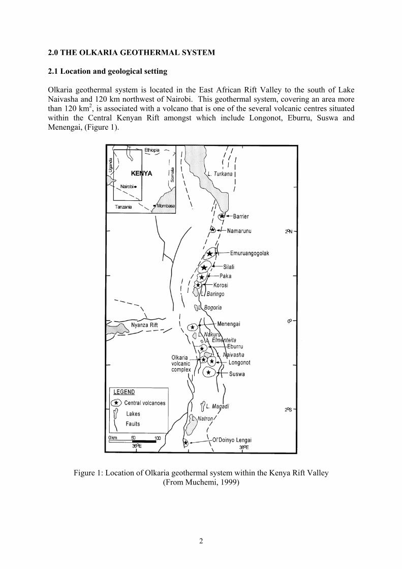
2.0 THE OLKARIA GEOTHERMAL SYSTEM 2.1 Location and geological setting Olkaria geothermal system is located in the East African Rift Valley to the south of Lake Naivasha and 120 km northwest of Nairobi. This geothermal system, covering an area more than 120 km2, is associated with a volcano that is one of the several volcanic centres situated within the Central Kenyan Rift amongst which include Longonot, Eburru, Suswa and Menengai, (Figure 1).
Figure 1: Location of Olkaria geothermal system within the Kenya Rift Valley (From Muchemi, 1999)
2

2.2 A brief history of the development Exploration of this geothermal resource was initiated by the United Nations and the Government of Kenya in 1956 and has been continuous since 1970. The early exploration work involved drilling of two wells OW-X1 and OW-X2 both of which are located in the northern part of the prospect (Figure 2). OW-X1 was drilled to 502 m and OW-X2 to 942 m. Although they encountered high temperatures, they failed to discharge and work was stopped in 1959 (KPC, 1981). In 1970, Olkaria Geothermal Project was initiated and was jointly financed by UNDP and the Kenya Government. During the same year, further exploration work consisting of geological mapping and geophysical and geochemical surveys as well as more investigations on the two exploration wells began. In 1972, well OW-X2 was coaxed into production through a small diameter pipe at atmospheric pressure and continuously produced for a year before being shut-in. Glover (1972) gave an estimation of the natural heat loss from the geothermal system to be close to 400 MWt with 90 % of this coming from steam discharge through surface vents. On the basis of the success in producing from well OW-X2 and the results of surface exploration, a technical review meeting was held in December 1972 and a recommendation made to drill four more exploration wells. Drilling started in 1973 with well OW-1 located to the southeast of the greater Olkaria system. This well was drilled to a depth of 1003 m and did not discharge on its own due to low temperature and permeability. The temperature measured at 1000 m was 126°C and the water rest level was 618 m below the wellhead. The well was stimulated into production by air-lift, but it could not sustain production. Following this unsuccessful result with well OW-1, it was decided to move about 3.5 km to the northeast of this well for drilling of well OW-2. Drilling of well OW-2 gave positive results. It was drilled to 1350 m and encountered a 240°C steam zone at 650 m. Maximum temperature recorded was 280°C at the bottom. Discharge at atmospheric pressure gave 70 – 75 % steam and total flow rate was 9 kg/s at a pressure of 6 bar-abs. It is due to the success in this well that further appraisal and production drilling were done in the vicinity culminating in the 1976 feasibility study for utilisation of geothermal steam for generation of electricity at Olkaria (SWECO and VIRKIR, 1976). The study indicated that development of the geothermal resource was attractive and the authorities decided to construct a 30 MWe power plant of two 15 MWe units with possible extension by addition of a third 15 MWe unit (Svanbjörnsson et. al., 1983). The first unit was brought on line in July 1981, the second in December 1982 and the third in April 1985. Since then, the geothermal field has been producing steam for generation of 45 MWe in the area currently called Olkaria East field. Further exploration drilling in the northeast and west of this field has led to demarcation of two more fields in which two more power stations are being constructed and each will produce 64 MWe. Generally, Olkaria geothermal system is now divided into East field, Northeast field, Central field, West field, Northwest field, Southeast field and Domes field (Figure 2). The total number of wells drilled to date is 102 and exploration drilling is now focussed in Olkaria Domes field and production drilling in Olkaria West field. Ormat Inc. is now developing Olkaria West field and they commissioned their first 13 MWe Binary cycle unit in August 2000. In this study, I will combine Olkaria East and Northeast fields and call it Olkaria East geothermal system, and will be my study area.
3

101
102
19
201202
204
26
27
28 2930
301
302
304
306
307 401
501
601
703 704
705706
707
708
709
710
711712
713
714715716
717718
719
721
723724
725726727
728
R2
203
308
3334
R3
5
801
901
902
903
25
32
720
305
1
701
M2
21
2320
8 910
312
1611
31 18
720
222 64 1315
12
X1
X2
193000 195000 197000 199000 201000 203000
Eastings (m)
9899000
9900000
9901000
9902000
9903000
9904000
9905000
9906000N
orth
ings
(m)
Olkaria West Field
Olkaria East Field
Olkaria Domes Field
Olkaria Northeast FieldOlkaria Central
Field
Olkaria Northwest Field
Olkaria Southeast Field
Study area
Figure 2: Location of the geothermal fields, drilled wells and the study area (the dots represent wells)
2.3 Geological overview Olkaria geology has been studied by many workers (Naylor, 1972; Clark et. al., 1990; Brown, 1984; Odongo, 1993; Muchemi, 1999; etc) and various views have been expressed but what seems to be a general consensus is that the geothermal field is a remnant of an old caldera complex which has subsequently been cut by N-S normal rifting faults that have provided loci for later eruptions of rhyolitic and pumice domes. Eruptions associated with Olkaria volcano and Ololbutot fault zone (Figure 3) produced rhyolitic and obsidian flows and then eruptions from Longonot and Suswa volcanoes (Figure 1) ejected pyroclastic ash that has blanketed much of the area. NW, NNW, N-S, NNE and NE trending faults and ring structure are observed in the geothermal complex (Muchemi, 1999; Odongo, 1993). The most prominent structures are the NE trending Olkaria fault, N-S trending Ololbutot fault, Olkaria fracture, the Ring fracture, Suswa fault and Gorge Farm fault. Subsurface stratigraphy of Olkaria wells shows that from the surface (which is at an average elevation of 2000 m a.s.l.) to about 1400 m a.s.l., the rocks consist of Quaternary comendites and pantellerites with an extensive cover of pyroclastics. Below these, the dominant rocks are trachytes with basalt flows and tuffs that mainly occur as thin intercalations (Figure 4). The rock stratigraphy is essentially horizontal (Muchemi, 1999; Brown, 1984).
4

Figure 3: Geological structural map of Olkaria geothermal system (from Muchemi, 1999)
2000
0
1000
OlolButotFaultOW-202 OW-201 OW-706 OW-720 OW-713
Superficials
Pyroclastics/Tuff
Rhyolite
Trachyte
Basalt
Elev
atio
n(m
.a.s
.l)
Olkariafault
Figure 4: General subsurface stratigraphy of Olkaria reservoir
5

Rocks down to 1400 m a.s.l. are nearly impermeable and act as caprock to the system. Below this depth permeability is encountered at the fractures, lava contacts and porous pyroclastic beds and tuffs. A look at well productivity indicates that wells located close to known or inferred faults produce highest mass flows hence indicating the importance of vertical permeability. Clay mineral analysis on cores and cuttings from wells OW-501 and OW-703 indicated the presence of smectite, carbonates and kaolinite. The presence of these minerals has been interpreted to indicate influx of cool low pH bicarbonate fluids into the reservoir from the north (Leach and Muchemi, 1987). Other hydrothermal minerals found in this field include zeolites, epidotes, pyrite, magnetite, haematite, calcite, quartz, adularia, chlorites, and illite. 2.4 Geophysical overview It is observed from resistivity measurements that low anomalies within the Olkaria geothermal system are controlled by linear structures in the NE-SW and NW-SE directions (Muchemi, 1999). The geothermal resource is defined by less than 15Ωm resistivity anomaly at 1000 m a.s.l. and occur at the intersection of these structures (Figure 5). High resistivity regions within or bounding these low resistivity anomalies coincide with NE and NW trending faults and are interpreted to be conduits channelling cold water recharging the system. It is inferred from MT data that deep low resistivity occurs at a depth of 4 - 5 km and is thought to define the heat source.
184000 186000 188000 190000 192000 194000 196000 198000 200000 202000 204000 206000 208000 210000
9892000
9894000
9896000
9898000
9900000
9902000
9904000
9906000
9908000
9910000
OW-026
OW-102
OW-201
OW-27
OW-30OW-301
OW-401
OW-501
OW-601
OW-704
OW-709
OW-714
OW-719
0W-801OW-001
OW-101
OW-304
OW-305
96001 96002
9600396003
96004
9600596006
96007
96008
96010
96012
96014
96015
96016
96018
9601996019
96021
9602296022
9602496024
9602596025
9602696026
9602796027
96028960289602896028
96029
96030
96031
96032
96033
9603496035
96036 96037
96038
96039
96040
96041
96042
9604496044
96045
96050
9605296053
96054
9605596055
96056
96057
96058
96059
96060
96061
96062
97001
97002
97003
97004 9700797007
97008
970099700997009
97011
97012970129701297013
97014
97015
B33
B40
B41
B42F1
F10
F11R
F2
F24F3
F5
F6
G2
G3
G4
G5
G7
GD01
LON59
LON69
Lon011
Lon018
M03
M10
M11M11R
M12
M13
M16R
M19 M2
M20
M21
M22
M23M24M24R
M28
M37
M38
M39
M4
M40
M41
M42
M43
M44
M45
M47
M5
M56
M57
M58
M6
M61
M62M64
M65
M7
M73
M75R
M76
M77
M78
M79
M7RM8
M81
M9
S11
S18
S19
S2
S3S3A
S5S5A
SL138
SL139
SL141
SL142
SL143
SL145
SL146
SL156
SL187
SL226SL230
SL231
SL233
SL234SL235
SL237
SL238
SL239SL242
SL245
SL247SL248
SL249
SL252
SL253
SL254
SL256
SL257
SL259
SL260
SL261
SL262
SL263
SL264
SL265
SL266
SL267
SL268
SL269
SL270
SL271 SL273
SL275
SL276
SL277
SL278
SL282
SL283
SL284
SL285
SL287
SL288
SL289
SL290
SL291
SL292
SL39
ST21
dl11
dl12
dl13
dl14d
dl15
dl16dl16
dl17
dl21dl21
dl23dl23
dl24dl24
dl25dl25dl25dl25
dl26dl26
dl27dl27
dl28dl28
dl31
dl32
dl33
dl34
dl35dl35
dl41
dl410dl410dl42dl43
dl44dl45d
dl49dl49
dl51 dl52 dl56dl56dl57dl57
dl71dl71
dom01dom02dom03
dom04
dom05
dom06 dom07
dom08
lk1
lk2
lk3
lk9
dom10
dom11dom12
dom13
dom14
0510152226303539404550556070100200
OLKARIA WEST
OLKARIANORTH-EAST
E.P.F.
DOMES
AKIRA
Figure 5: Integrated TEM and DC Schlumberger resistivity (Ωm) at 1000 m a.s.l. (source – Kenya Electricity Generating Company Ltd.)
6

Seismic monitoring of micro-earthquakes within the Olkaria geothermal system (Simiyu and Malin, 2000) has shown that shallow, high frequency events associated with movement of hot geothermal fluids, occur at the intersection of NE-SW and NW-SE trending faults. Deep, low frequency events, which have been associated with movement of cold water far from areas of strong heat source, occur away from these zones (Figure 6). Studies of shear wave attenuation beneath Olkaria geothermal field (Simiyu, 1998) indicate deep attenuating bodies below Olkaria hill, Gorge Farm volcanic centre and Domes area at about 7 to 18 km depth. These bodies coincide with zones of deep low resistivity and positive magnetic anomaly and have been interpreted to be zones of molten magmatic bodies that provide heat source for the Olkaria geothermal system. From magnetic studies, these bodies are approximated to be at temperatures above 575°C.
Figure 6: Location of micro-earthquakes in the Olkaria geothermal system (from Simiyu and Malin, 2000)
2.5 Geochemical overview The waters discharged by wells in the Olkaria geothermal system (before exploitation) vary depending on which field the well is located. Wells in Olkaria Northeast field discharge neutral sodium chloride waters with chloride concentrations in the range of 400 – 600 ppm and bicarbonate concentrations < 1000 ppm. Wells in Olkaria West field discharge mainly
7

sodium bicarbonate waters with concentrations about 10,000 ppm and chloride concentrations ranging from 50 – 200 ppm while wells in Olkaria Central field discharge a mixture of sodium chloride and sodium bicarbonate waters. Olkaria Domes wells discharge mixed sodium bicarbonate-chloride-sulphate waters with mean chloride concentrations of 180 – 270 ppm and Olkaria East wells discharge sodium chloride waters with chloride concentrations in the range of 200 – 350 ppm (Muchemi, 1999). Average temperatures calculated from silica geothermometer indicate 230 – 260°C for Olkaria East field, 265 – 270°C for Olkaria Northeast field, 186 – 259°C for Olkaria Central field and 232 – 242°C for Olkaria Domes field. K/Na ratio gives 230 – 260°C for Olkaria East field, 260 – 290°C for Olkaria Northeast field and 230 – 260°C for Olkaria West field. Calculated temperature declines towards northwest and east directions from areas around OW-701, OW-707, OW-726, OW-714, and OW-727 in Olkaria Northeast and to the south and southwest directions from areas around OW-305 and OW-301 in Olkaria West (Wambugu, 1996). The reservoir CO2 concentrations vary from > 10,000 ppm in Olkaria West field to < 10 ppm in Olkaria East field.
8

3.0 CONCEPTUAL RESERVOIR MODEL 3.1 Fluid and heat flow in hydrothermal systems The most basic features in a hydrothermal system are aquifers containing channels of hot fluid, paths for cold water recharge and heat source. Heat source, in most cases, is always intrusive magmatic bodies and cold water recharge originates as meteoric waters from ground surface and percolates down through faults and fissures to considerable depths where it is heated to high temperatures. The heated water rises through other faults and its place taken by incoming meteoric water. Heat is transferred from the heat source by conduction through the rocks and by convection due to fluid movements. In cold groundwater systems there is no variation in fluid density and flow is driven solely by pressure gradient between two points. The discharge is obtained according to Darcy’s law (Bear, 1979),
)( zg
Pdldgkq
w
+=ρµ
ρ (3.1)
However, in hydrothermal systems, due to buoyancy forces generated as a result of decrease in density when the cold meteoric water is heated at great depths, fluid flow may occur even against the direction of decreasing pressure gradient. A convective cell is formed between the upflow zone → cap rock outflow zone downflow zone → upflow zone. The flow characteristics within this cell are functions of Rayleigh number, Ra, given by (Kjaran and Eliasson, 1983):
→ →
λνβρ
w
ww TkhcgRa ∆= (3.2)
This gives the ratio of the buoyant forces to viscous resistance (in this case the viscosity of the of the fluid and the viscous drag of the rock matrix on fluids). For a horizontally fully saturated aquifer, convection will set in when Ra ≅ 4 (in geothermal reservoirs, Ra = 100 to 1000).
2π
This would imply that for convection to be maintained in a hydrothermal system, permeability has to be greater than some value for a given reservoir state. This condition can be expressed as:
Thcgk
ww
w
∆>
βρλνπ 24
(3.3)
We therefore see that, before exploitation, the initial fluid distribution in the hydrothermal reservoir is controlled by dynamic balance of mass and heat. Once exploitation begins, flow of fluid is controlled by the pressure gradient generated due to well discharge and flow to and from the wells will also be much greater than flow in the natural state. The part of a geothermal system exploitable for hot water and steam is no doubt related to its upflow zone. In this zone, especially in liquid dominated systems, due to the high pressures deep in the reservoir, water exists as liquid at some temperature. As the water rises due to 9

variations in density, its pressure falls and at some point when saturation pressure is reached, it will begin to boil and continue flowing up as steam and water mixture. Above the saturation point, temperature is obtained by the saturation relation:
)(PTT sat= (3.4) Below the saturation point temperature is nearly constant and pressure gradient is equal to the local hydrostatic gradient plus the dynamic gradient. The dynamic gradient, however, is very small and can be neglected and so the pressure relation is given by:
gdzdP
wρ= (3.5)
Equation 3.5 can be utilised to generate boiling point depth curve (BPD) for saturation conditions by solving numerically the following equation (Arason and Björnsson, 1994).
∫+=z
zsat dzgPzP
0
0)( ρ (3.6)
Discharge emanating from the upflow zone flows away laterally with almost no convection and can be treated in the same way as flow in cold groundwater. If the reservoir is liquid dominated and the wells exhibit hydrostatic pressure gradient, we can calculate fluid potentials in the flow domain and find the areal potential distribution. The result of doing this will be to show areas of high potential that will indicate hot upflow zones and areas of low potential that will indicate downflow zones for cooled water, leakage or discharge zones. The fluid potential at a point in the flow domain is defined as mechanical energy per unit mass and is given by:
gh=Φ (3.7)
where h is the hydraulic head given by
gPzhwρ
+= (3.8)
Since g is a constant, calculating hydraulic head is as good as calculating the fluid potential. 3.2 Temperature and pressures in the Olkaria geothermal system Formation temperature and initial pressures serve as the base for conceptual and numerical models and should be carefully analysed in order to get a good realistic model. Temperatures and pressures as measured from the wells are often affected by inter zonal flow within the wells, cooling of the formation during drilling, and cooling due to boiling during well discharge. Shallow cold groundwater may also leak through the casing annulus and cool the well. Temperature recovery after drilling can be estimated by Albright and Horner methods assuming that conduction is the major mode of heating. The resulting data can then be used to estimate the formation pressure (Arason and Björnsson, 1994). However, it is not possible to apply these methods when there is boiling in the well. In this case, it is necessary to check
10

the temperature and pressure logs for boiling conditions in comparison with boiling point for depth curve and the enthalpy of the discharged fluid. An attempt was made to estimate the formation temperature and pressures for all available wells in Olkaria. BOILCURV computer program for generating boiling point with depth curves and PREDYP program for calculating pressure in a static water column when the temperature is known (Arason and Björnsson, 1994) were used where appropriate. The estimated formation temperature and initial pressures are shown together with the measured data in Appendix A. This data was so much and its analysis took a very long time. It can be observed that temperature and pressures obtained from wells in Olkaria East field follow the boiling point with depth curve. Similarly, temperature and pressures from wells located in the upflow zones of Olkaria Northeast and West also follow the boiling point with depth curve. Wells outside these upflow zones show either isothermal temperatures at depth below the casing shoe, indicating inter zonal flow or reversed temperatures suggesting counter flow of hot outflow and cold inflow from shallow and deep aquifers, respectively. Areal temperature distributions (Figures 7 to 9) show hottest zones in Northeast field, West field and in the north around well OW-101. Coldest zones are in NE around well OW-704, in the NW around well OW-102, in the south and SW around wells OW-307 and well OW-801 and in the Olkaria Central field. Figures 10 and 11 show vertical cross-sections of temperature in the E-W and N-S directions. From the E-W section, we observe hot plumes in Olkaria West and Northeast fields separated by a cold temperature zone in Olkaria Central field. Some cooler down flow zone seem to occur within the hot plume in Olkaria Northeast. From the N-S section, we generally observe a wide zone of hot plume covering both Olkaria Northeast and Olkaria East fields with a cooler down flow zone between the two fields. Temperatures fall further south.
Figure 7: Temperature distribution at 1000 m a.s.l.
11

Figure 8: Temperature distribution at 500 m a.s.l.
Figure 9: Temperature distribution at 250 m a.s.l.
12

Figure 10: A general E-W temperature cross section
13

Figure 11: A general N-S temperature cross section
14

Figure 12 shows pressure distribution at 1000 m a.s.l. Low pressure zones are in the central and northwest corner and high pressure zones occur in the eastern and western sides. The low pressure zone in the central coincides with the low temperature and high resistivity zone and is also a zone of high steam loss from fumaroles. The high pressure zones coincide with upflow zones recharging the system.
Figure 12: Pressure distribution at 1000 m a.s.l. 3.3 Well Characteristics The casing design for the Olkaria wells consists of 20” diameter surface casing to a depth of 30 - 40 m, 13 3/8” diameter anchor casing to 260 – 350 m depth, 9 5/8” diameter production casing to 500 – 800 m depth and then 7” diameter slotted liners in the production hole (Figure 13).
26" Hole
17 1/2" Hole
12 1/4" Hole
8 1/2" Hole
20" dia.surface casing(30 - 40 m)
13 3/8" dia.anchor casing(260 - 350 m)
9 5/8" dia. productioncasing (500 - 800 m)
7" dia. slotted liner(1800 - 2500 m)
Most of the early wells drilled in the Olkaria East field intercepted low formation permeabilities in the range of 4 milli-darcy in the liquid zone and 7.5 milli-darcy in the steam zone (Bodvarsson and Pruess, 1984). Wells drilled later towards the north and generally in the Olkaria Northeast field have better permeabilities and are also better producers.
Figure 13: Casing design for Olkaria wells
15

Well productivity is affected both by inflow performance and wellbore performance. Inflow performance is the ability of the geothermal fluid to flow through the feed zone when there is a pressure drop between the reservoir and the well. It is greatly influenced by formation permeability. To a greater extent, Olkaria wells have low productivity because of the low permeabilities. Wellbore performance describes the contribution the casing design has on the pressure behaviour when fluid moves from the feed zone to the wellhead. It depends on the fluid temperature and reservoir pressure, well diameter and well depth. Since pressures and temperatures are unique properties of a particular reservoir, the only factor that can be optimised in wellbore performance is casing size. It has been shown for Svartsengi and the Geysers geothermal fields that increased casing sizes minimize wellbore effects leading to better well productivities (Kjaran and Eliasson, 1983). There is need to do studies on wellbore performance for Olkaria wells to investigate the effects and benefits of larger casing design. The data was not available to do this during this study. Figure 14 below is a N-S cross-section indicating location of feed zones in the wells. Most of the feed zones are intercepted at contact points between successive rock strata. Shallow feed zones in most of the wells produce steam.
0 1000 2000 3000 4000 5000 6000 7000 8000
Distance (m) from well OW-501
-1000
-500
0
500
1000
1500
2000
Elev
atio
n (m
.a.s
.l)
501
R2 708
712
727
720
728
713
R3
32 28 24 8 5 19 21 902
N S
Feedzone35 bar pressure contour
Figure 14: A N-S cross-section showing feed zones and 35 bar pressure contour
3.4 Pressure potentials and flow pattern in the Olkaria geothermal system Figures 15 – 17 show pressure potentials in the initial state in the Olkaria reservoir. High potentials occur in the western field and the eastern fields with a low potential between them. The low pressure potential extends to the south and indicates an area of rapid heat and mass sink (downflow or fluid and heat loss). High potential areas indicate zones of fluid and heat inflow/upflow. The arrows point to the possible direction of flow. Data analysis was done by using the formulas from section 3.1.
16

193000 195000 197000 199000 201000 203000
Eastings (m)
9899000
9900000
9901000
9902000
9903000
9904000
9905000
9906000
Nor
thin
gs (m
)101
102
19
201202
204
26
27
28 2930
301
302
304
306
307 401
501
601
703 704
705706
707
708
709
710
711712
713
714715716
717718
719
721
723724
725726727
R2
203
308
3334
R3
5
801
901
902
903
25
32
720
305
1
701
M2
21
23810
312
1611
31 18
720
22
Figure 15: Pressure potential (m) at 1000 m a.s.l. and flow directions
0 1000 2000 3000 4000 5000 6000 7000
Distance (m)
0
500
1000
1500
2000
Elev
atio
n (m
.a.s
.l)
OW
-301
OW
-302
OW
-202
OW
-203
OW
-201
OW
-711
OW
-706
OW
-712
OW
-727
OW
-715
OW
-707
OW
-714
OW
-716
OW
-704
Figure 16: A W-E cross-section of pressure potential
0 1000 2000 3000 4000 5000 6000 7000
Distance (m)
0
500
1000
1500
2000
Elev
atio
n (m
.a.s
.l)
OW
-501
OW
-708
OW
-727
OW
-701
OW
-728
OW
-713
OW
-R3
OW
-32
OW
-28
OW
-25
OW
-8O
W-5
OW
-21
OW
-902
Figure 17: A N-S cross-section of pressure potential
17

3.5 Conceptual reservoir model 3.5.1 Previous conceptual models Conceptual model of the Olkaria geothermal system has been reviewed several times over the years as more information is acquired from surface studies and deep drilling. The first model (Figure 18) was proposed by Sweco and Virkir (1976). In their model, the geothermal reservoir was visualised as boiling water overlain by a 50 – 150 m thick steam zone capped by tuffaceous caprock. Water originating from the surface penetrated down to 1600 m b.s.l. where on heating by heat flux from the underlying hot bedrock, it acquired a temperature of 320°C. This 320°C water then boiled off as it rises up to give a two-phase mixture of steam and water. The rising steam condensed below the cap rock and the condensate fell back ending in a convective circle.
Figure 18: 1976 conceptual model of Olkaria geothermal reservoir (from Sweco and Virkir, 1976)
In the model by Bodvarsson et al., (1987), fluid recharge to the Olkaria East reservoir was proposed to come from an upflow zone in the north close to OW-716. The steam zone (50 – 150 m thick) thinned towards the north and thickened to the south. The cap rock was proposed to be at 500 – 700 m depth. Another upflow zone was proposed to be in Olkaria West. The waters discharged from these areas were different with Olkaria West discharging
18

sodium bicarbonate waters and Olkaria Northeast and East discharging sodium chloride waters. Fluid discharged from the two upflow zones flowed along Olkaria fault from east and west to converge and flow to the south along Ololbutot fault with extensive steam loss along this fault. Part of the discharge from the Olkaria West upflow moved to the north along the Olkaria fracture. The latest review of the conceptual model is contained in Muchemi, (1999). The views expressed in the previous models have remained more or less the same and just refined and strengthened with additional information that has been acquired. Interpretation of MT and magnetic data together with surface geology has indicated that there is a highly differentiated magma chamber beneath the Olkaria geothermal system. Shallow heat sources occur along N-S, NW, NE striking faults and the ring fracture. Fluid movement is controlled by NW-SE and NE-SW faults and overall productivity of the fields and individual wells are correlated to the intersection of these faults, in the vicinity of the heat source. In addition to the two upflow zones proposed in the earlier models, a possible third upflow zone is proposed to be in the Olkaria Domes field. Fluid chemistry and reservoir temperatures seem to suggest that Olkaria West, Olkaria Central, Olkaria Northeast/Olkaria East and Olkaria Domes are in separate systems. 3.5.2 Revised conceptual model In this section, I now present a possible slight revision to the current conceptual reservoir model (Figure 19). The two distinct hydrothermal systems of Western and Eastern Olkaria are clearly separated by the low pressure potential and temperature zone of Olkaria Central. In the Eastern part, it seems possible that there are two upflow zones in Olkaria Northeast field and one upflow zone in Olkaria East field. A downflow zone extending from OW-723 through OW-R3/713 in a NE-SW direction seems to be separating Olkaria Northeast and Olkaria East fields. Olkaria East field is one big upflow zone that is possibly centred around OW-28, 30 and 32. From this zone, fluids move mainly to the south with extensive boiling occurring to develop steam zone below the cap rock. There is a possibility of a N-S fluid movement into the downflow zone. The two upflow zones in Olkaria Northeast are centred around wells OW-714, 716 and around wells OW-706, 720, 709, 728 and 701. A downflow zone extending from OW-717/718 through OW-708 in a NW-SE direction separates them. Extensive boiling also occurs in these two upflow zones to form steam caps below the cap rock. The other upflow zones occur around wells OW-301/305 area and well OW-101 area. OW-901 could be an extension of Olkaria East and from only three wells now drilled in Olkaria Domes, it is still not possible to delineate a separate upflow zone for this field. These observations are supported by distribution of high fluid potentials, high temperature distributions as well as shallow micro-earthquake clusters and low resistivity distribution around these zones. Calculated temperatures from geothermometers also point to support these observations. Cold water recharge into the reservoir seems to occur from all the directions. No clear marked hydrological boundaries can be observed from reservoir data or otherwise, in the Olkaria system. Olkaria Central seems to be a heat sink zone where there is tremendous cooling of the hot rising waters that come from the upflow zones. This cooling is evident from large steam discharge along Ololbutot fault and altered grounds in Olkaria Central field. Figure 19 gives a possible presentation of a conceptual model of the Eastern Olkaria system.
19

Elev
atio
n(m
.a.s
.l)
2000
1500
1000
500
0
-500
-1000
-1500
-2000
Groundwater flow Groundwater flow
340 °C
300 °C
240 °C
200 °C
OlkariaCentral
Gorge FarmFault orCaldera rim?
HEAT FLUX
Steam zone
Boiling water reservoir
0 6000 m
OW-201 OW-727 OW-714 OW-704OlolButotFault
Groundwater flow
Steam discharge
Upflow of hot boiling water
Downflow of cooled water
Figure 19: A revised conceptual model of the Eastern Olkaria system (section from east to west)
3.6 Hydrological model The regional groundwater flow in the Olkaria area is southwards from Lake Naivasha in the north (KPC, 1981). The Lake Naivasha catchments area includes the neighbouring escarpments of the Rift Valley. In the Eastern geothermal system, deep inflow of cooler recharge fluid into the reservoir seems to occur along the Gorge Farm fault in the northeast and along the fracture zone in Olkaria Central between Ololbutot fault and Olkaria hill. In the northern part, the regional groundwater flow seems likely to encroach into the geothermal system and mixes with hot water flowing from the upflow zone. This is supported by the occurrence of smectite, illite and chlorite-illite in the northern wells OW-501 and OW-703 and by their down hole temperature profiles and discharge behaviour. In general, the most likely hydrological setting are geothermal convective systems in three almost separate sections with segments of rapid downflow in-between them. Outflow through steam vents and compensating inflow are through active faults through the caprock.
20

4.0 LUMPED RESERVOIR MODEL In lumped-parameter (material and energy balance) models, the reservoir is considered as a single unit categorized by changes in a single set of variables. The model ignores any internal structure in the reservoir and the parameters to be determined are estimated from the averaged field history rather than from individual well information. The result of this is to match or forecast the gross behaviour of the reservoir. Normally, a lumped-parameter model only links the mass withdrawal to the changes in the production zone of the reservoir. It forecasts only the features of the production zone and if important processes occur outside this zone, the utility of the model is reduced (Grant et al., 1982). However, it is quite simple and offers a first step in evaluation of the collected data to indicate a rough direction of events. 4.1 Lumped convective model In this study, I will use a lumped convective model by Eliasson, 1973, and Kjaran and Eliasson, 1983, to estimate heat and mass flows in the upflow zones observed in the conceptual model. Darcy’s law for flow in the convective cell can be written as:
0. =∂∂
++∫ ∫ ∫ dsxpdsgUds
Kg ρ (4.1)
The first term is due to energy dissipation in the flow, the second due to buoyancy effects in the convection (density difference between the upflow and downflow) and the third term is due to the pressure gradient and must be equal to zero for the closed integration path. The first term can be approximated by:
luKgUds
Kg
ε−=∫ 1
(4.2)
where is the mass flux in the upflow andu ε is the energy dissipation factor and must be much smaller than 0.5. The second term is approximated by:
∫ ∆= ρρ glgds (4.3) where ρ∆ is the density difference between the downflow and upflow. Equating 4.2 and 4.3 and with A as the upflow area, the upflow can be estimated from the following equation:
ρε ∆−= )1(KAWup (4.4) The total natural heat loss is then obtained by:
)( downupwuploss TTCWH −= (4.5) This heat is lost through steam vents, surface springs and by conduction through the caprock.
21

Figure 20 below is a simple vertical lumped convective model of Olkaria Northeast field. It depicts hot water flowing up from the two perceived upflow zones in the conceptual model and out into the Olkaria Central area and well OW-704 area. Cooled water enters the convective cells at depths beneath these outflow areas. In the middle of the two convective systems, there is some mixing of fluids from the two upflow zones with steam condensate and possibly shallow groundwater leaking through the cap rock. Steam leakages through the faults occur at the surface and cold meteoric water also flows down through the faults. If the upflow areas are estimated as the extent of 1800 m pressure potential at 1000 m a.s.l. (Figures 15 and 16), then the upflow rates can be estimated as flows:
Upflow of132 kg/s of appr. 300 °Cwater
Upflow of 218 kg/s ofappr. 300 °C water
Downflow of 180 °Cwater
Downflow ofappr. 160 °Cwater
1 2
23.7 kg/s of steam
46 kg/s of steam
Cold waterinflow ? Cold water
inflow ?
Figure 20: A convective model of Olkaria Northeast reservoir Average transmissivity obtained from interference tests done in Olkaria Northeast field (Ofwona, 2000) is 20 darcy-meter and transmissivity in the Olkaria fault as estimated from numerical model (Bodvarsson, 1993) is 200 darcy-meter. Assuming a reservoir thickness of 1000 m, average permeability is obtained to be 18 milli-darcy. If we assume that the upflow water is 300°C, then the hydraulic conductivity is calculated as K = (18 x 10-15 m2 x 9.81 m/s2)/0.127 x 10-6 m2/s = 1.4 x 10⁻⁶ m/s. For cell 1, ρ∆ = 900 – 712 = 188 kg/m3, A = 1 x 10⁶ m2 and for cell 2 ρ∆ = 920 – 712 = 208 kg/m3, A = 1.5 x 10⁶ m2. Using Equation 4.4, upflow rate in cell 1 = 132 kg/s and in cell 2 = 218.4 kg/s. Heat flow from cell 1 is then 132 kg/s x 4.2 kJ/kg°C x 120°C = 66.5 MWt and from cell 2 equals to 128.4 MWt. If this is solely lost by steam vents to the surface, amount of steam expelled will be equal to about 70 kg/s. 4.2 Lumped exploitation model An overall material balance for a producing geothermal reservoir is given by the expression
ripon MMMMM ++−= (4.6) It states that the mass of fluids in the reservoir now equals to what was originally in place, less what has been produced, plus what has been injected and what has recharged the reservoir from the external source. A fall in reservoir pressure can be measured and related to the mass of fluid produced.
22

The conservation of mass equation for a basic reservoir model with discharge and recharge, with fluid withdrawal from the reservoir and reservoir recharge from an external source, can be written as (Grant et. al., 1982):
0=−+ rm WW
dtdPS (4.7)
If the reservoir contains boiling water overlain by a steam or vapour dominated zone, like the case of Olkaria East field, then because of the high compressibility of the vapour zone, pressure in this zone may be considered constant. Analysis of drawdown data can be treated as in unconfined reservoir case with fluid withdrawal assumed to be mainly from the water zone with the upper compressible region remaining undisturbed. Pressure in the liquid zone can be assumed to be in hydrostatic equilibrium. If the reservoir pressure falls by an amount
P∆ , a fall in water level of an amount gP wρ/∆ results. Total volume loss is given as,
gPAV
wρφ∆
=∆ (4.8)
and
φρA
gqdtdP w= (4.9)
giving
gASmφ
= (4.10)
The recharge rate is approximated by:
PW rr ∆= α (4.11) Here rα is lumped recharge coefficient that incorporates the effects of permeability and thickness of the matrix through which recharging fluid traverses. Equation 4.7 can then be written as:
dtdPSPW mr −∆=α (4.12)
Solution to this equation for a constant production rate starting at time t = 0 is given by:
( ξ
α/1 t
r
eWP −−=∆ ) (4.13)
where
r
mSα
ξ = (4.14)
23

is the response time constant for the system. For short times (t << ξ ), recharge is negligible and pressure will decline almost linearly with time:
mSWtP =∆ (4.15)
At steady state, i.e. large discharge times much greater than the time constant (t >>ξ ), the pressure will stabilise at a value determined by a balance with the recharge:
r
WPα
=∆ (4.16)
For variable discharge rates, we define a unit response function for the reservoir as:
∫ −=∆t
dtfWP0
)()( τττ (4.17)
where f is the instantaneous unit response function for the reservoir. Another response function can be defined as:
∫=t
dfF0
)()( τττ (4.18)
which in this case is given by:
)1(1)( /ξ
ατ t
r
eF −−= (4.19)
The solution for variable discharge rate is then given by:
)()()( 11 −− −−=∆ ∑ iii
i ttFWWtP (4.20)
As we have seen above, for an unconfined liquid dominated reservoir, production of fluid will result in a fall in reservoir liquid level. The original liquid in place is given by
φρAhM o = (4.21) and drawdown equation without recharge or water influx can be expressed from Equation 4.8 by:
φρAM
h p=∆ (4.22)
This implies that a graph of drawdown (whether water level or pressure) with cumulative mass production should be a straight line if there is no water influx. These ideas are applied in chapter 6.
24

5.0 NUMERICAL MODEL 5.1 Theoretical background 5.1.1 General partial differential equations for flow in two-phase geothermal reservoirs In geothermal reservoirs, mass is carried through the medium by the percolation of fluid through the system of pores and fractures while heat is transferred by convection, conduction (diffusion) and dispersion. The process of heat transfer alters the density of the fluid, thus creating buoyancy forces that alter the course of the flow. Flow without heat transfer is a linear process and all velocities and fluid pressures are determinable from the boundary values. No streamlines are created within the fluid and the flow is entirely dependent on the external pressure conditions. Flow with heat transfer is a non-linear process depending both on pressure and temperature at the boundary. Streamlines may be created within the fluid and if there is no flow through the boundaries, internal flow can occur. Due to the non-linearity of these processes, the equations describing flow in geothermal systems can only be solved by numerical methods since no analytical solutions exist. The partial differential equations governing two-phase flow of water and steam in geothermal systems can be written for conservation of mass, momentum and energy with the necessary constitutive relationships and equation of state. Assuming a homogeneous isotropic media and neglecting solute transport, chemical reactions, kinetic energy, viscous dissipation and potential, these equations take the following forms: Conservation of mass For a rock matrix saturated with steam and water mixture, a fraction of the pore space is filled with each phase. The fraction of pore space filled with water is Sw and the remainder, 1- Sw, is occupied by steam. A unit reservoir volume then contains in its pore space a mass wwS ρφ of water and a mass swS ρφ )1( − of steam, giving a total fluid mass per unit volume of wwS ρφ +
swS ρφ )1( − . Both liquid and vapour phases can move independently through the medium and hence there are separate mass flux densities for the individual phases. The conservation of mass equation for the case where there is a source (or sink) term is therefore written as:
( ) Msswwwsww QqqdivSSt
=++−+∂∂ )()1( ρρφρφρ (5.1)
Conservation of energy The total energy contained in a unit volume of the reservoir is the sum of energy contained in the rock, rrUρφ )1( − , and that contained in the two-phase fluid, www US ρφ + ssw US ρφ )1( − . Energy is transported through the reservoir by convection and conduction. The convective flux is given by sssw hqhwwq ρρ + and the conductive-dispersive flux by T∇λ . The equation for conservation of energy can therefore be written as (White and Kissling, 1992):
( ) Essswwwrrswswww QThqhqdivUUSUSt
=∇−++−+−+∂∂ )()1()1( λρρρφφρφρ (5.2)
25

Conservation of momentum When two phases occupy the same pore volume, each reduces the flow of the other below what it would be if it fully saturated the medium. The resulting permeability reduction factors are called relative permeabilities and are functions of water saturation. For two-phase flow of steam and water, Darcy’s law takes the form:
)( gPk
kq ww
rww ρ
µ−∇−= (5.3)
)( gPk
kq ss
rss ρ
µ−∇−= (5.4)
Constitutive relations A single-phase reservoir contains at any time a distribution of pressure and temperature and a two-phase reservoir contains pressure-temperature and saturation. These primary thermodynamic variables must be supplemented with constitutive equations that express secondary variables and parameters as functions of a set of the primary variables of interest. The existence of steam and water in contact means that the pressure and temperature are related by the saturation curve and due to capillarity effects, the vapour pressure of the water phase will be lowered. The constitutive relations therefore, are: P = Psat(T) or T = Tsat(P) (5.5) Pcap (Sw) = P - Pw (5.6) Various empirical functions of relative permeabilities and capillary pressures are available from various authors and are documented Grant et al., 1982; Kjaran and Eliasson, 1983; and Pruess et al., 1999; among others. The coupling of pressure and temperature through the saturation relation means that the mass and energy conservation equations are strongly coupled (Grant et. al., 1982) making the thermodynamic properties (density, viscosity, enthalpy and internal energy) be functions of a single variable (pressure or temperature) hence simplifying the task of solving the equations. The solutions to these equations are obtained numerically by use of either finite difference or finite elements method. The former is the widely used method by geothermal modellers. 5.1.2 Finite difference formulations Aquifer discretization is done in both space and time. The region of interest is divided into blocks or volume elements (Figure 21) using the Cartesian coordinate system. The aquifer and fluid properties are assumed to be constant throughout the element, but are allowed to differ between different elements. In this way, a non-homogeneous aquifer is approximated as a collection of different homogeneous regions. Elements are node centred and boundaries separating the elements are located at an equal distance from each node. The discretized flux is expressed in terms of averages over parameters for elements i and j.
26

Element i Element j
AijAij
Dij
Fmij
Element i Element j
Figure 21: Volume elements
Time is discretized as a first order finite difference and the flux and mass/energy accumulation terms are evaluated at the new time level; to obtain the numerical stability needed for an efficient calculation of multiphase flow (Pruess et. al., 1999). In this way, the fluxes are expressed in terms of the unknown thermodynamic parameters at the time step , so that these unknowns are only implicitly defined in the resulting equations. Time discretization of equations 5.1 and 5.2 results in the following set of coupled non-linear algebraic equations (Yang et. al., 1991):
ttt nn ∆+=+1
1+nt
Mass balance ( ) ( ) 01
11
11 =∆−∆+− ++
+++ ∑ n
nmin
j
nmijij
nmi
nmii tQtFAMMV (5.7)
Energy balance ( ) ( ) 01
11
11 =∆−∆+− ++
+++ ∑ n
nein
j
neijij
nei
neii tQtFAMMV (5.8)
where,
( 11 )1( ++ −+= niwswwi
nmi SSM ρρφ ) (5.9)
( ) 111 )1()1( +++ −+−+= n
iririniswswwwi
nei TCUSUSM ρφρρφ (5.10)
and Ur = Cr T (5.11) The mass flux consists of both liquid (water) and vapour (steam) phases and can be written as:
1+nmijF = + (5.12) 1+n
mijwF 1+nmijsF
and in terms of Darcy’s law as:
−
−
−= +
+++
+ij
nwij
ij
ni
nj
n
ijw
rww
nmijw g
DPPkk
F 1111
1 ρµ
ρ (5.13)
27

−
−
−= +
+++
+ij
nsij
ij
ni
nj
n
ijs
rss
nmijs g
DPPkk
F 1111
1 ρµ
ρ (5.14)
The energy flux is written as:
ij
ni
njn
ijn
mijsnsij
nmijw
nwij
neij D
TTFhFhF
11111111
++++++++ −
−+= λ (5.15)
The weighted interface densities are linear averages and are written as:
)(21 11 ++ += n
wjnwiwij ρρρ (5.16)
)(21 11 ++ += n
sjnsisij ρρρ (5.17)
Permeability is harmonically averaged and is obtained from:
+=
j
j
i
i
ij
ij
kd
kd
kD
(5.18)
Interface mobility and enthalpies are evaluated from (Yang et. al., 1991):
1+
n
ijw
rww
kµ
ρ = 1+
n
iw
rww
kµ
ρ (5.19)
and (5.20) 11 ++ = n
winwij hh
for
0111
<−−
+
++
ijn
ij
nn
gD
PPwij
ij ρ (5.21)
1+
n
ijs
rss
kµ
ρ = 1+
n
is
rss
kµ
ρ (5.22)
and
11 ++ = nsi
nsij hh (5.23)
for
28

0111
<−−
+
++
ijn
ij
nn
gD
PPsij
ij ρ (5.24)
11 ++ = n
wjnwij hh (5.25)
for
0111
>−−
+
++
ijn
ij
nn
gD
PPwij
ij ρ (5.26)
11 ++ = n
sjnsij hh (5.27)
for
0111
>−−
+
++
ijn
ij
nn
gD
PPsij
ij ρ (5.28)
5.1.3 Solutions to the discretized equations Equation 5.7 and 5.8 can be written in residual forms as:
( ) ( ) 011
111
12 =∆−∆+−= ++
+++
− ∑ nnmin
j
nmijij
nmi
nmiii tQtFAMMVR (5.29)
( ) ( ) 01
11
112 =∆−∆+−= +
++
++ ∑ nnein
j
neijij
nei
neiii tQtFAMMVR (5.30)
These equations are applied for each volume (block) element Vi, for all the blocks in the reservoir. The unknowns are the independent primary variables, pressure and temperature (or saturation) in the ith block at the end of (n + 1)th time step (that is, , (or )). The secondary parameters
1+niP 1+n
iT 1+niS
wρ , sρ , , , wU sU wµ , and sµ are calculated from the primary variables by use of Steam Table data. Equations 5.29 and 5.30 can be solved by Newton’s iteration method (Appendix D) or more rigorous and fast converging iterative methods such as conjugate gradient, pre-conditioned conjugate gradient, Bi-Conjugate Gradient Stabilized etc (Moridis and Karsten, 1998;). To obtain the approximate solutions, the residuals are minimized or reduced to a preset convergence tolerance after a number of iterations otherwise the time step is reduced and a new iteration is started. Because of the large number of numerical computations involved, computer softwares have been developed to solve these equations. TOUGH is one of the widely used for geothermal applications and has been used for modelling Olkaria reservoir before. It will therefore form the basis of my numerical modelling study. TOUGH (acronym for Transport Of Unsaturated Groundwater and Heat) was developed at Lawrence Berkeley Laboratory. It is a general-purpose software which can handle a wide variety of flow problems in the field of geothermal reservoir engineering, nuclear waste
29

isolation, environmental assessment and remediation, and unsaturated and saturated zone hydrology. It is a commercially available software and the details of its architecture is documented in Pruess et al., (1999). 5.2 Previous numerical simulation work in Olkaria Several numerical simulation studies have been carried out in Olkaria from 1980 to 1993. These include Bodvarsson, 1980; Bodvarsson and Pruess, 1981; Bodvarsson et al., 1982; Bodvarsson et al., 1987, Bodvarsson and Pruess, 1987 and Bodvarsson, 1993. In the 1980 study, a simple vertical model was employed to study the effects of vertical permeability on the production capacity. The objective was to evaluate if fluid production should be limited to the steam zone or if the long-term reservoir performance would improve with combined production from both steam zone and underlying boiling reservoir. The main conclusion was that excessive production from the steam zone would cause localized boiling and pressure decline, thus limiting the productive life of the system and production from the underlying liquid dominated zone would lead to a counter flow of steam and liquid, resulting in optimal depletion of the reservoir. The 1981 studies dealt with the effects of horizontal and vertical permeability and the importance of areal extent of the production area. The simulation neglected the steam zone and considered only a 550 m thick water dominated zone. The results showed that a long-term production of 45 MWe was possible at Olkaria. In the 1984 work (Bodvarsson et. al., 1987), a detailed three-dimensional well by well model was developed for the Olkaria East field using the numerical code MULKOM. The model was calibrated against 6.5 years of production history and investigated various reservoir development schemes to study the effects of different well spacing on well deliverabilities, power production of 45 MWe and 105 MWe and the effects of injection on well performance and reservoir depletion. The results showed that an optimum density of 11 wells per square kilometre was the most suitable and that an area of 2 km2 was appropriate for production of 45 MWe for 30 years but 9.5 km2 would be required for production of 105 MWe. It also showed that injection would help in sustaining steam flow rates from wells. In the 1987 model (Bodvarsson and Pruess, 1987), a detailed 3-Dimensional natural state model of the entire Olkaria geothermal field was developed. The results indicated that two major upflow zones, in Olkaria Northeast and West feed the geothermal system at a total recharge rate of 600 kg/s with the one in Olkaria West being 350 kg/s and the one in Northeast being 250 kg/s. The fluids from the two upflow zones mix near well OW-201 and discharge mostly southwards along the Ololbutot fault (260.5 kg/s) with a smaller discharge to the north along the Olkaria fracture zone (175.1 kg/s). Heat amounting to 400 MWt is lost from the system with most of it through steam fumaroles. The Olkaria East wells are fed by about 50 kg/s from the Northeast upflow zone and the average permeabilities of the major faults and fractures were estimated to be hundreds of milli-darcies. In the 1993 model (Bodvarsson, 1993), the aim was to investigate the generating capacity of Olkaria Northeast geothermal reservoir, effects of reinjection both on individual wells and the entire reservoir performance and the degree of interference that might occur between the Olkaria Northeast and East reservoirs. The model was run in TOUGH and the results concluded that the Northeast reservoir was capable of 64 MWe and probably more power production for 30 years and that due to its relatively high permeabilities and temperatures compared to the East field, it would have modest pressure and flow rate declines, especially if
30

reinjection is employed. Interference between the East and Northeast reservoirs would also be minimal. 5.3 Present work Between the year 1987 and 2000, 9 wells have been drilled and are producing in the East field, 5 wells drilled and tested in the West field, 3 in Central field, 1 in Southeast field, 25 in Northeast field and 3 in the Domes field. Most of the new wells drilled in the Northeast field were included in the model by Bodvarsson (1993). In the present work, just for study purposes, I will make use of the existing 3-D natural state numerical grid developed by Bodvarsson and Pruess (1987), and attempt to recalibrate it with the data from all the new wells that were not drilled by then. I will then try to match the production history data with the updated model. 5.3.1 An update to the existing 3-D natural state model of the entire Olkaria system The objectives of natural state modelling is to help in validating the conceptual model and to quantify the natural mass and heat flow within the hydrothermal system as well as to provide the initial thermodynamic conditions for exploitation modelling. It involves setting up of a model with an approximate permeability structure based on the conceptual model. A numerical grid of the system is used during the computer simulation runs to match the observed (or measured) thermodynamic field conditions such as temperature and pressure distributions. The simulation of the model should be carried out over a long period of time approximating to the development of the geothermal system over geologic time. Iterations are performed by adjusting parameters such as permeability distribution, mass and heat flow into and out of the system and boundary conditions on lateral as well as top and bottom boundaries until the calculated results match the observed data. Figure 22 shows the grid used by Bodvarsson and Pruess (1987), to model 3-D natural state of the entire Olkaria geothermal system and which is also used in this work. It covers an area of 110 km2 and is partitioned into 128 blocks. In the vertical dimension, the model assumes an impermeable caprock of 700 m thickness beneath which underlies a permeable reservoir of 850 m total thickness that is further partitioned into three layers so as to give a total of 384 grid blocks. When this model was developed, the existing wells drilled by then were between 900 m to 1600 m depth (1100 m a.s.l. to 400 m a.s.l.) and so this covered them pretty well. However, wells drilled later on have been deeper and have intercepted deeper aquifers. Initial and Boundary conditions In order to obtain a solution to the governing equations, hydrodynamic and thermal boundary conditions must be specified. These conditions can be deduced from a thorough examination of hydrologic and thermodynamic data and from data obtained by geologic, geophysical and geochemical investigations. The major hydrogeologic features of the Olkaria system include Olkaria fracture, Olkaria fault, Suswa fault, Gorge farm fault and Ololbutot fault (Figure 3). In the model of Bodvarsson and Pruess (1987), the hydrothermal system is recharged by two major upflow zones located near the western and eastern ends of the Olkaria fault. The fluid from the upflow zones move along the Olkaria fault as they undergo conductive cooling as well as cooling by steam loss to the surface and converge in Olkaria Central zone. Major outflow with substantial steam loss and cooling occurs towards the south along the Ololbutot fault and
31

towards the north along Olkaria fracture zone. The reservoir is assumed to be bounded in the east and west by no flow boundaries (very low permeability) and in the north and south by constant pressure boundaries of 45 bars at 1075 m a.s.l. and 28 bars at 1075 m a.s.l., respectively. The main model parameters are summarized in Table 1.
191 192 193 194 195 196 197 198 199 200 201 202 203 204
Eastings (km)
9896
9897
9898
9899
9900
9901
9902
9903
9904
9905
9906
9907
Nor
thin
gs (k
m)
151
2
3
4
7
1377
5
A2 A3 A4 1A5 2A5 1A6 A7 A8 A9 A10 A11
1B1B2 B3 B4 1B5 2B5 1B6
B7B10 B11
1C12C0 2C1
1C2
21C3
2C31C4
1C5
2C5 1C6 C7 C10 C11
D1 1,D2 1,D32,D3
1,D42,D4
1,D5 2,D5D5 D5
1,D6
2,D6D7D7
1,D8 1,D9 D10
DE0 E1E2 1,E32,E3 E4
1,E5 2,E5 1,E61,E7 E8
E81,E92,E9
1,E10
2,E10
F1 F2 1F32F3
F4 1F5 2F5 1F6 F7 F8
FG0
G1 G2 1G32G3 G4 1G5 2G5 1G6 G7 G8
H23 H4 1H5 2H5 1H6 H7 H8 H9
HI10
I3 I4 1I5 5 1I6 I7 I8 I9
J4 1J5 2J5
1J62J6
J7 J8 J9
1K5 2K5 1K61K7
2K7
1K82K8 K9
JK10
2000
1300
1200
950
450
Caprock
Layer 1
Layer 2
Layer 3
Vertical section
Elev
atio
n (m
.a.s
.l)
Olkaria FractureA
E
B
CD
Olkaria Fault
Ololbutot Fault
Suswa Fault
Gorge FarmFault
X1
1
5810
11
8
212223
2526
2728 9
30
31
3234
101102
201202203
204
301
02
304
305
306
307
308
401
501
601701
703 70
705
707
708710
11
7
716
1820
721
72727
801
901
902
903
R2
R3
B8 B9
2CC8
C9
3, 4,1,2,
2,1,
F9
2I
Figure 22: Grid used in the current 3-D numerical model
Model update Appendix B1 shows graphs detailing pressures and temperatures calculated by the recalibrated model (this work) and those from the 1987 model in relation to the estimated formation temperatures. We can observe that the 1987 model matches the data pretty well except for the wells within the low temperature zone in Olkaria Central field. To obtain a reasonable match for these wells, I reduced the upflow rate from the west and permeability in the Olkaria fault and Olkaria fracture zones and increased the permeability of the East field thus allowing more fluid to divert south through the present production field instead of moving to the Central field. Other minor adjustments in permeabilities on other elements were also necessary. Table 2 gives a summary of the main adjustments done to recalibrate the old model. 5.3.2 Production history matching After performing a successful natural state simulation that matches relatively well the observed thermodynamic conditions, the model is now used as an initial state for the exploitation modelling. The main objective here is to have a model that will be able to simulate the observed data. The data to be matched are usually the production rate history and enthalpies as well as pressure drawdown. Parameters that are adjusted include porosities, permeabilities and flow rates (production indices). Other rock properties are assumed constant.
32

From the reservoir data, it is observed that the fluid in-place in Olkaria East field is a mixture of liquid water and steam. We therefore have to employ Darcy’s equation for two-phase flow as discussed earlier. This implies that relative permeabilities have to be introduced. In the previous simulation by Bodvarsson and Pruess (1984), relative permeabilities were assumed to be linear functions of saturation as indicated in Table 1 and the same will be employed in this work. Wells in Olkaria have multiple feed points. The best way to model this would be to allow fluid to flow into the well by assigning a productivity index and fluid mobility and pressure in the feed zone. There are very few data regarding productivity indices of Olkaria wells so to do this would require parameter adjustment during simulation. Due to limited time available, this could not be done for this study. The production rates from different layers were therefore specified and varied in different proportions of the total rate so as to be capable of maintaining reasonable enthalpies and pressures (forced flow). In this work, production was assumed to come from one well each located in block A8, B7, B8, B9, and C9 (Figure 22) and each producing out of 3 feed zones, one in each model layer. Injection history described in the next chapter was also implemented. Percentage of flow rates extracted from layers in the producing blocks are shown in Table 3. Best model Appendix B2 has the graphs of production history matching. The graphs give relatively good match to production data. Cases where there exists a drastic decline in enthalpy as in element B8 could not be avoided due to the fact that cold water is injected into the same element that is being produced from. However, the low enthalpies calculated due to injection still agree quite well with the measured in the wells that were affected by cold injection such as well OW-16 and OW-19 (Appendix C). The high extreme in the enthalpy happening in 1985 to 1986 is due to over production that occurred when turbine number 3 was added to the system. Thereafter, a drastic decline in reservoir pressure followed as the reservoir was adjusting to the high load. The high extreme starting in 1998 is due to connection of the deepened well OW-5 which now produces from deeper aquifers that are not included in the grid. Pressures obtained also agree quite well with the measured data (Chapter 6 and Appendix A). For example the calculated pressure data for elements B7 and B8 (where most production has taken place) are quite comparable with the measured data. The calculated pressure in layer 3 of element B 8 is 58 bars in July 2000 and is equal to with the measured pressure at 1300 m in well OW-8 in October 2001 (58 bars).
33

6.0 OLKARIA EAST FIELD RESPONSE TO PRODUCTION 6.1 Production history Olkaria East geothermal field has been under commercial exploitation since July 1981 when the first 15 MWe generation unit was commissioned. Additional two 15 MWe units were put on line in December 1982 and April 1985. Since then the field has been generating 45 MWe of electricity. Initially, 23 wells (OW-2, 4, 5, 6, 7, 8, 10, 11, 12, 13, 14, 15, 16, 17, 18, 19, 20, 21, 22, 23, 24, 25, and 26) supplied steam for the three units but as time progressed, some wells declined in output and had to be isolated. New make-up wells were drilled to restore the generating capacity, which had declined to 31 MWe by 1994 (Mwangi, 2000). Four make-up wells (OW-27, 28, 29 and 30) were connected in 1995 and two more (31 and 33) in 1996. Figure 23 shows the field production history, the values of mass rates are yearly averages and the enthalpies are weighted averages. Mass production during well testing has been neglected.
1981
1982
1983
1984
1985
1986
1987
1988
1989
1990
1991
1992
1993
1994
1995
1996
1997
1998
1999
2000
Year
0
50
100
150
200
250
300
Flow
rate
(kg/
s)
0
500
1000
1500
2000
2500
Enth
alpy
(kJ/
kg)
WaterSteamTotal massEnthalpy
Figure 23: Production history 6.2 Re-injection/Injection history Well OW-3 A tracer and injection test experiment was done in well OW-3 from April to September 1993 (Ambusso, 1994). Cold fresh water at 18°C from Lake Naivasha was injected in this well continuously for 172 days at an average rate of 100 t/hr (27.78 kg/s). 125 kg of Sodium
34

fluorescein dye was introduced as a slug after 45 days of injection. Production and chemical changes were observed in wells OW-2, 4, 7, 8, 10 and 11. Chloride decline occurred in wells OW-2 and 4 during the injection period and tracer returns were observed in wells OW-4, 2 and 7 with OW-4 registering the highest recovered mass of about 38 %, well OW-2, 0.1 % and well OW-7, 0.07 % (Ofwona, 1996). Hot re-injection of separated brine from wells OW-27, 31 and 33 has been going on in this well (OW-3) since May 1995 at approximately 13 t/hr (3.6 kg/s). Well OW-12 Tracer/injection test experiment was done in this well from 12.7.96 to 1.9.97. Cold fresh water from Lake Naivasha was injected continuously at an average rate of 100 t/hr (27.78 kg/s) for 416 days. 500 kg of Sodium fluorescein tracer was introduced as a slug after 20 days of injection. Wells around OW-12 were monitored for chemical and output changes. High tracer returns were obtained from wells OW-15, OW-16 and OW-19. The same wells also experienced drastic decline in chloride concentration and enthalpies with big increase in water flow. Well OW-R3 Tracer/injection test experiment was done in this well from May 1995 to July 1.9.96. Cold fresh water from Lake Naivasha was injected continuously at an average rate of 100 t/hr (27.78 kg/s) over the duration of the experiment. 500 kg of Sodium fluorescein tracer was introduced as a slug after 27 days of injection. Wells close to OW-R3 were monitored for chemical and output changes. Very little tracer returns were obtained from wells OW-25, OW-29 and OW-30 and none from the closest wells OW-32 and 34. There was also very little or no change at all in the fluid chemistry as well as production output from the neighbouring wells. Other tracer and injection experiments have been done in wells OW-R2 and OW-704 (Karingithi, 1995) in Olkaria Northeast field. 6.3 Changes due to exploitation Appendix C shows production history of some selected wells in the producing field and Figures 24 to 27 show changes in reservoir chloride and enthalpies. The field response can be summarized as increased boiling in the centrally located wells giving rise to dry steam and high chloride concentration and induced recharge in the wells located at the periphery resulting in modest decline in chloride concentration and enthalpies. The recharging of these wells is also supported by the slow pressure depletion rates depicted in their downhole data (Figure 21 and Appendix A). 6.4 Pressure drawdown Due to high demand of steam, no wells within the production field were available specifically for monitoring pressure response due to production. Only well OW-3 and well OW-9 were considered unsuitable for production and could have been used for this purpose but well OW-3 was used for field injection experiments and well OW-9 had internal flow and was also later on plugged due to its close proximity to the project offices. However, well OW-8 offered some good pressure decline history. This well was first drilled to 1080 m in November 1978 and intercepted permeable zones at 600 - 700 m and 900 - 1080 m depth. It was then
35

deepened to 1600 m in 1983 intercepting more permeable zones at 1300 – 1400 m. It remained shut-in from 1979 to 1983 and again to September 1985 when it was connected to the steam supply system. Production from this well continued until October 2000 when it was shut-in. Pressure and temperature measurements were done in October 2001 and the pressure data can be seen in Figure 28.
199.4 199.8 200.2 200.6 201.0
Eastings (km)
9901.0
9901.2
9901.4
9901.6
9901.8
9902.0
9902.2
9902.4
Nor
thin
gs (k
m)
OW-2
OW-3
OW-4OW-5
OW-6
OW-7
OW-8OW-9
OW-10
OW-11
OW-12
OW-13
OW-14
OW-15
OW-16
OW-17
OW-18
OW-19
OW-20
OW-21
OW-22
OW-23
OW-24OW-25
OW-26
OW-27
OW-28 OW-29
OW-30
OW-31
OW-32
OW-33
OW-34
200
300
400
500
600
700
800
900
Chloride conc. (ppm)
Figure 24: Chloride concentrations in 1986
Enthalpy (kJ/kg)
1800
1900
2000
2100
2200
2300
2400
2500
2600
2700
199.4 199.8 200.2 200.6 201.0
Eastings (km)
9901.0
9901.2
9901.4
9901.6
9901.8
9902.0
9902.2
9902.4
Nor
thin
gs (k
m)
OW-2
OW-3
OW-4OW-5
OW-6
OW-7
OW-8OW-9
OW-10
OW-11
OW-12
OW-13
OW-14
OW-15
OW-16
OW-17
OW-18
OW-19
OW-20
OW-21
OW-22
OW-23
OW-24OW-25
OW-26
OW-27
OW-28 OW-29
OW-30
OW-31
OW-32
OW-33
OW-34
Figure 25: Enthalpies in 1986
199.4 199.6 199.8 200.0 200.2 200.4 200.6 200.8 201.0
Eastings (km)
9901.0
9901.2
9901.4
9901.6
9901.8
9902.0
9902.2
9902.4
Nor
thin
gs (k
m)
OW-2
OW-3
OW-4
OW-5
OW-6
OW-7
OW-8
OW-9
OW-10
OW-11
OW-12
OW-13
OW-14
OW-15
OW-16
OW-17
OW-18
OW-19
OW-20
OW-21
OW-22
OW-23
OW-24
OW-25
OW-26
OW-27
OW-28 OW-29
OW-30
OW-31
OW-32
OW-33
OW-34
200
300
400
500
600
700
800
900
Chloride conc. (ppm)
Figure 26: Chloride concentrations in 2000
Enthalpy (kJ/kg)
199.4 199.8 200.2 200.6 201.0
Eastings (km)
9901.0
9901.2
9901.4
9901.6
9901.8
9902.0
9902.2
9902.4
Nor
thin
gs (k
m)
OW-2
OW-3
OW-4OW-5
OW-6
OW-7
OW-8OW-9
OW-10
OW-11
OW-12
OW-13
OW-14
OW-15
OW-16
OW-17
OW-18
OW-19
OW-20
OW-21
OW-22
OW-23
OW-24OW-25
OW-26
OW-27
OW-28 OW-29
OW-30
OW-31
OW-32
OW-33
OW-34
140015001600170018001900200021002200230024002500260027002800
Figure 27: Enthalpies in 2000
Another well that could offer a good indication of pressure decline history is well OW-5. This well was drilled to 910 m in 1978 and produced from 1981 to 1996 during which its total mass flow declined from 9 kg/s to 2.6 kg/s. It was then deepened to 2200 m in November 1997. Its pressure data is shown in Figure 29. Well OW-3 (Figure 30) was never connected to the production system and has been used for re-injection experiments. It was shut in for a long period of time before 1992 and can offer some good pressure drawdown data up to 1992. Other producing wells have been logged at different times when opportunity arises during wellhead equipment servicing and unit shut downs during maintenance (See Appendix A). Well OW-21 (Figure 31) represents one of the wells at the periphery that seems to have had pressure decline only up to 1997 and thereafter has been stable suggesting a good pressure support boundary. However, the measurement is done only when the well is temporarily isolated from the system and has not been shut long enough to attain stable pressure. Its data and the rest from the other wells are therefore not included in the analysis in the next section.
36

2400
2200
2000
1800
1600
1400
1200
1000
800
600
400
200
0
Dep
th (m
)
14.2.1979 - 20 days heating17.9.1982 - Shut-in20.9.1983 - Shut-in6.3.1984 - 66 days shut-inafter 2 weeks discharge 3.9.1984 - 27 days shut-inafter discharge9.10.2001 - Shut-in for 348 daysInitial pressure
0 20 40 60 80 10Pressure (bar-a)
0
Figure 28: Pressure decline in well OW-8
2400
2200
2000
1800
1600
1400
1200
1000
800
600
400
200
0
10.10.755.4.79
2400
2200
2000
1800
1600
1400
1200
1000
800
600
400
200
0
Dep
th (m
)
0 40 80 120 160
Pressure (bar-a)
18.1.98 - After completion of drilling3.3.98 - After quenching the well9.7.98 - 138 days shut-inInitial formation pressure
Figure 29: Pressures in well OW-5
2000
1800
1600
1400
1200
1000
800
600
400
200
0
Dep
th (m
)
0 20 40 60 80 1Pressure (bar-a)
00
29.7.7521.3.75 - 55 days heating8.3.84 - 357 days shut-in21.1.91 - 2 years shut-in31.12.92 - 4 years shut-inInitial formation pressure
Figure 30: Pressure decline in well OW-3
2000
1800
1600
1400
1200
1000
800
600
400
200
0
Dep
th (m
)
0 20 40 60 8
Pressure (bar-a)0
9.12.1981 - 27 days heating13.5.19915.8.199713.1.199928.6.200016.2.1984 - 474 days shut-inInitial formation pressure
Figure 31: Pressure decline in well OW-21
From the pressure logs, it is observed that the steam zone is expanding down into the liquid reservoir as exploitation time increases resulting in lowering of the boiling level. This decline in boiling level with time can be quantified to represent drawdown. Data for wells OW-8, 5
37

and 3, which I think, gives a good representation of field drawdown have been combined and plotted in Figure 32 below together with the net mass production rate.
1980 1985 1990 1995 2000 2005Year
0
50
100
150
200
250
300
Prod
uctio
n ra
te (k
g/s)
1000
900
800
700
600
500
400
300
200
100
0
Dra
wdo
wn
(m)
Average production rateMeasured drawdown
Figure 32: Average production rate and drawdown history
0 20 40 60 80 100Cummulative mass production (x 109 kg)
120
0
50
100
150
200
250
300
Dra
wdo
wn
(m)
Measured drawdownEmperical curve
Figure 33: Drawdown with cumulative production
6.5 Analysis of pressure drawdown We now apply Equations from section 4 to analyse the available drawdown data. It is justified to consider this pressure response as the same as that in a free surface reservoir as evident by the stability of steam zone pressure. Figure 33 shows a graph of drawdown h∆ (m) with cumulative mass production M (kg). An empirical curve fit through the data points is given by
686.061082.7 Mxh −=∆ (7.1)
38

This empirical match may not apply well when there is a significant change in production. However, the graph shows that the relation between drawdown and cumulative mass production is not linear and so Equation 4.22 cannot be applied. The rate of drawdown decreases with increase in cumulative mass production indicating recharge. For this reason, it is most appropriate to analyse the drawdown data with a water recharge model. Applying unit response function analysis of section 4.2 to the drawdown and production data we obtain the following function:
[ 7.7/158.01)( tetF −−= ] (7.2)
where t is in years and F(t) in meters. Figure 34 below shows how this unit response function fits the drawdown data and what future predictions can be expected for different production scenarios beginning the year 2010. The match is relatively good except for the two middle points that were measured in well OW-3. These data points could be lower than expected due to the fact that well OW-3 had been used for several injection experiments and the formation pressure around it could somehow been modified.
1980 1990 2000 2010 2020 2030 2040Year
800
600
400
200
0
Dra
wdo
wn
(m)
MeasuredCalculatedPredicted
Current rate(209 kg/s)(52 MWe)
+ 50 kg/s(65 MWe)
+ 100 kg/s(78 MWe)
+ 150 kg/s(90 MWe)
+ 200 kg/s(103 MWe)
Figure 34: Unit response function fitted to drawdown data
From equation 7.2, we have the reservoir parameters as rα = 0.58 kg/s.m and ξ = 7.7 years. Assuming that the reservoir fluid density = 730 kg/m3 (which corresponds to the density of saturated water at 290°C), then Sm = 20000 kg/Pa and rα = 80 kg/MPa.s. From Equation 4.10, if we use a production area of 4 km2, then the overall effective formation porosity is calculated to be 0.05. If we compare the recharge coefficient and mass storage coefficient with those calculated for the Wairakei field (Grant et al., 1982), we find the Olkaria parameters to be almost ten (10) times lower. This could possibly be due to the lower formation permeabilities in Olkaria.
39

7.0 DISCUSSIONS AND CONCLUSIONS A simple first order differential equation has proved quite satisfactory in modelling drawdown of the deep, water dominated reservoir in the Olkaria East field due to long time exploitation. The porosity of 5% obtained assuming an area of 4 km2 and unconfined (free surface) reservoir, compares quite well with that obtained by the numerical simulation (6%). This implies that effective rock porosity in the present production field is within this range. Pressure data analysis has shown that Olkaria East reservoir fits well when an open system model is applied and this is supported by the observations so far made from the behaviour of producing wells in the periphery of the East field where some wells like OW-16, OW-19, OW-22 and OW-23 have continued to discharge increasing water output and have had quite stable total mass flow, indicating connection with good pressure support from recharging aquifers. However, due to the low bulk formation permeability within the field, the recharge rates are low and to some extent, has very little effect on the centrally located wells, which have continued to show more boiling effects. Conceptually speaking, Olkaria reservoir seems to possess discrete convective cells that are possibly associated with zones of magma intrusions providing local heating. These zones manifest themselves as hot spots surrounded by cold downflow zones implying that there is good recharge to maintain the convective processes. To maintain cold temperatures in the vicinity of a huge thermal gradient, the cooled water movement in the downflow zones have to be very rapid implying that the permeability in these zones are relatively high and could be related to young faults. From the updated 3-D natural state model, about 320 kg/s of 1290 kJ/kg of water recharge the eastern part of the geothermal system and 245 kg/s recharge the western part. Steam loss amounting to 128 kg/s equivalent to 358 MWt is lost mainly along the Ololbutot fault zone. This steam loss is what cools this zone to make it have uncharacteristic cold zone between hot zones in the east and west. A part of the water (134.4 kg/s) flows to the north and a part (304.3 kg/s/) flows to the south. Permeability values within the major structures in the geothermal system can be approximated to be 500 milli-darcy in the Ololbutot fault zone, 250 milli-darcy in the Olkaria fracture zone and 230 milli-darcy in the Olkaria fault zone. Values obtained from lumped convective model of the Northeast field agree reasonably well with those from the distributed (numerical) models and indicates that lumped models can be used as a first approximation or as a check to the results of distributed parameter models. In summary, this study has provided the following:
1. That Olkaria East reservoir is an open system with a good pressure support and can be approximated by a simple first order differential equation whereby the recharge can be modelled as a direct proportion of pressure drawdown. In the natural state, the hydrology is controlled by convection.
2. Three upflow zones seem to exist in the Eastern Olkaria geothermal system with two
in the Northeast field and one in the East field.
3. In the natural state, the Eastern system can be simulated by a recharge of 320 kg/s of 1290 kJ/kg water and the Western system by 245 kg/s of 1200 kJ/kg water. Steam amounting to 128 kg/s is lost along the Ololbutot fault and Olkaria Central zones resulting in cold temperatures deep down in the wells.
40

41
4. Pressure drawdown in the Olkaria East field is localised within the producing zones. The deep reservoir appears to be still intact and can be exploited further to boost up the generating capacity of the field.
5. A reasonable match to the history data has been achieved from a coarse grid by
lumping together many wells within a specified grid block and producing the sum out of one well. With this match, it is predicted that mean enthalpies will fall to about 1700 kJ/kg – 1800 kJ/kg in the next 20 years if production is maintained at the same rate. However, a better prediction would be obtained from an extended grid producing from deeper aquifers.
6. Pressure drawdown will eventually stabilize as the fluid recharge rates equalize the
production rates. Recommendations for further work Because of limited time, it was not possible to investigate the effect of production from deeper aquifers than the specified in the vertical grid. It is therefore recommended that the numerical grid be expanded to include the possibility of producing from deeper aquifers. With the expanded grid, performance predictions should then be done to re-asses the power potential of the Olkaria East system.

Nomenclature Variables C Specific heat capacity, kJ/kg Dij Interblock distance (di + dj), m t Time, s P Pressure, N/m2, Bar, Pa ρ Density, kg/m3
S Saturation Sm Mass storage coefficient, kg/Pa T Temperature,°C k Permeability, m2 K Hydraulic conductivity, m/s k Absolute permeability tensor, darcy krw Relative permeability of water phase krs Relative permeability of steam phase Kij Weighted interface permeability φ Effective porosity of the formation q Discharge rate or volume flux, m3/s Q Source/sink term z Depth, m h Enthalpy, kJ/kg u Internal energy, kJ/kg U Mass flux vector, kg/s/m2
Aij Interface area between ith block and jth block Vi Volume of the ith block, m3
1+nmijF Mass flux from block i to block j evaluated at the end of the (n + 1)th time step
1+neijF Energy flux from block i to block j evaluated at the end of the (n + 1)th time step
1+nmiQ Mass production from block i evaluated at the end of the (n + 1)th time step
1+neiQ Energy production from block i to block j evaluated at the end of (n + 1)th time step
1+nmiM = Mass accumulation term
1+neiM Energy accumulation term
l Horizontal distance, m v Velocity, m/s W Mass flow, kg/s M Mass (kg)
rα Recharge coefficient β Volume coefficient of thermal expansion λ Rock matrix thermal conductivity, J/m°Cs ε Energy dissipation factor ξ Time constant, years Ra Raleigh number Φ Pressure potential ν Kinematic viscosity, m2/s µ Dynamic viscosity, Pa.s
42

Subscripts w water s steam r rock E energy M mass cap capillarity sat saturation
43

References Ambusso, W.J., 1994: Results of injection and tracer tests in Olkaria-East geothermal field. Proceedings of the 19th Workshop on Geothermal Reservoir Engineering, Stanford University, California, 155-160. Arason, P., and Björnsson, G., 1994: ICEBOX. 2nd edition, Orkustofnun, Reykjavík, 38 pp. Bear, J., 1979: Hydraulics of groundwater. McGraw-Hill Inc. Bodvarsson, G. S., 1980: Olkaria geothermal field – Preliminary studies of the reservoir behaviour under exploitation. Kenya Electricity Generating Co. Ltd., internal report. Bodvarsson, G. S., and Pruess K., 1981: Olkaria geothermal field – Numerical studies of the generating capacity of the reservoir. Kenya Electricity Generating Co. Ltd., internal report. Bodvarsson, G. S., and Pruess K., 1984: History match and performance predictions for the Olkaria geothermal field. Kenya Electricity Generating Co. Ltd., internal report. Bodvarsson, G. S., and Pruess K., 1987: Numerical simulation studies of the Olkaria geothermal field. Kenya Electricity Generating Co. Ltd., internal report. Bodvarsson, G. S., Pruess K., Haukwa C., and Ojiambo S., B., 1990: Evaluation of reservoir model predictions for the Olkaria East geothermal field, Kenya. Geothermics, 19-5. Bodvarson, G.S., Pruess K., Stefánson V., Björnsson S., Ojiambo S.B., 1987: East Olkaria Geothermal field, Kenya B History match with production and pressure decline data. J. Geophys. Res., 92-B1, 521-539. Brown P. R. L., 1984: Subsurface stratigraphy and alteration of the Eastern section of the Olkaria geothermal field, Kenya. Proceedings of the 6th New Zealand Geothermal Workshop, Geothermal Institute, Auckland, 33-42. Clarke, M.C.G., Woodhall, D.G., Allen, D., and Darling G., 1990: Geological, volcanological and hydrogeological controls on the occurrence of geothermal activity in the area surrounding Lake Naivasha, Kenya, with coloured 1:100 000 geological maps. Ministry of Energy, Nairobi, 138 pp. Eliasson, J., 1973: Convective groundwater flow. Institute of Hydrodynamics and Hydraulic Engineering, Technical University of Denmark. Eliasson, J., Kjaran P. S., and Gunnarsson G., 1980: Two phase flow in porous media and the concept of relative permeabilities. Proceedings of the 6th Workshop on Geothermal Reservoir Engineering, Stanford University, Stanford, California, 288-296. Glover, R. I., 1972: Chemical characteristics of water and steam discharges in the rift valley. U. N. geothermal resources exploration project report. Grant, M.A., Donaldson, I.G., and Bixley, P.F., 1982: Geothermal reservoir engineering. Academic Press, New York, 369 pp.
44

Gudmundsson J. S., and Thorhallsson S., 1986: The Svartsengi reservoir in Iceland. Geothermics, 15-1, 3-15. Karingithi, C. W., 1995: Results of injection and tracer tests in Olkaria North East Field in Kenya. Geothermal Resources Council, Trans., 19. Kenya Power Company Ltd, 1981: Recommendations for further geothermal exploration at Olkaria. KPC internal report. Kjaran, S. P., and Eliasson, J., 1983: Geothermal reservoir engineering lecture notes. UNU Geothermal Training Programme, Iceland, report 2, 250 pp. Kjaran, S.P., Halldórsson, G.K., Thórhallsson, S., and Elíasson, J., 1979: Reservoir engineering aspects of Svartsengi geothermal area. Geothermal Resources Council, Trans., 3, 337-339. Leach, T.M., and Muchemi G.G., 1987: Geology and hydrothermal alteration of the North and West exploration wells in the Olkaria geothermal field, Kenya. Proceedings of the 9th
New Zealand Geothermal Workshop, Geothermal Institute, Auckland, 187-192. Moridis G. J., and Pruess K., 1998: T2SOLV: An enhanced package of solvers for the Tough2 family of reservoir simulation codes. Geothermics, 27-4, 415-444. Muchemi, G. G., 1999: Conceptualized Model of the Olkaria Geothermal field. Kenya Electricity Generating Company Ltd., internal report. Mwangi, M.N., 2000: Country update report for Kenya 1995-1999. Proceedings of the World Geothermal Congress 2000, Kyoto- Tohoku, Japan, 327-333. Naylor, W.I., 1972: Geology of the Eburru and Olkaria prospects. U.N. Geothermal Exploration Project, report. Odongo, M.E.O., 1993: A geological review of Olkaria geothermal reservoir based on structure. Proceedings of the 15th New Zealand Geothermal Workshop, Geothermal Institute, Auckland, 169-173. Ofwona, C.O., 1996: Analysis of injection and tracer tests data from the Olkaria-East geothermal field, Kenya. Report 10 in: Geothermal Training in Iceland 1996. UNU G.T.P., Iceland, 197-218. Ofwona, C.O., 2000: Recent reservoir studies of the Olkaria geothermal field, Kenya. Proceedings of the World Geothermal Congress 2000, Kyoto- Tohoku, Japan, 2767-2772. Ogoso-Odongo, M. E., 1986: Geology of the Olkaria geothermal field. Geothermics, 15-6, 741-748. Pruess, K., Oldenburg, C., and Moridis, G., 1999: TOUGH2 user=s guide version 2.0, Lawrence Berkeley National Laboratory, 197 pp.
45

Simiyu, S. M., and Malin, P. E., 2000: A “volcano seismic” approach to geothermal exploration and reservoir monitoring: Olkaria, Kenya and Casa Diablo, USA. Proceedings of the World Geothermal Congress 2000, Kyoto- Tohoku, Japan, 1759-1763. Svanbjörnsson, A., Matthiasson, J., Frimannsson, H., Arnorsson, S., Björnsson, S., Stefansson, V., and Saemundsson, K., 1983: Overview of geothermal development at Olkaria in Kenya. Proceedings of the 9th Workshop on Geothermal Reservoir Engineering, Stanford University, Stanford California, 65-72. Wambugu, J. M., 1996: Assessment of Olkaria-Northeast geothermal reservoir, Kenya based on well discharge chemistry. Report 20 in: Geothermal Training in Iceland 1996. UNU Geothermal Training Programme, Iceland, 481-509. White, S. P., and Kissling, W. M., 1992: Modelling geothermal Reservoirs – recent developments. Proceedings of the 14th New Zealand Geothermal Workshop, Geothermal Institute, Auckland, 99-104. Yang, Z., Bullivant, D. P., Zyvoloski, G. A., and O´Sullivan, M. J., 1991: Numerical experiments with the simulation of natural states of geothermal reservoirs. Proceedings of the 13th New Zealand Geothermal Workshop, Geothermal Institute, Auckland, 161-166.
46

Tables
Table 1: Parameters for the natural state model (Bodvarsson and Pruess, 1987)
Rock properties Fluid properties
Permeabilities, m2 (x 10-15) Flow rates (kg/s) and Enthalpies (kJ/kg)
Vertical Horizontal A B C D E SteamOlkaria Fault
240 240 x 240 Inflow 250 350
Olkaria Fracture
500 500 x 500 Outflow 175.2 107.6 152.9 126
Enthalpy 1290 1090 2800
Density: 2650 kg/m3 Heat capacity: 1000 J/kg°C Thermal conductivity: 2.0 W/m °C Relative Permeabilities: krs(Ss) = (Ss – 0.05)/0.55 krw(Sw) = (Sw – 0.40)/0.60
Approximated as pure water
and all properties
based on steam tables Ololbutot
Fault 500 500 x 500
Element 2E 9 & 2E 10 311 C
Table 2: Parameters for the natural state model (this work)
Rock properties Fluid properties
Permeabilities, m2 (x 10-15) Flow rates (kg/s) and Enthalpies (kJ/kg)
Vertical Horizontal A B C D E SteamOlkaria Fault
230 230 x 230 Inflow 320 245
Olkaria Fracture
250 250 x 250 Outflow 134.4 137.8 166.5 128
Enthalpy 1290 1200 2800
Density: 2650 kg/m3 Heat capacity: 1000 J/kg °C Thermal conductivity: 2.0 W/m°C Relative Permeabilities: krs(Ss) = (Ss – 0.05)/0.55 krw(Sw) = (Sw – 0.40)/0.60
Approximated as pure water
and all properties based on
steam tables Ololbutot Fault
500 500 x 500 Element 2E 8, 1E 9,
2D 6 & C 8 311 C
47

48
Table 3: Parameters for the exploitation model (best model)
Flow rates (%) Block Layer 1 Layer 2 Layer 3
Porosity
A 8 5 40 55 0.06 B 7 30 30 40 0.06 B 8 35 35 30 0.06 B 9 20 30 50 0.06 C 8 20 30 50 0.06 C 9 5 25 70 0.06
Average permeability in the well field: 15 x 10-15 m2

APPENDIX A
Formation temperature and pressures in the Olkaria reservoir
Figure A 1: Well OW-3 temperature Figure A 3: Well OW-3 pressure
Figure A 2: Well OW-5 temperature Figure A 4: Well OW-8 temperature
49

Figure A 5: Well OW-10 temperature Figure A 7: Well OW-10 pressure
Figure A 6: Well OW-11 pressure Figure A 8: Well OW-11 pressure
50

Figure A 11: Well OW-13 pressure Figure A 9: Well OW-13 temperature
Figure A 10: Well OW-14 temperature Figure A 12: Well OW-14 pressure
51

Figure A 13: Well OW-19 temperature Figure A 15: Well OW-19 pressure
Figure A 14: Well OW-21 temperature Figure A 16: Well OW-21 pressure
52

Figure A 17: Well OW-23 temperature Figure A 19: Well OW-23 Pressure
Figure A 18: Well OW-24 temperature Figure A 20: Well OW-24 pressure
53

Figure A 21: Well OW-26 temperature Figure A 23: Well OW-26 temperature
Figure A 22: Well OW-32 temperature Figure A 24: Well OW-32 pressure
54

Figure A 25: Well OW-701 temperature Figure A 27: Well OW-701 pressure
Figure A 26: Well OW-704 temperature Figure A 28: well OW-704 pressure
55

Figure A 29: Well OW-706 temperature Figure A 31: Well OW-706 pressure
Figure A 30: Well OW-716 temperature Figure A 32: Well OW-716 pressure
56

Figure A 33: Well OW-727 temperature Figure A 35: Well OW-727 pressure
Figure A 34: Well OW-201 temperature Figure A 36: Well OW-201 pressure
57
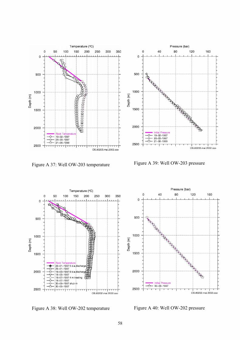
Figure A 39: Well OW-203 pressure Figure A 37: Well OW-203 temperature
Figure A 40: Well OW-202 pressure Figure A 38: Well OW-202 temperature
58

APPENDIX B1
Results of the update of 3-D natural state model
(In the Figures below, the dashed lines represent estimated formation temperature and pressure, filled black stars are values obtained from Bodvarsson and Pruess, (1987), and the open squares connected with lines are the model update from this work. The label on top of the pressure data refer to the element from which the well is located)
Figure B1 1: Calculated temperature and pressure for well OW-5
Figure B1 4: Calculated temperature and pressure for well OW-401
Figure B1 5: Calculated temperature and pressure for well OW-305
Figure B1 2: Calculated temperature and pressure for well OW-8
Figure B1 6: Calculated temperature and pressure for well OW-307
Figure B1 3: Calculated temperature and pressure for well OW-801
59

Figure B1 7: Calculated temperature and pressure for well OW-23
Figure B1 11: Calculated temperature and pressure for well OW-306
Figure B1 8: Calculated temperature and pressure for well OW-27
Figure B1 12: Calculated temperature and pressure for well OW-713
Figure B1 9: Calculated temperature and pressure for well OW-34
Figure B1 13: Calculated temperature and pressure for well OW-720
Figure B1 10: Calculated temperature and
pressure for well OW-705 Figure B1 14: Calculated temperature and
pressure for well OW-203
60

Figure B1 19: Calculated temperature and
pressure for well OW-202 Figure B1 15: Calculated temperature and
pressure for well OW-302
Figure B1 20: Calculated temperature and
pressure for well OW-201 Figure B1 16: Calculated temperature and
pressure for well OW-308
Figure B1 21: Calculated temperature and
pressure for well OW-32 Figure B1 17: Calculated temperature and
pressure for well OW-706
Figure B1 22: Calculated temperature and pressure for well OW-101
Figure B1 18: Calculated temperature and pressure for well OW-715
61

Figure B1 27: Calculated temperature and
pressure for well OW-204 Figure B1 23: Calculated temperature and
pressure for well OW-301
Figure B1 28: Calculated temperature and
pressure for well OW-724 Figure B1 24: Calculated temperature and
pressure for well OW-703
Figure B1 29: Calculated temperature and
pressure for well OW-901 Figure B1 25: Calculated temperature and
pressure for well OW-501
Figure B1 30: Calculated temperature and
pressure for well OW-716 Figure B1 26: Calculated temperature and
pressure for well OW-R2
62

Figure B1 33: Calculated temperature and
pressure for well OW-701 Figure B1 31: Calculated temperature and
pressure for well OW-30
Figure B1 32: Calculated temperature and
pressure for well OW-21 Figure B1 34: Calculated temperature and
pressure for well OW-704
63

APPENDIX B2
Production history matching of the “best” exploitation model (The Figures below show the model match of the production history. The lines are the computed and the dots are measured)
Figure B2 1: Production from block A8 Figure B2 3: Enthalpy in block A8
Figure B2 2: Calculated pressure in
element 1A8 Figure B2 4: Calculated pressure in
element 2A8
64
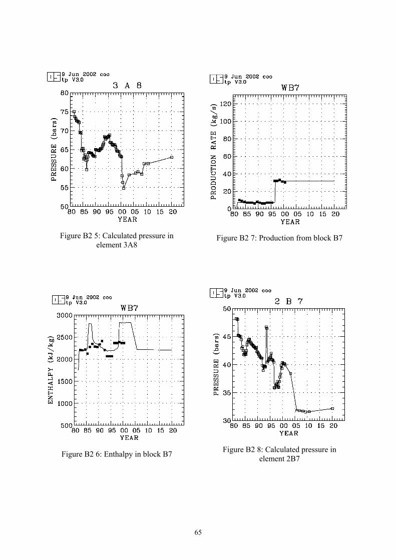
Figure B2 5: Calculated pressure in
element 3A8 Figure B2 7: Production from block B7
Figure B2 8: Calculated pressure in element 2B7 Figure B2 6: Enthalpy in block B7
65

Figure B2 9: Calculated pressure in element 3B7
Figure B2 11: Production from block B8
Figure B2 10: Enthalpy in block B8 Figure B2 12: Calculated pressure in element 1B8
66

Figure B2 13: Calculated pressure in element 2B8
Figure B2 15: Calculated pressure in element 3B8
Figure B2 14: Production from block B9 Figure B2 16: Enthalpy in block B9
67

Figure B2 17: Production from block C8 Figure B2 19: Enthalpy in block C8
Figure B2 18: Production from block C9 Figure B2 20: Enthalpy in block C9
68

Figure B2 21: Total production from the field
Figure B2 22: Average enthalpy in the field
69

APPENDIX C
Graphs of flow history of some wells from the Olkaria East production field
1980 1984 1988 1992 1996 2000 2004Year
0
2
4
6
8
10
12
Flow
rate
(kg/
s)
0
500
1000
1500
2000
2500
Enth
alpy
(kJ/
kg)Steam
WaterTotal massEnthalpy
1980 1984 1988 1992 1996 2000 2004
Year
0
2
4
6
8
10
12
Flow
rate
(kg/
s)
0
500
1000
1500
2000
2500
Enth
alpy
(kJ/
kg)
SteamWaterTotal massEnthalpy
Figure C 1: Output from well OW-2 Figure C 3: Output from well OW-11
1980 1984 1988 1992 1996 2000 2004Year
0
2
4
6
8
10
12
Flow
rate
(kg/
s)
0
500
1000
1500
2000
2500
3000
Enth
alpy
(kJ/
kg)
SteamWaterTotal massEnthalpy
1984 1988 1992 1996 2000 2004Year
0
2
4
6
8
10
12
14
Flow
rate
(kg/
s)
0
500
1000
1500
2000
2500
3000
Enth
alpy
(kJ/
kg)
SteamWaterTotal massEnthalpy
Figure C 2: Output from well OW-10 Figure C 4: Output from well OW-15
70

1980 1984 1988 1992 1996 2000 2004Year
0
5
10
15
20
25
30Fl
ow ra
te (k
g/s)
0
500
1000
1500
2000
2500
3000
Enth
alpy
(kJ/
kg)
SteamWaterTotal massEnthalpy
Figure C 5: Output from well OW-16
1984 1988 1992 1996 2000 2004Year
0
4
8
12
16
Flow
rate
(kg/
s)
0
500
1000
1500
2000
2500
3000
Enth
alpy
(kJ/
kg)
SteamWaterTotal massEnthalpy
Figure C 6: Output from well OW-19
1980 1984 1988 1992 1996 2000 2004Year
0
2
4
6
8
10
12
Flow
rate
(kg/
s)
0
500
1000
1500
2000
2500
Enth
alpy
(kJ/
kg)
SteamWaterTotal massEnthalpy
Figure C 7: Output from well OW-22
1980 1984 1988 1992 1996 2000 2004Year
0
2
4
6
8
10
12
14
Flow
rate
(kg/
s)
0
500
1000
1500
2000
2500
3000
Enth
alpy
(kJ/
kg)
SteamWaterTotal massEnthalpy
Figure C 8: Output from well OW-18
1980 1984 1988 1992 1996 2000 2004Year
0
2
4
6
8Fl
ow ra
te (k
g/s)
0
500
1000
1500
2000
2500
3000
Enth
alpy
(kJ/
kg)
SteamWaterTotal massEnthalpy
Figure C 9: Output from well OW-21
1980 1984 1988 1992 1996 2000 2004Year
0
2
4
6
8
Flow
rate
(kg/
s)
0
500
1000
1500
2000
2500
3000
Enth
alpy
(kJ/
kg)
SteamWaterTotal massEnthalpy
Figure C 10: Output from well OW-23
71

APPENDIX D
Solution to the discretized equations Solution by Newton’s method Let the solution vector be defined by x = (D1) T
NN xxxx ),,...,( 21221 −
where x1 =
11+nP , x2 = T (or ) are the primary variables at element i, x1
1+n 1
1+nS 2(j-1)+1, x2(j-1)+2 at
element j etc. The residual equations can then take the form R = f(x) = 0 (D2) where f = (f1, f2,, ..., f2N)T. Let xk+1 be the value of x at the (k + 1)th iteration; then xk+1 = xk + ∆xk for k = 0,1,2, ... (D3) If xk+1 is an approved approximation to x then f(xk+1) = f(xk + ∆xk) ≈ 0 Applying an n-dimensional Taylor’s series expansion gives, f(xk+1) = f(xk + ∆xk) = f(xk) + ∇ f(xk) ∆xk + ... neglecting higher order terms in (∆xk)2 gives f(xk+1) = f(xk) + J(xk)(xk+1 – xk) ≈ 0 (D4) where J(xk ) is the Jacobian matrix of the system given by
Jij =
∂∂
j
i
xf
for i = 1,2, ..., n and j = 1, 2 ,3, ...., n (D5)
evaluated at xk. If xk+1 is a solution then Rk+1 = f(xk+1) = 0 and we obtain xk+1 = xk – J-1(xk)f(xk) (D6) If the matrix J(xk ) is singular, then the inverse J-1(xk) cannot be calculated. This method has two major disadvantages:
(1) Convergence may not be achieved unless the initial approximation is a good one. (2) The method requires the user to provide the derivatives of each function with respect
to each variable. The user must therefore provide n2 derivatives and any computer implementation must evaluate the n functions and the n2 derivatives.
This method is therefore not appropriate for solving large problems.
72

Solution by conjugate gradient method The conjugate gradient method provides a powerful means for solving linear equation systems with positive definite symmetric matrices. A matrix A is symmetric and positive-definite if Aij = Aji and xTAx > 0 for any x ≠ 0. Let Equation D4 be written in the form Ax = b (D7) where A is symmetric positive-definite (in our case, the Jacobian matrix), x is the solution vector (x = xk+1 – xk) and b is the residual. Given an initial guess x0 at the solution, the conjugate gradient method generates a sequence of increasingly improved approximate solutions x1, x2, ...., residuals corresponding to the approximations and search directions. Iteration terminates when the error is deemed small enough or has reached a preset value. Solving Equation D7 is equivalent to problem of minimizing the quadratic form
f(x) = 21 xTAx - xTb (D8)
Minimization of D8 is achieved when x = A-1b. That is when ∇ f(x) = b - Ax = 0 (D9) Writing D9 in residual form gives r = b – Ax (D10)
The approximate solution x(i+1) is computed by x(i+1) = x(i) + 1+iα p(i+1) (D11) where α is the search parameter chosen to minimise f(x(i+1)) along the direction vector p(i+1). The new residual form of equation D10 gives r(i+1) = b – Ax(i+1) (D12) and substituting D11 in D12 and solving, we obtain
1+iα = (r Ti ri)/(p i ApT
1+ i+1) (D13) The vector p(i+1) is determined from the criterion that successive directions of search should be A-conjugate (orthogonal). This implies that p i ApT
j = 0 for i j (D14) ≠
73

Also, P has to be orthogonal to r. The vector p(i+1) therefore relates with ri by p(i+1) = ri + 1+iβ Pi (D15) where
1+iβ = (r Ti ri)/(r T
i r1− i-1) (D16)
74