NASA-CR-17420219860003825

A Reproduced CopyOF

Reproduced for NASA

by the

NASA Scientific and Technical Information Facility

L[8RARY COpyOCT 9 fJ86

1.l,HGLEY RESEARCH CENTERLIBRARY, NASA

/iAMP.TOfIf, YIRGINIA..

FFNo 672 Aug 65

DEPARTMENT OF MECHANICAL ENGINEERING AND MECHANICSSCHOOL OF ENGINEERINGOLD DOMINION UrnIJEHSiTYNORFOLK) VIRGINIA 23508

NUMERICAL SOLUTIONS OF NAVIER-STOK~S EQUATIONS. FOR A BUTLER WING

By

Jamsh1d S. Abolh3ssani) Graduate Research Assistant

and

S. N. Tiwari) Principal Investigator

Progress ReportFor the period ending August 31) 1985

Prepared for theNationa.l Aeronautics and Space Ac:ministrdtionLangley Research CenterHampton) Virginia 23665

Undel".Research Grant NCCl-68Dr. Robert E. ~nith, Jr., Technical MonitorACO-Computer Applications Branch

Submitted by theOld Dominion University Research FoundationP.O. Box 636 c

Norfolk, Virginia 23508

Uctobel' 1985

FOREW~ .J

This is a progress report on the research project II Numer-i cal Solutions

of Navier-Stokes Equations for a Butler Wing." The period of performance on

this research was January 1 through August 31, 1985, The work is supported, ." by the NASA/Langley Research Center through Cooperative .A.greement NCCl-68,

and monitored by Dr. Robert E. Smith, Jr., of the Analysis and Computat'ion

Division (Computer A?plications Branch), NASA/Langley, MS/125.

I .I'

i i

:.:~il'I

ABSTRACT

The flow field is simulated on the surface of a given delta wing

(Butler wing) at zero incident in a uniform stream. The simulation is done

by integrating a set of flow field equations. This set of equations governs

the unsteady, viscous. compressible, heat conducting flow of an ideal gas.

The equations are written in curvilinear coordinates so that the wing

surface is represented accurately. These equations are solved by the finite

difference method, and results obtained for high-speed freestream conditions

are compared with theoretical and experimental results.

In the present study, the r,avier-Stokes equat ions are solved nunerical-

:' ly. These equations are unsteady. compressible, viscous, and three-dimen-

.siona1 without neglecting any terms. The time dependency of the governing

equations allows the solution to progress naturally for an arbitrary initial

guess to an asymptotic steady state, if one exists. Th e e'1uat ions are

transformed from physical coardinates to the computational coordinates,

allowing the solution of the governing equations in a rectangular parallele­

piped domain. The equations at'e solved by the l"acCormack time-split tech-

nique which is vectorized and programmed to run on the CDC VPS 32 computer.

The codes are written in 32-bit (half I'lOrct) FORTRAN, which providE: an ap-

proximate factor of two decrease in computational time and doubles the

memory size co,npared to the 54-bit word size.

iii

~(~i ,

~_jJ£~~4r:f;~lWf,~f;~~~~1if~~~~B!l,i;t~;~Ir~~~~1~1;1~~I~:121~m~~!~~;~~~1

TABLE OF CONTENTS

Pa~~FOREWORD........................................................... 11

ABSTRACT ,. • • • • • • • • • • • • iii

1. INTROOUCTION ................ •., ••••• " "••••••• ,"............... 1

2. GOVERNING EQUATIONSlt •••••••••••.~ •••••• " •••• " •••••••••••• ·•••• , •• 3

3. METHOD OF SOlUTION............................................. 9

tkr- .~~!,(r: ....L .~

•:/

4i INITIAL AND BOUNDARY CONDITIONS., •••••••••••.••••••••••••••••••

5. APPLICATION TO A BUTLER WING .

6. RESULTS AND D[SCUSSION ••••••••••••••••••••••••••••••••••••• ~ •••

7. CONCLUDING REMARKS ••••••••••••••••••••••••••.••.•••••••••••••••

REFERENCES ..

11

14

15

17

18

APPENDIX A: MATHEMATICAL DETAILS FOR THE GOVERNING EqUATIONS...... 34

LIst OF FIGURES

Figure

1a Physical Model of a Butler Wing.............................. is

lb Cross-section of the Butler Wing along st~eamwise

direction ,. ".... 20

lc Coordinate system for the Butler Wing ........ \............... 21

2a Grid arrangement for the butler ~iing......................... 22

2b Grid arrangement viewed from the origin...................... 23

2c Grid distribution at Station One............................. 24

2d Grid distribution at- Stat10n Eleven ...... ... ,:.,.. .. ~ ...........

2e r,tid distribution at Station Sixteen .....•..•....••.••. _.•...••

2f Grid distribution at St(.tion T\·ienty-Six ......., ••••••.•......•

29 Grid distribution at Stacion Thirty-one .......•••.•••.•.....••

2h Grid distribution at Station Thirty-s'ix .......•..•..••....•..

25

26

27

28

29

.. '

iv

TABLE OF CONTENTS - continued -

Figure

2i Grid distribution at Station Forty-one ••••••.••.••••• ••••••••

3a Pressure coefficient along the center line ..••••••••••••• ••·•

3b Pressure ratio at 41.67% of chor~ ••.•••••.•.••••••. •••••··•••

3c Pressure ratio at 68.33 %of chord •.••..•••.••••••• •••••·••••

,.r[-

~

LIST OF FIGURES continued

Page

30

31

32

33

OJ

NUMERICAL SOLUTIONS OF NAV lEH··STOKES EQUATIONSFOR A BUTLER WING

By

J. S. Abolhassani 1 and S. N. Tiwari 2

1. INTRODUCTION

The Butler wing is a delta wing which was proposed by D. S. Hutler

(Ref. 4). The planform of the body h an isosceles triangle, and the lead­

ing edges of the wing are laid along the fviach lines of the undistutbed

stream. For the first 20% of the length, the body is a right circular cone.

The remainder of the body has elliptic sections which become more eccentric

as the sharp trailing edges are approached •

. D. S. Sutl er has compared experimental resu'lts for surface pressure

with theoretical values obtained by using a characteristic method to inte-

grate a:1 approximate form of the inviscid equations of motion (Ref. 4).

Butler used the hypersonic slender body theory approximation to simplify the

full equations of motions. Walkden and Caine estimated tne pressure on the

surface of a Butler wing at zero incid.ent in a steady uniform stream by

ntrnerically integrating the two semi-characteristic forms of equations which

govern the inviscid supersonic flow of an ideal gas with constant specific

heat (Ref. 5). Squire obtained experimental results for a Butler wing at

different Mach numbers and different angles of attach (Ref. 6,7). All

previous nLU11erical investigations have used inviscid equations and have

excluded the i~ake region. In contrast:, this study investigates the wake

region as well as the effect of viscosity on the flow. The fr·sults of ttlis

study are compared with availc:tJle experimental and nunerical rEsults.

lGraduate Research Assistant, Department of Hechanici En~lineering andMechanics, Old Dominion University, Norfolk, Virginia 2350B.

2Eminent Professor, (K!partment of \",pcnaniciil Engineering and ~iechanics, OldDominion University, Norfolk, V'rgiriia 23508.

,'.

ft~.'.

In order to study the flm'i arounu a Butler wing. the Navier-Stokes

equat ions are solved nlioerically. These equations are unsteady. compress­

ible, viscous, and three-dimensional without neglecting any terms. The time

dependency of the gover~ing equations allows the solution to progress natur­

ally from an arbitrary initial ~Juess to an as}1llptotic steady state. if one

exhts. The equations are transformed from the physical coordinates to the

computational coordinates. allowing the solution of the governing equations

in a rectangular parallelepiped domain. TI1(~ equations are solved by the

McCormack time-split technique which is vectorized and programmed to run on

the CDC VPS 32 (CYBER 205) computer. The codes were written in the 32-bit

(half-word) FORTRAN which provides an approximate factor of two. decrease in

computer time! and doubles the memory compared to the 64-bit word size.

2. GOVERNING EQUATIONS

The governing equations for a thermal fluid syster'll are the conserva,.~on

of mass, momentum, and energy. These equations are developed for c:n artli­

trary region assuming the system is in continuum. Equati~(lS of motiun for

viscous, compressible, unsteady, heat conducting flow CJn be written as:

Continuity: (2.1)

Momentum: ~ + v • (puu - ''1') :: 0, (2.2)

can be neglected if the pressure in a fluid is not cllanged abruptl.y dur"ing

(2.4a)

(2.3)+ v •a(E)

atEnergy:

bulk viscosity (k) by t~e expression k:: 2fl/3+IJ'. The contribut'ion of k

where E v2is the total energy per unit volume given by E :: p (e + - +

2

potent i a1 energy + ••• ) and e is Ule i nterna1 energy per unit vol ume.

where 6ij is the Kronecker delta function. and u' is the second coeffi­

cient of visc05ity. The two coefficients are related to the coefficient of

Equations 2.3 can be simplified by assuming that the stress at a point 'is

1inearly dependent on the rate of strain (deformation) of the fluid (New­

tonian fluid),

3

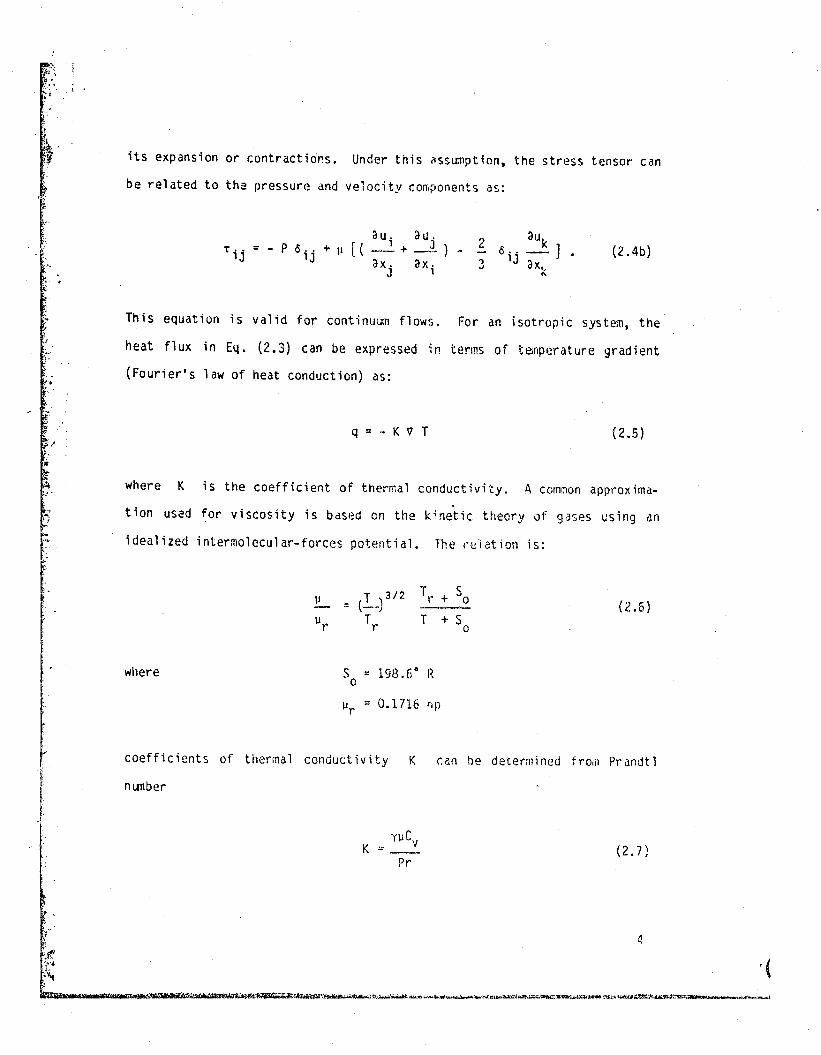
l~.··..v its expansion or contractions. Under this ~ssumption. the stress tensor can

rbe related to the pressure and velocity components as:

2 aUk<5 •• _J

? lJ "x" a k

(2.4b)

This equation is valid for continuum flows. For an isotropic system, the

heat flux in Eq. (2.3) can be expressed in terms of temperature gradient

(Fourier's law of heat conduction) as:

where K is the coefficient of thermal conductivity. A Cornt:1on approxima­

tion used for viscosity is bast~d on the k'netic theory of gases using dn

idealized intermolecular-forces potential. l~e relation is:

(2.5)q=··KVT

(2.6)

where So = 198.6° R

lJ r = 0.1716 np

coefficients of thermal conductivity K r.an be determined from Prandtl

nLITlber

(2.7)

where Cv is the specific heat at constant volume and y is the ratio of

specific heats.

It is necessary to have a supplementary relation to close the system of

equations CEq. (2.1) - (2.3)). By neglecting intermolecular forces (a ther­

mally perfect system). the,"modynamic properties can be related as:

P :: pRT (2.S)

where R is the gas constant. Thermally perfect gas assumpt ion allows

expression of the internal energy (e) as a function of T only [e :: e{T)].

In addition. assumption of calorically perfect £las [e{O) :: 0.\ allows the

following relation:

e ::: r~ Tt·v •

A combination of Eqs. (2.8) and (2.9) results in

(2.9)

P :: pe (y-1). (2.10)

these equations (Eqs. (2.1) - (2.3)) are in conservative form. For sim-

plicity, these equations can be expressed into e. compact vector form as:

\~here

au OF aG aH- + -- + -- + ....-' :: 0,at ax ay az

e, ~'. "~' ... ~.

t2.11)

5

-(

(2.12)~+at

For the sake of generality, we can ~ransform these equations from a pnysical

domain to a computational domain as

,, \

.. ~

p pUPU PUU - 'xx + P

U .- PV F = puv ,'. xy(~

PW puw - 'xzF~.; .l E Eu + qx - ~x + Pu

.' ." pv pw

..[ puv - , puw - Tyx zxG = PVV T + P H =: pvw - T

Y:l zyPV'" - TyZ pWW ~, + Pzz. .Ev + qy - ~y + Pv Ew + qz - ~z + Pw

+ r'y

aG.-.31;

The transformation coefficients can be computed fr~n a functional re-

lation between the computational coordinates and the physical coordinates.

x ;: x(I;,n.1;), y:= y(E;,n.r;). ard z:t Z(E;.I1,i;}. (2.13)

6

IfEq. (2.14) is known. the transformation coefficients can be computed by

direct differentiation. If the former relat,on is not k'1own, after some

algebraic manipulation, the transformation coefficients ~an be comruted by:

~~ ....•

f •

r. = r. (X t Yt Z) • n:: 1') ( X• Y. Z) t and 1;" d x t Y, z) • {2.14}

~ ~ ~l ax ax 1 .. 1ax--.ax ay Clz :31; an al;

an 3n an'" [J] = 3y ay 3y (2.15)ax 3y az aE; en 3e;

~ ~ !f.. az az azax 3y az ar. an al;

and IJ-l I are defined as (see Appendix A)ay 3z _ 3y ~) -(~: ~!:. - ~: ~~) (~3Y _ .~~) 1(-an ?r; 3r; an an <ll,; ar; dl) an cC; 3r; on

"ii

ol!o .' ~.

.:. \

where [J]

. 1 3yl,,] = -- -(--

IJ-l I ar.

l(2.1or.

az 3y Clz..- - ---)al; 31; Cl(

az ay dZ,-. --)

an Cln dE;

(~: ~ __3':"~)dl; ClI; 31; d(

-(~: ~ - !.: .~~)(lr. an Clr. elF.

( 3X 3y ax ay)-_._-----aE; or, al; dr.'

(~ ay _~ a1)al; an a" a~ J

(2.16 )

•t,I ax ax ax

aE; an ar;

1J··1 I =ay ay ayar. an al;

ilz Clz

~Ja~ df) 31;

7

-(,

..: .

,'..

t'

:0dX (lY al _ ay az ax (ay a;:: ~ 3y ~)-) -at 3n Clr,; aI;; 3n an a( al; al; 3(

+ ax (~ az 'Oy ~)31; Cl( an an aE;

In the present case, the planes of grid are perpendicular to the x-direction

thus allowing us to write:

x = x( () (2.17)

y '" Y(n,l;) (2.18)

z = Z(l1,I;). (2.19)

This reduces the metlA·ic coefficient flom nine to five non-zero elements.

8

3. METHOD OF SOLUTION

A time marching method is used to compute the solution. This a~lows us

to capture the possible transient feature. This method is an exp1 icit

second-order accurate time-sp1 it predictor-corrector algorithm [3J. The

governing equations (Eq. (2.12)) \are di scret i zed 1n comput at iana1 di rec-

tions. In a compact form, they can be expressed as

where

ll.t = fitn r;

1:; _ ~t~

2

and l.l; • Ln '

respect i ve1y.

and Lr; are the operators in ~. n. and r; directions,

A time step is completed in this algorithm with the appli-

cation of each operator applied symmetrically about the middle opey'atoy'.

For example, operator L~ can be defined as

LI:' (HI:') = Uout.... i ,j,k

where

Predictor step:

(3.2 a)

uini,j, kU.. k

1 .J ,

+ (H. ­1

lIt~ [.-- (F.-F· 1)

M; 1 1-

H , aF,:). I' - 11- az j,k

flF. i + (G. - G. 1) ~i. iax 1 1- 'dy

... ;..... ',,' --..

(3.2b)

9

Corrector ste.E.=..

uout; ,j, k = 1

2(3.2c)

+ (G 1'+1. - G.) ~ i + (H, 1 - H.) .~~ 1'), ay· ,+ 1 a Z 'k,.

This method has a time step stability limit, but there is no rigorous sta­

bility analysis a... ailable for this. A conservative time step that is corn··

monly used is

~t < min [1:1 + 1:1 + J:1 + C6.x 6.y t.z

(3.3)

where c is the local speed of sound.

In the supersonic region, there exists a large gradient which requires

a very fine mesh to resolve it. If they are not resolved, they produce a

large oscillation which eventually blows up the !clution. These osci J-

lations of "low frequency" can be suppressed by addin9 a fourth order darnp~

ening. A common dampening used is the pressure da,inpening. This can be

expressed in physical coordinates as

I" \ + C9..-----4P

R. •• 1,2,3 (3.4 )

where 6 1 == f;, 02 n, (';nd \ 3 == 1;.

10

4. INITIAL AND BGU~DARY CONDITIONS

In computational fluid dynamics the initial conditions usually con'e~

spond to a real initial situation for a transient pl"oblem, or a rough guess

for a steady state problem. In practice. initia', conditions are obtained

from experiments, empirical relations, approximation them"leS, or previous

computational results. An inappropriate initial guess may result il'1 yener-

ating unphysically strong transient waves which propagate through the compu­

tational region dominating the flow field and eventually lead to a solution

failure. In general, ttlere are two important requirements that should be

considered in the choice of initial conditions. First, they should be com­

patible with the fixed upstream boundary conditions. Secondly, the initia'i

conditions should be as physically close as possible to the actual nature of

the 'flow field in the region under study. The former wili m~nimize the

nunber of i terat ions required for convergence. An attractive approach is to

initialize the entire now field (including the upstre~ boundary and the

body surface) with a crude and simple guess (e.g., free stream condition).

Then, during the course of the computation, both bQdy and upstre~n boundary

conditions are chdnged in a gradual manner to their final values over a

prescribed n\J1lber of iterations. The former approdch is applied in only one

step which is equivalent to impulsive initial conditions.

It is equally important to implement a realistic, accurate, dnd stable

method to determine boundary cunditions. The application of certain condi.

tions may cause numerical instability even though the flow is. physical1y

stable. There dre neither mathematical nor physical justifications to irn-

ple;;'lent a realistic bOIJndary condition. t,jcst of the boundar'j conditions

currently implemented are drawn nli).in 1y upon intuition, wind tunnel experi,.

ence, and computational experimentation. There ,~re three general types of

11

/-::.

/

boundary "0ndl~ion:,. rl~Y al'e Di r',chlet ccnditions (specified function

value}, '~ellO',:ao c~IrHi ,tiCiiS (specific ,d rlvrmal gradien:.), and Roo'in condi-

tions (a clllTItinat:on (;f bot:,). Four important factors ShOUld be considered

in toe ,:~)edio:l of lJJ..;;:Jary ::0nditions. They arc convergence, stability,

computer time, and abovF: all the pili's ical justification.

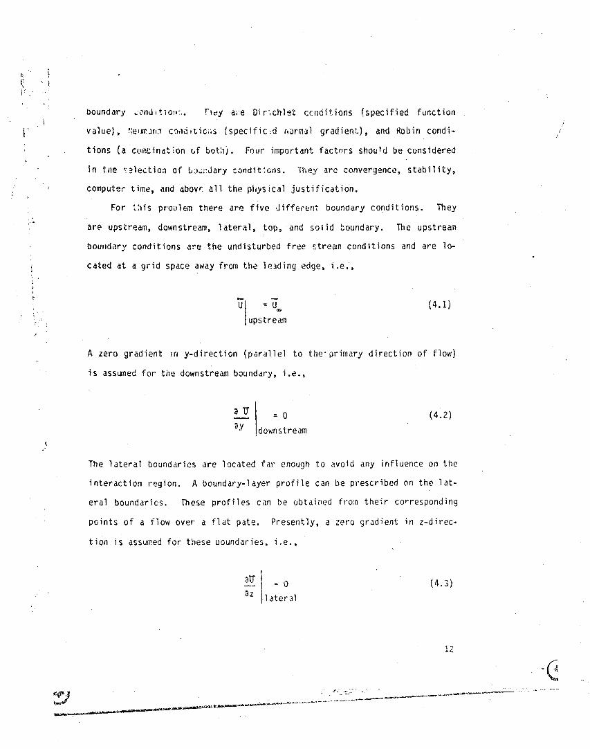
For t:lis proL'let1l there arc five Jifferent boundary conditions. They

arE' upstream, downstream, 1ateral, top, and so I id boundary. TIle upstream

boundary conditions are the undisturbed fr~e ~tream conditions and are 10-

cated at a grid space away from the le3ding edge. i.e.,

//

iii ~ U. upstre:m

(4.1)

A zero gradient in y-direction (parallel to the' primary direction of flow)

is assumed for tne downstream boundary, i.e.,

3 U'

3y::: 0

downstream

(4.2)

The lateral boundaries are located far enough to avoid any influence on the

interaction region. A boundary-layer profile can be prescribed on the lat­

eral boundaries. These profiles can be obtained from their corresponding

points of a flow over a flat pate. Presently, a zero gradient in z-direc-

tion is assumed for these boundaries. i.e.,

,aU I 0-I"az 11 ateral

(4.3)

12

l',

The wall is assumed impermeable and nO-51 ip boundary conditions are

appl ied. therefore. all velocity components are assumed to be zero. The

wan is also assumed to have it constant temperature Tw. A zero normal

pressure gradient is assumed for the solid surface, i.e.,

!f.1::o.3n Isolid

(4.4)

",< !I ,, i; 1.. 1: I~t :

I

!

"

~ !

This evaluation may appear to be based on the boundary-layer approximation

(zero normal pressure gradient). In fact. it is a muCh milder approxima­

tion. since constant pressure is not applied through the coundary layer but

over one grid line in the boundary layer. This approximation has yielded

stab.le computations for both non-separated and separated 90undary 1ayers

[2]. From Eq. (A.25b). Eq. (4.4) can be expressed as

/

+ n 2 + n2 + n2~ y z Pn

(' ')112n~ + n~ + n~

o (4.5)

13

·!.~. "'.:/"/ \1\

~ '.

i~

L,,

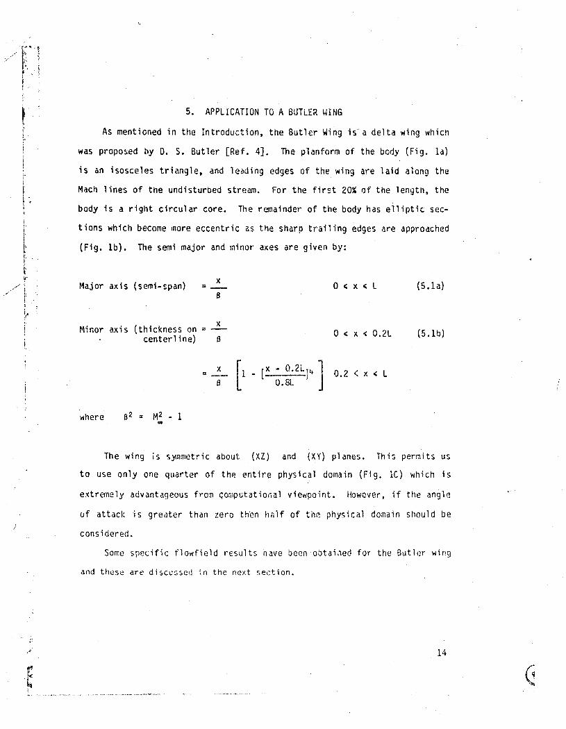
5. APPLICATION TO A BUTLER WING

As mentioned in the Introduction. the Butler Wing is a delta wing which

was proposed by D. S. Butler [Ref. 4]. The planform of the body (Fig. la)

is an isosceles triangle. and leading edges of the wing are laid along the

Mach 1ines of the undisturbed stream. For the first 20% of the length. the

body is a right circular core. The remainder of the body has elliptic sec­

tions which become more eccentric as the sharp trailing edges are approached

(Fig. lb). The semi major and minor axes are given by:

,iff ~,..ItI..Lt[1'

/ / ~,,'.'

Major axis (s emi - span) x=

B

Minor axis (thickness on x::-

centerline) B

o c; x c; L

o <: x " O.2L

(5.1a)

(5.1b)

where

= x

B [1 - [x - O.2L]4] 0.2 < x c L

0.8L

The wing is s)lnmetric about (Xl) and (XY) planes. This permits us

to use only one quarter of thE'! entire physical domain (Fig. 1C) which is

extremely advantageous ff'om Gomputatior.al viewpoint. However, if the angle

of attack is greater than zero th~n half of the physical domain should be

considered.

Some specific flowfield results nave been obtai~ed for the Butler wing

and these are discussed in the next section.

14

5. RESULTS AND DISCUSSION

Grid generation is the very first-step which should be considered in

entire face of the parallelepiped. A C-type grid is used in the present

work. However, the solid boundary is not mapped onto an entire face of the

obtaining flowfie1d solution over any cQnfigurat ion. Due to the data base

NetJerthe1ess, this maps the sol id boundary onto anthe trai 1ing edge.

into a parallelepiped. Jlmong the grid types, selection of an O-type grid

would produce a point sin~ularity at the tip and a line singularity aloflg

management of our program, it is necessary to map the entire physical domain

computational box. This creates a potentiai proolem in u;:>dating the oound­

ary conditions.

In this study, a two boundary grid generation (TBGG) technique develop­

ed by R. E. Smith [1] is used. The method is essentially an algebraic

method. The application of the TBGG method requires that the entire body be

. sliced into different cross-sections (Fig. 2a-b). The cross-sections of

wing are obtained in the stream-wise direction by analytical descriptions of

the wing sudace (Eq. S.l). The TBGG method ther, is used to generate the

,'"i i

rIi

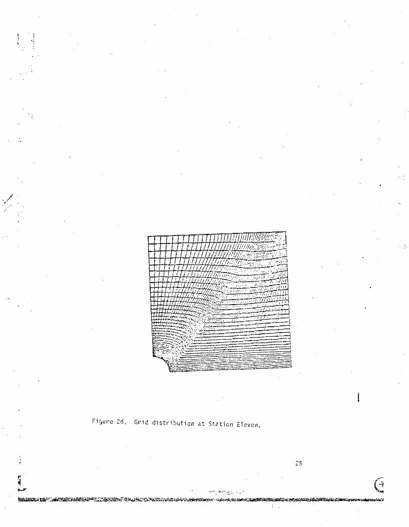
grid for each station. There are fifty.. five stations in the stream-wise

direction, and each station has 64 x 36 grid points (Figs. 2C-2i). fnere is

a total of 126.720 grid points which take 2.8 mi 11ion 32-oit ~Iords of pri­

mary memory (16 variables). The computational time required is 1.9 x 10- 5

sec/grid point/ iteration (2.5 sec/iteration). This is a typical require-

ment for the CYBtK 205 witt, tl'iO pipes.

Results are obtained for a Butler wing at t~.,. '" 3.5. Reo> = 2 x lOb/ft,

To> '"' 390 u R. Tw = 10noR. L = 0.8 ft. and zero an91(; of atta.ck. The com­

puted pressures are plotted in Fig. 3. TIle pressure coefficient a'iong the

center line is shown in Fig. 3a. The results ate cO~ipared with available

15

,.t'::~ _ •.•,:'

/

-j

i, I

experimental and nunerical results (Refs. 4,6.7). The resu1 ts are in excel­

1ent agreement with the experimental results of Ref. 4. !'bt-eovcr. they are

closer to the experimental results than previous nllner-ical results (Refs.

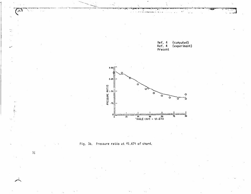
4.6,7). Pressure ratios are plotted at constant chordwise position against

the conical spam"ise coordinates (41.66% and 613.33%). 'n,ese arc seen to be

in good agreement wi th experimental and nlji'nerfcal results (Fi g. 3b-c).

In the near future, extensive results will be obtained for different

There are~ however. s~ne discrepancies in the results between 30G and 60°.

Thi!: might be due to the fact that grids are not orthogonal near those

regions.

,r"~~

~i:t·,.-,

•, ..,~

I,

",!

r

I"'·

i .~

f·!!

, I

fr~estre<¥1l conditions.

report.

These wi 11 be reported on in a future progress

II 'I'I.

f',~~L

16

(

.~.

,r

7. CONCLUDING REMARKS

General formulations are presented to investigate the flowfield over

complex configurat"ions forh"igh-speed freestrewl' conditions. I1Jl ,dvanced

~lgebraic method is used to generate gl"ids around these confiqurations. The

computational procedure developed is appl ied to investigate the flowfield

over a Butler wing. Illustrative resul ts obtained fo,' specified freestrearn

conditions compare very well with available experimental and numerical

results. Further studies, however, are needed to establish the validity and

versatility of the present code. After such model validations, it is anti­

cipated to use the co~e to investigate flowfield over complex confi~urations

such as closed-bluff bodies (i .e., circu1 ar and ell iptical c.y1 inders on a

flat plate, etc.).

, 71,

"'.. -:-

('\

.',.

"" .~..

.. ~

t·

REFERENCES

1. Smith, R.E •• "Two-Boundary Grid Generation for the Solution of theThree-Dimensional Compressible Navier-Stokes Equations," NASA TechnicalMemorandum 83123. May 1981.

2. Roache, P.J .. Computational F.lu.id Dynami.S2.' Hermosa pUblisher, 1972.

3. MacCormack, R.W. and Bl adwin, 6.5., "A Numerical Metil0d for Solving theNavier-Stokes Equations with Appl ication to Shock-Boundary Layer Inter­actions," AIM Paper 75-1, AIM 13th Aerospace SCiences lv\eeting, Pasa­dena, CA, January 20-22, 1975.

4. Butler, D.S •• "The Numerical Solution of Hyperbolic System of PartialDifferential Equations in Three Independent Variables," Proceedings ofthe Royal Society, Series A Mathematical and Physical SCiences, No.1281, vol 255, 232 .. 252, Apri 1 1960.

5. Walkden, F. and Caine. P•• "Surface Pl'essure on "i Wing 11::>vi09 withSuperson"ic Speed," Proceedings of Royal Society of London, Series A,volume 341, pp. 177-193, 1974. .

6. Squire. L.C., "Measured Pressure Distributions and Shock Shapes on a, Butler Wing," Cambridge University, Oepartment of Engineering, CUED/A­Aero/TR9. 1979.

7. Squire. L.C .. "Measured Pressure Distributions and ShOCK Shapes on aSimple Delta Wing," the Aerondutical Quarterly. volume 32. part 3. pp.188-198, August 1981.

18

..

;

r,.(

frf .!

Figure lao Physical Model of a Butler Wing.

19

,<.~'

/' J

{-._--------::....

X -L-L_-. I '.

xI'f

Figure lb. Cross-section of the BUt1CI' V/ing along streilm;dise direction.

20

,~ .. _..,.--.....,..,.~~- .... "-_. ..--

y

>z

Figure Ie. Coordinate system fJr the Butler Wing.

f-.1N

Figure 2a. Grid arrangement for ~he Butler Wing.

r",,.,.)

fi glJre 2b.Grid arrangement viewed fro~ the origin.

,

Figure 2c. Grid distribution of Station One.

./.t .'.

Figure 2d. Grid distribution at Station Eleven.

25

Figure 2e. Grid distribution at Station Sixteen.

26

\, 1

, '

Fi gure 2f. Gr}d distr"b "lUt1 Oil a j. (' ... t'lor Jt..O 10n T\'ientY-$ i x.

27/

I'

. '.., f

Figure 29. Grid distribution at Station Thirty-one.

;,' .- _.,.-._ .... .. ~ !4_. ••,.•;_.---~._:""'.-....-.••--..-.-. ,,I' ,...

(~

, .

.•r,, '\: j, I

i

/

---,....,--.--~- .... .. - --_.__._----_._-- '--..------.::::=.:::::::::::=-.-=--====------,.==:.::::--==::--===--=..::7"_=::===-..:::=:=:--=::---==.::"..=:::::=::::.=:=:::===

Figure 2h. Grid distrib~;tion at Station rhi,':/-s;x.

~'QC..I

_ •• __ ._~ ~4 ._~_~_.-;~- ~ ••

//

./

~.' :tI;

trI

~ln

I "

/

Figul'e 2i. Grid distritution at :.;tiltion Fo,-ty-one.

30

.' I

~I ~..~I ..,..

f-f't

t'. ~

~.i~

!f!

'\ ,

...zw-u-10.10.

~U

o Ref. 6<$> Ref. 7(, Ref. 4

P,'esent

oo

,w.u1.l.UJ ,III lll.u.uu.u.l U I I ! I , u1.JJ.W.,UJ~~.......................... .::'.3 .50 .67 •It" 1.00

RXlr-lL OISTRNCE f. XiCl

,I,

.'

./ ,/

Figue 3a. Pressure coefficient along the cente~ line.

31

-e

",

Ref. 4Ref. 4Present

(computed)(experiment)

.'

Fig. 3b. Pressure ratio at 41.67t of chord.

fI..i':" l..'~•. f,

,>I "

.'

/~ .1,-,t·

•

o Ref. 4<I Ref. 4

Present

(computed)(experiment)

I .

o:::.--_,-,-,.-,cr--~

o uw.w.J.J.u!! I I I ,I I I II! t ill IUU 1I1l/J.u.,W Ill! IUll,! I I.:.do ~ ~ ~ m ~ ~

~ (X/C :;; S8.33"~

0-/' ...~ 1.Sll/ .. ;f

. ~

f. 's,4, _,'"

~,"

rf.I!i

r

." i

, ,

Figure 3c•. Pressure ratio at 68.33% of chord,

33

APPENDIX A

MATHEMATICAL OETAILS FOR THE GOV£RN1~G E0UATIONS

A.l Curvilinear Coordinates

In covariant coordinate~ system (xi)' the position vector of a point

from the origin is eApressed as

,I

~ = ei xi - el Xl + e2 X2 + e3 X3 (A.1 )

tr!rr!

fIf!-f

r4I

t

is the local value of the ratio of an elemental vollMe in th~ physica'j

(usually dislorted) cell to the correspondingelelflental volume in ttle mapped

(cubiC) cell.

The contravarLmt bose vectors ill'e defined as

34

;

or

e1 /;x F. y ~; z1;\ i

e2 = "x "y11 I :.:. [J] j (A.3 )

z II

e3 I:; x Cy r: xJ II k

Position vector Cdn be expressed explicitly in terms of contravariant

ivector (x ); however the infinitesirn,d vector dr can be expressed as

,

fI

f.•rfr

ar ; idr ~ --- d x ~ e i dx

ax i

also the magnitude of arclength (ds) can be expressed as

where 6kt

is the kronecker delta,

(A.'+)

(A.S)

if

if

k - .f.

k t L

\

I>

Substitution of Eq. A.4 into Eq. A.S will result in

35

ds2 "'(e e )'d d 'i' J' x. X·"'9··C1xdx, :I lJ i j

where 9·· is call:>d c .lJ <;: ovanant fundamental metric coefficients.

These coefficients can be defined as

'. .~

axkaxk

9ij.. [J_l] I (J-l] :;: - .

oXi 3x.

J

They are defined as

911 :: x2 +~ + z2~ ( ~

912 :: 921 ;;; x Xn + Yt; Yll + -.; .c.~ Zn913 :: 931 II X x, + y Y, .. Z z,:~ .; .;922 :: x2 + '" + Z2n ~ n923 :: 932 :Ill Xn Xi; + YI'1 Y~ + z lr.:n933 :: x2 + ., + z2

l; .~ l;

Similarly co ..• variant fundamental metric f~'coe T1cients are defined as

gij[J]T

ax dXi<.. ei . e. :: [,JJ kJ

:: --- •3x i ax j

(A.6)

(A.7)

(A. 8 a)

(A.8b)

(A.8c)

(A.8d)

(A.H~)

(A.Sf)

(A.9)

or

gIl :: (2 + (2 + (lx Y lg21 '" 912 :;: E; + to

(A.1Oa)'1 I'l + Cx x .. 11

913y J' z z (A .10b)

:;: 931 '" r ex + r z: + f;'x 'y y "zz (A.lOcY922'" 11 2 -t 1')2 + n2

X y 'z(A.IVd)

36

.-' .. ~. ' ....,.(.~,~i'....

rj3

933

= 932 :: n 1; + 11 1; + nz i; L­X X Y Y

= ,..2 + r.2 + ,.2.. X • Y 'oZ

(A.lOe)

(A.lOf)

Furthermore, there exists a unique relationship between contravariant

and covariant fundamental metric coefficients,

i i 9rs 91s - 9rt 915G•.

9 .. = '-lJ

19 ij l 19· .\lJ

where

G = 9 9 2

11 22 339

23

G = G = 9 9 9 912 21 13 23 12 33

Ii = G = 9 9 - 9 913 31 12 23 13 22

G = 9 9 _92

22 11 33 13

G .:: G '" 9 9 - 9 923 32 12 1:1 :>3 33

G = 9 9_ 92

33 11 22 1.2

(A.ll)

(A.l2a)

(A.l2b)

(A.l2c)

(A.l2d)

(A.l2e)

(A.l2f)

There is also a relationship between covariant and contravariant base

vector

(A.13)

37

wnere 19 ij l ~ IJ-112

i.e.

or

wherei

,] " e

-(x z -x z )Tt:: I; Ii

(x~ zr,; - XI; z~ )

(x y -x y )n I; 1; Tt

-(X~YI;-XI;Y~) (A.14)

•.. 0"'

Thel-e is also a r~lationsl1ip between contravariant and covariant base'

vectors

~i =

i . e.

(A.IS)

or

- (~ Ii .F Ii )"x z 'z x

C"x!;;y-nix)

- ( F, xl'; y - F, f x ) (,~ .16a)

38

///.

I

(n/,z~T1Zl;y)

.. - (I'l l'; -I'l l'; )x z z x

('"fl- y.n/o x)

- (F./-z·F.l- y)

(cxl';z· ';Zl;X)

-(F;xr.iF:/-·,)

(r.l z·r. zl1y )

- (r. I'l -r. I'l ,X Z Z x·

(~ zT1 y-c.lx)

(A.16b)

The relationship between vector bases can be obtained also by matrix alge·

bra. Fr~o basic matrix identity. it can be written as

,"

[J] c [J-l]= Transpose of cofactor [~-l]

1J-1 1

* T= [[J-l] ]

\J-11(A.l?)

Equation (A.ll) is the same as Eq.(A.14).

There exists an inverse relation for Eq. (A.Il).

A.2 Vector Representation ,n Curvilinear Coordinates

A vector

ordinates as

F( F i, F j, F k) can be expressed in a c.ontravarientco-x y z

where

(A.18)

i "xiFi=~F +~_

ax x 'Oy

iF +~ F

y CZ 1(A.19)

Equation (A.19) can be expanded as

39

Ftl( )1/2

f;X F. y ~Z

[ F. iFX

911

1/2Fnl (9

22) = nx "y "z Fy = [J] Fy

F I (9 ) 1/2r.:

X 1;y 1;Z F Fl: 3J Z z

where 9ij is defined in Eq. (A.B).

(A.20)

The inverse relation to Eq. (A.20) is

I \ 1

- I ( 1/2) IF F 9x ~ 111/2

F = [J-1] 1-"'/ (922

)

FY r I (9 1/2)

. Z 1; 33

(A.21)

.'

-""

. I

For example, velocity vector in covariant coordinates can De written

as

I:L[J]-l

w IIlil (9ll

112) I./

VI (922 1I2 )J

IWI (9B 1/2)

Also, velocity vector in contravariant coordinates can be expressed as

1/2) IUVI (922)1/2 = [J] v

WI (933) 1/2 w

r UI (911)

1

Where u and U are velocities in covariant and cuntravariant coordinates

s.Ystem,

40

,.-.... ~a :?17rN~~R'lUtft~~od:~~~-'~~~.~~~~~f~.•W~":'~.:u;lUdI .... ....__.~...........l ........'t&l

., 'i: .' I •

. ,.. ,, .

/: ~

~.1

! .

A.3 Normal Derlvative in Curvilinear Coordinates

A normal derivative of a ~calar variable car be tamput~d as

,.".....

. !

where

VA = A i + A j + A Kx y. z

or

(A.23a)

(A.23b)

(A.23c)

/'.

A~A

11A

!;

(A.24a)

Eq~ation (A.23a) can be written as

3A_.- =an

co.lstant ljI

(A.24b)

For constant -~. Eq. (A.24b) can be written as

41

;.' "

3A

an

~

gIl A. + 912 A + g~3~A=_~. n.,/; C;

(11)1/2\9

(A.25~ -

.... ~_.•... f

For constant - 11. Eq. (A.24b) can be written as

For constant - c. Eq. (A.24b} can be written as

/(1 ., ,,,/

3A

3n11

aAan

=

+ 922 A + 92 ~ A11 C;

(922 ) 1/2

(A.25b)

(A .25c)

./

I

/.I

also~

• v

.//

/

.. 1

()

1/2

9ii\

3L gi j aA

j=l ClXi(A.26)

/

e.g.

(A) ~ ::n

1II

9

(A.27)

i<; A.4 Miscel1aneous Relations

Angle between t ....,o gl'jd lines '\s given by

12

i I./ /.

/

<' I . t~'.' ,

~.,

::_gu_~_Cos 6 ij 1/2

19'j i I 9jj I

therefore for orthogonal grid, the following should be true,

.., ~ j . (A.29) /.

; ,

:'./

I

;.,;~·t

Arclength is defined as

fArcl~ngth along x coordinate is defined d$

f 1/2 i(ds) ~ (9ii) dx.

iThe area of an element on which the x is constant is defined as

e.g.

dr~:: e2 dT1 x e3 d I; I = Gl1 dT'd!;

11dI" :: G22 dl;; dt;

(A.30a)

(/I .30b)

(A.31)

(A.32a)

(A.3ib)

43

I!

l

/'

( ./

. I.:~ , .

,.'

/, / /,

,,;/'>(- :I' ,', _

/ Ii.I ij :(,j ,

/

;",::,,' ;.'1

, t

'i

{,

Ii,(

/'

)/,/

-II'/'

Vo 1ume of an element is defi ned as

dV .. .Ci (x.!.:Y.!!l.:: IJ -1 I d~ dll dz:d(t,.'1.~)

/

df; dll dz;

I ,

(A.33)

44

"

!

!

/

I./1· / "

.I i

",. }

U1l

11111 IIIIII ~~\III\II~ 11\~~rrl~~\llrll[~~\11 1\ 11\ IIIIII 3 1176 01310 5490. -- .----- --- _._-----~-~~_.__.-