A Reinforcement Learning based Cognitive Approach for...

Dottorato di Ricerca in Ingegneria dei Sistemi (11046)

XXIV Ciclo

Settore Scientifico Disciplinare (SSD) Automatica (ING-INF/04)

Tesi di Dottorato:

A Reinforcement Learning based Cognitive

Approach for Quality of Experience Management

in the Future Internet

Relatore:

Prof. Francesco Delli Priscoli

Dottoranda:

Dott.ssa Laura Fogliati

Coordinatore del Dottorato:

Prof. Salvatore Monaco

Anno Accademico 2010-2011

1

Executive Summary

Future Internet design is one of the current priorities established by the EU. The EU

FP7 FI-WARE project is currently trying to address the issues raised by the design of the

Future Internet Core Platform.

This thesis aims at providing an innovative contribution to the definition of the Future

Internet Core Platform Architecture, in the frame of the “La Sapienza” University research

group activities on the FI-WARE project.

The reference architecture proposed by the “La Sapienza”University research group,

called Cognitive Framework Architecture, is based on two main elements, incorporating the

main “cognitive” functions: the Cognitive Enablers and the Interface to Applications.

The first goal of this thesis is the design of the Application Interfacearchitecture,

focusing on the key “cognitive” role of the Interface, related to the Application

Requirements Definition and Management. The Application Requirements are defined in

terms of Quality of Experience(QoE) Requirements.

The proposed Interface, called Cognitive Application Interface (CAI), is based on three

main elements: the Application Handler,the Requirement Agent and theSupervisor Agent.

The key element from the QoE perspective is the Requirement Agent: it has the role of

dynamically selecting the most appropriate Class of Service to be associated to the relevant

Application in order to “drive” the underlying network enablers to satisfy the target

QoElevelthat is required for the Application itself.

The QoEfunctionis defined taking into account all the relevant factors influencing the

quality of experience level as it is “globally” perceived by the final users for each specific

Application (including Quality of Service, Security, Mobility and other factors).The

proposed solution allows to manage single Applications assigning to them quantitative QoE

target values and “driving” the underlying network elements (enablers) to reach(or

approach) them.

The proposed approach models the QoE problem in terms of a Reinforcement Learning

problem, that is a Markov Decision Process, where the RL Agent role is played by the

2

Requirement Agent and the Environment is modelled as a Markov Process with a specific

state space and reward function.

Considering that the Environment model (network dynamics) is not known a priori, the

Author suggests to use “model-free” Reinforcement Learning methods, such as Temporal

Difference(TD) RL methods and, in particular, the Q-Learning algorithm.

The Cognitive Application Interface can be implemented in real network scenarios such

as fixedandmobile access networks, where resource limitations and bottlenecks are present,

because over-provisioning cannot be used, and specific network mechanisms and solutions

are necessary to guarantee the required Quality of Experience.

The second goal of this thesis is a concrete implementation of the proposed Cognitive

Application Interface, in order to test behaviour and performance of the proposed

Reinforcement Learning based QoE problem solution.

For implementation and simulation purposes, the QoS case has been considered: this is

a specific case, where the Application QoE is defined in term of Quality of Service

metrics.In the QoS case, throughput, delay and loss rateparametershave been

considered.The proposed QoE function assigns different weights to the QoS parametersand

allows to guarantee a satisfactory granularity in defining Application QoE requirements.

The considered network scenarios and the proposed Cognitive Application Interface are

implemented using the OPNET tool, a license-based SW platform that is widely used for

both academic and industrial applications in the ICT field.The network model is

implemented using a Dumbbellnetwork.The Supervisor Agent and the Requirement Agent

algorithms are implemented using the C++

language version supported by OPNET; in

particular, the Requirement Agent is implemented using a standard version of the Q-

Learning algorithm.

Several simulations have been run in order to test behaviour and performance of the

proposed Cognitive Application Interface and algorithms, considering single and multiple

application scenarioswith different network congestion levels.

In order to test the performance of the proposed solution, in each simulation scenario

“static cases”, where Classes of Services are permanently associated to the Applications,

are compared with “dynamic cases”, where each Requirement Agent dynamically selects

3

the most appropriate Class of Service to be associated to the relevant Application, in order

to “drive” the network elements to satisfy the required QoS level.

As known,traditional Quality of Service (QoS) management solutions typically operate

on a per-flow basis, permanently associating each application with a static Class of Service

andsupporting it on an appropriate flow, then managing traffic relevant to different

flows/classes with different priorities, without guaranteeing any specific Application target

QoS level.

The simulationresults clearly show that the dynamical Class of Service selection and

management, made possible by the co-ordinated action of the Supervisor and the

Requirement Agents, assures a significant improvement of the QoS performance of the

relevant Applications in relation to the traditional QoS approach, based on static Class of

Service mapping and management.

As known, the classic Q-Learning algorithm has impressive convergence properties,

but they are only guaranteed in single-agent scenarios: a promising hybrid solution for

overcoming the limitations of this algorithm when used in multi-agent systems, combining

it with a game-theory based approach, is the Friend or Foe algorithm.

Starting from this consideration, an alternative RL solutionhas been investigated in the

final part of this work, based on a two-Agent scenario, where each Requirement Agent plays

against a “Macro-Agent”, incorporating all the other Requirement Agents, and “learns to

act” using a FriendorFoe algorithm.

Some preliminary testshave been run on this solution, considering one of the

scenariosalready implemented for the standard Q-Learning version (in particular: a multi-

application scenario with medium congestion level): the obtained results show an

improvement in the algorithm performance, with respect to the standard version.

4

Thanks

First of all, a particular thank is due to Prof. Francesco Delli Priscoli, who proposed

me this opportunity to apply my never forgotten passion for mathematics, science and

innovation to something that is “concrete” and “useful” for the Future Internet

development.

The PHD study and research activities gave me the chance to integrate my educational

background (master degree in Mathematics in 1990) and professional carrier (in Telecom

Italia’s group companies, since 1991) with a new experience, very important and enriching

from the cultural, professional and human perspectives.

ICT Innovation, a key driver for the socio-economic development of European

Countries, requires a stricter collaboration between Industries and Academies and between

private and public organizations, as experienced in the most recent EU Programmes and

Initiatives.

I would like to express my thanks to my Company Management and the Human

Resources staff, for giving me the opportunity to collaborate with the University “La

Sapienza” during this thesis work on innovative ICT topics, related to the FutureInternet

design and development.

I would like also to thank the researchers and PHD students working in the “La

Sapienza” University research group coordinated by Prof. Delli Priscoli for their

collaboration on specific problems addressed in my thesis work, in particular Antonio

Pietrabissa, Vincenzo Suraci and Marco Castrucci.

A particular thank is due to Stefano Petrangeli and Marco Stentella for their support

during the implementation and simulation phase of this thesis work.

Finally, I would like to thank my family, and in particular my father, Alessandro, and

my brother, Vincenzo, the family’s “Engineer & Musician”, for their precious suggestions

and contributions.

5

Table of contents

Thesis Outline 8

List of Figures 10

1. INTRODUCTION 11

1.1. Future Internet: a view 11

1.2. Future Internet Architecture concept 14

2. COGNITIVE FRAMEWORK ARCHITECTURE 17

2.1. The Cognitive Manager 17

2.2. Potential advantages 19

3. APPLICATION INTERFACE ARCHITECTURE 22

3.1. Introduction 22

3.2. Key concepts underlying the Cognitive Application Interface 23

3.2.1. Applications supported by multiple micro-flows 29

3.3. Cognitive Application Interface architecture 30

3.3.1. Application Handler 33

3.3.2. Requirement Agent 34

3.3.3. Supervisor Agent 35

4. MARKOV DECISION PROCESSES 37


4.2. Stochastic processes 37

4.3. Markov chains 38

4.4. Properties of Markov chains 40

4.4.1. Long run properties of Markov chains 41

4.5. Continuous time Markov chains 43

4.6. Markov Decision Processes (MDP) 46

4.7. Multi-agent Markov Decision Processes 48

4.8. Partially Observable Markov Decision Processes (PO MDP) 49

5. REINFORCEMENT LEARNING 51


5.2. Elements of a RL system 52

5.3. The Reinforcement Learning Problem 55

5.3.1. Returns 56

5.3.2. Unified notation for episodic and continuing tasks 58

5.4. Modelling the environment as a Markov chain 58

5.4.1. Value functions 60

5.4.2. Optimal value functions 61

6

5.4.3. Optimality and approximations 64

5.5. Methods for solving Reinforcement Learning problems 64

5.5.1. Dynamic Programming (DP) 65

5.5.2. Monte Carlo methods 67

5.5.3. Temporal-Difference (TD) methods 69

5.5.4. TD prediction 71

5.5.5. Sarsa: on-policy TD control 73

5.5.6. Q-Learning: off-policy TD control 74

5.5.7. R-Learning: TD control for undiscounted continuing tasks 76

5.6. A unified view of RL methods: extended versions of TD methods 77

5.7. Multi-step TD Prediction 78

5.7.1. n-Step TD Prediction 78

5.7.2. The Forward View of TD(λ): λ-returns 80

5.7.3. The Backward View of TD(λ): eligibility traces 82

5.8. Learning and Planning methods 86

6. THE PROPOSED RL APPROACH 89

6.1. Why Reinforcement learning 89

6.2. Why Q-Learning 91

6.3. An alternative proposal: the Friend or Foe algorithm 92

7. COGNITIVE APPLICATION INTERFACE: THE PROPOSED RL

FRAMEWORK 96

7.1. Supervisor Agent 96

7.2. Requirement Agent 97

7.3. The Reinforcement Learning problem 98

8. COGNITIVE APPLICATION INTERFACE: THE QOS CASE 100

8.1. QoS Metrics and Requirement 100

8.2. Cognitive Application Interface: an example with QoS 101

8.2.1. Supervisor Agent in the QoS case 102

8.2.2. Requirement Agent in the QoS case 103

9. REAL NETWORK SCENARIOS 104

9.1. Fixed Networks 104

9.2. Mobile Networks 107

9.2.1. Cellular Network 107

9.2.2. Ad-hoc Network 111

10. IMPLEMENTED NETWORK SCENARIO 113

10.1. Simulation tool: OPNET 113

10.1.1. Key System Features 113

7

10.1.2. Typical Applications 115

10.1.3. Modelling Methodology 116

10.1.4. Editors and Tool 118

10.2. Model Specification 121

10.2.1. Network model: the Dumbbell network 121

10.2.2. QoS policy 122

10.2.3. Supervisor and Requirement Agent algorithms 123

11. SIMULATION RESULTS 130

11.1. Reference Scenario and key parameters 130

11.2. Single-Application Scenario 132

11.2.1. Traffic Scenario #1 133



11.2.4. Traffic Scenario #4 and #5 141

11.3. Multi-Application Scenario 145



11.4. Conclusions 151

12. AN ALTERNATIVE RL APPROACH: PROPOSED SOLUTION AND

PRELIMINARY RESULTS 152

12.1. Friend-or-Foe algorithm 152

12.2. Cognitive Application Interface implementation 153

12.3. Preliminary simulation results 156

13. CONCLUSIONS 158

References 161

ANNEX A – The Future Internet Public Private Partnership Programme 165

ANNEX B –OPNET Code 173

8

Thesis Outline

Chapter 1introduces the Future Internet main concepts, illustrating the main limitations

of the present Internet design, and presents the innovative “cognitive approach” proposed

by the “La Sapienza” University research group working on the UE 7FP FI-WARE project.

The FI-WAREprojectand the wider Future Internet PPP Programmearedescribed in Annex

(Annex A).

Chapter 2 expands on a possible architecture which could realize the above mentioned

cognitive approach. In the proposed architecture, called “Cognitive Future Internet

Framework”, the key “cognitive” roles are played by the Cognitive Enablers (CE) and by

the Application Interface.

Chapter 3proposes a possible architecture of the Application Interface,focusing on the

key cognitive function of the Interface, that is defining proper Application requirements and

solving the Quality of Experience (QoE) management problem. In the proposed

architecture, called Cognitive Application Interface (CAI), the key role is played by the

Requirement Agents. Each Requirement Agent has the role of dynamically selecting the

most appropriate “Class of Service” to be associated to the relevant Application in order to

“drive” the underlying Network Enablers to satisfy the Application Requirements and, in

particular, the target QoE level.

Chapters 4 and 5 illustrate the theoretical framework considered in this thesis work,

introducing the Markov Decision Processesand the Reinforcement LearningProblem and

describing possible approaches and solutions.

Chapter 6 illustrates the proposed RL-approach for solving the QoE problem addressed

in this thesis work. Itexplains why the Reinforcement Learning approach has beenfollowed,

considering several alternative approaches and methods developed in Control and Artificial

Intelligence fields. Then, it illustrates why the Temporal Differenceclass of RL algorithms

and, in particular, why the Q-learning algorithm has beenchosen. Finally, it illustrates some

hybrid solutions combining Reinforcement Learning and Games Theory (Learning in

Games).One of these solutions (Friend or Foe algorithm) seems promising in terms of

overcoming some limitations of the RL (Q-Learning) approach when adopted in multi-

agent systems.

9

Chapter 7describes the proposed solution to implement the Cognitive Application

Interface, approaching and solving the QoE problem: for the reasons illustrated in the

previous chapter, itis modelled as a Reinforcement Learning problem where the RL Agent

role is played by the Requirement Agent. The Requirement Agent is modelled as a RL

Agent, with a properaction spaceand able to learn to make optimal decisions based on

experience with the Environment, that is modelled withan appropriate state space and

reward function.The RL Agent can be implemented using an appropriate model-free

Reinforcement Learning algorithm: for the reasons explained in the previous chapter, the

Q-Learning algorithm has been chosen.

Chapter 8 illustrates the Quality of Service (QoS) case, where the QoE is defined

through basic QoS metrics and parameters. The general Application Interface proposed in

chapter 8 is particularised in the QoS case, that is the object of the implementation and

simulation phase of this thesis work.

Chapter 9introduces some real network scenarios, considering fixed and mobile access

networks, and illustrates how the proposed Interface elements can be mapped on the

network entities.

Chapter 10 illustrates the implemented network scenario, describing the simulation tool

(OPNET) and illustrating the implemented Model Specification.

Chapter 11 describes the simulated scenarios and the main simulation results.Some

details on the implementation (OPNET code) are provided in Annex (Annex B).

Chapter 12 illustrates an alternative RL solution, based on a two-agent system, where

each Requirement Agent plays against a “Macro-Agent”, incorporating all the other

Requirement Agents, and “learns to act” through a Friend or Foe algorithm. A preliminary

simulation result is also presented: it seems promising in terms of improving the RL

algorithm performance.

Chapter 13 concludes the thesis, summarising the work and the results obtained,

illustrating advantages and limitations of the proposed approach and solutions and giving

recommendations for further improvements and future work.

10

List of Figures

Figure 1 - Proposed Cognitive Future Internet Framework conceptual architecture

Figure 2 - Cognitive Manager architecture

Figure 3 - Application Interface Architecture

Figure 4 - The agent-environment interaction in RL

Figure 5 - State and state-action pairs sequence

Figure 6 - Weighting given in the λ-return to each of the n-step returns

Figure 7 - Forward view of TD(λ)

Figure 8 - Backward view of TD(λ)

Figures 9 to 13 - Application Interface Architecture: fixed, cellular and ad hoc networks

Figure 14 - Dumbbell network

Figures 15 and 16 - Supervisor Agent: OPNET Node and Process Model

Figures 17and 18 - Requirement Agent: OPNET Node and Process Model

Figures 19 to 28 - Single Application Scenario - Traffic Scenarios from 1 to 5: Average

QoE -Static and Dynamic Case

Figures 29 to 32 - Multiple Application Scenario - Traffic Scenarios 1 and 2: Average QoE

-Static and Dynamic Case.

Figure 33 - Friend or Foe approach: The Macro-Agent

Figure 34 – Friend or Foe approach: preliminary simulation results

11

1. INTRODUCTION

1.1. Future Internet: a view

Future Internet design is one of the current priorities established by the UE. The EU

FP7 FI-WARE project is currently trying to address the issues raised by the design of the

Future Internet Core Platorm.

This chapter introduces the Future Internet main concepts, illustrating the main

limitations of the present Internet design, and describes the innovative cognitive approach

proposed by the “La Sapienza”University research group working on the FI-WARE project.

The FI-WARE project and the wider Future Internet PPP Programme are described in

Annex (Annex A).

First of all, a definition of the entities involved in the Future Internet, as well as of the

Future Internet target, can be given as follows:

• Actors represent the entities whose requirement fulfillment is the goal of the

Future Internet; for instance, Actors include users, developers, prosumers, network

providers, service providers, content providers, etc.

• Resources represent the entities that can be exploited for fulfilling the

Actors' requirements; example of Resources include services, contents, terminals,

devices, middleware functionalities, storage, computational, connectivity and

networking capabilities, etc.

• Applications are utilized by the Actors to fulfill their requirements and needs

exploiting the available resource; for instance social networking, context-aware

information, semantic discovery, virtual marketplace, etc.;

In the “La Sapienza” University research group vision, the Future Internet target is to

allow Applications to transparently, efficiently and flexibly exploit the available Resources,

aiming at achieving a satisfaction level meeting the personalized Actors’ needs and

expectations. Such expectations can be expressed in terms of a properly defined Quality of

Experience (QoE), which could be regarded as a personalized function of Quality of

Service (QoS), security, mobility,… parameters.

12

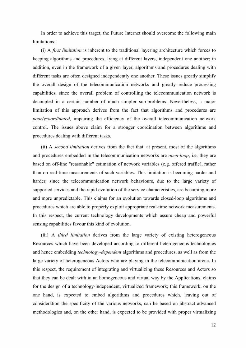
In order to achieve this target, the Future Internet should overcome the following main

limitations:

(i) A first limitation is inherent to the traditional layering architecture which forces to

keeping algorithms and procedures, lying at different layers, independent one another; in

addition, even in the framework of a given layer, algorithms and procedures dealing with

different tasks are often designed independently one another. These issues greatly simplify

the overall design of the telecommunication networks and greatly reduce processing

capabilities, since the overall problem of controlling the telecommunication network is

decoupled in a certain number of much simpler sub-problems. Nevertheless, a major

limitation of this approach derives from the fact that algorithms and procedures are

poorlycoordinated, impairing the efficiency of the overall telecommunication network

control. The issues above claim for a stronger coordination between algorithms and

procedures dealing with different tasks.

(ii) A second limitation derives from the fact that, at present, most of the algorithms

and procedures embedded in the telecommunication networks are open-loop, i.e. they are

based on off-line "reasonable" estimation of network variables (e.g. offered traffic), rather

than on real-time measurements of such variables. This limitation is becoming harder and

harder, since the telecommunication network behaviours, due to the large variety of

supported services and the rapid evolution of the service characteristics, are becoming more

and more unpredictable. This claims for an evolution towards closed-loop algorithms and

procedures which are able to properly exploit appropriate real-time network measurements.

In this respect, the current technology developments which assure cheap and powerful

sensing capabilities favour this kind of evolution.

(iii) A third limitation derives from the large variety of existing heterogeneous

Resources which have been developed according to different heterogeneous technologies

and hence embedding technology-dependent algorithms and procedures, as well as from the

large variety of heterogeneous Actors who are playing in the telecommunication arena. In

this respect, the requirement of integrating and virtualizing these Resources and Actors so

that they can be dealt with in an homogeneous and virtual way by the Applications, claims

for the design of a technology-independent, virtualized framework; this framework, on the

one hand, is expected to embed algorithms and procedures which, leaving out of

consideration the specificity of the various networks, can be based on abstract advanced

methodologies and, on the other hand, is expected to be provided with proper virtualizing

13

interfaces which allow all Applications to benefit from the functionalities offered by the

framework itself.

Some initiatives towards Future Internet are trying to overcome some of the above

described limitations, e.g., GENI [Ge], DARPA’s Active Networks [Da], argue the need for

programmability of the network components. Some other initiatives [Ch] extend this with

argumentation for declarative networking, where the behavior of a network component is

specified using some high-level declarative language, with a software-based engine

implementing the behavior based on that specification. Further results have been achieved

in [Te] where a Proactive Future Internet (PROFI) vision addresses interoperability of the

network elements programmed by different organizations, and the need for flexible

cooperation among network elements using semantic languages.

The most recent studies on Future Internet present only preliminary requirements [Ga]

and rarely try to propose feasible layered architectures [Va].

The innovative architectural concept proposed by the “La Sapienza” University

research group working on the FI-WARE project[see Ca]is illustrated in the nextparagraph,

expanding ideas preliminarily introduced in [De-1] and [De-2].

The need to manage heterogeneous resources, over heterogeneous systems, requires a

cognitive approach: a“cognitive framework”,based on semantic virtualization of the main

Internet entities, is proposed.

The next paragraph, outlines how the present Internet limitations can be overcome

thanks to the proposed Future Internet Architecture concept, based on the so

calledCognitive Future Internet Framework,which is a disruptive overlay, operated by

semantic-aware and technology neutral Enablers, where the most relevant entities involved

in the Internet experience converge in a homogeneous system by means of virtualization of

the surrounding environment.

By means of dynamic enablers and proper interfaces, the Cognitive Framework can

operate over heterogeneous environments, translating them into semantic-enriched

homogeneous metadata.The virtualization allows the Cognitive Framework to manage the

available resources using advanced, technology independent algorithms.

14

1.2. Future Internet Architecture concept

The concept behind the proposed Future Internet architecture, which aims at

overcoming the three limitations mentioned in the previous paragraph, is sketched in Figure

1. As shown in the figure, the proposed architecture is based on a so-called "Cognitive

Future Internet Framework" (in the following, for the sake of brevity, simply referred to as

"Cognitive Framework") adopting a modular design based on middleware "enablers".

The enablers can be grouped into two main categories: the Semantic Virtualization

Enablers and the Cognitive Enablers.

The Cognitive Enablers represent the core of the Cognitive Framework and are in

charge of providing the Future Internet control functionalities. They interact with Actors,

Resources and Applications through Semantic Virtualization Enablers.

The Semantic Virtualization Enablers are in charge of virtualizing the heterogeneous

Actors, Resources and Applications describing them by means of properly selected,

dynamic, homogeneous, context-aware and semantic aggregated metadata. Indeed in order

to overcome the increasing heterogeneity of Future Internet, it is necessary to describe the

different entities (i.e. Actors, Resources and Applications) by using a homogeneous

language based on a common semantic. There already exist theoretical solutions to cope

with semantic metadata handling (i.e. ontologies) and technological solutions (XML -

eXtensible Markup Language, RDF - Resource Description Framework, OWL - Ontology

Web Language, etc.). The use of semantic metadata allows to make an abstraction of the

underlying complexity and heterogeneity. Heterogeneous network nodes, applications and

user profiles can be virtualized on the basis of their homogeneous, semantic description. In

order to let a new entity be an asset of the Future Internet architecture, a correspondent

semantic virtualization enabler is needed in order to translate its technology dependent

characteristics (e.g. information, requirements, data, services, contents…) into technology

neutral, semantically virtualized ones, to be used homogeneously within the Cognitive

Future Internet Framework. The other way around, the Semantic Virtualization Enablers are

in charge to translate the technology independent decisions, taken within the Cognitive

Future Internet Framework, into technology dependent actions which can be actuated

involving the proper heterogeneous Actors, Resources and Applications.

The Cognitive Enablers consist of a set of modular, technology-independent,

interoperating enablers which, on the basis of the aggregated metadata provided by the

15

Semantic Virtualization Enablers, take consistent control decisions concerning the best way

to exploit the available Resources in order to efficiently and flexibly satisfy Application

requirements and, consequently, the Actors' needs. For instance, the Cognitive Enablers can

reserve network resources, compose atomic services to provide a specific application,

maximize the energy efficiency, guarantee a reliable connection, satisfy the user perceived

quality of service and so on.

Cognitive Future Internet Framework

Actors

Users

Network Providers

ProsumerDevelopers

Content Providers

Service

Providers

Ap

plica

tion

s

Semantic Virtualization Enablers

Cognitive Enablers

Identity, Privacy,

Confidentiality

Preferences, Profiling, Context

Multimedia Content

Analysis and Delivery

Connectivity

Resource

Adaptation &

Composition

Generic Enabler X

Generic Enabler Y

Generic Enabler Z

Resources

Services

Networks

Contents

Devices

Cloud Storage

Terminals

Computational

Figure 1- Proposed Cognitive Future Internet Framework conceptual architecture

Note that, thanks to the aggregated semantic metadata provided by the Semantic

Virtualization Enablers, the control functionalities included in the Cognitive Enablers have

a technology-neutral, multi-layer, multi-network vision of the surrounding Actors,

Resources and Applications. Therefore, the information enriched (fully cognitive) nature of

the aggregated metadata, which serve as Cognitive Enabler input, coupled with a proper

design of Cognitive Enabler algorithms (e.g. multi-objective advanced control and

optimization algorithms), lead to cross-layer and cross-network optimization.

The Cognitive Framework can exploit one or more of the Cognitive Enablers in a

dynamic fashion: so, depending on the present context, the Cognitive Framework activates

and properly configures the needed Enablers. In this respect,a fundamental Cognitive

Enabler, namely the so-called Orchestrator has the key role of dynamically deciding for

each application instance, consistently with its requirements and with the present context,

16

the Cognitive Enablers which have to be activated to handle the application in question, as

well as their proper configuring and activation/deactivation timing.

In each specific environment, the Cognitive Framework functionalities have to be

properly distributed in the various physical network entities (e.g. Mobile Terminals, Base

Stations, Backhaul network entities, Core network entities). The selection and the mapping

of the Cognitive Framework functionalities in the network entities is a critical task which

has to be performed case by case by adopting a transparent approach with respect to the

already existing protocols, in order to favour a smooth migration.

It should be evident that the proposed approach allows to overcome the three above-

mentioned limitations:

(i) Concentrating control functionalities in a single Cognitive Framework makes much

easier to take consistent and coordinated decisions. In particular, the concentration of

control functionalities in a single framework allows the adoption of algorithms and

procedures coordinated one another and even jointly addressing in a one-shot way,

problems traditionally dealt with in separate and uncoordinated fashion.

(ii) The fact that control decisions can be based on properly selected, aggregated

metadata describing, in real time, Resources, Actors and Applications allows closed-loop

control, i.e. networks become cognitive, as further detailed in the next chapter.

(iii) Control decisions, relevant to the best exploitation of the available Resources can

be made in a technology independent and virtual fashion, i.e. the specific technologies and

the physical location behind Resources, Actors and Applications can be left out of

consideration.In particular, the decoupling of the Cognitive Framework from the underlying

technology transport layers on the one hand, and from the specific service/content layers on

the other hand, allows to take control decisions at an abstract layer, thus favouring the

adoption of advanced control methodologies, which can be closed-loop thanks to the

previous issue. In addition, interoperation procedures among heterogeneous Resources,

Actors and Applications become easier and more natural.

17

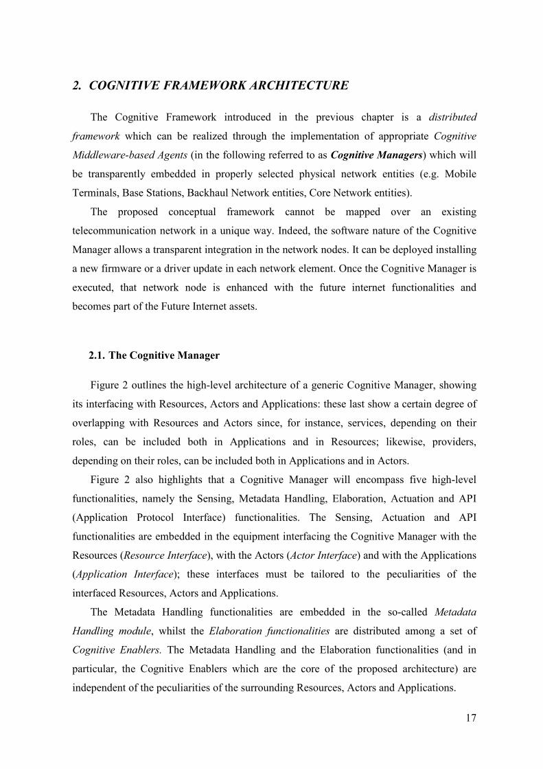
2. COGNITIVE FRAMEWORK ARCHITECTURE

The Cognitive Framework introduced in the previous chapter is a distributed

framework which can be realized through the implementation of appropriate Cognitive

Middleware-based Agents (in the following referred to as Cognitive Managers) which will

be transparently embedded in properly selected physical network entities (e.g. Mobile

Terminals, Base Stations, Backhaul Network entities, Core Network entities).

The proposed conceptual framework cannot be mapped over an existing

telecommunication network in a unique way. Indeed, the software nature of the Cognitive

Manager allows a transparent integration in the network nodes. It can be deployed installing

a new firmware or a driver update in each network element. Once the Cognitive Manager is

executed, that network node is enhanced with the future internet functionalities and

becomes part of the Future Internet assets.

2.1. The Cognitive Manager

Figure 2 outlines the high-level architecture of a generic Cognitive Manager, showing

its interfacing with Resources, Actors and Applications: these last show a certain degree of

overlapping with Resources and Actors since, for instance, services, depending on their

roles, can be included both in Applications and in Resources; likewise, providers,

depending on their roles, can be included both in Applications and in Actors.

Figure 2 also highlights that a Cognitive Manager will encompass five high-level

functionalities, namely the Sensing, Metadata Handling, Elaboration, Actuation and API

(Application Protocol Interface) functionalities. The Sensing, Actuation and API

functionalities are embedded in the equipment interfacing the Cognitive Manager with the

Resources (Resource Interface), with the Actors (Actor Interface) and with the Applications

(Application Interface); these interfaces must be tailored to the peculiarities of the

interfaced Resources, Actors and Applications.

The Metadata Handling functionalities are embedded in the so-called Metadata

Handling module, whilst the Elaboration functionalities are distributed among a set of

Cognitive Enablers. The Metadata Handling and the Elaboration functionalities (and in

particular, the Cognitive Enablers which are the core of the proposed architecture) are

independent of the peculiarities of the surrounding Resources, Actors and Applications.

18

Resources

Actors

Actuation functionalities

(enforcement)

Sensing functionalities

(monitoring, filtering,metadata

description)

Actuation functionalities

(provisioning)

Sensing functionalities

(monitoring, filtering,metadata

description)

Actor

Interface

Resource

Interface

Cognitive Manager

Metadata Handlingmodule

Elaboration functionalities

Control commands Resource related

information

Sensed metadataElaborated metadata

Elaborated metadata Sensed metadata

Application

protocols

Enriched

data/services/

contents

Actor related

information

Aggregated

metadata

(Present

Context)

Exchanged

metadata

TO

/FR

OM

OT

HE

R P

EE

R C

OG

NIT

IVE

MA

NA

GE

RS

Metadata handling

functionalities

(storing, discovery, composition)

Ap

plica

tion

Interfa

ce

Ap

plica

tion

s

Cognitive Enablers

AP

I fun

ction

alitie

s

Figure 2 - Cognitive Manager architecture

With reference to Figure 1, the Sensing, Metadata Handling, Actuation and API

functionalities are embedded in the Semantic Virtualization Enablers, while the Elaboration

functionalities are embedded in the Cognitive Enablers.

The roles of the above-mentioned functionalities are the following:

1. Sensing functionalities are in charge of (i) the monitoring and preliminary

filtering of both Actor related information coming from service/content layer (Sensing

functionalities embedded in the Actor Interface) and of Resource related information

(Sensing functionalities embedded in the Resource Interface); this monitoring has to

take place according to transparent techniques, for example by means of the use of

passive monitoring agents able to acquire information about the Resources (e.g.,

characteristic of the device, network performances, etc.) and about the Actors (e.g.,

user’s profile, network provider policies, etc.), (ii) the formal description of the above-

mentioned heterogeneous parameters/data/services/contents in homogeneous metadata

according to proper ontology based languages (such as OWL);

2. Metadata Handling functionalities are in charge of the storing, discovery

and composition of the metadata coming from the sensing functionalities and/or from

metadata exchanged among peer Cognitive Managers, in order to dynamically derive

the aggregated metadata which can serve as inputs for the Cognitive Enablers; these

19

aggregated metadata form the so-called Present Context;it is worth stressing that such

Present Context has an highly dynamic nature;

3. Elaboration functionalities are embedded in a set of Cognitive Enablers

which, following the specific application protocols and having as key inputs the

aggregated metadata forming the Present Context, produce elaborated metadatato be

provided to the Interfaces, aiming at (i)controlling Resource exploitation, (ii) providing

enriched data/services/contents, (iii) providing to the Interfaces information allowing to

properly drive and configure the API, Sensing and Actuation functionalities (these last

control actions, for clarity reasons, are not represented in Figure 2);

4. Actuation functionalities are in charge of (i) proper translation in

technology-dependent commands of the decisions concerning Resource exploitation and

enforcement of these commands into the involved Resources (Enforcement

functionalities embedded in the Resource Interface; see Figure 2); the enforcement has

to take place according to transparent techniques, (ii) proper translation in technology-

dependent terms of the data/services/contents elaborated by the Cognitive Enablers and

provisioning of these enhanced data/services/contents to the right Actors (Provisioning

functionalities embedded in the Actor Interface; see Figure 2).

5. API functionalities are in charge of interfacing the protocols of the

Applications, managed by the Actors, with the Cognitive Enablers. In particular, these

functionalities, also on the basis of proper elaborated metadata received from the

elaboration functionalities, should derive "cognitive" Application requirements (as

detailed in the following Chapter).

2.2. Potential advantages

The proposed approach and architecture have potential advantages which are

hereinafter outlined in a qualitative way:

Advantages related to effectiveness and efficiency

(1) The Present Context, which is the key input to the Cognitive Enablers,

includes multi-Actor, multi-Resource information, thus potentially allowing to perform

the Elaboration functionalities availing of a very "rich" feedback information.

(2) The proposed architecture (in particular, the technology independence of the

Elaboration functionalities, as well as the valuable input provided by the Present

20

Context) allows to take all decisions in a cognitive, abstract, coordinated and

cooperative fashion within a set of strictly cooperative Cognitive Enablers. So, the

proposed architecture allows to pass from the traditional layering approach (where each

layer of each network takes uncoordinated decisions) to a scenario in which,

potentially, all layers of all networks benefit from information coming from all layers

of all networks, thus, potentially, allowing a full cross-layer, cross-network

optimization, with a remarkable expected performance improvement.

(3) The rich feedback information mentioned in the issue (1), together with the

technology independence mentioned in the issue (2), allow the adoption of innovative

and abstract closed-loop methodologies (e.g. adaptive control, robust control, optimal

control, reinforcement learning, constrained optimization, multi-object optimization,

data mining, game theory, operation research, etc.) for the algorithms embedded in the

Cognitive Enablers, as well as for those embedded in the Application Interface. These

innovative algorithms are expected to remarkably improveboth performance and

efficiency.

Advantages related to flexibility

(4) Thanks to the fact that the Cognitive Managers have the same architecture

and work according to the same approach regardless of the interfaced heterogeneous

Applications/Resources/Actors, interoperation procedures become easier and more

natural.

(5) The transparency and the middleware (firmware based) nature of the

proposed Cognitive Manger architecture makes relatively easy its embedding in any

fixed/mobile network entity (e.g. Mobile Terminals, Base Station, Backhaul network

entities, Core network entities): the most appropriate network entities for hosting the

Cognitive Manager functionalities have to be selected environment by environment.

Moreover, the Cognitive Manager functionalities (and, in particular, the Cognitive

Enabler software) can be added/upgraded/deleted through remote (wired and/or

wireless) control.

(6) The modularity of the Cognitive Manager functionalities allows their

ranging from very simple SW/HW/computing implementations, even specialized on a

single-layer/single-network specific monitoring/elaboration/actuation task, to complex

multi-layer/multi-network/multi-task implementations

21

(7) Thanks to the flexibility degrees offered by issues (4)-(6), the Cognitive

Managers could have the same architecture regardless of the interfaced Actors,

Resources and Applications. So, provided that an appropriate tailoring to the

considered environment is performed, the proposed architecture can actually scale

from environments characterized by few network entities provided with high

processing capabilities, to ones with plenty of network entities provided with low

processing (e.g. Internet of Things).

The above-mentioned flexibility issues favours a smooth migration towards the proposed

approach. As a matter of fact, it is expected that Cognitive Manager functionalities will be

gradually inserted starting from the most critical network nodes, and that control

functionalities will be gradually delegated to the Cognitive Modules.

Summarizing the above-mentioned advantages, we propose to achieve Future Internet

revolution through a smooth evolution. In this evolution, Cognitive Managers provided with

properly selected functionalities are gradually embedded in properly selected network

entities, aiming at gradually replacing the existing open-loop control (mostly based on

traditional uncoordinated single-layer/single-network approaches), with a cognitive closed-

loop control trying to achieve cross-optimization among heterogeneous Actors,

Applications and Resources. Of course, careful, environment-by-environment selection of

the Cognitive Manager functionalities and of the network entities in which such

functionalities have to be embedded, is essential in order to allow scalability and to achieve

efficiency advantages which are worthwhile with respect to the increased

SW/HW/computing complexity.

22

3. APPLICATION INTERFACE ARCHITECTURE

3.1. Introduction

The architecture outlined in the previous sections highlights the key importance of the

Interfaces which, using as key input properly elaborated metadata, should be in charge of:

(i)properly selecting the heterogeneous information which is worthwhile to be

monitored and translating it in homogeneous metadata (sensing functionalities),

(ii) properly translating in technology-dependent commands the decisions concerning

Resource exploitation and enforcing these commands into the involved Resources

(actuation/enforcement functionalities),

(iii) properly translating in technology-dependent terms the data/services/contents

elaborated by the Cognitive Enablers and providing these enhanced data/services/contents

to the appropriate Actors (actuation/provisioning functionalities)

(iv) deriving proper "cognitive" Application requirements (API functionality).

This Chapter elaborates on this last role (iv) which will be performed by the

Application Interface and which, as explained in the following, introduces in the proposed

architecture a further important “cognition” level (in addition to the one of the Cognitive

Enablers); this is the reason why, in the following, we will talk about a "Cognitive

Application Interface".

At present, at each micro-flow supporting a given Application instance a (in the

following, for the sake of brevity, when referring to an "Application a", we mean an

"Application instance a") is statically associated (statically, means for the whole application

duration) a Service Classk(a), properly selected in the predefined set of Service Classes

which the considered network supports. The various network procedures are in charge of

guaranteeing to each Service Class a pre-defined performance level.

This approach has the inconvenient that, on the one hand, due to the very different

personalized Application QoE Requirements, in general, no Service Class perfectly fits a

given application, and, on the other hand, the static association between Applications and

Service Classes prevents the possibility to adapt to network traffic variations. In addition,

the fact that, at present, network control takes place on a per-flow basis, rather than on a

per-microflow basis, entails further problems related to control granularity.

23

In order to overcome these inconveniences, a dynamic association between

Applications and Service Classes is proposed: so, the Cognitive Application Interface, on

the basis of proper feedback information accounting for the present network traffic

situation, is in charge of selecting, at each time ts, for each microflow supporting a given

Application a the most appropriate Service Class, aiming at satisfying personalized

Application QoE Requirements.

3.2. Key concepts underlying the Cognitive Application Interface

First of all, it is necessary to introduce appropriate metrics related to the micro-flows

supporting the Applications. These metrics should refer to all the factors which can concur

in the QoE definition (e.g. QoS, security, mobility,…).

Application QoE Requirementsshould be based on these metrics.

The parameters should (i) be useful for assessing the Application QoE, (ii) be

technology independent, (iii) be so general as to encompass all kinds of possible

Applications, (iv) be complex enough to reflect all possible Application requirements, but

simple enough for not introducing useless complexity in the Cognitive Enablers which have

to manage them, (v) be,as far as possible, easily monitored by the Sensing functionalities.

Each in-progress microflow1 is associated to a Service Class. Traditionally, this

association is static (i.e. it just depends on the nature of the established micro-flow and it

does not vary during the microflow lifetime) and is made on a per flow basis. On the

contrary, in the proposed Cognitive Application Interface, this association will be dynamic

(i.e. it can be varied at each time instant ts): this entails remarkable advantages as explained

in the following.

As mentioned, according to the most recent trends, network control (as far as QoS,

security, mobility,... are concerned) is typically performed on a per-flow basis.

Let k denote the generic Service Class and K denote the total number of Service

Classes. As known, a Flow refers to the packets entering the network at a given ingoing

1By microflow we mean a flow of packets relevant to a given application and having the same requirements

(for instance, a bidirectional teleconference application taking place between two terminals A and B, is

supported by 4 microflows, i.e. an audio microflow from A to B, a video microflow from A to B, an audio

microflow from B to A, a video microflow from B to A).

24

node n ∈ N, going out of the network at a given outgoing node m ∈ N, and relevant to in-

progress connections associated to a given Service Class k ∈ K.

Each flow f is characterized by a set of Flow Requirementsrelated to QoS, Security,

Mobility, etc..Note that the fact that each Flow (and not just each single micro-flow) is

subject to a set of Flow Requirementslimits the complexity of the Elaboration

functionalities, since these functionalities have to operate on a per-flow basis, rather than on

a permicro-flow basis; in this respect, a given flow can aggregate many micro-flows. This

issue is essential for guaranteeing scalability.

In the following, without loss of generality, we assume to refer to given ingoing and

outgoing nodes, so that we can deal with a set of Service Class Requirementsmaking

reference to a set of Service Class Parameters identified by the selected metrics and to a

set of Service Class Reference Valueswhich characterize the Service Class in question.For

instance, in the QoS case, we propose the Service Class Requirements, Parametersand

Reference Values as defined in Chapter 8.

A key goal of the Elaboration functionalities included in the Cognitive Managers is to

control the available Resources in such a way that, for each Service Class k, the associated

Service Class Requirements are respected.

As mentioned above, in order to limit the complexity of the Elaboration functionalities,

which is essential for guaranteeing scalability, a limited set of Service Classes should be

foreseen.

For the sake of clearness, in the following, we will refer to the case in which an

Application is supported by just one micro-flow: as detailed in the next paragraph, we can

refer to this case without loss of generality.

At present, the mapping between Service Classes and Applications is statically

performed: this means that a given Application is permanently associated a given Service

Class, namely the one whose Service Class Requirements are expected, on average traffic

conditions, to better ”approach” the Application QoE Requirements.

The traditional static approach could be very limiting due to the following reasons:

(A) considering the very large amount of possible different Application QoE

Requirements, the QoE requirements of a given Application will not be, in general,

25

satisfied by any Service Class. Even more, the Application QoE Requirements can

even make reference to parameters not included in any set of Service Class

Parameters;

(B) the fact that network control is performed on a per-flow basis rather than on

a per-microflow basis can penalize some applications;

(C) the most appropriate mapping among Service Classes and Applications

should vary depending on the performance actually offered by the Service Classes

which could differ from the expected one due to various reasons (e.g. unexpected

traffic peaks relevant to some Service Classes, low performances of the Elaboration

functionalities, etc.).

The proposed solution intends to overcome the above-mentioned limitationsthanks to a

dynamic association between Applications and Service Classes.As a matter of fact, the

Cognitive Application Interface has the key role of dynamically selecting, on the basis of

properly selected feedback variables, the most appropriate Service Classes which should be

associated to the microflow supporting each Application instance (by "dynamical", we

mean that the selection will vary while the Application is in progress).

The key criterion underlying the above-mentioned dynamical selection is to approach,

as far as possible, a performance level meeting the personalized Application QoE

Requirements.

Up to the author's knowledge, in the literature, differentQoE models have been

proposed, following a passivenetwork-centric approach (with QoE “passively” measured

from QoS or other network-based parameters), an activeuser-centric approach (with QoE

“actively” derived gathering the user satisfaction) or a combination of them.The QoE

definition is a very critical and challenging task, because the “real” user experience is

highly subjective and dynamic.

In this respect, the approach followed in this thesis work is based on defining the

Application QoE Requirements by providing:

1) a QoE function ha allowing to compute for a given Application a, at each

time instant ts2, on the basis of a set of values assumed, at time ts (and/or at times prior

2We assume that network control takes place at time instants ts periodically occurring with period Ts(i.e.

ts+1= Ts+ts); the period Ts has to be carefully selected trading-off the contrasting requirement of more

frequently changing the Service Classes supporting the Applications (which allows a better fitting among the

26

to ts), by properly selected feedback variablesΘ(ts,a), the Measured QoE, experienced

by the Application a, hereinafter indicated as QoEmeas(ts,a):

QoEmeas(ts,a) = ha(Θ(ts,a))

2) a target reference QoE level, hereinafter indicated as QoEtarget(a), whose

achievement entails the satisfaction of the Actor using the Application a. This means

that if QoEmeas(ts,a)≥QoEtarget(a)the Actor in question is “satisfied”.

Note that the above-mentioned way of dealing with the Application QoE Requirements

has the key advantage of being extremely flexible since it leaves completely open the QoE

definition, allowing its tailoring to the specific environments and application types.

Note that even the feedback variables Θ(ts,a) can be flexibly selected depending on the

considered environment. They can be simply a proper subset of the Present Context;

alternatively, they can be deduced by specific Elaboration functionalities by a proper

processing of the Present Context.

For instance, the feedback variables Θ(ts,a) can consist of proper metadata representing

QoS/security/mobility performance measurements (e.g. delay or BER measurements);

following an active user-centric approach, also feedbacks directly provided by the users can

be considered.

We can now define the following error function:

e(ts,a) = QoEmeas(ts,a)− QoEtarget(a)

If the above-mentioned error is negative,at time ts, the Actor using the Application a is

experiencing a not satisfactory QoE (underperforming application). If the above-mentioned

error is positive,at time ts, the Actor using the Application a is experiencing a QoE even

better than expected (overperforming application). Note that this last situation is desirable

only if the network is idle; conversely, if the network is congested, the fact that a given

Application a is overperforming is not, in general, desirable, hence it can happen that such

achieved Application performance and the expected ones), with the requirement of limiting the complexity of

the Cognitive Application Interface (a more frequent updating means more demanding interface processing

capabilities).

27

Application is subtracting valuable resources to another application a' which is

underperforming.

In light of the above, the Cognitive Application Interface should dynamicallydetermine,

for each Application a,on the basis of (i) the monitoring of properly selected feedback

variables Θ(ts,a), and of (ii) the personalized Application QoE Requirements (expressed in

terms of the function haand of the reference value QoEtarget(a)), the most appropriate

Service Classk(ts,a) to be associated to the microflow supporting the Application in

question.

The goal of the above-mentioned dynamical selection is to avoid, as far as possible, the

presence of underperforming applications from the achieved QoE point of view; in case this

is not possible (e.g. due to a network congestion), the dynamical selection in question

should aim at guaranteeing fairness among applicationsfrom the QoE point of view (e.g. the

fact that a given application a should reach its QoEtarget(a) must not be got at the expenses

of another application a' going away from its QoEtarget(a')). More precisely, the dynamical

selection in question should aim at minimizing the errore(ts,a) for all the Applications

simultaneously in progress at time ts.

It is worth stressing that the above-mentioned Cognitive Application Interface task is

performed on the basis of selected feedback variables, which means that the Application

Interface becomes cognitive: this introduce in the proposed architecture a further level of

cognition, in addition to the one guaranteed by the Cognitive Enablers embedded in the

Elaboration functionalities.

It is fundamental also to stress that the proposed Cognitive Application Interface can be

used in conjunction with any type of Enablers (regardless of the fact that such Enablers are

cognitive or not) and these last can continue to operate according to their usual way of

working. As a matter of fact, the proposed Cognitive Application Interfaceintroduces the

"cognition" concept in a way which is completely decoupled from the Elaboration

functionalities and from the possible presence of Cognitive Enablers within these last

functionalities. In other words, thanks to the Cognitive Application Interface, the whole

Future Internet Framework becomes closed-loop (i.e. cognitive) regardless of the actual

way of working of the Enablers, which can be either open or closed loop.

28

Even more, the introduction of a Cognitive Application Interface is completely

transparent with respect to the other Cognitive Manager modules, i.e. its insertion does not

entail any modification of these last modules.

It is worth noting that the Cognitive Application Interface, by selecting a given Service

Class for a given Application a, implicitly selects the associated Service Class

Requirements; in this respect, remind that the (Cognitive) Enablers are in charge of driving

Resource exploitation so that these Service Class Requirements are satisfied. If the

(Cognitive) Enablers do not satisfactory perform their tasks, or, more in general, if the

(Cognitive) Enabler way of accomplishing their task is not satisfactory from the QoE point

of view, the Cognitive Application Interface should recognize such situation through the

monitored feedback variables and accordingly react, re-arranging Service Class selection.In

this sense, the Cognitive Application Interface can even remedy to possible (Cognitive)

Enablers deficiencies.

It is worth stressing that the presented dynamic approach allows to overcome the

above-mentioned limitations of the static one, due to the following reasons:

(A) the proposed approach allows to establish a plenty of different Application

QoE Requirements (thanks to the fact that the function ha is general); these

requirements can even make reference to parameters not included in any set of Service

Class Parameters(thanks to the fact that the feedback variables Θ(ts,a) are general);

(B) the fact that each Application can have its own Application QoE

Requirements (which is implicit in the Application QoE Requirement definition)

entails a per-microflow control;

(C) a proper selection of the feedback variables entails the fact that the Cognitive

Application Interface is able to perceive possible QoE performance impairments and

should properly react.

Clearly, all the above-mentioned desirable features are achieved only if the dynamical

selection of the most appropriate Service Class k(ts,a) is properly performed.

29

The proposed approach for performing this very complex task is based on the

implementation, at the Cognitive Application Interface, of appropriate closed-loopcontrol

and/or reinforcementlearning methodologies.

3.2.1. Applications supported by more than one microflow

In general, each Application a is supported by more than one microflow: let c1, c2,…,

cA denote the A microflows supporting the Application a.

Let QoEtarget(ci) i=1,…,A denote the Target Microflow Quality of Experience (QoE) of

the i-thmicroflow supporting the Application a. Such Target Microflow QoEs are defined

so that achieving the target QoE for all the connections supporting a given Application a

entails that the Target Application QoE, i.e. QoEtarget(a), is achieved.Let QoEmeas(ts,ci)

i=1,…,A denote the Measured Microflow Quality of Experience(QoE) of the i-

thmicroflowsupporting the Application a, at time ts (i.e. the QoE of the microflow ci

actually achieved at time ts).

The target of the Cognitive Application Interface is to make an appropriate control so

that QoEmeas(ts,ci) approaches, as much as possible, QoEtarget(ci) for any i=1,…,A, thus

entailing that the Measured Application QoE, indicated as QoEtarget(a), approaches the

Target Application QoE, i.e. QoEtarget(a).

Let hci denote the personalized function allowing the computation of the Measured

Microflow QoE relevant to the microflow ci (namely, one the microflows supporting the

Application a) on the basis of the feedback variables, i.e.:

QoEmeas(ts,ci) = hci(Θ(ts,a))

Let ga denote the personalized function allowing the computation of the Measured

Application QoE on the basis of the Measured QoEs of the supporting microflows, i.e.:

QoEmeas(ts,a) = ga(QoEmeas(ts,c1), QoEmeas(ts,c2),…, QoEmeas(ts,cA))

Note that, by construction:

QoEtarget(ts,a) = ga(QoEtarget(ts,c1), QoEtarget(ts,c2),…, QoEtarget(ts,cA))

30

since, as previously stated, the target microflow QoEs are selected so that achieving the

target QoE for all the microflows supporting a given Application a entails that the Target

Application QoE, i.e. QoEtarget(a), is achieved.

In order to achieve the Target Application a QoE, it is sufficient to achieve the

TargetQoE for all microflows ci i=1,…,A supporting the Application a.This issue allows to

decompose the problem of achieving the overall QoE for the Application a in A

independent sub-problems each one referring to a supporting microflow ci. This, in turn,

allows to refer, in the following of this document, to an Application a with just a single

microflow, without any loose of generality, thus also allowing a great simplification of the

notations which can directly refer to the application a instead of to the supporting

microflows. So, in the following, without loose of generality, we will simply refer to the

problem of dynamically selecting the most appropriate Service Class associated to the

Application a (more precisely, the most appropriate Service Class associated to the single

microflow supporting the Application a).

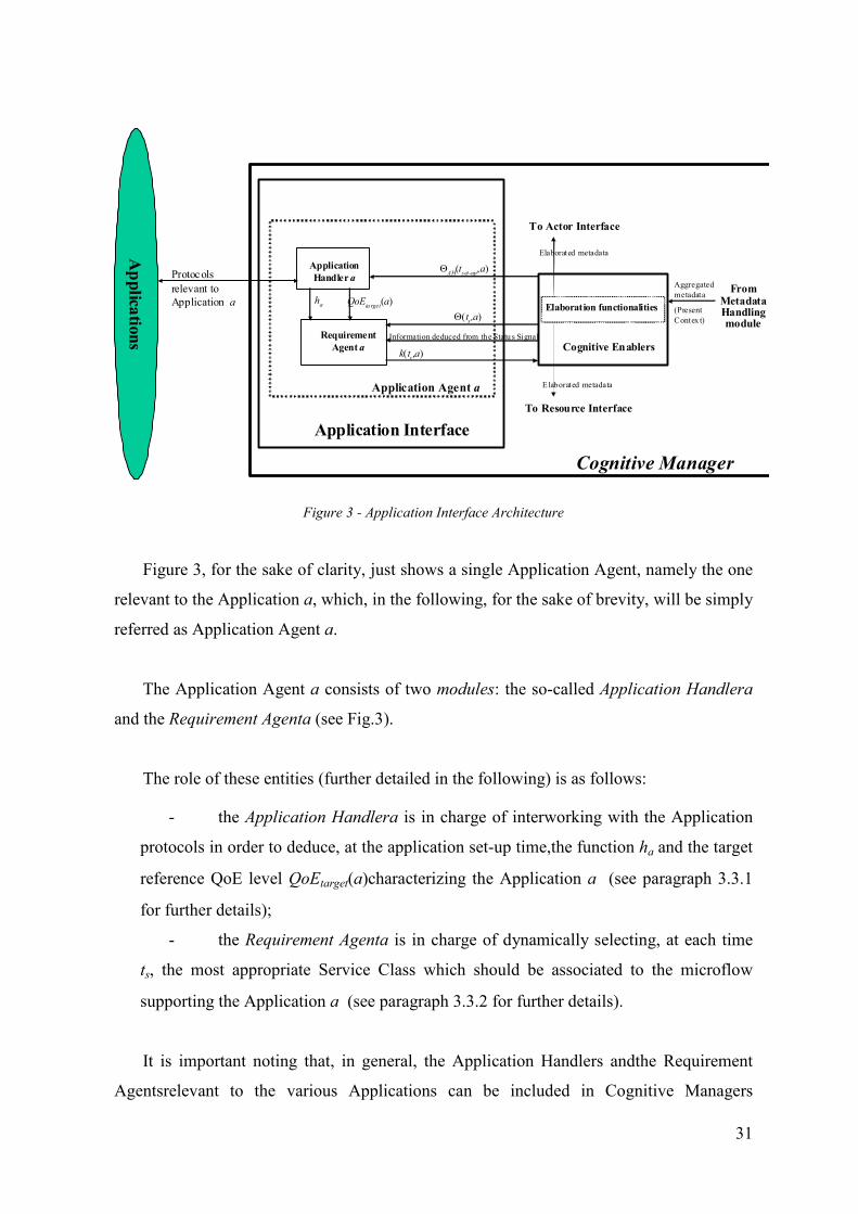
3.3. Cognitive Application Interface architecture

The proposed Cognitive Application Interface architecture of a given Cognitive

Manager is shown in Fig. 3, which is conceived as the explosion of the Application

Interface block appearing in Fig. 2.

The architecture is organized according to a number of Application Agentswhich are

embedded in the Cognitive Managers:each in progress Application a has its own

Application Agent.

In other words, at a given time, the number of Application Agents is equal to the

number of in progress Applications; this means that at each Application set-up a new

Application Agent is created and at each Application termination the relevant Application

Agent is deleted.

31

To Resource Interface

Cognitive Manager

FromMetadataHandlingmodule

Elaboration functionalities

E laborated metadata

Elaborated metadata

Protocols

relevant to

Application a

Aggregated

metadata

(Present

Contex t)

Application Interface

Ap

plica

tion

s

Cognitive Enablers

To Actor Interface

Application

Handler aΘ

AH(t

set-up,a)

Θ(ts,a)

ha

Requirement

Agent a

QoEta rget

(a)

k(ts,a)

Application Agent a

Information deduced from the Statu s Signal

Figure 3 - Application Interface Architecture

Figure 3, for the sake of clarity, just shows a single Application Agent, namely the one

relevant to the Application a, which, in the following, for the sake of brevity, will be simply

referred as Application Agent a.

The Application Agent a consists of two modules: the so-called Application Handlera

and the Requirement Agenta (see Fig.3).

The role of these entities (further detailed in the following) is as follows:

- the Application Handlera is in charge of interworking with the Application

protocols in order to deduce, at the application set-up time,the function ha and the target

reference QoE level QoEtarget(a)characterizing the Application a (see paragraph 3.3.1

for further details);

- the Requirement Agenta is in charge of dynamically selecting, at each time

ts, the most appropriate Service Class which should be associated to the microflow

supporting the Application a (see paragraph 3.3.2 for further details).

It is important noting that, in general, the Application Handlers andthe Requirement

Agentsrelevant to the various Applications can be included in Cognitive Managers

32

embedded in network entities (e.g. Base Stations, Mobile Terminals, etc.) which can be

placed at different physical, fixed or mobile, locations. The appropriate mapping of the

above-mentioned Handlers/Agents in the network entities is a delicate task which have to

be performed environment-by-environment; some instances of such mapping are provided

in Chapter 9.

In this respect, it is fundamental stressing that a key requirement of the conceived

architecture is scalability which can be assured, in consideration of the plenty of

Applications simultaneously in progress in a considered network, only imposing that the

signalling exchanges among Application Handlers,Requirement Agents and Supervisor

Agent must be kept limited: otherwise, the network will be overwhelmed by the signalling

overhead.

In particular, the Requirement Agents, which are in charge of dynamic tasks, should

perform their decisions independently one another, without exchanging information one

another. Clearly, this issue entails a very complex problem of coordination among the

Requirement Agents of the considered network, since a Requirement Agent has to take

decisions which impact on the utilization of Resources shared with other Requirement

Agents without knowing the decisions taken by these last. In this respect, note that a

Requirement Agent relevant to a given Application, by selecting, at a time ts, a given

Service Class for the micro-flow supporting the Application, also automatically selects the

correspondent Service Class Requirements, whose satisfaction from the Elaboration

functionalities entails the use of the network Resources shared with other Applications.

The proposed approach for coping with this very difficult task is to foresee a single

Supervisor Agent in charge of making easier the coordination among Requirement

Agentsby broadcasting, on a semi-real-time basis, a proper Status Signal accounting for the

present overall network status (see paragraph 3.3.3 for further details).

The Supervisor Agent is not necessarilyembedded in a Cognitive Manager: it can just

consists of a stand-alone equipment. In general, in a given network several Cognitive

Managers and just one Supervisor Agent are present.

The presence of the above-mentioned broadcast Status Signal entails the presence of a

certain signalling overhead. Nevertheless, the amount of such overhead can be kept rather

limited thanks to the fact that:

33

- the signalling communication only occurs from the Supervisor Agent to the

Application Agents, i.e. one-to-many, and no communication is foreseen from the

Application Agents to the Supervisor Agent;

- the status signal only includes general network status information (i.e. not

being tailored to the various Applications in progress); this means that a same Status

Signal information is useful for many Application Agents;

- the Status Signal is sent only at times tlperiodically occurring with period Tl, with

Tl >> Ts, i.e. according to a much slower time scale with respect to the real-time

computations performed by the Application Agents. The period Tl(Tl= tl+1−tl) has to be

carefully selected trading-off the contrasting requirements of keeping the signalling

overhead limited and of guaranteeing a timely update of the Status Signal.

3.3.1. Application Handler

The Application Handler a is in charge of static tasks, i.e. not real-time tasks which, in

general, are performed just at the application set-up time, hereinafter denoted as tset-up(a).

The Application Handler is in charge of deducing the Application QoE Requirements,

i.e.:

(i) the target reference QoE level, i.e. QoEtarget(a);

(ii) the personalized function ha allowing to compute the Measured

QoEQoEmeas(ts,a) on the basis of the feedback variables Θ(ts,a).

The above-mentioned parameters serve as fundamental inputs for the Requirement

Agent a (see Fig. 3).

The Application Handler a deduces the above-mentioned parameters on the basis of:

(i) its interaction with the peculiar protocols relevant to the Application a which

allow the Application Handler to perceive the Application type;

(ii) the values assumed at connection set-up time tset-up(a) by a proper set of

parameters ΘAH(tset-up,a) consisting of a proper subset of the Present Context relevant to

the Actor setting-up the Application a. As a matter of fact, the Application QoE

Requirements depend both on the Application type and on the context surrounding the

Actor setting-up the Application.

34

In practice, the Application Handler a can be realized through a simple look-up table

mapping the possible Application types and some parameters describing the context

relevant to the Actor setting-up the Application, with the parameterQoEtarget(a) and the

function ha.

3.3.2. Requirement Agent

The Requirement Agent is the actual core of the Cognitive Application Interface.

The Requirement Agent a is in charge of a dynamic task, i.e. a real-time task which is

periodically performed at times ts, periodically occurring with a period Tswhich is expected

to be much lower than the Application lifetime.

The Requirement Agent a is in charge of selecting, at each time ts, the most appropriate

Service Class, hereinafter indicated as k(ts,a) which should be associated to the micro-flow

supporting the Application a (see Fig. 3).

The Requirement Agent a deduces k(ts,a) on the basis of (see Fig. 3):

(i) the Target Application QoE, i.e. QoEtarget(a) (input from the Application

Handler a);

(ii) the personalized function ha (input from the Application Handler a);

(iii) the values assumedby the feedback variables Θ(ts,a) computed on the basis

of local information monitored at the Cognitive Manager hosting the Requirement

Agent a;

(iv) the Status Signalss(tl) transmitted by the Supervisor Agent (see paragraph

4.4.3 for further details).

It is worth noting that the above-mentioned inputs to the Requirement Agent are of

different nature: the inputs (i) and (ii) are static in the sense that are transmitted from the

Application Handler to the Requirement Agent only at Application set-up and are not

varied during the application lifetime. Conversely, the inputs (iii) and (iv) are dynamic, i.e.

are continuously updated during the Application lifetime: nevertheless, the updating

relevant to the input (iii) periodically occurs at times ts with period Ts while the updating

relevant to the input (iv) periodically occurs at times tlwith period Tl, i.e., since Tl>>Ts the

former updates are much more frequent than the latter ones. As already explained, this is

35

due to the fact that the input (iii) derives from parameter monitoring locally performed at

the Requirement Agent, i.e. they do not need to use bandwidth for being transmitted;

conversely, the input (iv) derives from parameter monitoring performed at the Supervisor

Agent of the considered network, i.e. the broadcasting of such inputs waste bandwidth and

hence the relevant update frequency has to be limited.

Moreover, note that, as shown in Fig. 3, conceptually, the inputs (iii) and (iv) arrive at

the Requirement Agent from the Elaboration functionalities. Nevertheless, the task of these

functionalities is expected to be just limited to the forwarding of properly selected

measurements performed by the sensing functionalities (possibly, abstracted in metadata by

the Metadata Handling functionalities) carried out at the Requirement Agent and at the

Supervisor Agent.

Finally, note that the "cognition" characteristic of the Cognitive Application Interface,

i.e. the closed-loop nature of the whole requirement identification system, just derives from

the fact that the Requirement Agent can avail of the feedback dynamic inputs (iii) and (iv).

An appropriate way for exploiting this input is to embed in the Requirement Agent a

proper closed-loop controland/or reinforcementlearning algorithm, having the fundamental

role of dynamically selecting, at each time ts, on the basis of the inputs (i),…,(iv), the most

appropriate Service Classes; in other words, for each Application a, it has to select k(ts,a).

3.3.3. Supervisor Agent

The Supervisor Agent (in general, just one Supervisor Agent is present in the

considered network) has the role of making easier coordination among the Requirement

Agents. Such coordination is assured by periodically broadcasting, at time s tl, a so-called

Status Signal, indicated as ss(tl), including proper measurements related to the overall

network situation. So, as shown in Fig. 3, the various Requirement Agents are fed with

information deduced from the Status Signal. In this respect, note that the Status Signal can

be pre-elaborated by the Elaboration functionalities, in order to extract the information

which serve as input for the Requirement Agents.

It is important noting that the various Requirement Agents, being fed with information

coming from a same Status Signal, can have a same vision of the present network situation.

36

This issue allows the algorithms embedded in the various Requirement Agents to avail

of a common input: this makes much easier for them to take consistent decisions in spite of

the fact that they do not exchange signalling information each another.

In the proposed approach the Supervisor Agent is a passive equipment in the sense that

it does not take part in the decision process relevant to the Service Class selection, which is

completely demanded to the algorithm embedded in the Requirement Agents. As a matter

of fact, the Supervisor Agent has just to properly collect, format and broadcast appropriate

measurement parameters.

The alternative solution in which the Supervisor Agent actively participates to the

decision process has been carefully assessed, but has been discarded due to the difficulties

deriving from the identification of separate decision roles between Requirement and

Supervisor Agents as well as from the mutual coordination among the two decision

processes.

37

4. MARKOV DECISION PROCESSES

4.1. Introduction

MDP (Markov Decision Process)is a stochastic control framework where decisions

need to take into account uncertainty about many future events.

This chapter begins with the presentation of probability models for processes that

evolve over time in a probabilistic manner (stochastic processes). After briefly introducing

general stochastic processes, the reminder of the chapter focuses on a special kind of them,

called Markov chains. Markov chains have the special property that probabilities involving

how the process will evolve in the future only depend on the present state of the process,

and so are independent of events in the past.

After that, Markov Decision Processes are presented as they allow to control the

behavior of systems modeled as a Markov chains. In fact, rather than passively accepting

the design of the Markov chain, MDP allows to make a decision on how the system should

evolve by controlling the transition from a state to the following one. The objective of

MDP is to choose the optimal action for each state that minimizes the cost (or maximizes

the utility) associated for the system in being in each state, considering both immediate and

subsequent costs (or utilities).

4.2. Stochastic processes

A stochastic process is defined to be an indexed collection of Random Variables { }tX ,

where the index t runs through a given set T. Often T is taken to be the set of non-negative

integers, and tX represents a measurable characteristic of interest at time t. Stochastic

processes are of interest for describing the behaviour of a system operating over some

period of time. The current status of the system can fall into anyone of the M + 1 mutually

exclusive categories called states. For notational convenience, in this chapter these states

are labelled 0,1,…,M. The random variable tX represents the state of the system at time t,

so its only possible values are 0,1,…,M. The system is observed at particular points of time,

labelled t=0,1,…. Thus, the stochastic process { } { },...,, 210 XXXX t = provides a

mathematical representation of how the status of the physical system evolves over time.

38

This kind of processes is referred to as being a discrete time stochastic process with finite

state space.

4.3. Markov chains

Assumptions regarding the joint distribution of ,..., 10 XX are necessary to obtain

analytical results. One assumption that leads to analytical tractability is that the stochastic

process is a Markov chain, which has the following key property: “a stochastic process tX

is said to have the Markovian property if:

{ } { }iXjXPiXkXkXkXjXP tttttt ======== +−−+ |,,...,,| 11111001 , for t =

0,1,… and every sequence i, j, k0, k1,…, kt-1.

In words, this Markovian property says that the conditional probability of any future

“event”, given any past “event” and the present state iX t = , is independent of any past

event and depends only upon the present state.

A stochastic process { }tX (t = 0,1,2,…) is a Markov chain if it has the Markovian

property.

The conditional probabilities { }iXjXP tt ==+ |1 for a Markov chain are called (one-

step) transition probabilities.

If, for each i and j, { } { }iXjXPiXjXP tt =====+ 011 || , for all t = 0,1,2,… then

the (one-step) transition probabilities are said to be stationary.

Thus, having stationary transition probabilities implies that the transition probabilities

do not change over time. The existence of stationary (one-step) transition probabilities also

implies that, for each i, j, and n (n =0,1,2,…), { } { }iXjXPiXjXP ntnt =====+ 0|| for

all t = 0,1,…. These conditional probabilities are called n-step transitional probabilities.

To simplify notation with stationary transition probabilities, let:

{ }iXjXPp ttij === + |1 ,

{ }iXjXPp tnt

n

ij === + |)(.

39

Thus, the n-step transition probabilitiy )(n

ijp is just the conditional probability that the

system will be in state j after exact n steps (unit of time), given it starts in state i at any time

t.

Because the )(n

ijp are conditional probabilities, they must be non negative, and since the

process must make a transition into some state, they must satisfy the properties:

0)( ≥n

ijp , for all i and j; n = 0,1,2,…,

10

)( =∑=

M

j

n

ijp , for all i; n = 0,1,2,…

A convenient way to show all the n-step transition probabilities is the n-step transition

matrix:

)()(

1

)(

0

)(

1

)(

11

)(

10

)(

0

)(

01

)(

00

)(

...

............

...

...

n

MM

n

M

n

M

n

M

nn

n

M

nn

n

ppp

ppp

ppp

=Ρ for n =0,1,2,…

Note that the transition probability in a particular row and column is for the transition

from the row state to the column state. When n =1, we drop the superscript n and simply

refer to this as the transition matrix.

The Markov chains considered in this work have the following properties:

1. a finite number of states.

2. stationary transition probabilities.

The following Chapman-Kolmogorov equations provide a method for computing the n-

step transition probabilities:

)(

0

)()( mn

kj

M

k

m

ik

n

ij ppp −

=∑=

for all i = 0,1,…,M; j =0,1,…,M; and any m =1,2,…, n-1; n = m+1, m+2,…

These equations point out that in going from state i to state j in n steps, the process will

be in some state k after exactly m (less than n) states.

40

This expression enables the n-step transition probabilities to be obtained from the one-

step transition probabilities recursively. Thus, the n-step transition probability matrix Pn can

be obtained by computing the nth power of the one-step transition matrix P: P(n)

= Pn.

4.4. Properties of Markov chains

It is evident that the transition probabilities associated with the states play an important

role in the study of Markov chains.

To further describe the properties of Markov chains, it is necessary to present some

concepts and definitions concerning the states.

State j is said to be accessiblefrom state i if 0)( >n

ijp for some 0≥n . Thus, state j

being accessible from state i means that it is possible for the system to enter state j

eventually when it starts from state i. In general, a sufficient condition for all states to be

accessible is that there exists a value of n for which 0)( >n

ijp for all i and j.

If state j is accessible from state i and state i is accessible from state j, then states i and j

are said to communicate. In general:

1. any state communicates with itself (because 1)0( =iip );

2. if state i communicates with state j, then state j communicates with state i;

3. if state i communicates with state j and state j communicates with state k,

then state i communicates with state k.

As a result of these properties of communication, the states may be partitioned into one

or more separate classes such that those states that communicate with each other are in the

same class. If there is only one class, i.e., all the states communicate, the Markov chain is

said to be irreducible.

It is often useful to talk about whether a process entering a state will ever return to this

state. A state is said to be a transientstate if, upon entering this state, the process may never

returnto this state again. Therefore, state i is transient if and only if there exists a state j (

j ≠ i) that is accessible from state i but not vice versa, that is, state i is not accessible from

state j. Thus, if state i is transient and the process visits this state, there is a positive

probability (perhaps even a probability of 1) that the process will later move to state j and

so will never return to state i. Consequently, a transient state will be visited only a finite

number of times.

41

When starting in state i, another possibility is that the process definitely will return to

this state. A state is said to be a recurrentstate if, upon entering this state, the process

definitely will returnto this state again. Therefore, a state is recurrent if and only if it is not

transient. Since a recurrent state definitely will be revisited after each visit, it will be visited

infinitely often if the process continues forever.

If the process enters a certain state and then stays in this state at the next step, this is

considered a return to this state. Hence, the following kind of state is a special type of

recurrent state: a state is said to be an absorbingstate if, upon entering this state, the process

never will leave this state again. Therefore, state i is an absorbing state if and only if pii=1.

Recurrence is a class property. That is, all states in a class are either recurrent or

transient. Furthermore, in a finite-state Markov chain, not all states can be transient.

Therefore, all states in an irreducible finite-state Markov chain are recurrent.

Another useful property of Markov chains is periodicities. The period of state i is

defined to be the integer (t > 1) such that 0)( =n

iip for all the values of n other than t, 2t,

3t,…and t is the largest integer with this property. Just as recurrence is a class property, it

can be shown that periodicity is a class property. That is, if state i in a class has period t, the

all states in that class have period t.

In a finite-state Markov chain, recurrent states that are aperiodic are called

ergodicstates. A Markov chain is said to be ergodicif all its states are ergodic states.

4.4.1. Long run properties of Markov chains

For any irreducible ergodic Markov chain, )(lim n

ijn

p∞→

exists and is independent of

i.Furthermore,

0lim )( >=∞→ j

n

ijn

p π ,

where the jπ uniquely satisfy the following steady-state equations:

∑=

=M

i

ijiJ p0

ππ for j = 0,1,…, M

42

The jπ are called steady-state probabilities of the Markov chain. The term steady-state

probability means that the probability of finding the process in a certain state, say j, after a

large number of transitions tends to the value jπ independent of the probability distribution

of the initial state.

It is important to note that the steady-state probability does notimply that the process

settles down into one state. On the contrary, the process continues to make transitions from

state to state, and at any step n the transition probability from state i to state j is still pij.

There are other important results concerning steady-state probabilities. In particular, if i

and j are recurrent states belonging to different classes, then 0)( =n

ijp for all n. This result

follows from the definition of a class.

Similarly, if j is a transient state, then 0lim )( =∞→

n

ijn

p for all i. Thus, the probability of

finding the process in a transient state after a large number of transitions tends to zero.

If the requirement that all the states be aperiodic is relaxed, then the limit )(lim n

ijn

p∞→

may

not exist. However, the following limit always exists for an irreducible (finite-state)

Markov chain:

j

n

k

k

ijn

pn

π=

∑=

∞→1

)(1lim

where the jπ satisfy the steady-state equations.

This result is important in computing the long-run average cost per unit time associated

with a Markov chain.

Suppose that a cost (or other penalty function) C(Xt) is incurred when the process is in

state Xtat time t, for t = 0, 1, 2,…. Note that C(Xt) is a random variable that takes on any one

of the values C(0), C(1),…, C(M) and that the function C( • ) is independent of t. The

expected average cost incurred over the first n periods is given by

∑=

=M

i

i

0

1π

43

∑=

n

t

tXCn

E1

)(1

.

By using the result that:

j

n

k

k

ijn

pn

π=

∑=

∞→1

)(1lim

it can be shown that the (long-run) expected average cost per unit time is given by:

∑∑==

∞→=

M

j

j

n

t

tn

jCXCn

E01

)()(1

lim π .

In addition, jπ can be interpreted as the (long-run) actual fraction of time the system is

in state j.

4.5. Continuous time Markov chains

Until now it was assumed that the time parameter t was discrete (that is, t = 0,1,2,…).

Such an assumption is suitable for many problems, but there are certain cases where a

continuous time parameter (call it t’) is required, because the evolution of the process is

being observed continuously over time. The definition of a Markov chain given before also

extends to such continuous processes.

As before, the possible statesof the system are labeled as 0, 1, . . . , M. Starting at time 0

and letting the time parameter t’ run continuously for 0≥t , I let the random variable X(t’)

be the state of the system at time t’. Thus, X(t’) will take on one of its possible (M + 1)

values over some interval, 1'0 tt <≤ , then will jump to another value over the next interval,

21 ' ttt <≤ , etc., where these transit points (t1, t2, . . .) are random points in time (not

necessarily integer).

Now consider the three points in time (1) t’ = r (where 0≥r ), (2) t’ = s (where s >r),

and (3) t’ = s + t (where t >0), interpreted as follows:

t’ = r is a past time,

t’ = s is the current time,

t’ = s + t is t time units into the future.

44

Therefore, the state of the system now has been observed at times t’ = s and t’ = r.

Label these states as X(s) = i and X(r) = x(r). Given this information, it now would be

natural to seek the probability distribution of the state of the system at time t’ = s + t:

{ })()(,)(|)( rxrXisXjtsXP ===+ for j = 0,1,…, M.

Deriving this conditional probability often is very difficult. However, this task is

considerably simplified if the stochastic process involved possesses the Markovian

property.

A continuous time stochastic process { }0');'( ≥ttX has the Markovian property if

{ } { }isXjstXPrxrXisXjtsXP ==+====+ )(|)()()(,)(|)( , for all i, j = 0,1,…, M

and for all 0≥r , s>r, and t> 0.

Note that { }isXjstXP ==+ )(|)( is a transition probability, just like the transition

probabilities for discrete time Markov chains considered above, where the only difference

is that t now need not be an integer. If the transition probabilities are independent of s, so

that { } { }iXjtXPisXjtsXP =====+ )0(|)()(|)( for all s> 0, they are called

stationary transition probabilities.

To simplify notation, these stationary transition probabilities can be denoted by:

{ }iXjtXPtpij === )0(|)()( ,

where )(tpij is referred to as the continuous time transition probability function. It is

assumed that:

≠

==

→ jiif

jiiftpij

t 0

1)(lim

0.

Now we are ready to define the continuous time Markov chains: a continuous time

stochastic process { }0');'( ≥ttX is a continuous time Markov chain if it has the Markovian

property.

In the analysis of continuous time Markov chains, one key set of random variables is

the following: each time the process enters state i, the amount of time it spends in that state

before moving to a different state is a random variable Ti, where i = 0, 1, . . . , M. Suppose

that the process enters state i at time t’ = s. Then, for any fixed amount of time t > 0, note

45

that tTi > if and only if X(t’) = i for all t’ over the interval tsts +≤≤ ' . Therefore, the

Markovian property (with stationary transition probabilities) implies that

{ } { }tTPsTstTP iii >=>+> | .

This is a rather unusual property for a probability distribution. It says that the

probability distribution of the remaining time until the process transits out of a given state

always is the same, regardless of how much time the process has already spent in that state.

In effect, the random variable is memoryless; the process forgets its history. There is only

one (continuous) probability distribution that possesses this property - the exponential

distribution. The exponential distribution has a single parameter, call it q, where the mean

is 1/q and the cumulative distribution function is:

{ } qt

i etTP −−=≤ 1 , for 0≥t .

This result leads to an equivalent way of describing a continuous time Markov chain:

1. the random variable Ti has an exponential distribution with a mean of 1/ qi

2. when leaving state i, the process moves to a state j with probability pij ,

where pij satisfy the conditions:

pij = 0 for all i,

∑=

=M

oj

ijp 1 for all i

3. the next state visited after state i is independent of the time spent in state i.

Just as the transition probabilities for a discrete time Markov chain satisfy the

Chapman-Kolmogorov equations, the continuous time transition probability function also

satisfies these equations. Therefore, for any states i and j and nonnegative numbers t and s

( ts ≤≤0 ):

∑=

−=M

k

kjikij stpsptp1

)()()( .

A pair of states i and j are said to communicate if there are times t1 and t2 such that

pij(t1) > 0 and pji(t2) > 0. All states that communicate are said to form a class. If all states

46

form a single class, i.e., if the Markov chain is irreducible, then pij(t) > 0, for all t> 0 and all

states i and j.

Furthermore, jijt

tp π=∞→

)(lim always exists and is independent of the initial state of the

Markov chain, for j _ 0, 1, . . . , M. These limiting probabilities are commonly referred to as

the steady-state probabilities(or stationary probabilities) of the Markov chain. The jπ

satisfy the equations:

∑=

=M

i

ijij tp0

)(ππ for j = 0,1,…, M and every 0≥t .

4.6. Markov Decision Processes (MDP)

Many important systems can be modeled as either a discrete time or a continuous time

Markov chain. It is often useful to describe the behavior of such a system in order to

evaluate its performance. However, it may be even more useful to design the operation of

this system so as to optimize its performance. Therefore, rather than passively accepting the

design of the Markov chain and the corresponding fixed transition matrix, it is possible to

be proactive.

In fact, for each possible state of the Markov chain, it is possible to make a decision

about which one of the several alternative actions should be taken in that state. The action

chosen affects the transition probabilities as well as both the immediate and future costs

from operating the system.

The goal is to choose the optimal actions for the respective states when considering

both immediate and subsequent costs.

The decision process for doing this is referred to as Markov Decision Process.

A general model for a Markov Decision Process can be summarized as follows:

1. The statei of a discrete time Markov chain is observed after each transition (i

= 0,1,…, M).

2. After each observation, a decision (action) k is chosen from a set of K

possible decisions (k = 1,2,…, K). .

3. A policy is a mapping from each state i and action k to the probability of

taking action k when in state i.

47

4. If decision (action) di = k is made in state i, based on a policy π, an

immediate cost (or utility) is incurred that has an expected value Cik.

5. The decision (action) di = k in state i determines what the transition

probabilities will be for the next transition from state i. Denote these

transition probabilities by pij(k), for j =0,1,…, M.

6. The objective is to find an optimal policy according to some cost criterion

which considers both immediate and future costs resulting from the future

evolution of the process. Common criteria are to minimize the (long-run)

expected average cost (reward) per unit time or the expected total

discounted cost. The discounted cost criterionis preferable to the average

cost criterionwhen the time periods for the Markov chain are sufficiently

long that the time value of money should be taken into account in when

adding costs in future periods to the cost in the current period. Another

advantage is that the discounted cost can readily be adapted to dealing with a

finite-period Markov Decision Process, where the Markov chain will

terminate after a finite number of periods.

This model qualifies to be a Markov Decision Process because it possesses the

Markovian property. In particular, given the current state and decision, any probabilistic

statement about the future of the process is completely unaffected by providing any

information about the history of the process.

This property holds here since (1) we are dealing with a Markov chain, (2) the new

transition probabilities depend on only the current state and decision, and (3) the immediate

expected cost also depends on only the current state and decision.

Several procedures can be used in order to find the optimal policy. One of them is to

use the exhaustive enumeration, but this one is appropriate only for tiny stationary and

deterministic problems, where there are only few relevant policies. In many applications

where the number of policies to be evaluated is high, this approach is not feasible. For such

cases, algorithms able to efficiently find an optimal policy can be used, such as Linear

Programming and Policy Improvementalgorithms. Several versions of these algorithms can

be defined and implemented, with relatively small adjustments, considering different cost

functions.

48

Reinforcement Learning methods can also be used to find the optimal policy: in the

next section, the Reinforcement Learning Problem will be introduced and the main classes

of methods and algorithms to solve it will be illustrated.

4.7. Multi-agent Markov Decision Processes

The goal of multi-agent systems’ researchers is to find methods that allow to build

complex systems composed of multiple autonomous agents who, while operating on local

knowledge and possessing only limited abilities, are nonetheless capable of enacting the

desired global behaviors.

The idea is breaking down what the system of agents should do into individual agent

behaviors or “coordinating” agents’ behavior in order to force them to achieve a global

system’s goal.

Multi-agent systems’ research approaches the problem using the well proven tools from

game theory, economics and biology and integrating them with ideas and algorithms from

artificial intelligence research, such as planning, reasoning methods, search methods and

machine learning. These disparate influences have led to the development of many

different approaches, sometimes incompatible with each other or addressing different

problems.

The model that has thus far gained more attention, probably due to its flexibility and its

well established roots in game theory and artificial intelligence, is that of modeling agents

as utility maximizers who inhabit some kind of Markov Decision Process.

Other popular models are the traditional artificial intelligence planning model, models

inspired by biology (like evolutionary models) and models based on logical inference (that

are very common in semantic or logical applications).

Agents can be deductive (able to deduce facts based on the rules of logic) or inductive

(able to extrapolate conclusions from the given evidence or experience using machine

learning techniques, such as reinforcement learning or learning in games).

The Markov Decision Process model as illustrated in the previous chapter represents

the problem of a single agent, not a multi-agent system.

There are several ways to transform an MDP in a multi-agent MDP.

49

The easiest way is to simply place all the other agents effects into the transition

function, that is assuming that other agents are not separate “entities” but merely part of the

environment. This technique can work for simple cases where the agents are not changing

their behavior because the transition function in a MDP must be fixed. In general, agents

change their policies over time, either because of their learning process or because of inputs

from the users.

A better method is then to extend the definition of MDP, to consider that each agent

can take an action ai at each time step. In this case, both the transition function and each

agent’s reward function will depend on a vector of actions: the actions (a1, .., an) taken by

all the agents.

The main problem is how to define the individual reward function of each agent in

relation to a globalutility function of the multi-agent system, or, in other words, how to

coordinate agents behaviors, enabling them to find “optimal policies” maximizing both

individual and global utility functions.

Collective Intelligence theory aims to formalize those ideas and solve that problem.

Several reward functions can be defined, such as wonderful life (a function assigning to

each agent a reward that is proportional to its “contribution” to the global utility).

In general, simply setting each agent reward equal to the global utility function is not

appropriate, because it can lead to agents receiving an uninformative reward (for example if

only one agent behavior is bad but all other agents behave well, all agents will receive the

same high reward and the first agent will be confused).

4.8. Partially Observable Markov Decision Processes (PO MDP)

In many situations the agent can only have an incomplete or incorrect knowledge of the

state of the world. For example, it cannot fully sense the state or the observation process is

subject to noise.

In this case the decision process can be modeled as a PartiallyObservable MDP (or

POMDP). In order to define the POMDP we must introduce two new concepts: the agent’s

beliefstate (instead of the world’s state) and an Observation model.

50

The agent’s beliefstate b, avector of size equal to the number of states, is a probability

distribution over the set of possible states, indicating the probability that the agent is in that

state.

The Observation model O(s,o) tells the agent the probability that will perceive

observation o when in state s; the agent can use the observation it receives and the transition

function to update its current belief.

It can be proven that solving a POMDP on a physical state is equivalent to solve a

MDP on a belief state, with a new transition function and a new reward function.

In general the equivalent MDP has an infinite number of states, but the problem can be

solved using specific algorithms grouping together beliefs into regions and associating

actions with each region. Alternatively, POMDP problems can be modeled and solved

using Dynamic Decision Networks.

51

5. REINFORCEMENT LEARNING

5.1. Introduction

Reinforcement learning is learning what to do in order to maximize a numerical reward

signal. The learner is not told which actions to take, as in most forms of machine learning,

but instead must discover which actions yield the most reward by trying them.

In the most interesting and challenging cases, actions may affect not only the

immediate reward but also the next situation and, through that, all subsequent rewards.

These two characteristics (namely trial-and-error search and delayed reward) are the two

most important distinguishing features of reinforcement learning.

Reinforcement learning is defined not by characterizing learning methods, but by

characterizing a learning problem. Any method that is well suited to solving that problem

can be considered a reinforcement learning method.

A full specification of the Reinforcement Learning problem in terms of optimal control

of Markov Decision Processes is presented later, but the basic idea is simply to capture the

most important aspects of the real problem facing a learning agent interacting with its

environment to achieve a goal. Clearly, such an agent must be able to sense thestate of the

environment to some extent and must be able to takeactions that affect the state. The agent

also must have a goal or goals relating to the state of the environment. The formulation is

intended to include just these three aspects (sensation, action and goal) in their simplest

possible forms without trivializing any of them.

One of the challenges that arise in reinforcement learning and not in other kinds of

learning is the trade-off between exploration and exploitation. To obtain a lot of reward, a

reinforcement learning agent must prefer actions that it has already tried in the past and

found to be effective in producing reward. But to discover such actions, it has to try actions

that it has not selected before. The agent has to exploit what it already knows in order to

obtain reward, but it also has to explore in order to make better action selections in the

future.

The dilemma is that neither exploration nor exploitation can be pursued exclusively

without failing at the task. The agent must try a variety of actions and progressively favour

those that appear to be best. On a stochastic task, each action must be tried many times to

52

gain a reliable estimate of its expected reward. The exploration-exploitation dilemma has

been intensively studied by mathematicians for many decades.

Another key feature of reinforcement learning is that it explicitly considers the whole

problem of a goal-directed agent interacting with an uncertain environment.

All reinforcement learning agents have explicit goals, can sense aspects of their

environments, and can choose actions to influence their environments. Moreover, it is

usually assumed from the beginning that the agent has to operate despite significant

uncertainty about the environment it faces.

When reinforcement learning involves planning, it has to address the interplay between

planning and real-time action selection, as well as the question of how environmental

models are acquired and improved.

When reinforcement learning involves supervised learning, it does so for specific

reasons that determine which capabilities are critical and which are not.

For learning research to make progress, important sub-problems have to be isolated and

studied, but they should be sub-problems that play clear roles in complete, interactive, goal-

seeking agents, even if all the details of the complete agent cannot yet be filled in.

5.2. Elements of a RL system

Beyond the agent and the environment, one can identify four main elements of a

reinforcement learning system: a policy, a reward function, a value function, and,

optionally, a model of the environment.

A policy defines the learning agent's way of behaving at a given time. Roughly

speaking, a policy is a mapping from perceived states of the environment to actions to be

taken when in those states. It corresponds to what in psychology would call a set of

stimulus-response rules or associations. In some cases the policy may be a simple function

or lookup table, whereas in others it may involve extensive computation such as a search

process. The policy is the core of a reinforcement learning agent in the sense that it alone is

sufficient to determine behaviour. In general, policies may be stochastic.

53

A reward function defines the goal in a reinforcement learning problem. Roughly

speaking, it maps each perceived state (or state-action pair) of the environment to a single

number, a reward, indicating the intrinsic desirability of that state. A reinforcement

learning agent's sole objective is to maximize the total reward it receives in the long run.

The reward function defines what are the good and bad events for the agent. In a biological

system, it would not be inappropriate to identify rewards with pleasure and pain. They are

the immediate and defining features of the problem faced by the agent. As such, the reward

function must necessarily be unalterable by the agent. It may, however, serve as a basis for

altering the policy. For example, if an action selected by the policy is followed by low

reward, then the policy may be changed to select some other action in that situation in the

future. In general, reward functions may be stochastic.

Whereas a reward function indicates what is good in an immediate sense, a value

function specifies what is good in the long run. Roughly speaking, the value of a state is the

total amount of reward an agent can expect to accumulate over the future, starting from that

state. Whereas rewards determine the immediate, intrinsic desirability of environmental

states, values indicate the long-term desirability of states after taking into account the states

that are likely to follow, and the rewards available in those states. For example, a state

might always yield a low immediate reward but still have a high value because it is

regularly followed by other states that yield high rewards. Or the reverse could be true. To

make a human analogy, rewards are like pleasure (if high) and pain (if low), whereas values

correspond to a more refined and farsighted judgment of how pleased or displeased we are

that our environment is in a particular state. Expressed this way, it is clear that value

functions formalize a basic and familiar idea.

Rewards are in a sense primary, whereas values, as predictionsof future rewards, are

secondary. Without rewards there could be no values, and the only purpose of estimating

values is to achieve more reward. Nevertheless, it is values with which we are most

concerned when making and evaluating decisions. Action choices are made based on value

judgments. We seek actions that bring about states of highest value, not highest reward,

because these actions obtain the greatest amount of reward for us over the long run. In

decision-making and planning, the derived quantity called value is the one with which we

are most concerned.

54

Unfortunately, it is much harder to determine values than it is to determine rewards.

Rewards are basically given directly by the environment, but values must be estimated and

re-estimated from the sequences of observations an agent makes over its entire lifetime. In

fact, the most important component of almost all reinforcement learning algorithms is a

method for efficiently estimating values. The central role of value estimation is arguably the

most important thing we have learned about reinforcement learning over the last few

decades.

The fourth and final element of some Reinforcement Learning systems is a model of the

environment. This is something that mimics the behaviour of the environment. For

example, given a state and action, the model might predict the resultant next state and next

reward.

Models are used for planning, by which we mean any way of deciding on a course of

action (a policy) by considering (predicting) possible future situations before they are

actually experienced.

The incorporation of models and planning into Reinforcement Learning systems is a

relatively new development. Early reinforcement learning systems were explicitly trial-

and-error learners: what they did was viewed as almost the opposite of planning.

Nevertheless, it gradually became clear that reinforcement learning methods are closely

related to Dynamic Programming methods, which do use models, and that they in turn are

closely related to state-space planning methods (as illustrated in chapter 5.8 on learning and

planning).

Modern Reinforcement Learning spans the spectrum from low-level, trial-and-error

learning to high-level, deliberativeplanning.

The most important feature distinguishing Reinforcement Learning from other types of

learning is that it uses training information that evaluates the actions taken rather than

instructs by giving correct actions (training examples). This creates the need for

activeexploration, for an explicit trial-and-error search for good behaviour.

55

5.3. The Reinforcement Learning Problem

The reinforcement learning problem is meant to be a straightforward framing of the

problem of learning from interaction to achieve a goal.

The learner and decision-maker is called the agent. The thing it interacts with,

comprising everything outside the agent, is called the environment. Agent and environment

interact continually: the first selecting actions and the second responding to those actions

and presenting new situations to the agent. The environment also gives rise to rewards,

special numerical values that the agent tries to maximize over time. A complete

specification of an environment defines a task, one instance of the reinforcement learning

problem.

More specifically, the agent and environment interact at each of a sequence of discrete

time steps, t = 0,1,2,3,… . At each time step t, the agent receives some representation of the

environment's state, SS t ∈ , where S is the set of possible states, and on that basis selects

an action, )( tt sAa ∈ , where )( tsA is the set of actions available in state st. One time step

later, in part as a consequence of its action, the agent receives a numerical reward, Rrt ∈+1 ,

and finds itself in a new state, st+1. The next figure shows the agent-environment

interaction:

Figure 4- The agent-environment interaction in RL

At each time step, the agent implements a mapping from states to probabilities of

selecting each possible action. This mapping is called the agent's policy and is denoted tπ ,

where ),( astπ is the probability that aat = if sst = . Reinforcement learning methods

specify how the agent improves (changes, updates) its policy as a result of its experience.

56

In reinforcement learning, the purpose or goal of the agent is formalized in terms of a

reward signal passing from the environment to the agent. Roughly speaking, the agent’s

goal is to maximize the total amount of reward it receives. This means maximizing not

immediate reward, but cumulative reward in the long run.

The use of a reward signal to formalize the idea of a goal is one of the most distinctive

features of reinforcement learning. Although this way of formulating goals might at first

appear limiting, in practice it has proved to be flexible and widely applicable. The best way

to see this is to consider examples of how it has been, or could be, used. For example, to

make a robot learn to walk, researchers have provided reward on each time step

proportional to the robot’s forward motion. In making a robot learn how to escape from a

maze, the reward is often zero until it escapes, when it becomes . Another common

approach in maze learning is to give a reward of for every time step that passes prior to

escape; this encourages the agent to escape as quickly as possible. You can see what is

happening in all of these examples. The agent always learns to maximize its reward. If we

want it to do something for us, we must provide rewards to it in such a way that in

maximizing them the agent will also achieve our goals. It is thus critical that the rewards we

set up truly indicate what we want accomplished. In particular, the reward signal is not the

place to impart to the agent prior knowledge about how to achieve what we want it to do or

about specific sub-goals to be reached (the agent could try tofind a way to achieve them

without achieving the real goal).

The reward signal is your way of communicating to the robot what you want it to

achieve, not how you want it achieved.

5.3.1. Returns

A more precise definition of what is meant with “maximize the total amount of reward

received” is needed. If the sequence of rewards received after time step t is denoted

,...,, 321 +++ ttt rrr , then what precise aspect of this sequence do we wish to maximize? In

general, we seek to maximize the expected return, where the return, Rt, is defined as some

specific function of the reward sequence.

In the simplest case the return is the sum of the rewards:

Ttttt rrrrR ++++= +++ ...321 (5.1)

57

where T is a final time step. This approach makes sense in applications in which there

is a natural notion of final time step, that is, when the agent-environment interaction breaks

naturally into sub-sequences, called episodes, such as plays of a game, trips through a maze,

or any sort of repeated interactions.

Each episode ends in a special state called the terminal state, followed by a reset to a

standard starting state or to a sample from a standard distribution of starting states. Tasks

with episodes of this kind are called episodic tasks. In episodic tasks we sometimes need to

distinguish the set of all nonterminal states, denoted S, from the set of all states plus the

terminal state, denoted S+.

On the other hand, in many cases the agent-environment interaction does not break

naturally into identifiable episodes, but goes on continually without limit. For example, this

would be the natural way to formulate a continual process-control task, or an application to

a robot with a long life span. Tasks of this kind are called continuing tasks. The return

formulation (5.1) is problematic for continuing tasks because the final time step would be

∞=T , and the return, which is what we are trying to maximize, could itself easily be

infinite. (For example, suppose the agent receives a reward of +1 at each time step.). Thus,

a definition of return that is slightly more complex conceptually but much simpler

mathematically is preferable.

The additional concept to be introduced is that of discounting. According to this

approach, the agent tries to select actions so that the sum of the discounted rewards it

receives over the future is maximized.

In particular, it chooses ta to maximize the expecteddiscounted return:

∑∞

=+++++ =+++=

0

13

2

21 ...k

kt

k

tttt rrrrR γγγ (5.2)

where γ is a parameter, 10 ≤≤ γ , called the discount rate.

The discount rate determines the present value of future rewards: a reward received k

time steps in the future is worth only 1−kγ times what it would be worth if it were received

immediately. If 1<γ , the infinite sum has a finite value as long as the reward sequence{ }kr

is bounded. If 0=γ , the agent is "myopic" or “opportunistic” in being concerned only with

maximizing immediate rewards: its objective in this case is to learn how to choose at so as

to maximize only rt+1. If each of the agent's actions happened to influence only the

immediate reward, not future rewards as well, then a myopic agent could maximize (5.2) by

58

separately maximizing each immediate reward. But in general, acting to maximize

immediate reward can reduce access to future rewards so that the return may actually be

reduced. As γ approaches 1, the objective takes future rewards into account more strongly:

the agent becomes more farsighted.

5.3.2. Unified notation for episodic and continuing tasks

As described previously, there are two kinds of reinforcement learning tasks, one in

which the agent-environment interaction naturally breaks down into a sequence of separate

episodes (episodic tasks), and one in which it does not (continuing tasks). The former case

is mathematically easier because each action affects only the finite number of rewards

subsequently received during the episode. It is therefore useful to establish one notation that

enables us to talk precisely about both cases simultaneously.

To be precise about episodic tasks requires some additional notation. Rather than one

long sequence of time steps, we need to consider a series of episodes, each of which

consists of a finite sequence of time steps. We number the time steps of each episode

starting anew from zero. Therefore, we have to refer not just to st, the state representation at

time t, but to st,i, the state representation at time t of episode i (and similarly for at,i, rt,i, πt,i,

Ti, etc.). However, it turns out that, when we discuss episodic tasks we will almost never

have to distinguish between different episodes. We will almost always be considering a

particular single episode, or stating something that is true for all episodes. Accordingly, in

practice we will almost always abuse notation slightly by dropping the explicit reference to

episode number. That is, I will write stto refer to st,i, and so on.

We need one other convention to obtain a single notation that covers both episodic and

continuing tasks. We have defined the return as a sum over a finite number of terms in one

case (4.5) and as a sum over an infinite number of terms in the other (4.6). These can be

unified by considering episode termination to be the entering of a special absorbing state

that transitions only to itself and that generates only rewards of zero.

5.4. Modelling the environment as a Markov chain

In the reinforcement learning framework, the agent makes its decisions as a function of

a signal from the environment called the environment's state.

59

By "the state" we mean whatever information on the environment is available to the

agent. We assume that the state is given by some pre-processing system that is nominally

part of the environment.

The state signal should not be expected to inform the agent of everything about the

environment, or even everything that would be useful to it in making decisions. What we

would like, ideally, is a state signal that summarizes past sensations compactly, yet in such

a way that all relevant information is retained. This normally requires more than the

immediate sensations, but never more than the complete history of all past sensations. A

state signal that succeeds in retaining all relevant information is said to be Markov, or to

have the Markov property.

If an environment has the Markov property, then its one-step dynamics allow to predict

the next state and expected next reward given the current state and action. One can show

that, by iteration, one can predict all future states and expected rewards from knowledge

only of the current state as well as would be possible given the complete history up to the

current time.

It also follows that Markov states provide the best possible basis for choosing actions:

that is, the best policy for choosing actions as a function of a Markov state is just as good as

the best policy for choosing actions as a function of complete histories.

A reinforcement learning task that satisfies the Markov property is a Markov Decision

Process, or MDP. If the state and action spaces are finite, then it is called a finite Markov

decision process (finite MDP). Finite MDPs are particularly important to the theory of

reinforcement learning.

A particular finite MDP is defined by its state and action sets and by the one-step

dynamics of the environment.

Given any state and action, s and a, the probability of each possible next state, s’, is:

{ }aassssP ttt

a

ss ==== + ,|'Pr 1' (5.3)

These quantities are called transition probabilities.

Similarly, given any current state and action, s and a, together with any next state, s’,

the expected value of the next reward is:

{ }',,| 11' ssaassrER tttt

a

ss ==== ++ (5.4)

60

These quantities, a

ssP ' and a

ssR ' , completely specify the most important aspects of the

dynamics of a finite MDP (only information about the distribution of rewards around the

expected value is lost).

5.4.1. Value functions

Almost all reinforcement learning algorithms are based on estimating value functions -

functions of states (or of state-action pairs) that estimate how good it is for the agent to be

in a given state (or how good it is to perform a given action in a given state).

The notion of "how good" here is defined in terms of future rewards that can be

expected, or, to be precise, in terms of expected return. Of course the rewards the agent can

expect to receive in the future depend on what actions it will take. Accordingly, value

functions are defined with respect to particular policies.

Recall that a policy, π, is a mapping from each state, Ss ∈ , and action, )(sAa ∈ , to the

probability ),( asπ of taking action a when in state s.

Informally, the value of a state s under a policy π, denoted )(sV π, is the expected

return when starting in s and following π thereafter. For MDPs, we can define

)(sV πformally as:

{ }

=== ∑∞

==++

0

1 ||)(k

stkt

k

tt srEssREsV γπππ (5.5)

where { }πE denotes the expected value given that the agent follows policy π, and t is

any time step. Note that the value of the terminal state, if any, is always zero. We call the

function πV the state-value function for policy π.

Similarly, we define the value of taking action a in state s under a policy π, denoted

),( asQπ, as the expected return starting from s, taking the action a, and thereafter

following policy π:

{ }

====== ∑∞

=++ aassrEaassREasQ tt

k

kt

k

ttt ,|,|),(0

1γπππ (5.6)

We call πQ the action-value function for policy π.

The value functions πV and πQ can be estimated from experience.

61

A fundamental property of value functions used throughout reinforcement learning and

dynamic programming is that they satisfy particular recursive relationships.

For any policy π and any state s, the following consistency condition holds between the

value of s and the value of its possible successor states:

[ ]∑∑ +='

'' )'(),()(s

a

ss

a

ss

a

sVRPassV ππ γπ (5.7)

where it is implicit that the actions, a, are taken from the set A(s), and the next states,

s’, are taken from the set S, or from S+ in the case of an episodic problem.

Equation (5.7) is the Bellman equation for the state-value function πV . It expresses a

relationship between the value of a state and the values of its successor states.Starting from

state s, the agent could take any of some set of actions; from each of these, the environment

could respond with one of several next states s’, along with a reward. The Bellman equation

averages over all the possibilities weighting each by its probability of occurring. It states

that the value of the start state must equal the discounted value of the expected next state,

plus the reward expected along the way.

The value function πV is the unique solution to its Bellman equation.

5.4.2. Optimal value functions

Solving a reinforcement learning task means, roughly, finding a policy that achieves a

lot of reward over the long run. For finite MDPs, we can precisely define an optimal policy

in the following way. Value functions define a partial ordering over policies. A policy π is

defined to be better than or equal to a policy π’ if its expected return is greater than or equal

to that of π’ for all states. In other words, π > π’ if and only if )()( ' sVsV ππ ≥ for all Ss ∈ .

There is always at least one policy that is better than or equal to all other policies: this

is an optimal policy.

Although there may be more than one, we denote all the optimal policies by π*. They

share the same state-value function, called the optimal state-value function, denoted V*,

and defined as:

)(max)(* sVsV π

π= (5.8)

for all Ss ∈ .

62

Optimal policies also share the same optimal action-value function, denoted Q*, and

defined as:

),(max),(* asQasQ π

π= (5.9)

for all Ss ∈ and )(sAa ∈ . For the state-action pair (s,a), this function gives the expected

return for taking action a in state s and thereafter following an optimal policy. Thus, we can

write Q* in terms of V* as follows:

{ }aasssVrEasQ tttt ==+= ++ ,|)(*),(* 11 γ (5.10)

Being V*the state value function for a policy, it must satisfy the self-consistency

condition given by the Bellman equation for state value functions (5.7). Being V* the

optimal value function, however, V* 's consistency condition can be written in a special

form without reference to any specific policy. This is the Bellman equation for V*, or the

Bellman optimality equation.

Intuitively, the Bellman optimality equation expresses the fact that the value of a state

under an optimal policy must be equal to the expected return for the best action from that

state:

{ }aasssVrEsV tttta

==+= ++ ,|)(*max)(* 11 γ (5.11)

and

[ ]∑ +=∈

'

'')(

)'(*max)(*s

a

ss

a

sssAa

sVRPsV γ (5.12)

The last two equations are two forms of the Bellman optimality equation for V*.

The Bellman optimality equation for Q* is, instead:

{ } [ ]∑ +===+= ++'

'''1

'1 )','(*max,|),(*max),(*

sa

a

ss

a

ssttta

t asQRPaassasQrEasQ γγ (5.13)

For finite MDPs, the Bellman optimality equation (5.12) has a unique solution

independent of the policy. The Bellman optimality equation is actually a system of

equations, one for each state, so if there are Nstates, then there are N equations in

63

Nunknowns. If the dynamics of the environment ( a

ssR ' and a

ssP ' ) are known, then in principle

one can solve this system of equations for V*using any one of a variety of methods for

solving systems of nonlinear equations. One can solve a related set of equations for Q*.

Once one has V*, it is relatively easy to determine an optimal policy. For each state s,

there will be one or more actions at which the maximum is obtained in the Bellman

optimality equation. Any policy that assigns nonzero probability only to these actions is an

optimal policy. You can think of this as a one-step search. If you have the optimal value

function, V*, then the actions that appear best after a one-step search will be optimal

actions.

Another way of saying this is that any policy that is greedy with respect to the optimal

evaluation function V* is an optimal policy. The term “greedy” is used in computer science

to describe any search or decision procedure that selects alternatives based only on local or

immediate considerations, without considering the possibility that such a selection may

prevent future access to even better alternatives. Consequently, it describes policies that

select actions based only on their short-term consequences.

The beauty of V* is that if one uses it to evaluate the short-term consequences of

actions (specifically, the one-step consequences) then a greedy policy is actually optimal in

the long-term sense in which we are interested because V* already takes into account the

reward consequences of all possible future behaviour.

By means of V*, the optimal expected long-term return is turned into a quantity that is

locally and immediately available for each state. Hence, a one-step-ahead search yields the

long-term optimal actions.

Having Q* makes choosing optimal actions still easier. With Q*, the agent does not

even have to do a one-step-ahead search: for any state s, it can simply find any action that

maximizes ),(* asQ (that is, following a greedy policy respect to Q*).

The action-value function effectively “caches” the results of all one-step-ahead

searches. It provides the optimal expected long-term return as a value that is locally and

immediately available for each state-action pair. Hence, at the cost of representing a

function of state-action pairs, instead of just of states, the optimal action-value function Q*

allows optimal actions to be selected without having to know anything about possible

successor states and their values, that is, without having to know anything about the

environment's dynamics.

64

Explicitly solving the Bellman optimality equation provides one route to finding an

optimal policy, and thus to solving the reinforcement learning problem. However, this

solution is rarely directly useful. It is akin to an exhaustive search, looking ahead at all

possibilities, computing their probabilities of occurrence and their desirability in terms of

expected rewards.

This solution relies on at least three assumptions that are rarely true in practice: (1) we

accurately know the dynamics of the environment; (2) we have enough computational

resources to complete the computation of the solution; and (3) the Markov property.

In most tasks, this solution cannot be exactly implemented, because various

combinations of these assumptions are violated.

5.4.3. Optimality and approximations

We have defined optimal value functions and optimal policies.

Clearly, an agent that learns an optimal policy has worked very well, but, in practice,

this rarely happens. For the kinds of tasks in which we are interested, optimal policies can

be generated only with extreme computational cost.

Even if we have a complete and accurate model of the environment's dynamics, it is

usually not possible to simply compute an optimal policy by solving the Bellman optimality

equation.

A critical aspect of the problem facing the agent is always the computational power

available to it, in particular, the amount of computation it can perform in a single time step.

The memory available is also an important constraint. A large amount of memory is

often required to build up approximations of value functions, policies, and models.

In tasks with small, finite state and action sets, it is possible to form these

approximations using arrays or tables with one entry for each state (or state-action pair).

This is called the tabular case, and the corresponding methods are called tabular methods.

In many other cases of practical interest, however, there are far more states than could

possibly be entries in a table: in these cases the functions must be approximated, using

some sort of more compact parameterized function representation.

5.5. Methods for solving Reinforcement Learning problems

Three main classes of methods for solving the Reinforcement Learning problem can be

distinguished:

65

� Dynamic Programming;

� Monte Carlo methods;

� Temporal-Difference methods.

Each class of methods has its strengths and weaknesses. In particular, Dynamic

Programming methods are well developed mathematically, but require a complete and

accurate model of the environment. Monte Carlo methods don't require a model and are

conceptually simple, but are not suited for step-by-step incremental computation. Finally,

temporal-difference methods require no model and are fully incremental, but are more

complex to analyse. The methods also differ in several ways with respect to their efficiency

and speed of convergence.

In the following chapters all these methods will be presented.In particular, DP and

Monte Carlo methods will be illustrated at general level, without focusing on specific

solutions and algorithms, while TD methods will be described in a more detailed way,

focusing on three specific algorithms: Sarsa, Q-Learning and R-Learning.Q-Learning is the

algorithm that has been chosen for solving the QoE problem addressed in this thesis work,

for the reasons that shall be illustrated in the next chapter.

5.5.1. Dynamic Programming (DP)

The term Dynamic Programming (DP) refers to a collection of algorithms that can be

used to compute optimal policies given a perfect model of the environment as a Markov

Decision Process.

Classical DP algorithms are of limited utility in reinforcement learning both because of

their strong assumption of a perfect model and because of their great computational

expense, but they are very important theoretically.

DP provides an essential foundation for the understanding of the other two methods

presented in this chapter. In fact, all of these methods can be viewed as attempts to achieve

much the same results as DP, with less computation and without assuming a perfect model

of the environment.

The key idea of DP (and of reinforcement learning in general) is the use of value

functions to organize and structure the search for good policies.

The basic ideas and algorithms of Dynamic Programming as they relate to solving

finite MDPs are Policy evaluation and Policy improvement.

66

Policy evaluation refers to the (typically) iterative computation of the value functions

for a given policy. Policy improvement refers to the computation of an improved policy

given the value function for that policy.

Putting these two computations together, we obtain policy iteration and value iteration,

the two most popular DP methods. Either of these can be used to reliably compute optimal

policies and value functions for finite MDPs given a very strong assumption: the complete

knowledge of the MDP.

Classical DP methods operate performing a full-back-up operation on each state: each

back-up updates the value of one state based on the value of all possible successor states

and their probability of occurring. Full back-ups are closely related to the Bellmann

equations. When the back-ups no longer result in any changes in values, convergence has

occurred to values that satisfy the corresponding Bellmann equation. Just as there are four

primary value functions ( πV , V*, πQ and Q*), there are four corresponding Bellmann

equations and four corresponding full-back ups.

Insight into DP methods and, in fact, into almost all reinforcement learning methods,

can be gained by viewing them in terms of Generalised Policy Iteration (GPI).

GPI is the general idea of two interacting processes revolving around an approximate

policy and an approximate value function. One process takes the policy as given and

performs some form of policy evaluation, changing the value function to be more like the

true value function for the policy. The other process takes the value function as given and

performs some form of policy improvement, changing the policy to make it better, assuming

that the value function is its value function.

Although each process changes the basis for the other, overall they work together to

find a joint solution: a policy and value function that are unchanged by either process and,

consequently, are optimal.In some cases (typically the classical DP methods) GPI can be

proved to converge, in other cases convergence has not been proved, anyway the idea of

GPI improves the understanding of DP methods (and of RL methods in general).

One special property of DP methods is that all of them update estimates of the values of

states based on estimates of the values of successor states (they “bootstrap”).

DP may not be practical for very large problems, but compared with other classic

methods for solving MDPs, DP methods are actually quite efficient. If we ignore a few

67

technical details, then the (worst case) time DP methods take to find an optimal policy is

polynomial in the number of states and actions. In particular, linear programming methods

can also be used to solve MDPs, and in some cases their worst-case convergence guarantees

are better than those of DP methods. But linear programming methods become impractical

at a much smaller number of states than do DP methods (by a factor of about 100). For the

largest problems, only DP methods are feasible.

DP is sometimes thought to be of limited applicability because of the curse of

dimensionality, the fact that the number of states often grows exponentially with the

number of state variables. Large state sets do create difficulties, but these are inherent

difficulties of the problem, not of DP as a solution method. In fact, DP is comparatively

better suited to handling large state spaces than competing methods such as direct search

and linear programming.

5.5.2. Monte Carlo methods

Monte Carlo methods can be considered the first learning methods for estimating value

functions and discovering optimal policies based on experience (interacting with the

environment).

Unlike the previous section, in this case we do not assume completeknowledge of the

environment. Monte Carlo methods require only experience - sample sequences of states,

actions, and rewards - from on-line or simulated interaction with an environment.

Learning from on-line experience is striking because it requires no prior knowledge of

the environment's dynamics (model), yet can still attain optimal behaviour. Learning from

simulated experience is also powerful. Although a model is required, the model is needed

only to generate sample transitions, not the complete probability distributions of all

possible transitions as is required by dynamic programming (DP) methods. In surprisingly

many cases it is easy to generate experience sampled according to the desired probability

distributions, but infeasible to obtain the distributions in explicit form.

Monte Carlo methods are ways of solving the reinforcement learning problem based on

averaging sample returns. To ensure that well-defined returns are available, Monte Carlo

methods can be defined only for episodic tasks. That is, we assume experience is divided

into episodes, and that all episodes eventually terminate no matter what actions are selected.

It is only upon the completion of an episode that value estimates and policies are changed.

68

Monte Carlo methods are thus incremental in an episode-by-episode sense, not in a step-by-

step sense.

As for DP algorithms, Monte Carlo method is used to compute policy evaluation,

policy improvement and generalized policy iteration. Each of these ideas taken from DP is

extended to the Monte Carlo case in which only sample experience is available.

In particular, Monte Carlo methods can be defined following the global scheme of

Generalised Policy Iteration.

GPI involves interacting processes of policy evaluation (a prediction problem) and

policy improvement (a control problem).

Rather than use a model to compute the value of each state, they simply average many

returns starting in the state. Being the state’s value the expected return, this average can

become a good approximation to the state’s value.In control methods, action-value

functions are approximated, because they can be used in improving the policy without

requiring a model of the environment’s transition dynamics.

Maintaining sufficient exploration on state-actions pairs is an issue in Monte Carlo

methods: two approaches can be used to achieve this.

In on-policy methods the agent attempts to evaluate or improve the policy that is used

to make decisions: it commits to always exploring and tries to find the best policy that

explores.

In off-policymethods the agent also explores, but learns an optimal policy that may be

unrelated to the policy followed, that is used to generate behaviour; this policy is said

behaviour policy, while the policy that is learned (evaluated and improved) is said

estimation policy.

An advantage of this separation is that the estimation policy may be deterministic (e.g.,

greedy), while the behaviour policy can continue to sample all possible actions,

guaranteeing exploration.

Off policy Monte Carlo methods follow the behaviour policy while learning about and

improving the estimation policy: the technique requires that the chosen behaviour policy

have a nonzero probability of selecting all actions that might be selected by the estimation

policy: to explore all the possibilities, the behaviour policy must be soft. To assure

convergence of the estimation policy to the optimal policy, an off-policy Monte Carlo

method can be implemented based on GPI (for computing Q*), maintaining an ε-soft

69

behaviour policy while the estimationpolicy is the greedy policy with respect to Q, an

estimate of Q*.

Let’s recall that:

• soft-policies are policies such that ),( astπ >0 for all states and actions,

• ε-soft policies are particular cases of soft-policies such that ),( astπ ≥ ε/n for

all states and actions for some epsilon, where n is the dimension of the

action space.

ε is called “exploration rate”.

A potential problem with Monte Carlo off-line methods is that, if non greedy actions

are frequently selected, the learning could be very slow: there has been insufficient

experience with off-policy Monte Carlo methods to assess how serious this problem is. This

problem does not impact off line TD methods, that will be illustrated in the next chapter.

To conclude, we can say that Monte Carlo methods learn value functions and optimal

policies from experience in the form of sample episodes.

This gives them at least three kinds of advantages over DP methods.

First, they can be used to learn optimal behaviour directly from interaction with the

environment, with no model of the environment's dynamics.

Second, they can be used with simulation or sample models. For surprisingly many

applications it is easy to simulate sample episodes even though it is difficult to construct the

kind of explicit model of transition probabilities required by DP methods.

Third, it is easy and efficient to focus Monte Carlo methods on a small subset of the

states. A region of special interest can be accurately evaluated without going to the expense

of accurately evaluating the whole state set.

Finally, Monte Carlo methods may be less harmed by violations of the Markov

property (because they do not bootstrap).

5.5.3. Temporal-Difference (TD) methods

TD learning is a more recent kind of learning method that can be used to solve the

Reinforcement Learning problem.

As known, TD methods are more general than this: they are general methods for

learning to make long-term predictions about dynamical systems. For example, TD

70

methods may be relevant to predicting financial data, election outcomes, weather patterns,

animal behaviour, demands on power stations or customer purchases.

It was only when TD methods were analysed as pure prediction models that their

theoretical properties first came to be well understood.

In the following pages, TD methods will be illustrated within the context of

Reinforcement Learning problems.

As usual, the overall RL problem can be divided into a prediction problem (the

problem of evaluating a policy, that is estimating the value function for a given policy) and

a control problem (the problem of finding an optimal policy).

TD methods are alternatives to Monte Carlo problems to solve the prediction problem.

Similarly to DP and Monte Carlo methods, for the control problem TD methods use some

form of the Generalised Policy Iteration, the idea that was introduced in dynamical

programming.

The prediction process “drives” the value function to accuratelypredict returns for the

current policy, while the control process “drives” the policy to improve locally (e.g. to be

greedy) with respect to the current value function.

Both TD and Monte Carlo use experience (in following a policy) to solve the prediction

problem. When the prediction process is based on experience, a complication arises

concerning maintaining sufficient exploration. Similarly to Monte Carlo methods, TD

methods can follow two approaches to deal with this complication: on policy and off-policy

approaches.

Like Monte Carlo methods, TD methods can learn directly from raw experience

without a model of the environment's dynamics, of its reward and transition probability

distributions: this is a first advantages of TD methods over DP methods.

Like DP, TD methods update estimates based in part on other learned estimates,

without waiting for a final outcome (they “bootstrap”).

The next most immediate advantage of TD methods over Monte Carlo methods is that

they are naturally implemented in an on-line, fully incremental (step-by-step) fashion. With

Monte Carlo methods the agent must wait until the end of an episode, because only then is

the return known, whereas with TD methods the agent needs wait only one time step.

Surprisingly often the episode-by-episode operation turns out to be a critical point.

Some applications have very long episodes, so that delaying all learning until an episode's

71

end is too slow. Other applications are continuing tasks and have no episodes at all. Finally,

some Monte Carlo methods must ignore or discount episodes on which experimental

actions are taken, which can greatly slow learning.

TD methods are much less susceptible to these problems because they learn from each

transition regardless of what subsequent actions are taken.

After a brief introduction on TD prediction, in the following paragraphs three TD

control algorithms will be illustrated: one is on-policy (Sarsa) and the other two are off-

policy (Q-Learning and R-Learning).

5.5.4. TD prediction

Both TD and Monte Carlo methods use experience to solve the prediction problem.

Given some experience following a policy π, both methods update their estimate V of πV .

If a nonterminal state st is visited at time t, then both methods update their estimate V(st)

based on what happens after that visit.

Roughly speaking, Monte Carlo methods wait until the return following the visit is

known, then use that return as a target for V(st).

A simple Monte Carlo method suitable for non-stationary environments is:

[ ])()()( tttt sVRsVsV −+← α (5.14)

where Rt is the actual return following time t and α is a constant step-size parameter.

Let us call this method constant-α Monte Carlo.

Whereas Monte Carlo methods must wait until the end of the episode to determine the

increment to V(st) (only then is Rt known), TD methods need wait only until the next time

step. At time t+1 they immediately form a target and make a useful update using the

observed reward rt+1 and the estimate V(st+1).

The simplest TD method, known as TD(0), is:

[ ])()()()( 11 ttttt sVsVrsVsV −++← ++ γα (4.19)

In effect, the target for the Monte Carlo update is Rt, whereas the target or the TD

update is [ ])( 11 ++ + tt sVr γ.

72

Because the TD method bases its update in part on an existing estimate, we say that it is

a bootstrapping method, like DP.

We know that:

{ }ssREsV tt == |)( ππ (5.15)

and

{ }sssVrEsV ttt =+= ++ |)()( 11

ππ

π γ (5.16)

Roughly speaking, Monte Carlo methods use an estimate of (5.15) as a target, whereas

DP methods use an estimate of (5.16) as a target.

The Monte Carlotarget is an estimate because the expected value in (5.15) is not

known; a sample return is used in place of the real expected return.

The DP target is an estimate not because of the expected values, which are assumed to

be completely provided by a model of the environment, but because )( 1+tsV π is not known

and the current estimate, )( 1+tt sV , is used instead.

The TD target is an estimate for both reasons: it samples the expected values in

(5.16)and it uses the current estimate tV instead of the true πV .

Thus, TD methods combine the sampling of Monte Carlo with the bootstrapping of DP,

allowing to define algorithms combining the advantages of both methods.

The TD methods are today the most widely used reinforcement learning methods. This

is probably due to their great simplicity: they can be applied on-line, with a minimal

amount of computation, to experience generated from interaction with an environment; they

can be expressed nearly completely by single equations that can be implemented with small

computer programs.

But are TD methods sound? Certainly it is convenient to learn one guess from the next,

without waiting for an actual outcome, but can we still guarantee convergence to the correct

answer? Happily, the answer is yes.

For any fixed policy π, the TD(0) algorithm has been proved to converge to πV :

• in the mean for a constant step-size parameter α if it is sufficiently small,

and

73

• with probability 1 if the step-size parameter decreases according to the usual

stochastic approximation conditions.

Let’s remind that stochastic approximation conditions are:

The first condition is required to guarantee that the steps are large enough to eventually

overcome any initial conditions or random fluctuations. The second condition guarantees

that eventually the steps become small enough to assure convergence.

Note that both convergence conditions are met for the sample-average case:

.

If both TD and Monte Carlo methods converge asymptotically to the correct

predictions, then a natural next question is "Which gets there first?" At the current time this

is an open question in the sense that no one has been able to prove mathematically that one

method converges faster than the other. In practice, however, TD methods have usually

been found to converge faster than constant-α Monte Carlo methods on stochastic tasks.

5.5.5. Sarsa: on-policy TD control

As usual, we follow the pattern of GPI, using TD methods for the evaluation or

prediction part.

In order to trade-off between exploitation and exploration, an on-policy method will be

followed. The first step is to learn an action-value function rather than a state-value

function. In particular, for an on-policy method we must estimate ),( asQπfor the current

behaviour policy π and for all states s and actions a. This can be done using essentially the

same TD method described above for learning πV (TD(0)).

Recall that an episode consists of an alternating sequence of states and state-action

pairs:

Figure 5- State and state-action pairs sequence

74

Now we consider transitions from state-action pair to state-action pair, and learn the

value of state-action pairs. Formally these cases are identical: they are both Markov chains

with a reward process.

The theorems assuring the convergence of state values under TD(0) also apply to the

corresponding algorithm for action values:

[ ]),(),(),(),( 111 ttttttttt asQasQrasQasQ −++← +++ γα (5.17)

This update is done after every transition from a nonterminal state st. If st+1 is terminal,

then ),( 11 ++ tt asQ is defined as zero.

This rule uses every element of the quintuple of events, ),,,,( 111 +++ ttttt asras , that make

up a transition from one state-action pair to the next: this quintuple gives rise to the name

Sarsa for the algorithm.

It is straightforward to design an on-policy control algorithm based on the Sarsa

prediction method. As in all on-policy methods, we continually estimate πQ for the

behaviour policy π, and at the same time change π toward greediness with respect to πQ .

The convergence properties of the Sarsa algorithm depend on how the behaviour policy

π depends on Q. The use of an ε–soft policy converging in the limit to the greedy policy (for

example: an ε-greedy policy with ε =1/t) is suggested.

Let’s recall that ε-greedy policies are particular cases of ε-soft policies that, most of the

time, select an action which has maximum estimated value but with probability ε select an

action at random, that is non-greedy actions have the minimum probability of election,

equal to ε/n, while greedy actions have probability of selection equal to 1- ε + ε/n, where n

is the dimension of the action space.

5.5.6. Q-Learning: off-policy TD control

One of the most important breakthroughs in reinforcement learning was the

development of an off-policy TD control algorithm known as Q-learning.

Its simplest form, one-step Q-learning, is defined by:

[ ]),(),(max),(),( 11 ttta

ttttt asQasQrasQasQ −++← ++ γα (5.18)

75

where α is the learning rate (also called step-size parameter), γ is the discount factor and

1+tr is the reward associated to 1+ts .

In particular, the learning rate α determines to what extent the newly acquired

information will override the old information. A factor of 0 will make the agent not learn

anything, while a factor of 1 would make the agent consider only the most recent

information. The discount factor γ determines the importance of future rewards. A factor of

0 will make the agent "opportunistic" by only considering current rewards, while a factor

approaching 1 will make it strive for a long-term high reward. If the discount factor meets

or exceeds 1, the Q values will diverge.

In this case, the learned action-value function, Q, directly approximates Q*, the optimal

action-value function, independent of the policy being followed (behaviour policy). This

dramatically simplifies the analysis of the algorithm and enabled early convergence proofs.

The behaviour policy still has an effect in that it determines which state-action pairs are

visited and updated. However, all that is required for correct convergence is that all pairs

continue to be updated. Under this assumption and a variant of the usual stochastic

approximation conditions on the sequence of step-size parameters (ref. chapter 5.3.1), Qt

has been shown to converge with probability 1 to Q*.

The behaviourpolicy, that is used to generate experience, may be the ε-greedy policy

with respect to the action-value function.

The Q-learning algorithm shown in procedural form is:

Initialize Q(s,a), s, α and ε.

Repeat (for each step):

Choose a from s using ε-greedy policy respect to Q, that is:

If RAND < ε

Then ←a random action

Else ←a action that maximizes ),( asQ

Take action a,

Observe state s’, receive reward r

[ ]),()','(max),(),('

asQasQrasQasQa

−++← γα

'ss ←

Decrease α and ε

Untils is terminal.

76

5.5.7. R-Learning: TD control for undiscounted continuing tasks

R-learning is an off-policy TD control method for the advanced version of the

reinforcement learning problem in which one neither discounts nor divides experience into

distinct episodes with finite returns. In this case one seeks to obtain the maximum reward

per time step. The value functions for a policy, π, are defined relative to the average

expected reward per time step under the policy, πρ :

{ }∑=

∞→=

n

t

tn

rEn 1

1lim π

πρ (5.19)

assuming the process is ergodic (nonzero probability of reaching any state from any other

under any policy) and thus that πρ does not depend on the starting state. From any state, in

the long run the average reward is the same, but there is a transient. From some states

better-than-average rewards are received for a while, and from others worse-than-average

rewards are received. It is this transient that defines the value of a state:

{ }∑∞

=+ =−=

1

|)(~

k

tkt ssrEsV ππ

π ρ (5.20)

and the value of a state-action pair is similarly the transient difference in reward when

starting in that state and taking that action:

{ }∑∞

=+ ==−=

1

,|),(~

k

ttkt aassrEasQ ππ

π ρ (5.21)

We call these relative values because they are relative to the average reward under the

current policy.

There are subtle distinctions that need to be drawn between different kinds of

optimality in the undiscounted continuing case. Nevertheless, for most practical purposes it

may be adequate simply to order policies according to their average reward per time step, in

other words, according to their πρ . For now let us consider all policies that attain the

maximal value of πρ to be optimal.

Other than its use of relative values, R-learning is a standard TD control method based

on off-policy GPI, much like Q-learning.

77

It maintains two policies, a behaviour policy and an estimation policy, plus an action-

value function and an estimated average reward. The behaviourpolicy is used to generate

experience; it might be the ε-greedy policy with respect to the action-value function. The

estimation policy is the one involved in GPI. It is typically the greedy policy with respect to

the action-value function. If π is the estimation policy, then the action-value function, Q, is

an approximation of πQ and the average reward, ρ , is an approximation of

πρ .

5.6. A unified view of RL methods: extended versions of TD methods

So far, three basic classes of methods for solving the RL problem have been illustrated:

Dynamic Programming, Monte-Carlo methods and Temporal-Difference methods.

Although each class is different, these are not really alternatives in the sense that one

must choose one or another: it is perfectly sensible and often preferable apply methods of

different kinds simultaneously, that is to apply a joint method combining parts or aspects of

more than one class.

As said, the TD algorithms presented in the previous chapter are the most widely used

RL methods: this is mainly due to their great simplicity: they can be applied on-line, with a

limited amount of computations, to experience generated from interaction with an

environment; they can be expressed completely by single equations that can be

implemented with small computer programs.

Anyway, these algorithms can be extended in several ways, making them slightly more

complicated but significantly more powerful, and maintaining the essence of the original

algorithms, that is the ability to process the experience on-line with relatively little

computation, being driven by TD errors.

Considering that the TD algorithms illustrated in the previous chapter are one-step,

model-free and tabular, they can be extended in three main ways, defining:

1) multi-step versions (a link to Monte Carlo methods),

2) versions that include a model of the environment (a link to DPand planning)

3) versions using function approximation rather than tables (a link to artificial

neural networks).

78

In the next chapter, some extended versions of basic TD algorithms will be illustrated,

considering, in particular, the multi-step versions: it is important to consider that, thanks to

the introduction of eligibility traces, Monte Carlo methods and TD methods can be unified.

The last chapter includes some considerations about learning and planning and their

possible integration.

5.7. Multi-step TD Prediction

In this chapter some multi-step versions of TD algorithms will be presented, starting

from n-step TD methods and then illustrating TD(λ) and Q(λ)algorithms.

5.7.1. n-Step TD Prediction

Let’s consider estimating from sample episodes generated using .

Monte Carlo methods perform a backup for each state based on the entire sequence of

observed rewards from that state until the end of the episode. The backup of simple TD

methods, on the other hand, is based on just the one next reward, using the value of the state

one step later as a proxy for the remaining rewards. One kind of intermediate method, then,

would perform a backup based on an intermediate number of rewards: more than one, but

less than all of them until termination. For example, a two-step backup would be based on

the first two rewards and the estimated value of the state two steps later.

The methods that use -step backups are still TD methods because they still change an

earlier estimate based on how it differs from a later estimate. Now the later estimate is not

one step later, but steps later. Methods in which the temporal difference extends over

steps are called -step TD methods.

More formally, consider the backup applied to state as a result of the state-reward

sequence, (omitting the actions for simplicity). It is known

that in Monte Carlo backups the estimate of is updated in the direction of the

complete return:

where T is the last time step of the episode. Let us call this quantity the target of the

backup.

79

Whereas in Monte Carlo backups the target is the expected return, in one-step backups

the target is the first reward plus the discounted estimated value of the next state:

This makes sense because takes the place of the remaining terms

. The point now is that this idea makes just as much

sense after two steps as it does after one. The two-step target is

where now takes the place of the terms . In

general, the -step target is

(1)

This quantity is sometimes called the “corrected -step truncated return” because it is a

return truncated after steps and then approximately corrected for the truncation by adding

the estimated value of the -th next state. That terminology is descriptive but a bit long:

usually it is also called as the -step return at time .

Of course, if the episode ends in less than steps, then the truncation in an -step

return occurs at the episode’s end, resulting in the conventional complete return. In other

words, if , then .

An -step backup is defined to be a backup toward the -step return. In the tabular,

state-value case, the increment to (the estimated value of at time ), due to an

-step backup of , is defined by

where is a positive step-size parameter, as usual. Of course, the increments to the

estimated values of the other states are , for all . Here the -step backup

is defined in terms of an increment, rather than as a direct update rule, in order to

distinguish two different ways of making the updates. In on-line updating, the updates are

done during the episode, as soon as the increment is computed. In this case we have

for all . In off-line updating, on the other hand, the

increments are accumulated “on the side” and are not used to change value estimates until

80

the end of the episode. In this case, is constant within an episode, for all . If its value

in this episode is , then its new value in the next episode will be

The expected value of all -step returns is guaranteed to improve in a certain way over

the current value function as an approximation to the true value function. For any , the

expected value of the -step return using is guaranteed to be a better estimate of than

is, in a worst-state sense. That is, the worst error under the new estimate is guaranteed to

be less than or equal to times the worst error under :

(2)

This is called the error reduction property of -step returns.

Because of the error reduction property, one can show formally that on-line and off-line

TD prediction methods using -step backups converge to the correct predictions under

appropriate technical conditions. The -step TD methods thus form a family of valid

methods, with one-step TD methods and Monte Carlo methods as extreme members.

Nevertheless, -step TD methods are rarely used because they are inconvenient to

implement. Computing -step returns requires waiting steps to observe the resultant

rewards and states. For large , this can become problematic, particularly in control

applications. For this reason, other multi-step TD algorithms are illustrated in the following

paragraphs: TD(λ) and Q(λ)algorithms.

5.7.2. The Forward View of TD(λ): λ-returns

Backups can be done not just toward any -step return, but toward any average of -

step returns.For example, a backup can be done toward a return that is half of a two-step

return and half of a four-step return: . Any set of returns can be

averaged in this way, even an infinite set, as long as the weights on the component returns

are positive and sum to 1. The overall return possesses an error reduction property similar

to that of individual -step returns (15) and thus can be used to construct backups with

guaranteed convergence properties.

Averaging produces a substantial new range of algorithms. A backup that averages

simpler component backups in this way is called a complex backup.

The TD( ) algorithm can be understood as one particular way of averaging -step

backups. This average contains all the -step backups, each weighted proportional to ,

81

where (Figure 7). A normalization factor of ( ) ensures that the weights

sum to 1. The resulting backup is toward a return, called the -return, defined by:

Figure 8 illustrates this weighting sequence. The one-step return is given the largest

weight, ( ); the two-step return is given the next largest weight, ; the three-

step return is given the weight ; and so on.

The weight fades by with each additional step, that is can be interpreted as the

weighting sequence fading factor. After a terminal state has been reached, all subsequent -

step returns are equal to . If we want, we can separate these terms from the main sum,

yielding

(3)

This equation makes it clearer what happens when . In this case the main sum

goes to zero, and the remaining term reduces to the conventional return, . Thus, for

, backing up according to the -return is the same as the Monte Carlo algorithm. On the

other hand, if , then the -return reduces to , the one-step return. Thus, for

, backing up according to the -return is the same as the one-step TD method, TD(0).

Figure 6- Weighting given in the λ-return to each of the n-step returns

The algorithm that performs backups using the -return is defined the -

returnalgorithm. On each step, , it computes an increment, , to the value of the

state occurring on that step:

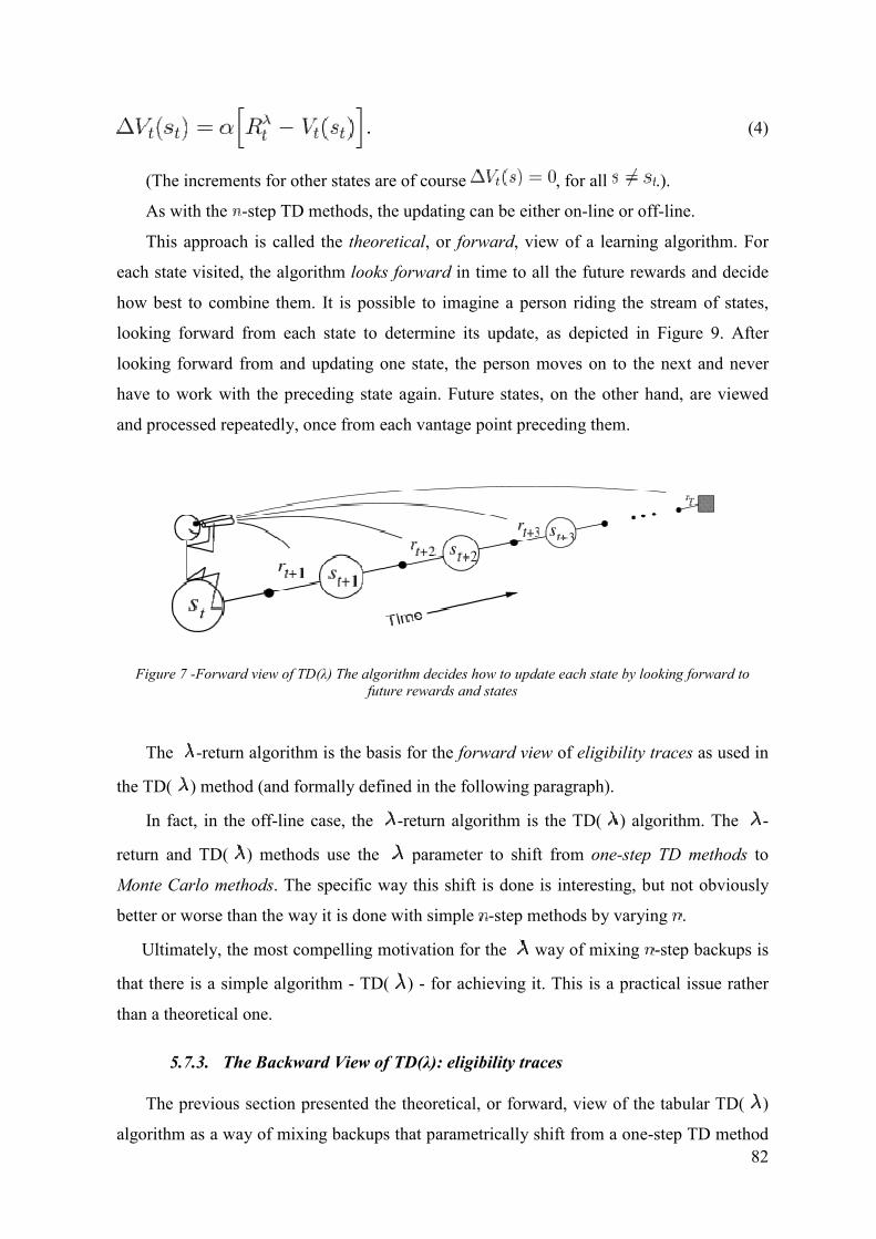
82

(4)

(The increments for other states are of course , for all .).

As with the -step TD methods, the updating can be either on-line or off-line.

This approach is called the theoretical, or forward, view of a learning algorithm. For

each state visited, the algorithm looks forward in time to all the future rewards and decide

how best to combine them. It is possible to imagine a person riding the stream of states,

looking forward from each state to determine its update, as depicted in Figure 9. After

looking forward from and updating one state, the person moves on to the next and never

have to work with the preceding state again. Future states, on the other hand, are viewed

and processed repeatedly, once from each vantage point preceding them.

Figure 7 -Forward view of TD(λ) The algorithm decides how to update each state by looking forward to

future rewards and states

The -return algorithm is the basis for the forward view of eligibility traces as used in

the TD( ) method (and formally defined in the following paragraph).

In fact, in the off-line case, the -return algorithm is the TD( ) algorithm. The -

return and TD( ) methods use the parameter to shift from one-step TD methods to

Monte Carlo methods. The specific way this shift is done is interesting, but not obviously

better or worse than the way it is done with simple -step methods by varying .

Ultimately, the most compelling motivation for the way of mixing -step backups is

that there is a simple algorithm - TD( ) - for achieving it. This is a practical issue rather

than a theoretical one.

5.7.3. The Backward View of TD(λ): eligibility traces

The previous section presented the theoretical, or forward, view of the tabular TD( )

algorithm as a way of mixing backups that parametrically shift from a one-step TD method

83

to a Monte Carlo method. This section instead defines TD( ) mechanistically, or

according a backward view: it is possible to proof that this mechanism correctly

implements the forward view. The mechanistic, or backward, view of TD( ) is useful

because it is simple both conceptually and computationally. In particular, the forward view

itself is not directly implementable because it is non-causal, using at each step knowledge

of what will happen many steps later. The backward view provides a causal, incremental

mechanism for approximating the forward view and, in the off-line case, for achieving it

exactly.

In the backward view of TD( ), there is an additional memory variable associated

with each state, its eligibility trace. The eligibility trace for state at time is denoted

. On each step, the eligibility traces for all states decay by , and the eligibility

trace for the one state visited on the step is incremented by :

(5)

for all non-terminal states , where is the discount rate and is the parameter

introduced in the previous section. Henceforth we refer to as the trace-decay parameter.

This kind of eligibility trace is called an accumulating trace because it accumulates each

time the state is visited, then fades away gradually when the state is not visited, as

illustrated below:

At any time, the traces record which states have recently been visited, where “recently”

is defined in terms of . The traces are said to indicate the degree to which each state is

eligible for undergoing learning changes should a reinforcing event occur. The reinforcing

events we are concerned with are the moment-by-moment one-step TD errors. For example,

the TD error for state-value prediction is

(6)

In the backward view of TD( ), the global TD error signal triggers proportional

updates to all recently visited states, as signalled by their nonzero traces:

84

(7)

As always, these increments could be done on each step to form an on-line algorithm,

or saved until the end of the episode to produce an off-line algorithm. In either case,

equations ((18)-(20)) provide the mechanistic definition of the TD( ) algorithm.

The backward view of TD( ) is oriented backward in time. At each moment we look

at the current TD error and assign it backward to each prior state according to the state’s

eligibility trace at that time. It is possible to imagine a person riding along the stream of

states, computing TD errors, and shouting them back to the previously visited states, as

suggested by Figure 11. Where the TD error and traces come together, we get the update

given by (20).

Figure 8- Backward view of TD(λ) - Each update depends on the current TD error combined with traces of

past events

To better understand the backward view, consider what happens at various values of

If , then by (18) all traces are zero at except for the trace corresponding to . In

terms of Figure 11, TD(0) is the case in which only the one state preceding the current one

is changed by the TD error. For larger values of , but still , more of the preceding

states are changed, but each more temporally distant state is changed less because its

eligibility trace is smaller, as suggested in the figure: it is possible to say that the earlier

states are given less credit for the TD error.

If , then the credit given to earlier states falls only by per step. This turns out to

be just the right thing to do to achieve Monte Carlo behaviour. For example, remember that

the TD error, , includes an undiscounted term of . In passing this back steps it needs

to be discounted, like any reward in a return, by , which is just what the falling eligibility

trace achieves. If and , then the eligibility traces do not decay at all with time.

85

In this case the method behaves like a Monte Carlo method for an undiscounted, episodic

task. If , the algorithm is also known as TD(1). TD(1) is a way of implementing

Monte Carlo algorithms.

Concluding, it is possible to proof that off-line TD( ), as defined mechanistically

above, achieves the same weight updates as the off-line -return algorithm: in this sense it

is possible align the forward (theoretical) and backward (mechanistic) views of TD( ).

Two different methods combining eligibility traces and Q-learning have been proposed

that sometimes these are referred as Watkins’s Q( ) and Peng’s Q( ), after the

researchers who first proposed them.

Let’s recall that Q-learning is an off-policy method, meaning that the policy learned

about need not be the same as the one used to select actions. In particular, Q-learning learns

about the greedy policy while it typically follows a policy involving exploratory actions -

occasional selections of actions that are suboptimal according to . Because of this, special

care is required when introducing eligibility traces.

Suppose to back up the state-action pair at time . Suppose that on the next two

time steps the agent selects the greedy action, but on the third, at time , the agent

selects an exploratory, non-greedy action. In learning about the value of the greedy policy

at it is possible to use subsequent experience only as long as the greedy policy is

being followed. Thus, it is possible to use the one-step and two-step returns, but not, in this

case, the three-step return. The -step returns for all no longer have any necessary

relationship to the greedy policy. Thus, unlike TD( ), Watkins’s Q( ) does not look

ahead all the way to the end of the episode in its backup. It only looks ahead as far as the

next exploratory action.

Aside for this difference, however, Watkins’s Q( ) is much like TD( ). Its look

ahead stops at episode’s end, whereas Q( )’s look ahead stops at the first exploratory

action, or at episode’s end if there are no exploratory actions before that.Actually, to be

more precise, one-step Q-learning and Watkins’s Q( ) both look one action past the first

exploration, using their knowledge of the action values.

The mechanistic or backward view of Watkins’s Q( ) is very simple. Eligibility traces

are just set to zero whenever an exploratory (non-greedy) action is taken. The trace update

is best thought of as occurring in two steps. First, the traces for all state-action pairs are

86

either decayed by or, if an exploratory action was taken, set to . Second, the trace

corresponding to the current state and action is incremented by .

The overall result is:

where, as before, is an identity indicator function, equal to 1 if and

otherwise.

The rest of the algorithm is defined by:

where

Unfortunately, cutting off traces every time an exploratory action is taken loses much

of the advantage of using eligibility traces. If exploratory actions are frequent, as they often

are early in learning, then only rarely will backups of more than one or two steps be done,

and learning may be little faster than one-step Q-learning. Peng’s Q( ) is an alternate

version of Q( ) meant to remedy this. Under specific conditions this method may

converge to , even if this has not yet been proved. Nevertheless, the method performs

well empirically. Most studies have shown it performing significantly better than Watkins’s

Q( ).

5.8. Learning and Planning methods

The term planning is used in several different ways in different fields. In particular, it

can be used to refer to any computational process that takes a model as input and produces

in output or improves a policy for interacting with the modelled environment.

A model of an environment can be defined as anything that an agent can use to predict

how the environment will respond to its actions: given a state and an action, the model

produces a prediction of the resultant next state and next reward. If the model is stochastic,

then there are several possible states and rewards, each with some probability of occurring.

Some models (called distribution models) produce a description of all the possible next

states and next rewards and their probability of occurring; other models (called sample

87

models) generate samples according to the (unknown) probability distribution. An example

of distribution model is that assumedin Dynamic Programming (based on the state

transition probabilities and expected rewards).

Within Artificial Intelligence there are two distinct approaches to planning according to

the above mentioned definition: state-space and plan-space planning..

In state-space approach, planning is viewed as a search through the state space for an

optimal policy or a path to a goal. Actions cause transitions from state to state and value

functions are computed over states.

In plan-space approach, planning is instead viewed as a search through the space of

plans. Operators transform one plan into another and value functions, if any, are defined

through the space of plans.

Referring to the state-space approach, it can be shown that there is a close

relationshipsbetween planning optimal behaviour and learning optimal behaviour, because

both processes involve estimating the same value functions. In fact, all state-space planning

methods involve computing value functions as a key intermediate step toward improving

the policy and compute their value functions by back-up operations applied to simulated

experience.

The main difference with learning methods (such as Temporal Difference methods) is

that whereas planning uses simulated experience generated by a model, learning methods

use real experience generated by the Environment.

Learning and planning processes can be easily integrated, allowing both to update the

same estimated value functions.

Moreover, all learning methods can be converted into planning methods, by applying

them to simulated (or model-generated) experience, rather than to real experience: in this

way, planning algorithms can be defined that are identical to learning algorithms but

operating on different sources of experience.

Finally, planning methods can be integrated with acting and model-learning. By model

learning we mean that when planning is done “on-line”, while interacting with the

environment, new information gained from the interaction with the environment may be

used to change (improve) the model and thereby interact with planning.

88

Examples of agents integrating planning and learning functionalities and able to “learn

a model” using real experience and to “learn optimal policies” using both real experience

(so-called “direct learning”) and simulated experience “(so-called “indirect learning”), are

known in literature as “Dyna agents”. In Dyna architecture, both direct and indirect

learning functions are achieved by applying Reinforcement Learning (typically Q-

Learning) algorithms.

89

6. THE PROPOSED RL APPROACH

This chapter illustrates the proposed RL approach for modelling and solving the QoE

problem addressed in this thesis work.

The first paragraph illustrates why the Reinforcement Learning approach was proposed,

considering several alternative approaches and methods developed in Control and Artificial

Intelligence fields.

The second paragraph illustrates why the Temporal Difference (TD) class of RL

algorithms and, in particular, why the Q-learning algorithm was selected.

The third paragraph illustrates some hybrid solutions combining Reinforcement

Learning and Games Theory (Learning in Games) and introducesan alternative RL

approach, based on the Friend or Foe algorithm. This approach seemspromising in term of

overcoming some limitations of the Q-Learning based solution when adopted in multi-agent

systems.

6.1. Why Reinforcement learning

Several alternative approaches and methods were investigated, in order to select the

most appropriate solution for solving the problem addressed in this thesis, considering, in

particular, theories and methods developed in the Control, Statistics and Artificial

Intelligence fields.

In particular, Optimal and Adaptive Control, Games Theory, Artificial Neural

Networks, Evolutionary/Genetic Algorithms and Planning methods were analyzed.

The choice of a Reinforcement Learning approach derived, first of all, from the

consideration that it seems natural and appropriate defining the QoE problem addressed in

this thesis like a “Reinforcement Learning Problem”, as illustrated in chapter 2.3: the

problem of implementing a Requirement Agent able to make, dynamically, an optimal

Class of Service choice, learning to make optimal decisions through direct experience in its

ICT Environment and with the goal of satisfying the Target Quality of Service of the

relevant Application without negatively impacting on the Global Quality of Service.

90

A second consideration drove the author to prefer a model-free approach, in order to

satisfy some of the main Future Internet Architecture requirements: flexibility and

independence from a specific technology and/or ICT domain or framework (to be known or

learned “a priori” and “off-line”).Consequently, robust, optimal and adaptivecontrol

methods were not selected because they are typically model-based.

Artificial Neural Networks typically follow a supervisedapproach, based on Training

examples (an external entity, the Supervisor, instructs the neural network on how to behave

in specific training situations) while, as said, the addressed problem requests a unsupervised

approach: the Requirement Agents must be able to learn from experience interacting with

the Environment. Supervised learning is associative but not selective, meaning that is

missing of the search (trial and selection of alternatives) component of trial and error

learning methods. The Reinforcement Learning methods are characterized by an

unsupervised approach because the RL agents learn through direct experience in interacting

with the environment, following a trial and error approach.

Natural selection in evolution is a prime example of a selective process, but is not

associative. Evolutionary/genetic algorithms were not selected because they are selective

but not associative: they do not use policies or associations between environment’s states

and agent’s actions and are not able to learn by interacting with the Environment.

Classic Artificial Intelligence Planning methods were not selected mainly because they

are based on prediction models that must be “learned” in some way: the Reinforcement

Learning approach seems more appropriate because it incorporates the learning function. It

should be observed that Reinforcement Learning Agents incorporate learning/prediction

and control functionalities and, when required, can be also efficiently integrated with

Planning functionalities (as illustrated in the previous chapter on Learning and Planning).

Multi-Agent System approaches based on consensus, cooperation ornegotiation

strategies were not adopted mainly because the need of cooperation and coordination

between Agents typically determinates strong real time communication requirements, either

between the Agents (in distributed models) or between the Agents and a centralized entity

(in centralized models): these requirements seem to be not sustainable in Future Internet

scenarios, particularly consideringInternet of Thing scenarios, where an increasing number

91

of “things” (objects or devices), with limited ICT and energy resources, shall be connected

to the Internet platform.

As a final consideration, it is important to underline that the choice of a Reinforcement

Learning approach for the reasons explained above doesn’t at all exclude the possibility of

combining Reinforcement Learning with other approaches, methods and algorithms in

order to better address, adopting hybrid solutions, specific problems that can arise when

adopting “pure” RL solutions in multi-agent systems.

In the last chapter, some hybrid solutions developed in Learning in Games theory and

combining Reinforcement Learning and Games Theory will be illustrated.One of those

solutions (Friend or Foe algorithm) seems promising in order to overcome some limitations

of the Q-Learning approach when adopted in multi-agent systems.

6.2. Why Q-Learning

As a first consideration, the choice of the specific RL algorithm for solving the problem

addressed in this thesis work and to be implemented in the considered scenarios was

strongly conditioned by the agents constraints: the agents have limited power and memory

capabilities and, consequently, the implementation of simple and efficient algorithms, with

a fast and simple learning processand a high speed of convergence to the optimal solution is

considered mandatory.

After an accurate comparison between features, advantages and disadvantages of the

three basic classes of RL methods as presented in the Chapter 5 (Dynamic Programming,

Monte Carlo methods and Temporal-Difference methods), an algorithm belonging to the

Temporal-Difference class was selected, for the reasons illustrated below.

As already said, Dynamic Programming methods are well developed mathematically,

but require strong assumptions: in particular, they require a complete and accurate model of

the environment as a Markov Process. Moreover, they requires a lot of computation time

and memory. For all these reasons, they were discarded.

Temporal-Difference methods in several aspects are similar to the Monte-Carlo

methods (in particular: they both do not require a model and operate performing sample-

92

backups on the states and samplings, meaning that the value function updates involve

estimations or expected value calculations) but, as said, they are fully step-by-step

incremental, while Monte Carlo methods are not suited for step-by-step incremental

computation. In Time Difference Methods the Agent learns at each step, while in Monte

Carlo methods it only learns at the end of each episode: the learning process in TD methods

is faster.

In addition, TD are “bootstrapping” methods, like DP ones. It should be noted that

bootstrapping methods are of persistent interest in Reinforcement Learning because, despite

some limited theoretical guarantees, in practice they usually work better than non-

bootstrapping methods.

On the other side, a disadvantage of bootstrapping methods is that they perform well

only in strictMarkov-tasks.When the tasks are at least partially non-Markov, than the use of

a pure Monte-Carlo method or of the eligibility traces (lambda-versions of TD algorithms)

is indicated, because eligibility traces can be considered the first “line of defense” against

non-Markov tasks (they do not bootstrap) and long-delayed rewards. It should be

considered that eligibility traces require more computation than one-step methods but, in

return, they offer faster learning, particularly when rewards are delayed by many steps.

In conclusion, assuming that our task is Markov and that rewards are not too long-

delayed, a simple, efficient, one-step TD algorithm, able to guarantee a high speed of

convergence to the optimal policy, was chosen: the off-policy Q-Learning algorithm.

6.3. An alternative proposal: the Friend or Foe algorithm

An interesting hybrid approach, combining Learning and Games Theory in multi-agent

system frameworks, is that proposed by the Learning in Games theory and, in particular, by

the so-called multi-player Stochastic Games.

The theory of Learning in Games studies the equilibrium concepts dictated by learning

mechanisms. That is, while the “classic” Nash equilibrium is based on the assumption of

“perfectly rational” players, in learning in games the assumption is that the agents use some

kind of learning algorithm. The theory determines the equilibrium strategy that will be

arrived at the various learning mechanisms and maps these equilibria to standard solution

concepts, if possible.

93

As far concerns the Stochastic Games, in many multi-agent applications the agents do

not know the future rewards they will receive for their actions. Instead, they must take

random actions in order to first explore the environment so that they may then determine

which actions lead them to the best future rewards starting from certain states. That is, the

agents live in a Markov chain and inhabit a multi-agentMarkov Decision Process (MDP).

As illustrated previously, the Reinforcement Learning is a very popular machine

learning approach to formally define (and solve) this kind of problem.The Reinforcement

Learning problem can be solved using several classes of methods and algorithms; as said,

one of the most widely used RL algorithms is the Q-Learning algorithm, that requires a

proper tuning of the learning rate α and of the exploration rate ε.

For the reasons illustrated in the previous chapter, a Q-Learning based approach has

been followed to solve the QoE problem addressed in this thesis work. Unfortunately, the

convergence properties of Q-Learning are impressive but they assume that only one agent

is learning and that the Environment is stationary.

When multiple agents are learning, the reward’s functions of each agent is no longer a

function of the state and the agent’s actions, but is a function of the state and all the agents’

actions. That is, each agent’s reward depends on the actions that other agents take, as

captured by the multi-agent MDP framework illustrated previously (Chapter 4).

In multi-agent MDPs, it might be impossible for a Q-learning agent to converge to an

optimal policy.

One possible solution to this problem is that of defining an hybrid solution combining

the advantages of the Reinforcement Learning approach with the equilibrium concept of

Games Theory.

In single agent problems, the target is defined in terms of finding an “optimal policy”,

that is maximizing the agent’s discounted future rewards.In multiple agent systems the

target could be defined in terms of maximising some global function of the agents’

discounted future rewards (for example their sum, as in the “social welfare” case) or,

alternatively, in terms of finding a particular equilibrium, more “interesting” from a

convergence point of view, such as the Nash Equilibrium Point (NEP).

A NEP is defined as a set of policies such that no one agent will gain anything by

changing its policy from its NEP strategies to something else.

94

As with the standard Nash equilibrium, it has been shown that a NPE always exists:

every n-player discounted stochastic game possesses at least one NEP in stationary

strategies.

In particular, a NEP can be found in a system where all the agents use a Nash Q-

Learning algorithm, that is a combination of a Q-learning algorithm and a Nash equilibrium

strategy. In this algorithm, each agent must keep n Q-tables, one for each agent in the

population. These tables are updated using a formula similar to the standard Q-Learning

one, but instead of using the Q-values to determine future rewards, it uses Nash Q-tables.

That is, at each step, the algorithm assumes that the multi-agent MDP game is defined

(induced) by the n Q-tables it has and then calculates a NEP for this problem. This can be

an extremely expensive computation, harder than finding the Nash equilibrium for a game

matrix.

The Nash Q-Learning algorithm is guaranteed to converge as long as enough time is

given so that all state-action pairs are explored sufficiently and if two assumptions hold: the

existence of an adversarial equilibrium and the existence of a coordination equilibrium for

the entire game and for each game defined by the Q functions encountered during learning.

An adversarial equilibrium is one where no agent has anything to lose if the other

agents change their policies from equilibrium, while a coordination equilibrium is one

where all the agents receive the highest possible value (that is the “social welfare

solution”).

These assumptions can be relaxed by assuming that each agent knows whether the

opponent is a “friend” (in this case a coordination equilibrium will be looked for) or a “foe”

(in this case an adversarial equilibrium will be looked for).

With this additional information, each agent no longer needs to maintain n Q tables

(one for each opponent) and can achieve convergence with only one, expanded, Q table.

The relevant algorithm is called the Friend or Foe Q-Learning algorithm.

This algorithm implements the idea that, for each agent i, i’s friends are assumed to

work together to maximize i’s value while i’s foes work together to minimize i’s value.

This algorithm always converges to a stable policy and converges to a NEP under the

assumption that the game has an adversarial equilibrium or a coordination equilibrium.

Friend or Foe algorithm has several advantages over Nash Q-Learning. It does not

require the learning of n Q functions (one for each one of the other agents) and it is easy to

implement because it does not require the calculation of a NEP at each step. On the other

95

hand, it does require to know if the opponents are friends or foes, that is whether exists a

coordination or an adversarial equilibrium.

Neither algorithm deals with the problem of finding equilibria in cases without either

coordination or adversarial equilibria: such cases are very common and require some degree

of cooperation among otherwise selfish agents.

The theory of learning in games provides the designers of multi-agent systems with

many useful tools for determining the possible equilibrium points of a system.

However, it is important to underline that, in general, the designers of multi-agent

systems are not able to predict which equilibria, if any, the system will converge to (which

“equilibrium solution” will emerge): this fact is due to two main reasons: the existence of

unpredictable environmental changes that can affect the agents rewards and the fact that in

many systems each agent has not access to other agents’ rewards.

Learning agents are often used by system designers, but, in general, changes in the

design of the system and learning algorithms affect time of convergence.

One problem with learning agents is that, as the agents change their behaviour, in a

continuous effort to maximize their utility, the rewards for their actions will change,

changing their expected utility. The system will likely have non stationary dynamics,

because it will be always changing to match the new goal. While games theory indicates

where the equilibrium points are (given that rewards stay fixed), multi-agent systems often

never “get” to those (moving) points.

96

7. COGNITIVE APPLICATION INTERFACE: THE PROPOSED RL

FRAMEWORK

The proposed Cognitive Application Interface is based on a Reinforcement

Learningframework.

For the reasons illustrated in the previous chapter, the QoE problem addressed by the

Application Interface can be modelled as a Reinforcement Learning problem, where the RL

Agent role is played by the Requirement Agent.

The Requirement Agent must be able to learn to make optimal decisions based on

experience with anEnvironment,to bemodelled with an appropriate state space and reward

function, as illustrated in this chapter.

7.1. Supervisor Agent

At each time tlthe Supervisor Agent computes, for each Service Class k (from 1 to K), a

set of parameters ΘSA(tl,k). The parameters ΘSA(tl,k) are computed by the Supervisor Agents

by exploiting measurements taken in the time interval [tl−Tmonit-l, tl], where Tmonit-lis a proper

monitoring period.

In order to take these measurements, the Supervisor Agent can either directly monitor

the traffic relevant to the in-progress applications, or set-up a few probe applications (i.e.

not corresponding to applications set-up by the Actors) statically associated to the Service

Classes k (from 1 to K). The most appropriate implementation has to be tailored to the

reference scenario.

At each time tl the Supervisor Agent broadcasts the monitored parameters ΘSA(tl,k) (for

k=1,…,K) to all the Requirement Agents. These parameters are included in proper signaling

messages, hereinafter referred to as Status Signals and indicated as ss(tl), where:

ss(tl) = [ ΘSA(tl,1), ΘSA(tl,2),…, ΘSA(tl,K)]

The signalling overhead introduced by the Status Signal consists in broadcasting LK

bits, where L is the number of bits necessary to code ΘSA(tl,k) and K is the total number of

Service Classes, every Tlseconds, where Tl is the duration of the period between the

broadcast of a given status signal and the next one, i.e. Tl=tl+1-tl. Indeed, this seems to be a

very reasonable signalling overhead, even considering that we are referring to a broadcast

97

signal (sent from the single Supervisor Agent to the many Requirement Agents) and no

signalling is foreseen in the opposite direction (i.e. from the Requirement Agents to the

Supervisor Agent).

According to this proposal, the information deduced from the Status Signal which fed

the Requirement Agent in Fig. 3, are just the parameters ΘSA(tl,k), k=1,…,K.

7.2. Requirement Agent

The issues of this section applies to any Requirement Agent. Then, without loss of

generality, let us consider a given Requirement Agent a, namely the one relevant to the

Application a.

At each time tsthe Requirement Agent a receives from the Elaboration functionalities a

set of feedback parametersΘ(ts,a) referring to the application a.The parameters Θ(ts,a) are

computed by the Elaboration and Sensing functionalities by exploiting measurements taken

in the time interval [ts−Tmonit-s, ts], where Tmonit-sis a proper monitoring period.

The Requirement Agent a receives from the Application Handler a a function ha which,

at each time ts, allows to compute the Measured QoE(QoEmeas(ts,a)) on the basis of the

feedback parameters Θ(ts,a), i.e.

QoEmeas(ts,a) = ha(Θ(ts,a)). (7.1)

Moreover, at each time tl, the Requirement Agent a receives the Status Signal ss(tl) and

hence the parameters ΘSA(tl,k) (k=1,…,K). The parameters Θ(ts,k) should have the same

nature as the parameters ΘSA(tl,a), so that the Requirement Agent a, by using the function

ha, can compute the so-called QoE relevant to the Service Class k (from 1 to K), hereinafter

indicated as QoE(tl,a,k), in the following way:

QoE(tl,a,k) = ha(ΘSA(tl,k)) with k=1,…,K (7.2)

The global information contained in the parameters QoE(tl,a,k) (k=1,…,K) provides an

estimate of the general network state, by Service Class, analysed from the perspective of the

Requirement Agent a (since the personalized function ha is used for the computation of

these parameters).

98

The parameter QoE(tl,a,k) represents an estimate of the QoE that the application a will

experience at times tsnext to tlif the Requirement Agent a selects the Service Class k. Such

parameter is an estimate both because tsis next to tl and because the Supervisor Agent has a

different perspective (as concerns parameters to be monitored) than the Requirement Agent

a. Nevertheless, even though the parameters QoE(tl,a,k) are estimates, they seem

appropriate in order to provide the Requirement Agent a with a rough preview of what is

going to happen if the Requirement Agent will select, in the near future, the Service Class

k. In this respect, note that the parameters QoE(tl,a,k) take into account the personalized

way of the application a, to assess its own QoE, since such way is embedded in the function

ha.

On the basis of the above-mentioned information (QoEmeas(ts,a)and QoE(tl,a,k), k=1,..,

K), the Requirement Agent a has the key role of selecting, at each time ts, the most

appropriate Class of Service k(ts,a) to be associated to the micro-flow supporting the

Application a, aiming at the target Application QoE mentioned in chapter3.2.

In order to perform the above-mentioned very critical selection, the Requirement Agent

is provided with a Reinforcement Learning algorithm, as detailed in the next paragraph.

7.3. The Reinforcement Learning problem

The main elements of the considered Reinforcement Learning problem (state space,

action space and reward function) are defined as follows.

The action that the Requirement Agent a has to perform is to select,at each time ts, the

proper Service Class k(ts,a). The action space dimension is equal to K (number of Service

Classes).

As far concerns thestate variables, a suitable selection, at time

ts,includesQoEmeas(ts,a),QoE(tl,a,1),QoE(tl,a,2),…,QoE(tl,a,K), possibly normalized with

respect to QoEtargetand quantized.

The state space dimension is N^K+1

, where K is the number of Classes of Service and N

is the number of possible QoE levels: in order to keep the state space dimension limited, N

should be carefully defined. Consequently, the state-action value matrix Q has dimension

equal to N^K+1

x K.

99

In this way, the Reinforcement Learning algorithm of the Requirement Agent a is

provided with a suitable information set including:

(i) local information contained in the parameter QoEmeas(ts,a) reflecting the local

situation taking place at the Requirement Agent a,

(ii) global information contained in the parameters QoE(tl,a,k) (k=1,…,K) providing an

estimate of the general network state analysed from the perspective of the

Requirement Agent a (since the personalized function ha is used for the

computation of these parameters).

Finally, as far concerns thereward functionr(ts), a promising choice is the following:

r(ts) = − [QoEmeas(ts,a)−QoEtarget(a)]2

=-e(ts,a) 2

By adopting this function, whenever the measured QoE is different from the target QoE

the reward is negative (that is, the agent is punished), and is equal to zero only when

QoEmeas(ts,a) =QoEtarget(a). In this way, we push the Requirement Agent to drive the

Service Class selection so that the Measured QoE approaches the Target QoE.

A possible alternative reward function is the following:

r(ts) = − [QoEmeas(ts,a) −QoEtarget(a)]2

if QoEmeas(ts,a) <QoEtarget(a);

r(ts) = 0 if QoEmeas(ts,a) >QoEtarget(a).

This reward function differs from the previous one if QoEmeas(ts,a) >QoEtarget(a); in this

case the reward is zero, i.e. we do not penalize nor award the Requirement Agent for

achieving a Measured QoE higher than the Target QoE.

The rationale behind this difference lies in the fact that if the application relevant to a

given Requirement Agent overperforms, consuming resources at the expenses of the

applications relevant to other Requirement Agents (that underperform), the reward function

of these last Requirement Agents should drive the overall system to move resources from

the Requirement Agent a to the other Requirement Agents; otherwise, the RA can continue

to use the available resources.

100

8. COGNITIVE APPLICATION INTERFACE: THE QOS CASE

In this and in the following chapters the concepts introduced so far will be

particularized to the Quality of Service of in progress Applications.

Nevertheless, it is worth stressing again that all the concepts introduced so far can also

be applied to all other issues which impact on the QoE (e.g. security, mobility, contents,

etc.); as a matter of fact, in order to include even these other issues, it is sufficient to

properly define the relevant metrics and requirements and the personalized QoE function ha

allowing to measure the QoE of the Application a as a function of the parameters

considered in the metrics in question.

8.1. QoS Metrics and Requirements

The proposed QoS Metric is based on the following QoS Service Class Parameters:

- D(f,t): Transfer delay (sec) for the traffic relevant to the flow f at time t is the average

delay experienced by its packets from the time they entered the network to the time t

when they arrive to the outgoing node.

- Radm(f,t): Admitted bit rate (bps) for the traffic relevant to the flow f at time t is the bit

rate of traffic to be carried by the network.

- L(f,t): Loss Rate(bps) for the traffic relevant to the flow f at time t is the traffic lost in

the network (due to possible drops, caused by congestion/overflow, or errors, caused

by the physical link techniques).

Each QoS Service Classk makes reference to the following QoS Service

ClassReference Values:

- Dmax(k): Maximum transfer delay (sec)

- Radm-min(k): Minimum guaranteed (committed)bit rate (bps);

- Lmax(k): Maximum Loss Rate (bps);

Taking into account the introduced Service Class Parameters, for a Service Class k, the

associatedQoS Service Class Requirements, for each monitoring period, are the following:

D(f,t) <Dmax(k) (8.1)

Radm(f,t) >Radm-min(f) (8.2)

101

L(f,t) <Lmax(f) (8.3)

The task of the Elaboration functionalities in the Cognitive Managers is to control the

Resource exploitation of the network so that for every Service Class, the previous

inequalities are, as far as possible, simultaneously satisfied.

8.2. Cognitive Application Interface: an example with QoS

As it has already been stressed in Chapter 3, the number of QoE/QoS Service Classes is

a limited and hence, in general, the QoE/QoS Requirements of a given Application do not

match with any predefined Service Class Requirements.

So, referring to the QoS Metric introduced in the previous paragraph, in general, the

personalized QoE/QoS Requirements of a given Application a make reference to the

following QoE/QoSApplication Reference Values:

- Dmax(a): Maximum transfer delay (sec)

- Radm-min(a): Minimum guaranteed bit rate (bps);

- Lmax(a): Maximum Loss Rate (bps);

- QoEtarget(a): Target reference QoE level.

As for the personalized function ha allowing the computation of the QoE experienced

by the Application a(rif. Chapter 7.2),two options are suggested.

- Afirst considered option is to identify QoEmeas(ts,a) with the Link AvailabilityLA(a,ts)

of the Application a, defined as the percentage of time, computed over the time interval

[t0, ts], in which the following inequalities are simultaneously met:

D(a,t) <Dmax(a)

Radm(a,t) >Radm-min(a)

L(a,t) <Lmax(a)

where the parameters D(a,t), Radm(a,t) and L(a,t) refer to the micro-flow supporting

the Application a. In this case the personalized function ha can be identified with a very

simple algorithm which, on the basis of (i) the values assumed by the parameters D(a,t),

Radm(a,t) and L(a,t) in the time interval [t0, ts] and (ii) the QoSApplication Reference

102

Values Dmax(a), Radm-min(a) and Lmax(a), computes the corresponding Link Availability

LA(a,ts).

- Asecond considered option is the following weighted QoE function:

QoEmeas(ts,a) = α1 min[1, 1 − (Radm-min(a)−Radm(a,ts))/ Radm-min(a)] +

α2 min[1, 1 − (D(a,ts)−Dmax(a))/ Dmax(a)] +

α3 min[1, 1 − (L(a,ts)−Lmax(a))/ Lmax(a)]

where α1, α2, α3 are three constants in the range [0,1],subject to the

constraintα1+ α2+ α3=1,to be selected according to the relative importance granted to

admitted bit rate, delays and los rate.

The second function allows to define in a smoother and more granular way the global

quality actually perceived by the Actors, considering the QoS degradationlevelassociated to

each QoS parameter and weighting each QoS parameter according to its relative

importance.

8.2.1. Supervisor Agent in the QoS case.

In this section we will particularize to the QoS case what has been presented, in the

general case, in chapter 7.1.

At each time tlthe Supervisor Agent computes, for each Service Class k (from 1 to K),

the following set of parameters ΘSA(tl,k):

ΘSA(tl,k) = [Dmeas-SA(tl,k), Lmeas-SA(tl,k), Radm-meas-SA(tl,k)]

where Dmeas-SA(tl,k), Lmeas-SA(tl,k), Radm-meas-SA(tl,k)are measurements referring to the

parameters introduced in Section 6.1, taken by the Supervisor Agent in the time interval

[tl−Tmonit-l, tl], where Tmonit-lis a proper monitoring period, and referring to the various

Service Classes k(from 1 to K).

At each time tl, the Supervisor Agent broadcasts to all the Requirement Agents the

following Status Signalss(tl):

ss(tl) = [ΘSA(tl,1), ΘSA(tl,2),…, ΘSA(tl,K)]

103

8.2.2. Requirement Agent in the QoS case

In this section we will particularize to the QoS case what has been presented, in the

general case, in chapter 7.2.

Without loss of generality, let’s consider a given Requirement Agent a, namely the one

relevant to the Application a.

At each time ts,the Requirement Agent a receives from the Elaboration

functionalitiesthe following set of parameters Θ(ts,a) referring to the Application a:

Θ(ts,a) = [Dmeas(ts,a), Lmeas(ts,a), Radm-meas(ts,a)]

where Dmeas(ts,a), Lmeas(ts,a), Radm-meas(ts,a)are measurements referring to the parameters

introduced in the section 6.1, taken by the Requirement Agent in the time interval

[ts−Tmonit-s, ts], where Tmonit-sis a proper monitoring period.

Then, at each time ts, on the basis of these parameters and of the function ha, the

Requirement Agent a can compute the Measured QoEQoEmeas(ts,a), as defined in chapter

7.2 (formula 7.1).

Moreover, at each time tl, the Requirement Agent receives the Status Signal and, on the

basis of the relevant parameters and of the function ha, can compute the QoE relevant to the

Service Class kQoE(tl,a,k) (from 1 to K), as defined in chapter 7.1 (formula 7.2).

On the basis of the above-mentioned information, the Requirement Agent a has the key

role of selecting, at each time ts, the most appropriate Service Class k(ts,a) to be associated

to the micro-flow supporting the Application a. In order to perform the above-mentioned

critical selection, the Requirement Agent is provided with a Reinforcement Learning

algorithm.

The state variables, the action and the reward function characterizing the

Reinforcement Learning problem are those defined in chapter 7.3.

104

9. REAL NETWORK SCENARIOS

In this chapter we focus on possible real network scenarios in which the approach

presented in this thesis can be adopted.

Referring to the QoS case, we are going to examine the case of access networks (both

in the wired and wireless scenario), since these type of networks are in general

characterized by limited bandwidth capability, an issue that is particularly critical from the

QoS point of view. The access networks can be considered as the actual bottleneck of the

end-to-end connectivity from the QoS point of view, whilst the core network can be

assumed as overprovisioned from the bandwidth point of view, that means that it does not

introduce meaningful delays, losses, or throughput limitations, and hence not actually

impacting on the QoS.

So, in the following, we deal with the fixed, cellular and ad-hoc access network cases,

focusing on the physical positioning of the Application Handler, Supervisor Agent and

Requirement Agent within the Cognitive Managers embedded in the various network

entities.

9.1. Fixed Networks

A fixed access network is composed by several fixed terminals, connected to the core

network by means of a Gateway.

Downlink side (from the Gateway to the fixed terminals)

This is the case occurring whenever a fixed user triggers an application entailing a

download (e.g. of a video file) from the network up to the fixed terminal.

In this case, the Application Handler has to be placed in the Cognitive Manager

embedded in the fixed terminal running the application in question. By so-doing the

Application Handler can easily interact with the Application protocols and with the user, in

order to deduce the parameter QoEtarget, as well as the function h for QoE computation.

According to the concept sketched in Fig. 3, QoEtarget and h have to be sent to the

Requirement Agent (see Fig. 9). This figure refers to the case in which three Applications

105

(with the corresponding three Requirement Agents (RAs)) involving three different Fixed

Terminals are present.

Gateway

S

A

R

A

A

H

S

A

Requirement

Agent

Application

Handler

Supervisor

Agent

Wired

LinkFixed Terminal 1

AH

1

Core

Network

Queuing

Processes

Fixed Terminal 2

Fixed Terminal 3

RA

1

RA

2

AH

2

AH

3

RA

3

Figure 9 - Application Interface Architecture:-Fixed network - Downlink Side

The Requirement Agent has to be placed in the Cognitive Manager of the Gateway

since this last is in a position suitable for assessing the performance parameters D, Radm,

BER of the considered application, which can be easily deduced by monitoring the queues

in which the packets relevant to the application in question are temporary stored waiting for

being transmitted over the wired link. In Figure 9 the queues monitored by Requirement

Agents are depicted: each of these queues is associated to a specific Service Class and

stores the packets relevant to the associated Service Class (in the previous example we

assume there are four possible Classes of Service).

Note that, in this particular case, the Requirement Agents relevant to applications

running in fixed terminals served by a same Gateway are all placed in the Gateway itself.

So a cooperative approach would be possible, likely yielding to better performance than the

adopted non cooperative Q-learning algorithm.

As far as the Supervisor Agent is concerned, it is in charge of obtaining global

information on the network, and for this reason we identify its natural position inside the

Cognitive Manager of the Gateway. In order to compute the parameters ΘSA(tl,k) (necessary

for generating the Status Signal to be transmitted to the Requirement Agents) for each Class

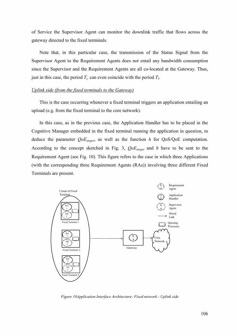
106

of Service the Supervisor Agent can monitor the downlink traffic that flows across the

gateway directed to the fixed terminals.

Note that, in this particular case, the transmission of the Status Signal from the

Supervisor Agent to the Requirement Agents does not entail any bandwidth consumption

since the Supervisor and the Requirement Agents are all co-located at the Gateway. Thus,

just in this case, the period Ts can even coincide with the period Tl.

Uplink side (from the fixed terminals to the Gateway)

This is the case occurring whenever a fixed terminal triggers an application entailing an

upload (e.g. from the fixed terminal to the core network).

In this case, as in the previous case, the Application Handler has to be placed in the

Cognitive Manager embedded in the fixed terminal running the application in question, to

deduce the parameter QoEtarget, as well as the function h for QoS/QoE computation.

According to the concept sketched in Fig. 3, QoEtarget and h have to be sent to the

Requirement Agent (see Fig. 10). This figure refers to the case in which three Applications

(with the corresponding three Requirement Agents (RAs)) involving three different Fixed

Terminals are present.

Gateway

S

A

R

A

A

H

S

A

Requirement

Agent

Application

Handler

Supervisor

Agent

Wired

Link

Fixed Terminal 1

RA

1

Fixed Terminal 2

Fixed Terminal 3

Queuing

Processes

Cloud of Fixed

Terminal

Core

Network

AH

1

RA

2

AH

2

RA

3

AH

3

Figure 10Application Interface Architecture: Fixed network - Uplink side

107

The Requirement Agent has to be placed in the Cognitive Manager of the Fixed

Terminal since this last is in a position suitable for assessing the performance parameters D,

Radm, BER of the considered application, which can be easily deduced by monitoring the

queues in which the packets relevant to the application on question are temporary stored

waiting for being transmitted over the wired link. Note that, in this case, the Requirement

Agents relevant to applications running in different fixed terminals are all placed in

different physical position. So, such Requirements Agents could not exchange information

one another, thus justifying the adopted non cooperative Q-learning algorithm.

As far as the Supervisor Agent is concerned, similar considerations apply as the ones

described in the previous section. Just note that, in this particular case, the transmission of

the Status Signal from the Supervisor Agent to the Requirement Agents entails bandwidth

consumption since the Supervisor and the Requirement Agents are all located at the

Gateway and at the Fixed Terminals respectively. A possible way, in order to limit such a

consumption, is to select the period Tl much longer than the period Ts.

9.2. Mobile Networks

9.2.1. Cellular Network

Downlink side (from the Base Station to the mobiles)

This is the case occurring whenever a mobile user triggers an application entailing a

download (e.g. of a video file) from the network up to the mobile terminal.

In this case, the Application Handler has to be placed in the Cognitive Manager

embedded in the mobile terminal running the application in question to deduce the

parameter QoEtarget, as well as the function h for QoE computation. Hence, these values

have to be sent to the Requirement Agent (see Figure 11). This figure refers to the case in

which three Applications (with the corresponding three Requirement Agents (RAs))

involving three different Mobile Terminals are present.

108

Mobile Terminal 1

Base

Station

S

A

RA

1

AH

1

R

A

A

H

S

A

Requirement

Agent

Application

Handler

Supervisor

Agent

Wireless

Link

Mobile Terminal 2 Mobile Terminal 3

Queuing

Processes

Core Network

AH

2

AH

3

RA

2

RA

3

Figure 11- Application Interface Architecture: Cellular Network - Downlink Side

The Requirement Agent has to be placed in the Cognitive Manager of the Base Station

since this last is in a position suitable for assessing the performance parameters D, Radm,

BER of the considered application, which can be easily deduced by monitoring the queues

in which the packets relevant to the application on question are temporary stored waiting

for being transmitted over the air interface. In Figure 11 the queues monitored by

Requirement Agents are depicted: each of these queues is associated to a specific Service

Class and stores the packets relevant to the associated Service Class (in the previous

example we assume there are four possible Class of Service).

Note that, in this particular case, the Requirement Agents relevant to applications

running in mobile served by a same Base Station are all placed in the Base Station itself.

So, such Requirements Agents could exchange information one another without introducing

signalling overhead: this means that, just in this particular case, a cooperative approach

would be possible, likely yielding to better performance than the adopted non cooperative

Q-learning algorithm. Nevertheless, the approach proposed in this thesis has the major

advantage of being applicable even in all scenarios (e.g. see in the following) in which an

heavy signalling exchange (as it would be required in a cooperative case) among

Requirement Agents is not feasible or efficient. .

109

As far as the Supervisor Agent is concerned, it is in charge of obtaining global

information on the network, and for this reason we identify its natural position inside the

Cognitive Manager of the Base Station. In order to compute the parameters

ΘSA(tl,k) (necessary for generating the Status Signal to be transmitted to the Requirement

Agents) for each Class of Service the supervisor Agent can: (i) monitor the downlink traffic

that flows across the base station directed to the mobile terminals relevant to in progress

applications triggered by the mobile terminals, and/or (ii) monitor the downlink traffic

relevant to so-called probe applications, i.e. fake applications, set by the Supervisor Agent

with dummy mobiles (i.e. with mobile terminals placed at a convenient distance of the Base

Station and handled by the network operator) just with the aim to measure the parameters

ΘSA(tl,k).

Note that, in this particular case, the transmission of the Status Signal from the

Supervisor Agent to the Requirement Agents do not entail any bandwidth consumption

since the Supervisor and the Requirement Agents are all co-located at the Base Station.

Thus, just in this case, the period Ts can even coincide with the period Tl.

Uplink side (from the mobiles to the Base Station)

This is the case occurring whenever a mobile user triggers an application entailing an

upload (e.g. from the mobile terminal to the fixed network).

In this case, as in the previous case, the Application Handler has to be placed in the

Cognitive Manager embedded in the mobile terminal running the application in question.

By so-doing the Application handler can easily interact with the Application Protocols and

with the user, in order to deduce the parameter QoEtarget, as well as the function h for

QoS/QoE computation. According to the concept sketched in Fig. 3, QoEtarget and h have to

be sent to the Requirement Agent (see Fig. 12). This figure refers to the case in which three

Applications (with the corresponding three Requirement Agents (RAs)) involving three

different Fixed Terminals are present.

110

Mobile Terminal 1 Mobile Terminal 2 Mobile Terminal 3

Base

StationS

A

RA

1

R

A

A

H

S

A

Requirement

Agent

Application

Handler

Supervisor

Agent

Wireless

Link

Queuing

Processes

Core Network

AH

1

RA

2

AH

2

RA

3

AH

3

Figure 12 - Application Interface Architecture: Cellular network -Uplink Side

The Requirement Agent has to be placed in the Cognitive Manager of the Mobile

Terminal since this last is in a position suitable for assessing the performance parameters D,

Radm, BER of the considered application, which can be easily deduced by monitoring the

queues in which the packets relevant to the application on question are temporary stored

waiting for being transmitted over the air interface. Note that, in this case, the Requirement

Agents relevant to applications running in different mobiles are all placed in different

physical position. So, such Requirements Agents could not exchange information one

another, thus justifying the adopted non cooperative Q-learning algorithm.

As far as the Supervisor Agent is concerned, similar considerations apply as the ones

described in the previous section. Jus note that, in this particular case, the transmission of

the Status Signal from the Supervisor Agent to the Requirement Agents entail bandwidth

consumption since the Supervisor and the Requirement Agents are all located at the Base

Station and at the Mobile Stations respectively. So, in order to limit such a consumption,

motivates the period Tl has to be selected much longer than the period Tl.

111

9.2.2. Ad-hoc Network

In ad-hoc networks, differently from cellular networks, direct mobile-to-mobile

communication can be admitted. So, mobiles can communicate one another either directly

(i.e. in a single-hop fashion) if they are in mutual visibility, or exploiting other mobiles as

communication bridges (i.e. in a multi-hop fashion); in addition, at least one mobile in the

network is provided with the so-called gateway functionalities, i.e. it can be connected with

the outside world. Usually, the ad-hoc mobiles self-organize themselves in clusters where

each cluster dynamically elects a cluster coordinator mobile which is usually dynamically

selected as the mobile located in the position closest to the cluster baricenter (from the

radio-electrical point of view) (see Fig. 13). Note that all mobiles are provided with the

cluster coordination functionalities since they are all potentially eligible as cluster

coordinators.

R

A

A

H

S

A

Requirement

Agent

Application

Handler

Supervisor

Agent

Wireless

Link

Queuing

Processes

Mobile Terminal 2

Mobile Terminal 1

RA

1

Coordinator

Mobile Terminal

R

A

A

H

Mobile Terminal 3

Mobile Terminal 4

S

A

AH

1

RA

2

AH

2

RA

3

AH

3

RA

4

AH

4

Figure 13 - Application Interface Architecture: Ad-hoc network

In this scenario the Application Handler has to be placed in the Cognitive Manager

embedded in the mobile terminal triggering the application in question, for the same

reasons as the ones exposed for the cellular network scenario. In addition, a Requirement

Agent has to be placed in the Cognitive Manager of each mobile terminal in charge of

transmitting the traffic coming from or directed to the mobile triggering the application,

112

again for the same reasons as the ones exposed for the cellular network scenario (see Fig.

8). Note that, in the multi-hop case, the Application Handler has to carefully select the

QoEtarget to be assigned to the various Requirement Agents embedded in the mobiles

involved in the multi-hop transmission, since the composition of the QoEtarget imposed to

the single hops have to generate the QoEtarget associated to the multi-hop. Note that, once

these assignments have been performed each hop can evolve independently of one another.

As far as the Supervisor Agent is concerned, it can be conveniently placed in the

Cognitive Manager of the cluster coordinator mobile since this last, by definition, due to its

baricentral position within the cluster, has the best vision of the present performance

occurring within the cluster.

113

10. IMPLEMENTED NETWORK SCENARIO

This chapter illustrates the adopted simulation tool (OPNET) and the implemented

Model Specification, describing the Network Model, the QoS policy and the Requirement

and Supervisor Agent algorithms.

10.1. Simulation tool: OPNET

Originally developed at MIT, OPNET (Optimized Network Engineering Tools)

Modeller has been introduced in 1987 as the first commercial network simulation tool and

actually provides a comprehensive development environment supporting the modelling of

communication networks and distributed systems.

Both behaviour and performance of modelled systems can be analysed by performing

discrete event simulations; it’s worth highlighting that the OPNET environment

incorporates editors and tools for all phases of a study, including model design, simulation,

data collection and data analysis. This paragraph, which aims at providing an overview of

OPNET capabilities and structure, is divided into the following four sub-sections:

• Key System Features: enumerates salient and distinctive characteristics of the

OPNET software;

• Typical Applications: presents some applications typically addressed with OPNET

and some of the features that provide direct support for those applications;

• Modelling Methodology: describes the OPNET approach to each phase of the

modelling and simulation project and presents fundamental modelling constructs;

• Editors and Tools: introduces the editors and tools that constitute the OPNET

environment; each editor, as far as each generic tool, supports a particular phase or

sub-phase of the simulation and modelling project.

10.1.1. Key System Features

OPNET is a vast software package with an extensive set of features designed to support

general network modelling and to provide specific support for particular types of network

simulation projects. This section aims at providing a brief enumeration of some of the most

important OPNET capabilities:

114

• Object orientation: systems specified in OPNET consist of objects, each with

configurable sets of attributes. Objects belong to “classes” which provide them with

their characteristics in terms of behaviour and capability. Definitions of new classes

are supported in order to address as wide a scope of systems as possible. Classes can

also be derived from other classes, or “specialized” in order to provide more specific

support for particular applications;

• Specialized in communication networks and information systems: OPNET provides

many constructs relating to communications and information processing, ensuring

high leverage for modelling of networks and distributed systems;

• Hierarchical models: OPNET models are hierarchical, naturally paralleling the

structure of actual communication networks;

• Graphical specification: wherever possible, models are entered via graphical

editors. These editors provide an intuitive mapping from the modelled system to the

OPNET model specification;

• Flexibility to develop detailed custom models: OPNET provides a flexible, high-

level programming language with extensive support for communications and

distributed systems. This environment allows realistic modelling of all algorithms,

communications protocols and transmission technologies;

• Automatic generation of simulations: model specifications are automatically

compiled into executable, efficient, discrete-event simulations implemented in the C

programming language. Advanced simulation construction and configuration

techniques minimize compilation requirements;

• Application-specific statistics: OPNET provides numerous built-in performance

statistics that can be automatically collected during simulations. In addition,

modellers can augment this set with new application-specific statistics that are

computed by user-defined processes;

• Integrated post-simulation analysis tools: performance evaluation and trade-off

analysis require large volumes of simulation results to be interpreted. OPNET

includes a sophisticated tool for graphical presentation and processing of simulation

output;

115

• Interactive analysis: all OPNET simulations automatically incorporate support for

analysis via a sophisticated interactive “debugger”;

• Animation: simulation runs can be configured in order to automatically generate

animations of the modelled system at various levels of detail and can include

animation of statistics as they change over time. Extensive support for developing

customized animations is also provided;

• Application program interface (API): as an alternative to graphical specification,

OPNET models and data files may be specified via a programmatic interface. This

is useful for automatic generation of models or to allow OPNET to be tightly

integrated with other tools.

10.1.2. Typical Applications

As a result of the capabilities that were described in the previous sections, OPNET can

be used as a platform to develop models of a wide range of systems. Some examples of

possible applications are listed below:

• Standards-based LAN and WAN performance modelling: detailed library models

provide major local-area and wide-area network protocols. The library also provides

configurable application models, or new ones can be created;

• Inter-network planning: hierarchical topology definitions allow arbitrarily deep

nesting of sub-networks and nodes and large networks are efficiently modelled;

scalable, stochastic and/or deterministic models can also be used in order to generate

network traffic;

• Research and development in communications architectures and protocols: OPNET

allows specification of fully general logic and provides extensive support for

communications-related applications. Finite state machines provide a natural

representation for protocols;

• Distributed sensor and control networks, “on-board” systems: OPNET allows

development of sophisticated, adaptive, application-level models, as well as

underlying communications protocols and links. Customized performance metrics

can be computed and recorded, scripted and/or stochastic inputs can be used to drive

116

the simulation model, and processes can dynamically monitor the state of objects in

the system via formal interfaces provided by statistic wires;

• Resource sizing: accurate, detailed modelling of a resource’s request-processing

policies is required to provide precise estimates of its performance when subjected

to peak demand (for example, a packet switch’s processing delay can depend on the

specific contents and type of each packet as well as its order of arrival). Queuing

capabilities of Proto-C provide easy-to-use commands for modelling sophisticated

queuing and service policies; library models are provided for many standard

resource types;

• Mobile packet radio networks: specific support for mobile nodes, including

predefined or adaptive trajectories; predefined and fully customisable radio link

models; geographical context provided by OPNET network specification

environment.(Radio version only);

• Satellite networks: specific support for satellite nodes, including automatic

placement on specified orbits, a utility program for orbit generation and

visualization and, finally, an orbital configuration animation program. (Radio

version only);

• C3I and tactical networks: support for diverse link technologies; modelling of

adaptive protocols and algorithms in Proto-C; notification of network component

outages and recoveries; scripted and/or stochastic modelling of threats; radio link

models support determination of friendly interference and jamming.

10.1.3. Modelling Methodology

As previously stated, OPNET is provided with a number of editors and tools, each one

focusing on particular aspects of the modelling task. These tools fall into three major

categories that correspond to the three phases of modelling and simulation projects:

specification, data collection and simulation and results analysis. These three phases are

necessarily performed in sequence and generally form a cycle, due to a return to the

specification phase at the end of the analysis phase. Moreover, the specification phase is

actually divided into two parts: initial specification phase and re-specification phase, with

only the latter belonging to the cycle.

117

Specification phase:

The workflow for OPNET (i.e. the steps required to build a specific network model) is

based on three fundamental levels, the Project Editor, the Node Editor and the Process

Editor. OPNET network models define the position and interconnection of communicating

entities, or nodes. Each node is described by a block structured data flow diagram, or

OPNET node model, which typically depicts the interrelation of processes, protocols and

subsystems. Moreover, each programmable block in a node model has its functionality

defined by an OPNET process model, which combines the graphical power of a state-

transition diagram(FSM) with the flexibility of a standard programming language (C++

) and

a broad library of pre-defined modelling functions. OPNET makes use of graphical

specification of models wherever appropriate. Thus, the model-specification editors all

present a graphical interface in which the user manipulates objects representing the model

components and structure. Each editor has its specific set of objects and operations that are

appropriate for the modelling task on which it is focused. For instance, the Project Editor

makes use of node and link objects; the Node Editor provides processors, queues,

transmitters, and receivers; and the Process Editor is based on states and transitions.

As a result, since no single paradigm of visual representation is ideally suited for all

three of the above mentioned model types, the diagrams developed in each editor have a

distinct appearance and OPNET models fit together in a hierarchical fashion, as shown in

the following screen samples:

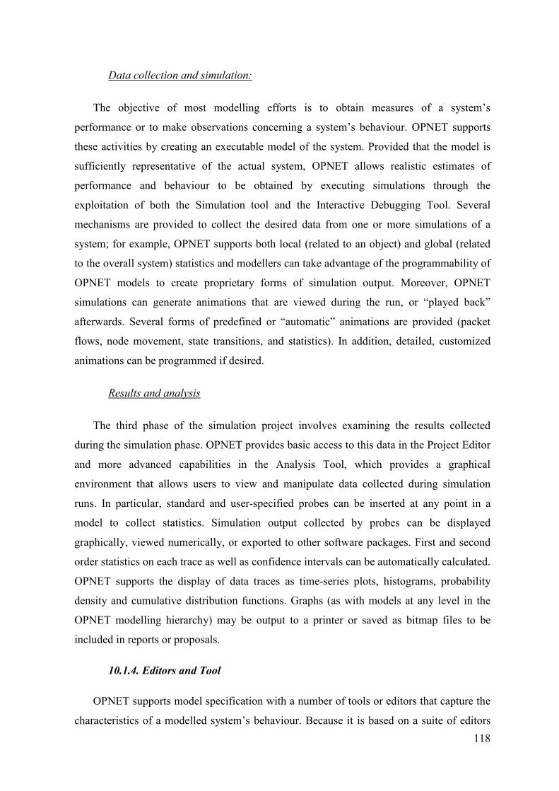
118

Data collection and simulation:

The objective of most modelling efforts is to obtain measures of a system’s

performance or to make observations concerning a system’s behaviour. OPNET supports

these activities by creating an executable model of the system. Provided that the model is

sufficiently representative of the actual system, OPNET allows realistic estimates of

performance and behaviour to be obtained by executing simulations through the

exploitation of both the Simulation tool and the Interactive Debugging Tool. Several

mechanisms are provided to collect the desired data from one or more simulations of a

system; for example, OPNET supports both local (related to an object) and global (related

to the overall system) statistics and modellers can take advantage of the programmability of

OPNET models to create proprietary forms of simulation output. Moreover, OPNET

simulations can generate animations that are viewed during the run, or “played back”

afterwards. Several forms of predefined or “automatic” animations are provided (packet

flows, node movement, state transitions, and statistics). In addition, detailed, customized

animations can be programmed if desired.

Results and analysis

The third phase of the simulation project involves examining the results collected

during the simulation phase. OPNET provides basic access to this data in the Project Editor

and more advanced capabilities in the Analysis Tool, which provides a graphical

environment that allows users to view and manipulate data collected during simulation

runs. In particular, standard and user-specified probes can be inserted at any point in a

model to collect statistics. Simulation output collected by probes can be displayed

graphically, viewed numerically, or exported to other software packages. First and second

order statistics on each trace as well as confidence intervals can be automatically calculated.

OPNET supports the display of data traces as time-series plots, histograms, probability

density and cumulative distribution functions. Graphs (as with models at any level in the

OPNET modelling hierarchy) may be output to a printer or saved as bitmap files to be

included in reports or proposals.

10.1.4. Editors and Tool

OPNET supports model specification with a number of tools or editors that capture the

characteristics of a modelled system’s behaviour. Because it is based on a suite of editors

119

that address different aspects of a model, OPNET is able to offer specific capabilities to

address the diverse issues encountered in networks and distributed systems. To present the

model developer with an intuitive interface, these editors break down the required

modelling information in a manner that parallels the structure of actual network systems.

Thus, the model-specification editors are organized in an essentially hierarchical fashion.

Model specifications performed in the Project Editor rely on elements specified in the Node

Editor; n turn, when working in the Node Editor, the developer makes use of models

defined in the Process Editor. The remaining editors are used to define various data models,

typically tables of values, that are later referenced by process or node level models. This

organization is depicted in the following list:

• Project Editor: the Project Editor is used to construct and edit the topology of a

communication network model. A network model contains only three fundamental

types of objects: sub-networks, nodes, and links. There are several varieties of nodes

and links, each offering different basic capabilities. In addition, each node or link is

further specialized by its “model”, which determines its behaviour and functionality.

The Project editor also provides basic simulation and analysis capabilities. Finally,

it’s worth highlighting that the entire system to be simulated is specified by the

corresponding network model;

• Node Editor: the Node Editor is used to specify the structure of device models.

These device models can be instantiated as node objects in the Network Domain

(such as computers, packet switches, and bridges). In addition to the structure, the

node model developer defines the interface of a node model, which determines what

aspects of the node model are visible to its user. This includes the attributes and

statistics of the node model. Nodes are composed of several different types of

objects called modules. At the node level, modules are “black boxes” with attributes

that can be configured to control their behaviour. Each one represents particular

functions of the node’s operation and they can be active concurrently. Several types

of connections (packet streams, statistical wires and logical associations) support

flow of data and control information between the modules within a node. The

following picture represents a generic Node Model:

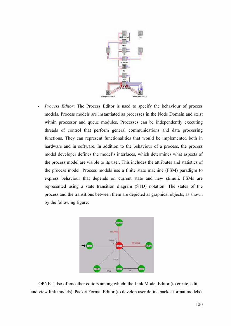
120

• Process Editor: The Process Editor is used to specify the behaviour of process

models. Process models are instantiated as processes in the Node Domain and exist

within processor and queue modules. Processes can be independently executing

threads of control that perform general communications and data processing

functions. They can represent functionalities that would be implemented both in

hardware and in software. In addition to the behaviour of a process, the process

model developer defines the model’s interfaces, which determines what aspects of

the process model are visible to its user. This includes the attributes and statistics of

the process model. Process models use a finite state machine (FSM) paradigm to

express behaviour that depends on current state and new stimuli. FSMs are

represented using a state transition diagram (STD) notation. The states of the

process and the transitions between them are depicted as graphical objects, as shown

by the following figure:

OPNET also offers other editors among which: the Link Model Editor (to create, edit

and view link models), Packet Format Editor (to develop user define packet format models)

121

and Antenna Pattern Editor(to create, edit, and view antenna patterns for transmitters and

receivers).

10.2. Model Specification

In this chapter the simulated Model, including the Network model, the QoS policy and

the implemented Supervisor and Requirement Agent algorithms are described.

10.2.1. Network model: the Dumbbell network

All the networks described in Chapter 9 (Cellular, Ad-hoc and Fixed Access Network),

even though different among them, have in common a same basic layout: a bottleneck link,

characterized by a limited capacity, on which many applications can transmit. For this

reason, without loss of generality, we decided to test our framework with the so called

“Dumbbell network”, shown in the following Figure:

Transmitter #1

Transmitter #2

Transmitter #3

Transmitter #N

.

.

.

.

.

.

Receiver #1

Receiver #2

Receiver #3

Receiver #N

Router West Router East

Bottleneck

Figure 14 - Dumbbell network

A generic dumbbell network is made of N transmitters (the workstations on the left of

the figure) connected to N receivers (the workstations on the right of the figure) by a

bottleneck (the central link between the two routers). The presence of a bottleneck link in

all the scenarios introduced so far allows us to use this simple model to study the

performance of the introduced Cognitive Application Interface in a generic access network.

122

Moreover, the Dumbbell Network is recognized in literature as a good benchmark for

testing new algorithms or new development in telecommunication (for example, see [Sh]

and [Da]). For the sake of clarity, we hereinafter report a table highlighting the

correspondences among the Dumbbell network elements shown in Fig. 9 (Workstations,

Routers and wired link) and the devices relevant to the networks described in Chapter 10.

Fixed Access

Network Cellular Network Ad-hoc Network

Transmitters Fixed Terminals Mobile Terminals Mobile Terminals

Router East Gateway Base Station Cluster Coordinator

Mobile

Router West-

Bottleneck Wired Link Wireless Link Wireless Link

It is worth stressing that, as highlighted in Chapter 9, when considering the “uplink-

side” (communications from Terminals to the Gateway or Base Station), the Requirement

Agents relevant to applications running in different Terminalshave to be placed in different

physical positions so they cannot exchange information one another, thus justifying the

adopted non cooperative Q-learning based solution.

10.2.2. QoS policy

OPNET controls the Quality of Service of a generic application by means of two

correlated processes: firstly, to each packet relevant to the application is associated a value

representing its Class of Service and secondly each router implements a scheduling policy

that allows to manage with different priorities packets belonging to different Classes of

Service.

The first task is accomplished by the IP layer of the workstation or server on which the

particular application runs: the IP layer inserts into a proper field of the IP header a value

representing the Class of Service of the packet. OPNET allows to define this value in two

ways: the user can set the Type of Service (ToS) of the application (Best Effort,

Background, Standard, Excellent Effort, Streaming Multimedia, Interactive Multimedia,

Interactive Voice, Reserved) or the Differentiated Service Code Point (DSCP). In this thesis

the latter method is used.

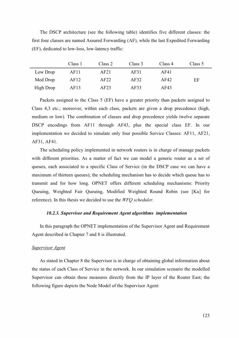
123

The DSCP architecture (see the following table) identifies five different classes: the

first four classes are named Assured Forwarding (AF), while the last Expedited Forwarding

(EF), dedicated to low-loss, low-latency traffic:

Class 1 Class 2 Class 3 Class 4 Class 5

Low Drop AF11 AF21 AF31 AF41

EF Med Drop AF12 AF22 AF32 AF42

High Drop AF13 AF23 AF33 AF43

Packets assigned to the Class 5 (EF) have a greater priority than packets assigned to

Class 4,3 etc.; moreover, within each class, packets are given a drop precedence (high,

medium or low). The combination of classes and drop precedence yields twelve separate

DSCP encodings from AF11 through AF43, plus the special class EF. In our

implementation we decided to simulate only four possible Service Classes: AF11, AF21,

AF31, AF41.

The scheduling policy implemented in network routers is in charge of manage packets

with different priorities. As a matter of fact we can model a generic router as a set of

queues, each associated to a specific Class of Service (in the DSCP case we can have a

maximum of thirteen queues); the scheduling mechanism has to decide which queue has to

transmit and for how long. OPNET offers different scheduling mechanisms: Priority

Queuing, Weighted Fair Queuing, Modified Weighted Round Robin (see [Ku] for

reference). In this thesis we decided to use the WFQ scheduler.

10.2.3. Supervisor and Requirement Agent algorithms implementation

In this paragraph the OPNET implementation of the Supervisor Agent and Requirement

Agent described in Chapter 7 and 8 is illustrated.

Supervisor Agent

As stated in Chapter 8 the Supervisor is in charge of obtaining global information about

the status of each Class of Service in the network. In our simulation scenario the modelled

Supervisor can obtain these measures directly from the IP layer of the Router East; the

following figure depicts the Node Model of the Supervisor Agent:

124

Figure 15 - Supervisor Agent: Node Model

The red links are called “statistic wire” and represent information exchanged by

processes in the same node (in other words they do not represent a communication

channel). Each of this link communicates to the Supervisor both the total traffic admitted

and the delay experienced in the associated queue for each Class of Service. These global

measures are then pre-processed by the Supervisor and sent to each Requirement Agent by

means of the Status Signal. The Internal Model (or Process Model) of the Supervisor is

depicted in the next picture:

Figure 16 - Supervisor Agent: Process Model

The pseudo-code representing the procedures encoded in the previous FMS is also

given (this code is relevant to the i-th queue associated with the i-th Service Class):

/*Counter for number of packets arrived at the queue

packet_counter=0;

/*Delay experienced by packet transmitted in the queue

delay_counter=0;

125

/*Size of packet transmitted

traffic_counter=0;

/*Each Tl seconds the supervisor updates the status signal

/* The computation of the Traffic Admitted and Delay is performed during an interval

/*ofduration Tmonit-l

for t→[T; T+Tl)

if (t< T+Tmonit-l&& +packet_transmission==true)

packet_counter++;

delay_counter=delay_counter+current_delay;

traffic_counter=traffic_counter+current_traffic;

endif

endfor

/*Update traffic admitted and average delay (we consider also the overhead introduced by

mac level)

traffic_admitted=(traffic_counter+ 208*packet_counter)/Tmonit-l;

delay=delay_counter/packet_counter;

/*Update status signal

put(traffic_admitted, i, status_signal);

put(delay, i, status_signal);

send_to_Agents(status_signal);

T= T+Tl;

For the queue i, the Supervisor Agent counts the number of packets transmitted

(variable packet_counter), the total delay experienced by each packet (delay_counter) and

the total traffic admitted, in bit (traffic_counter) during the period of duration Tmonit-l. Then,

by using these values, the Supervisor computes the traffic admitted and the delay

experienced by the i-th Service Class. It is worth stressing that, as highlighted in Chapter 8,

the values relative to Traffic Admitted and Delay are computed by the Supervisor Agent by

exploiting measurements taken in the time interval of duration Tmonit-l, where Tmonit-l can in

general be different from Tl. We made the reasonable hypothesis that the bigger part of the

126

delay experienced by packets is due to the time they wait in these queues or, in other words,

that the processing and transmission delay is not relevant.

It is worth reminding that, as described in Chapter 9, in real implementations, delay and

bit rate of the admitted traffic can be computed by monitoring the performance of the so-

called probe applications.

Requirement Agent

The modelled Requirement Agent is in charge of taking decisions about which Class of

Service is more suitable for the corresponding application. It includes (i) the sensingand

elaborationfunctionalities that allow to measure the QoEexperienced by the application,

and (ii) the control algorithm that, on the basis of the above-mentioned measure and of the

Status Signal received from the Supervisor Agent, has to select the appropriate Class of

Service.

The sensing functionalities have been implemented in OPNET as shown in the

following:

Figure 17 - Sensing Functionalities: Node and Process Editor

The sensing process obtains from the MAC layer the bits admitted in the network

and from the IP layer the delay experienced by packets. By using this information, the

modelled Requirement Agent can compute the QoE of the application that is used by the

control algorithm.

It is worth reminding, that in real implementations, the above-mentioned sensing

functionalities will be provided by the Sensing functionalities of the Cognitive Managers,

and the QoS parameters will be provided by the Elaboration functionalities of the Cognitive

Managers (see Chapter 3).

127

Figure 18 - Elaboration Functionalities: Node and Process Editor

Then, the selected control algorithm consists in a Q-learning algorithm (as illustrated in

paragraph 5.5.6). By using such algorithm the Requirement Agent selects the most

appropriate Class of Service; this control is then enforced to the IP layer changing the

DSCP field relative to the Class of Service in the IP header (the red statistic wire in the

former picture).

The procedures just introduced can be summarized in the subsequent pseudo-code:

/*The Agent computes QoE for each Service Class using the status signal

receive_from_Supervisor(status_signal);

for i→[1;number_CoS]

QoE_super(i)=update_QoE(status_signal, i);

endfor

packet_counter=0;

delay_counter=0;

traffic_counter=0;

/*The Agent computes the QoE of its application by exploiting measurements taken in an

interval of duration Tmonit-s

for t→[T; T+Ts)

if (t< T+Tmonit-s&& +packet_transmission==true)

packet_counter++;

delay_counter=delay_counter+current_delay;

traffic_counter=traffic_counter+current_traffic;

128

endif

endfor

traffic_admitted=(traffic_counter+208*packet_counter)/Tmonit-s;

delay=delay_counter/packet_counter;

QoE=update_QoE(traffic_admitted, delay);

/*The Agent computes the current state and reward from QoE and update the Q-value

matrix

agent_state=create_state(QoE, QoE_super);

reward=compute_reward(QoE, QoE_target);

reinforcement_learning(agent_state, agent_state_past, action_past);

/*The Agent takes an action on the basis of an є-greedy policy

action_past=compute_next_action(agent_state);

agent_state_past=agent_state;

T=T+Ts;

During the period of duration Tmonit-s the Requirement Agent counts the number of

packets transmitted (variable packet_counter), the total delay experienced by each packet

(delay_counter) and the total traffic admitted, in bit (traffic_counter). Then, by using these

values, the Requirement Agent computes the admitted traffic and the delay experienced by

its associated application. It is worth stressing that, as highlighted in Chapter 8, the

measures relative to Admitted Traffic and Delay are computed by the Requirement Agent

by exploiting measurements taken in the time interval of duration Tmonit-s.

The method update_QoE uses the weighted QoE function defined in chapter 8.2 to

update the QoE both for the applications controlled by the Requirement Agent, named QoE,

and both for the i-th Service Class (by means of the Status Signal transmitted by the

Supervisor Agent), namedQoE_super, using the measured Traffic Admitted and Delay. In

this thesis we do not consider the Loss Rate for the reasons illustrated in the following

Chapter.

The method compute_reward has the task of computing the reward, through the

measured Quality of Experience QoE and the target one,QoE_target,using thefirst reward

functiondefined in chapter 7.3.

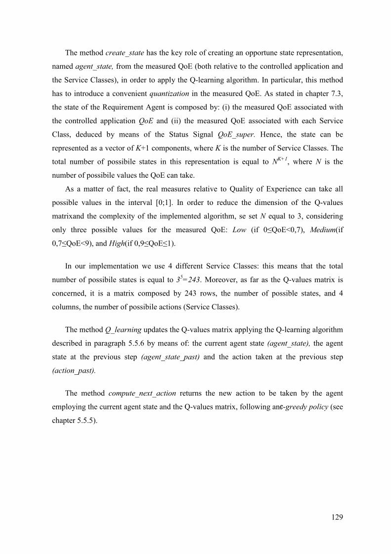
129

The method create_state has the key role of creating an opportune state representation,

named agent_state, from the measured QoE (both relative to the controlled application and

the Service Classes), in order to apply the Q-learning algorithm. In particular, this method

has to introduce a convenient quantization in the measured QoE. As stated in chapter 7.3,

the state of the Requirement Agent is composed by: (i) the measured QoE associated with

the controlled application QoE and (ii) the measured QoE associated with each Service

Class, deduced by means of the Status Signal QoE_super. Hence, the state can be

represented as a vector of K+1 components, where K is the number of Service Classes. The

total number of possibile states in this representation is equal to NK+1

, where N is the

number of possibile values the QoE can take.

As a matter of fact, the real measures relative to Quality of Experience can take all

possible values in the interval [0;1]. In order to reduce the dimension of the Q-values

matrixand the complexity of the implemented algorithm, se set N equal to 3, considering

only three possible values for the measured QoE: Low (if 0≤QoE<0,7), Medium(if

0,7≤QoE<9), and High(if 0,9≤QoE≤1).

In our implementation we use 4 different Service Classes: this means that the total

number of possibile states is equal to 35=243. Moreover, as far as the Q-values matrix is

concerned, it is a matrix composed by 243 rows, the number of possible states, and 4

columns, the number of possibile actions (Service Classes).

The method Q_learning updates the Q-values matrix applying the Q-learning algorithm

described in paragraph 5.5.6 by means of: the current agent state (agent_state), the agent

state at the previous step (agent_state_past) and the action taken at the previous step

(action_past).

The method compute_next_action returns the new action to be taken by the agent

employing the current agent state and the Q-values matrix, following anє-greedy policy (see

chapter 5.5.5).

130

11. SIMULATION RESULTS

This chapter describes the simulated scenarios and illustrates the results obtained

implementing the innovative QoE control framework introduced in this thesis.

11.1. Reference Scenario and key parameters

This chapter shows the performance of the approach described in this thesis

highlighting the enhancements of a dynamic association between Applications and Service

Classes(hereinafter this case will be referred to as dynamic case) with respect to the static

case.

In the dynamic case each Application can dynamically change its Service Class, by

means of the reasoning embedded in the Cognitive Application Interface as described in

Chapters7 and 8, whilst in the static case the application interface just provides a static

mapping between Applications and the most suitable Service Classes.

The simulated framework is the Dumbbell networkdescribed in Chapter 10.

We have considered two Application types: “Video Conference” and FTP, two built-in

Opnet types.

In this respect, we have simulated the following scenarios:

• Single-Application Scenario: three “Video Conference” Applications transmit on a

channel with capacity C equal to 7 Mbit/sec, for 700 seconds. We simulate both the

static and the dynamic cases with different levels of network traffic;

• Multi-Application Scenario: two “Video Conference” applications and one FTP

application transmit on a channel with capacity C equal to 7 Mbit/sec, for 700

seconds. We simulate both the static and the dynamic cases, with different levels of

network traffic.

The following table, referring to the parameters introduced in Chapters 5,7 and 8,

summarizes the selected values for Opnet implementation:

131

Q-learning algorithm QoE Computation

(weights) Tl-

Tmonit-l

(sec)

Ts-

Tmonit-s

(sec) Learning

Rate

Discount

Factor

Exploring

Factor αααα1 αααα2 αααα3

Requirement

Agent 1/k 0.7 0.1 0.5 0.5 0 - 2

Supervisor

Agent - - - - - - 40 -

The previous table shows that the coefficientα3, related to the Loss Rate parameter in

the QoE computation (see chapter 8.2), has been set to zero: this means that our simulations

do not consider the Loss Rate in QoE computation. This choice can be justified by several

evidences: (i) in wired networks the BER(Bit Error Rate) is negligible, while in wireless

networks the most advanced physical link techniques (encoding, modulation, shadowing

control, etc.) techniques allow a strict BER control (i.e. the measured BER is, in almost

situations, lower than the maximum tolerated one), (ii) for Loss rate critical Applications

the possible presence of the transport layer protocol TCP, in charge of retransmitting loss or

damaged packets, further contributes to keep Loss Rate strictly controlled, (iii) traffic

overflow at queue level is limited by proper dimensioning of queue lengths.

As shown in the previous table, both for the Supervisor and Requirement Agent,Tmonit-l

and Tmonit-s have been chosen equal respectively to the periods Tl and Ts(see Chapter 8).

This means that the monitoring period, during which the measurements to compute QoE are

collected, and the control period, at the end of which the Service Class is selected, are

equal.

As far as the Learning Rate is concerned, we chose a sequence that satisfies the

stochastic approximation conditions described in paragraph 5.5.4. At this proposal, we have

to point out that, in our scenario, it is recommended to restart the learning process if the

performance obtained by the Requirement Agent is poor, since we are dealing with an

Environment that can vary due to the presence of other Agents. For the same reason, in real

implementations, the Agents have never to completely stop the learning process.

132

11.2. Single-Application Scenario

As previously introduced, this scenario considers three “Video Conference”

Applications transmitting on a channel with capacity C equal to7 Mbit/sec.

Considering that, as stated in the previous chapter, we assume α3=0, the measures used

to compute QoE are the admitted traffic Radm and the experienced delay D, or better the

difference among these values and the corresponding thresholds, namely Radm-min (minimum

guaranteed bit rate), and Dmax (maximum transfer delay). We have assumed that these

thresholds are equal for the three Video Applications: the only difference among them lies

in the fact that we have assigned three different levels of QoEtarget; note that, in the static

case these three different levels correspond to the static mapping of the three Applications

in three different Service Classes. In general, in the static case, no Service Class is able to

guarantee the specific QoE target required by the relevant application: the only issue a

Service Class is able to guarantee is a different priority among applications; for this reason

the application associated with the highest QoE target will be assigned to the highest

available Service Class and so on.

It is important to remark that in this thesis we do not implement the Application

Handler described in Chapter x. For this reason, as far as the QoE targets are concerned, we

assume the role of the Application Handler, setting up three different QoE targets (one for

each application), in order to represent three possible users with different requirements.

In order to analyse the behaviour of our algorithm, we simulate five different Traffic

Scenarios, ranging from a situation in which the bottleneck link is idle (Traffic Scenario

#1), to a situation in which the bottleneck link is very congested:

• Traffic Scenario #1: the sum of the applications minimum guaranteed bit rate

doesn’t exceed the link capacity (3Radm-min ≈ 0.85C);

• Traffic Scenario #2: the sum of the applications minimum guaranteed bit rate is

slightly higher than the link capacity (3Radm-min ≈ C);

• Traffic Scenario #3: the sum of the applications minimum guaranteed bit rate

exceeds the link capacity (3Radm-min ≈ 1.3C);

133

• Traffic Scenario #4 and #5: the sum of the applications minimum guaranteed bit rate

greatly exceed the link capacity (3Radm-min ≈ 1.5C in Scenario #4 and 3Radm-min ≈ 1.8C

in Scenario #5).

11.2.1. Traffic Scenario #1

The following table illustrates the main parameters of the three Video Applications

used to simulate traffic inScenario #1:

Roffered

(bits/sec)

Radm-min

(bits/sec) Dmax (sec) QoEtarget

Service

Class

Video #1 4300000 2000000 0.18 0.99 AF41

Video #2 4300000 2000000 0.18 0.94 AF31

Video #3 4300000 2000000 0.18 0.89 AF21

Figures19 and 20 refer to the static and dynamic cases, respectively. The simulations

report the Measured QoE value as a function of the simulation time, and refer to the so-

called Averaged QoE, which is deduced by averaging the QoE measured in the time

interval ranging from the beginning of simulation till the current simulation time.

The graphs are relevant since we are primarily interested in achieving an average QoE

that converges to the targetQoE. As a matter of fact, the network operators policy has not

the aim of providing to users a QoE value that is equal to the QoE target at each time

instant; instead, the network operators policy’s aim is that of guaranteeing to users an

average QoE as far as possible close to the QoE target. The average is computed over a

time slot that can change according to the user and/or the application type.

As stated at the beginning of the paragraph, in Traffic Scenario #1 the sum of the

minimum guaranteed bit rates for the applications does not exceed the link capacity. For

this reason, in the static scenario (Figure 19), the applications Video #1, Video #2 and

Video #3 reach a value of QoE equal to one. This is due to the fact that, since the channel is

not congested, the QoS policy implemented in Router East is always able to admit at least

the minimum guaranteed bit rate for each application. Moreover, also the delay experienced

by Video applications is always lower than the maximum admitted delay. Also in this

circumstance, this is due to the fact that the channel is not congested and the waiting time

134

inside the queues is negligible. This entails that, in the QoE computation with the formula

7.1, the value obtained in the static case is equal to one. In the dynamic case the aim of the

algorithm is to reduce, as much as possible, the error between the obtained QoE and the

target QoE. As Figure 20 depicts, Video #1 (the higher priority application) reaches the

same average QoE of the static case. As far as Video #2 and Video #3 are concerned, the

QoE values obtained are lower than the static case but closer to QoE target.

The following table reports the percentage errors (differences between the average QoE

and the target QoE at the end of simulation, normalized with respect to the QoE target)

obtained at the end of the simulation:

Video #1 Video #2 Video #3

Static Case 1% 6% 12%

Dynamic Case 1% 3% 7%

Table 1: Scenario 1 - Percentage Error

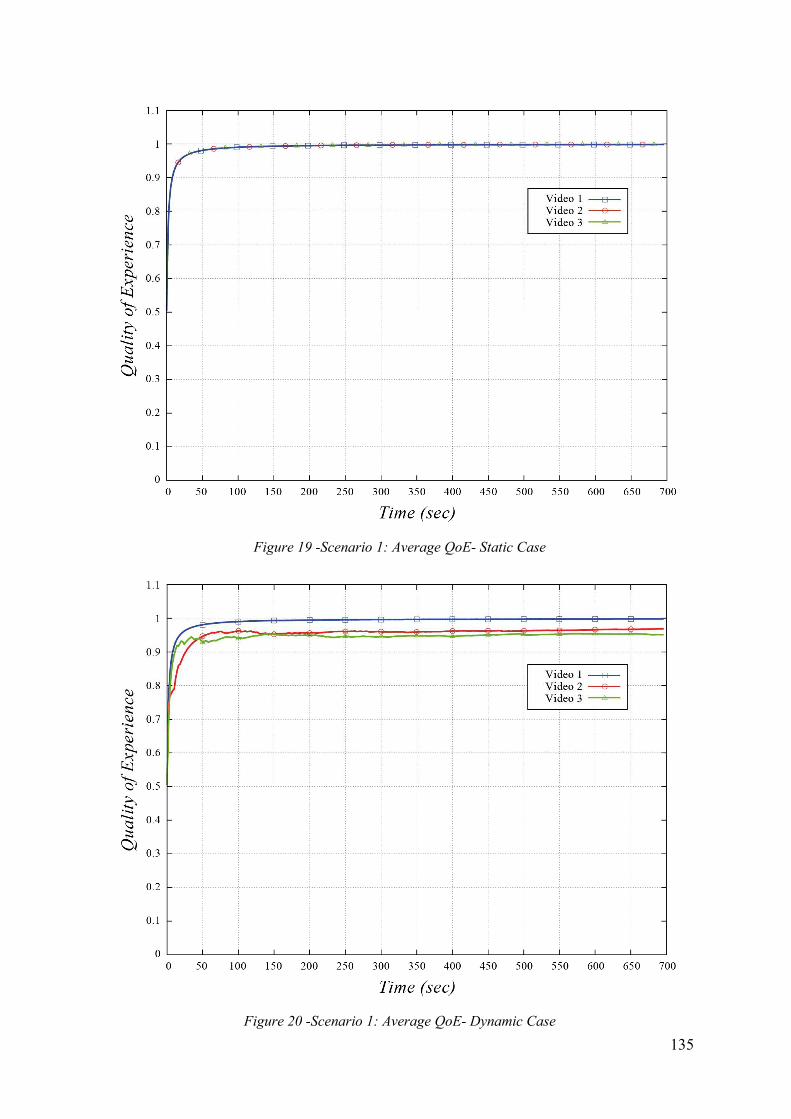
135

Figure 19 -Scenario 1: Average QoE- Static Case

Figure 20 -Scenario 1: Average QoE- Dynamic Case

136


The following table illustrates the main characteristics of the three Video applications

used to simulate traffic in Scenario #2:

Roffered

(bits/sec)

Radm-min


Service

Class

Video #1 4300000 2500000 0.18 0.99 AF41

Video #2 4300000 2500000 0.18 0.94 AF31

Video #3 4300000 2500000 0.18 0.89 AF21

In this case we simulate the network at the limit of congestion, since the sum of the

minimum guaranteed bit rate barely exceeds the link capacity.

In this Scenario it is evident that a dynamic choice of Service Classes entails better

performance with respect to a static association. In the Static case (Figure 21) the different

priority (due to different Service Classes) given to the Video applications is evident: Video

#1 obtains the higher QoE, then respectively Video #2 and Video #3. Even in a low

congestion scenario, a static approach is not able to guarantee a value of QoE close to the

target, especially for Video #2 and #3 (see Table 2). The performance worsening with

respect to Scenario #1 is mainly due to the network congestion. In Scenario #2, the sum of

the minimum guaranteed bit rates exceeds the link capacity; this obviously entails that it is

impossible to admit for all applications the required bit rate. Similarly, also the queuing

time increases (the channel works as a bottleneck causing packets wait in the relevant queue

until transmission) and this leads to a poor QoE, especially for low priority applications.

Analogous considerations are valid also in the dynamic case (Figure 22). Despite that,

even though the QoE does not converge to the target, the QoE values obtained in the

dynamic case are higher than the values reached in the static one. This is due to the

opportunity for applications to dynamically change their Service Class according to the

congestion level of the network. Both from Figure 22 and Table 2 can be noted that the

algorithm is very effective especially for Video #2 and Video #3, while Video #1 obtains

similar outcome both in static and dynamic case. This result is caused by the fact that in the

static case Video #1 is associated to the highest priority class and consequently it obtains

137

the highest bit rate and the lowest delay achievable in the network. For this reason, the QoE

attained in the static case by Video #1 represents a sort of “upper limit”, that is very

challenging to overcome. Nevertheless, also in the dynamic case, the same value of QoE

with respect to the static case is reached (the % error is the same), thus highlighting the

effectiveness of our approach. The following table reports the percentage errors obtained at

the end of the simulation:


Static Case -4% -12% -20%

Dynamic Case -4% -5% -3%

Table 2 - Scenario 2: Percentage Error

138

Figure 21–Scenario 2: Average QoE- Static Case

Figure 22–Scenario 2: Average QoE- Dynamic Case

139



used to simulate traffic in Scenario #3:

Roffered

(bits/sec)

Radm-min


Service

Class

Video #1 4300000 3000000 0.18 0.99 AF41

Video #2 4300000 3000000 0.18 0.94 AF31

Video #3 4300000 3000000 0.18 0.89 AF21

As expected, as the traffic increases, the performance deteriorates, especially in the

static case (similar considerations with respect to Scenario #2 can be repeated). Even in this

scenario, a dynamic approach performs better than a static association, and an improvement

can be noted also for Video #1 (see Figure 24 and Table 3). Another aspect to highlight is

the convergence time toward stable QoE values, that is always in an interval of sixty

seconds. This value seems acceptable also from a real implementation point of view. The

following table reports the percentage errors obtained at the end of the simulation:


Static Case -12% -20% -27%


Table 3 -Scenario 3: Percentage Error

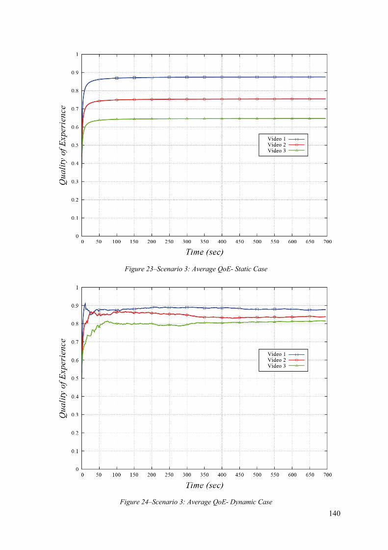
140

Figure 23–Scenario 3: Average QoE- Static Case


141

11.2.4. Traffic Scenario #4 and #5


used to simulate traffic in Scenario #4 and #5:

Roffered

(bits/sec)

Radm-min (bits/sec) Dmax

(sec) QoEtarget

Service

Class Scenario

#4

Scenario

#5

Video #1 4300000 3500000 4200000 0.18 0.99 AF41

Video #2 4300000 3500000 4200000 0.18 0.94 AF31

Video #3 4300000 3500000 4200000 0.18 0.89 AF21

These are very demanding scenarios since the sum of the applications minimum

guaranteed bit rates greatly exceed the link capacity. As Figure 25 and 27 show, even the

highest priority application Video #1 achieves a low QoE in the static case. Better results

are accomplished in the dynamic case (figures 26 and 28), especially for Video #2 and #3;

an improvement is evident also for Video #1, in both scenarios, thus underlining that the

performance of the dynamic approach versus the static one improves as more as the

network is congested. Tables 4 and 5 report the percentage errors for Scenario #4 and #5.

Graphs 26 and 28(dynamic case) show an initial phase where Video #2 and Video #3

achieve similar values of QoE or Video #3 performs better than Video #2, even though the

latter has a higher QoE target. This behaviour can be caused by: (i) the high level of

congestion: the applications are trying to admit an amount of traffic that greatly exceed the

capacity C and this makes the task of the Requirement Agents very difficult, (ii) the

learning process embedded in the Requirement Agents, that, starting without an a priori

knowledge on Environment dynamics and state-action value matrix, entails an initial phase

of exploration and learning, and (iii) a lack of coordination among agents since, as already

mentioned, Q-learning is not a multi-agent algorithm. This entails that it is possible for low

priority applications to perform better than high priority applications.

Despite that, after the transitory phase, the agents are autonomously able to restore the

correct hierarchy.

142

The following tables report the percentage errors obtained at the end of the simulations:

Scenario #4


Static Case -18% -25% -32%


Scenario #5


Static Case -25% -30% -38%


Tables4 and 5 -Scenarios 4 and 5: Percentage Error

143

Figure 25–Scenario 4:Average QoE- Static Case


144

Figure 27–Scenario 5:Average QoE- Static Case


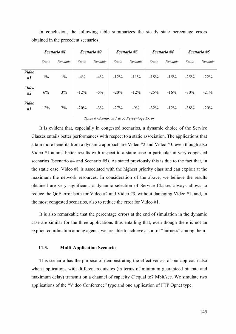
145

In conclusion, the following table summarizes the steady state percentage errors

obtained in the precedent scenarios:

Scenario #1 Scenario #2 Scenario #3 Scenario #4 Scenario #5

Static Dynamic Static Dynamic Static Dynamic Static Dynamic Static Dynamic

Video

#1 1% 1% -4% -4% -12% -11% -18% -15% -25% -22%

Video

#2 6% 3% -12% -5% -20% -12% -25% -16% -30% -21%

Video

#3 12% 7% -20% -3% -27% -9% -32% -12% -38% -20%

Table 6 -Scenarios 1 to 5: Percentage Error

It is evident that, especially in congested scenarios, a dynamic choice of the Service

Classes entails better performances with respect to a static association. The applications that

attain more benefits from a dynamic approach are Video #2 and Video #3, even though also

Video #1 attains better results with respect to a static case in particular in very congested

scenarios (Scenario #4 and Scenario #5). As stated previously this is due to the fact that, in

the static case, Video #1 is associated with the highest priority class and can exploit at the

maximum the network resources. In consideration of the above, we believe the results

obtained are very significant: a dynamic selection of Service Classes always allows to

reduce the QoE error both for Video #2 and Video #3, without damaging Video #1, and, in

the most congested scenarios, also to reduce the error for Video #1.

It is also remarkable that the percentage errors at the end of simulation in the dynamic

case are similar for the three applications thus entailing that, even though there is not an

explicit coordination among agents, we are able to achieve a sort of “fairness” among them.

11.3. Multi-Application Scenario

This scenario has the purpose of demonstrating the effectiveness of our approach also

when applications with different requisites (in terms of minimum guaranteed bit rate and

maximum delay) transmit on a channel of capacity C equal to7 Mbit/sec. We simulate two

applications of the “Video Conference” type and one application of FTP Opnet type.

146

In order to analyse the behaviour of our algorithm, we simulate two different Traffic

Scenarios, similar to Scenario #2 and #3 of the previous section as far as the total minimum

admitted bit rate is concerned:

• Traffic Scenario#1: the sum of the applications minimum guaranteed bit rate is

slightly higher than the link capacity (∑Radm-min ≈ C);

• Traffic Scenario#2: the sum of the applications minimum guaranteed bit rate

exceeds the link capacity (∑Radm-min ≈ 1.4C);


The following table illustrates the main characteristics of the three applications used to

simulate traffic in Scenario #1:

Roffered

(bits/sec)

Radm-min


Service

Class

Video #1 2850000 2200000 0.15 0.99 AF41

Video #2 2850000 2200000 0.15 0.89 AF21

FTP 4200000 3700000 0.5 0.97 AF31

The main difference with respect to the Single-Application scenarios is the presence of

two type of applications with different requisites: Video Applications require a low delay

and a minimum guaranteed bit rate that is smaller than the minimum guaranteed bit rate of

FTP application. On the contrary, the FTP Application has not a demanding constraint on

the delay, but requires a high guaranteed bit rate.

In this scenario the network is congested and this explains why, also in the static case,

the QoE obtained is very low, especially for Video #2 (equivalent considerations with

respect to the Single-Application Scenario are valid also for this case). Both Figure 30 and

Table 7 show that a dynamic association between applications and Service Classes entails

better performance with respect to a static association. The QoE error is reduced for every

application, especially for Video #2 and FTP.

It can be observed from Figure 30 that, in the dynamic case, there is a transitory phase

during which Video #2 performs better than FTP. This behaviour can be due to causes

147

similar to those illustrated in paragraph 11.2.4 for the Single-Application case, in particular

a lack of coordination among agents. In the following Chapter a different Reinforcement

Learning Algorithm (Friend or Foe algorithm) will be introduced aiming at reducing this

problem. Despite that, also a simple Q-learning algorithm, after an initial learning phase, is

able to recover the correct priority among applications.

Video #1 Video #2 FTP

Static Case -10% -22% -16%


Table 7: Scenario 1: Percentage Error

148

Figure 29 - Scenario 1: Average QoE - Static Case

Figure 30 - Scenario 1: Average QoE - Dynamic Case

149


The following table illustrates the main characteristics of the three applications used to

simulate traffic in Scenario #2:

Roffered

(bits/sec)

Radm-min


Service

Class

Video #1 2850000 2700000 0.15 0.99 AF41

Video #2 2850000 2700000 0.15 0.89 AF21

FTP 4200000 4200000 0.5 0.97 AF31

As expected, the performance worsens, bothin the static and dynamic case, due to the

high level of congestion. Nonetheless, in confirmation of the results presented in the

previous paragraphs, the dynamic case performs better than the static one, both in terms of

percentage error reduction and in terms of “fairness” among applications (the percentage

errors for the three applications are similar).

It is also evident from Figure 32 that the applications reach a stable value of QoE nearly

after sixty seconds, a value that seems acceptable also as far as an implementation on real

devices is concerned.

Table 8 shows the QoE percentage errors obtained both in static and dynamic case:


Static Case -14% -32% -20%


Table 8 -Scenario 2: Percentage Error

150

Figure 31 - Scenario 2: Average QoE - Static Case

Figure 32 - Scenario 2: Average QoE - Dynamic Case

151

11.4. Conclusions

The results presented in this chapter clearly show that a dynamic control of Service

Classes allows to reduce, especially in congested scenarios, the error (difference between

the average QoE and the target QoE)and to guarantee higher “fairness” among applications

with respect to a static association between applications and Service Classes.

This is mainly due to the capability of the Requirement Agents (provided with a Q-

learning algorithm ) to learn and adapt their behaviour according to: (i) the local status of

the controlled application and (ii) the global status of the network, encoded into the Status

Signal and transmitted by the Supervisor Agent.

Moreover, it is worth stressing that the results illustrated in this thesis have been

obtained implementing a standard Q-learning algorithm, without any explicit coordination

signalling among agents with the exception of the Status Signal. This issue is important

especially as far as an implementation on real devices is concerned: (i) the only overhead is

introduced by the Status Signal and (ii) the Q-learning algorithm is very simple, scalable,

distributed and easily implementable in real devices.

152

12. AN ALTERNATIVE RL APPROACH: PROPOSED SOLUTION AND

PRELIMINARY RESULTS

In chapter 6.3 a proposal for overcoming some limitations of the Q-Learning

approachhas been introduced,based on the Friend-or-Foe Q-learning algorithm. In this

chapter a preliminary proposal of implementation of a Friend or Foe based solution is

presented and preliminary simulation results are illustrated.

12.1. Friend-or-Foe algorithm

The Friend-or-Foe Q-learning (FFQ) is a particular Reinforcement Learning algorithm

able to deal with Multiagent environments. This section illustrates the two-players version

of FFQ from the perspective of Agent 1.

As in a common Q-learning algorithm each agent has to choose an action, observe the

reward and update a table of Q-values. In FFQ-learning this update is performedaccording

to the following expression:

if the opponent is considered a friend and:

if the opponent is considered a foe.

As stated in chapter 6.3, in FFQ-learning it is assumed that the opponents are friends

(they work together to maximize agent’s value) or foes (they work together to minimize

agent’s value). To be able to update its Q-table each Agent has to know the state s, the

reward r, its action a1 but also the action a2 chosen by the other agent. This obviously

entails a sort of observation of the Agent 1 with respect to the Agent 2, and vice versa, or a

communication between the Agents. In our setting this is not feasible, since communication

among Agents is totally excluded: the only allowed signalling can be from the Supervisor

Agent to the Requirement Agents. For this reason, in the following paragraph we illustrate a

153

possible modification of the Supervisor Agent and Requirement Agent to deal with this

aspect.

It is worth stressing that a complete explanation of the FFQ-learning is beyond the aim

of this thesis and can be found in [Vi] and [Li-2].

12.2. Cognitive Application Interface implementation

In our setting each application is associated with a Requirement Agent, in charge of

dynamically selecting the most appropriate Service Class to guarantee the specific QoE

target. An explicit signalling among Agents is not allowed, consequently an Agent cannot

detect the actions selected by the other Agents and a standard implementation of FFQ-

learning is not possible. For this reason, in an implementation with FFQ algorithm, the

Supervisor Agent has the key roleof modelling a “Macro-Agent” representing the entire

cloud of Requirement Agents (and associated applications), as depicted in the following

figure (the figure refers to a Cellular Network, but similar considerations can be repeated

also for Fixed Access and Ad-hoc Networks):

Mobile Terminal 1

Mobile Terminal 2

Mobile Terminal 3

Base

Station

S

A

RA

1

AH

1

RA

2

AH

2

RA

3

AH

3

Mobile Terminal 4

RA

4

AH

4

Mobile Terminal 5

RA

5

AH

5

Macro-AgentAgent 1

Figure 33- Friend or Foe approach: The Macro-Agent

The Supervisor Agent has the key role of analysing the behaviour of the Requirement

Agents cloud and modelling the Macro-Agent. In this way, each Requirement Agent can

154

implement a FFQ algorithm in the two players case, where the two players are itself and the

Macro-Agent. We also suppose that that the traffic admitted by a single application is a

small fraction of the total traffic in the network, i.e. that a single application does not have

significant effects on the Macro-Agent. This supposition seems trustworthy in real

networks, where many devices transmit at the same time.

In order to implement the FFQ algorithm, we propose to consider the Macro-Agent as a

“foe”. This assumption is realistic since the applications, and the related Requirement

Agents, transmit on the same limited channel. This entails the consumption of a limited

common resource by the i-th application to the detriment of the other applications (and vice

versa) or, in other words, that the i-th application operate damaging the other applications

(and vice versa). Since the Macro-Agent is the representation of the other Requirement

Agents, the hypothesis that it is an opponent seems reasonable.

Another important aspect to highlight is that the signalling among the Supervisor and

the Requirement Agents has to occur at every time step ts the Requirement Agents take an

action. This is a necessary conditions in the FFQ-learning in order to update the Q-value

table, because also the action chosen by the other Agent has to be known (see chapter 6.3)

when the update is performed. This entails that the action selected by the Macro-Agent has

to be communicated to the Requirement Agents each time they chose an action and update

the Q-table, i.e. every ts seconds. For this reason, differently from the Q-learning

implementation, in this case the parameters Tl, Tmonit-l and Tmonit-s have to be chosen equal to

Ts, in order to evaluate the two actions’ effect in the period of duration Ts.

Supervisor Agent

In order to make possible the implementation of the FFQ algorithm in the Requirement

Agents, the Supervisor Agent has the key role of modelling the Macro-Agent and

communicating the action chosen by the Macro-Agent to the Requirement Agents. As

stated previously, the Macro-Agent is a global representation of the applications supported

by the network and it is not a real operating agent. The actions it can take are similar to

those of the Requirement Agents, i.e. to move the traffic from one Service Class to another;

but differently from the Requirement Agents, that have to move the entire traffic from one

Service Class to another, the Macro-Agent can choose to assign a fraction of the entire

traffic to different Service Classes. In other words, each ts seconds, the Macro-Agent can

assign a percentage equal to α(ts,1) of the whole traffic to the Class 1, equal to α(ts,2) of the

155

whole traffic to the Class 2 and so on; with the constrain that α(ts,1)+α(ts,2)+…+α(ts,K)=1

(where K is the total number of Service Classes).

In order to pursue this task, at each time ts,we propose that the Supervisor Agent

computes, for each Service Class k (from 1 to K),the admitted traffic Radm(ts,k). The

parameter Radm(ts,k) is computed by the Supervisor Agent by exploiting measurements

taken in the time interval [t-ts; t], where t is the current time. At each time ts the Supervisor

Agent broadcasts to the Requirement Agents a proper message, hereinafter referred to as

Action Signal and indicated as as(ts), i.e. a string of LK bits as the following:

as(ts) = [ α(ts,1), α(ts,2),…, α(ts,K)]

where L is the number of bits necessary to code α(ts,k) and K is the total number of

Service Classes. The parameter α(ts,k) is defined as the percentage of traffic admitted by the

Class of Service k and is computed as:

The signalling overhead introduced by the Action Signal consists in broadcasting LK

bits every Ts seconds, where Ts is the duration of the period between the broadcast of a

given status signal and the next one, i.e. Ts=ts+1-ts.

The Action Signal represents for the Requirement Agents the action chosen by the

Macro-Agent and is interpreted as the percentage of traffic the Macro-Agent has moved

into the different Service Classes.

Requirement Agent

The Requirement Agent, at each time ts, based on the action signal received by the

Supervisor Agent, has to select a Service Class.In order to perform the Service Class

selection, each Requirement Agent is provided with a Friend-or-Foe Q-learning algorithm.

In particular we refer to the foe version of the algorithm.Respect to the Q-Learning based

solution (see chapter 7.3), the Reinforcement Learning model will be modified as follows:

State and action spaces

For the state variables s, a suitable selection, at time ts,is the measured QoE

QoEmeas(ts,a), as defined in chapter 8.2 (“QoS case”).

156

Concerning the action space, the action a1 is the action selected by the Requirement

Agent (the proper Service Class), and the action a2 is the action selected by the Macro-

Agent, i.e. the Action Signal as(ts).

Reward function

The proposed reward function r(ts) is the first function asdescribed in chapter 7.3, that

is:

r(ts) = - [QoEmeas(ts,a)−QoEtarget(a)]2

12.3. Preliminary simulation results

The Figure 34 illustrates a preliminary simulation result obtained implementing the

proposed solution using a FFQ-learning algorithm.

The simulation refers to the Multi-Application Scenario#1 described in paragraph

11.3.1, highlighting the presence of a transitory phase during which Video #2 performs

better than FTP. In this case, the use of a FFQ-learning avoids this behaviour. The results

obtained in terms of QoE are similar to those obtained with a Q-learning implementation,

even though an improvement both for Video #1 and #2 can be noticed (see Table 9).


Static Case -10% -22% -16%

Dynamic Case

(Q-learning) -7% -4% -9%

Dynamic Case

(FFQ-learning) -5% -3 -9

Table 9 – Scenario 1 – Q-Learning versus FFQ: Percentage Error

Future experimentations are recommended in order to further investigate the

advantages of the alternative approach presented in this Chapter.

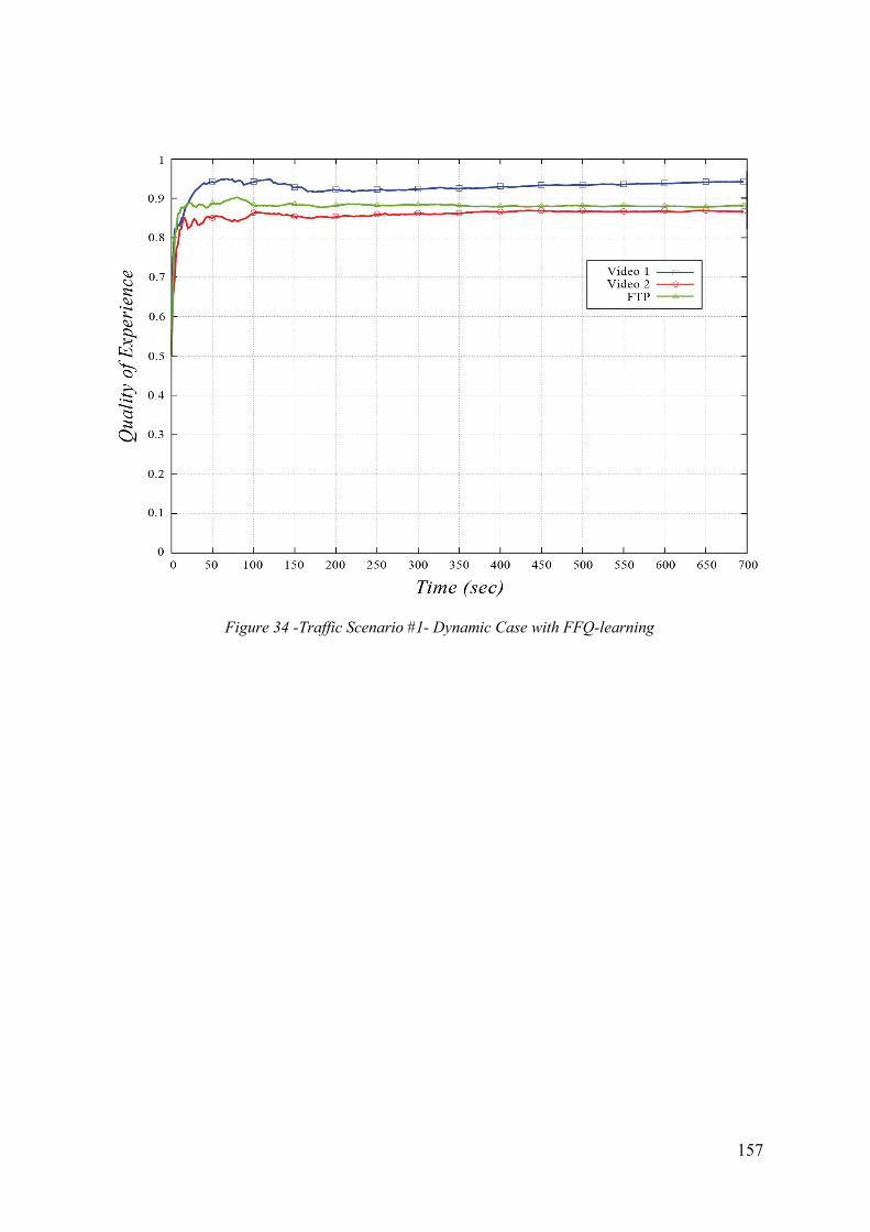
157

Figure 34 -Traffic Scenario #1- Dynamic Case with FFQ-learning

158

13. CONCLUSIONS

This workis aimed at defining an innovativeApplication Interface able to manage

“cognitive” Application Requirements, to be defined in terms of Quality of Experience

(QoE) Requirements.

The proposed Interface is based on three basic elements: the Application Handler, the

Requirement Agent and the Supervisor Agent.

The main element, from the “cognitive” point of view, is the so called Requirement

Agent. The Requirement Agent is in charge of dynamically selecting the most appropriate

Class of Service to be associated to the relevant application in order to “drive” the

underlying networks elements to satisfy the application QoE Requirements, that is reaching

(or approaching) the target QoE level. The QoE function is defined considering all the

relevant factors influencing the quality of experience level as it is perceived by the final

users for each specific Application (including Quality of Service, Security, Mobility and

other factors).

The Requirement Agent must be able to “learn”,based oninteraction with the

environment, to take optimal decisions regarding the Class of Service, in other words, the

agent must to solve a “Reinforcement Learning problem”:the key idea followed in the thesis

is modelling the Requirement Agent as a “Reinforcement Learning Agent”.

After a documentation regarding, on the one hand,different control, optimization, multi-

agent systems and machine learning theories and, on the other hand,availableSW platforms

and tools, the Author decided to adopt a model-free Reinforcement Learning approach,

based on the Q-Learning algorithm.

The Q-learning algorithm seems to be a really “cognitive” and “adaptive” solution to

the QoE problem, especially in the considered scenario, where the following key

assumptions and constraints must be considered: no a priori knowledge aboutthe

network/system model and dynamics, no coordination/communication among agents,

limited agent signalling, power, memory and computation capabilities.

Once defined the action space(in terms of Service Classes),in order to define the RL

model several state variables and reward functions were considered andanalysed.

159

The selected state variables (the measured QoE of the relevant Application and the

measured QoE of each Class of Service) allow to describe the current network situation to

the RL agent, while the proposed reward function is able to guarantee that the Class of

Service will be selected aiming at reaching the target QoE, meaning thatthe action (Class of

Service selection) will be changed (improved)aiming at reducing the difference between the

measured and target QoE (the quadratic error is considered).

For implementation and simulation purposes, the QoS case was considered: this is a

special case, where the Application QoE is defined in term of Quality of Service metrics. In

the QoS case, throughput, delay and loss rateparameters were considered: the proposed

QoE function assigns different weights to the QoS parameters and allows to guarantee a

satisfactory granularity in defining Application QoE requirements.

The proposed RL based solution was implemented and tested using OPNET, a license-

based network and traffic simulation platform widely used in the ICT field; the proposed

Supervisor and Requirement algorithms were implementedon OPNET using the supported

version of C++

language.Several simulationswere run in order to test functionality and

performance of the proposed Cognitive Application Interface and algorithms, considering

single and multiple applicationscenarios with different network congestion levels.

The proposed solution demonstrated to be effective: theinnovative dynamicRL-based

approach performs better than the traditional static approach, especially in case of medium-

high network congestion levels, both in terms of percentage error (difference between

measured and target QoE) reduction and in terms of “fairness” among applications.

A different RL approach, based on a two-agent scenario, was also investigated in the

final part of this work: in this approach, each Requirement Agent plays against a “Macro-

Agent”, incorporating the Environment and all the Requirement Agents, and the RL

problem is solved implementing a Friend or Foe algorithm(Foe version).

Some preliminary testswere run on this Friend or Foe based solution, considering one

of the scenariosalready implemented for the Q-Learning solution (in particular: multi-

application scenario with medium congestion level): the results seem promising in terms of

improving the RL algorithm performance, overcoming some limitations of the Q-Learning

solution when adopted in multi-agent scenarios.

160

Considering the main advantages and limitations of the proposed approaches,further

developments and future research should address:

• the definition of more general QoE functions, considering additional

information and metrics (such as Security and Mobility parameters and QoE

feedback directly sent by the final users),

• possible refinements of the proposed Reinforcement Learningbased

solutions,

• the investigation of alternative solutions, considering Multi Agent System

theory and statistical modelbased approaches,

• the implementation of more complex network scenarios, considering

topology and traffic events and their possible impacts on the system properties and

dynamics.

Finally, regarding possible usagesand applications, this thesis work representsa

preliminary contribution to the FI-WARE project activities, regarding the architectural

chapter “Interface to Network and Devices” and, in particular, the definition of an

innovative Application Interface and the proposal of a “cognitive” solution for the

Application QoEmanagement problem(see Annex A, par. A.3).

161

References

A) References on Future Internet

[Ca] Castrucci, Cecchi, Delli Priscoli, Fogliati, Garino and Suraci, “Key concepts for the

Future Internet Architecture”, Future Network and Mobile Summit 2011, Warsaw, Poland,

June 2011

[Da] DARPA Research, Active Networks, http://www.sds.lcs.mit.edu/darpa-activenet

[De-1] Delli Priscoli, Suraci and Castrucci, “Cognitive Architecture for the Internet of the

Future”, Sixth international workshop on next generation networking middleware, October

2009

[De-2] Delli Priscoli, “A Fully Cognitive Approach for Future Internet”, Special Issue on

“Future Network Architectures of Future Internet”, Molecular Diversity Preservation

International (MDPI), Vol. 2, January 2010

[Ch] Chu, Popa, Tavakoli, Hellerstein, Levis, Shenker and Stoica, “The Design and

Implementation of a Declarative Sensor Network System”, in Proceedings of the 5th

ACM

Conference on Embedded Networked Sensor Systems, Sydney, Australia, 2007

[Ge] Global Environment for Network Innovations, http://geni.net

[Ga] Galis, Abramowicz and Brenner, “Management and Service-aware Networking

Architectures (MANA) for Future Internet, Position Paper, 2009

[Eu-1] The EUROPEAN FUTURE INTERNET INIZIATIVE (EFII): White paper on the

Future Intern PPP Definition, January 2010

[Eu-2] FI-WARE final submission, April 2011

[Eu-3] FI-WARE High-level Description, August 2011

[Te] Terziyan, Zhovtobryukh and Katasonov, “Proactive Future Internet: Smart Semantic

Middleware for Overlay Architecture”, Fifth International Conference on Networking and

Services, 2009

[Va] Van Der Meer, Strassner and Phelan, “The Design of a Novel Autonomic Management

Methodology and Architecture for Next Generation and Future Internet Systems”, Sixth

IEEE Conference and Workshop on Engineering of Autonomic and Autonomous Systems,

2009

162

[Ve] Ventre, “Future Internet and Net Neutrality”, Seminary, AGCOM Authority, Naples,

October 2011

References on State of the Art

[Da] Das, Pung, Lee and Wong, “NETWORKING 2008: Ad hoc and Sensor Networks,

Wireless Networks, Next Generation Internet”, Springer, 2008

[Ka] Karagiannis, Papagiannaki and Faloutsos, “BLINC: Multilevel Traffic Classification

in the Dark”, Conference on Special Interest Group on Data Communication, 2005

[Ku] Kurose and Ross, “Computer Networking: A Top-Down Approach Featuring the

Internet”, Pearson, 2000

[No] Nokia Corporation, “Quality of Experience (QoE) of mobile services: Can it be

measured and improved?”, 2004

[Ro] Roughan, Sen, Spatscheck and Duffield, “Class-of –Service Mapping for QoS: A

Statistical Signature based Approach to IP Traffic Classification”, Internet Measurement

Conference, 2004

[Sc] Van der Schar, Turaga and Wong, “Classification-Based System For Cross-Layer

Optimized Wireless Video Transmission”, IEEE Transaction on Multimedia, Vol. 8, No. 5,

October 2006

[Sh] Shin, Kim and Kuo, “Dynamic QoS Mapping Control for Streaming Video in

Relative Service Differentiation Networks”, European Transactions on

Telecommunications, Vol. 12, No. 3, 2001

B) References on Reinforcement Learning and Multi Agent Systems

[Ba] Barto and Mahadevan, “Recent Advances in Hierarchical Reinforcement Learning”,

Discrete Event Dynamic Systems, Vol. 13, No. 4, pp. 341-379, 2003

[Bo] Boutilier, “Sequential Optimality and Coordination in Multiagent Systems”,

International Joint Conference on Artificial Intelligence, 1999

[Ca] Castrucci, “Fault-tolerant routing in Next Generation Home Networks”, PhD

Thesis, 2009

[Cr] Crites and Barto, “Elevator Group Control Using Multiple Reinforcement Learning

Agents”, Machine Learning, Vol. 33, pp. 235-262, 1998

163

[Cl] Claus and Boutilier, “The Dynamics of Reinforcement Learning in Cooperative

Multiagent Systems”, Proceedings of National Conference on Artificial Intelligence, 1998

[Do] Dowling, Curran, Cunningham and Cahill, “Using Feedback in Collaborative

Reinforcement Learning to Adaptively Optimize MANET Routing”, IEEE Transactions on

Systems, Man, and Cybernetic- Part A: Systems and Humans, Vol. 35, No. 3, 2005

[Jo] Jong and Stone, “Compositional Models of Reinforcement Learning”, European

Conference on Machine Learning, 2009

[Kae] Kaelbling, Littman and Moore, “Reinforcement Learning: A Survey”, Journal of

Artificial Intelligence Research, Vol. 4, pp. 237-285, 1996

[Kap] Kapetanakis and Kudenko, “Reinforcement Learning of Coordination in

Cooperative Multi-agent Systems”, Proceedings of the 18th

National Conference on

Artificial Intelligence, 2002

[La] Lauer and Riedmiller, “An Algorithm for Distributed Reinforcement Learning in

Cooperative Multi-Agent Systems”, Proceedings of the 17th

International Conference on

Machine Learning, 2000

[Li-1] Littman, “Markov games as a framework for multi-agent reinforcement learning”,

Proceedings of the 11th

International Conference on Machine Learning, 1994

[Li-2] Littman, “Friend-or-foe Q-learning in General-Sum Games”, Proceedings of the

18th


[Ma] Manfredi and Mahadevan, “Hierarchical Reinforcement Learning Using Graphical

Models”, Proceedings of the ICML’05 Workshop on Rich Representations for

Reinforcement Learning, 2005

[Man] Mannor, Menache, Hoze and Klein, “Dynamic Abstraction in Reinforcement

Learning via Clustering”, Proceedings of the 21th

International Conference on Machine

Learning, 2004

[Mi] Mignanti, “Reinforcement Learning Algorithms for Technology Independent

Resource Management in Next Generation Networks: Connection Admission Control

Procedures”, PhD Thesis, 2008

[Mu] Murphy, “A Survey of POMDP Solution Techniques”, 2000

[Ru] Russel and Norvig, “Artificial Intelligence: A modern Approach - Third Edition”,

Prentice Hall, 2009

164

[Se] Sen, Sekara and Hale, “Learning to coordinate without sharing information”,

Proceedings of 1989 Conference on Neural Information Processing, 1989

[Sch] Schneider, Wong, Moore and Riedmiller, “Distributed Value Functions”,

Proceedings of the 16th


[Su] Sutton and Barto, “Reinforcement Learning: An Introduction”, The MIT Press, 1998

[Vi] Vidal, “Fundamentals of Multi-Agent Systems with NetLogo Examples”, March

2010

[Wo] Wolpert, Wheeler and Tumer, “General Principles of Learning based Multi-Agent

Systems”, Proceedings of the 3rd

International Conference on Autonomous Agents, pp. 77-

83, 1999

165

ANNEXA–The Future Internet PPP (FI-PPP) Programme

A.1 Future Internet PPP Programme

On 3 may 2011, the Public-Private Partnership on the Future Internet(FI-PPP) was

officially launched in Brussels by EC Vice-President Neelie Kroes and representatives of

the European ICT Industry.

The 600 mln€ initiative runs for five years and aims to address the challenges that hold back

Internet development in Europe.

The projects launched after the first call of the FI-PPP (FI-PPP 2011 Call, deadline

december 2011) will together receive 90 mln€ in EU funding.

As known, the FI-PPP Programme refers to four Objectives in the Seventh Framework

Programme (7FP):

• Objective 1.7 - Technology Foundation: Future Internet Core Platform

• Objective 1.8 - Use Case scenarios and early trials

• Objective 1.9 - Capacity Building and Infrastructure Support

• Objective 1.10 - Programme Facilitation and Support.

For about two decades, the Internet infrastructure has been increasingly used for

applications it was not designed for. The avalanche of user-generated content in the wake of

Web 2.0, the increased usage for commercial applications and particularly the rise of

connected mobile devices have pushed the Internet towards its limits.

The Future Internet PPP aims to overcome these limitations and create benefits for

European citizens, businesses and public organisations.

As part of the EC’s Innovation Union strategy, the FI-PPP has been created to support

innovation in Europe and help businesses and governments to develop a novel Internet

architecture and solutions that will provide the desired accuracy, resilience and safety,

which the current Internet is more and more lacking, while the data volumes and the

application demands are increasing exponentially.

The FI-PPP Programme is structured in three phases.

The first phase started on 1 April 2011 and has a duration of two years. In the first phase

the architecture will be defined, requirements from usage areas will be captured and

potential test infrastructures will be evaluated.

In phase two the Core Platform will be developed and instantiated on the test

infrastructure, while early trials of all usage areas will be run.

Finally in phase three large-scale trials will be run to “challenge” the overall platform as a

proof of concept. Small and medium sized enterprises (SMEs) are expected to play a large

role in this by developing and providing applications.

A main activity that runs throughout the five years is the Technology Foundation, often

referred to as Core Platform. Its goal is design and develop a generic and open network and

166

service platform that is capable of supporting application requirements from the usage

areas, e.g. transport, health or energy.

“FI-WARE”, coordinated by Telefonica, has started as a three-year project to commence

this activity.

Furthermore, two support actions have started:

CONCORD will provide the overall programme coordination, complementing the

administrative procedures of the Commission.

INFINITY’s task is to identify potential experimental infrastructures that can be used for

later trials, and maintain this information in a web-based repository.

The eight use cases projects play an important role: they will define scenarios from various

usage areas to be trialled later, and define their use case specific requirements that the core

platform will need to support.

The use cases are intended to make sure that the Core Platform is fully suited for running

applications from any potential application area.

The list below provides an overview of the eight usage area projects, started on 1 April

2011:

FINEST – Future Internet enabled optimisation of transport and logistics business networks.

Coordinator: Kuehne + Nagel Management AG.

INSTANT MOBILITY – In the Instant Mobility vision, every journey and every transport

movement is a part of a fully connected and self-optimising ecosystem. Coordinator:

Thales.

SMART AGRIFOOD – Smart food and agribusiness: Future Internet for safe and healthy

food from farm to fork. Coordinator: DLO.

FINSENY – Future Internet for smart energy: foster Europe’s leadership in ICT solutions

for smart energy, e.g. in smart buildings and electric mobility. Coordinator: Nokia System

Networks.

SafeCity – Future Internet applied to public safety in Smart Cities: to ensure people feel

safe in their surroundings. Coordinator: Isdefe.

OUTSMART – Provisioning of urban/regional smart services and business models enabled

by the Future Internet: water and sewage, waste management, environment and transport.

Coordinator: France Telecom.

FI-CONTENT – Future media Internet for large scale content experimentation e.g. in

gaming, edutainment & culture, professionally and user-generated content. Coordinator:

Technicolor.

167

ENVIROFI – The environmental observation Web and its service applications within the

Future Internet: to reliably provide the large & growing volumes of observation data across

geographical scales, e.g. on air pollutants, biodiversity and marine data. Coordinator: Atos

Origin.

A.2 The FI-WARE project

FI-WARE project is a three-year large-scale Integrated Project (IP), launched in the context

of the “ICT” themefor R&D under the specific program “Cooperation” implementing the

Seventh Framework Program (7FP, 2007-2013) of the European Community.

The 66mln€project, started on 1 May 2011, was proposed under the 7FP FI-PPP 2011 Call,

referring to the Challenge 1 “Pervasive and Trusted Network and Service Infrastructures”

and the FI-PPP Objective “Technology Foundation: Future Internet Core Platform”.It will

receive 41mln€ in EU funding,

The project involves 26 Partners, including the main European ICT operators and

manufacturers, together with Universities and Research Institutes.

In particular, the European TLC Operators involved in the Project are:

• Telefonica Investigacion (Project Coordinator),

• Deutsche Telekom.

• France Telecom

• Telecom Italia.

The Universities and Research Institutes involved in the Project are:

• Institut National de Recherche en Informatique et en Automatique

• Universidad Politecnica de Madrid

• Universitaet Duisburg-Essen

• Università “La Sapienza” di Roma

• University of Surrey.

The high level goal of the FI-WARE project is to build the Core Platform of the Future

internet.

This Core Platform, also referred to as the FI-WARE Platform, will dramatically increase

the global competitiveness of the European ICT economy by introducing an innovative

infrastructure for cost-effective creation and delivery of versatile digital services, providing

high quality and security guarantees.

As such, it will provide a powerful foundation for the Future Internet, stimulating and

cultivating a sustainable ecosystem for:

• innovative service providers delivering new applications and solutions meeting the

requirements of established and emerging usage areas

• end users and consumers actively participating in content and service consumption

and creation.

Creation of this ecosystem will strongly influence the deployment of new wireless and

wired infrastructures and will promote innovative business models and their acceptance by

final users.

168

FI-WARE will be open, based upon elements, called Generic Enablers (GE), which offer

reusable and commonly shared functions serving a multiplicity of usage areas, across

various sectors. Generic enablers differ from Specific Enablers (SE), that are common to

multiple applications but specific to one particular usage area, or a very limited set of usage

areas.

Key goals of the FI-WARE project are the identification and specification of GEs, together

with the development and demonstration of reference implementations of identified GEs.

Any implementation of a GE comprises a set of components and will offer capabilities and

functionalities which can be flexibly customised, used and combined for many different

usage areas, enabling the development of advanced and innovative Internet applications and

services.

The FI-WARE architecture comprises the description of GEs, relations among them and

relevant properties.

Specifically, the Core Platform to be provided by the FI-WARE project is based on GEs

linked to the following main architectural chapters or technical foundations:

Cloud Hosting – the fundamental layer which provides the computation, storage and

network resources, upon which services are provisioned and managed. It enables

application providers to host their applications on a cloud computing infrastructure so that

ICT resources are elastically assigned as demand evolves, meeting SLAs and business

requirements and they only pay for actual use or ICT resources; it supports both

IaaS(Infrastructure as a Service)-oriented and PaaS (Platform as a Service)-oriented

provisioning of resources. The cloud computing infrastructure linked to a Core

Platform instance can be federated with that of another Core Platform instance or

external Clouds, through standard APIs/protocols.

Data/Context Management Services – the facilities for effective accessing, processing and

analysing massive streams of data and semantically classifying them into valuable

knowledge. They are based on a collection of enablers supporting Access to Context

information (including user profile and preferences) to ease development of context-aware

applications, Storage of large amounts of data, Processing, correlation and distribution of

large amounts of events and Processing of multimedia contents. They are accessible

through a standard set of APIs.

Applications/Services Ecosystem and Delivery Framework – the infrastructure to create,

publish, manage and consume FI services across their life cycle, addressing all technical

and business aspects. It enables applications to be accessible by end users from any device

and within and across domain-specific Core Platform instances, enables applications

“mash-up“ and the exploitation of user-driven innovation and incorporates open

Application/Services marketplace capabilities and the publication of applications through

different channels (Facebook, AppStores, ….)

Internet of Things (IoT) Services Enablement – the bridge whereby FI services interface

and leverage the ubiquity of heterogeneous, resource-constrained devices in the IoT. It

enables an uniform access to the “Internet of Things”: universal (unique) identification of

“things”, standard information model, standard management APIs and standard APIs for

169

gathering data: it is implemented as a common layer which mediates with the different

types of sensor and device networks.

Interface to the Network and Devices – open interfaces to networks and devices, providing

the connectivity needs of services delivered across the platform. Interfaces wrapping access

to network enablers that would be published to application programmers and Interfaces

required for development of Platform components (such as Interfaces to control QoE/QoS

and Network Resources allocation, Gateway communication middleware and hosting

interfaces) are considered.

Security – the mechanisms which ensure that the delivery and usage of services is

trustworthy and meets security and privacy requirements.

In order to illustrate the concept of GEs, GEs linked to the Data/Context Managed Services

can be defined, for example, such as GEs:

• allowing compilation and storage of massive data from different sources (e.g.

connected things, user devices, users or applications),

• processing the stored data, enabling generation and inference of new valuable data

that applications may be interested to consume

• supporting a well-defined API, enabling FI Applications to subscribe to data they

are interested in, making them capable of receiving in real time.

To a large degree, the functionalities of the GEs will be driven by requirements from Use

Case projects. Therefore, FI-WARE will closely collaborate with the Use Case projects and

the Capacity Building project in the FI-PPP Programme.

However, it will also be driven by additional requirements extrapolated for any other future

services: these requirements may be brought by partners of the FI-WARE project (based on

inputs from their Business Units) or gathered from third parties external to the PPP

projects.

The FI-WARE project will introduce a generic and extensible ICT platform for Future

Internet Services.

The Platform aims to meet the demands of key market stakeholders across many different

sectors, strengthen the innovation-enabling capabilities in Europe and overall ensure the

long term success of European companies in a highly dynamic market environment.

Strategic goals of the FI-WARE project are the following:

• To specify, design and develop a Core Platform, meant to be a generic, flexible,

trustworthy and scalable foundation.

• Design extension mechanisms so as to enable support for yet unforeseen usage areas

non being addressed in the context of the FI-PPP, extrapolating current technology

and business trends and translating them into specific design and implementation

principles of the Core Platform

• To liaise between the project and the relevant standardisation bodies, in order to

keep the project up-to-date with respect to the activities in the standardisation bodies

and to ensure active and coordinated contribution of specifications from the project,

leading to open standardised interfaces.

170

• To implement and validate the FI-WARE approach in trials together with Use Case

projects in order to develop confidence for large scale investments in solutions for

smart future infrastructures, on national and European level.

• To enable established and emerging players in the services and application domains

to tap into new business models, by providing components, services and platform

allowing them to innovate.

• To support the development of a new ecosystem, including agile and innovative

service providers consuming components and services from FI-WARE and thereby

building new business models based on FI-WARE and associated usage areas.

• To stimulate early market take-up, by promoting results jointly with the other

projects in the FI-PPP.

R&D activities in FI-WARE project will comprise:

• Evolving components already existing, provided by partners of the project or by

or third parties, incorporating new features (required to implement GEs in the

context of the FI) and allowing GEs implemented through these components to

be integrated (pluggable) with other GEs in the FI-WARE architecture

• Creating new components required to cover gaps in the FI-WARE architecture.

The FI-WARE project will draw upon the wealth of results already achieved through earlier

European research, not only within the FP’s, but also at national - or corporate -funded

levels, and leverage them further through a systematic integration, with a complete

system’s perspective.

A list of terms that are “key” to the FI-WARE vision is provided below, with a concise

definition:

FI-WARE GE: a functional building block of FI-WARE. Any implementation of a GE is

made up of a set of components which together supports a concrete set of functions and

provides a concrete set of APIs and interoperable interfaces that are in compliance with

open specifications published for that GE.

FI-WARE compliant product: a product which implements, totally or in part, a FI-WARE

GE or composition of FI-WARE GES, therefore implementing a number of FI WARE

Services. The open and royalty-free nature of FI-WARE GE Specifications allows the

existence of alternative implementations of a GE.

FI-WARE GE Provider: any implementer of a FI-WARE GE or a FI-WARE compliant

product. Implementers can be partners of FI-WARE projects or third parties.

FI-WARE Instance: the result of the integration of a number of FI-WARE compliant

products and, typically, a number of complementary products (proprietary products),

therefore comprising a number of FI-WARE GEs and supporting a number of FI-WARE

Services, such as Infrastructure as a Service (Iaas) and Context/Data Management Services.

While specifications of FI-WARE GEs define FI-WARE Platform in functional terms, FI-

WARE Instances are built integrating a concrete set of FI-WARE compliant Products.

FI-WARE Instant Provider: a company or organisation that operates a FI-WARE Instance.

171

Future Internet Application: an application that is based on APIs defined as part of GE

Open Specifications. A FI Application should be portable across different FI-WARE

Instances that implement the GEs that the application relies on, no matter if they are linked

to different FI-WARE Instance Providers.

FI-WARE Application/Service Provider – a company or organisation which develops FI

applications and/or services based on FI-WARE GE APIs and deploys those

applications/services on top of FI-WARE Instances. The open nature of FI-WARE GE

specifications enables portability of FI applications and/or services across different FI-

WARE Instances.

FI-WARE testbed: a concrete FI-WARE Instance operated by partners of the FI-WARE

project that is offered to Use Case projects within the FI-PPP Program, enabling them to

test their poof-of-concept prototypes.

FI-WARE Instance in production: A FI-WARE instance run by a FI-WARE Instant

Provider in the context of a trial (e.g. trials in the phase 2 of the FI-PPP) or as a part of its

offering to the market. FI-WARE Instances in production will typically have their own

certification and developers community support environments, but may establish alliances

to set up common certification or support environments.

Products implementing FI-WARE GEs can be picked and plugged together with

complementary products in order to build FI-WARE instances, operated by so called FI-

WARE Instance Providers.

Complementary products are proprietary products that allow FI-WARE Instant Providers

to differentiate their offering and implement their desired business models.Complementary

products can be integrated to allow a better integration with products already used by one

company, making operations more efficient (e. g. proprietary monitoring/management

tools), but also for supporting the commercialisation/monetisation of the services delivered

through the FI-WARE Instance they operate (e. g. proprietary billing or advertising Support

Systems).

FI-WARE GEs are classified into core GEs and optional GEs: core GEs are required to be

deployed in every FI-WARE instance.

Many different stakeholders will be part of the business ecosystem creating Future Internet

based applications and services. They are likely to have differentiated business objects and

offerings and therefore will take one or more of the roles defined above (FI-WARE GE,

Instant or Application/Service Providers).

Relevant stakeholders include:

• established TLC Industry (such as TLC Operators, Network equipment

manufacturers, mobile terminal manufacturers and TLC solution providers),

• IT Industry (such as SW vendors, service providers and IT solution providers),

• emerging FI solution aggregators (e.g. SME),

• various usage areas stakeholders,

• end users and prosumers.

172

A.3The role of “La Sapienza” University

The growing number of heterogeneous devices which can be used to access a variety

ofphysical networks, contents, services, and information provided by a broad range of

network,application and service providers has clearly created the conditions required for an

increasingnumber of users to be always in touch with what is going on in the world, both

for personaland work-related purposes.

In the attempt to differentiate the offer, device manufacturers, service and contentproviders

are continuously introducing new and more sophisticated features in their products,

however the drawback of difficult communication among devices due to low or even

absentstandardization is often an issue for successful connectivity. Moreover, users,

contentproviders and third-party service providers call for basic network services such as

Quality ofExperience/Quality of Service, Mobility and Security.

FI-WARE envisions that the concept of Intelligent Connectivity is at the basis of theFuture

Internet. The Intelligent Connectivity concept will connect users to the network

byintelligently leveraging the features of the network.

The “La Sapienza” University is involved in Work Package 7 (WP7): Interfaceto the

Network and Devices, whose main objective is to provide of a set of open andstandardized

Interfaces to the Network and to the Devices, each virtualizing a particularnetwork

infrastructure or device features and addressing a distinct intelligent connectivityneed of the

Core Platform components and the future internet services.

In particular, LaSapienza University is involved in:

(i) Task 7.1- Interface to connected devices: this Task develops the enablers that

providethe interfaces related to connected devices; the work will identify and

develop thosegeneric enablers which will provide advanced capabilities (e.g.

related to sensorintegration and context awareness) to be easily portable across

multiple device classes.The set of interfaces will give access in a uniform and

standardised way to features of theconnected devices.

(ii) Task 7.3- Interface to open networking entities: this Task developsuniforminterfaces

for the configuration and programming of network elements that provide

intelligent network connectivity by packet and/or circuit switching. The

interfaces are expected to dynamically enable customized network functions for

cloud computing, network virtualization, resource reservation and also

potentially a certain level of programmability of the network. The interfaces will

be generic and technology independent as far as possible (e.g., packet switching

vs. circuit switching), andspecifically take into account the requirements of

carrier-grade operation.

The University of Rome will participate in the specification and development of innovative

interfaces, focusing on Quality of Experience/Quality of Servicemanagement issues.

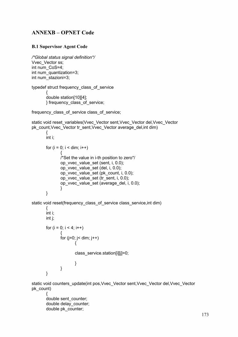
173

ANNEXB – OPNET Code

B.1 Supervisor Agent Code

/*Global status signal definition*/ Vvec_Vector ss; int num_CoS=4; int num_quantization=3; int num_stazioni=3;

typedef struct frequency_class_of_service { double station[10][4]; } frequency_class_of_service;

frequency_class_of_service class_of_service; static void reset_variables(Vvec_Vector sent,Vvec_Vector del,Vvec_Vector pk_count,Vvec_Vector tr_sent,Vvec_Vector average_del,int dim) { int i; for (i = 0; i < dim; i++) { /*Set the value in i-th position to zero*/ op_vvec_value_set (sent, i, 0.0); op_vvec_value_set (del, i, 0.0); op_vvec_value_set (pk_count, i, 0.0); op_vvec_value_set (tr_sent, i, 0.0); op_vvec_value_set (average_del, i, 0.0); } }

static void reset(frequency_class_of_service class_service,int dim) { int i; int j;

for (i = 0; i < 4; i++) { for (j=0; j< dim; j++) { class_service.station[i][j]=0; } } } static void counters_update(int pos,Vvec_Vector sent,Vvec_Vector del,Vvec_Vector pk_count) { double sent_counter; double delay_counter; double pk_counter;

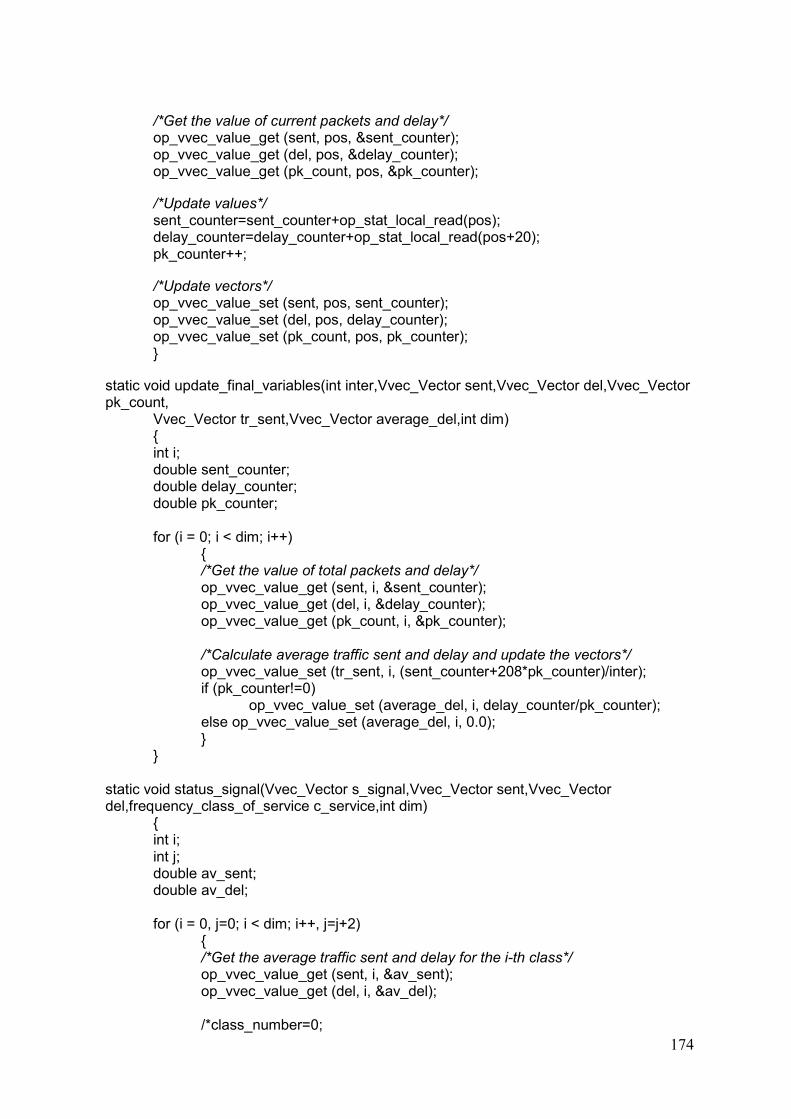
174

/*Get the value of current packets and delay*/ op_vvec_value_get (sent, pos, &sent_counter); op_vvec_value_get (del, pos, &delay_counter); op_vvec_value_get (pk_count, pos, &pk_counter);

/*Update values*/ sent_counter=sent_counter+op_stat_local_read(pos); delay_counter=delay_counter+op_stat_local_read(pos+20); pk_counter++;

/*Update vectors*/ op_vvec_value_set (sent, pos, sent_counter); op_vvec_value_set (del, pos, delay_counter); op_vvec_value_set (pk_count, pos, pk_counter); }

static void update_final_variables(int inter,Vvec_Vector sent,Vvec_Vector del,Vvec_Vector pk_count, Vvec_Vector tr_sent,Vvec_Vector average_del,int dim) { int i; double sent_counter; double delay_counter; double pk_counter; for (i = 0; i < dim; i++) { /*Get the value of total packets and delay*/ op_vvec_value_get (sent, i, &sent_counter); op_vvec_value_get (del, i, &delay_counter); op_vvec_value_get (pk_count, i, &pk_counter); /*Calculate average traffic sent and delay and update the vectors*/ op_vvec_value_set (tr_sent, i, (sent_counter+208*pk_counter)/inter); if (pk_counter!=0) op_vvec_value_set (average_del, i, delay_counter/pk_counter); else op_vvec_value_set (average_del, i, 0.0); } } static void status_signal(Vvec_Vector s_signal,Vvec_Vector sent,Vvec_Vector del,frequency_class_of_service c_service,int dim) { int i; int j; double av_sent; double av_del; for (i = 0, j=0; i < dim; i++, j=j+2) { /*Get the average traffic sent and delay for the i-th class*/ op_vvec_value_get (sent, i, &av_sent); op_vvec_value_get (del, i, &av_del); /*class_number=0;

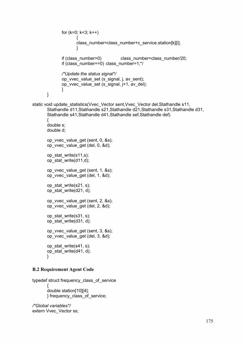
175

for (k=0; k<3; k++) { class_number=class_number+c_service.station[k][i]; } if (class_number>0) class_number=class_number/20; if (class_number==0) class_number=1;*/ /*Update the status signal*/ op_vvec_value_set (s_signal, j, av_sent); op_vvec_value_set (s_signal, j+1, av_del); } }

static void update_statistics(Vvec_Vector sent,Vvec_Vector del,Stathandle s11, Stathandle d11,Stathandle s21,Stathandle d21,Stathandle s31,Stathandle d31, Stathandle s41,Stathandle d41,Stathandle sef,Stathandle def) { double s; double d;

op_vvec_value_get (sent, 0, &s); op_vvec_value_get (del, 0, &d);

op_stat_write(s11,s); op_stat_write(d11,d);


op_stat_write(s21, s); op_stat_write(d21, d); op_vvec_value_get (sent, 2, &s); op_vvec_value_get (del, 2, &d);

op_stat_write(s31, s); op_stat_write(d31, d);


op_stat_write(s41, s); op_stat_write(d41, d); }

B.2 Requirement Agent Code

typedef struct frequency_class_of_service { double station[10][4]; } frequency_class_of_service;

/*Global variables*/ extern Vvec_Vector ss;

176

extern Vvec_Vector link_availability; extern frequency_class_of_service class_of_service; extern int num_CoS; extern int num_quantization; extern int num_stazioni;

/*Matrix of comparison (each row is a comparison vector, associated to a service class)*/ typedef Vvec_Vector Comparison_Supervisor [13]; typedef Vvec_Vector Q_values_matrix [243]; static double max_r(int state, Vvec_Vector super_state, Q_values_matrix Q, int CoS, int quantization);

static void reset_vector_zero (Vvec_Vector comp, int dimension) { int i; for (i=0; i<dimension; i++) { op_vvec_value_set (comp, i, 0); } }

static void init (Vvec_Vector Q, int dimension, double value) { int i; /*Initialize the elements of Q matrix with 'value'*/ for (i=0; i<dimension; i++) { op_vvec_value_set (Q, i, value); } }

static void reset_Q (Q_values_matrix Q, double r, int quantization, int CoS) { int i; /*Initialize the elements of Q matrix with 'value' The initialization proceeds from the first to the last row of Q matrix*/ for (i=0; i<pow(quantization, CoS+1); i++) { Q[i]=op_vvec_create(OpC_Type_Double); init(Q[i],CoS,r); } }

static void reset_learning_rate (Vvec_Vector l_rate, int quantization, int CoS) { int i; for (i=0; i<pow(quantization, CoS); i++) { op_vvec_value_set(l_rate, i, 1.0); } }

177

static void get_QoE (Vvec_Vector comp,double tr_adm, double av_delay,double min_tr,double max_del,double* lk_av) { /*Compute QoE 0*/ if (tr_adm>=min_tr && av_delay<=max_del) *lk_av=1;

else if (tr_adm>=min_tr && av_delay>max_del) *lk_av=0.5+0.5*(1-((av_delay-max_del)/max_del));

else if (tr_adm<min_tr && av_delay<=max_del) *lk_av=0.5+0.5*(1-((min_tr-tr_adm)/min_tr));

else if (tr_adm<min_tr && av_delay>max_del) *lk_av=0.5*(1-((min_tr-tr_adm)/min_tr))+0.5*(1-((av_delay-max_del)/max_del)); } static void get_QoE_super (Comparison_Supervisor comp, Vvec_Vector ind,Vvec_Vector s_signal,double min_tr,double max_del, Vvec_Vector lk_av_super, int dimension, frequency_class_of_service c_service, int num) { int i; int j; int k; double tr_sent; double av_del; double lk_av; double ind_super; double class_number;

/*For each row of the matrix comparison we compute the QoE*/ for (i=0, j=0; i<dimension; i++, j=j+2) { op_vvec_value_get (s_signal, j, &tr_sent); op_vvec_value_get (s_signal, j+1, &av_del); /*If the i-th service class doesn't send packets than it is free*/ if (tr_sent==0) op_vvec_value_set (lk_av_super, i, 1.0); else { /*Assign to local variable the QoE*/ op_vvec_value_get (lk_av_super, i, &lk_av); class_number=0; for (k=0; k<num; k++) { class_number=class_number+c_service.station[k][i]; } if (class_number>0) class_number=class_number/19; if (class_number==0) class_number=1;

178

tr_sent=tr_sent/class_number; /*Compute QoE for the i-th service class*/ get_QoE (comp[i],tr_sent,av_del,min_tr,max_del,&lk_av); /*Update QoE*/ op_vvec_value_set (lk_av_super, i, lk_av); } } } static void compute_agent_state(double lk_av, int* state, int quantization) { double lk_av_100; /*Compute the agent state from QoE*/ lk_av_100=lk_av*100; /*A quantization is introduced that divides the interval [0;1] into a finite set of sub-intervals*/ if (lk_av_100<=100) *state=2; if (lk_av_100<=90) *state=1; if (lk_av_100<=30) *state=0; } static void compute_ss_state(Vvec_Vector lk_av_super, Vvec_Vector s_state, int CoS, int quantization) { int i; double lk_av; int state; /*Compute the state of each Class of Service, from the status signal*/ for (i=0; i<CoS; i++) { op_vvec_value_get(lk_av_super, i, &lk_av); op_vvec_value_get(s_state, i, &state); compute_agent_state(lk_av, &state, quantization); op_vvec_value_set(s_state, i, state); } }

static void compute_reward(double lk_av, double lk_av_target, double *r) { /*Compute the reward of the agent*/ *r=-1000*(lk_av-lk_av_target)*(lk_av-lk_av_target); }

static void reinforcement_learning(int state_past, Vvec_Vector super_state_past, int act_past, int state, Vvec_Vector super_state, double r, Q_values_matrix Q, int CoS, int quantization, double alpha_0, double gamma)

179

{ int i; int s; int row; double q_val; double long_reward; /*From the global state of the agent (agent_state+supervisor_state) we compute the correspondent row of the Q_matrix (we consider the global state as a string of number expressed in base-val, with val equals to 'quantization')*/ row=0; for (i=0; i<CoS; i++) { op_vvec_value_get(super_state_past, i, &s); row=row+s*pow(quantization,i); } row=row+state_past*pow(quantization,CoS); /*Obtain the past value of the Q_matrix*/ op_vvec_value_get(Q[row], act_past, &q_val); /*Apply the Q_learning algorithm (past value+ increment)*/ long_reward=max_r(state,super_state,Q,CoS,quantization); q_val=q_val+alpha_0*(r+gamma*long_reward-q_val); if (q_val<-1000) q_val=-1000; /*Write the new value*/ op_vvec_value_set(Q[row], act_past, q_val); } static void get_learning_rate(Vvec_Vector l_rate, Vvec_Vector super_state, int quantization, int CoS, double* alpha_0) { int i; int s; int row; double app; row=0; for (i=0; i<CoS; i++) { op_vvec_value_get(super_state, i, &s); row=row+s*pow(quantization,i); } op_vvec_value_get(l_rate, row, &app); *alpha_0=app; op_vvec_value_set(l_rate, row, 0.98*app); }

180

static double max_r(int state, Vvec_Vector super_state, Q_values_matrix Q, int CoS, int quantization) { int i; int s; int row; double max_reward; double app; /*From the global state of the agent (agent_state+supervisor_state) we compute the correspondent row of the Q_matrix (we consider the globalstateas a string of number expressed in base-val, with val equals to 'quantization')*/ row=0; for (i=0; i<CoS; i++) { op_vvec_value_get(super_state, i, &s); row=row+s*pow(quantization,i); } row=row+state*pow(quantization,CoS); /*Compute, for the current state, the higher possible reward*/ op_vvec_value_get(Q[row], 0, &max_reward); for (i=1; i<CoS; i++) { op_vvec_value_get(Q[row], i, &app); if (app>max_reward) max_reward=app; } return max_reward; } static void next_action(int* a, int state, Vvec_Vector super_state, Q_values_matrix Q, double eps, int CoS, int quantization, int ide) { int i; int s; int row; double max_reward; int greedy_action; double app; /*From the global state of the agent (agent_state+supervisor_state) we compute the correspondent row of the Q_matrix (we consider the global state as a string of number expressed in base-val, with val equals to 'quantization')*/ row=0; for (i=0; i<CoS; i++) { op_vvec_value_get(super_state, i, &s); row=row+s*pow(quantization,i); }

181

row=row+state*pow(quantization,CoS); /*Compute, for the current state, tha higher possible reward; the action associated with this reward is the greedy action*/ greedy_action=0; op_vvec_value_get(Q[row], greedy_action, &max_reward); for (i=1; i<CoS; i++) { op_vvec_value_get(Q[row], i, &app); if (app>max_reward) { max_reward=app; greedy_action=i; } }

/*With probability 'eps' we choose a random action*/ app=((double) (rand() % 1000 +1))/1000; if (app>=eps) *a=greedy_action; else *a=rand() % CoS; }

static void action_to_class (int a, int* c) {

/*This method translates the action into a value correspondent to a real Class of Service. This number will be written into the IP header of the packet*/ if (a==0) *c=40; if (a==1) *c=72; if (a==2) *c=104; if (a==3) *c=136; }

A Reinforcement Learning based Cognitive Approach for...

Documents

Transcript of A Reinforcement Learning based Cognitive Approach for...