A Real-Time Distributed Hash TableTao Qian, Frank Mueller

North Carolina State University, USAmueller@cs.ncsu.edu

Yufeng XinRENCI, UNC-CH, USA

yxin@renci.org

Abstract—Currently, the North American power grid uses acentralized system to monitor and control wide-area power gridstates. This centralized architecture is becoming a bottleneck aslarge numbers of wind and photo-voltaic (PV) generation sourcesrequire real-time monitoring and actuation to ensure sustainedreliability. We have designed and implemented a distributedstorage system, a real-time distributed hash table (DHT), tostore and retrieve this monitoring data as a real-time serviceto an upper layer decentralized control system. Our real-timeDHT utilizes the DHT algorithm Chord in a cyclic executiveto schedule data-lookup jobs on distributed storage nodes.Weformally define the pattern of the workload on our real-time DHTand use queuing theory to stochastically derive the time boundfor response times of these lookup requests. We also define thequality of service (QoS) metrics of our real-time DHT as theprobability that deadlines of requests can be met. We use thestochastic model to derive the QoS. An experimental evaluation ondistributed nodes shows that our model is well suited to providetime bounds for requests following typical workload patternsand that a prioritized extension can increase the probability ofmeeting deadlines for subsequent requests.

I. I NTRODUCTION

The North American power grid uses Wide-Area MeasureSystem (WAMS) technology to monitor and control the stateof the power grid [17], [13]. WAMS increasingly relies onPhasor Measurement Units (PMUs), which are deployed todifferent geographic areas, e.g., the Eastern interconnectionarea, to collect real-time power monitoring data per area.These PMUs periodically send the monitored data to a phasordata concentrator (PDC) via proprietary Internet backbones.The PDC monitors and optionally controls the state of thepower grid on the basis of the data. However, the currentstate-of-the-art monitoring architecture uses one centralizedPDC to monitor all PMUs. As the number of PMUs isincreasing extremely fast nowadays, the centralized PDC willsoon become a bottleneck [5]. A straight-forward solution is todistribute multiple PDCs along with PMUs, where each PDCcollects real-time data from only the part of PMUs that thePDC is in charge of. In this way, the PDC is not the bottlenecksince the number of PMUs for each PDC could be limited andnew PDCs could be deployed to manage new PMUs.

New problems arise with such a distributed PDC architec-ture. In today’s power grid, real-time control actuation reliesin part on the grid states of multiple areas [16], but withthe new architecture the involved PMUs could be monitoredby different PDCs. The first problem is how to manage themapping between PDCs and PMUs so that a PDC can obtainPMU data from other PDCs. The second problem is how tocommunicate between these PDCs so that the real-time boundson control operation are still guaranteed. For simplification,we consider these PDCs as distributed storage nodes over awide-area network, where each of them periodically generates

This work was supported in part by NSF grants 1329780, 1239246, 0905181and 0958311. Aranya Chakrabortty helped to scope the problem in discussions.

records as long as the PDC periodically collects data fromthe PMUs in that area. Then, the problem becomes how toobtain these records from the distributed storage system withreal-time bounded response times.

Our idea is to build a distributed hash table (DHT) on thesedistributed storage nodes to solve the first problem. Similarto a single node hash table, a DHT providesput(key, value)and get(key)API services to upper layer applications. In ourDHT, the data of one PMU are not only stored in the PDC thatmanages the PMU, but also in other PDCs that keep redundantcopies according to the distribution resulting from the hashfunction and redundancy strategy. DHTs are well suited forthis problem due to their superior scalability, reliability, andperformance over centralized or even tree-based hierarchicalapproaches. The performance of the service provided by someDHT algorithms, e.g., Chord [15] and CAN [18], decreasesonly insignificantly while the number of the nodes in anoverlay network increases. However, there is a lack of researchon real-time bounds for these DHT algorithms for end-to-end response times of requests. Timing analysis is the key tosolve the second problem. On the basis of analysis, we couldprovide statistical upper bounds for request times. Without lossof generality, we use the termlookup requestor requesttorepresent either aput requestor a get request, since the corefunctionality of DHT algorithms is to look up the node that isresponsible for storing data associated with a given key.

It is difficult to analyze the time to serve a requestwithout prior information of the workloads on the nodes inthe DHT overlay network. In our research, requests followa certain pattern, which makes the analysis concrete. Forexample, PMUs periodically send real-time data to PDCs [13]so that PDCs issue put requests periodically. At the same time,PDCs need to fetch data from other PDCs to monitor globalpower states and control the state of the entire power gridperiodically. Using these patterns of requests, we design areal-time model to describe the system. Our problem is motivatedby power grid monitoring but our abstract real-time modelprovides a generic solution to analyze response times for real-time applications over networks. We further apply queuingtheory to stochastically analyze the time bounds for requests.Stochastic approaches may break with traditional views of real-time systems. However, cyber-physical systems rely on stockEthernet networks with enhanced TCP/IP so that soft real-timemodels for different QoS notions, such as simplex models [4],[1], are warranted.

Contributions : We have designed and implemented a real-time DHT by enhancing the Chord algorithm. Since a sequenceof nodes on the Chord overlay network serve a lookup request,each node is required to execute one corresponding job. Ourreal-time DHT follows a cyclic executive [11], [2] to schedulethese jobs on each node. We analyze the response time of thesesub-request jobs on each node and aggregate them to boundthe end-to-end response time for all requests. We also use a

stochastic model to derive the probability that our real-timeDHT can guarantee deadlines of requests. We issue a requestpattern according to the needs of real-time distributed storagesystems, e.g., power grid systems, on a cluster of workstationsto evaluate our model. In general, we present a methodologyfor analyzing the real-time response time of requests servedby multiple nodes on a network. This methodology includes:1) employing real-time executives on nodes, 2) abstractingapattern of requests, and 3) using a stochastic model to analyzeresponse time bounds under the cyclic executive and the givenrequest pattern. The real-time executive is not limited to acyclic executive. For example, we show that a prioritizedextension can increase the probability of meeting deadlinesfor requests that have failed during their first execution. Thiswork, while originally motivated by novel control methods inthe power grid, generically applies to distributed controlofCPS real-time applications.

The rest of the paper is organized as follows. Section IIpresents the design and implementation details of our real-time DHT. Section III presents our timing analysis and qualityof service model. Section IV presents the evaluation results.Section V presents the related work. Section VI presents theconclusion and the on-going part of our research.

II. D ESIGN AND IMPLEMENTATION

Our real-time DHT uses the Chord algorithm to locate thenode that stores a given data item. Let us first summarize theChord algorithm and characterize the lookup request pattern(generically and specifically for PMU data requests). Afterthat, we explain how our DHT implementation uses Chordand cyclic executives to serve these requests.

A. Chord

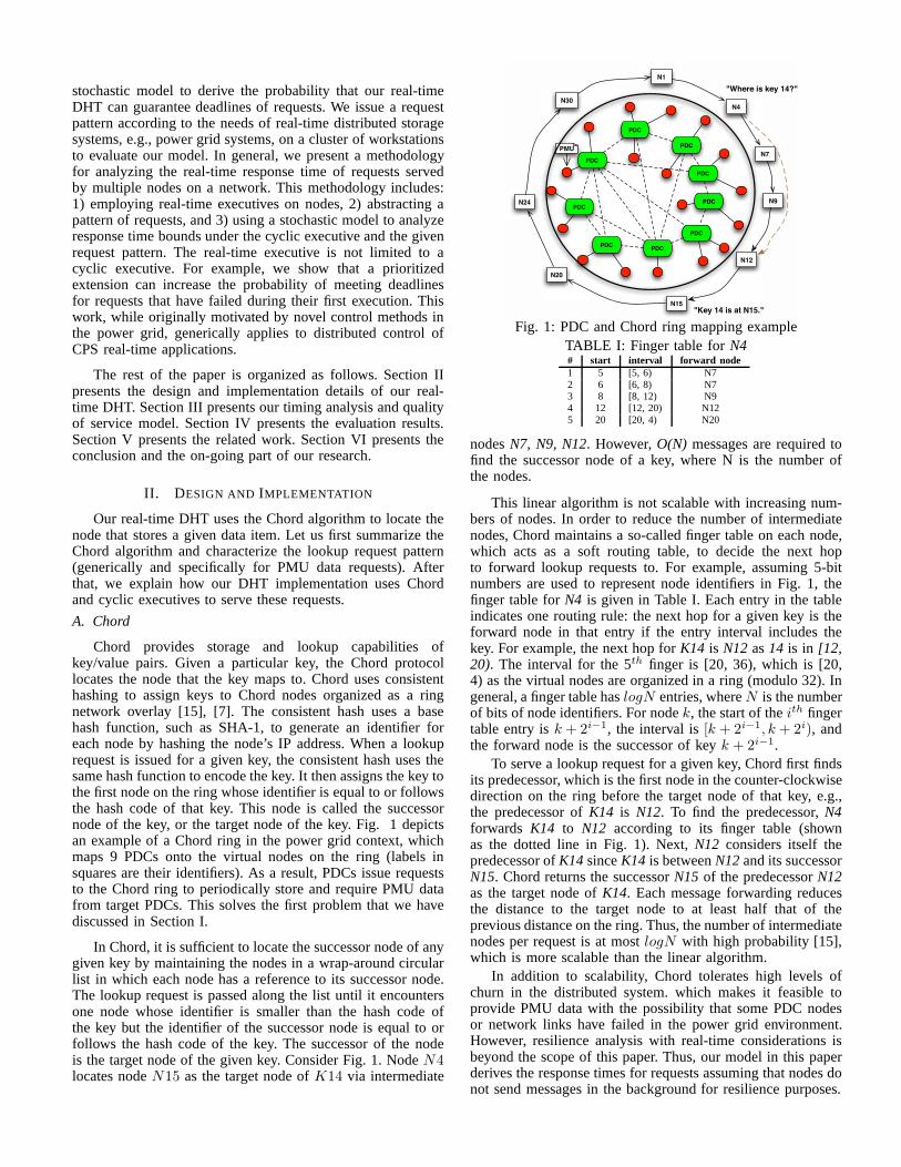
Chord provides storage and lookup capabilities ofkey/value pairs. Given a particular key, the Chord protocollocates the node that the key maps to. Chord uses consistenthashing to assign keys to Chord nodes organized as a ringnetwork overlay [15], [7]. The consistent hash uses a basehash function, such as SHA-1, to generate an identifier foreach node by hashing the node’s IP address. When a lookuprequest is issued for a given key, the consistent hash uses thesame hash function to encode the key. It then assigns the key tothe first node on the ring whose identifier is equal to or followsthe hash code of that key. This node is called the successornode of the key, or the target node of the key. Fig. 1 depictsan example of a Chord ring in the power grid context, whichmaps 9 PDCs onto the virtual nodes on the ring (labels insquares are their identifiers). As a result, PDCs issue requeststo the Chord ring to periodically store and require PMU datafrom target PDCs. This solves the first problem that we havediscussed in Section I.

In Chord, it is sufficient to locate the successor node of anygiven key by maintaining the nodes in a wrap-around circularlist in which each node has a reference to its successor node.The lookup request is passed along the list until it encountersone node whose identifier is smaller than the hash code ofthe key but the identifier of the successor node is equal to orfollows the hash code of the key. The successor of the nodeis the target node of the given key. Consider Fig. 1. NodeN4locates nodeN15 as the target node ofK14 via intermediate

PDC

PDC

PDC

PDCPDC

PMU

PDC

PDC

PDC

PDC

N4

N1

N7

N9

N12

N15

N20

N24

N30

"Where is key 14?"

"Key 14 is at N15."

Fig. 1: PDC and Chord ring mapping exampleTABLE I: Finger table forN4# start interval forward node1 5 [5, 6) N72 6 [6, 8) N73 8 [8, 12) N94 12 [12, 20) N125 20 [20, 4) N20

nodesN7, N9, N12. However,O(N) messages are required tofind the successor node of a key, where N is the number ofthe nodes.

This linear algorithm is not scalable with increasing num-bers of nodes. In order to reduce the number of intermediatenodes, Chord maintains a so-called finger table on each node,which acts as a soft routing table, to decide the next hopto forward lookup requests to. For example, assuming 5-bitnumbers are used to represent node identifiers in Fig. 1, thefinger table forN4 is given in Table I. Each entry in the tableindicates one routing rule: the next hop for a given key is theforward node in that entry if the entry interval includes thekey. For example, the next hop forK14 is N12 as14 is in [12,20). The interval for the 5th finger is [20, 36), which is [20,4) as the virtual nodes are organized in a ring (modulo 32). Ingeneral, a finger table haslogN entries, whereN is the numberof bits of node identifiers. For nodek, the start of theith fingertable entry isk + 2i−1, the interval is[k + 2i−1, k + 2i), andthe forward node is the successor of keyk + 2i−1.

To serve a lookup request for a given key, Chord first findsits predecessor, which is the first node in the counter-clockwisedirection on the ring before the target node of that key, e.g.,the predecessor ofK14 is N12. To find the predecessor,N4forwards K14 to N12 according to its finger table (shownas the dotted line in Fig. 1). Next,N12 considers itself thepredecessor ofK14sinceK14 is betweenN12and its successorN15. Chord returns the successorN15 of the predecessorN12as the target node ofK14. Each message forwarding reducesthe distance to the target node to at least half that of theprevious distance on the ring. Thus, the number of intermediatenodes per request is at mostlogN with high probability [15],which is more scalable than the linear algorithm.

In addition to scalability, Chord tolerates high levels ofchurn in the distributed system. which makes it feasible toprovide PMU data with the possibility that some PDC nodesor network links have failed in the power grid environment.However, resilience analysis with real-time considerations isbeyond the scope of this paper. Thus, our model in this paperderives the response times for requests assuming that nodesdonot send messages in the background for resilience purposes.

B. The pattern of requests and jobs

To eventually serve a request, a sequence of nodes areinvolved. The node that issues a request is called the initialnode of the request, and other nodes are called subsequentnodes. In the previous example,N4 is the initial node;N12,N15 are subsequent nodes. As stated in Section I, requests inthe power grid system follow a certain periodic pattern, whichmakes timing analysis feasible. In detail, each node in thesystem maintains a list of get and put tasks together with theperiod of each task. Each node releases periodic tasks in thelist to issue lookup requests. Once a request is issued, one jobon each node on the way is required to be executed until therequest is eventually served.

Jobs on the initial nodes are periodic, since they areinitiated by periodic real-time tasks. However, jobs on thesubsequent nodes are not necessarily periodic, since they aredriven by the lookup messages sent by other nodes via thenetwork. The network delay to transmit packets is not alwaysconstant, even through one packet is enough to forward arequest message as the length of PMU data is small in thepower grid system. Thus, the pattern of these subsequent jobsdepends on the node-to-node network delay. With differentconditions of the network delay, we consider two models.

(1) In the first model, the network delay to transmit alookup message is constant. Under this assumption, we use pe-riodic tasks to handle messages sent by other nodes. For exam-ple, assume node A has a periodic PUT taskτ1(0, T1, C1, D1).We use the notationτ(φ, T, C, D) to specify a periodic taskτ , whereφ is its phase,T is the period,C is the worst caseexecution time per job, andD is the relative deadline. Fromthe schedule table for the cyclic executive, the response timesfor the jobs ofτ1 in a hyperperiodH are known [11]. Assumetwo jobs of this task,J1,1 andJ1,2, are in one hyperperiod onnode A, withR1,1 andR1,2 as their release times relative tothe beginning of the hyperperiod andW1,1 and W1,2 as theresponse times, respectively.

Let the network latency,δ, be constant. The subsequentmessage of the jobJ1,1 is sent to node B at timeR1,1+W1,1+δ. For a sequence of hyperperiods on node A, the jobs to handlethese subsequent messages on node B become a periodic taskτ2(R1,1 +W1,1 + δ, H, C2, D2). The period of the new task isH as one message ofJ1,1 is issued per hyperperiod. Similarly,jobs to handle the messages ofJ1,2 become another periodictask τ3(R1,2 + W1,2 + δ, H, C2, D2) on node B.

(2) In the second model, network delay may be variable,and its distribution can be measured. We use aperiodic jobsto handle subsequent messages. Our DHT employs a cyclicexecutive on each node to schedule the initial periodic jobsandsubsequent aperiodic jobs, as discussed in the next section.

We focus on the second model in this paper since thismodel reflects the networking properties of IP-based networkinfrastructure. This is also consistent with current trends incyber-physical systems to utilize stock Ethernet networkswithTCP/IP enhanced by soft real-time models for different QoSnotions, such as the simplex model [4], [1]. The purely periodicmodel is subject to future work as it requires special hardwareand protocols, such as static routing and TDMA to avoidcongestion, to guarantee constant network delay.

C. Job scheduling

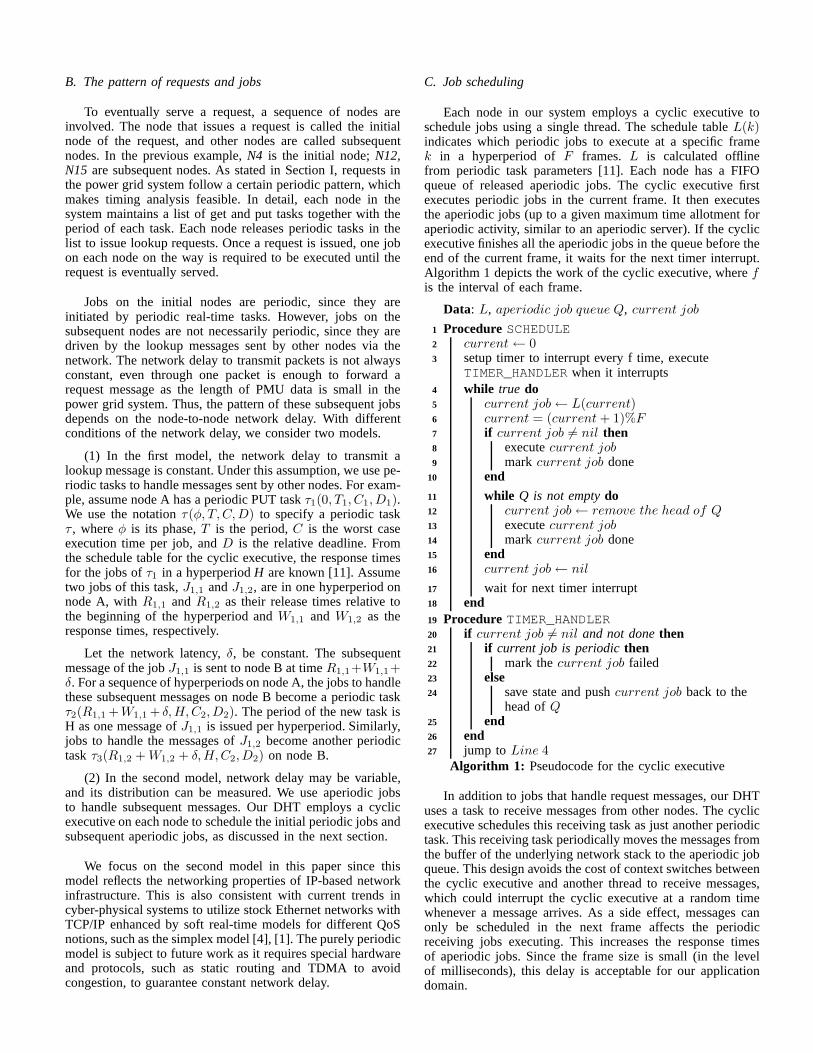
Each node in our system employs a cyclic executive toschedule jobs using a single thread. The schedule tableL(k)indicates which periodic jobs to execute at a specific framek in a hyperperiod ofF frames. L is calculated offlinefrom periodic task parameters [11]. Each node has a FIFOqueue of released aperiodic jobs. The cyclic executive firstexecutes periodic jobs in the current frame. It then executesthe aperiodic jobs (up to a given maximum time allotment foraperiodic activity, similar to an aperiodic server). If thecyclicexecutive finishes all the aperiodic jobs in the queue beforetheend of the current frame, it waits for the next timer interrupt.Algorithm 1 depicts the work of the cyclic executive, wherefis the interval of each frame.

Data: L, aperiodic job queue Q, current job

1 ProcedureSCHEDULE2 current← 03 setup timer to interrupt every f time, execute

TIMER_HANDLER when it interrupts4 while true do5 current job← L(current)6 current = (current + 1)%F7 if current job 6= nil then8 executecurrent job9 mark current job done

10 end

11 while Q is not emptydo12 current job← remove the head of Q13 executecurrent job14 mark current job done15 end16 current job← nil

17 wait for next timer interrupt18 end19 ProcedureTIMER_HANDLER20 if current job 6= nil and not donethen21 if current job is periodicthen22 mark thecurrent job failed23 else24 save state and pushcurrent job back to the

head ofQ25 end26 end27 jump to Line 4

Algorithm 1: Pseudocode for the cyclic executive

In addition to jobs that handle request messages, our DHTuses a task to receive messages from other nodes. The cyclicexecutive schedules this receiving task as just another periodictask. This receiving task periodically moves the messages fromthe buffer of the underlying network stack to the aperiodic jobqueue. This design avoids the cost of context switches betweenthe cyclic executive and another thread to receive messages,which could interrupt the cyclic executive at a random timewhenever a message arrives. As a side effect, messages canonly be scheduled in the next frame affects the periodicreceiving jobs executing. This increases the response timesof aperiodic jobs. Since the frame size is small (in the levelof milliseconds), this delay is acceptable for our applicationdomain.

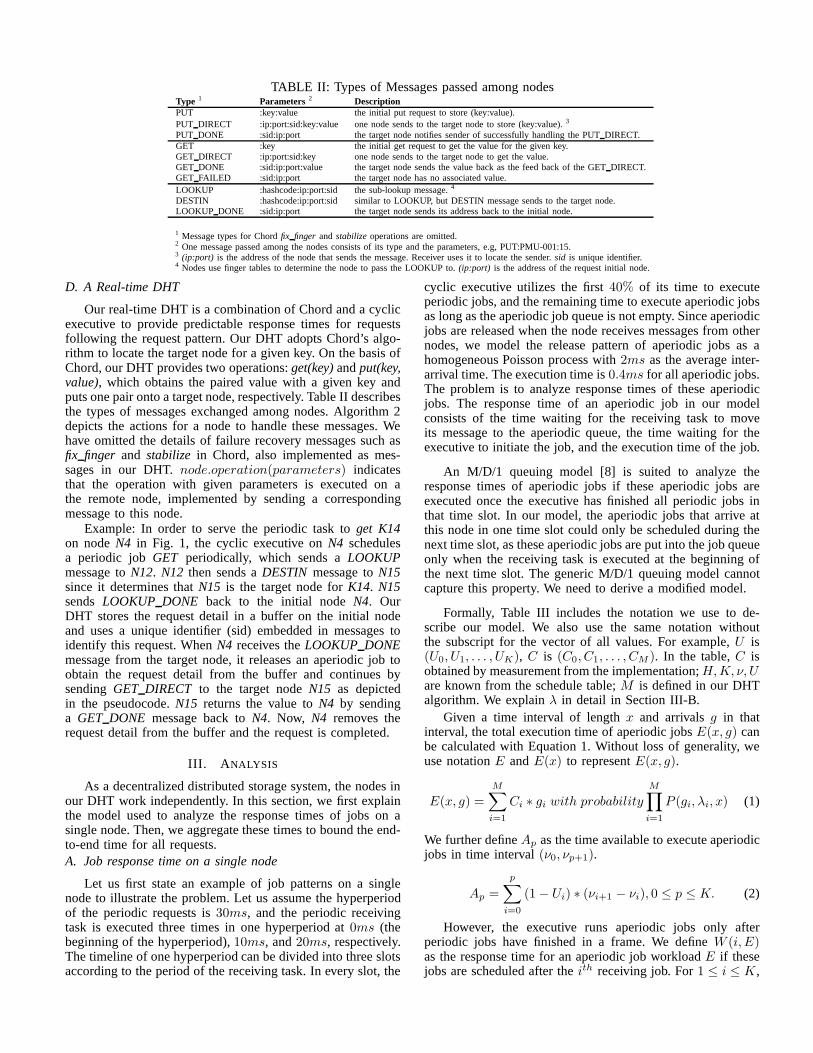
TABLE II: Types of Messages passed among nodesType 1 Parameters 2 DescriptionPUT :key:value the initial put request to store (key:value).PUT DIRECT :ip:port:sid:key:value one node sends to the targetnode to store (key:value).3

PUT DONE :sid:ip:port the target node notifies sender of successfully handling the PUTDIRECT.GET :key the initial get request to get the value for the givenkey.GET DIRECT :ip:port:sid:key one node sends to the target node toget the value.GET DONE :sid:ip:port:value the target node sends the value back as the feed back of the GETDIRECT.GET FAILED :sid:ip:port the target node has no associated value.LOOKUP :hashcode:ip:port:sid the sub-lookup message.4

DESTIN :hashcode:ip:port:sid similar to LOOKUP, but DESTIN message sends to the target node.LOOKUP DONE :sid:ip:port the target node sends its address back to the initial node.

1 Message types for Chordfix finger andstabilizeoperations are omitted.2 One message passed among the nodes consists of its type and the parameters, e.g, PUT:PMU-001:15.3 (ip:port) is the address of the node that sends the message. Receiver uses it to locate the sender.sid is unique identifier.4 Nodes use finger tables to determine the node to pass the LOOKUP to. (ip:port) is the address of the request initial node.

D. A Real-time DHT

Our real-time DHT is a combination of Chord and a cyclicexecutive to provide predictable response times for requestsfollowing the request pattern. Our DHT adopts Chord’s algo-rithm to locate the target node for a given key. On the basis ofChord, our DHT provides two operations:get(key)andput(key,value), which obtains the paired value with a given key andputs one pair onto a target node, respectively. Table II describesthe types of messages exchanged among nodes. Algorithm 2depicts the actions for a node to handle these messages. Wehave omitted the details of failure recovery messages such asfix finger and stabilize in Chord, also implemented as mes-sages in our DHT.node.operation(parameters) indicatesthat the operation with given parameters is executed on athe remote node, implemented by sending a correspondingmessage to this node.

Example: In order to serve the periodic task toget K14on nodeN4 in Fig. 1, the cyclic executive onN4 schedulesa periodic jobGET periodically, which sends aLOOKUPmessage toN12. N12 then sends aDESTIN message toN15since it determines thatN15 is the target node forK14. N15sendsLOOKUP DONE back to the initial nodeN4. OurDHT stores the request detail in a buffer on the initial nodeand uses a unique identifier (sid) embedded in messages toidentify this request. WhenN4 receives theLOOKUP DONEmessage from the target node, it releases an aperiodic job toobtain the request detail from the buffer and continues bysendingGET DIRECT to the target nodeN15 as depictedin the pseudocode.N15 returns the value toN4 by sendinga GET DONE message back toN4. Now, N4 removes therequest detail from the buffer and the request is completed.

III. A NALYSIS

As a decentralized distributed storage system, the nodes inour DHT work independently. In this section, we first explainthe model used to analyze the response times of jobs on asingle node. Then, we aggregate these times to bound the end-to-end time for all requests.A. Job response time on a single node

Let us first state an example of job patterns on a singlenode to illustrate the problem. Let us assume the hyperperiodof the periodic requests is30ms, and the periodic receivingtask is executed three times in one hyperperiod at0ms (thebeginning of the hyperperiod),10ms, and20ms, respectively.The timeline of one hyperperiod can be divided into three slotsaccording to the period of the receiving task. In every slot,the

cyclic executive utilizes the first40% of its time to executeperiodic jobs, and the remaining time to execute aperiodic jobsas long as the aperiodic job queue is not empty. Since aperiodicjobs are released when the node receives messages from othernodes, we model the release pattern of aperiodic jobs as ahomogeneous Poisson process with2ms as the average inter-arrival time. The execution time is0.4ms for all aperiodic jobs.The problem is to analyze response times of these aperiodicjobs. The response time of an aperiodic job in our modelconsists of the time waiting for the receiving task to moveits message to the aperiodic queue, the time waiting for theexecutive to initiate the job, and the execution time of the job.

An M/D/1 queuing model [8] is suited to analyze theresponse times of aperiodic jobs if these aperiodic jobs areexecuted once the executive has finished all periodic jobs inthat time slot. In our model, the aperiodic jobs that arrive atthis node in one time slot could only be scheduled during thenext time slot, as these aperiodic jobs are put into the job queueonly when the receiving task is executed at the beginning ofthe next time slot. The generic M/D/1 queuing model cannotcapture this property. We need to derive a modified model.

Formally, Table III includes the notation we use to de-scribe our model. We also use the same notation withoutthe subscript for the vector of all values. For example,U is(U0, U1, . . . , UK), C is (C0, C1, . . . , CM ). In the table,C isobtained by measurement from the implementation;H, K, ν, Uare known from the schedule table;M is defined in our DHTalgorithm. We explainλ in detail in Section III-B.

Given a time interval of lengthx and arrivalsg in thatinterval, the total execution time of aperiodic jobsE(x, g) canbe calculated with Equation 1. Without loss of generality, weuse notationE andE(x) to representE(x, g).

E(x, g) =

M∑

i=1

Ci ∗ gi with probability

M∏

i=1

P (gi, λi, x) (1)

We further defineAp as the time available to execute aperiodicjobs in time interval(ν0, νp+1).

Ap =

p∑

i=0

(1− Ui) ∗ (νi+1 − νi), 0 ≤ p ≤ K. (2)

However, the executive runs aperiodic jobs only afterperiodic jobs have finished in a frame. We defineW (i, E)as the response time for an aperiodic job workloadE if thesejobs are scheduled after theith receiving job. For1 ≤ i ≤ K,

1 ProcedureGET(key) and PUT(key, value)2 sid← unique request identifier3 code← hashcode(key)4 address← ip and port of this node5 store the request in the buffer6 executeLOOKUP(address, sid, code)

7 ProcedureLOOKUP(initial-node, sid, hashcode)8 next← next node for the lookup in the finger table9 if next = target node then

10 next.DESTIN(initial-node, sid, hashcode)11 else12 next.LOOKUP(initial-node, sid, hashcode)13 end

14 ProcedureDESTIN(initial-node, sid, hashcode)15 address← ip and port of this node16 initial-node.LOOKUP_DONE(address, sid)

17 ProcedureLOOKUP_DONE(target-node, sid)18 request← find buffered request using sid19 if request = get then20 target-node.GET_DIRECT(initial-node, sid,

request.key)21 else if request = put then22 target-node.PUT_DIRECT(initial-node, sid,

request.key, request.value)23 else if request = fix finger then24 update the finger table25 end

26 ProcedureGET_DIRECT(initial-node, sid, key)27 address← ip and port of this node28 value← find value forkey in local storage29 if value = nil then30 initial-node.GET_FAILED(address, sid)31 else32 initial-node.GET_DONE(address, sid, value)33 end

34 ProcedurePUT_DIRECT(initial-node, sid, key, value)35 address← ip and port of this node36 store the pair to local storage37 initial-node.PUT_DONE (address, sid)

38 ProcedurePUT_DONE, GET_DONE, GET_FAILED39 execute the associated operation

Algorithm 2: Pseudocode for message handling jobs

W (i, E) is a function ofE calculated from the schedule tablein three cases:

(1) If E ≤ Ai − Ai−1, which means the executive canuse the aperiodic job quota between(νi, νi+1] to finish theworkload, we can use the parameters of the periodic jobschedule in the schedule table to calculateW (i, E).

(2) If ∃p ∈ [i + 1, K] so thatE ∈ (Ap−1 − Ai−1, Ap −Ai−1], which means the executive utilizes all the aperiodic jobquota between(νi, νp) to execute the workload and finishesthe workload at a time between(νp, νp+1), thenW (i, E) =νp − νi + W (p, E −Ap−1 + Ai−1).

(3) In the last case, the workload is finished in the nexthyperperiod.W (i, E) becomesH−νi+W (0, E−AK+Ai−1).W (0, E) indicates that one can use the aperiodic quota beforethe first receiving job to execute the workload. If the first

TABLE III: NotationNotation MeaningH hyperperiodK number of receiving jobs in one hyperperiodνi time when theith receiving job is scheduled1,2

Ui utilization of periodic jobs in time interval(νi, νi+1)M number of different types of aperiodic jobsλi average arrival rate of theith type aperiodic jobsCi worst case execution time of theith type aperiodic jobsgi number of arrivals ofith aperiodic jobE(x, g) total execution time

for aperiodic jobs that arrive in time interval of lengthxW (i, E) response time for aperiodic jobs

if they are scheduled afterith receiving jobP (n, λ, x) probability of n arrivals in time interval of length x,

when arrival is a Poisson process with rateλ1 νi are relative to the beginning of the current hyperperiod.2 For convenience,ν0 is defined as the beginning of a hyperperiod,νK+1

is defined as the beginning of next hyperperiod.

receiving job is scheduled at the beginning of the hyperperiod,this value is the same asW (1, E). In addition, we require thatany workload finishes before the end of the next hyperperiod.This is accomplished by analyzing the timing of receivingjobs and ensures that the aperiodic job queue is in the samestate at the beginning of each hyperperiod, i.e., no workloadaccumulates from previous hyperperiods (except for the lasthyperperiod).

Let us assume an aperiodic jobJ of execution timeCm

arrives at timet relative to the beginning of the currenthyperperiod. Letp + 1 be the index of the receiving job suchthat t ∈ [νp, νp+1). We also assume that any aperiodic job thatarrives in this period is put into the aperiodic job queue bythis receiving job. Then, we derive the response time of thisjob in different cases.

(1) The periodic jobs that are left over from the previoushyperperiod and arrive beforeνp in the current frame cannotbe finished beforeνp+1. Equation 3 is the formal condition forthis case, in whichHLW is the leftover workload from theprevious hyperperiod.

HLW + E(νp)−Ap > 0 (3)

In this case, the executive has to first finish this leftoverworkload, then any aperiodic jobs that arrive in the timeperiod [νp, t), which is E(t − νp), before executing jobJ .As a result, the total response time of jobJ is the timeto wait for the next receiving job atνp+1, which puts Jinto the aperiodic queue, and the time to execute aperiodicthe job workloadLW (νp) + E(t − νp) + Cm, which isW (p+1, HLW+E(t)−Ap+Cm), after the(p+1)th receivingjob. The response time ofJ is expressed in Equation 4.

R(Cm, t) =(νp+1 − t) +W (p + 1, HLW + E(t)−Ap + Cm)

(4)

(2) In the second case, the periodic jobs that are left overfrom the previous hyperperiod and arrive beforeνp can befinished beforeνp+1; the formal condition and the responsetime are given by Equations 5 and 6, respectively.

HLW + E(νp) ≤ Ap (5)

R(Cm, t) = (νp+1 − t) + W (p + 1, E(t− νp) + Cm) (6)

The hyperperiod leftover workloadHLW is modeled asfollows. Consider three continuous hyperperiods,H1, H2, H3.The leftover workload fromH2 consists of two parts. The

first part,E(H − νK), is comprised of the aperiodic jobs thatarrive after the last receiving job inH2, as these jobs canonly be scheduled by the first receiving job inH3. The secondpart,E(H + νK)− 2AK+1, is the jobs that arrive inH1 andbefore the last receiving job inH2. These jobs have not beenscheduled during the entire aperiodic allotment overH1 andH2. We construct a distribution forHLW in this way. Inaddition, we can construct a series of distributions of HLW,where sequences of hyperperiods with different lengths areconsidered. This series converges (after three hyperperiods) toa distribution subsequently used as the overall HLW distribu-tion for this workload. However, our evaluation shows that twoprevious hyperperiods are sufficient for the request patterns.

This provides the stochastic modelR(Cm, t) for the re-sponse time of an aperiodic job of execution timeCm thatarrives at a specific timet. By samplingt in one hyperperiod,we have obtained the stochastic model for the response timeof aperiodic jobs that arrive at any time.B. End-to-end response time analysis

We aggregate the single node response times and networkdelays to transmit messages for the end-to-end response timeof requests. The response time of any request consists offour parts: (1) the response time of the initial periodic job— this value is known by the schedule table; (2) the totalresponse time of jobs to handle subsequent lookup messageson at mostlogN nodes with high probability [15], whereN is the number of nodes; (3) the response time of ape-riodic jobs to handle LOOKUPDONE, and the final pairof messages, e.g., PUTDIRECT and PUTDONE; (4) thetotal network delays to transmit these messages. We use avalueδ based on measurements for the network delay, whereP (network delay ≤ δ) ≥ T , for a given thresholdT .

To use the single node response time model, we need toknow the values of the model parameters of Table III. With theabove details on requests, we can obtainH, K, v, U from theschedule table.λ is defined as follows: letT be the periodof the initial request on each node, thenN

Tnew requests

arrive at our DHT in one time unit, and each request issuesat most logN subsequent lookup messages. Let us assumethat hash codes of nodes and keys are randomly located onthe Chord ring, which is of high probability with the SHA-1 hashing algorithm. Then each node receiveslogN

Tlookup

messages in one time unit. The arrival rate of LOOKUPand DESTIN messages islogN

T. In addition, each request

eventually generates one LOOKUPDONE message and onefinal pair of messages these messages, the arrive rate is1

T.

C. Quality of service

We define quality of service (QoS) as the probability thatour real-time DHT can guarantee requests to be finished beforetheir deadlines. Formally, given the relative deadlineD ofa request, we use the stochastic modelR(Cm, t) for singlenode response times and the aggregation model for end-to-endresponse times to derive the probability that the end-to-endresponse time of the request is equal to or less thanD. In thissection, we apply the formula of our model step by step toexplain how to derive this probability in practice.

The probability density functionρ(d, Cm) is defined asthe probability that the single node response time of a jobwith execution timeCm is d. We first derive the conditional

density functionρ(d, Cm|t), which is the probability under thecondition that the job arrives at timet, i.e., the probability thatR(Cm, t) = d. Then, we apply the law of total probability toderiveρ(d, Cm). The conditional density functionρ(d, Cm|t)is represented as a table of pairsπ(ρ, d), where ρ is theprobability that an aperiodic job finishes with response timed. We apply the algorithms described in Section III-A to buildthis table as follows. Letp + 1 be the index of the receivingjob such thatt ∈ [νp, νp+1).

(1) We need to know when to apply Equations 4 and6. This is determined by the probabilityχ that conditionHLW + E(νp, g) ≤ Ap holds. To calculateχ, we enumeratejob arrival vectorsg that have significant probabilities intime (0, νp) according to the Poisson distribution, and useEquation 1 to calculate the workloadE(νp, g) for each g.The term significant probability means any probability thatislarger than a given threshold, e.g.,0.0001%. Since the valuesof HLW and E(νp, g) are independent, the probability ofa specific pair ofHLW and arrival vectorg is given bysimply their product. As a result, we build a condition tableCT (g, ρ), in which each row represents a pair of vectorg,which consists of the numbers of aperiodic job arrivals in timeinterval (0, νp) under the conditionHLW + E(νp, g) ≤ Ap,and the corresponding probabilityρ for that arrival vector.Then,χ =

∑ρ is the total probability for that condition.

(2) We construct probability density tableπ2(ρ, d) forresponse times of aperiodic jobs under conditionHLW +E(νp) ≤ Ap. In this case, we enumerate job arrival vectorsgthat have significant probabilities in time(0, t− νp) accordingto the Poisson distribution. We use Equation 1 to calculate theirworkload and Equation 6 to calculate their response time foreachg. Each job arrival vector generates one row in densitytableπ2.

(3) We construct probability density tableπ3(ρ, d) forresponse times of aperiodic jobs under conditionHLW +E(νp) > Ap. We enumerate job arrival vectorsg that havesignificant probabilities in time(0, t) according to the Poissondistribution. We use Equation 4 to calculate response times.Since time interval(0, t) includes (0, νp), arrival vectorsthat are in condition tableCT must be excluded fromπ3,because rows inCT only represent arrivals that results inHLW + E(νp) ≤ Ap. We normalize the probabilities of theremaining rows. By normalizing, we mean multiplying eachprobability by a common constant factor, so that the sum ofthe probabilities is 1.

(4) We merge the rows in these two density tables to buildthe final table for the conditional density function. Beforemerging, we need to multiply every probability in tableπ2

by the weightχ, which indicates the probability that rows intable π2 are valid. For the same reason, every probability intableπ3 is multiplied by (1 − χ).

Now, we apply the law of total probability to deriveρ(d, Cm) from the conditional density functions by samplingt in [0, H). The conditional density tables for all samplesare merged into a final density table

∏(ρ, d). The samples

are uniformly distributed in[0, H) so that conditional densitytables have the same weight during the merge process. Afternormalization, table

∏is the single node response time density

function ρ(d, Cm).

We apply the aggregation rule described in Section III-Bto derive the end-to-end response time density function on the

1 ProcedureUNIQUE (π)2 πdes ← empty table3 for each row(ρ, d) in π do4 if row (ρold, d) exists inπdes then5 ρold ← ρold + ρ6 else7 add row(ρ, d) to πdes

8 end9 end

10 return πdes

11 ProcedureSUM (π1, π2)12 π3 ← empty table13 for each row(ρ1, d1) in π1 do14 for each row(ρ2, d2) in π2 do15 add row(ρ1 ∗ ρ2, d1 + d2) to π3

16 end17 end18 return UNIQUE(π3)

Algorithm 3: Density tables operations

basis ofρ(d, Cm). According to the rule, end-to-end responsetime includes the response time of the initial periodic job,network delays, and the total response time of(logN + 3)aperiodic jobs of different types. In order to represent thedensity function of the total response time for these aperiodicjobs, we define the operationSUM on two density tablesπ1

andπ2 as in Algorithm 3. The resulting density table has onerow (ρ1∗ρ2, d1+d2) for each pair of rows(ρ1, d1) and(ρ2, d2)from tableπ1 and π2, respectively. That is, each row in theresult represents one sum of two response times from the twotables and the probability of the aggregated response times.The density function of the total response time for(logN +3)aperiodic jobs is calculated as Equation 7 (SUM on all πi),whereπi is the density function for theith job.

ρ(d) =

logN+3∑

i=1

πi (7)

The maximum number of rows in density tableρ(d) is2(logN + 3)Hω, where2H is the maximum response timeof single node jobs, andω is the sample rate for arrival timet that we use to calculate each density table.

Let us return to the QoS metric, i.e., the probability thata request can be served within a given deadlineD. We firstreduceD by the fixed value∆, which includes the responsetime for the initial periodic job and network delays(logN +3)δ. Then, we aggregate rows in the density functionρ(d) tocalculate this probabilityP (D −∆).

P (D −∆) =∑

(ρi,di)∈ρ(d),di≤D−∆

ρi (8)

IV. EVALUATION

We evaluated our real-time DHT on a local cluster with2000 cores over 120 nodes. Each node features a 2-way SMPwith AMD Opteron 6128 (Magny Core) processors and 8cores per socket (16 cores per node). Each node has 32GBDRAM and Gigabit Ethernet (utilized in this study) as well asInfiniband Interconnect (not used here). We apply workloadsof different intensity according to the needs of the power

grid control system on different numbers of nodes (16 nodesare utilized in our experiments), which act like PDCs. Thenodes are not synchronized to each other relative to their startof hyperperiods as such synchronization would be hard tomaintain in a distributed system. We design experiments fordifferent intensity of workloads and then collect single-nodeand end-to-end response times of requests in each experiment.The intensity of a workload is quantified by the systemutilization under that workload. The utilization is determinedby the number of periodic lookup requests and other periodicpower control related computations. The lookup keys have lesseffect on the workload and statistic results as long as theyare evenly stored on the nodes, which has high probabilityin Chord. In addition, the utilization of aperiodic jobs isdetermined by the number of nodes in the system. The numberof messages passing between nodes increases logarithmicallywith the number of nodes, which results in an increase in thetotal number of aperiodic jobs. We compare the experimentalresults with the results given by our stochastic model for eachworkload.

In the third part of this section, we give experimentalresults of our extended real-time DHT, in which the cyclicexecutive schedules aperiodic jobs based on the prioritiesofrequests. The results show that most of the requests that havetight deadlines can be finished at the second trial under thecondition that the executive did not finish the request the firsttime around.

A. Low workloadIn this experiment, we implement workloads of low uti-

lizations as a cyclic executive schedule. A hyperperiod (30ms)contains three frames of 10ms, each with a periodic followedby an aperiodic set of jobs. The periodic jobs include thereceiving job for each frame and the following put/get jobs:In frame 1, each node schedules aput request followed bya get request; in frame 2 and 3, each node schedules aput request, respectively. In each frame, the cyclic executiveschedules acompute job once the periodic jobs in that framehave been executed. Thiscompute job is to simulate periodiccomputations on PDCs for power state estimation, which isimplemented as a tight loop of computation in our experiments.As a result, the utilizations of periodic jobs in the three framesare all40%. Any put/get requests forwarded to other nodes inthe DHT result in aperiodic (remote) jobs. The execution timeof aperiodic jobs is0.4ms. The system utilization is66.7%(40% for periodic jobs and26.7% for aperiodic jobs) whenthe workload is run with 4 DHT nodes.

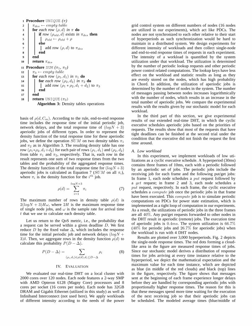
Results are plotted over 3,000 hyperperiods. Fig. 2 depictsthe single-node response times. The red dots forming a cloud-like area in the figure are measured response times of jobs.Since our stochastic model derives a distribution of responsetimes for jobs arriving at every time instance relative to thehyperperiod, we depict the mathematical expectation and themaximum value for each time instance, which are depictedas blue (in middle of the red clouds) and black (top) linesin the figure, respectively. The figure shows that messagessent at the beginning of each frame experience longer delaysbefore they are handled by corresponding aperiodic jobs withproportionally higher response times. The reason for this isthat these messages spend more time waiting for the executionof the next receiving job so that their aperiodic jobs canbe scheduled. The modeled average times (blue/middle of

clouds) follow a proportionally decaying curve delimited bythe respective periodic workload of a frame (4ms) plus theframe size (10ms) as the upper bound (left side) and just theperiodic workload as the lower bound (right side). The figureshows that the measured times (red/clouds) closely match thiscurve as the average response time for most of the arrivaltimes.

Maximum modeled times have a more complex pattern.In the first frame, their response times are bounded by 18msfor the first 4ms followed by a nearly proportionally decayingcurve (22ms-18ms response time) over the course of the next6ms. The spike at 4ms is due to servicing requests that arrivedin the first 4ms, including those from the previous hyperperiod.Similar spikes between frames exist for the same reason,where their magnitude is given by the density of remainingaperiodic jobs and the length of the periodic workload, whichalso accounts for the near-proportional decay. This results inaperiodic jobs waiting two frames before they execute whenissued during the second part of each frame.

0

2

4

6

8

10

12

14

16

18

20

22

24

0 2 4 6 8 10 12 14 16 18 20 22 24 26 28 30

Res

pons

e T

ime

(ms)

Relative Arrival Time (ms)

MeasuredModeled Average

Modeled Max

Fig. 2: Low-workload single-node response times (4 nodes)Fig. 3 depicts the cumulative distributions of single-node

response times for aperiodic jobs. The figure shows that99.3%of the aperiodic jobs finish within the next frame after theyare released under this workload, i.e., their response timesare bounded by14.4ms. Our model predicts that97.8% ofaperiodic jobs finish within the14.4ms deadline, which is agood match. In addition, for most of the response times in thefigure, our model predicts that a smaller fraction of aperiodicjobs finish within the response times than the fraction in theexperimental data as the blue (lower/solid) curve for modeledresponse times is below the red (upper/dashed) curve, i.e.,theformer effectively provides a lower bound for the latter. Thisindicates that our model is conservative for low workloads.

0

5

10

15

20

25

30

35

40

45

50

55

60

65

70

75

80

85

90

95

100

0 2 4 6 8 10 12 14 16 18 20

Cum

ulat

ive

Dis

trib

utio

n F

unct

ion

Response Time (ms)

Modeled AverageMeasured

Fig. 3: Low-workload single-node resp. times distr. (4 nodes)Fig. 4 depicts the cumulative distributions of end-to-end

response times for requests (left/right two lines for 4/8 nodes),

0

5

10

15

20

25

30

35

40

45

50

55

60

65

70

75

80

85

90

95

100

20 30 40 50 60 70 80 90 100 110 120

Cum

ulat

ive

Dis

trib

utio

n F

unct

ion

Response Time (ms)

Modeled Average (4 nodes)Modeled Average (8 nodes)

Measured (4 nodes)Measured (8 nodes)

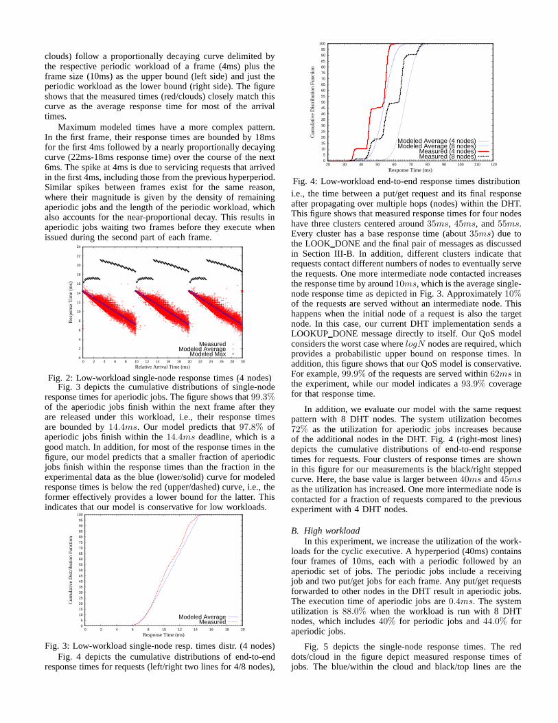
Fig. 4: Low-workload end-to-end response times distributioni.e., the time between a put/get request and its final responseafter propagating over multiple hops (nodes) within the DHT.This figure shows that measured response times for four nodeshave three clusters centered around35ms, 45ms, and55ms.Every cluster has a base response time (about35ms) due tothe LOOK DONE and the final pair of messages as discussedin Section III-B. In addition, different clusters indicatethatrequests contact different numbers of nodes to eventually servethe requests. One more intermediate node contacted increasesthe response time by around10ms, which is the average single-node response time as depicted in Fig. 3. Approximately10%of the requests are served without an intermediate node. Thishappens when the initial node of a request is also the targetnode. In this case, our current DHT implementation sends aLOOKUP DONE message directly to itself. Our QoS modelconsiders the worst case wherelogN nodes are required, whichprovides a probabilistic upper bound on response times. Inaddition, this figure shows that our QoS model is conservative.For example,99.9% of the requests are served within62ms inthe experiment, while our model indicates a93.9% coveragefor that response time.

In addition, we evaluate our model with the same requestpattern with 8 DHT nodes. The system utilization becomes72% as the utilization for aperiodic jobs increases becauseof the additional nodes in the DHT. Fig. 4 (right-most lines)depicts the cumulative distributions of end-to-end responsetimes for requests. Four clusters of response times are shownin this figure for our measurements is the black/right steppedcurve. Here, the base value is larger between40ms and45msas the utilization has increased. One more intermediate node iscontacted for a fraction of requests compared to the previousexperiment with 4 DHT nodes.

B. High workloadIn this experiment, we increase the utilization of the work-

loads for the cyclic executive. A hyperperiod (40ms) containsfour frames of 10ms, each with a periodic followed by anaperiodic set of jobs. The periodic jobs include a receivingjob and two put/get jobs for each frame. Any put/get requestsforwarded to other nodes in the DHT result in aperiodic jobs.The execution time of aperiodic jobs are0.4ms. The systemutilization is 88.0% when the workload is run with 8 DHTnodes, which includes40% for periodic jobs and44.0% foraperiodic jobs.

Fig. 5 depicts the single-node response times. The reddots/cloud in the figure depict measured response times ofjobs. The blue/within the cloud and black/top lines are the

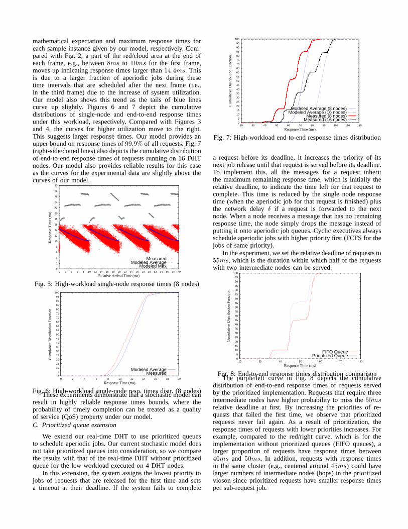
mathematical expectation and maximum response times foreach sample instance given by our model, respectively. Com-pared with Fig. 2, a part of the red/cloud area at the end ofeach frame, e.g., between8ms to 10ms for the first frame,moves up indicating response times larger than14.4ms. Thisis due to a larger fraction of aperiodic jobs during thesetime intervals that are scheduled after the next frame (i.e.,in the third frame) due to the increase of system utilization.Our model also shows this trend as the tails of blue linescurve up slightly. Figures 6 and 7 depict the cumulativedistributions of single-node and end-to-end response timesunder this workload, respectively. Compared with Figures 3and 4, the curves for higher utilization move to the right.This suggests larger response times. Our model provides anupper bound on response times of99.9% of all requests. Fig. 7(right-side/dotted lines) also depicts the cumulative distributionof end-to-end response times of requests running on 16 DHTnodes. Our model also provides reliable results for this caseas the curves for the experimental data are slightly above thecurves of our model.

0

2

4

6

8

10

12

14

16

18

20

22

24

26

28

30

0 2 4 6 8 10 12 14 16 18 20 22 24 26 28 30 32 34 36 38 40

Res

pons

e T

ime

(ms)

Relative Arrival Time (ms)

MeasuredModeled Average

Modeled Max

Fig. 5: High-workload single-node response times (8 nodes)

0

5

10

15

20

25

30

35

40

45

50

55

60

65

70

75

80

85

90

95

100

0 2 4 6 8 10 12 14 16 18 20

Cum

ulat

ive

Dis

trib

utio

n F

unct

ion

Response Time (ms)

Modeled AverageMeasured

Fig. 6: High-workload single-node resp. times distr. (8 nodes)These experiments demonstrate that a stochastic model can

result in highly reliable response times bounds, where theprobability of timely completion can be treated as a qualityof service (QoS) property under our model.C. Prioritized queue extension

We extend our real-time DHT to use prioritized queuesto schedule aperiodic jobs. Our current stochastic model doesnot take prioritized queues into consideration, so we comparethe results with that of the real-time DHT without prioritizedqueue for the low workload executed on 4 DHT nodes.

In this extension, the system assigns the lowest priority tojobs of requests that are released for the first time and setsa timeout at their deadline. If the system fails to complete

0

5

10

15

20

25

30

35

40

45

50

55

60

65

70

75

80

85

90

95

100

20 30 40 50 60 70 80 90 100 110 120

Cum

ulat

ive

Dis

trib

utio

n F

unct

ion

Response Time (ms)

Modeled Average (8 nodes)Modeled Average (16 nodes)

Measured (8 nodes)Measured (16 nodes)

Fig. 7: High-workload end-to-end response times distribution

a request before its deadline, it increases the priority of itsnext job release until that request is served before its deadline.To implement this, all the messages for a request inheritthe maximum remaining response time, which is initially therelative deadline, to indicate the time left for that request tocomplete. This time is reduced by the single node responsetime (when the aperiodic job for that request is finished) plusthe network delayδ if a request is forwarded to the nextnode. When a node receives a message that has no remainingresponse time, the node simply drops the message instead ofputting it onto aperiodic job queues. Cyclic executives alwaysschedule aperiodic jobs with higher priority first (FCFS forthejobs of same priority).

In the experiment, we set the relative deadline of requests to55ms, which is the duration within which half of the requestswith two intermediate nodes can be served.

0

5

10

15

20

25

30

35

40

45

50

55

60

65

70

75

80

85

90

95

100

20 30 40 50 60 70 80

Cum

ulat

ive

Dis

trib

utio

n F

unct

ion

Response Time (ms)

FIFO QueuePrioritized Queue

Fig. 8: End-to-end response times distribution comparisonThe purple/left curve in Fig. 8 depicts the cumulative

distribution of end-to-end response times of requests servedby the prioritized implementation. Requests that require threeintermediate nodes have higher probability to miss the55msrelative deadline at first. By increasing the priorities of re-quests that failed the first time, we observe that prioritizedrequests never fail again. As a result of prioritization, theresponse times of requests with lower priorities increases. Forexample, compared to the red/right curve, which is for theimplementation without prioritized queues (FIFO queues),alarger proportion of requests have response times between40ms and 50ms. In addition, requests with response timesin the same cluster (e.g., centered around45ms) could havelarger numbers of intermediate nodes (hops) in the prioritizedvioson since prioritized requests have smaller response timesper sub-request job.

V. RELATED WORK

Distributed hash tables are well known for their perfor-mance and scalability for looking up keys on a node that storesassociated values in a distributed environment. Many existingDHTs use the number of nodes involved in one lookup requestas a metric to measure performance. For example, Chordand Pastry requireO(logN) node traversals usingO(logN)routing tables to locate the target node for some data in anetwork ofN nodes [15], [19], while D1HT [14] and ZHT [10]requires a single node traversal at the expense ofO(N)routing tables. However, this level of performance analysisis not suited for real-time applications, as these applicationsrequire detailed timing information to guarantee time boundson lookup requests. In our research, we focus on analyzingresponse times of requests by modeling the pattern of jobexecutions on the nodes.

We build our real-time DHT on the basis of Chord. Eachnode maintains a small fraction of information of other nodesin its soft routing table. Compared with D1HT and ZHT, whereeach node maintains the information of all other nodes, Chordrequires less communication overhead to maintain its routingtable when nodes or links have failed in the DHT. Thus, webelieve a Chord-like DHT is more suitable for wide-area powergrid real-time state monitoring as it is more scalable in thenumbers of PDCs and PMUs.

In our timing analysis model, we assume that node-to-nodenetwork latency is bounded. Much of prior research changesthe OSI model to smooth packet streams so as to guaranteetime bounds on communication between nodes in switchedEthernet [9], [6]. Software-defined networks (SDN), whichallow administration to control traffic flows, are also suited tocontrol the network delay in a private network [12]. Distributedpower grid control nodes are spread in a wide area, but use aproprietary Internet backbone to communicate with each other.Thus, it is feasible to employ SDN technologies to guaranteenetwork delay bounds in a power grid environment [3].

VI. CONCLUSION

We have designed and implemented a real-time distributedhash table (DHT) on the basis of Chord to support a deadline-driven lookup service at upper layer control systems of theNorth American power grid. Our real-time DHT employs acyclic executive to schedule periodic and aperiodic lookupjobs. Furthermore, we formalize the pattern of a lookupworkload on our DHT according to the needs of power gridmonitoring and control systems, and use queuing theory toanalyze the stochastic bounds of response times for requestsunder that workload. We also derive the QoS model to measurethe probability that the deadlines of requests can be metby our real-time DHT. Our problem was motivated by thepower grid system but the cyclic executive and the approachof timing analysis generically applies to distributed storagesystems when requests follow our pattern. Our evaluationshows that our model is suited to provide an upper bound onresponse times and that a prioritized extension can increasethe probability of meeting deadlines for subsequent requests.

Our current analysis does not take node failures intoconsideration. With data replication (Chord stores data not onlyat the target node but in the nodes on the successor list [15]),requested data can still be obtained with high probability even

if node failures occur. Failures can be detected when jobs onone node fail to send messages to other nodes. In this case,the job searches the finger table again to determine the nextnode to send a data request message to, which increases theexecution times of that job. In future work, we will generalizeexecutions time modeling so that node failures are tolerated.

REFERENCES

[1] S. Bak, D.K. Chivukula, O. Adekunle, Mu Sun, M. Caccamo, andLui Sha. The system-level simplex architecture for improved real-timeembedded system safety. InIEEE Real-Time Embedded Technology andApplications Symposium, pages 99–107, 2009.

[2] T.P. Baker and Alan Shaw. The cyclic executive model and Ada.Technical Report 88-04-07, University of Washington, Department ofComputer Science, Seattle, Washington, 1988.

[3] A. Cahn, J. Hoyos, M. Hulse, and E. Keller. Software-defined energycommunication networks: From substation automation to future smartgrids. In IEEE Conf. on Smart Grid Communications, October 2013.

[4] T.L. Crenshaw, E. Gunter, C.L. Robinson, Lui Sha, and P.R. Kumar. Thesimplex reference model: Limiting fault-propagation due to unreliablecomponents in cyber-physical system architectures. InIEEE Real-TimeSystems Symposium, pages 400–412, 2007.

[5] J. E. Dagle. Data management issues associated with the august 14,2003 blackout investigation. InIEEE PES General Meeting - Panel onMajor Grid Blackouts of 2003 in North Akerica and Europe, 2004.

[6] J. D. Decotignie. Ethernet-based real-time and industrial communica-tions. Proceedings of the IEEE, 93(6):1102–1117, 2005.

[7] D. Karger, E. Lehman, T. Leighton, R. Panigrahy, M. Levine, andD. Lewin. Consistent hashing and random trees: Distributedcachingprotocols for relieving hot spots on the world wide web. InACMSymposium on Theory of Computing, pages 654–663, 1997.

[8] L. Kleinrock. Queueing systems. volume 1: Theory. 1975.

[9] S. K. Kweon and K. G. Shin. Achieving real-time communication overethernet with adaptive traffic smoothing. Inin Proceedings of RTAS2000, pages 90–100, 2000.

[10] Tonglin Li, Xiaobing Zhou, Kevin Brandstatter, Dongfang Zhao,Ke Wang, Anupam Rajendran, Zhao Zhang, and Ioan Raicu. Zht: Alight-weight reliable persistent dynamic scalable zero-hop distributedhash table. InParallel & Distributed Processing Symposium (IPDPS),2013.

[11] J. Liu. Real-Time Systems. Prentice Hall, 2000.

[12] N. McKeown. Software-defined networking. INFOCOM keynote talk,2009.

[13] W. A. Mittelstadt, P. E. Krause, P. N. Overholt, D. J. Sobajic, J. F. Hauer,R. E. Wilson, and D. T. Rizy. The doe wide area measurement system(wams) project demonstration of dynamic information technology forthe future power system. InEPRI Conference on the Future of PowerDelivery, 1996.

[14] L. Monnerat and C. Amorim. Peer-to-peer single hop distributed hashtables. Inin GLOBECOM’09, pages 1–8, 2009.

[15] Robert Morris, David Karger, Frans Kaashoek, and Hari Balakrishnan.Chord: A Scalable Peer-to-Peer Lookup Service for InternetApplica-tions. In ACM SIGCOMM 2001, San Diego, CA, September 2001.

[16] M. Parashar and J. Mo. Real time dynamics monitoring system:Phasor applications for the control room. In42nd Hawaii InternationalConference on System Sciences, pages 1–11, 2009.

[17] A. G. Phadke, J. S. Thorp, and M. G. Adamiak. New measurementtechniques for tracking voltage phasors, local system frequency, andrate of change of frequency.IEEE Transactions on Power Apparatusand Systems, 102:1025–1038, 1983.

[18] S. Ratnasamy, P. Francis, M. Handley, R. Karp, and S. Schenker.A scalable content-addressable network. Inin Proceedings of ACMSIGCOMM, pages 161–172, 2001.

[19] Antony I. T. Rowstron and Peter Druschel. Pastry: Scalable, decentral-ized object location, and routing for large-scale peer-to-peer systems.In Middleware ’01: Proceedings of the IFIP/ACM InternationalCon-ference on Distributed Systems Platforms Heidelberg, pages 329–350,London, UK, 2001. Springer-Verlag.