A Reactive Inelasticity Theoretical Framework for …...A Reactive Inelasticity Theoretical...

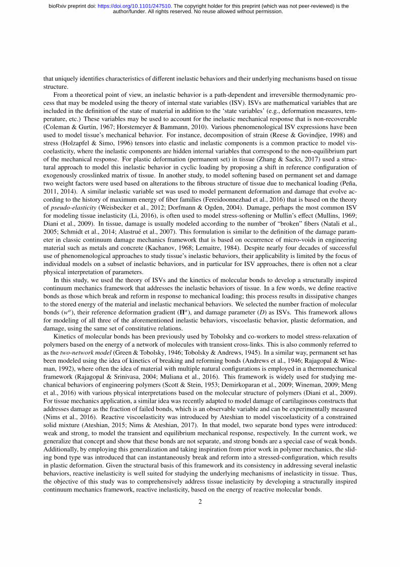
A Reactive Inelasticity Theoretical Framework for Modeling Viscoelasticity,Plastic Deformation, and Damage in Soft TissueI,II

Babak N. Safaa,b, Michael H. Santarea,b, Dawn M. Elliotta,b,1,∗

aDepartment of Mechanical Engineering, University of Delaware, Newark, DE, United StatesbDepartment of Biomedical Engineering, University of Delaware, Newark, DE, United States

Abstract

Soft tissues are biopolymeric materials, primarily made of collagen and water. These tissues have non-linear, anisotropic,and inelastic mechanical behaviors that are often categorized into viscoelastic behavior, plastic deformation, and dam-age. While tissue’s elastic and viscoelastic mechanical properties have been measured for decades, there is no com-prehensive theoretical framework for modeling inelastic behaviors of these tissues that is based on their structure. Tomodel the three major inelastic mechanical behaviors of soft tissue we formulated a structurally inspired continuummechanics framework based on the energy of molecular bonds that break and reform in response to external loading(reactive bonds). In this framework, we employed the theory of internal state variables and kinetics of molecularbonds. The number fraction of bonds, their reference deformation gradient, and damage parameter were used as in-ternal state variables that allowed for consistent modeling of all three of the inelastic behaviors of tissue by using thesame sets of constitutive relations. Several numerical examples are provided that address practical problems in tissuemechanics, including the difference between plastic deformation and damage. This model can be used to identifyrelationships between tissue’s mechanical response to external loading and its biopolymeric structure.

Keywords: Thermomechanical processes, Elastic-plastic material, Viscoelastic material, Damage, Soft tissue

1. Introduction

Soft tissues such as tendon, meniscus, intervertebral disc, etc., are biopolymeric material that have non-linear,anisotropic, and inelastic mechanical behaviors. An inelastic behavior, contrary to an elastic behavior, is one thatdissipates energy in a non-recoverable fashion. Three major inelastic behaviors that are experimentally observed insoft tissues are: viscoelastic behavior (Woo et al., 1980; Huang et al., 2001; Connizzo & Grodzinsky, 2017), plasticdeformation (Maher et al., 2012; Caro-Bretelle et al., 2015), and damage (Natali et al., 2005; Von Forell & Bowden,2014). Understanding the underlying mechanisms of these behaviors is essential for elucidating the relationshipsamong the mechanical loading, pathological conditions (e.g., tendinopathy, meniscus rupture, and disc herniation),and tissue’s structure.

Soft tissues have a hierarchical fibrous structure that is predominantly composed of collagen and water, where theunderlying microstructural organization is responsible for the variations in tissue’s mechanical properties. Inelasticmechanical responses can occur with loading, resulting in altered microstructure and mechanical properties, and evenloss of function and rupture. While tissue’s elastic and viscoelastic behaviors have been studied for decades, there is nocomprehensive framework for studying inelastic behaviors of tissue in a structural context; perhaps due to the complexnature of experimental measurement of the inelastic behaviors that occur simultaneously and can have overlappingeffects (e.g., plastic deformation and damage). Thus, a theoretical framework is necessary to study these behaviors

IThis document is a collaborative effort.IIFull length article. Word count: 8497∗Corresponding authorEmail address: [email protected] (Dawn M. Elliott)

1150 Academy Street, 161 Colburn Lab, Newark, DE 19716

Preprint submitted to bioRxiv repository January 18, 2018

author/funder. All rights reserved. No reuse allowed without permission. The copyright holder for this preprint (which was not peer-reviewed) is the. https://doi.org/10.1101/247510doi: bioRxiv preprint

https://doi.org/10.1101/247510

that uniquely identifies characteristics of different inelastic behaviors and their underlying mechanisms based on tissuestructure.

From a theoretical point of view, an inelastic behavior is a path-dependent and irreversible thermodynamic pro-cess that may be modeled using the theory of internal state variables (ISV). ISVs are mathematical variables that areincluded in the definition of the state of material in addition to the ‘state variables’ (e.g., deformation measures, tem-perature, etc.) These variables may be used to account for the inelastic mechanical response that is non-recoverable(Coleman & Gurtin, 1967; Horstemeyer & Bammann, 2010). Various phenomenological ISV expressions have beenused to model tissue’s mechanical behavior. For instance, decomposition of strain (Reese & Govindjee, 1998) andstress (Holzapfel & Simo, 1996) tensors into elastic and inelastic components is a common practice to model vis-coelasticity, where the inelastic components are hidden internal variables that correspond to the non-equilibrium partof the mechanical response. For plastic deformation (permanent set) in tissue (Zhang & Sacks, 2017) used a struc-tural approach to model this inelastic behavior in cyclic loading by proposing a shift in reference configuration ofexogenously crosslinked matrix of tissue. In another study, to model softening based on permanent set and damagetwo weight factors were used based on alterations to the fibrous structure of tissue due to mechanical loading (Pena,2011, 2014). A similar inelastic variable set was used to model permanent deformation and damage that evolve ac-cording to the history of maximum energy of fiber families (Fereidoonnezhad et al., 2016) that is based on the theoryof pseudo-elasticity (Weisbecker et al., 2012; Dorfmann & Ogden, 2004). Damage, perhaps the most common ISVfor modeling tissue inelasticity (Li, 2016), is often used to model stress-softening or Mullin’s effect (Mullins, 1969;Diani et al., 2009). In tissue, damage is usually modeled according to the number of “broken” fibers (Natali et al.,2005; Schmidt et al., 2014; Alastrue et al., 2007). This formulation is similar to the definition of the damage param-eter in classic continuum damage mechanics framework that is based on occurrence of micro-voids in engineeringmaterial such as metals and concrete (Kachanov, 1968; Lemaitre, 1984). Despite nearly four decades of successfuluse of phenomenological approaches to study tissue’s inelastic behaviors, their applicability is limited by the focus ofindividual models on a subset of inelastic behaviors, and in particular for ISV approaches, there is often not a clearphysical interpretation of parameters.

In this study, we used the theory of ISVs and the kinetics of molecular bonds to develop a structurally inspiredcontinuum mechanics framework that addresses the inelastic behaviors of tissue. In a few words, we define reactivebonds as those which break and reform in response to mechanical loading; this process results in dissipative changesto the stored energy of the material and inelastic mechanical behaviors. We selected the number fraction of molecularbonds (wα), their reference deformation gradient (Πα), and damage parameter (D) as ISVs. This framework allowsfor modeling of all three of the aforementioned inelastic behaviors, viscoelastic behavior, plastic deformation, anddamage, using the same set of constitutive relations.

Kinetics of molecular bonds has been previously used by Tobolsky and co-workers to model stress-relaxation ofpolymers based on the energy of a network of molecules with transient cross-links. This is also commonly referred toas the two-network model (Green & Tobolsky, 1946; Tobolsky & Andrews, 1945). In a similar way, permanent set hasbeen modeled using the idea of kinetics of breaking and reforming bonds (Andrews et al., 1946; Rajagopal & Wine-man, 1992), where often the idea of material with multiple natural configurations is employed in a thermomechanicalframework (Rajagopal & Srinivasa, 2004; Muliana et al., 2016). This framework is widely used for studying me-chanical behaviors of engineering polymers (Scott & Stein, 1953; Demirkoparan et al., 2009; Wineman, 2009; Menget al., 2016) with various physical interpretations based on the molecular structure of polymers (Diani et al., 2009).For tissue mechanics application, a similar idea was recently adapted to model damage of cartilaginous constructs thataddresses damage as the fraction of failed bonds, which is an observable variable and can be experimentally measured(Nims et al., 2016). Reactive viscoelasticity was introduced by Ateshian to model viscoelasticity of a constrainedsolid mixture (Ateshian, 2015; Nims & Ateshian, 2017). In that model, two separate bond types were introduced:weak and strong, to model the transient and equilibrium mechanical response, respectively. In the current work, wegeneralize that concept and show that these bonds are not separate, and strong bonds are a special case of weak bonds.Additionally, by employing this generalization and taking inspiration from prior work in polymer mechanics, the slid-ing bond type was introduced that can instantaneously break and reform into a stressed-configuration, which resultsin plastic deformation. Given the structural basis of this framework and its consistency in addressing several inelasticbehaviors, reactive inelasticity is well suited for studying the underlying mechanisms of inelasticity in tissue. Thus,the objective of this study was to comprehensively address tissue inelasticity by developing a structurally inspiredcontinuum mechanics framework, reactive inelasticity, based on the energy of reactive molecular bonds.

2


https://doi.org/10.1101/247510

This paper is organized as follows: in Section 2 we formulate the theory of reactive inelasticity by defining thefree energy of a reactive body with generic molecular bond types, where the concepts of intrinsic hyperelasticity andgeneralized bond kinetics are formulated. Further, we introduce special bond types suited for different mechanicalbehaviors: formative bonds for a viscoelastic behavior, permanent bonds for hyperelastic behavior, and sliding bondsfor plastic deformation. Damage is added to the formulation by allowing for the reduction of the number fraction ofload bearing bonds. To demonstrate the key features of this framework, in Section 3 we provide several numericalexamples of the mechanical behavior of single bond types and their combinations. Finally, in Section 4, comparisonsto the other existing inelasticity models for tissue, and physical interpretation of bonds are discussed.

2. Reactive inelasticity

In the following, we will describe the mechanics of a reactive material. In brief, a reactive material is madeof a combination of different bond types each with different characteristics. Each bond type is associated with acertain mechanical behavior (e.g., formative bonds with viscoelastic behavior). Bonds break and reform (i.e., react)when subjected to an external loading and this process initiates new generations. Generations are molecular bonds ofcertain bond type that were initiated at the same time and, thus, have a mutual reference configuration. By using thekinetics rate of bond breakage and formation, the states of energy and stress are determined. Damage is introducedto all of the bond types by reducing the fraction of active bonds in the material, and finally the consequences of thesecond law of thermodynamics are discussed.

2.1. Kinematics and relative deformationConsider a solid body made of a set of material points that are energetically constrained with different types of

molecular bonds (indicated by a subscript γ). These bonds deform in a smooth path x B χ(X, t), where x stands for thecurrent configuration of bonds and X is their master reference configuration. Hence, the deformation gradient tensoris defined as F B ∂χ(X,t)

∂X and the right Cauchy-Green deformation tensor as C B FT F. Each bond type may havedifferent generations (indicated by superscript α), and despite their mutual path of deformation and master referenceconfiguration, every generation has a different reference configuration (Xα

γ ), which is a function of the conditions atthe time of formation of the bonds (Fig. 1). By using the chain rule of differentiation, the relative deformation gradienttensor for each generation (Fα

γ ) isFαγ B F(Πα

γ )−1 , (2.1)

where Παγ B

∂Xαγ

∂X is the reference deformation gradient tensor of generation α of bond type γ. This procedure resultsin multiplicative decomposition of deformation (Lee, 1969; Simo, 1988; Lubarda, 2004). As a result, the relative rightCauchy-Green deformation tensor Cα

γ isCαγ B (Πα

γ )−T C(Παγ )−1 ; (2.2)

note that A−T := (A−1)T .

2.2. Free energy and intrinsic hyperelasticityThe free energy density of the system is the combination of the energy density of all the bond types

Ψ =∑γ

Ψγ , (2.3)

where Ψ is the Helmholtz free energy density (per volume). The energy density of each bond type is the sum of theenergy from each of its generations

Ψγ =∑α

nαγ ψαγ , (2.4)

where nαγ is the number density, and ψαγ is the average energy of bonds from generation α of bond type γ. Alternatively,by defining the number fraction of each generation as

wαγ =

nαγ∑α nαγ

=nαγ

nγ,total, (2.5)

3


https://doi.org/10.1101/247510

Master Reference

Configuration

Generation Reference

Configuration

Current Configuration

Figure 1. Reference configuration of generations: In a body with the master reference configuration X for generation α therelative deformation gradient tensor (Fα) is defined using the reference configuration (Xα).

where nγ,total is the number density of a bond type in the natural state of the material, Eq. (2.4) can be re-written as

Ψγ =∑α

wαγψ

αγ , (2.6)

whereψαγ = nγ,totalψ

αγ . (2.7)

Here, ψαγ denotes the overall energy density of a generation, which, in general, can be a function of deformation,temperature and other state variables. However, in this formulation we consider a unique deformation dependencethat implies that generations are intrinsically hyperelastic. That is,

ψαγ = ψγ(Cα) . (2.8)

The above equation also denotes that the intrinsic hyperelasticity relation is the same for all of the generations of onebond type, and thus is a characteristic of that type of bonds. Therefore, Eq. (2.6) reads as

Ψγ =∑α

wαγψγ(Cα

γ ) . (2.9)

Note that for a bond type with no damage ∑α

wαγ = 1 , (2.10)

which indicates that the energy density of each bond type (Eq. (2.9)) is a weighted sum of the energy density of all itsgenerations. Thus, the overall free energy density of the material can be written in the following form

Ψ(C,wαγ ,Π

αγ ) =

∑γ

∑α

wαγψγ(Cα

γ ) . (2.11)

Here, deformation (represented by C) is the only “state variable” and the number fraction of generations of bond types(wα

γ ) as well as their reference deformation gradient (Παγ ) are the “internal state variables (ISV)”. To simplify the

notation without losing generality, we will continue the discussion for one type of bond, where the total response fora mixture of multiple bond types should be taken as a summation over all existing bond types (such as in Eq. (2.11)).

The second Piola-Kirchhoff stress tensor is written as (Coleman & Gurtin, 1967)

S(C,wαγ ,Π

αγ ) = 2

∂Ψ(C,wαγ ,Π

αγ )

∂C. (2.12)

4


https://doi.org/10.1101/247510

Also, by using Eq. (2.9) for a reactive material, Eq. (2.12) can be re-written as (see Appendix A)

S(C,wα,Πα) =∑α

wα(Πα)−1Sα(Cα)(Πα)−T , (2.13)

where we also adopted the following definition for stress associated with each generation:

Sα(Cα) B 2∂ψ(Cα)∂Cα

. (2.14)

To enforce coordinate-invariance, the state of stress equivalently is determined using the invariants of Cα:

Iα1 = tr(Cα), Iα2 =12

[tr(Cα)2 − tr((Cα)2)

], and Iα3 = det(Cα) , (2.15)

where tr(.) and det(.) stand for trace and determinant of a second order tensor, respectively. In general, the given setof invariants suffices to define the state of deformation; however, it is customary to add additional pseudo invariantsfor anisotropic material (e.g., tendon, and ligament). A common pseudo invariant for transversely isotropic materialis defined as (Spencer, 1984; Cortes & Elliott, 2014)

Iα4 BMα : Cα , (2.16)

In this equation, Mα is a second-order structure tensor defined as

Mα B eαγ ⊗ eαγ , where eαγ BΠαe0

γ

||Παe0γ||. (2.17)

Here, eαγ is a unit vector on the dominant fiber direction in the generation α reference configuration. Therefore, thesecond Piola-Kirchhoff stress (S) in terms of deformation invariants reads as

S(C,wα,Πα) =∑α

wα(Πα)−1

4∑i=1

2∂ψ

∂Iαi

∂Iαi∂Cα

(Πα)−T , (2.18)

where the derivatives of the deformation invariants are∂Iα1∂Cα

= I,∂Iα2∂Cα

= Iα1 I − Cα,∂Iα3∂Cα

= Iα3 (Cα)−1, and∂Iα4∂Cα

= Mα . (2.19)

The Cauchy stress (T) is then obtained from the second Piola-Kirchhoff stress (Eq. (2.18)) as

T =1J

FSFT . (2.20)

By using the relative deformation gradient tensor, defined earlier in Eq. (2.1), the Cauchy stress tensor for each bondtype is

T(C,wα,Πα) =1J

∑α

wαFα

4∑i=1

2∂ψ

∂Iαi

∂Iαi∂Cα

(Fα)T , (2.21)

and by defining the contribution of each generation (Tα) as

Tα(Cα) B1J

Fα

4∑i=1

2∂ψ

∂Iαi

∂Iαi∂Cα

(Fα)T , (2.22)

the Cauchy stress tensor for a specific bond type reads as

T(C,wα,Πα) =∑α

wαTα(Cα) . (2.23)

Similar to energy, the above equation indicates that the Cauchy stress of a bond type is the weighted sum of thecontributions from all the generations of that bond type.

So far, we have described the fundamental formulation for states of energy and stress in terms of state variables(C,wα,Πα). In the following sections, we will describe the internal state variables and how they evolve to describethe states of energy and stress in a reactive material.

5


https://doi.org/10.1101/247510

2.3. Reactive bond kineticsIn general, the reactive bonds break and reform (react) when subjected to loading. This process produces the

evolution of the states of energy and stress (Eqs. (2.11) and (2.23)). As an example, for a system with one type ofbonds, after a unit step deformation the bonds start breaking and their number fraction (w0) starts to decrease (Fig. 2).Simultaneously, the broken bonds reform to a new state, initiating a new generation, where the number fraction of thisnew generation (w1) increases over time. In the absence of damage, according to Eq. (2.10) the sum of the numberfraction of the breaking and reforming bonds is one (i.e., w0(t) + w1(t) = 1). As a result, the free energy for a stepdeformation is

Ψ(C,w0,w1,Π0,Π1) = w0(t)ψ(C0) + w1(t)ψ(C1) . (2.24)

If the bonds reform in a stress-free fashion (C1 = I), without further loading all of the energy would be dissipated.That is,

Ψ = w0(t)ψ(C0) < 0, and limt→∞

Ψ = 0 , (2.25)

where () stands for time derivative. To determine the rate of breakage of bonds, a kinetics rate equation is used. Thegeneral form of the kinetics rate equation may be written as

wα = Υ(wα,Γi) . (2.26)

In this equation, Υ(.) is a negative-valued function of the available reactants (breaking bonds of wα) and other statevariables such as relative deformation (Γ = Fα) (Ateshian, 2015), temperature (Γ = θ) (Wineman, 2009), or forpolymeric macro molecules, geometrical characteristics of bonds such as the end-to-end distance and directionalangles (Meng et al., 2016; Tanaka & Edwards, 1992). Despite features that can be added to the rate equation, thereare general conditions that need to be satisfied. First, any rate equation should not result in a negative number fractionfor any bond generation. Secondly, it should induce a breaking bond number fraction that asymptotically decays tozero in the limit of infinite time. In this paper, we used the first-order relation, which is the simplest form of a kineticsrate equation satisfying the above conditions:

wα = −1τ

wα . (2.27)

In the above equation τ is the time constant of reaction that controls the rate of breakage and reformation. Whenmultiple consecutive steps of deformation occur at tα ∈ t0, t1, t2, · · · , tn, the number fraction resulting from eachdeformation for this first-order system is (Fig. 3A) (Ateshian, 2015)

wα(t) =

f α(t) tα < t ≤ tα+1

f α(tα+1) exp(−(t − tα)/τ) tα+1 < t. (2.28)

In the above relation f α(t) = 1 −∑α wα(t) according to Eq. (2.10) that describes the reformation of bonds. The

dependence of the rate of breakage on the number fraction of breaking bonds results in an asymptotic exponentialdecay of bonds. Note that Eq. (2.28) can only be used for first-order kinetics with non-varying time-constant, and fora general rate equation, the number fraction of bonds should be directly calculated from Eqs. (2.10) and (2.26).

2.4. Bond typesThe state of energy (Eq. (2.11)) for a given bond type depends on the number fraction (wα) of bonds and their

reference deformation gradient (Πα). To characterize the evolution of these internal state variables we define threetypes of bonds: (1) formative, (2) permanent, and (3) sliding to address viscoelasticity, hyperelasticity, and plasticdeformation, respectively.

2.4.1. Formative bondsThese bonds have a time constant that is on the order of the characteristic time (tc) of the experimental observation.

That is, τ f /tc ≈ 1, where γ = f stands for formative bond type (Fig. 3A). The reference deformation gradient of thenew generations of bonds is defined at the current configuration at the time the bonds were initiated (Fig. 3D)

Παf = F(tα) . (2.29)

6


https://doi.org/10.1101/247510

-20 0 20 40 60 80 100

Time

0

0.5

1

Number-fraction

ofgen

erations(w

α)

w0

Breaking Bonds

w1

Reforming Bonds

Figure 2. Example of bonds with first-order rate equation: After a step deformation at t = 0, the bonds start to break (w0),and simultaneously reform to a new state (w1). With no further loading, all the bonds eventually break and reform to the newconfiguration as t → ∞ (in this example τ = 10).

Equivalently, for two consecutive generations

Παf = Πα−1

f + u(t − tα)(F(tα) − F(tα−1)) , (2.30)

where u(.) is the unit step function. In this case, during a sustained deformation the energy and stress of the sys-tem asymptotically decays as the bonds break, resulting in a fluid-like behavior; a transient viscoelastic mechanicalresponse with zero equilibrium stress.

2.4.2. Permanent bondsPermanent bonds represent a special case of kinetics rate, where the rate of breakage of bonds is extremely slow

(τp/tc → ∞, γ = p) (Fig. 3B). As a result, only one generation of bonds exists (w0p = 1) and the reference deformation

gradient of that generation is (Fig. 3E)Πα

p = I . (2.31)

Since the bonds are intrinsically hyperelastic (Eqs. (2.8) and (2.14)), the overall behavior of permanent bonds ishyperelastic, where the states of energy and stress are independent of the history of deformation.

2.4.3. Sliding bondsSliding bonds represent another special case, where the rate of breakage and reformation of bonds is extremely

fast compared to the characteristic time (τs/tc → 0, γ = s) (Fig. 3E). In this case, if the bonds could reform to thecurrent configuration, all the energy would immediately be dissipated. If the newly formed bonds have a differentreference deformation gradient Πα

s than the current configuration, they slide (Fig. 3F). This implies that the bonds arereforming in a loaded state, and only part of the energy is used for the sliding process and the rest is stored. Since Πα

sis an internal state variable, by selecting appropriate constitutive relations the sliding process can be made to produceplastic deformation.

The evolution of Παs is governed by a set of constitutive relations. Following from the classical theory of plasticity

(Simo & Hughes, 1998; Khan & Huang, 1995) we formulated the evolution of the sliding reference deformationgradient using a sliding condition and sliding rule in a rate-independent formulation. Similar to Eq. (2.30) the slidingprocess is incremental from one generation to the next, i.e.,

Παs (t) = Πα−1

s (tα) + u(t − tα)∆Παs , (2.32)

where ∆Παs is an incremental infinitesimal change to the reference deformation gradient due to sliding. Equation (2.32)

can be also written as Παs = Πα−1

s (I + ∆παs ), where ∆παs = (Πα−1s )−1∆Πα

s ; then it follows that the infinitesimal slidingstrain is calculated as 2∆εαs = ∆παs +(∆παs )T , which provides an explicit relation between the infinitesimal sliding strainand the incremental change to the reference deformation gradient of a generation. Note that the zeroth generation’sreference deformation gradient is the identity tensor (I = ei ⊗ ei). Although the change is infinitesimal, it does notimply that Πα

s is infinitesimal, nor that the incremental nature of the sliding process goes away, no matter how smallthe sliding would be.

7


https://doi.org/10.1101/247510

0 15 30 45 60 75

Time

0

0.5

1

Number-fraction

ofgen

erations(w

α)

w0w

1w

2w

3 w4

∑w

α = 1

Formative

A

0 15 30 45 60 75

Time

0

0.5

1

B

Permanent

0 15 30 45 60 75

Time

0

0.5

1

C

Sliding

0 15 30 45 60 75

Time

1

1.05

1.1

Referen

cedef.gradient

ofgen

erations(Π

α)

Π0

Π1

Π2

Π3

Π4

D

0 15 30 45 60 75

Time

1

1.05

1.1

F(t)

E

0 15 30 45 60 75

Time

1

1.05

1.1

F

Figure 3. Consecutive step deformations and multiple generations: (A-C) Number fraction of multiple generations initiatedat four consecutive step deformations at t = 0, 15, 30, 45 with a first-order rate equation, and (D-F) their corresponding referencedeformation gradients. (A,D) Formative bonds (B,E) Permanent bonds (C,F) Sliding bonds. For the number fraction graphs, thesum of all of the generations is shown with a horizontal green dashed line. The deformation stretch is shown with a red dashed lineon reference configuration graphs. Note that Πα in general is a second-order tensor, and we used a one-dimensional representativefor more convenient illustration. (For the references to color in this figure legend, the reader is referred to the web version of thisarticle.)

The sliding only occurs when the sliding condition is met. Otherwise, bonds do not break and due to intrinsichyperelasticity assumption they behave similarly to permanent bonds. The sliding condition (analogous to yieldcondition) is defined as

ϕs(Ξs, rs) B Ξs − rs ≤ 0 , (2.33)

where Ξs is the sliding variable and rs is the sliding threshold, where all are scalar. The sliding variable is a functionof deformation, or equivalently the invariants of deformation to guarantee its coordinate-invariance:

Ξs = Ξs(C) ≡ Ξs(I1, I2, I3, I4) . (2.34)

The sliding threshold rs is defined as the maximum value of Ξs obtained in the history of deformation (Simo, 1987)

rs B max

(r0)s, maxt∈(−∞,t]

Ξs(t). (2.35)

The initial value of rs before any loading is the initial sliding threshold denoted by (rs)0, which is a material property.Equations (2.33) and (2.35) indicate ϕs(Ξs, rs) ≤ 0, which corresponds to the physically admissible deformations(Simo & Hughes, 1998). Sliding can only be initiated when ϕs = 0 (necessary condition). To determine the sufficientcondition, we need to include the loading direction by defining the second order tensorial normal to the sliding surface(ϕs = 0)

Ns B∂ϕs

∂C|ϕs=0 . (2.36)

While the necessary condition for sliding is in place, two scenarios of loading can occur (Naghdi & Trapp, 1975)Ns : C ≤ 0 (no sliding)

Ns : C > 0 (sliding), (2.37)

8


https://doi.org/10.1101/247510

where only the second scenario can initiate a sliding behavior. Here, C is the material time derivative of the rightCauchy-Green deformation tensor C B FT

(FF−1 + F−T FT

)F. When the necessary and sufficient conditions of sliding

(ϕs = 0 and Ns : C > 0) are in place, the incremental sliding can be calculated using the sliding rule:

∆Παs = R(C,Πα−1

s ) , (2.38)

where R is a second-order tensor function. An example of sliding rule for a medium with a dominant fiber directionwould be

∆Παs =

∂ fs(Ξs)∂Ξs

∆ΞsMα , (2.39)

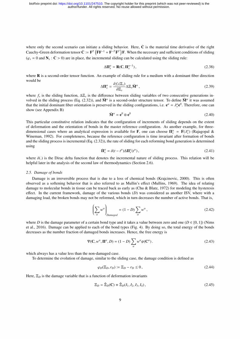
where fs is the sliding function, ∆Ξs is the difference between sliding variables of two consecutive generations in-volved in the sliding process (Eq. (2.32)), and Mα is a second-order structure tensor. To define Mα it was assumedthat the initial dominant fiber orientation is preserved in the sliding configurations, i.e. eα = λαs e0. Therefore, one canshow (see Appendix B)

Mα = e0 ⊗ e0 (2.40)

This particular constitutive relation indicates that the configuration of increments of sliding depends on the extentof deformation and the orientation of bonds in the master reference configuration. As another example, for three-dimensional cases where an analytical expression is available for F, one can choose Πα

s = F(λαs ) (Rajagopal &Wineman, 1992). For completeness, because the reference configuration is time invariant after formation of bondsand the sliding process is incremental (Eq. (2.32)), the rate of sliding for each reforming bond generation is determinedusing

Παs = δ(t − tα)∆Πα

s (tα) , (2.41)

where δ(.) is the Dirac delta function that denotes the incremental nature of sliding process. This relation will behelpful later in the analysis of the second law of thermodynamics (Section 2.6).

2.5. Damage of bonds

Damage is an irreversible process that is due to a loss of chemical bonds (Krajcinovic, 2000). This is oftenobserved as a softening behavior that is also referred to as Mullin’s effect (Mullins, 1969). The idea of relatingdamage to molecular bonds in tissue can be traced back as early as (Chu & Blatz, 1972) for modeling the hysteresiseffect. In the current framework, damage of the various bonds (D) was considered as another ISV, where with adamaging load, the broken bonds may not be reformed, which in turn decreases the number of active bonds. That is,∑

α

wα

Damaged

= (1 − D)∑α

wα , (2.42)

where D is the damage parameter of a certain bond type and it takes a value between zero and one (D ∈ [0, 1]) (Nimset al., 2016). Damage can be applied to each of the bond types (Fig. 4). By doing so, the total energy of the bondsdecreases as the number fraction of damaged bonds increases. Hence, the free energy is

Ψ(C,wα,Πα,D) = (1 − D)∑α

wαψ(Cα) . (2.43)

which always has a value less than the non-damaged case.To determine the evolution of damage, similar to the sliding case, the damage condition is defined as

ϕD(ΞD, rD) B ΞD − rD ≤ 0 , (2.44)

Here, ΞD is the damage variable that is a function of deformation invariants

ΞD = ΞD(C) ≡ ΞD(I1, I2, I3, I4) , (2.45)

9


https://doi.org/10.1101/247510

0 15 30 45 60 75

Time

0

0.5

1

Number-fraction

ofgen

erations(w

α)

w0w

1w

2

w3

w4

∑w

α = 1 −D

FormativeA

0 15 30 45 60 75

Time

0

0.5

1

PermanentB

0 15 30 45 60 75

Time

0

0.5

1

SlidingC

Figure 4. Effect of damage on kinetics: Multiple generations initiated at four consecutive step deformations at t = 0, 15, 30, 45with a first-order rate equation with damage shown for (A) formative bonds (B) permanent bonds and (C) sliding bonds, the sum ofbonds declines after each step of loading until the final value of 0.75 (D = 0.25). (For the references to color in this figure legend,the reader is referred to the web version of this article.)

and rD is the damage threshold defined as the maximum value of ΞD in the past history of deformation (Simo, 1987).The damage threshold rD is defined separately for each bond type as

rD B max

(r0)D, maxt∈(−∞,t]

ΞD(t). (2.46)

The value of rD before any loading is the initial damage threshold ((rD)0), which is a material property. Damageoccurs when ϕD = 0 (necessary condition). The loading direction determines the sufficient conditions. By definingthe second order tensorial normal to the damage surface (ϕD = 0) as

ND B∂ϕD

∂C|ϕD=0 , (2.47)

and by using the following normality conditions (Simo, 1987)ND : C ≤ 0 (no damage)

ND : C > 0 (damage); (2.48)

damage only occurs when (ϕD = 0 and ND : C > 0). Thus, during a damaging load, the damage parameter increasesaccording to the damage rule

D =∂ fD(ΞD)∂ΞD

ΞD , (2.49)

where fD(ΞD) is the damage function. Note that the damage variable (ΞD) is different from damage parameter (D),where D is the number fraction of permanently broken bonds.

2.6. Implications of the second law of thermodynamics

Any physical process must comply with the second law of thermodynamics, thus we check for compatibility ofreactive inelasticity with the second law of thermodynamics in terms of the Clausius-Duhem inequality. By ignoringthe thermal effects, the local form of Clausius-Duhem inequality reads as (Coleman & Gurtin, 1967)

D =12

S : C − Ψ(C,wα,Πα,D) ≥ 0 , (2.50)

whereD is the instantaneous local dissipation of energy, and for convenience will be referred to as dissipation. Here,(:) is the double contraction ((A : B)i j = Ai jBi j) and () stands for material time derivative (Holzapfel, 2000). Using

10


https://doi.org/10.1101/247510

the chain rule of differentiation and Eq. (2.11) we get12

S − (1 − D)∑α

wα ∂ψ(Cα)∂C

: C − (1 − D)∑α

wαψ(Cα)

−(1 − D)∑α

wα

(∂ψ(Cα)∂Πα

: Πα

)+D

∑α

wαψ(Cα) ≥ 0 .

(2.51)

Thus, to have a physically admissible process in the most general case each of the following conditions should beseparately satisfied (Coleman & Gurtin, 1967; Murakami, 2012)

S = (1 − D)∑α

wα2∂ψ(Cα)∂C

(2.52a)

D = DR +DD ≥ 0 , (2.52b)

where

DR = −(1 − D)∑α

(wαψ(Cα) + wα ∂ψ(Cα)

∂Πα: Πα

), and (2.53a)

DD = D∑α

wαψ(Cα) . (2.53b)

The first condition (Eq. (2.52a)) results in a new form of Eq. (2.12) where stress is scaled with damage. The secondcondition (Eq. (2.52b)) describes the dissipation of energy in a reactive inelastic process, where DR is dissipationdue to reactive bond breaking/reformations and change in reference configuration, and DD is the dissipation due todamage. The detailed proofs of the following results are included in Appendix C, and the following are the finalresults of reactive dissipation for each bond type.

We consider first only the dissipation due to bond breaking and reforming. For formative bonds, dissipation isalways positive because the breaking bonds (α < N) have a negative breakage rate, and the reforming bonds (α = N)are energy-free. That is,

(DR) f = −(1 − D f )N−1∑α=0

wαfψ(Cα) ≥ 0 . (2.54)

The permanent bonds dissipate no energy because there is no breakage and reformation occurring for these bonds:

(DR)p = 0 , (2.55)

and for sliding bonds dissipation is

(DR)s = −2δ(t − tN)(1 − Ds)∂ψ(CN

s )∂ΠN

s: ∆ΠN

s , (2.56)

where the Delta function form occurs due to the rate of sliding that was shown in Eq. (2.41). Half of this dissipationterm (Eq. (2.56)) is due to the process of breakage and reformation, and the other half is due to a shift in the referenceconfiguration. Accordingly, when the following condition is in place, the Clausius-Duhem inequality is satisfied

−∂ψ(CN

s )∂ΠN

s: ∆ΠN

s ≥ 0 . (2.57)

Equation (2.57) implies that at a given C, an increment of sliding only serves to reduce the energy level or equivalentlyto dissipate energy compared to a non-sliding case. Another implication of this condition is that once sliding hasdissipated all of the energy in the system, no further plastic deformation can occur and no further energy can be storedin the bonds.

11


https://doi.org/10.1101/247510

Considering the case where damage is involved D ≥ 0 and since the energy and number fraction of bonds havepositive values, the second term of Eq. (2.52b) is always positive. Therefore,

(DD)γ = D∑α

wαψ(Cα) ≥ 0 . (2.58)

Note that the above relation is only valid when there is no process of biological recovery and growth that may bepresent in living systems, where special considerations should be employed that are beyond the scope of this study.

In conclusion, as a consequence of the second law, formative and permanent bonds are ‘second-law compatible’ fora valid kinetics relation, and for sliding bonds, the change in reference configuration (Eq. (2.39)) needs to be definedso as to satisfy Eq. (2.57). For damage, fD (Eq. (2.49)) needs to be selected to guarantee D ≥ 0 (e.g., cumulativedistribution function of any continuous statistical distribution). Examples of appropriate constitutive relations will beprovided in Section 3.

2.7. Summary of formulationIn summary, a reactive inelasticity model was formulated that defines different types of bonds corresponding to

different mechanical behaviors. The combination of bond types should be selected according to the desired mechanicalbehaviors, where formative bonds should be used for a transient behavior with zero equilibrium stress, permanentbonds for a hyperelastic response, and sliding bonds should be used when a plastic deformation is occurring. Damagemay be added to each of the bond types, where it reduces the number fraction of active bonds, and thus reduces theability of material to absorb energy. In selecting the constitutive relations it is perhaps more convenient to take thediscrete steps that are outlined in Table 2.1. In the following section, several illustrative examples are provided thatboth help in understanding the model and also to exemplify some practical applications to mechanics of soft tissue,where reactive inelasticity can be useful.

3. Illustrative examples

To demonstrate key features of the reactive inelasticity framework we provide four numerical examples. First, thesensitivity of formative bonds to the kinetics rate is demonstrated using a Heaviside step loading that shows transitionsbetween different bond types (Example I). Second, we compare the stress response of the bond types to the classicalmodels; in particular the response of formative bonds is compared to quasi-linear viscoelasticity (QLV), permanentbonds to theoretical neo-Hookean hyperelastic material, and sliding bonds to a deformation-based plasticity model(Example II). Third, we simulate the stress response of an increasing cyclic loading by using a fiber-exponentialconstitutive relation that is commonly used in tissue mechanics, and we compare the stress response between non-damaged and damaged cases (Example III). Finally, incremental stress relaxation with softening is presented, whichhas importance to understand mechanisms of plasticity and damage in tissue. This is done by using a combination offormative bonds and either sliding bonds or permanent bonds with damage (Example IV). The model is implementedas a Matlab function using a custom written code intended for uniaxial deformations. The source code and details ofimplementation are provided as supplementary material and are accessible via the following online repository (Safa,2018).

For all of the examples, the axial component of the Cauchy’s stress tensor (i.e., T = T33) was used to represent thestate of stress during a uni-axial isochoric deformation

F = F(λ(t)) B ei ⊗ ei1√λ

+ e3 ⊗ e3(λ −1√λ

) i = 1, 2, 3 . (3.1)

The following constitutive relations were implemented in the steps outlined in Table 2.1:

• Step 1- Bond type selection: The bond type was selected depending on the expected mechanical behavior.Formative bonds were used for a viscoelastic behavior with zero equilibrium stress, permanent bonds for ahyperelastic behavior, and sliding bonds were used for plastic deformation. Note that for Example IV, whichincludes a combination of bonds, the response was calculated independently for each bond type and addedaccording to Eq. (2.11).

12


https://doi.org/10.1101/247510

Table 2.1. Summary of structure of a reactive bond type’s constitutive relations.Step 1 Select the bond types (i.e., formative, permanent, sliding)Step 2 Select the kinetics relation (e.g., Eq. (2.27))Step 3 Select the intrinsic hyperelasticity relation ψγ(Cα) (e.g., neo-Hookean)Step 4 If sliding bonds, select appropriate constitutive relations:

Sliding variable (Ξs) (Eq. (2.34))Sliding rule and function ( fs) (Eq. (2.39))

Step 5 If damage is included, select appropriate constitutive relations:Damage variable (ΞD) (Eq. (2.45))Damage rule and function ( fD) (Eq. (2.49))

• Step 2- Kinetics relation: For all of the examples, a first-order kinetics relation was used (Eq. (2.27)).

• Step 3- Intrinsic hyperelasticity: Three types of non-linear constitutive relations were used. First, we used theneo-Hookean relation in Examples I and II. This is the simplest non-linear constitutive relation and was used todemonstrate the general behaviors of the model, where the potential energy is

ψNH(I1) = C1(I1 − 3) . (3.2)

Here, C1 is the independent model parameter with dimensions of stress.

Second, for relevance to tissue applications, in Examples III and IV we used a one-dimensional exponentialconstitutive relation with a non-zero stiffness only in the e3 direction (fiber direction) in tension (Jacobs et al.,2014; Schmidt et al., 2014)

ψEF(I4) = C2

(exp

[C3(I4 − 1)2

]− 1

)u(I4 − 1) , (3.3)

where C2 and C3 are positive-valued model parameters.

Third, for showing a three-dimensional tissue mechanics application, we used a Holmes-Mow material (Exam-ple IV)

ψHM(I1, I2, I3) = α0

(I−β3 exp [α1(I1 − 3) + α2(I2 − 3)] − 1

). (3.4)

In this relation, α0 is a positive number with the dimension of stress and [β, α1, α2] are positive non-dimensionalnumbers. To comply with the energy- and stress-free reference configuration, β = α1 + 2α2 must be satisfied(Holmes & Mow, 1990). It also should be noted that the Holmes-Mow model parameters are related to the morefamiliar infinitesimal linear-elastic parameters as:

α1 =E/α0

4(1 + ν)− α2 , and α2 =

(E/α0)ν4(1 + ν)(1 − 2ν)

, (3.5)

where E is the Young’s modulus, and ν is the Poisson’s ratio. Hence, [E, ν] were used in the following insteadof the original Holmes-Mow parameters.

• Step 4- Sliding: The overall stretch was selected as the sliding variable

Ξs = λ =√

I4 . (3.6)

To describe the sliding rule for the one-dimensional fiber intrinsic hyperelasticity relation (Example II) (Eq. (3.3))the form represented in Eq. (2.39) was employed with the sliding function as

fs(Ξs) = c (Ξs − (rs)0)b , (3.7)

where the constant parameters [c, b] are dimensionless positive numbers, and (r0)s is the initial sliding threshold.Also, e3 was taken as the sliding direction and was used to define structural direction tensor as M B e3 ⊗ e3(Eq. (2.39)). In this case, as long as λN−1

s < λNs < λ the condition of Eq. (2.57) is satisfied, and it can be

13


https://doi.org/10.1101/247510

easily verified that(−∂ψEF(λ/λN

s )/∂λNs

) (λN

s − λN−1s

)> 0, which proves the compatibility of these constitutive

relations with the second law. For the three-dimensional constitutive relation cases (Examples I,II,IV) it wasassumed that ΠN

s takes the form of F(λNs ) during sliding, where by using the Taylor series expansion, it can be

shown that all of the constitutive equations are compatible with the second law of thermodynamics (for detailssee Appendix C).

• Step 5- Damage: For the case with damage of bonds, similar to sliding, the overall stretch was used as thedamage variable

ΞD =√

I4 , (3.8)

and a Weibull’s cumulative distribution function was used as the damage function (Nims et al., 2016)

fD(ΞD) = 1 − exp

− (ΞD − (rD)0

l − 1

)k , (3.9)

where k is the shape parameter, l is the scale parameter, and (r0)D is the initial damage threshold.

3.1. Sensitivity of the formative bonds to the kinetics rate (Example I)

As discussed in Section 2, the kinetics rate is the predominant difference between various bond types. To show this,we simulated the response of formative bonds to a Heaviside step deformation at a wide range of reaction kinetics rate,where the only variable was the time constant (τ f ) (Fig. 5). For a large τ f (slow kinetics rate) the response approachesthe hyperelastic behavior (permanent bonds), and as τ f gets smaller (high kinetics rate) the response approaches asingular stress behavior (sliding bonds). For all of the kinetics rates, the response at t = 0 is the same and equal tothe hyperelastic stress for that deformation. This response at t = 0 also corresponds to the peak stress response of theinitial generation in Eqs. (2.24) and (2.25).

This simple example lies at the heart of reactive inelasticity and demonstrates the consistency of inelastic behaviorsthat are all based on the kinetics of breaking and reforming bonds. In what follows, more complex loading scenariosare investigated that are all based on a summation of incremental step deformations.

3.2. Response of various bond types and comparison to classic models (Example II)

Example II is the stress response of the three bond types to a simple loading/un-loading deformation (Fig. 6A)with a neo-Hookean constitutive relation for intrinsic hyperelasticity. Formative bonds show stress relaxation, whichis a common characteristic of a viscoelastic response (Fig. 6B, E). Permanent bonds show a one-to-one relation be-tween deformation and stress with no history dependence (hyperelastic) (Fig. 6C, F). Sliding bonds show a differencebetween loading and unloading, where during loading, the state of zero-stress was shifted, which indicates a plasticdeformation (Fig. 6D, G) .

We compared the response of the three bond types to classic models (model parameters are detailed in Table D.1).In particular, the response of formative bonds is compared to quasi-linear viscoelasticity (QLV) (Fig. 6B,E) (Fung,1993), where

TQLV (λ(t)) =

∫ t

−∞

exp(u − tτ

)TNH(λ(u))du , (3.10)

and TNH is determined using Eqs. (2.20) and (3.4). The response of permanent bonds is compared to the theoreticalhyperelastic response of a neo-Hookean material (Fig. 6C, F). Lastly, the response of sliding bonds is compared to asimple deformation-driven plasticity model (Fig. 6D, G), where

TPLAS T IC(λ, λp) = TNH(λ/λp) . (3.11)

Here λ corresponds to stretch, also note that the superscript p indicates the plastic part of deformation. For post-yieldloading λp is calculated as

λp = 1 + c(Ξ − (r0)Y )b , (3.12)

where Ξ = Ξs and (r0)Y = (r0)s, also [c, b] have the same values as in the sliding constitutive relations.

14


https://doi.org/10.1101/247510

0 20 40 60 80 100

Time

0

20

40

60Axialstress

(T)

Increaseτf

Permanent (τf → ∞)

Formative

Sliding (τf → 0)

(τf )0 × 25

(τf )0 × 23

(τf )0 × 22

(τf )0 × 21

(τf )0(τf )0 × 2−1

(τf )0 × 2−2

(τf )0 × 2−3

(τf )0 × 2−5

Figure 5. Example I: Time response of formative bonds to a Heaviside-step deformation in a large range of kinetics. Thekinetics rate is controlled by time constant of reaction where (τ f )0 = 10 and the range of time constants is covered by multiplying(τ f )0 with powers of two. Formative bonds show an asymptotic decay in Cauchy stress during a sustained loading, whereas forlarge values of τ f (slow kinetics rate) the response approaches a hyperelastic behavior (permanent bonds) marked with dashed redline, and at small τ f (high kinetics rate), the stress response approaches a singular behavior that is immediately decays to zero(sliding bonds). The step deformation is λ(t) = 1.1u(t) and the neo-Hookean intrinsic hyperelasticity parameter is C1 = 100. (Forreferences to color in this figure legend, the reader is referred to the web version of this article.)

Reactive inelasticity successfully reproduced each of the classical models. Note that for large deformations, theconclusions are valid for permanent bonds; however, the behavior of formative bonds and QLV slightly deviate,which is due to the Boltzmann’s superposition principle in QLV (Ateshian, 2015). For plastic deformation, althoughthere is no difference between the stress response of deformation-based plasticity model and reactive sliding, thetwo approaches indicate different physical meanings, where by simply shifting the reference configuration (as inthe deformation-based formulation) the process of breakage and reformation is not considered. Mechanistically, aninelastic bond sliding should occur as an explicit consequence of a bond dissociation and reattachment, and thus wesuggest that the reactive interpretation of this process is physically appropriate. From these examples, it is evidentthat the reactive inelasticity framework is capable of reproducing various mechanical behaviors, where the same setsof constitutive relations are used for each of the bond types.

3.3. Cyclic loading and damage (Example III)

Example III demonstrates the response of single bond types with the model parameters listed in Table D.2 to acyclic loading (Fig. 7A). In response, formative bonds dissipate energy in a cyclic hysteresis (Fig. 7B), while thepermanent bonds have a hyperelastic response that is independent of history of deformation (Fig. 7C). The slidingbonds undergo plastic deformation that is evident by the shift in the point of zero stress after each cycle, while thereis no change in stiffness during the consecutive loading parts (Fig. 7D). Note that the sliding bonds account for strainsoftening that results in a decrease in stress after reaching the peak stress (points 3 and 4 in Fig. 7D), and it is differentfrom strain hardening that is associated with plasticity in metals and some engineering polymers. Further, by addingdamage (decreasing the total number of bonds) the Mullin’s effect was captured for all three types of bonds. Inaddition to decreasing stiffness and the corresponding stress values, the damage increases the difference between theloading and unloading parts of the stress response. This results in increased hysteresis and further dissipation ofenergy (Fig. 7E, F, and G).

The expansion of sliding and damage thresholds are shown in Fig. 7A by the dashed lines. It is evident fromthe simulations that the behavior of bonds, especially permanent bonds with damage and sliding bonds are similar.However, certain characteristics are unique to each bond type. For example, contrary to sliding bonds, there is noshift in reference configuration for permanent bonds with damage. Importantly, from an experimental perspective, itis not possible to distinguish the mechanical response of plastic deformation from that of damage in loading, and theirdifference becomes evident only in unloading.

15


https://doi.org/10.1101/247510

0 25 50 75 100

Time

0.95

1

1.05

1.1

1.15

1.2

Stretch

(λ)

A

Stretch (λ)

rs

0 25 50 75 100

Time

-40

-20

0

20

40

Axialstress

(T)

B

Formative bonds

QLV

0 25 50 75 100

Time

-20

0

20

40

60

80

Axialstress

(T)

C

Permanent bonds

Neo-Hookean

0 25 50 75 100

Time

-20

0

20

40

60

Axialstress

(T)

D

Sliding bonds

Plastic Def.

1 1.05 1.1

Stretch (λ)

-40

-20

0

20

40

Axialstress

(T)

E

Formative bonds

QLV

1 1.05 1.1

Stretch (λ)

-20

0

20

40

60

80

Axialstress

(T)

F

Permanent bonds

Neo-Hookean

1 1.05 1.1

Stretch (λ)

-20

0

20

40

60Axialstress

(T)

G

Sliding bonds

Plastic Def.

Figure 6. Example II: Mechanical response of different bond types to a simple loading/un-loading deformation. (A) Stretchprofile of loading, and evolution of the sliding threshold. In (B,E) formative bonds were compared to quasi-linear viscoelasticity,(C,F) compares permanent bonds to the theoretical stress response of a neo-Hookean material, and (D,G) shows the comparisonbetween sliding bonds’ response and a plasticity model in deformation space.

3.4. Incremental stress relaxation with softening (Example IV)

In Example IV a typical response of tissue in a stress relaxation test is demonstrated that also includes softening.Softening in tissues often occurs at high deformations (Szczesny & Elliott, 2014; Lynch et al., 2003). It is not possibleto distinguish between damage and plastic deformation solely by loading the tissue in tension and analyzing the stressresponse. This is demonstrated in the example by using a combination of formative bonds and either sliding bonds, orpermanent bonds with damage (Fig. 8). In these examples, formative bonds account for the transient stress response,and sliding (or permanent bonds) produce the equilibrium part of the stress response (model parameters in Table D.3).Identical behaviors are observed during ramp and relaxation loading phases (Fig. 8). However, during unloading it isevident that the reference configuration is shifted when implementing the sliding bonds, where for permanent bondswith damage there is no shift in the zero-stress configuration.

Experimental evaluation of this shift in the reference configuration in soft tissue is often challenging due to non-linearity in stress-strain behavior, when the initial stiffness is low that gradually increases by further deformation(toe-region effect). However, by having a theoretical framework for both of the candidate mechanical behaviors (i.e.,plastic deformation and damage) it is possible to fit the models to the loading phase and make predictions about either

16


https://doi.org/10.1101/247510

0 20 40 60 80

Time

1

1.02

1.04

1.06

1.08

1.1

Stretch

(λ)

1

2

3

4

A

Stretch (λ)

rs

rD

1 1.05 1.1

Stretch (λ)

0

1

2

3

Axialstress

(T)

1

2

3

4

FormativeB

Non-d

am

aged

1 1.05 1.1

Stretch (λ)

0

1

2

3

Axialstress

(T)

1

2 34

E

Dam

aged

1 1.05 1.1

Stretch (λ)

0

2

4

6

8

10

Axialstress

(T)

12

3

4PermanentC

1 1.05 1.1

Stretch (λ)

0

1

2

3

4

5

Axialstress

(T)

1

2

3

4

F

1 1.05 1.1

Stretch (λ)

0

0.5

1

1.5

2

Axialstress

(T)

1

2

34

SlidingD

1 1.05 1.1

Stretch (λ)

0

0.5

1

1.5

2

Axialstress

(T)

1

2

3

4

G

Figure 7. Example III: Cyclic loading and damage (A) an increasing cyclic loading protocol applied for non-damaged (B)formative, (C) permanent, (D) sliding bonds. When damage is added to the response for (E) formative, (F) permanent, and (G)sliding bonds, all the bond types show a softening behavior. The evolution of sliding and damage thresholds is also shown in (A)in response to loading and unloading phases, where sliding starts after λ = (rs)0 = 1.01, and damage after λ = (rD)0 = 1.03.

the unloading phase, or other experimental results (e.g., cyclic loading in Example III) to assess the success of themodel in predicting the experimental data, and thus evaluating the contribution of each of the aforementioned inelasticbehaviors in tissue.

4. Discussion and concluding remarks

This study provides a structurally inspired framework for modeling inelasticity in tissue. It uses a thermodynamicscheme, where internal state variables and kinetics of molecular bonds are employed to capture the major inelasticbehaviors of tissue. This framework consistently addresses a range of inelastic behaviors. The formative, permanent,and sliding bonds correspond to viscoelastic behavior with zero equilibrium stress, hyperelastic response, and plastic

17


https://doi.org/10.1101/247510

0 20 40 60 80 100

Time

0

1

2

3

4

5

6Axialstress

(T)

A

Total

Sliding

Formative

1 1.02 1.04 1.06 1.08

Stretch (λ)

0

1

2

3

4

5

6

Axialstress

(T)

C

Total

Sliding

Formative

0 20 40 60 80 100

Time

0

1

2

3

4

5

6

Axialstress

(T)

B

Total

Perm. + Dam.

Formative

1 1.02 1.04 1.06 1.08

Stretch (λ)

0

1

2

3

4

5

6

Axialstress

(T)

D

Total

Perm. + Dam.

Formative

Figure 8. Example IV: Incremental stress relaxation with softening for (A,C) formative and sliding bonds, and (B,D) formativebonds with permanent bonds and damage. The effect of selection of either sliding bonds or permanent bonds is only observed duringunloading. When the sliding bonds are used there is a shift in the reference configuration (C) which is not true for permanent bondswith damage (D).

deformation, respectively. Additionally, the formulation of bond kinetics allows for the inclusion of damage byreducing the number of bonds, which introduces damage as an inelastic behavior to all of the bond types. Anycombination of the bond types can be employed to model various kinds of inelastic behaviors, such as a combinationof formative bonds and permanent bonds with damage to model a viscoelastic behavior with softening.

The reactive inelasticity framework is structurally inspired, thus the concept of bonds and their energy level havephysical relevance—unlike the majority of the phenomenological models. Connective tissue’s matrix is mostly madeof cross-linked collagen. These molecules are cross-linked to each other via several mechanisms including enzymaticlysyl oxidase-mediated and non-enzymatic glycation-induced cross-links to produce larger collagenous structures(Reiser et al., 1992; Eyre et al., 2008). The mechanical properties of collagenous material are sensitive to the den-sity, structure and properties of these cross-links (Depalle et al., 2015). When overloaded, collagen fibrils show localdeformities (e.g., kinks) that contain denatured-collagen-rich regions (Herod et al., 2016; Veres et al., 2014). Recentadvancements in using collagen hybridizing peptides (CHP) provides opportunities to visualize the spatial distribu-tion and level of disruption in these regions after mechanical overloading (Li & Yu, 2013; Zitnay et al., 2017). Theseobservations suggest that there is a strong correlation between mechanical loading and the state of molecular bonding.Two potential mechanisms of molecular disruption, shear and tension dominant, were suggested based on molec-ular dynamics experiments that closely resemble the sliding and damage processes (Zitnay et al., 2017). Despitethese advancements in visualizing the molecular state of tissue and its relation to their mechanical behavior, furtherexperimental work needs to be done to elucidate structural mechanisms of inelasticity in terms of molecular bonding.

The reactive inelasticity framework is a generalization of the reactive viscoelasticity model (Ateshian, 2015),where an inclusive and consistent treatment of inelastic processes is provided. The reactive viscoelasticity modelof Ateshian provided the essential concepts of weak and strong bonds that correspond to formative and permanentbonds, respectively. We chose the terminology of formative and permanent bonds because of their analogy to kinetics

18


https://doi.org/10.1101/247510

rate of bonds and their behavior. Additionally, in contrast to (Ateshian, 2015) we based our formulation on thenumber fraction of bonds rather than mass fraction, which emphasizes that in general, bonds are levels of energyand individual bonds do not correspond to a physical mass. Although at the first sight these parameters appear tobe equivalent, due to their non-dimensional nature, this non-inertial bond assumption is particularly important whenconsidering the singular accelerations arising in the case of sliding bonds. Massless bonds keep the model in therealm of admissibility in the general sense. Further, by making these generalizations we showed that the bonds areinterchangeable at the extremes of kinetics rate, where the behavior of formative bonds is hyperelastic (permanentbonds) in the limit of slow kinetics rate (Fig. 5), and at high rates of bond kinetics formative bonds turn into slidingbonds that correspond to a plastic deformation (Figs. 6 and 7).

Plastic deformation has been experimentally observed in tissue at the macro- (Maher et al., 2012), micro- (Szczesny& Elliott, 2014; Lee et al., 2017), and nano-scale (Shen et al., 2008). Several phenomenological ISV modeling ap-proaches have been taken to address these phenomena that often are focused to address specific inelastic behaviorsand usually omit the relationships between different inelastic behaviors and their mechanisms (Zhang & Sacks, 2017;Fereidoonnezhad et al., 2016; Pena, 2014; Maher et al., 2012). In the current framework, we particularly focused onproviding a consistent formulation between different inelastic behaviors and their structural relevance. In a similarmanner, for cross-linked polymers a molecular bond approach has been used to model stress relaxation and plasticnecking instability (Meng & Terentjev, 2016; Meng et al., 2016); however, in that theory, only plastic necking ratherthan general plastic deformation was addressed, and therefore, their formulation does not explicitly provide for theshift in unloaded configuration that is observed in tissue, such as non-recoverable interfibrillar sliding (Lee et al.,2017). In our model, the generation reference deformation gradient (Πα) is a state variable that is directly related tothe plastic deformation and thus is an observable variable accounting for the shift in unloaded configuration of thematerial.

Damage was applied to each of the bond types regardless of their kinetics rate. This allowed for modeling theeffect of damage on different components of structure that produce the mechanical behavior of material, such asdegradation in the viscous components of a viscoelastic behavior without affecting its elastic part. Previously, asimilar concept was used to study damage in cartilage that was only applied to the permanent bonds. This resulted inthe damage effect being limited to the equilibrium behavior (Nims et al., 2016). The reduction in number fraction ofactive bonds results in a decrease in the ability of material to absorb energy, which provides a generalized definitionof damage as a behavior. By adding this ability, it is possible to model mechanical behavior up to rupture, where,if the formative bonds could not be damaged, no rupture could occur. Another benefit of this definition is in that itforms a clear theoretical basis for distinction between plastic deformation and damage. As shown in Fig. 7, plasticdeformation alone does not result in a decrease in stiffness; however, adding damage would cause a reduction instiffness, which is a common mechanical property used to assess the extent of damage in a material. By using thecurrent theoretical framework for addressing damage and other forms of inelastic response that was provided in thisstudy, it is possible to elucidate the mechanisms and role of each inelastic behavior in the mechanical response of tissuefrom the experimental stress response of the material. One future direction, for example, is using a specific loadingprofile with repeated scenarios (e.g., loading, unloading and reloading) to curve fit different versions of reactiveinelasticity and using the fit parameters to predict an independent experimental mechanical behavior. From the qualityof the predictions, one can assess the relevance of the involved inelastic behaviors and their contribution.

In this framework, one of the limitations may be that we made a continuum body assumption to relate the molecularenergy to the macro-scale mechanical behavior, where hierarchical structural effects, as well as statistical consider-ations for molecular bonding were not included; however, the simplicity of the model and its ability to reproduce aspectrum of macro-scale behaviors were chosen here over complexity of formulation. Additionally, we modeled theplastic deformation by using a finite-strain framework with a constrained direction, and damage was modeled as ascalar variable that may overly constrain a generalized three-dimensional case (Ju, 1990). These issues can be ad-dressed by adding multiple bond types with different directional preferences to achieve a desired spatial characteristic(Nims et al., 2016). Finally, since tissues have a significant fluid content, the fluid pressurization and flow can play animportant role in the mechanical response. Those effects were not included in this model, which is a limiting factor forapplying this framework to experimental data. However, the effect of fluid content can be added as in a multiphasicmixture model with inelastic solid phase that uses reactive inelasticity (Huang et al., 2001).

In conclusion, we have provided a structurally inspired framework for modeling inelastic behaviors of tissue basedon the kinetics of reactive molecular bonds that break and reform in response to mechanical loading. The model ad-

19


https://doi.org/10.1101/247510

dresses viscoelasticity, plastic deformation, and damage in an inclusive framework. We introduced three types ofmolecular bonds: formative, permanent, and sliding that result in viscoelastic, hyperelastic, and plastic deformationbehaviors. Damage was applied to each of the bond types by reducing the number fraction of bonds, which conse-quently decreases the ability of material to absorb energy. All of the aforementioned inelastic behaviors are modeledwithin the same framework and by using similar sets of constitutive equations. This allows for investigating themechanisms of inelasticity by providing a comprehensive theoretical basis for analyzing the mechanical response oftissue that can be used to understand mechanical loading induced pathological conditions, to develop more effectivetreatment protocols, and to engineer replacement tissues.

5. Conflict of interest

Authors have no conflicts of interest to disclose.

6. Acknowledgment

Research reported in this publication was supported by the National Institute of Biomedical Imaging and Bioengi-neering of the National Institutes of Health under award number R01EB002425. The content is solely the responsi-bility of the authors and does not necessarily represent the official views of the National Institutes of Health.

Appendix A. Stress and relative deformation

By using the definition of free energy of the system from Eq. (2.11) the second Piola-Kirchhoff stress tensorfor a bond type in terms of number fraction of bonds (wα) and relative deformation (represented by relative rightCauchy-Green deformation Cα) is

S = 2∂Ψ(Cα)∂C

=∑α

2wα ∂ψ(Cα)∂C

. (A.1)

Using the chain rule of differentiation and Einstein’s index notation:

∂ψ

∂Ci j=

∂ψ

∂Cαmn

∂Cαmn

∂Ci j. (A.2)

Using Eq. (2.2) and noting that the reference deformation gradient tensor (Πα) is fixed for a specific generation;

∂Cαmn

∂Ci j=∂((Πα

pm)−1Cpq(Παqn)−1)

∂Ci j

= (Παpm)−1δpiδq j(Πα

qn)−1

= (Παim)−1(Πα

jn)−1 .

(A.3)

By substituting this result in Eq. (A.2) we get

∂ψ

∂Ci j=

∂ψ

∂Cαmn

(Παim)−1(Πα

jn)−1 . (A.4)

Or, in tensor notation∂ψ(Cα)∂C

= (Πα)−1ψ(Cα)∂Cα

(Πα)−T . (A.5)

Substituting this result back in Eq. (A.1) gives

S =∑α

2wα(Πα)−1ψ(Cα)∂Cα

(Πα)−T , (A.6)

which provides the full form of the second Piola-Kirchhoff stress for a bond type in a reactive material, Eq. (2.13).

20


https://doi.org/10.1101/247510

Appendix B. Proof of the structure tensor (Mα) expression in Eq. (2.40)

By assuming that the stretch in the fiber direction for the reference configuration of the α generation is λαs ,which has a value that is infinitesimally different from that of generation (α− 1), and by using Taylor’s approximationone can show

(λαs )2 ≈ (λα−1s )2 + 2(λα−1

s )∆λαs . (B.1)

Additionally, based on Eq. (2.32) from the corresponding sliding configuration deformation gradients we have:

(λαs )2 = e0s(Πα

s )T Παs e0

s

= e0s

[((Πα−1

s )T + (∆Παs )T

) (Πα−1

s + ∆Παs

)]e0

s

≈ e0s

[(Πα−1

s )T Πα−1s + (∆Πα

s )T Πα−1s + (Πα−1

s )T ∆Παs

]e0

s

. (B.2)

By combining Eqs. (B.1) and (B.2) and by substituting (λα−1s )2 = e0

s(Πα−1s )T Πα−1

s e0s we get

e0s

[(∆Πα

s )T Πα−1s + (Πα−1

s )T ∆Παs

]e0

s = 2(λα−1s )∆λαs . (B.3)

Therefore, by assuming eα−1s = e0

s , one can easily show that

∆Παs = ∆λαs e0

s ⊗ e0s (B.4)

holds. Finally, by taking that ∆λαs = ∂Ξs fs(Ξs)∆Ξs the expression Mα = e0s ⊗ e0

s is resulted in terms of Eq. (2.39). Thisrelation indicates that during sliding, the dominant fiber direction is preserved and only the reference length changes.This relation can be enhanced by including the effect of permanent changes to the dominant fiber direction as seenin some fibrous tissues, such as the intervertebral disc (Dittmar et al., 2016), by using phenomenological relations tocorrelate e0

s and eα−1s .

Appendix C. Reactive dissipation due to reactive bond breaking and reformation

In the following, we investigate the compatibility of different bond types with the second law of thermodynamics.At a given time, consider a set of bonds from the same type that are grouped into breaking generations (α ∈ 0, . . . , (N−1)) and a reforming generation (α = N), hence Eq. (2.53a) can be rearranged into

DR = −(1 − D)

N−1∑α=0

wαψ(Cα) + wα ∂ψ(Cα)∂Πα

: Πα

︸︷︷︸breaking generations

+

(wNψ(CN) + wN ∂ψ(CN)

∂ΠN : ΠN)

︸︷︷︸reforming generation

. (C.1)

Appendix C.1. Formative bondsAccording to Eq. (2.27) for all of the breaking bonds we have

wαf < 0 , (C.2)

and we know in general that the free energy in a deformed state is considered positive

ψ f (Cα) > 0 . (C.3)

Additionally, the reforming bonds reform in an energy free state (Section 2.4.1)

ψ f (CN = I) = 0 . (C.4)

For the breaking formative bonds the reference deformation gradient is fixed (Παf = 0, α < N) and for their reforming

generation (α = N) (Eq. (2.30))

ΠNf = ΠN−1

f + u(t − tN)∆ΠNf , and ΠN

f = δ(t − tN)∆ΠNf , (C.5)

21


https://doi.org/10.1101/247510

where u(t) denotes the unit step function, and δ(t) is the Dirac delta function. Further, using Eq. (2.28) one can show

wNf ΠN

f = δ(t − tN)wNf ∆ΠN

f = 0 . (C.6)

Therefore, for formative bonds

(DR) f = −(1 − D f )N−1∑α=0

wαfψ(Cα) ≥ 0 , (C.7)

which indicates that during breaking and reformation of formative bonds, dissipation is positive and is due solely tobreakage of bonds.

Appendix C.2. Permanent bondsSince for these bonds there is just one generation and there is no breakage and reformation, we have (w0

p = 0 andΠ0

p = I) as a result(DR)p = 0 . (C.8)

This result denotes that there is no dissipation of energy for permanent bonds due to a lack of reactive breaking andreformation.

Appendix C.3. Sliding bondsFor these bonds, the only generations with non-zero dissipation terms are the last breaking (α = N − 1) and the

reforming generations (α = N). Their number fractions and kinetics rates are (Section 2.4.3)

wN−1s (t) = 1 − u(t − tN) , wN

s (t) = u(t − tN) , (C.9a)

wN−1s (t) = −δ(t − tN) , wN

s (t) = δ(t − tN) . (C.9b)

In addition, according to Eqs. (2.32) and (2.41) the corresponding Πs for those bonds during sliding reads as

ΠN−1s (t) = 0 , and ΠN

s (t) = δ(t − tN)∆ΠNs . (C.10)

As a result

(DR)s = δ(t − tN)(1 − Ds)[(ψ(CN−1

s ) − ψ(CNs )

)−∂ψ(CN

s )∂ΠN

s: ∆ΠN

s

]= −2δ(t − tN)(1 − Ds)

∂ψ(CNs )

∂ΠNs

: ∆ΠNs ,

(C.11)

where we used the Taylor series to write ψ(CNs )−ψ(CN−1

s ) ≈ (∂ψ(CNs )/∂ΠN

s ) : ∆ΠNs . Therefore, half of this dissipation

is driven by the process of breakage and reformation, and the other half is explicitly due to a shift in the referenceconfiguration. The above relation corresponds to a positive value for dissipation when

−∂ψ(CN

s )∂ΠN : ∆ΠN ≥ 0 . (C.12)

For the constitutive relations and deformation used in this paper, we can analytically verify the above inequality asfollows.

Appendix C.3.1. Exponential fibersSince the only non-zero component of the deformation and stress is in the fiber direction, a one dimensional

formulation can be used for convenience, where ΠNs is represented by λN

s . As a result, the inequality (C.12) reads as

−∂ψEF(IN

4 )∂ΠN : ∆ΠN = −

∂ψEF(λ/λNs )

∂λNs

∆λNs

= 4C2C3

(λ

λNs

)3

exp

C3

( λλN

s

)2

− 1

2( λλN

s

)2

− 1

∆λNs

λ

(C.13)

where ∆λNs = λN

s − λN−1s . As a result, since λN−1 < λN < λ the above expression has a positive value.

22


https://doi.org/10.1101/247510

Appendix C.3.2. Neo-HookeanBecause of the assumption that F = F(λ), ∆ΠN can be written as F(λN

s ) − F(λN−1s ) and by using the Taylor’s

expansion

∆ΠN =

− 1

2 (λN−1s )−

32 0 0

0 − 12 (λN−1

s )−32 0

0 0 1

∆λNs , (C.14)

also, one can write

∂ψNH(IN1 )

∂ΠN = −2C1

(λN

s )32

λ0 0

0 (λNs )

32

λ0

0 0 λ2

(λNs )3

. (C.15)

Therefore, the inequality (C.12) up to the first order relative to ∆λNs , reads as

−∂ψNH(Iα1 )∂ΠN : ∆ΠN ≈ 2C1

( λλN

s

)3

− 1

∆λNs

λ≥ 0 , (C.16)

which is clearly valid when λN−1 < λN < λ.

Appendix C.3.3. Holmes-MowThe ∆ΠN is the same as in the Neo-Hookean case (Eq. (C.14)), and similarly the inequality is calculated as

−∂ψHM(Iα1 , I

α2 , I

α3 )

∂ΠN : ∆ΠN ≈ 2α0 exp (A)(α1 + α2

λNs

λ

) ( λλN

s

)3

− 1

∆λNs

λ≥ 0 , (C.17)

whereA = α1(Iα1 − 3) + α2(Iα2 − 3) . (C.18)

That also indicates since λN−1 < λN < λ the conditions of the second law are met for sliding.

Appendix D. Model parameters used in the illustrative examples

The illustrative examples were designed using the noted constitutive relations to demonstrate the important fea-tures of the framework with no particular focus on certain tissues; however, in practice, specific constitutive relationsshould be employed to use the framework for successfully modeling of the inelastic behaviors of tissue. The modelsgenerated with this framework may have different number of model parameters. Thus, in general, no specific numberof parameters could be associated with the framework. Below we have listed the model parameters used for differentexamples.

Table D.1. Parameters used for comparison of reactive inelasticity to classic models (Fig. 6).τ C1 c b (r0)s

Formative 10 100 - - -Permanent 1010 100 - - -Sliding 0.01 100 10 2 1.05

Table D.2. Parameters used for dynamic response of single bond types (Fig. 7).τ C2 C3 c b (r0)s k l (r0)D

Formative 10 0.1 40 - - - - - -Permanent 1010 0.1 40 - - - 2 1.04 1.03Sliding 0.01 0.1 40 9 2 1.01 - - -

23


https://doi.org/10.1101/247510

Table D.3. Parameters used for the incremental stress relaxation response tests (Fig. 8).τ C2 C3 E v α0 c b (r0)s k l (r0)D

Formative 10 0.1 40 - - - - - - - - -Permanent 1010 - - 50 0.3 0.1 - - - 2 1.05 1.02Sliding 0.01 - - 50 0.3 0.1 8 2 1.02 - - -

References

Alastrue, V., Rodrıguez, J., Calvo, B., & Doblare, M. (2007). Structural damage models for fibrous biological soft tissues. International Journalof Solids and Structures, 44, 5894–5911. URL: http://www.sciencedirect.com/science/article/pii/S0020768307000741http://linkinghub.elsevier.com/retrieve/pii/S0020768307000741. doi:10.1016/j.ijsolstr.2007.02.004.

Andrews, R. D., Tobolsky, A. V., & Hanson, E. E. (1946). The Theory of Permanent Set at Elevated Temperatures in Natural and Synthetic RubberVulcanizates. Journal of Applied Physics, 17, 352–361. URL: http://aip.scitation.org/doi/10.1063/1.1707724. doi:10.1063/1.1707724.

Ateshian, G. A. (2015). Viscoelasticity using reactive constrained solid mixtures. Journal of Biomechanics, 48, 941–947. URL: http://www.sciencedirect.com/science/article/pii/S0021929015000986http://linkinghub.elsevier.com/

retrieve/pii/S0021929015000986. doi:10.1016/j.jbiomech.2015.02.019.Caro-Bretelle, A., Gountsop, P., Ienny, P., Leger, R., Corn, S., Bazin, I., & Bretelle, F. (2015). Effect of sample preservation on stress softening and

permanent set of porcine skin. Journal of Biomechanics, 48, 3135–3141. doi:10.1016/j.jbiomech.2015.07.014.Chu, B. M., & Blatz, P. J. (1972). Cumulative microdamage model to describe the hysteresis of living tissue. Annals of Biomedical Engineering,

1, 204–211. URL: http://link.springer.com/10.1007/BF02584207. doi:10.1007/BF02584207.Coleman, B. D., & Gurtin, M. E. (1967). Thermodynamics with Internal State Variables. The Journal of Chemical Physics, 47, 597–613. URL:

http://scitation.aip.org/content/aip/journal/jcp/47/2/10.1063/1.1711937. doi:10.1063/1.1711937.Connizzo, B. K., & Grodzinsky, A. J. (2017). Tendon exhibits complex poroelastic behavior at the nanoscale as revealed by high-frequency AFM-

based rheology. Journal of Biomechanics, 54, 11–18. URL: http://linkinghub.elsevier.com/retrieve/pii/S0021929017300428.doi:10.1016/j.jbiomech.2017.01.029.

Cortes, D. H., & Elliott, D. M. (2014). Accurate prediction of stress in fibers with distributed orientations using generalized high-order structuretensors. Mechanics of Materials, 75, 73–83. URL: http://linkinghub.elsevier.com/retrieve/pii/S0167663614000714. doi:10.1016/j.mechmat.2014.04.006.

Demirkoparan, H., Pence, T. J., & Wineman, A. (2009). On dissolution and reassembly of filamentary reinforcing networks in hypere-lastic materials. Proceedings of the Royal Society A: Mathematical, Physical and Engineering Sciences, 465, 867–894. URL: http:

//rspa.royalsocietypublishing.org/cgi/doi/10.1098/rspa.2008.0360. doi:10.1098/rspa.2008.0360.Depalle, B., Qin, Z., Shefelbine, S. J., & Buehler, M. J. (2015). Influence of cross-link structure, density and mechanical properties in the mesoscale

deformation mechanisms of collagen fibrils. Journal of the Mechanical Behavior of Biomedical Materials, 52, 1–13. doi:10.1016/j.jmbbm.2014.07.008.

Diani, J., Fayolle, B., & Gilormini, P. (2009). A review on the Mullins effect. URL: https://www-sciencedirect-com.udel.idm.oclc.org/science/article/pii/S0014305708006332. doi:10.1016/j.eurpolymj.2008.11.017.

Dittmar, R., Van Rijsbergen, M. M., & Ito, K. (2016). Moderately Degenerated Human Intervertebral Disks Exhibit a Less Geometrically SpecificCollagen Fiber Orientation Distribution. Global Spine Journal, 6, 439–446. URL: http://www.ncbi.nlm.nih.gov/pubmed/27433427.doi:10.1055/s-0035-1564805.

Dorfmann, A., & Ogden, R. (2004). A constitutive model for the Mullins effect with permanent set in particle-reinforced rubber. Interna-tional Journal of Solids and Structures, 41, 1855–1878. URL: http://linkinghub.elsevier.com/retrieve/pii/S0020768303006504.doi:10.1016/j.ijsolstr.2003.11.014.

Eyre, D. R., Weis, M. A., & Wu, J.-J. (2008). Advances in collagen cross-link analysis. Methods, 45, 65–74. doi:10.1016/j.ymeth.2008.01.002.

Fereidoonnezhad, B., Naghdabadi, R., & Holzapfel, G. (2016). Stress softening and permanent deformation in human aortas: Continuum andcomputational modeling with application to arterial clamping. Journal of the Mechanical Behavior of Biomedical Materials, 61, 600–616.URL: http://linkinghub.elsevier.com/retrieve/pii/S1751616116300467. doi:10.1016/j.jmbbm.2016.03.026.

Fung, Y.-C. (1993). Biomechanics. New York, NY: Springer New York. URL: http://link.springer.com/10.1007/978-1-4757-2257-4.doi:10.1007/978-1-4757-2257-4.

Green, M. S., & Tobolsky, A. V. (1946). A New Approach to the Theory of Relaxing Polymeric Media. The Journal of Chemical Physics, 14,80–92. URL: http://aip.scitation.org/doi/10.1063/1.1724109. doi:10.1063/1.1724109.

Herod, T. W., Chambers, N. C., & Veres, S. P. (2016). Collagen fibrils in functionally distinct tendons have differing structural responsesto tendon rupture and fatigue loading. Acta Biomaterialia, 42, 296–307. URL: http://linkinghub.elsevier.com/retrieve/pii/S174270611630294X. doi:10.1016/j.actbio.2016.06.017.

Holmes, M. H., & Mow, V. C. (1990). The nonlinear characteristics of soft gels and hydrated connective tissues in ultrafiltration. Journal ofbiomechanics, 23, 1145–56. URL: http://www.ncbi.nlm.nih.gov/pubmed/2277049.

Holzapfel, G. (2000). Nonlinear Solid Mechanics: A Continuum Approach for Engineering. URL: http://www.wiley.com/WileyCDA/WileyTitle/productCd-0471823198.html.

Holzapfel, G. A., & Simo, J. C. (1996). A new viscoelastic constitutive model for continuous media at finite thermomechanical changes. In-ternational Journal of Solids and Structures, 33, 3019–3034. URL: http://linkinghub.elsevier.com/retrieve/pii/00207http://linkinghub.elsevier.com/retrieve/pii/0020768395002634. doi:10.1016/0020-7683(95)00263-4.

Horstemeyer, M. F., & Bammann, D. J. (2010). Historical review of internal state variable theory for inelasticity. International Journal of

24


http://www.sciencedirect.com/science/article/pii/S0020768307000741 http://linkinghub.elsevier.com/retrieve/pii/S0020768307000741


http://dx.doi.org/10.1016/j.ijsolstr.2007.02.004

http://aip.scitation.org/doi/10.1063/1.1707724

http://dx.doi.org/10.1063/1.1707724

http://dx.doi.org/10.1063/1.1707724



http://dx.doi.org/10.1016/j.jbiomech.2015.02.019


http://link.springer.com/10.1007/BF02584207

http://dx.doi.org/10.1007/BF02584207

http://scitation.aip.org/content/aip/journal/jcp/47/2/10.1063/1.1711937

http://dx.doi.org/10.1063/1.1711937

http://linkinghub.elsevier.com/retrieve/pii/S0021929017300428



http://dx.doi.org/10.1016/j.mechmat.2014.04.006

http://dx.doi.org/10.1016/j.mechmat.2014.04.006

http://rspa.royalsocietypublishing.org/cgi/doi/10.1098/rspa.2008.0360

http://rspa.royalsocietypublishing.org/cgi/doi/10.1098/rspa.2008.0360

http://dx.doi.org/10.1098/rspa.2008.0360

http://dx.doi.org/10.1016/j.jmbbm.2014.07.008


https://www-sciencedirect-com.udel.idm.oclc.org/science/article/pii/S0014305708006332

https://www-sciencedirect-com.udel.idm.oclc.org/science/article/pii/S0014305708006332

http://dx.doi.org/10.1016/j.eurpolymj.2008.11.017

http://www.ncbi.nlm.nih.gov/pubmed/27433427

http://dx.doi.org/10.1055/s-0035-1564805



http://dx.doi.org/10.1016/j.ymeth.2008.01.002

http://dx.doi.org/10.1016/j.ymeth.2008.01.002



http://link.springer.com/10.1007/978-1-4757-2257-4

http://dx.doi.org/10.1007/978-1-4757-2257-4


http://dx.doi.org/10.1063/1.1724109

http://linkinghub.elsevier.com/retrieve/pii/S174270611630294X

http://linkinghub.elsevier.com/retrieve/pii/S174270611630294X

http://dx.doi.org/10.1016/j.actbio.2016.06.017


http://www.wiley.com/WileyCDA/WileyTitle/productCd-0471823198.html

http://www.wiley.com/WileyCDA/WileyTitle/productCd-0471823198.html

http://linkinghub.elsevier.com/retrieve/pii/00207 http://linkinghub.elsevier.com/retrieve/pii/0020768395002634

http://linkinghub.elsevier.com/retrieve/pii/00207 http://linkinghub.elsevier.com/retrieve/pii/0020768395002634

http://dx.doi.org/10.1016/0020-7683(95)00263-4

https://doi.org/10.1101/247510

Plasticity, 26, 1310–1334. URL: http://linkinghub.elsevier.com/retrieve/pii/S0749641910000847. doi:10.1016/j.ijplas.2010.06.005.

Huang, C. Y., Mow, V. C., & Ateshian, G. A. (2001). The role of flow-independent viscoelasticity in the biphasic tensile and compressive responsesof articular cartilage. Journal of biomechanical engineering, 123, 410–417. URL: http://biomechanical.asmedigitalcollection.asme.org/data/Journals/JBENDY/26190/410_1.pdf. doi:10.1115/1.1392316.

Jacobs, N. T., Cortes, D. H., Peloquin, J. M., Vresilovic, E. J., & Elliott, D. M. (2014). Validation and application of an intervertebraldisc finite element model utilizing independently constructed tissue-level constitutive formulations that are nonlinear, anisotropic, and time-dependent. Journal of Biomechanics, 47, 2540–2546. URL: http://linkinghub.elsevier.com/retrieve/pii/S0021929014003479.doi:10.1016/j.jbiomech.2014.06.008.

Ju, J. W. (1990). Isotropic and Anisotropic Damage Variables in Continuum Damage Mechanics. Journal of Engineering Mechanics, 116, 2764–2770. doi:10.1061/(ASCE)0733-9399(1990)116:12(2764).

Kachanov, L. M. (1968). Introduction to continuum damage mechanics. Springer Science & Business Media.Khan, A. S., & Huang, S. (1995). Continuum theory of plasticity. John Wiley & Sons.Krajcinovic, D. (2000). Damage mechanics: accomplishments, trends and needs. International Journal of Solids and Structures, 37, 267–277.

URL: http://www.sciencedirect.com/science/article/pii/S0020768399000815. doi:10.1016/S0020-7683(99)00081-5.Lee, A. H., Szczesny, S. E., Santare, M. H., & Elliott, D. M. (2017). Investigating mechanisms of tendon damage by measuring multi-

scale recovery following tensile loading. Acta Biomaterialia, 57, 363–372. URL: http://www.sciencedirect.com/science/article/pii/S1742706117302386http://linkinghub.elsevier.com/retrieve/pii/S1742706117302386. doi:10.1016/j.actbio.2017.04.011.

Lee, E. H. (1969). Elastic-Plastic Deformation at Finite Strains. Journal of Applied Mechanics, 36, 1. URL: http://appliedmechanics.asmedigitalcollection.asme.org/article.aspx?articleid=1398837. doi:10.1115/1.3564580.

Lemaitre, J. (1984). How to use damage mechanics. Nuclear Engineering and Design, 80, 233–245. URL: http://linkinghub.elsevier.com/retrieve/pii/0029549384901699. doi:10.1016/0029-5493(84)90169-9.

Li, W. (2016). Damage Models for Soft Tissues: A Survey. Journal of Medical and Biological Engineering, 36, 285–307. URL: http://link.springer.com/10.1007/s40846-016-0132-1. doi:10.1007/s40846-016-0132-1.

Li, Y., & Yu, S. M. (2013). Targeting and mimicking collagens via triple helical peptide assembly. Current Opinion in Chemical Biology, 17,968–975. URL: http://www.ncbi.nlm.nih.gov/pubmed/24210894http://www.pubmedcentral.nih.gov/articlerender.fcgi?artid=PMC3863647http://linkinghub.elsevier.com/retrieve/pii/S1367593113001841. doi:10.1016/j.cbpa.2013.10.018.

Lubarda, V. A. (2004). Constitutive theories based on the multiplicative decomposition of deformation gradient: Thermoelasticity, elastoplasticity,and biomechanics. Applied Mechanics Reviews, 57, 95. URL: http://newmaeweb.ucsd.edu/~vlubarda/research/pdfpapers/amr-04.pdfhttp://appliedmechanicsreviews.asmedigitalcollection.asme.org/article.aspx?articleid=1397944.doi:10.1115/1.1591000. arXiv:4644220693.

Lynch, H. A., Johannessen, W., Wu, J. P., Jawa, A., & Elliott, D. M. (2003). Effect of fiber orientation and strain rate on the nonlinear uniaxialtensile material properties of tendon. Journal of biomechanical engineering, 125, 726–731. doi:10.1115/1.1614819.

Maher, E., Creane, A., Lally, C., & Kelly, D. J. (2012). An anisotropic inelastic constitutive model to describe stress softening and permanentdeformation in arterial tissue. Journal of the Mechanical Behavior of Biomedical Materials, 12, 9–19. doi:10.1016/j.jmbbm.2012.03.001.

Meng, F., Pritchard, R. H., & Terentjev, E. M. (2016). Stress Relaxation, Dynamics, and Plasticity of Transient Polymer Networks. Macromolecules,49, 2843–2852. URL: http://pubs.acs.org/doi/abs/10.1021/acs.macromol.5b02667. doi:10.1021/acs.macromol.5b02667.

Meng, F., & Terentjev, E. (2016). Transient Network at Large Deformations: Elastic–Plastic Transition and Necking Instability. Polymers, 8, 108.URL: http://www.mdpi.com/2073-4360/8/4/108. doi:10.3390/polym8040108.

Muliana, A., Rajagopal, K. R., Tscharnuter, D., & Pinter, G. (2016). A nonlinear viscoelastic constitutive model for polymeric solids basedon multiple natural configuration theory. International Journal of Solids and Structures, 100-101, 95–110. URL: http://linkinghub.elsevier.com/retrieve/pii/S0020768316301780. doi:10.1016/j.ijsolstr.2016.07.017.

Mullins, L. (1969). Softening of Rubber by Deformation. Rubber Chemistry and Technology, 42, 339–362. URL: http://rubberchemtechnol.org/doi/abs/10.5254/1.3539210. doi:10.5254/1.3539210.

Murakami, S. (2012). Continuum Damage Mechanics volume 185 of Solid Mechanics and Its Applications. Dordrecht: Springer Netherlands.URL: http://link.springer.com/10.1007/978-94-007-2666-6. doi:10.1007/978-94-007-2666-6.

Naghdi, P., & Trapp, J. (1975). The significance of formulating plasticity theory with reference to loading surfaces in strain space. InternationalJournal of Engineering Science, 13, 785–797. URL: http://linkinghub.elsevier.com/retrieve/pii/0020722575900804. doi:10.1016/0020-7225(75)90080-4.

Natali, A., Pavan, P., Carniel, E., Lucisano, M., & Taglialavoro, G. (2005). Anisotropic elasto-damage constitutive model for the biome-chanical analysis of tendons. Medical Engineering & Physics, 27, 209–214. URL: http://linkinghub.elsevier.com/retrieve/pii/S1350453304002036. doi:10.1016/j.medengphy.2004.10.011.

Nims, R. J., & Ateshian, G. A. (2017). Reactive Constrained Mixtures for Modeling the Solid Matrix of Biological Tissues. Journal of Elasticity,. URL: http://link.springer.com/10.1007/s10659-017-9630-9. doi:10.1007/s10659-017-9630-9.

Nims, R. J., Durney, K. M., Cigan, A. D., Dusseaux, A., Hung, C. T., & Ateshian, G. A. (2016). Continuum theory of fibrous tissuedamage mechanics using bond kinetics: application to cartilage tissue engineering. Interface Focus, 6, 20150063. URL: http://rsfs.royalsocietypublishing.org/lookup/doi/10.1098/rsfs.2015.0063. doi:10.1098/rsfs.2015.0063.

Pena, E. (2011). Prediction of the softening and damage effects with permanent set in fibrous biological materials. Journal of the Mechanicsand Physics of Solids, 59, 1808–1822. URL: http://linkinghub.elsevier.com/retrieve/pii/S0022509611001220. doi:10.1016/j.jmps.2011.05.013.

Pena, E. (2014). Computational aspects of the numerical modelling of softening, damage and permanent set in soft biological tissues. Comput-ers & Structures, 130, 57–72. URL: http://www.sciencedirect.com/science/article/pii/S0045794913002642. doi:10.1016/j.compstruc.2013.10.002.

Rajagopal, K., & Wineman, A. (1992). A constitutive equation for nonlinear solids which undergo deformation induced microstructural changes.

25



http://dx.doi.org/10.1016/j.ijplas.2010.06.005

http://dx.doi.org/10.1016/j.ijplas.2010.06.005

http://biomechanical.asmedigitalcollection.asme.org/data/Journals/JBENDY/26190/410_1.pdf

http://biomechanical.asmedigitalcollection.asme.org/data/Journals/JBENDY/26190/410_1.pdf

http://dx.doi.org/10.1115/1.1392316



http://dx.doi.org/10.1061/(ASCE)0733-9399(1990)116:12(2764)

http://www.sciencedirect.com/science/article/pii/S0020768399000815

http://dx.doi.org/10.1016/S0020-7683(99)00081-5





http://appliedmechanics.asmedigitalcollection.asme.org/article.aspx?articleid=1398837

http://appliedmechanics.asmedigitalcollection.asme.org/article.aspx?articleid=1398837

http://dx.doi.org/10.1115/1.3564580

http://linkinghub.elsevier.com/retrieve/pii/0029549384901699


http://dx.doi.org/10.1016/0029-5493(84)90169-9

http://link.springer.com/10.1007/s40846-016-0132-1


http://dx.doi.org/10.1007/s40846-016-0132-1

http://www.ncbi.nlm.nih.gov/pubmed/24210894 http://www.pubmedcentral.nih.gov/articlerender.fcgi?artid=PMC3863647 http://linkinghub.elsevier.com/retrieve/pii/S1367593113001841

http://www.ncbi.nlm.nih.gov/pubmed/24210894 http://www.pubmedcentral.nih.gov/articlerender.fcgi?artid=PMC3863647 http://linkinghub.elsevier.com/retrieve/pii/S1367593113001841

http://dx.doi.org/10.1016/j.cbpa.2013.10.018

http://newmaeweb.ucsd.edu/~vlubarda/research/pdfpapers/amr-04.pdf http://appliedmechanicsreviews.asmedigitalcollection.asme.org/article.aspx?articleid=1397944

http://newmaeweb.ucsd.edu/~vlubarda/research/pdfpapers/amr-04.pdf http://appliedmechanicsreviews.asmedigitalcollection.asme.org/article.aspx?articleid=1397944

http://dx.doi.org/10.1115/1.1591000

http://arxiv.org/abs/4644220693

http://dx.doi.org/10.1115/1.1614819


http://pubs.acs.org/doi/abs/10.1021/acs.macromol.5b02667

http://dx.doi.org/10.1021/acs.macromol.5b02667

http://www.mdpi.com/2073-4360/8/4/108

http://dx.doi.org/10.3390/polym8040108




http://rubberchemtechnol.org/doi/abs/10.5254/1.3539210

http://rubberchemtechnol.org/doi/abs/10.5254/1.3539210

http://dx.doi.org/10.5254/1.3539210


http://dx.doi.org/10.1007/978-94-007-2666-6


http://dx.doi.org/10.1016/0020-7225(75)90080-4

http://dx.doi.org/10.1016/0020-7225(75)90080-4



http://dx.doi.org/10.1016/j.medengphy.2004.10.011


http://dx.doi.org/10.1007/s10659-017-9630-9

http://rsfs.royalsocietypublishing.org/lookup/doi/10.1098/rsfs.2015.0063

http://rsfs.royalsocietypublishing.org/lookup/doi/10.1098/rsfs.2015.0063

http://dx.doi.org/10.1098/rsfs.2015.0063


http://dx.doi.org/10.1016/j.jmps.2011.05.013

http://dx.doi.org/10.1016/j.jmps.2011.05.013


http://dx.doi.org/10.1016/j.compstruc.2013.10.002

http://dx.doi.org/10.1016/j.compstruc.2013.10.002

https://doi.org/10.1101/247510

International Journal of Plasticity, 8, 385–395. URL: http://linkinghub.elsevier.com/retrieve/pii/074964199290056I. doi:10.1016/0749-6419(92)90056-I.

Rajagopal, K. R., & Srinivasa, A. R. (2004). On the thermomechanics of materials that have multiple natural configurations Part I: Viscoelas-ticity and classical plasticity. URL: https://link.springer.com/content/pdf/10.1007/s00033-004-4020-0.pdf. doi:10.1007/s00033-004-4019-6.

Reese, S., & Govindjee, S. (1998). A theory of finite viscoelasticity and numerical aspects. International Journal of Solids and Structures, 35, 3455–3482. URL: http://linkinghub.elsevier.com/retrieve/pii/S0020768397002175. doi:10.1016/S0020-7683(97)00217-5.

Reiser, K., McCormick, R. J., & Rucker, R. B. (1992). Enzymatic and nonenzymatic cross-linking of collagen and elastin. FASEB journal : officialpublication of the Federation of American Societies for Experimental Biology, 6, 2439–49. URL: http://www.ncbi.nlm.nih.gov/pubmed/1348714.

Safa, B. N. (2018). ReactiveBond. URL: https://github.com/BabakNSafa/ReactiveBond/.Schmidt, T., Balzani, D., & Holzapfel, G. (2014). Statistical approach for a continuum description of damage evolution in soft collagenous tissues.

Computer Methods in Applied Mechanics and Engineering, 278, 41–61. URL: http://www.sciencedirect.com/science/article/pii/S0045782514001364. doi:10.1016/j.cma.2014.04.011.

Scott, K. W., & Stein, R. S. (1953). A Molecular Theory of Stress Relaxation in Polymeric Media. The Journal of Chemical Physics, 21, 1281–1286.URL: http://aip.scitation.org/doi/10.1063/1.1699181. doi:10.1063/1.1699181.

Shen, Z. L., Dodge, M. R., Kahn, H., Ballarini, R., & Eppell, S. J. (2008). Stress-Strain Experiments on Individual Collagen Fibrils. Biophysi-cal Journal, 95, 3956–3963. URL: http://linkinghub.elsevier.com/retrieve/pii/S0006349508785345. doi:10.1529/biophysj.107.124602.

Simo, J. (1987). On a fully three-dimensional finite-strain viscoelastic damage model: Formulation and computational aspects. Computer Methodsin Applied Mechanics and Engineering, 60, 153–173. URL: http://linkinghub.elsevier.com/retrieve/pii/0045782587901071.doi:10.1016/0045-7825(87)90107-1.

Simo, J. (1988). A framework for finite strain elastoplasticity based on maximum plastic dissipation and the multiplicative decomposition: Part I.Continuum formulation. Computer Methods in Applied Mechanics and Engineering, 66, 199–219. doi:10.1016/0045-7825(88)90076-X.

Simo, J. C., & Hughes, T. J. R. (1998). Computational Inelasticity. Interdisciplinary Applied Mathematics. New York: Springer-Verlag. URL:http://link.springer.com/10.1007/b98904. doi:10.1007/b98904.

Spencer, A. J. (1984). Continuum Theory of the Mechanics of Fibre-Reinforced Composites. Vienna: Springer Vienna. URL: http://link.springer.com/10.1007/978-3-7091-4336-0. doi:10.1007/978-3-7091-4336-0.

Szczesny, S. E., & Elliott, D. M. (2014). Interfibrillar shear stress is the loading mechanism of collagen fibrils in tendon. Acta Biomaterialia, 10,2582–2590. URL: http://www.ncbi.nlm.nih.gov/pubmed/24530560. doi:10.1016/j.actbio.2014.01.032.

Tanaka, F., & Edwards, S. (1992). Viscoelastic properties of physically crosslinked networks. Journal of Non-Newtonian Fluid Mechanics, 43,273–288. URL: http://linkinghub.elsevier.com/retrieve/pii/037702579280028V. doi:10.1016/0377-0257(92)80028-V.

Tobolsky, A. V., & Andrews, R. D. (1945). Systems Manifesting Superposed Elastic and Viscous Behavior. The Journal of Chemical Physics, 13,3–27. URL: http://aip.scitation.org/doi/10.1063/1.1723966. doi:10.1063/1.1723966.

Veres, S. P., Harrison, J. M., & Lee, J. M. (2014). Mechanically overloading collagen fibrils uncoils collagen molecules, placing them in a stable,denatured state. Matrix Biology, . doi:10.1016/j.matbio.2013.07.003.

Von Forell, G. A., & Bowden, A. E. (2014). A damage model for the percutaneous triple hemisection technique for tendo-achilles lengthening.Journal of Biomechanics, 47, 3354–3360. URL: http://www.sciencedirect.com/science/article/pii/S0021929014004308http://linkinghub.elsevier.com/retrieve/pii/S0021929014004308. doi:10.1016/j.jbiomech.2014.08.006.

Weisbecker, H., Pierce, D. M., Regitnig, P., & Holzapfel, G. A. (2012). Layer-specific damage experiments and modeling of human thoracic andabdominal aortas with non-atherosclerotic intimal thickening. Journal of the Mechanical Behavior of Biomedical Materials, 12, 93–106. URL:www.sciencedirect.comwww.elsevier.com/locate/jmbbm. doi:10.1016/j.jmbbm.2012.03.012.

Wineman, A. (2009). On the mechanics of elastomers undergoing scission and cross-linking. International Journal of Advances in Engineer-ing Sciences and Applied Mathematics, 1, 123–131. URL: http://link.springer.com/10.1007/s12572-010-0004-9. doi:10.1007/s12572-010-0004-9.

Woo, S. L.-Y., Simon, B. R., Kuei, S. C., & Akeson, W. H. (1980). Quasi-Linear Viscoelastic Properties of Normal Articular Cartilage.Journal of Biomechanical Engineering, 102, 85. URL: http://biomechanical.asmedigitalcollection.asme.org/article.aspx?articleid=1394855. doi:10.1115/1.3138220.

Zhang, W., & Sacks, M. S. (2017). Modeling the response of exogenously crosslinked tissue to cyclic loading: The effects of permanent set.Journal of the Mechanical Behavior of Biomedical Materials, 75, 336–350. URL: http://linkinghub.elsevier.com/retrieve/pii/S1751616117302990. doi:10.1016/j.jmbbm.2017.07.013.

Zitnay, J. L., Li, Y., Qin, Z., San, B. H., Depalle, B., Reese, S. P., Buehler, M. J., Yu, S. M., & Weiss, J. A. (2017). Molecular level detectionand localization of mechanical damage in collagen enabled by collagen hybridizing peptides. Nature Communications, 8, 14913. URL: http://www.nature.com/doifinder/10.1038/ncomms14913. doi:10.1038/ncomms14913.

26


http://linkinghub.elsevier.com/retrieve/pii/074964199290056I

http://dx.doi.org/10.1016/0749-6419(92)90056-I

http://dx.doi.org/10.1016/0749-6419(92)90056-I

https://link.springer.com/content/pdf/10.1007/s00033-004-4020-0.pdf

http://dx.doi.org/10.1007/s00033-004-4019-6

http://dx.doi.org/10.1007/s00033-004-4019-6


http://dx.doi.org/10.1016/S0020-7683(97)00217-5



https://github.com/BabakNSafa/ReactiveBond/



http://dx.doi.org/10.1016/j.cma.2014.04.011


http://dx.doi.org/10.1063/1.1699181


http://dx.doi.org/10.1529/biophysj.107.124602

http://dx.doi.org/10.1529/biophysj.107.124602


http://dx.doi.org/10.1016/0045-7825(87)90107-1

http://dx.doi.org/10.1016/0045-7825(88)90076-X

http://link.springer.com/10.1007/b98904

http://dx.doi.org/10.1007/b98904



http://dx.doi.org/10.1007/978-3-7091-4336-0



http://linkinghub.elsevier.com/retrieve/pii/037702579280028V

http://dx.doi.org/10.1016/0377-0257(92)80028-V


http://dx.doi.org/10.1063/1.1723966

http://dx.doi.org/10.1016/j.matbio.2013.07.003




www.sciencedirect.com www.elsevier.com/locate/jmbbm



http://dx.doi.org/10.1007/s12572-010-0004-9

http://dx.doi.org/10.1007/s12572-010-0004-9

http://biomechanical.asmedigitalcollection.asme.org/article.aspx?articleid=1394855

http://biomechanical.asmedigitalcollection.asme.org/article.aspx?articleid=1394855

http://dx.doi.org/10.1115/1.3138220




http://www.nature.com/doifinder/10.1038/ncomms14913

http://www.nature.com/doifinder/10.1038/ncomms14913

http://dx.doi.org/10.1038/ncomms14913

https://doi.org/10.1101/247510

A Reactive Inelasticity Theoretical Framework for …...A Reactive Inelasticity Theoretical...

Documents

Transcript of A Reactive Inelasticity Theoretical Framework for …...A Reactive Inelasticity Theoretical...