A quantile regression decomposition of urban-rural...
31
1 A quantile regression decomposition of urban-rural inequality in Vietnam Binh T. Nguyen, † James W. Albrecht, ‡∗ Susan B. Vroman, ‡ M. Daniel Westbrook ‡ ‡ Department of Economics, Georgetown University † Economics and Research Department, Asian Development Bank March 2006 Abstract We use the Vietnam Living Standards Surveys from 1993 and 1998 to examine inequality in welfare between urban and rural areas in Vietnam. Real per capita household consumption expenditure (RPCE) is our measure of welfare. We apply a quantile regression decomposition technique to analyze the difference between the urban and rural distributions of log RPCE. In the earlier survey, the urban-rural gap is primarily due to differences in covariates such as education, ethnicity, and age. This is true across the entire distribution. In the later survey, this is true only for lowest quantiles. For the rest of the distribution, the gap is primarily due to differences in returns to covariates between the urban and rural sectors. Keywords: inequality, quantile regression decomposition, Vietnam. JEL classification: O18, O53, C15 We thank Rob Alessie, Dominique van de Walle, Martin Rama and participants at the World Bank – Hanoi Economics University seminar in Hanoi, June 2003 and at the ESPE meetings in New York, June 2003. Comments of an anonymous referee are gratefully acknowledged. The views expressed in this paper are those of the authors and do not necessarily reflect the views and policies of the Asian Development Bank. ∗ Contact author. Address: Department of Economics, Georgetown University, Washington, D.C., 20057, USA; albrecht @ georgetown.edu.
Transcript of A quantile regression decomposition of urban-rural...
1
A quantile regression decomposition of urban-rural inequality in Vietnam
Binh T. Nguyen,† James W. Albrecht,‡∗ Susan B. Vroman,‡ M. Daniel Westbrook‡
‡Department of Economics, Georgetown University
†Economics and Research Department, Asian Development Bank
March 2006
Abstract
We use the Vietnam Living Standards Surveys from 1993 and 1998 to examine inequality in welfare between urban and rural areas in Vietnam. Real per capita household consumption expenditure (RPCE) is our measure of welfare. We apply a quantile regression decomposition technique to analyze the difference between the urban and rural distributions of log RPCE. In the earlier survey, the urban-rural gap is primarily due to differences in covariates such as education, ethnicity, and age. This is true across the entire distribution. In the later survey, this is true only for lowest quantiles. For the rest of the distribution, the gap is primarily due to differences in returns to covariates between the urban and rural sectors.
Keywords: inequality, quantile regression decomposition, Vietnam.
JEL classification: O18, O53, C15
We thank Rob Alessie, Dominique van de Walle, Martin Rama and participants at the World Bank – Hanoi
Economics University seminar in Hanoi, June 2003 and at the ESPE meetings in New York, June 2003. Comments of an anonymous referee are gratefully acknowledged. The views expressed in this paper are those of the authors and do not necessarily reflect the views and policies of the Asian Development Bank. ∗Contact author. Address: Department of Economics, Georgetown University, Washington, D.C., 20057, USA; albrecht @ georgetown.edu.
2
1. Introduction
In this paper, we examine urban-rural inequality in Vietnam. We focus on the difference in
the distributions of welfare, measured by real per capita household consumption expenditure
(RPCE), between the urban and rural sectors.1 Specifically, we use a quantile regression
technique to decompose the gap between the distributions of log RPCE into the part that is
explained by the difference in the distributions of observed household characteristics between the
two sectors and the part that is explained by the difference in the distributions of returns to these
characteristics. Using the Vietnam Living Standards Survey (VLSS) data, we carry out this
decomposition for 1993 and for 1998. It is worth noting that the period from 1993 to 1998 is one in
which Vietnam had an exceptional rate of growth.2
The urban-rural gap is important for explaining overall inequality in Vietnam in both 1993
and 1998. In addition, inequality increased in Vietnam between these two years, and this increase
has been attributed primarily to an increase in the urban-rural gap. Increasing inequality among
Vietnamese households is important for several reasons. 3 First, increasing inequality suggests a
lower rate of poverty reduction than might be obtained during a time of rapid economic growth
with less inequality. Second, if increasing inequality is primarily an urban-rural phenomenon, it
may lead to migration. Finally, increasing inequality may have political implications; e.g., if it is
perceived as an unfair consequence of transition reforms, it may undermine popular support for
further reform.
Understanding the urban-rural gap in Vietnam may also have implications for other
economies. The urban-rural gap is an important component of inequality in many developing
economies, and Vietnam provides a particularly good case study because its urban-rural gap is
so pronounced and because excellent data exist for examining it. Vietnam is also interesting as a
1 As in many studies of household welfare in developing countries, our measure of household welfare is real per capita household consumption expenditure (RPCE) rather than income or wages. A good measure of income might be preferable, but income is often under-reported and reported income for agricultural households can be highly volatile, as it varies with crop seasons. See Deaton (1997) for further discussion. 2 In the introduction to Haughton, Haughton, and Nguyen (2001), Haughton writes “[b]etween 1993 and 1998 Vietnam’s GDP rose by 8.9% annually, the fourth fastest rate in the world.” In the foreword to Glewwe, Agrawal, and Dollar (2004), Bourguignon writes that “Vietnam’s economic and social achievements in the 1990s are nothing short of amazing, arguably placing it among the top two or three performers among all developing countries.” 3 For an extensive discussion of social inequality in Vietnam, see Taylor (2004a).

3
transition economy, i.e., one that is moving from a planned to a more market-oriented economy,
but Vietnam’s economic and political history and current situation are quite different from those
countries generally listed as transition countries. For example, Vietnam’s rural population and
rural population share are much larger than those of most other transition economies (except
China) and its rural poverty rate is much higher.4
China’s economic transition has been underway longer than Vietnam’s, and the urban-rural
gap there has received much attention. However, Sicular et. al. (2005) argue that China’s urban-
rural gap has been overstated because spatial price differentials, differences in household
characteristics, and the presence of migrants in urban areas have not been accounted for. Our
data do account for spatial variation in prices between urban and rural areas in each of seven
regions of Vietnam, and we explicitly account for the contribution of household characteristics to
the urban-rural gap in Vietnam. The VLSS surveys draw households only from among those that
are officially registered in their locations, so they do not include unofficial migrants. However, it is
unusual for entire households to migrate and our data sets do include remittances, so we are able
to account for the extent to which remittance flows serve to ameliorate the urban-rural gap.
Other transition economies, such as those in Eastern Europe, started their transitions at a
higher level of development and had quite different histories. Several of these economies, as well
as those of the former Soviet Republics, experienced contractions in GDP, deepening poverty,
and large increases in inequality.5 Vietnam’s experience was quite different in that its transition
generated rapid economic growth with relatively modest increases in inequality. Vietnam is more
similar to China as a transition economy, and its experience may be of relevance to countries
such as Cambodia and Laos.
The literature on Vietnam (discussed in Section 2) documents the urban-rural gap and
makes some progress towards explaining it through cross tabulations and mean regressions. The
cross tabulations typically display welfare differences across locations, across characteristics of
4 Over 75% of the Vietnamese population and over 90% of its poor live in rural areas. With 27 million rural poor in 1998, Vietnam accounts for a substantial fraction of the poor living in transition countries. Figures for China’s 1998 rural headcount poverty index range from 4.6% (official) to 12% (Asian Development Bank, 2004, Table 6) while Vietnam’s was 45%. This may reflect China’s longer transition experience. 5 This is documented for the Eastern European countries and the former Soviet Republics in Kolodko (1999) and Rosser et. al. (2000).

4
locations, or across characteristics of households; the regressions estimate the marginal effects
of a variety of variables.
We advance the understanding of urban-rural inequality in Vietnam in several ways. First,
we examine urban-rural inequality in log RPCE across the entire distribution. This is important
because, as we show in Section 2, the urban-rural gap is much larger at the top of the distribution
than at the bottom. Second, our quantile regression framework allows for covariates to have
marginal effects (returns) that vary with households’ positions in the welfare distributions. Mean
regression cannot reveal such variation. Third, unlike the previous literature, which uses only
intercept dummies to capture the urban-rural distinction, we allow the marginal effects of
covariates to vary between the urban and rural sectors and between the north and south. Fourth,
we isolate the contributions of urban-rural differences in the distributions of covariates such as
education to the urban-rural gap.
To isolate the effects of differences in the urban and rural covariate distributions from
differences in the returns to the covariates, we apply the Machado-Mata (2005) technique to
decompose the urban-rural gap across the entire distribution, as was previously done in Albrecht,
Björklund, and Vroman (2003).6 Our paper represents the first application of this technique to a
development issue. The Machado-Mata technique involves estimating quantile regressions on log
RPCE for urban and rural households, then constructing a counterfactual distribution of rural log
RPCE using the urban distribution of covariates. This counterfactual distribution estimates the
distribution of rural log RPCE that would have prevailed if the rural households were endowed
with the urban distribution of household characteristics but received the returns that pertained to
the rural area. By comparing the counterfactual and empirical rural distributions, we estimate the
contribution of the differences in distributions of covariates to the urban-rural gap. The remainder
of the gap is attributed to the combined differences in the returns to the covariates.
We find very different patterns in the two years that we study. In 1993, the urban-rural gap is
mostly the result of differences in the distribution of covariates between the two sectors. For
example, the level of education is higher among urban households than among rural households
6 Since the size of the gap varies with quantile, methods that decompose only the difference in means, e.g., the Oaxaca-Blinder decomposition method, yield an incomplete representation of sources of the gap.

5
throughout the log RPCE distribution (see Table 1). The consequences of this sort of difference
are summarized in our measure of the covariate effects displayed in Figure 3. In 1998, however,
above the 30th percentile of the distribution, the urban-rural gap is mostly the result of higher
returns to covariates in the urban sector. This change is both interesting and instructive. Since the
returns to characteristics are mostly found in the labor market, our result suggests that wage
inequality between the two sectors is driving the differences in outcomes for those from the
middle to the top of the log RPCE distribution in 1998. However, at the bottom of the distribution,
it is the fact that the rural population is less well endowed for labor market success that drives the
urban-rural gap. We believe that the increase in returns to urban households reflects market
forces liberated by economic reform rather than an urban bias in development policy.
The rest of the paper is organized as follows. Section 2 presents some background on
Vietnam’s economic reforms, discusses related literature, and displays the urban-rural gap
graphically. Section 3 describes the data and variables. Section 4 presents quantile regression
results, and Section 5 presents the decomposition. Section 6 concludes the paper.
2. Background: Vietnam’s Economic Reforms and the Urban-Rural Gap
During the central planning period, government policies aimed for egalitarian distributions of
income and wealth. As Taylor (2004b, p. 6) notes, this included attempts to attenuate the urban-
rural gap. However, due to the perverse incentives and misallocation of resources generated by
central planning, Vietnam’s citizens wound up sharing a “common poverty.”
Vietnam’s doi moi reforms are usually said to have started in 1986.7 The early reforms
quickly achieved macroeconomic stability through strong structural reforms to control credit
growth. Subsidies to state-owned enterprises were sharply reduced and inflation fell from 170% in
1988 to 5% in 1997. Domestic prices were almost completely liberalized, the local currency was
devalued and the exchange rate unified, and the economy was opened to foreign investment and
international trade. Three reforms were particularly important to the agricultural sector:
decollectivization, allocation of secure land use rights to farm households, and elimination of
7 Doi moi translates as “renovation” and suggests something deeper than “economic reforms.”
6
internal barriers to trade. Finally, a legal framework for private economic activity in agriculture,
manufacturing, and services was established.
Dollar and Litvak (1998) give a comprehensive description of Vietnam’s economic reforms
through the period covered by the first Vietnam Living Standards Survey, and Do and Iyer (2003)
provide a detailed description of the land reforms that helped to produce the strong output
response in agriculture. The Vietnamese economy’s initial response to the reform program was
an increase in the relative prices of agricultural products that drove a surge in productivity of the
newly “owner-occupied” agricultural sector [see Haughton (2001, p. 19); Dollar and Litvak (1998,
p. 11)]. Thus, during the early reform period, the benefits of economic growth were realized to a
considerable extent in the countryside, i.e., were not confined to the urban sector.8 However, the
more recent experience has been one of increasing inequality.
While Vietnam’s reforms were not overtly urban biased, 9 the increased inequality observed
between 1993 and 1998 has often been characterized as an urban-rural phenomenon. Haughton
(2001, p. 15-16) shows that Vietnam’s increasing inequality in RPCE over this period is due
mostly to an increase in the gap between the rural and urban sectors rather than an increase in
inequality within the two sectors. He notes that between 1993 and 1998 the Gini coefficient for
RPCE of rural households fell from 0.278 to 0.275, the Gini for urban households increased just a
bit, from 0.340 to 0.348, while the overall Gini coefficient increased from 0.330 to 0.354 (General
Statistical Office of Vietnam 2000, p. 248, cited by Haughton 2001).10 Over the same time period,
real per-capita household expenditures of rural households increased by 30% while those of
urban households increased by 60%. Similar results have been found for income distributions
[World Bank (1997, 1999), Glewwe, Gragnolati, and Zaman (2000), and Liu (2001)].
8 Haughton (2001), however, notes the high incidence of persistent poverty among landless rural households. 9 Provinces have a fair amount of autonomy and embraced liberalization with different degrees of enthusiasm. Ho Chi Minh City, the biggest and richest urban area, is also the most ambitious in pushing the reform agenda forward. 10 In our paper and in other work that we cite, “real” expenditures have been calculated from the Vietnam Living Standards Surveys using local price indices, so changes in the urban-rural gap are not due to differential price changes. The calculations for the 1993 VLSS are described in detail by Dollar and Glewwe (1998, pp. 33-34 and their Appendix). We emphasize that our data on RPCE are corrected for spatial and temporal variation in prices.
7
While most papers on household welfare in Vietnam use the same real per-capita
household expenditure variable that we use, some focus on income. Bui et. al. (2001) estimate
wage and non-farm income returns to education controlling for location and other characteristics.
Their coefficients for rural locations are negative and statistically significant. Hoang et. al. (2001)
compare earned income and components of earned income across geographic location, across
commune characteristics (accessibility by car, whether local handicrafts are produced, existence
of a regular market), across household size, across religions and ethnicity, across education
levels of the household head, and across gender and occupation. They also look at changes in
these relationships between the first and second rounds of the VLSS. They find striking gaps in
earned incomes across several characteristics, including the urban-rural gap. They estimate a
series of regressions and find that rural intercept dummies are all negative and are uniformly
larger in magnitude in the later period, which is consistent with a wider urban-rural gap. Among
their conclusions, they attribute the widening of the urban-rural gap entirely to “... a rise in urban,
relative to rural, hourly earnings; the hours worked in rural areas actually rose faster than in urban
centers, moderating the [increase in the] urban-rural gap to some degree.” Gallup (2004) comes
to a similar conclusion. Although we examine household per capita expenditure rather than
earnings, our work is consistent with (and extends that) of Hoang et. al. (2001). The increase in
the urban-rural gap in hourly earnings can reflect either a widening urban-rural gap in the
distributions of worker characteristics such as education or increasing inequality in the
distributions of returns to those characteristics. The results we present below clearly point to the
latter factor.
With this background in mind, we now take a first look at urban-rural inequality in the VLSS.
Figure 1 illustrates the importance of urban-rural inequality in Vietnam and its increase over time.
This figure shows kernel density estimates of urban and rural household welfare based on the
1993 and 1998 VLSS, respectively.11 The urban densities are clearly to the right of the rural ones;
the gap is more obvious in the later year. The estimated urban-rural gap in mean log RPCE is
0.56 in 1993 and 0.74 in 1998.
11 Data were weighted so all graphs are representative of the populations in the respective years.
8
0
.2
.4
.6
.8
1
5 6 7 8 9 10 11
rural urban
log real per-capita expenditure
Source: authors' calculations.
1993
0
.2
.4
.6
.8
1
5 6 7 8 9 10 11
rural urban
log real per-capita expenditure
Source: authors' calculations.
1998
Figure 1. Kernel densities of log real per capita expenditure.
Note that the difference between the urban and rural densities in both survey years is
greater in the right tails of the densities. This is a bit difficult to see in the log RPCE densities, so
in Figure 2 we plot the differences in log RPCE against quantiles of the distributions. The fact that
both lines increase monotonically shows that the urban-rural gap is larger at higher quantiles: the
urban rich are better off than their rural counterparts to a greater extent than the urban poor are
better off than the rural poor. For 1993, the urban-rural gap in RPCE at the 10th percentile is
about 43%, while it is more than 112% at the 90th percentile. By 1998 these figures are 80% and
about 156%, respectively. The vertical shift from 1993 to 1998 indicates that urban RPCE has
grown faster than the corresponding rural figure at every quantile.
9
.4
.6
.8
1
0 20 40 60 80 100
1993 1998
percentile
Source: authors' calculations.
Figure 2. Urban-rural gaps in log real per capita expenditures.
3. Data
The 1993 Vietnam Living Standards Survey was conducted from October 1992 through
October 1993, and the 1998 survey was conducted from December 1997 through December
1998. We refer to these as VLSS 1993 and VLSS 1998. These country-wide surveys were
conducted by Vietnam’s General Statistical Office with technical support from the World Bank.12
Surveyed households were selected by a three-stage stratified clustered sampling method.
VLSS 1993 contains data from 4,800 households that constitute a nationally representative
sample. VLSS 1998 covers 5,994 households, of which 4,704 were in the original survey. The
rest were added to enhance inference for certain groups that were under-represented in the first
12 Financial assistance was provided by the United Nations Development Programme and the Swedish International Development Agency.
10
survey.13 We account for the effects of clustering and stratification in our estimations, and we
exploit these sample design features when we compute standard errors. Details are available
from the authors on request.
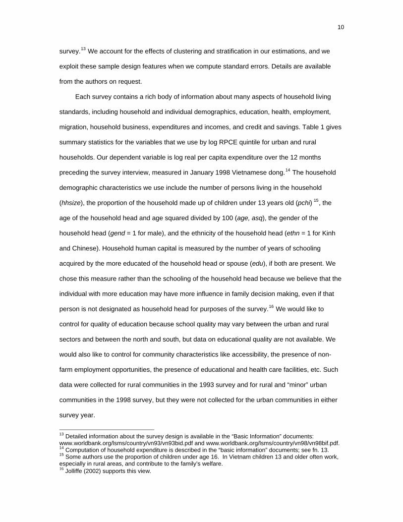
Each survey contains a rich body of information about many aspects of household living
standards, including household and individual demographics, education, health, employment,
migration, household business, expenditures and incomes, and credit and savings. Table 1 gives
summary statistics for the variables that we use by log RPCE quintile for urban and rural
households. Our dependent variable is log real per capita expenditure over the 12 months
preceding the survey interview, measured in January 1998 Vietnamese dong.14 The household
demographic characteristics we use include the number of persons living in the household
(hhsize), the proportion of the household made up of children under 13 years old (pchi) 15, the
age of the household head and age squared divided by 100 (age, asq), the gender of the
household head (gend = 1 for male), and the ethnicity of the household head (ethn = 1 for Kinh
and Chinese). Household human capital is measured by the number of years of schooling
acquired by the more educated of the household head or spouse (edu), if both are present. We
chose this measure rather than the schooling of the household head because we believe that the
individual with more education may have more influence in family decision making, even if that
person is not designated as household head for purposes of the survey.16 We would like to
control for quality of education because school quality may vary between the urban and rural
sectors and between the north and south, but data on educational quality are not available. We
would also like to control for community characteristics like accessibility, the presence of non-
farm employment opportunities, the presence of educational and health care facilities, etc. Such
data were collected for rural communities in the 1993 survey and for rural and “minor” urban
communities in the 1998 survey, but they were not collected for the urban communities in either
survey year.
13 Detailed information about the survey design is available in the “Basic Information” documents: www.worldbank.org/lsms/country/vn93/vn93bid.pdf and www.worldbank.org/lsms/country/vn98/vn98bif.pdf. 14 Computation of household expenditure is described in the “basic information” documents; see fn. 13. 15 Some authors use the proportion of children under age 16. In Vietnam children 13 and older often work, especially in rural areas, and contribute to the family’s welfare. 16 Jolliffe (2002) supports this view.
11
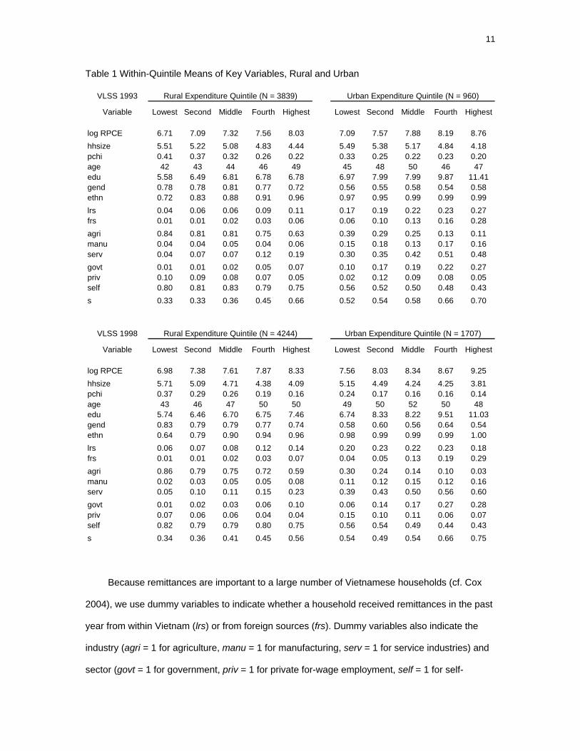
Table 1 Within-Quintile Means of Key Variables, Rural and Urban
VLSS 1993
Variable Lowest Second Middle Fourth Highest Lowest Second Middle Fourth Highest
log RPCE 6.71 7.09 7.32 7.56 8.03 7.09 7.57 7.88 8.19 8.76hhsize 5.51 5.22 5.08 4.83 4.44 5.49 5.38 5.17 4.84 4.18pchi 0.41 0.37 0.32 0.26 0.22 0.33 0.25 0.22 0.23 0.20age 42 43 44 46 49 45 48 50 46 47edu 5.58 6.49 6.81 6.78 6.78 6.97 7.99 7.99 9.87 11.41gend 0.78 0.78 0.81 0.77 0.72 0.56 0.55 0.58 0.54 0.58ethn 0.72 0.83 0.88 0.91 0.96 0.97 0.95 0.99 0.99 0.99lrs 0.04 0.06 0.06 0.09 0.11 0.17 0.19 0.22 0.23 0.27frs 0.01 0.01 0.02 0.03 0.06 0.06 0.10 0.13 0.16 0.28agri 0.84 0.81 0.81 0.75 0.63 0.39 0.29 0.25 0.13 0.11manu 0.04 0.04 0.05 0.04 0.06 0.15 0.18 0.13 0.17 0.16serv 0.04 0.07 0.07 0.12 0.19 0.30 0.35 0.42 0.51 0.48govt 0.01 0.01 0.02 0.05 0.07 0.10 0.17 0.19 0.22 0.27priv 0.10 0.09 0.08 0.07 0.05 0.02 0.12 0.09 0.08 0.05self 0.80 0.81 0.83 0.79 0.75 0.56 0.52 0.50 0.48 0.43s 0.33 0.33 0.36 0.45 0.66 0.52 0.54 0.58 0.66 0.70
VLSS 1998
Variable Lowest Second Middle Fourth Highest Lowest Second Middle Fourth Highest
log RPCE 6.98 7.38 7.61 7.87 8.33 7.56 8.03 8.34 8.67 9.25hhsize 5.71 5.09 4.71 4.38 4.09 5.15 4.49 4.24 4.25 3.81pchi 0.37 0.29 0.26 0.19 0.16 0.24 0.17 0.16 0.16 0.14age 43 46 47 50 50 49 50 52 50 48edu 5.74 6.46 6.70 6.75 7.46 6.74 8.33 8.22 9.51 11.03gend 0.83 0.79 0.79 0.77 0.74 0.58 0.60 0.56 0.64 0.54ethn 0.64 0.79 0.90 0.94 0.96 0.98 0.99 0.99 0.99 1.00lrs 0.06 0.07 0.08 0.12 0.14 0.20 0.23 0.22 0.23 0.18frs 0.01 0.01 0.02 0.03 0.07 0.04 0.05 0.13 0.19 0.29agri 0.86 0.79 0.75 0.72 0.59 0.30 0.24 0.14 0.10 0.03manu 0.02 0.03 0.05 0.05 0.08 0.11 0.12 0.15 0.12 0.16serv 0.05 0.10 0.11 0.15 0.23 0.39 0.43 0.50 0.56 0.60govt 0.01 0.02 0.03 0.06 0.10 0.06 0.14 0.17 0.27 0.28priv 0.07 0.06 0.06 0.04 0.04 0.15 0.10 0.11 0.06 0.07self 0.82 0.79 0.79 0.80 0.75 0.56 0.54 0.49 0.44 0.43s 0.34 0.36 0.41 0.45 0.56 0.54 0.49 0.54 0.66 0.75
Rural Expenditure Quintile (N = 3839) Urban Expenditure Quintile (N = 960)
Rural Expenditure Quintile (N = 4244) Urban Expenditure Quintile (N = 1707)
Because remittances are important to a large number of Vietnamese households (cf. Cox
2004), we use dummy variables to indicate whether a household received remittances in the past
year from within Vietnam (lrs) or from foreign sources (frs). Dummy variables also indicate the
industry (agri = 1 for agriculture, manu = 1 for manufacturing, serv = 1 for service industries) and
sector (govt = 1 for government, priv = 1 for private for-wage employment, self = 1 for self-

12
employment) of employment of the household head.17 We estimated our model using similar
variables for the industry and sector of employment of the household head’s spouse. The
coefficients on these variables were insignificant so we do not report these results. Finally,
dummy variables indicate whether a household is located in the north or south (s = 1 for south) or
in an urban or rural area (u = 1 for urban). We do not examine more detailed regional differences
because our main interest is in analyzing the urban-rural gap, controlling for north-south
differences; these dichotomies seem to capture the most important variations.18
Several variables exhibit interesting patterns. The average education level increases
monotonically across quintiles in both survey years and is higher in urban areas. Gender of the
household head is not correlated with income quintile, but the frequency of female-headed
households is substantially higher among urban households than among rural ones. Ethnic
minorities are rare in every urban quintile, but are over-represented in the two bottom rural
quintiles. The pattern of industry dummies suggests a strong negative relationship between
agricultural employment and log RPCE. The sectoral dummies show that the vast majority of
household heads in the rural sector are self-employed. In the urban sector a majority in the lower
quintiles is self employed as well. Finally, the representation of southern households increases
monotonically with quintile in both urban and rural households. This is not surprising, given the
usual association of “south” with “rich Ho Chi Minh City,” and the facts that industry is more
developed, agriculture is more diversified, and agricultural productivity is higher in the south.
The next section explores some of these relationships in more detail via the quantile
regression model.
17 The omitted industry and sector are made up of household heads who reported not working during the previous year. This includes unemployed individuals as well as those not in the labor force because they are retirees, stay-at-home parents designated as household head for purposes of the survey, etc. We did not use more detailed profession or industry codes for several reasons. First, our unit of observation is the household rather than the individual, and using a broad industry or sector classification for the employment of the household head may be satisfactory for classifying households by “type.” Second, the professional and industry codes were revised between the two survey years and they are difficult to match up at the disaggregate level. Third, we wanted to balance control for type of employment against the computational burden required to achieve that control. 18 Gallup (2004, page 59) finds that “[o]utside Ho Chi Minh City and Hanoi, average wages were surprisingly similar across regions in 1993, and they had become even more similar by 1998.” Benjamin and Brandt (2004) also focus on the north and south in their study of “[a]griculture and income distribution in rural Vietnam: a tale of two regions.”
13
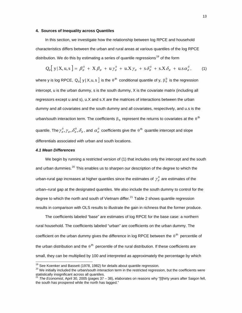
4. Sources of Inequality across Quantiles
In this section, we investigate how the relationship between log RPCE and household
characteristics differs between the urban and rural areas at various quantiles of the log RPCE
distribution. We do this by estimating a series of quantile regressions19 of the form
[ ] 0000 u.s s.X s u.X u X s u, X, |y θθθθθθθθ αδδγγββ ++++++=Q , (1)
where y is log RPCE, is the conditional quantile of y, is the regression
intercept, u is the urban dummy, s is the south dummy, X is the covariate matrix (including all
regressors except u and s), u.X and s.X are the matrices of interactions between the urban
dummy and all covariates and the south dummy and all covariates, respectively, and u.s is the
urban/south interaction term. The coefficients
[ ] s u, X, | y Qθthθ 0
θβ
θβ represent the returns to covariates at the
quantile. The , and coefficients give the quantile intercept and slope
differentials associated with urban and south locations.
thθ
θθθθ δδγγ ,,, 00 0θα thθ
4.1 Mean Differences
We begin by running a restricted version of (1) that includes only the intercept and the south
and urban dummies.20 This enables us to sharpen our description of the degree to which the
urban-rural gap increases at higher quantiles since the estimates of are estimates of the
urban–rural gap at the designated quantiles. We also include the south dummy to control for the
degree to which the north and south of Vietnam differ.
0θγ
21 Table 2 shows quantile regression
results in comparison with OLS results to illustrate the gain in richness that the former produce.
The coefficients labeled “base” are estimates of log RPCE for the base case: a northern
rural household. The coefficients labeled “urban” are coefficients on the urban dummy. The
coefficient on the urban dummy gives the difference in log RPCE between the percentile of
the urban distribution and the percentile of the rural distribution. If these coefficients are
small, they can be multiplied by 100 and interpreted as approximately the percentage by which
thθ
thθ
19 See Koenker and Bassett (1978, 1982) for details about quantile regression. 20 We initially included the urban/south interaction term in the restricted regression, but the coefficients were statistically insignificant across all quantiles. 21 The Economist, April 30, 2005 (pages 37 – 38), elaborates on reasons why “[t]hirty years after Saigon fell, the south has prospered while the north has lagged.”
14
urban households’ real per capita expenditures exceed those of rural households.22 These
coefficients are highly significant, increase across the quantiles, and are larger in 1998 than in
1993. Similarly, the coefficients labeled “south” are coefficients on the south dummy and
(multiplied by 100) indicate approximately the percentage by which southern households’ real
per-capita expenditures exceed those of northern households. Except at the 5th percentile, these
coefficients are statistically significant and they increase across the quantiles. However, the
north-south differentials are smaller in 1998 than in 1993.
Of course, the coefficients on the south and urban dummies reflect differences in
distributions of covariates and differences in the returns to those covariates. In the next
subsection, we discuss our estimates of those differences.
Table 2. Estimates of the urban-rural gap at the mean and at various quantiles.23
Year Coefficient OLS 5th 25th 50th 75th 95th
1993 base 7.25 6.62 6.98 7.24 7.51 7.96p-value (0.00) (0.00) (0.00) (0.00) (0.00) (0.00)
urban 0.52 0.34 0.42 0.51 0.59 0.74p-value (0.00) (0.00) (0.00) (0.00) (0.00) (0.00)
south 0.20 -0.02 0.15 0.22 0.29 0.36p-value (0.00) (0.83) (0.00) (0.00) (0.00) (0.00)
1998 base 7.56 6.85 7.26 7.53 7.84 8.35p-value (0.00) (0.00) (0.00) (0.00) (0.00) (0.00)
urban 0.72 0.60 0.64 0.72 0.79 0.93p-value (0.00) (0.00) (0.00) (0.00) (0.00) (0.00)
south 0.15 -0.05 0.12 0.17 0.21 0.22p-value (0.00) (0.54) (0.00) (0.00) (0.00) (0.00)
Quantiles
22 The estimated coefficients on the other variables can be similarly interpreted. The approximation to percentage differences in RPCE is poor for larger coefficient values; exact percentage differences are
( )[ ] 1 - ˆexp 100 θγ⋅ , ( )[ ] 1 - ˆexp 100 , etc. θδ⋅23 Bootstrapped standard errors were computed on 1000 replications and account for the effects of clustering and stratification. The p-values are for two-sided tests based on asymptotic standard normal distributions of the z-ratios under the null hypothesis that the corresponding coefficients are zero.
15
4.2 Quantile Regressions
We estimated the full model, including interactions of the south and urban dummies with all
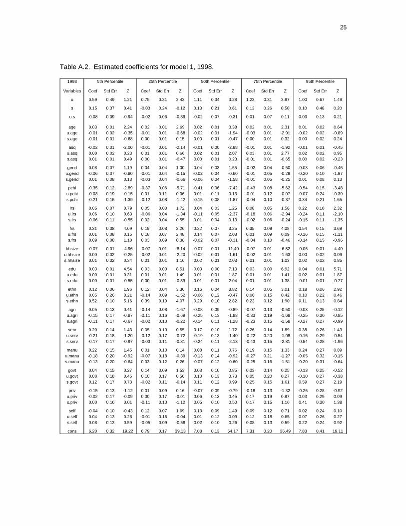
the remaining covariates, for quantiles 1 - 99. Appendix Tables A.1 and A.2 present the
coefficients and their z-ratios for quantiles 5, 25, 50, 75, and 95 for the two survey years.24
The coefficient on the urban dummy measures the urban-rural gap that is unexplained by
the covariates in the regressions. The gaps are large and are statistically significant in all but
three cases. Interestingly, after controlling for covariates, these unexplained gaps are larger than
those displayed in Table 2, particularly in 1993.
In 1998, the unexplained urban-rural gap was smaller than in 1993 at the 5th, 25th, and 50th
percentiles, and essentially the same towards the top of the distribution. The urban-rural gaps of
the North and South are virtually indistinguishable in both years, except that there was a
statistically significantly smaller gap at the 95th percentile in the South in 1993. This difference
vanished entirely by 1998. In 1993 the South was slightly better off than the North at the higher
quantiles in some way unrelated to our covariates, but this difference also vanished by 1998. The
apparent advantages of the south shown in Table 2 are almost fully explained by the covariates.
Since the unexplained urban-rural gap decreased between the two sample periods, the
increase in the gap over this period (as shown in Table 2) must be due to changes in the
distributions of covariates or their returns. Table 1 documents the changes in distributions of
covariates. The differences in returns across the distributions are shown in Tables A.1 and A.2.
Table B.1 in Appendix B shows the statistical significance of the differences in coefficients
estimated at 75th and 25th percentiles for both 1993 and 1998 for the full specification. As can be
seen from the table, many of these differences are insignificant, but about one third are significant
at the 10% level in one-tail tests, and some are quite significant. We examine in some detail the
returns to certain covariates of interest.
24 Some coefficients in some quantile regressions are statistically insignificant. However, nearly every regressor has a statistically significant coefficient at some quantile. Since we need to specify the same model for every quantile in order to perform the decomposition, we use the same specification at all quantiles.

16
4.3 Returns to education, ethnicity, and agricultural employment.25
Coefficients on several variables, like age of household head, age-squared, gender of
household head, household size, etc., do not display particularly interesting patterns across
quantiles, but some variables are worth closer inspection. In this section, we examine the returns
to education, ethnicity, and agricultural employment in each of four strata (rural North, urban
North, rural South, and urban South) in each of the two survey years.
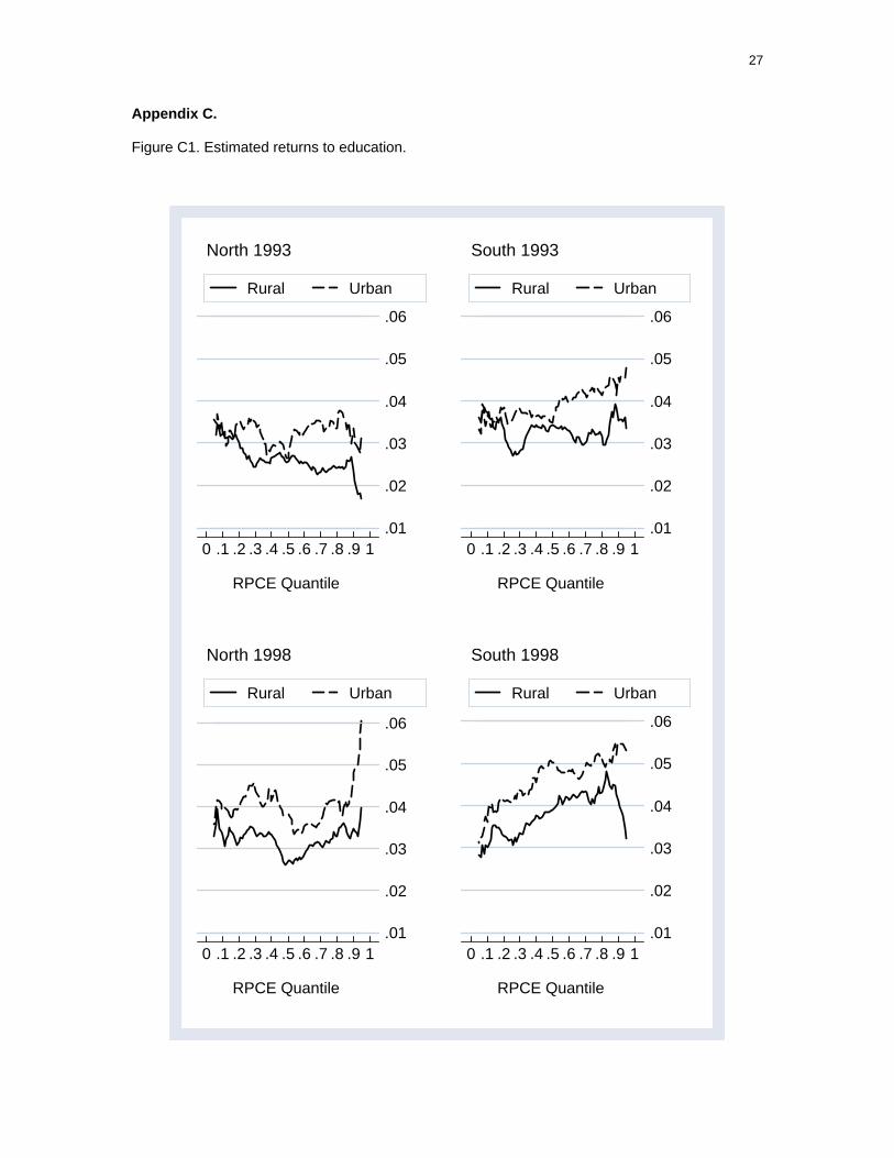
Education. Returns to education – in terms of real per-capita expenditures – are plotted in
Figure C1 in Appendix C, where the vertical axis indicates the estimated difference in log real
RPCE associated with an additional year’s education for the household head or spouse
(whichever had more education). The base case is the rural North, represented by the solid lines
in the two left-hand panels for 1993 and 1998. Returns to education are statistically significant
across all quantiles for the base case. We see in Tables A.1 and A.2 that the urban differential is
almost always positive and usually substantial, consistent with our expectation that education
pays off better in urban areas where network effects and specialization enhance the productivity
of educated individuals. Education also pays off in the South relative to the North, at the median
and above (except at the very top of the distribution in 1998), and probably for the same reasons:
the South accounts for the lion’s share of sophisticated market activity in Vietnam (manufacturing
and business services), and in addition, has more historical experience with market institutions
and less historical experience with central planning.
The patterns of returns to education across the quantiles vary between the North and
South. The returns to education show a marked increase at the upper quantiles in the South in
1993 for urban households. A comparable pattern is not seen in the North. In 1998, the upward
sloping returns to education in the South are evident in both the urban and rural sectors. The
North in 1998 continues to show a more stable pattern of returns across the quantiles with a huge
25 The results discussed in this section are illustrated by Figures C1 – C3 in Appendix C. The return to each covariate in the urban North was calculated by adding the urban differential to the (base case) coefficient on the covariate; the return to that covariate in the rural South was calculated by adding the south differential to the base case coefficient; the returns to the covariate in the urban South was calculated by adding the urban differential and the south differential to the base case coefficient. The figures plot these returns against log RPCE percentile for percentiles from the 5th to the 95th in one-percent increments. Assessments of statistical significance are drawn from Tables A1 and A2, but these pertain only to the 5th, 25th, 50th, 75th, and 95th percentiles.
17
blip up for the very top urban households. Finally, returns to education increased, most
substantially in the South, over the five-year period covered by our data.
Ethnicity. Returns to belonging to the ethnic majority vary by quantile and year, as
shown in Figure C.2. In 1993, the base returns to ethnicity (in the rural north) were small (ranging
from approximately 0.04 to 0.11) and statistically significant at the 75th and 95th percentiles.
Surprisingly, the urban differentials were negative (Table A.1 shows that the urban-rural
differences in log RPCE ranged from -0.48 to -0.03) and statistically significant except at the top
of the distribution. The south differentials ranged from 0.23 to 0.56 and were statistically
significant across the entire welfare distribution, with the differentials being largest at the low end
of the distribution. The net effect is that non-minority rural southerners were significantly better
off, controlling for other factors.
In 1998, the base returns to ethnicity ranged from approximately 0.12 to 0.18 and were
highly significant, but the urban differentials had become statistically insignificant. The south
differentials remained positive (from 0.11 to 0.52) and statistically significant, except at the top of
the distribution. Again, the largest differentials were at the low end of the distribution. The net
effect in 1998 was that Kinh and Chinese southerners were better off than minority southerners
and better off than majority northerners.
Agriculture. In 1993, rural northern households engaged in agriculture were better off at
the low end of the distribution, about the same at the median, and worse off at the high end of the
distribution than their neighbors engaged in other industries; see Table A.1 and Figure C.3. The
urban differential accentuated this trend but was not statistically significant; the south differential
was also negative (except for being positive at the very top of the distribution) and insignificant.
By 1998, the monotonic relationship between the agriculture coefficient and quantile had
vanished, and rural northern households engaging in agriculture were not statistically significantly
distinguishable from households in other industries. In 1998 both the urban and south differentials
were negative and generally decreasing with quantile, but they were not statistically significant.
On net, in 1998, the penalty for engaging in agricultural employment was strongest for southern
urban households at about the third quartile of the welfare distribution.
18
One important aspect of economic development is the generation of non-agricultural
employment to absorb labor shed by the agricultural sector as labor productivity rises there. It
seems that we have indirect evidence that these transformations are not occurring rapidly enough
in Vietnam on average.
The marginal effects discussed in this section vary across quantiles and over time. In
addition, inspection of Table 1 reveals that changes in covariate distributions across quantiles
between 1993 and 1998 are small compared to urban-rural differences. To summarize the effects
of covariates and returns to covariates on the size and change in the urban-rural gap, we now
turn to the Machado-Mata (2005) decomposition.
5. The Decomposition
In the previous section, we discussed the fact that returns to certain characteristics vary
systematically across conditional quantiles of the distribution of log RPCE and also differ between
the urban and rural sectors. It is also the case that the distributions of covariates differ between
the two sectors. The Machado-Mata technique enables us to decompose the urban-rural gap at
each quantile into two components: one component due to urban-rural differences in the
distributions of returns and one component due to differences in the distributions of covariates
between urban and rural households. The decomposition is based on the construction of a
counterfactual distribution of log RPCE for rural households. This counterfactual distribution of
rural log RPCE is the distribution of log RPCE that would have prevailed if rural households had
been endowed with urban characteristics but received rural returns to those characteristics. We
denote the counterfactual distribution by ( ) b , Z | y F RU∗ where y is log RPCE, Z is the
distribution of covariates, and b is the collection of vectors of quantile regression coefficients
(returns) at the various quantiles. Superscripts U and R designate urban and rural values and the
asterisk designates generated values.
( ) b , Z | y F RU∗ is constructed using the Machado-Mata algorithm as follows. First, for
each quantile θ = 0.01, 0.02, …, 0.99, estimate the quantile regression coefficients using ( ) bR θ
19
the rural data. Second, use the urban data to generate fitted values ( ) )(b Z RU θθ =∗y . For
each this generates Nθ U fitted values, where NU is the size of the urban sub-sample. Next,
randomly select s = 100 of the elements of ( ) y θ∗ for each θ and stack these into a 99 x 100
element vector The empirical CDF of these values is the estimated counterfactual
distribution.
.y∗
The decomposition compares the counterfactual distribution with the empirical urban and
rural log RPCE distributions. Define the quantiles of these distributions by , ,
and , respectively. The difference between the quantile of the urban and rural
distributions is
thθ ( ) y θ∗ ( ) yU θ
( ) yR θ thθ
( ) ( ) ( ) ( ){ } ( ) ( ){ } y - y y - y y - y RURU θθ+θθ=θθ ∗∗ . (2)
The first term on the right-hand side is the returns effect: it measures the contribution of the
difference in returns to the urban-rural gap at the quantile. The second term on the right-hand
side is the covariate effect: it measures the contribution of the different covariate values to the
urban-rural gap at the quantile. By randomly re-sampling the rural data, we computed
bootstrapped standard errors for the estimated returns and covariate effects; details are available
on request.
thθ
thθ
20
0
.2
.4
.6
Diff
eren
ce in
log
RP
CE
0 20 40 60 80 100Percentile
Returns Effect 1993Covariate Effect 1993
Source: Authors' calculations.
0
.2
.4
.6
Diff
eren
ce in
log
RP
CE
0 20 40 60 80 100Percentile
Returns Effect 1998Covariate Effect 1998
Source: Authors' calculations.
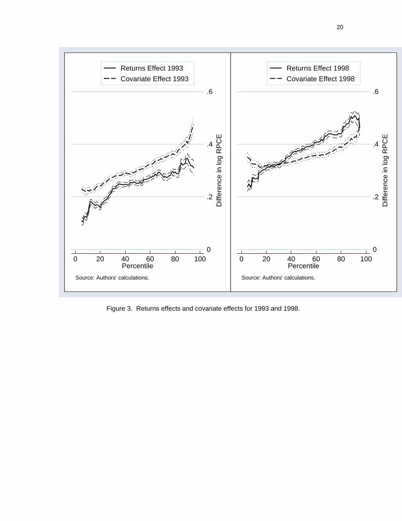
Figure 3. Returns effects and covariate effects for 1993 and 1998.

21
Figure 3 shows the returns effects and covariate effects for 1993 and 1998 for quantiles 5 to
95, with 95% confidence bounds. Three features of these graphs stand out. First, covariate
effects and returns effects are both larger at higher quantiles, resulting in a larger urban-rural gap
at higher quantiles. Second, the magnitude of the returns effects increased dramatically between
1993 and 1998. This feature is consistent with the increased marketization flowing from the doi
moi reforms. Third, the slope of the returns effects generally increased between the two surveys,
indicating that returns contributed proportionately more to the increase in the gap at higher
quantiles. Similarly the slope of the covariate effects generally decreased between the two
surveys.
The dominance of covariate effects at the lower end of the distributions in 1998 means that
for the poorest households, differences in household characteristics matter more than differences
in returns to those characteristics. This probably reflects the fact that the poor typically work in
jobs that pay little above the subsistence level, so urban–rural variation in market returns is not
important at the bottom of the distribution. On the other hand, the dominance of the returns
effects over the covariate effects at the top of the distributions means that for the most well-off
households, urban markets pay more for their attributes than rural markets would. That is, even
though the urban households have superior characteristics, the welfare gap is caused primarily
by the differences in returns.
6. Conclusions
In this paper we use a quantile regression decomposition method to analyze the sources of
urban-rural household welfare inequality in Vietnam. Specifically, we decompose the urban-rural
log RPCE gap across the distribution into two components: one due to differences in household
characteristics and one due to differences in returns to those characteristics.
The covariate and returns effects are both larger at the top of the log RPCE distribution than
at the bottom in both survey years, as is the urban-rural gap. We also find that the magnitude of
the returns effects increased dramatically between 1993 and 1998, reflecting the increased
marketization associated with the doi moi reforms. One particular example of increased returns is
22
the returns to education. In addition, the slope of the returns effect increased between the two
surveys indicating that this effect was proportionately stronger at higher quantiles of the log
RPCE distribution. Since the same was not true of the covariate effects, we find that in 1998, the
covariate effects dominate at the bottom of the distribution, while the returns effects strongly and
increasingly dominate towards the top of the distribution. In other words, for the poor, what makes
urban households better off than their rural counterparts in 1998 is due more to the difference
between urban and rural household characteristics, whereas for the better-off households, the
difference is due primarily to the difference between urban and rural rewards for their
characteristics.
These results are consistent with the type of reforms that were instituted in Vietnam.
Households with greater human capital (e.g., education) endowments benefited more from the
reforms because the returns to their endowments changed. The results for 1993 show that the
urban sector was much better endowed than the rural sector and this explains most of the gap at
that time. The results for 1998 show that there was a much larger change in returns in the urban
sector and this, combined with the difference in endowments, explains most of the widening
urban-rural gap. Our results may indicate an urban bias in development policy; more likely, they
simply reflect the fact that households in the urban areas were better able to take advantage of
the liberalization introduced by the doi moi reforms.
What do our results suggest about policy interventions? Generally, our results support
conventional approaches to poverty reduction and to reducing the urban-rural welfare gap.
Policies can be dichotomized according to whether they improve households’ endowments of
marketable characteristics and employment opportunities or whether they improve returns to
those characteristics and opportunities. Since it is the endowment of marketable characteristics
that matters more (relative to market returns) for those at the lower end of the welfare distribution,
policies for reducing rural poverty and the urban-rural gap are naturally more effective when they
include education and employment opportunities for the poor, particularly those in rural areas.
Family planning, through its likely effect on the proportion of children in the household, would also

23
have a strong effect. Since relatively rich households can afford investments in education and
family planning, the case can be made to subsidize these investments for the poor.
The urban-rural disparity in returns to characteristics is best addressed by enhanced labor
market flexibility and investments in infrastructure in rural areas. This would allow labor to migrate
to the region or sector that provides the best labor market returns, while supporting increased
labor productivity in rural areas. In addition, we have strong evidence that ethnic minority status
matters a great deal, even after controlling for other covariates. Moreover, the penalty for minority
status in Vietnam increased over the 1993 – 1998 period and minority representation in the
lowest rural welfare quintile increased. Policies that decrease the penalty associated with minority
status in rural Vietnam would have a significant impact.
24
Appendix A.
Table A.1. Estimated coefficients for model 1, 1993.
1993
Variables Coef Std Err Z Coef Std Err Z Coeff Std Err Z Coeff Std Err Z Coef Std Err Z
u 1.80 0.61 2.96 1.04 0.38 2.73 1.21 0.35 3.48 1.23 0.44 2.76 1.04 0.76 1.38
s -0.23 0.41 -0.56 -0.02 0.27 -0.09 0.16 0.25 0.63 0.45 0.25 1.77 0.53 0.37 1.42
u.s -0.04 0.11 -0.33 0.06 0.09 0.61 -0.04 0.08 -0.54 -0.07 0.09 -0.74 -0.26 0.13 -2.05
age 0.01 0.01 1.58 0.02 0.01 2.85 0.01 0.01 1.99 0.02 0.01 3.22 0.03 0.01 2.73u.age -0.03 0.02 -1.40 -0.01 0.01 -0.81 -0.01 0.01 -1.24 -0.02 0.02 -1.20 -0.02 0.02 -0.84s.age 0.01 0.01 0.38 0.00 0.01 -0.08 0.00 0.01 -0.08 -0.02 0.01 -1.62 -0.02 0.02 -1.57
asq -0.01 0.01 -1.02 -0.02 0.01 -2.28 -0.01 0.01 -1.42 -0.01 0.01 -2.41 -0.03 0.01 -2.46u.asq 0.02 0.02 1.18 0.01 0.01 0.67 0.01 0.01 1.09 0.02 0.02 1.06 0.02 0.02 0.88s.asq -0.01 0.01 -0.59 0.00 0.01 0.00 0.00 0.01 -0.07 0.02 0.01 1.55 0.03 0.02 1.68
gend 0.08 0.04 2.12 0.04 0.03 1.16 0.02 0.03 0.79 0.01 0.03 0.29 -0.06 0.06 -1.10u.gend -0.12 0.09 -1.30 -0.05 0.07 -0.79 0.04 0.05 0.83 0.07 0.07 1.04 0.09 0.10 0.88s.gend 0.00 0.07 0.04 0.06 0.05 1.14 -0.03 0.04 -0.68 -0.05 0.05 -1.10 -0.07 0.10 -0.75
pchi -0.45 0.10 -4.30 -0.44 0.07 -6.79 -0.47 0.06 -7.97 -0.39 0.06 -6.85 -0.28 0.11 -2.62u.pchi -0.01 0.26 -0.05 -0.15 0.19 -0.76 -0.04 0.13 -0.28 -0.16 0.18 -0.86 -0.28 0.29 -0.94s.pchi -0.19 0.17 -1.16 -0.09 0.12 -0.79 -0.09 0.10 -0.89 -0.17 0.12 -1.49 -0.13 0.17 -0.75
lrs 0.09 0.06 1.42 0.04 0.04 1.17 0.05 0.03 1.50 -0.01 0.04 -0.33 0.20 0.12 1.69u.lrs 0.07 0.11 0.64 -0.01 0.07 -0.11 -0.07 0.06 -1.15 -0.08 0.07 -1.12 -0.07 0.14 -0.51s.lrs -0.08 0.09 -0.85 -0.04 0.06 -0.71 -0.07 0.06 -1.21 -0.03 0.06 -0.40 -0.30 0.14 -2.22
frs 0.18 0.09 1.91 0.17 0.09 1.84 0.20 0.07 2.82 0.32 0.08 4.00 0.51 0.18 2.83u.frs -0.15 0.16 -0.95 0.06 0.10 0.59 0.10 0.13 0.76 0.17 0.13 1.25 0.00 0.17 0.00s.frs 0.09 0.12 0.75 -0.04 0.11 -0.38 -0.05 0.12 -0.45 -0.02 0.13 -0.19 -0.02 0.19 -0.12
hhsize -0.04 0.01 -4.21 -0.03 0.01 -3.75 -0.03 0.01 -4.59 -0.05 0.01 -7.66 -0.06 0.01 -4.52u.hhsize -0.02 0.02 -1.00 -0.03 0.01 -2.05 -0.03 0.01 -2.10 -0.02 0.01 -1.68 -0.02 0.02 -0.69s.hhsize 0.01 0.01 0.61 0.00 0.01 0.38 0.00 0.01 -0.26 0.02 0.01 2.03 0.03 0.02 1.55
edu 0.04 0.01 5.51 0.03 0.00 5.54 0.03 0.00 6.75 0.02 0.00 6.21 0.02 0.01 2.41u.edu 0.00 0.01 -0.33 0.01 0.01 1.15 0.00 0.01 0.10 0.01 0.01 1.51 0.01 0.01 1.27s.edu 0.00 0.01 0.06 0.00 0.01 0.21 0.01 0.01 1.68 0.01 0.01 1.51 0.02 0.01 1.56
ethn 0.04 0.06 0.72 0.08 0.06 1.34 0.04 0.04 1.00 0.08 0.04 2.14 0.11 0.06 1.94u.ethn -0.48 0.20 -2.41 -0.24 0.13 -1.82 -0.30 0.15 -2.00 -0.22 0.13 -1.62 0.03 0.34 0.08s.ethn 0.56 0.29 1.93 0.36 0.13 2.66 0.32 0.11 2.96 0.25 0.09 2.73 0.23 0.13 1.78
agri 0.23 0.13 1.75 0.14 0.10 1.41 -0.01 0.07 -0.21 -0.10 0.08 -1.24 -0.35 0.09 -3.70u.agri 0.10 0.22 0.43 -0.12 0.18 -0.69 -0.09 0.15 -0.59 -0.22 0.24 -0.93 -0.36 0.26 -1.40s.agri -0.14 0.20 -0.67 -0.08 0.15 -0.55 -0.17 0.12 -1.41 -0.08 0.21 -0.37 0.25 0.20 1.26
serv 0.43 0.13 3.22 0.35 0.10 3.42 0.20 0.08 2.63 0.14 0.10 1.40 -0.12 0.13 -0.90u.serv 0.19 0.24 0.78 -0.09 0.19 -0.48 -0.03 0.14 -0.19 -0.13 0.23 -0.58 -0.22 0.27 -0.83s.serv -0.25 0.21 -1.16 -0.15 0.17 -0.87 -0.25 0.12 -2.07 -0.16 0.21 -0.78 0.22 0.23 0.97
manu 0.40 0.14 2.83 0.18 0.11 1.62 0.08 0.09 0.93 0.04 0.10 0.35 -0.24 0.13 -1.82u.manu 0.06 0.27 0.21 -0.08 0.19 -0.40 0.00 0.16 -0.03 -0.08 0.24 -0.34 -0.21 0.28 -0.73s.manu -0.24 0.23 -1.05 -0.01 0.17 -0.05 -0.06 0.13 -0.43 -0.01 0.23 -0.05 0.36 0.24 1.52
govt -0.33 0.19 -1.77 0.01 0.12 0.08 0.14 0.07 1.93 0.11 0.09 1.22 0.26 0.16 1.69u.govt -0.38 0.27 -1.39 -0.16 0.17 -0.98 -0.24 0.13 -1.76 -0.16 0.22 -0.73 -0.14 0.28 -0.52s.govt 0.26 0.26 1.02 0.06 0.16 0.37 0.07 0.12 0.59 0.15 0.20 0.77 -0.12 0.24 -0.49
priv -0.22 0.11 -1.99 -0.13 0.10 -1.36 0.04 0.06 0.65 0.01 0.09 0.12 0.39 0.15 2.66u.priv -0.46 0.23 -2.01 -0.13 0.17 -0.77 -0.10 0.14 -0.73 -0.06 0.22 -0.28 0.07 0.25 0.26s.priv 0.04 0.19 0.22 -0.12 0.14 -0.86 -0.15 0.10 -1.46 -0.12 0.20 -0.62 -0.58 0.24 -2.44
self -0.14 0.10 -1.51 -0.09 0.08 -1.15 0.01 0.04 0.28 0.07 0.06 1.16 0.23 0.07 3.31u.self -0.37 0.20 -1.82 -0.09 0.14 -0.69 -0.13 0.12 -1.04 0.02 0.21 0.10 0.11 0.24 0.44s.self 0.00 0.18 0.03 0.02 0.12 0.17 0.12 0.09 1.32 0.10 0.19 0.53 -0.17 0.18 -0.91
cons 6.18 0.15 39.93 6.50 0.15 44.09 6.93 0.15 46.33 7.16 0.12 60.45 7.51 0.22 33.85
95th Percentile5th Percentile 25th Percentile 50th Percentile 75th Percentile
25
Table A.2. Estimated coefficients for model 1, 1998.
1998
Variables Coef Std Err Z Coef Std Err Z Coef Std Err Z Coef Std Err Z Coef Std Err Z
u 0.59 0.49 1.21 0.75 0.31 2.43 1.11 0.34 3.28 1.23 0.31 3.97 1.00 0.67 1.49
s 0.15 0.37 0.41 -0.03 0.24 -0.12 0.13 0.21 0.61 0.13 0.26 0.50 0.10 0.48 0.20
u.s -0.08 0.09 -0.94 -0.02 0.06 -0.39 -0.02 0.07 -0.31 0.01 0.07 0.11 0.03 0.13 0.21
age 0.03 0.01 2.24 0.02 0.01 2.69 0.02 0.01 3.38 0.02 0.01 2.31 0.01 0.02 0.64u.age -0.01 0.02 -0.35 -0.01 0.01 -0.68 -0.02 0.01 -1.94 -0.03 0.01 -2.91 -0.02 0.02 -0.89s.age -0.01 0.01 -0.68 0.00 0.01 0.15 0.00 0.01 -0.47 0.00 0.01 0.32 0.00 0.02 0.24
asq -0.02 0.01 -2.00 -0.01 0.01 -2.14 -0.01 0.00 -2.88 -0.01 0.01 -1.92 -0.01 0.01 -0.45u.asq 0.00 0.02 0.23 0.01 0.01 0.66 0.02 0.01 2.07 0.03 0.01 2.77 0.02 0.02 0.95s.asq 0.01 0.01 0.49 0.00 0.01 -0.47 0.00 0.01 0.23 -0.01 0.01 -0.65 0.00 0.02 -0.23
gend 0.08 0.07 1.19 0.04 0.04 1.00 0.04 0.03 1.55 -0.02 0.04 -0.50 -0.03 0.06 -0.46u.gend -0.06 0.07 -0.80 -0.01 0.04 -0.15 -0.02 0.04 -0.60 -0.01 0.05 -0.29 -0.20 0.10 -1.97s.gend 0.01 0.08 0.13 -0.03 0.04 -0.66 -0.06 0.04 -1.58 -0.01 0.05 -0.25 0.01 0.08 0.13
pchi -0.35 0.12 -2.89 -0.37 0.06 -5.71 -0.41 0.06 -7.42 -0.43 0.08 -5.62 -0.54 0.15 -3.48u.pchi -0.03 0.19 -0.15 0.01 0.11 0.06 0.01 0.11 0.13 -0.01 0.12 -0.07 -0.07 0.24 -0.30s.pchi -0.21 0.15 -1.39 -0.12 0.08 -1.42 -0.15 0.08 -1.87 -0.04 0.10 -0.37 0.34 0.21 1.65
lrs 0.05 0.07 0.79 0.05 0.03 1.72 0.04 0.03 1.25 0.08 0.05 1.56 0.22 0.10 2.32u.lrs 0.06 0.10 0.63 -0.06 0.04 -1.34 -0.11 0.05 -2.37 -0.18 0.06 -2.94 -0.24 0.11 -2.10s.lrs -0.06 0.11 -0.55 0.02 0.04 0.55 0.01 0.04 0.13 -0.02 0.06 -0.24 -0.15 0.11 -1.35
frs 0.31 0.08 4.09 0.19 0.08 2.26 0.22 0.07 3.25 0.35 0.09 4.08 0.54 0.15 3.69u.frs 0.01 0.08 0.15 0.18 0.07 2.48 0.14 0.07 2.08 0.01 0.09 0.09 -0.16 0.15 -1.11s.frs 0.09 0.08 1.10 0.03 0.09 0.38 -0.02 0.07 -0.31 -0.04 0.10 -0.46 -0.14 0.15 -0.96
hhsize -0.07 0.01 -4.96 -0.07 0.01 -8.14 -0.07 0.01 -11.40 -0.07 0.01 -6.82 -0.06 0.01 -4.40u.hhsize 0.00 0.02 -0.25 -0.02 0.01 -2.20 -0.02 0.01 -1.61 -0.02 0.01 -1.63 0.00 0.02 0.09s.hhsize 0.01 0.02 0.34 0.01 0.01 1.16 0.02 0.01 2.03 0.01 0.01 1.03 0.02 0.02 0.85
edu 0.03 0.01 4.54 0.03 0.00 8.51 0.03 0.00 7.10 0.03 0.00 6.92 0.04 0.01 5.71u.edu 0.00 0.01 0.31 0.01 0.01 1.49 0.01 0.01 1.87 0.01 0.01 1.41 0.02 0.01 1.87s.edu 0.00 0.01 -0.55 0.00 0.01 -0.39 0.01 0.01 2.04 0.01 0.01 1.38 -0.01 0.01 -0.77
ethn 0.12 0.06 1.96 0.12 0.04 3.36 0.16 0.04 3.82 0.14 0.05 3.01 0.18 0.06 2.92u.ethn 0.05 0.26 0.21 -0.14 0.09 -1.52 -0.06 0.12 -0.47 0.06 0.15 0.42 0.10 0.22 0.46s.ethn 0.52 0.10 5.16 0.39 0.10 4.07 0.29 0.10 2.82 0.23 0.12 1.90 0.11 0.13 0.84
agri 0.05 0.13 0.41 -0.14 0.08 -1.67 -0.08 0.09 -0.89 -0.07 0.13 -0.50 -0.03 0.25 -0.12u.agri -0.15 0.17 -0.87 -0.11 0.16 -0.69 -0.25 0.13 -1.88 -0.33 0.19 -1.68 -0.25 0.30 -0.85s.agri -0.11 0.17 -0.67 -0.02 0.10 -0.22 -0.14 0.11 -1.28 -0.23 0.15 -1.58 -0.27 0.27 -0.99
serv 0.20 0.14 1.43 0.05 0.10 0.55 0.17 0.10 1.72 0.26 0.14 1.89 0.38 0.26 1.43u.serv -0.21 0.18 -1.20 -0.12 0.17 -0.72 -0.19 0.13 -1.40 -0.22 0.20 -1.08 -0.16 0.29 -0.54s.serv -0.17 0.17 -0.97 -0.03 0.11 -0.31 -0.24 0.11 -2.13 -0.43 0.15 -2.81 -0.54 0.28 -1.96
manu 0.22 0.15 1.45 0.01 0.10 0.14 0.08 0.11 0.76 0.19 0.15 1.33 0.24 0.27 0.89u.manu -0.18 0.20 -0.92 -0.07 0.18 -0.39 -0.13 0.14 -0.92 -0.27 0.21 -1.27 -0.05 0.32 -0.15s.manu -0.13 0.20 -0.64 0.03 0.12 0.26 -0.07 0.12 -0.60 -0.25 0.16 -1.51 -0.20 0.31 -0.64
govt 0.04 0.15 0.27 0.14 0.09 1.53 0.08 0.10 0.85 0.03 0.14 0.25 -0.13 0.25 -0.52u.govt 0.08 0.18 0.45 0.10 0.17 0.56 0.10 0.13 0.73 0.05 0.20 0.27 -0.10 0.27 -0.38s.govt 0.12 0.17 0.73 -0.02 0.11 -0.14 0.11 0.12 0.99 0.25 0.15 1.61 0.59 0.27 2.19
priv -0.15 0.13 -1.12 0.01 0.09 0.16 -0.07 0.09 -0.79 -0.18 0.13 -1.32 -0.26 0.28 -0.92u.priv -0.02 0.17 -0.09 0.00 0.17 -0.01 0.06 0.13 0.45 0.17 0.19 0.87 0.03 0.29 0.09s.priv 0.00 0.16 0.01 -0.11 0.10 -1.12 0.05 0.10 0.50 0.17 0.15 1.16 0.41 0.30 1.38
self -0.04 0.10 -0.43 0.12 0.07 1.69 0.13 0.09 1.49 0.09 0.12 0.71 0.02 0.24 0.10u.self 0.04 0.13 0.28 -0.01 0.16 -0.04 0.01 0.12 0.09 0.12 0.18 0.65 0.07 0.26 0.27s.self 0.08 0.13 0.59 -0.05 0.09 -0.58 0.02 0.10 0.26 0.08 0.13 0.59 0.22 0.24 0.92
cons 6.20 0.32 19.22 6.79 0.17 39.13 7.08 0.13 54.17 7.31 0.20 36.49 7.83 0.41 19.11
75th Percentile 95th Percentile5th Percentile 25th Percentile 50th Percentile

26
Appendix B.
Table B.1. Differences between coefficients estimated at 75th and 25th percentiles, standard
errors of the differences, and z-ratios of the differences.
Diff Std Err Z Diff Std Err Z
u 0.1865 0.5158 0.3616 0.4778 0.3662 1.3048
s 0.4715 0.2884 1.6348 0.1582 0.2911 0.5435
u.s -0.1261 0.0782 -1.6132 0.0319 0.0625 0.5101
age -0.0016 0.0065 -0.2537 -0.0002 0.0084 -0.0261u.age -0.0085 0.0179 -0.4750 -0.0204 0.0127 -1.6036s.age -0.0161 0.0114 -1.4088 0.0017 0.0111 0.1564
asq 0.0027 0.0070 0.3835 -0.0005 0.0081 -0.0655u.asq 0.0081 0.0173 0.4644 0.0192 0.0125 1.5312s.asq 0.0164 0.0117 1.4044 -0.0020 0.0110 -0.1828
gend -0.0299 0.0334 -0.8948 -0.0550 0.0426 -1.2914u.gend 0.1217 0.0721 1.6886 -0.0073 0.0557 -0.1316s.gend -0.1166 0.0561 -2.0775 0.0159 0.0540 0.2951
pchi 0.0517 0.0709 0.7295 -0.0590 0.0851 -0.6936u.pchi -0.0105 0.2190 -0.0480 -0.0142 0.1360 -0.1043s.pchi -0.0793 0.1281 -0.6189 0.0786 0.1068 0.7355
lrs -0.0578 0.0471 -1.2273 0.0257 0.0498 0.5170u.lrs -0.0674 0.0804 -0.8377 -0.1239 0.0615 -2.0139s.lrs 0.0194 0.0719 0.2697 -0.0374 0.0609 -0.6141
frs 0.1503 0.1094 1.3734 0.1613 0.1038 1.5545u.frs 0.1054 0.1354 0.7788 -0.1744 0.0966 -1.8057s.frs 0.0183 0.1376 0.1330 -0.0775 0.1130 -0.6853
hhsize -0.0204 0.0079 -2.5951 -0.0004 0.0102 -0.0345u.hhsize 0.0045 0.0154 0.2920 0.0000 0.0145 -0.0030s.hhsize 0.0198 0.0128 1.5513 0.0022 0.0134 0.1627
edu -0.0024 0.0044 -0.5602 -0.0029 0.0046 -0.6366u.edu 0.0019 0.0077 0.2526 0.0011 0.0077 0.1408s.edu 0.0073 0.0067 1.0893 0.0113 0.0068 1.6551
ethn 0.0006 0.0450 0.0144 0.0133 0.0383 0.3459u.ethn 0.0242 0.1718 0.1406 0.2032 0.1577 1.2885s.ethn -0.1026 0.1052 -0.9748 -0.1645 0.1009 -1.6303
agri -0.2432 0.0999 -2.4344 0.0689 0.1372 0.5022u.agri -0.0967 0.2844 -0.3398 -0.2157 0.1922 -1.1218s.agri 0.0039 0.2265 0.0173 -0.2103 0.1547 -1.3591
serv -0.2088 0.1143 -1.8259 0.2032 0.1412 1.4390u.serv -0.0436 0.2870 -0.1520 -0.0963 0.2033 -0.4736s.serv -0.0198 0.2395 -0.0828 -0.3952 0.1591 -2.4841
manu -0.1466 0.1127 -1.3009 0.1807 0.1514 1.1941u.manu -0.0049 0.2969 -0.0164 -0.1967 0.2179 -0.9030s.manu -0.0036 0.2464 -0.0148 -0.2785 0.1711 -1.6278
govt 0.1000 0.1254 0.7976 -0.1097 0.1357 -0.8084u.govt 0.0048 0.2745 0.0173 -0.0417 0.2047 -0.2037s.govt 0.0932 0.2416 0.3859 0.2601 0.1534 1.6956
priv 0.1401 0.1090 1.2857 -0.1895 0.1295 -1.4630u.priv 0.0665 0.2771 0.2400 0.1694 0.2066 0.8199s.priv -0.0043 0.2256 -0.0191 0.2813 0.1534 1.8341
self 0.1661 0.0804 2.0655 -0.0367 0.1238 -0.2962u.self 0.1156 0.2535 0.4560 0.1260 0.1880 0.6701s.self 0.0798 0.2109 0.3786 0.1298 0.1357 0.9561
cons 0.6625 0.1429 4.6348 0.5162 0.2181 2.3669
1993 1998
27
Appendix C.
Figure C1. Estimated returns to education.
.01
.02
.03
.04
.05
.06
0 .1 .2 .3 .4 .5 .6 .7 .8 .9 1
Rural Urban
RPCE Quantile
North 1993
.01
.02
.03
.04
.05
.06
0 .1 .2 .3 .4 .5 .6 .7 .8 .9 1
Rural Urban
RPCE Quantile
South 1993
.01
.02
.03
.04
.05
.06
0 .1 .2 .3 .4 .5 .6 .7 .8 .9 1
Rural Urban
RPCE Quantile
North 1998
.01
.02
.03
.04
.05
.06
0 .1 .2 .3 .4 .5 .6 .7 .8 .9 1
Rural Urban
RPCE Quantile
South 1998

28
Figure C2. Returns to ethnicity.
-.5
0
.5
1
0 .1 .2 .3 .4 .5 .6 .7 .8 .9 1
Rural Urban
RPCE Quantile
North 1993
-.5
0
.5
1
0 .1 .2 .3 .4 .5 .6 .7 .8 .9 1
Rural Urban
RPCE Quantile
South 1993
-.5
0
.5
1
0 .1 .2 .3 .4 .5 .6 .7 .8 .9 1
Rural Urban
RPCE Quantile
North 1998
-.5
0
.5
1
0 .1 .2 .3 .4 .5 .6 .7 .8 .9 1
Rural Urban
RPCE Quantile
South 1998

29
Figure C3. Returns to agricultural employment.
-1
-.5
0
.5
0 .1 .2 .3 .4 .5 .6 .7 .8 .9 1
Rural Urban
RPCE Quantile
North 1993
-1
-.5
0
.5
0 .1 .2 .3 .4 .5 .6 .7 .8 .9 1
Rural Urban
RPCE Quantile
South 1993
-1
-.5
0
.5
0 .1 .2 .3 .4 .5 .6 .7 .8 .9 1
Rural Urban
RPCE Quantile
North 1998
-1
-.5
0
.5
0 .1 .2 .3 .4 .5 .6 .7 .8 .9 1
Rural Urban
RPCE Quantile
South 1998
30
References
1. Albrecht, J., Björklund, A., and Vroman, S. 2003. Is there a glass ceiling in Sweden? Journal of Labor Economics 21, No. 1, 145-77.
2. Asian Development Bank, 2004. Poverty Profile of the People’s Republic of China, Manila,
The Philippines. 3. Benjamin, D., and Brandt, L., 2004. Agriculture and income distribution in rural Vietnam under
economic reforms: a tale of two regions, in Glewwe, P., Agrawal, N., and Dollar, D., eds. Economic Growth, Poverty, and Household Welfare in Vietnam, World Bank, Washington, D.C.
4. Bui, Q., Cao, N., Nguyen, D., Tran, P., Haughton, D., and Haughton, J., 2001. Education and
Income in Haughton, Haughton, and Nguyen, eds., Living standards during an economic boom; the case of Vietnam, Statistical Publishing House, Hanoi.
5. Cox, D., 2004. Private interhousehold transfers in Vietnam, in Glewwe, P., Agrawal, N., and
Dollar, D., eds. Economic Growth, Poverty, and Household Welfare in Vietnam, World Bank, Washington, D.C.
6. Deaton, A. 1997. The analysis of household surveys: A microeconometric approach to
development policy, Johns Hopkins University Press, Baltimore, MD. 7. Do, Q., and Iyer, L. 2003. Land rights and economic development: evidence from Vietnam,
Policy Research Working Paper No. 3120, World Bank. 8. Dollar, D., Glewwe, P., and Litvack, J., eds., 1998. Household welfare and Vietnam’s
transition, World Bank, Washington, D.C. 9. Dollar, D., and Litvak, J., 1998. Macroeconomic reform and poverty reduction in Vietnam, in
Household welfare and Vietnam’s transition, World Bank, Washington, D.C. 10. Economist, April 30, 2005, Des McSweeney Publishers, London. 11. Gallup, J., 2004. The wage labor market and inequality in Vietnam, in Glewwe, P., Agrawal,
N., and Dollar, D., eds. Economic Growth, Poverty, and Household Welfare in Vietnam, World Bank, Washington, D.C.
12. General Statistical Office of Vietnam, 2000. Vietnam living standards survey 1997 – 98,
Statistical Publishing House, Hanoi. 13. Glewwe, P., Agrawal, N., and Dollar, D., 2004, eds. Economic Growth, Poverty, and
Household Welfare in Vietnam, World Bank, Washington, D.C. 14. Glewwe, P., Gragnolati, M., and Zaman, H., 2000. Who gained from Vietnam’s boom in the
1990’s? An analysis of poverty and inequality trends, Policy Research Working Paper No. 2275, World Bank, Washington, D.C.
15. Haughton, J. 2001. Introduction: extraordinary changes, in Haughton, J., Haughton, D., and
Nguyen, P., eds., Living standards during an economic boom: the case of Vietnam, UNDP and Statistical Publishing House, Hanoi.
16. Haughton, D., Haughton, J., and Nguyen, P., eds. 2001. Living standards during an economic
boom: the case of Vietnam, UNDP and Statistical Publishing House, Hanoi.
31
17. Hoang., K., Baulch, B., Le, D., Nguyen, D., Ngo, G., and Nguyen, K., 2001. Determinants of earned income, in Haughton, J., Haughton, D., and Nguyen, P., eds., Living standards during an economic boom: the case of Vietnam, UNDP and Statistical Publishing House, Hanoi.
18. Jolliffe, J., 2002. Whose education matters in the determination of household income?
Evidence from a developing country, Economic Development and Cultural Change, 50, No. 2, 287 – 312.
19. Koenker, R. and Bassett, G., 1978. Regressions quantiles, Econometrica, 46, No. 1, 33 - 50. 20. Koenker, R. and Bassett, G., 1982. Robust tests for heteroscedasticity based on regression
quantiles, Econometrica, 50, No. 1, 43-62. 21. Kolodko, G., 1999. Incomes policy, equity issues, and poverty reduction in transition
economies, Finance and Development, 36, No. 3. 22. Liu, A. Y. C. 2001. Markets, inequality and poverty in Vietnam, Asian Economic Journal, Vol.
15, No.2, 217-35. 23. Machado, J. A. F. and Mata, J., 2005. Counterfactual decomposition of changes in wage
distributions using quantile regression, Journal of Applied Econometrics, 20, No. 4, 445 - 465. 24. Rosser, J., Rosser, M., and Ahmed, E., 2000. Income inequality and the informal economy in
transition economies, Journal of Comparative Economics, 28, No. 1, 156-171. 25. Sicular, T., Ximing, Y., Gustafsson, B. and Shi, L., 2005. The Urban-Rural Gap and Income
Inequality in China, mimeo. 26. Taylor, P., ed., 2004 (a). Social inequality in Vietnam and the challenges to reform, Institute
of Southeast Asia Studies, Singapore. 27. Taylor, P. 2004 (b). Introduction: social inequality in a socialist state, in P. Taylor, ed., Social
inequality in Vietnam and the challenges to reform, Institute of Southeast Asia Studies, Singapore.
28. World Bank, 1997. Vietnam: Deepening reform for growth, Washington, D.C. 29. World Bank, 1999. Vietnam development report 2000 - Attacking poverty, World Bank, Hanoi,
Vietnam.