A Provider-side View of Web Search Response Time

Yingying Chen Ratul Mahajan Baskar Sridharan Zhi-Li Zhang (Univ. of Minnesota)

Microsoft

Abstract— Using a large Web search service as a casestudy, we highlight the challenges that modern Web servicesface in understanding and diagnosing the response time ex-perienced by users. We show that search response time(SRT) varies widely over time and also exhibits counter-intuitive behavior. It is actually higher during off-peak hours,when the query load is lower, than during peak hours. To re-solve this paradox and explain SRT variations in general, wedevelop an analysis framework that separates systemic varia-tions due to periodic changes in service usage and anomalousvariations due to unanticipated events such as failures anddenial-of-service attacks. We find that systemic SRT varia-tions are primarily caused by systemic changes in aggregatenetwork characteristics, nature of user queries, and browsertypes. For instance, one reason for higher SRTs during off-peak hours is that during those hours a greater fraction ofqueries come from slower, mainly-residential networks. Wealso develop a technique that, by factoring out the impact ofsuch variations, robustly detects and diagnoses performanceanomalies in SRT. Deployment experience shows that ourtechnique detects three times more true (operator-verified)anomalies than existing techniques.

Categories and subject descriptors: C.4 [Performance of sys-

tems] Performance attributes; H.3.5 [Information storage and re-

trieval] Online information services

Keywords: Search response time; Web services; performance

monitoring; anomaly detection and diagnosis

1. INTRODUCTIONWeb services are the dominant enabler for a wide range

of online activities such as searching and accessing content,shopping, and social interactions. Their performance is crit-ical because even small increase in response time hurts userexperience and impacts the monetization ability of serviceproviders [22,27]. It is thus extremely important for serviceproviders to understand the key factors that impact perfor-mance and to quickly detect and diagnose any degradation.This task, however, is challenging because the performanceof modern Web services depends on a variety of diverse, in-teracting factors that span servers in data centers, CDN edge

Permission to make digital or hard copies of all or part of this work forpersonal or classroom use is granted without fee provided that copies are notmade or distributed for profit or commercial advantage and that copies bearthis notice and the full citation on the first page. Copyrights for componentsof this work owned by others than ACMmust be honored. Abstracting withcredit is permitted. To copy otherwise, or republish, to post on servers or toredistribute to lists, requires prior specific permission and/or a fee. Requestpermissions from permissions@acm.org.SIGCOMM’13, August 12–16, 2013, Hong Kong, China.Copyright 2013 ACM 978-1-4503-2056-6/13/08 ...$15.00.

M T W Th F S Sut

300+t

SR

T (

ms)

houly daily

t

200+t

SR

T (

ms)

M T W Th F S Su

n

4*n

# q

ueries

weekday peak

remaining hours

weekdaypeak

weekday

weekendweekdayoff−peak

(c)

(b)

(a)

Figure 1: Variation in SRT and query load at a largesearch provider.

servers, network paths, client machines and Web browsers,and user behavior.

Using a large Web search service as an example, we high-light the challenges in understanding and diagnosing end-to-end search response time (SRT), that is, the delay be-tween when the query is sent and when the response pageis completely rendered. As an example, Figure 1(a) showsthe average SRT for the service over the course of a week.Each data point is an average over all queries received inan hour from clients in the USA. We hide the absolute SRTvalues for confidentiality. We see that the SRT varies widelywith hour of the day and day of the week. Surprisingly, asFigure 1(b) shows, it is higher during off-peak hours andweekends, when, as Figure 1(c) shows, the query load is infact much lower. We have confirmed that this behavior isnot due to operational practices such as switching off a sub-set of data center servers or changing routing policies duringoff-peak hours. We have also verified that this phenomenonis not unique to this service provider but holds for anotherlarge search provider as well.

To characterize and explain SRT variations, we developan analysis framework that uses ideas from analysis of vari-ance [15] and time series decomposition [26]. Our frameworkseparates the observed SRT variation into two components:i) systemic variations that are caused by periodic changesin how the service is used, and ii) anomalous variations thatare caused by unanticipated events such as server or networkfailures, network congestion, and denial-of-service attacks.

We use our framework to analyze over 6 months of datacollected using detailed client- and server-side instrumenta-tion. We find that the systemic variations in SRT can beattributed to three primary factors: the network character-istics of clients, the nature of queries, and the Web browser.

In contrast, the query processing time at the server has onlya small impact on SRT variations.The variations and interactions of the three primary fac-

tors explain almost all of the observed SRT variation, in-cluding the paradoxical behavior shown in Figure 1. Al-though the query load decreases significantly during off-peakhours, a greater fraction of the queries during these timescome from slower, mainly-residential networks than faster,mainly-enterprise networks. Further, a greater fraction ofthe queries during off-peak hours result in media-rich re-sponse pages which take longer to download and render bybrowsers. This behavior likely stems from users perform-ing more work-related queries (e.g., “correlation coefficient”)during peak hours and more leisure-related queries duringoff-peak hours (e.g., “Lady Gaga” or “tourist attractions inBali”). While the former class of queries tend to have text-based response pages, the latter class often has responsepages with images and videos. Finally, a greater fractionof queries come from faster browsers during off-peak hours.However, the improvement in SRT due to this factor is notsufficient to counterbalance the impact of slower networksand richer response pages. The net effect is higher averageSRT during off-peak hours and weekends.The systemic variations in SRT make it difficult to detect

and diagnose performance anomalies because the anoma-lies get masked by these variations. The operators of thesearch service, who employ visual inspection and conven-tional techniques (e.g.. outlier detection) to detect anoma-lies, inform us that it sometimes takes them multiple daysto detect anomalies. Building on our analysis framework,we develop a technique for detecting anomalous variationsin SRT, by factoring out the systemic variations, and forlocalizing where the root cause is likely to lie. We imple-ment this technique as part of a tool that is deployed bythe service. During the first five months of its deployment,it detects over 90% of the anomalies that operators detectusing current practice. It also detects three times more true(operator-verified) anomalies than conventional techniquesthat do not account for systemic variations in SRT.To our knowledge, our work is the first detailed analy-

sis of variations in aggregate performance of a large-scaleWeb service. While it focuses on Web search, we believe ouranalysis framework and insights also apply to other Web ser-vices; their performance too is a function of variations in andinteractions of user, network, and browser characteristics.

2. BACKGROUND: SEARCH SERVICESBefore describing our analysis, we provide a brief back-

ground on how modern Web services such as search are de-livered. Figure 2 shows a typical infrastructure for such ser-vices. It consists of data centers that sit deep in the cloudand compute query responses, and of content distributionnetwork (CDN) servers that sit close to the network edgeand serve as intermediaries between users and data centers.Each data center has a number of servers that are orga-

nized in tiers and play different roles in serving incomingqueries. A tier-1 server, also known as a front door server,parses the request, invokes one or more tier-2 servers, andranks and aggregates the answers from them into the re-sponse page that is sent to the user. Different tier-2 serversindex different types of content such as Web pages, images,news, videos, and advertisements, and their answers are spe-

IURQW�GRRU�VHUYHUV

&'1�HGJH�VHUYHU

UHIHUHQFHG�DVVHWV

WLHU���VHUYHUV

TXHU\���

VWRFN�

FKDUWV

+70/��H

PEHG�

LPDJHV

��FVV��MV

8VHU

DQVZHUV$GV DVVHWV

DQVZHUV$GV DVVHWV

Figure 2: Infrastructure of a large Web service.

cific to that content. The front door server decides duringaggregation which types of content answers are most rele-vant for a given query, based on hints provided by the tier-2server, and includes only those answers in the response page.Due to their high cost, large data centers with all types ofservers are located in only a few locations.

For performance, search services employ a large number ofCDN edge servers. These servers help improve performanceby terminating TCP connections closer to the user, whichleads to a faster growth of the congestion window. Theyestablish one or more long-lived, high-throughput TCP con-nections to front door servers and multiplex users on theseconnections. Due to the large diversity of queries acrossusers and the personalization of responses, the CDN edgeservers do not cache query results but fetch them from adata center. However, the results of popular queries may becached in the data center.

User queries start with a DNS lookup, which returns IPaddresses of one or more nearby CDN edge servers. The userthen opens a TCP connection to an edge server and sendsher query. Edge servers relay queries to a close data centerand relay responses to the users.

Figure 3 shows the interaction between the front doorserver and the user, after abstracting out the CDN edgeserver. As soon as the query is received, the front doorserver relays it to various tier-2 servers. In parallel, it startspreparing the response which goes out in three chunks [29],shown as shaded areas in the figure. The first chunk con-tains the part of the result page that is the same across alltypes of queries, including the HTML header elements andthe header portion containing the brand information (e.g.,Google or Bing logo image). Personalized user informationis also sent in this chunk.

The second chunk begins after the front door server hasfinished ranking and aggregating the results from the tier-2servers. It contains the HTML portion of the response fol-lowed by BoP (bottom of page) javascript that is executedright after the entire HTML page is loaded, to refresh cook-ies, set image hovering properties, etc. The content of thechunk is typically compressed and must be decompressed bythe browser before it can be parsed.

The response commonly contains pointers to additionalassets that are needed to render the page. These includeimages, CSS, and more javascript. Some of these imagesare sent as objects embedded in the response itself. Thefront door server decides which images should be embeddedand transmits them as the third chunk after fetching thoseimages from their locations. The remaining assets, which

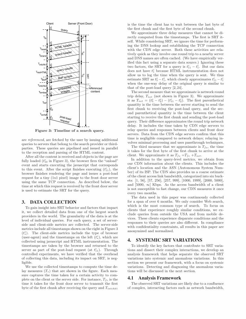
SRVW�ORDG�UHTXHVW

TXHU\

7KHDG

7EUDQG

7VF

7UHV+70/

7%R3

7HPEHG

7IV

657

7VFULSW

W�F

W�F

W�F

W�V

W�V

W�V

&OLHQW 6HUYHU��)URQW�'RRU�

7LQWFKN�

W��F

EUDQG�KHDGH

U

W�V

7LQWFKN�

UHIHUHQFHG�FRQWHQW

TXHU\�UHVXOWV

+70/�KHDGH

U

HPEHGGHG�

LPDJHV

%R3�VFULSWV

W��F

7UHI

7IF

7WF

W�V

W�F

W�F

W�F

W�F

W�F

W�F

Figure 3: Timeline of a search query.

are referenced, are fetched by the user by issuing additionalqueries to servers that belong to the search provider or third-parties. These queries are pipelined and issued in parallelto the reception and parsing of the HTML content.After all the content is received and objects in the page are

fully loaded (tc10 in Figure 3), the browser fires the “onload”event and starts executing the javascript that correspondsto this event. After the script finishes executing (tc11), thebrowser finishes rendering the page and issues a post-loadrequest for a tiny (1x1 pixel) image to the front door serverusing the same TCP connection. As described below, thetime at which this request is received by the front door serveris used to estimate the SRT for the query.

3. DATA COLLECTIONTo gain insight into SRT behavior and factors that impact

it, we collect detailed data from one of the largest searchproviders in the world. The granularity of the data is at thelevel of individual queries. For each query, a set of server-side and client-side metrics are collected. The server-sidemetrics include all timestamps shown on the right in Figure 3(ts∗). The client-side metrics include the type of browser(user-agent) and the timestamps on the left (tc∗), which arecollected using javascript and HTML instrumentation. Thetimestamps are taken by the browser and returned to theserver as part of the post-load request (at tc11). Throughcontrolled experiments, we have verified that the overheadof collecting this data, including its impact on SRT, is neg-ligible.We use the collected timestamps to compute the time de-

lay measures (T∗) that are shown in the figure. Each mea-sure captures the time taken for a certain activity to com-plete on the client or the server side. For instance, Tfc is thetime it takes for the front door server to transmit the firstbyte of the first chunk after receiving the query and Tintchk1

is the time the client has to wait between the last byte ofthe first chunk and the first byte of the second chunk.

We approximate three delay measures that cannot be di-rectly computed from the timestamps. The first is SRT it-self. While considering SRT, we ignore the time for perform-ing the DNS lookup and establishing the TCP connectionwith the CDN edge server. Both these activities are rela-tively quick as they involve one round trip to a nearby serverand DNS names are often cached. (We have empirically ver-ified this fact using a separate data source.) Ignoring thesetwo factors, the SRT for a query is tc11 − tc1. But our datadoes not have tc1 because HTML instrumentation does notallow us to log the time when the query is sent. We thusestimate SRT as ts5 − ts1, which closely approximates tc11 − tc1when the one-way delay of the original query is similar tothat of the post-load query [2, 24].

The second measure that we approximate is network roundtrip delay, Tnet (not shown in Figure 3). We approximateit as Tnet = (ts5 − ts2) − (tc11 − tc2). The first parentheticalquantity is the time between the server starting to send thefirst chunk to receiving the post-load query, and the sec-ond parenthetical quantity is the time between the clientstarting to receive the first chunk and sending the post-loadquery. Their difference approximates the round trip networkdelay. It includes the time taken by CDN edge servers torelay queries and responses between clients and front doorservers. Data from the CDN edge servers confirm that thistime is negligible compared to network delays; relaying in-volves minimal processing and uses passthrough techniques.

The third measure that we approximate is Tfs, the timeit takes for the first byte of the first chunk to arrive at theclient. We approximate it as Tfs =Tfc +Tnet.

In addition to the query-level metrics, we obtain fromour CDN information about the clients. This includes theclient’s location and the ASN (Autonomous System Num-ber) of its ISP. The CDN also provides us a coarse estimateof the client access link bandwidth, categorized into six buck-ets: [1, 56], [57, 256], [257, 999], [1000, 1999], [2000, 5000],and [5000, ∞] Kbps. As the access bandwidth of a clientis not susceptible to fast change, our CDN measures it onceevery two months.

The data used in this paper was continuously collectedfor a span of over 6 months. We only consider Web search,which is the most common type of search. To focus onclients that experience roughly similar conditions, we ex-clude queries from outside the USA and from mobile de-vices. These clients experience disparate conditions and theresponses to their queries are also different. In compliancewith confidentiality constraints, all results in this paper areanonymized and normalized.

4. SYSTEMIC SRT VARIATIONSTo identify the key factors that contribute to SRT varia-

tions and dissect their complex interactions, we develop ananalysis framework that helps separate the observed SRTvariations into systemic and anomalous variations. In thissection we present our framework, with a focus on systemicvariations. Detecting and diagnosing the anomalous varia-tions will be discussed in the next section.

4.1 Analysis FrameworkThe observed SRT variations are likely due to a confluence

of complex, interacting factors such as network bandwidth,

Measure Impact factorsTfs network, serverThead browser, networkTbrand browser, networkTintchk1 query, server

TresHTML browser, query, networkTBoP browser, query

Tintchk2 query, serverTembed query, networkTref browser, query, network

Tscript browser, queryTfc serverTsc query, serverTtc query, serverTnet network

Table 1: Factors that impact each measure.

end-to-end latency, server-side processing time, and browserspeed. To isolate and identify the key contributing factors,we start by decomposing the overall SRT into individualmeasures shown in the first column of Table 1. See Figure 3for what each measure represents. The relationship betweenindividual measures and underlying factors of interest (e.g.,network) is in general not one-to-one. As shown in Table 1,most measures are impacted by multiple factors, and eachfactor impacts multiple measures. A factor may also influ-ence different measures in different degrees (i.e., the effectsare unbalanced). These complex dependencies make it hardto tease out the factors that cause SRT variations; we can-not simply correlate SRT to measures that cleanly captureindividual factors. We describe below how we identify whichfactors cause most variation and quantify their impact.

4.1.1 Methodology

Let Y be a random, response variable that represents theobserved SRT, and let Xk, k = 1, 2, . . . , n, be a set of ran-dom, explanatory variables. Each Xk represents one of theconstituent measures in Table 1. We assume a linear modelM := Y = a0 +

∑k akXk + η, where η represents random

noise in measurements. This model is an approximationbecause the dependence between Y and Xk may not be lin-ear in practice. Further, because of dependencies betweenexplanatory variables, the model may not have a unique so-lution. But we find this simple model to be useful in analysisand we are careful to account for variable interaction whenusing the model. We use measurement data to learn a0 andak’s that best match the model M .Given this model, our analysis proceeds in three steps.

First, we separate the variance due to random noise in themeasurement from the the variance captured by the model.The latter is what we refer to as systemic variance. Second,given the systemic variance thus extracted, we quantify thecontribution of individual measures Xk, which in turn letsus identify the primary factors that cause SRT variation. Fi-nally, we investigate the contribution of each primary factorby controlling the other primary factors. In this subsection(§4.1), we described the first two steps, followed by their re-sults. Investigations that correspond to the final step are in§4.2–4.4.In the first two steps of our analysis, we apply ideas from

analysis of variance (ANOVA) [15]. The first step starts bycomputing the variance in the response variable, SST (Y ) =∑

i(yi−y)2, where yi is an individual (independent) observa-tion of the response variable and y is the mean value across

0

20

40

60

Exp

lain

ed

SS

(%

)

1st order

nth order

Tnet

TBoP

Tref

Tscript

TresHTML

Tsc

Ttc

Tfc

Thead

Figure 4: Analysis of variance results.

all observations. We then partition SST (Y ) into SSR(M,Y )and SSE(M,Y ), i.e., SST (Y ) = SSR(M,Y ) + SSE(M,Y ),where SSR(M,Y ) is the variance in Y explained by themodel M and SSE(M,Y ) is the variance that is not ex-plained by the model.1 Let yi = a0 +

∑k akxki, where

xki is an individual observation of the explanatory variableXk. Then SSR(M,Y ) =

∑i(yi − y)2, and SSE(M,Y ) =∑

i(yi − yi)2.

In the second step of our analysis, we partition the modelvariance SSR(M,Y ) into n components, each of which isattributable to an explanatory variable and helps quantifythe extent to which that variable explains SRT variance. Forthis purpose, we focus on two important metrics:

i) 1st order variance SSR(Mk, Y ): It quantifies the vari-ance explained by only one explanatory variableXk, as if theSRT depends on only one variable. That is, SSR(Mk, Y ) isthe model variance of the model Mk := Y = bk0 + bkXk + η.Formally, SSR(Mk, Y ) =

∑i(b

k0 + bkxki − y)2, where values

for bk0 and bk are learned from the measurement data.ii) n-th order variance SSR(M¬k, Y ): It quantifies the

left-over variance that is explained by Xk but cannot beexplained by the interactions of the other n − 1 variables.That is, SSR(M¬k, Y ) is the model variance of the modelM¬k := Y = ck0+

∑j 6=k c

kjXj+η. Formally, SSR(M¬k, Y ) =∑

i(ck0 +

∑j 6=k c

kjxji − y)2, where values for ck0 and ckj ’s are

learned from the measurement data.We apply the steps above on 1-hour averages of SRT and

the individual delay measures listed in Table 1. For com-putational efficiency and minimizing redundancy, we con-sider only those individual measures that have a noticeableimpact on SRT. Specifically, we exclude from our analysismeasures that either constitute a minuscule fraction of SRTor are highly correlated with another measure. The first cri-terion excludes Tintchk2 and Tembed because they representless than 1% of the SRT. The second excludes Tfs, Tintchk1,and Tbrand because they are highly correlated with, respec-tively, Tnet, Tsc, and TresHTML; the Pearson’s correlationcoefficients are 0.99, 0.79, 0.99. (High correlation betweenTfs and Tnet indicates that Tfs is largely determined by net-work latency, and the server-side processing time to generatethe first chunk (Tfc) has only a minute effect.)

4.1.2 Results: Primary factors

Figure 4 shows the amount of variation in SRT that isexplained by each of the 9 remaining measures. Focusingon the 1st order variance first, we see that the two mea-sures that explain the most variations, roughly 60% each,are Tnet and TBoP . Tnet is impacted by the network latencybetween the client and the (tier-1) server. TBoP is impacted

1In this notation, SS is short for sum of squares. The sub-scripts T , R, and E are short for total, regression, and error.

M T W Th F S Sut

1.26*t

Tn

et (

ms)

M T W Th F S Sub

1.25*b

BW

(K

bp

s)

Figure 5: Variation in network characteristics.

mainly by the browser speed and query type (e.g., resultspages with more images have more complicated bottom-of-page scripts). The next three measures explain roughlyequal amounts of variations, around 30% each. Of these,TresHTML and Tref are impacted by network latency andbandwidth since they involve downloading, respectively, ofthe results page and referenced content, by the query typesince size of the results page and referenced content dependon query, and by the browser’s speed of rendering the re-sults and referenced content. Tscript depends mainly on thebrowser’s speed of javascript execution.The measures that are impacted by the server processing

time, Tfc, Tsc, and Ttc, explain relatively small amount ofvariations in SRT. (Some of these measures are impactedby the query type as well.) Thus, all measures that explainsignificant SRT variations are impacted by network, query,and browser, but not by the server-side processing time.Interpreting these results requires some care. Our results

do not imply that server-side processing time is not an im-portant contributor to the total SRT. Server time could be abig fraction of SRT and yet not be responsible for significantsystemic variation because of its relative stability. This sta-bility could stem from techniques in the data center thatgenerate response within a configured deadline (e.g., 250ms) [6, 10]. Further, since we study average SRT across allqueries in an hour, our results also do not imply that serverprocessing time is stable at the level of individual queries.Various short-lived issues (e.g., OS-level scheduling) couldlead to high server delays for individual queries [13] and yetthose delays may not be a factor behind systemic variationsacross hours of the day.Next, looking at the n-th order variance, we see that most

variables explain only a small amount of variance that can-not be explained by other variables. This underscores thehigh degree of interaction among various variables. Tnet isthe only variable with notable n-th order variance.Though not shown in the figure, we also find that col-

lectively these measures capture almost all of the variancein SRT. The amount of SRT variations that cannot be ex-plained by them (i.e., SSE) is only 0.66%.In summary, we find that the systemic variations in SRT

stem primarily from network characteristics, query type, andbrowser speed; server-side processing time has a relativelysmall impact. That these three factors lead to systemic SRTvariations implies that they must be systemically varyingacross times of day and days of week. The following sectionsinvestigate how and why these three factors vary.

4.2 Variation in Network CharacteristicsWe begin by studying variation in network characteristics.

We show that it stems from changes in the relative fraction ofqueries that come from residential and enterprise networks.

Figure 5 shows the network characteristics observed acrossall of our clients. For a week-long period, it plots the hourlyaverage of network latency (Tnet) and the bandwidth (BW)reported by our CDN. All the graphs in this paper that showa week’s worth of data correspond to the same week; unlessthere is a weekday holiday, other weeks have similar behav-iors. We see the network characteristics do vary systemicallyover time. During off-peak hours, network latency increasesby as much as 20% and the bandwidth decreases by a simi-lar percentage. These systemic changes explain why networkcharacteristics is a key factor underlying SRT variations.

Now, the question is why network characteristics vary asshown. If anything, we would have expected the opposite:due to possible congestion during peak hours, network la-tency should have been higher during peak hours. As weexplain below, the variations we see are due to the variationsin the fraction of queries that come from residential networkswhich tend to have higher latencies and lower bandwidthscompared to enterprise networks.

We use a simple heuristic to classify a network as resi-dential or enterprise, based on the expectation that enter-prise networks send relatively few queries during weekends.For each of the 13,349 ASNs observed in our data, we com-pute the ratio of the number of queries they send duringthe weekend days (i.e., Saturday and Sunday) to the num-ber during weekdays. Across all ASNs, this ratio varies be-tween 0 and 10. For a conservative classification, we deemone-third of the ASNs with the lowest ratios as mainly-

enterprise and one-third of the ASNs with the highest ra-tios as mainly-residential. The middle third is deemed asmixed-or-unknown. The weekend-to-weekday query ratio ofall mainly-enterprise ASNs is lower than 0.0074. We do notexpect the ratio to be perfectly zero for many enterprises ifsome employees work on the weekends or connect their lap-tops through corporate VPNs (Virtual Private Networks).We manually verified the classification of many ASNs thatare deemed mainly-residential or mainly-enterprise, basedon their names. For instance, Microsoft (ASN 3598) is clas-sified as mainly-enterprise.2

With this classification in place, we can now explain thevariation in network characteristics. As shown in Figure 6,the mainly-residential ASNs send a greater proportion ofqueries during off-peak hours (left graph) and they havepoorer network characteristics (middle two graphs). Theirshare is 70% during peak hours but almost 100% during theoff-peak hours, and their network latency is 25% higher thanthat of mainly-enterprise ASNs.

The poorer network characteristics of mainly-residentialASNs translate, expectedly, to higher SRTs (right graph).On average, the SRT for these ASNs is 11.2% higher thanthat of mainly-enterprise ASNs. Due to the low traffic vol-ume from mainly-enterprise ASNs during off-peak hours, weonly plot their performance during weekday peak hours. Toillustrate this behavior without conflating with the impactof browser speed and query type on SRT, the graph is plot-

2We tried initially to use ASN names to classify ASNs butdropped that effort because of the names of many ASNs arehard to interpret.

M T W Th F S Su0

100

Fra

ctio

n o

f q

ue

rie

s (

%)

M T W Th F S Su

t

1.5*t

Tn

et (

ms)

M T W Th F S Sub

1.5*b

BW

(K

bp

s)

M T W Th F S Sut

1.57*t

SR

T (

ms)

mainly−ent mixed/unknown mainly−res

Figure 6: Comparing mainly-enterprise, mixed-or-unknown, and mainly-residential ASNs.

n 2+nt

3*t

Number of images

Tim

e (

ms)

Tref

Tscript

n 2+ns

3+s

Number of images

HT

ML

siz

e (

KB

)

(a) (b)

Figure 7: Image count vs. other measures of re-sponse page complexity.

ted using data that corresponds to only one type of browserand queries that generate similar response pages (specifi-cally, pages without images). Other browsers and querytypes show a similar effect.

4.3 Variation in Query TypeWe now investigate the variation in query type. The na-

ture of the query can impact SRT in two ways. First, itcan impact the time it takes the server to compute the re-sults. Second, because different queries have different re-sponse pages, it can impact the time it takes to download allcontent (which includes HTML and multimedia content) andfor the browser to load the page (which includes javascriptexecution and rendering). We showed earlier that server pro-cessing time is not a primary factor in SRT variations, anddetailed measurements based on different types of queriesconfirms that the variation in server processing time is small.Thus, variations in SRT due to query type must largely

stem from the diversity and variations in type of responsesgenerated. While most queries generate ten Web answers(HTML links), depending on the query, the response pagecan also contain other types of answers such as news, images,videos, and maps. These differences lead to high degree ofdiversity in response pages. The number of HTML bytes inthe response page varies by an order of magnitude across in-dividual queries, and the number of embedded or referencedimages vary by more than a factor of two. Consequently,different response pages take different times to download,parse, and render.Though researchers have recently proposed general mea-

sures of Web page complexity [11], we use a simple metricthat is specific to the domain of search. Because most non-Web answers contain images, we use the number of imageson the response page as a metric for page complexity. Itturns out that, as shown in Figure 7, this metric is correlatedwith other possible measures of page complexity such astime to download all referenced content (Tref in left graph),

time to load the page after all content has been downloaded(Tscript in left graph), and HTML size (right graph).

Figure 8 shows that the number of images in query re-sponses varies systematically across hours of day and daysof week. Further, Figure 9 shows that the SRT is higherfor queries with more images in their responses. The spreadin SRT values is about 30%. To factor out the impact ofnetwork and browser type, this figure is plotted for one typeof browser and mainly-residential ASNs. We obtain quali-tatively similar results for other browser and ASN types.

Taken together, the two effects—variation in query rich-ness and its impact on SRT—explain why the nature of thequeries is a primary factor behind SRT variations.

One interesting question is why query richness varies withtime. An in-depth look at the data reveals that richer queriestend to be leisure-oriented such as queries about celebrities,holiday events, and travel destinations. Users tend to issuemore of such queries during off-peak hours or when theyare at home. As shown in Figure 10, the number of imagescontained in the queries from mainly-residential ASNs arehigher than those from mainly-enterprise ASNs. Therefore,the shift of the “user intent” from peak to off-peak hours iswhat leads to variations in query richness.

4.4 Variation in Browser TypesWe now show that browsers are a primary factor behind

SRT variations because i) the relative mix of browsers ac-cessing the search service varies over time; and ii) differentbrowsers have different speeds.

There are eight types of browsers in our data that issue atleast 1% of the queries. Different major versions of the samebrowser (e.g., Internet Explorer 8 and 9) are considered dif-ferent types of browsers because they can have significantlydifferent rendering and script execution engines.

Figure 11 shows the variations of the fraction of queriesfor the two most popular browsers, Browser-X and Browser-Y. These two browsers account for 35% and 40% of the totalqueries, respectively. We see that the fraction of queries fromthese browsers varies substantially with time. Their relativepopularity swings by over 25%: Browser-X goes from gen-erating 15% more queries during peak hours to generating10% fewer queries. The relative popularity of other six ma-jor browser types varies as well. Two of them vary likeBrowser-X, i.e., they send a higher fraction of their queriesduring peak hours. The remaining four vary like Browser-Y.

In addition to generating different fractions of queries overtime, different browsers have disparate performance. As anindicator of browser performance, we use Tscript, which isnot impacted by the time it takes to download the page be-

M T W Th F S Sun

2.5+nN

um

be

r o

f im

ag

es

Figure 8: Variation in the imagecount in response pages.

n 1.6+nt

1.5*t

Number of images

SR

T (

ms)

Figure 9: SRT vs. image count inresponse pages.

M T W Th F S Sun

2+n

Num

ber

of

images

mainly−ent

mixed/unknown

mainly−res

Figure 10: Image count variationin different networks.

M T W Th F S Su

30

35

40

45

50

Pe

rce

nta

ge

(%

)

Browser−X Browser−Y

Figure 11: %-age of queries from the top twobrowsers.

M T W TH F S Su

t

3*t

Tscrip

t (m

s)

Browser−X Browser−Y

Figure 12: Tscript for the two major browsers.

cause it captures the time from downloading all content tofully loading the page. Figure 12 shows the performanceof the two popular browsers. On average, Browser-X isslower by a factor of 1.82. To minimize the impact fromnetwork and query type, we only plot it for queries whoseresponse pages do not contain images and come from mainly-residential ASNs; other types of queries and ASNs show asimilar behavior. As we can see from the figure, the twobrowsers have disparate performance. Controlled experi-ments on the same machine with different browsers confirmthat the differences in Tscript times that we see in the wildreflect real differences in browser performance, and not justdifferences in the capabilities of host machines.The combination of the two observations—variations in

the browser mix and the differences in browser speed—explainswhy browsers are a primary factor behind SRT variations.To understand why the mix of browsers varies with time,

we investigated where their users come from. Figure 13shows the fractions of queries coming from three differentcategories of networks for the two popular browsers. We seethat the vast majority of the Browser-Y’s queries come frommainly-residential networks. For Browser-X, however, thereis a significant shift (around 40%) during peak hours awayfrom mainly-residential networks. We speculate that thesetrends stem from the fact that Browser-X, at the time ofthis study, is more likely to be the standard browser that isadopted and supported officially by many enterprises. This

M T W Th F S Su0

50

100

Pe

rce

nta

ge

(%)

M T W Th F S Su0

50

100

Pe

rce

nta

ge

(%)

mainly−ent mixed/unknown mainly−res

Browser−X

Browser−Y

Figure 13: %-age of queries from diff. nets.

speculation is supported by the fact that Browser-X is anolder browser, while Browser-Y is newer; many enterprisesin the USA do not immediately upgrade to newer browsersas they must first test compatibility of the new browser withtheir internal services (called line-of-business applications).On the other hand, residential machines in the USA arelikely upgraded sooner due to automatic updates. Thus, asthe users of the search service move from work to home, theservice sees a move from Browser-X to Browser-Y.

Observe that the impact of browsers on SRT is the oppo-site of the impact of network and query type. During off-peak hours, a greater fraction of queries come from Browser-Y, which has better performance. This should have a pos-itive impact on SRT during off-peak hours. But the nega-tive impact on SRT due to variations in network and querytype dominates, and we see higher SRTs as the net effect.Without the corrective effect of browsers, the SRTs duringoff-peak hours would have been even higher.

5. ANOMALOUS SRT VARIATIONSIn addition to systemic variations that we study above,

SRT also experiences irregular variations. These variations,which we call anomalies, stem from events such as failures inthe network or data center, congestion, and attacks on thesearch infrastructure. For a good user experience, anomaliesmust be detected and resolved quickly. However, operatorsinform us that it frequently takes them several days beforethey even detect that the SRT is anomalous, as the systemicvariations often hide the real anomalies. Once detected, di-agnosing the root cause of an anomaly is also challenging asit can lie in any part of the infrastructure.

We develop a technique to assist the operators in quicklydetecting and diagnosing SRT anomalies. Below, we firstdescribe how it detects anomalies and then how it localizestheir root causes. We have implemented our technique in atool that has been deployed on the real system.

5.1 Detecting AnomaliesThe main challenge in accurately detecting SRT anomalies

is that they co-exist with systemic variations due to otherfactors, including the weekly, daily and hourly fluctuations,and the long-term evolution of SRT. As we show later, dueto these variations, common anomaly and outlier detectionmethods both fail to detect many anomalies and flag eventsthat are not anomalies.

5.1.1 Methodology

We use an approach based on time series decomposition [26],which we call WoW (week-over-week) analysis. The basicidea is to view SRT as a composition of three components:i) the long-term trend; ii) the seasonality or periodic behav-ior; and iii) fast variations or noise.Consider the SRT time series, where SRTt is the average

over the t-th hour. The long-term trend component, denotedby L, of this series can be computed as a centered movingaverage with the window size set to T :

Lt =1

T + 1

T/2∑

i=−T/2

SRTt+i (1)

T should be greater than or equal to the maximum period-icity in the data. We use T=168 hours (1 week).Let Yt=SRTt–Lt be the time series after removing the

long-term trend. Then, the seasonal component, S, can becomputed as seasonal moving average:

St =1

M + 1

M∑

i=0

Yt−iT ,M = ⌊t/T ⌋ (2)

What remains now is the noise component, N, which canbe computed by removing the long-term trend and season-ality components:

Nt = SRTt − Lt − St (3)

By definition, this component is neither part of the longterm trend nor a periodic event. It captures the irregularitythat cannot be explained by the other two factors.We deem as anomalous time instances where the noise is

abnormally high. To infer high abnormality, we assume thatnoise follows a Gaussian distribution based on the centrallimit theorem [1]. However, due to the diurnal patterns andthe day of week effect, the distribution parameters can differfor different times of week.Thus, based on historical data, we learn 168 Gaussian

models, one for each hour of the week. We flag as anomalousvalues outside the 95th percentile of the distribution (i.e.,±1.96). This threshold is commonly used in many statisticalareas [25] and we find that it works well in our setting too.Thus, we deem that the SRT at time t is anomalous if:

|Nt − µt|

σt

> 1.96 (4)

where µt and σt are the mean and standard deviation of theGaussian distribution built from all data collected at thesame hours as t within a week.The quantity on the left in Eq. 4 is the severity of the

anomaly, and we report it in the notifications that are gen-erated for the operators. It captures the extent to whichcurrent SRT has deviated from expectation. Larger valuesindicate more serious anomalies.

M5 M6 M7 M8t

1.17*t

Tre

nd

(ms)

M5 M6 M7 M8

−50

50

Se

aso

na

lity

(ms)

M5 M6 M7 M8

−1.96

1.96

No

rma

lize

dN

ois

e

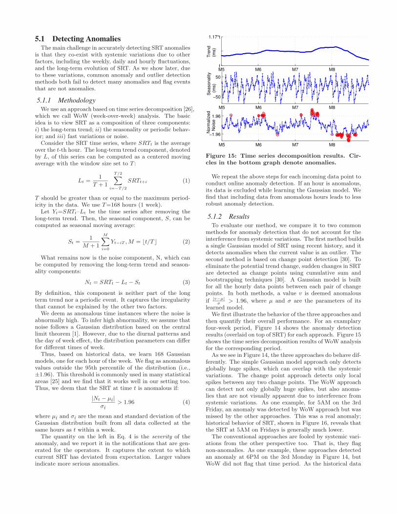
Figure 15: Time series decomposition results. Cir-cles in the bottom graph denote anomalies.

We repeat the above steps for each incoming data point toconduct online anomaly detection. If an hour is anomalous,its data is excluded while learning the Gaussian model. Wefind that including data from anomalous hours leads to lessrobust anomaly detection.

5.1.2 Results

To evaluate our method, we compare it to two commonmethods for anomaly detection that do not account for theinterference from systemic variations. The first method buildsa single Gaussian model of SRT using recent history, and itdetects anomalies when the current value is an outlier. Thesecond method is based on change point detection [30]. Toeliminate the potential trend change, sudden changes in SRTare detected as change points using cumulative sum andbootstrapping techniques [30]. A Gaussian model is builtfor all the hourly data points between each pair of changepoints. In both methods, a value v is deemed anomalous

if |v−µ|σ

> 1.96, where µ and σ are the parameters of itslearned model.

We first illustrate the behavior of the three approaches andthen quantify their overall performance. For an examplaryfour-week period, Figure 14 shows the anomaly detectionresults (overlaid on top of SRT) for each approach. Figure 15shows the time series decomposition results of WoW analysisfor the corresponding period.

As we see in Figure 14, the three approaches do behave dif-ferently. The simple Gaussian model approach only detectsglobally huge spikes, which can overlap with the systemicvariations. The change point approach detects only localspikes between any two change points. The WoW approachcan detect not only globally huge spikes, but also anoma-lies that are not visually apparent due to interference fromsystemic variations. As one example, for 5AM on the 3rdFriday, an anomaly was detected by WoW approach but wasmissed by the other approaches. This was a real anomaly;historical behavior of SRT, shown in Figure 16, reveals thatthe SRT at 5AM on Fridays is generally much lower.

The conventional approaches are fooled by systemic vari-ations from the other perspective too. That is, they flagnon-anomalies. As one example, these approaches detectedan anomaly at 6PM on the 3rd Monday in Figure 14, butWoW did not flag that time period. As the historical data

M5 M6 M7 M8

t

1.17*t

SR

T (

ms)

data Gaussian Change point WoW

6PM3rd Monday

5AM3rd Friday

Figure 14: Comparing anomaly detection results for three different techniques.

M1 M2 M3 M4 M5 M6 M7

t

1.17*t

SR

T (

ms)

data 6PM, Mondays 5AM, Fridays

missed realanomaly

flaggednon−anomaly

Figure 16: Historical behavior for the anomalies flagged or missed by Gaussian and change point techniques.

in Figure 16 displays, this time period does not have signif-icantly degraded SRT compared to 6PM on past Mondays.We now perform a more systematic evaluation. The per-

formance of anomaly detection can be quantified using falsenegative and positive rates. False negatives are cases inwhich a real anomaly is missed, and false positives are casesin which a non-anomaly is flagged. The results below arebased on five months of data.False negatives: Quantifying the false negative rate re-quires as a reference a complete list of all anomalies in thesystem. However, such a list is rarely available for a com-plex, real system. We use instead the ticket database thatis maintained by the search provider. The anomalies doc-umented in this database have been manually detected bythe operators based on visual inspection of the data or usercomplaints, or they have been flagged by an existing tool(which does not account for SRT variations) and later veri-fied manually.We find that 90%, 65%, and 60% of all the anomalies

present in this database are identified by WoW, Gaussian,and change point approaches. That is, while WoW missed10% of the anomalies, the other approaches miss 3-4 timesas many.Comparing the ticket database and our tool, we find that

the anomalies in the database tend to have high severityvalues (> 2.5, or outside the 99th percentile of the Gaus-sian model). This implies that with the current practice,operators could detect only highly anomalous events. Fur-ther, our tool flags many anomalies that are not in the ticketdatabase. If these anomalies are not false positives, whichwe study next, they represent anomalies that the currentpractice misses.False positives: Estimating the false positive rate of ananomaly detection tool is challenging. Investigating an anomalycan take a huge amount of effort and thus operators do notinvestigate each anomaly. For instance, short-lived anoma-lies that disappear before an operator has had a chance toinvestigate are not investigated. (However, operators still

0.5 1 1.5 2 2.5 3 3.5 4 4.5 50

0.2

0.4

0.6

0.8

1

Largest severity in measures

CD

F

Change Point

Gaussian

WoW

Figure 17: Distribution of largest severity across allmeasures.

want to detect and log all anomalies; this record helps quan-tify service reliability and determine if some components failrepeatedly.) Thus, we cannot be sure if a certain anomalythat was flagged by our tool but not investigated is a trueor a false positive.

To estimate the false positive rate, we emulate the methodused by the operators as a first step towards investigatingan anomaly. The operators observe the behavior of other,fine-grained measures (e.g., Tnet) during the anomaly pe-riod. If one or more of those measures is anomalous as well,the anomaly is deemed as likely real and further investiga-tion is conducted. If none of those measures is anomalous,the anomaly is deemed as false. The assumption is that ifthe anomalous behavior in SRT correlates to anomalous be-havior in at least one of the fine-grained measures, then wecan be confident that this is a real anomaly.

Thus, we apply the same WoW technique to the 14 fine-grained measures (§4) and compute the largest severity valueacross all measures. Figure 17 shows the distribution of thelargest severity value as an SRT anomaly is detected usingthree different techniques. We consider an SRT anomalyto be a false positive, if the largest severity value does notindicate an anomaly, that is, it is under 1.96. Based onthis criteria, we see that the false positive rate of WoW is

Ttc

Tsc

Tfc

Tintchk2

Tintchk1

Tnet

Tfs

Tscript

Tref

Thead

TBoP

Tbrand

TresHTML

Tembed

Tem

bed

Tre

sH

TM

L

Tbra

nd

TB

oP

Thead

Tre

f

Tscript

Tfs

Tnet

Tin

tchk1

Tin

tchk2

Tfc

Tsc

Ttc

5 %

10%

15%

20%

25%

30%

35%

40%

Figure 18: %-age of anomalies for pairs of measures.

7%, while that of Gaussian (17%) and change point (19%)approaches is at least twice as much.

5.2 Diagnosing AnomaliesIn addition to detecting anomalies, our tool helps oper-

ators diagnose those anomalies, by identifying at a coarse-level the most likely source of the problem. For our purposes,possible sources are client behavior, the data center, and thenetwork between the clients and the data center (which in-cludes the CDN servers). Client behaviors can be a sourceof anomalies due to attacks (e.g., bots generating a lot ofqueries), among other possibilities.The inference of our tool is then combined with other

lower-level measures (e.g., output of tools that monitor net-work or server health and utilization) to localize the rootcause at a finer granularity. These low-level measures areby themselves insufficient for root cause localization as theyare noisy and their impact on SRT is otherwise unclear [9].

5.2.1 Methodology

The anomaly diagnosis functionality of our tool is invokedwhenever an SRT anomaly is detected. Its starting pointsare the time series of the 14 measures that we used to studysystemic SRT variations.We face two main challenges. First, due to complex inter-

actions among different measures, simply using the anomalyseverity value of individual time series does not suffice. Forexample, when an anomaly happens in the network, bothTresHTML and Tnet can be anomalous. Second, during anoma-lies, the relationships among the different measures may varyfrom the normal case. For example, under normal circum-stances, Tfs (which is Tnet + Tfc) and Tnet are highly cor-related usually, but if Tfc is anomalous due to a failure inthe data center, this correlation disappears.Thus, a better understanding of the relationships among

the various measures during SRT anomalies is important. Toobtain insight into these relationships, we investigate how of-ten two measures are simultaneously anomalous during SRTanomalies. Figure 18 shows the percentage of SRT anoma-lies in which a pair of measures, specified on the x- andy-axis, appear as anomalies at the same time. The diagonalvalues are the percentage of SRT anomalies when the mea-sures, specified on the x (or y)-axis, appear as an anomalyby themselves. The graph is symmetric along the diagonal.We make the following observations from this figure. First,

focusing on Tnet, a pure network-side measure, we see thatTfs is almost always anomalous along with it. The server-side measures (Tfc, Tsc, Ttc) and client-side measures that

M T W Th F S Sut

3*t

SR

T (

ms)

M T W Th F S Sut

2.5*t

SR

T (

ms)

M T W Th F S Sut

2.5*t

SR

T (

ms)

t

2.1*t

Tsc (

ms)

t

1.75*t

Tnet (

ms)

n

1.5+n

# im

ag

es

(a)

(b)

(c)

Figure 19: Example anomalies.

are highly dependent on the server behavior (Tintchk1 andTintchk2) are rarely anomalous in conjunction with Tnet.Other browser-side measures are sometimes anomalous inconjunction with Tnet. Second, let us focus on pure server-side measures (Tfc, Tsc, Ttc). They appear anomalous mostlyon their own, except for i) Tintchk1, which is a browserside measure that is highly dependent on server-side la-tency; and ii) Tintchk2 and Tembed, which we can ignoreas they contribute less than 1% of the total SRT. Third,the anomalies in browser-side measures (TresHTML, Tbrand,TBoP , Thead, Tref , and Tscript) are weakly correlated withserver- and network-side measures, indicating their anoma-lies likely stem from client issues.

Based on the observations above, to diagnose anomalies,we first divide the measures into three classes: Network(Tnet and Tfs), Server (Tfc, Tsc, Ttc), or Client (TresHTML,Tbrand, TBoP , Thead, Tref , and Tscript). If only one class ofmeasures is anomalous, then we deem the problem likely liesin the corresponding class. We saw above that, frequently,only one class is anomalous when SRT is anomalous.

If measures in more than one class are anomalous, weuse the following decision logic to determine the likely rootcause (or prioritize the investigation). First, if any Servermeasures are anomalous, we deem that the anomaly is inthe data center. This heuristic is based on the second obser-vation above and the fact that the server-side measures arecollected using a separate instrumentation (not Javascript),which is not supposed to be affected by the impact from thenetwork or client-side behaviors.

Second, if Tnet is anomalous, but not any Server mea-sure, then we consider it as an anomaly associated with thenetwork. The underlying rationale is that because of theway we compute Tnet (§3), it is not intimately dependenton client behavior. This is also supported by the first obser-vation above. Finally, we consider that the remaining casesare due to client behaviors (e.g., bot attacks).

5.2.2 Results

Using the diagnosis method described above, we deter-mine the root cause for each of the detected anomalies andcompare them with what is inferred and logged by the oper-ators in the ticket database. We find that our results are per-fectly consistent with the ticket database for those anomaliesthat are common to both methods.

Figure 19 shows three example anomalies. For each, SRTuses (blue) crosses and the left y-axis, another metric of in-terest uses (green) dots and the right y-axis, and the anoma-lous periods are marked using (red) circles. In the case ofFigure 19(a), our tool diagnosed that the backend data cen-ter was the likely culprit because Tsc and SRT were anoma-lous at the same time. Figure 19(b) was diagnosed as a net-work failure (due to a re-configuration of the routing weightsbetween the CDN edge servers and the backend data cen-ters) using our tool, as it was accompanied by anomalousTnet. On the other hand, the culprit in Figure 19(c) wasthe change of query richness during a major holiday event.Although no action needs to be taken to resolve this perfor-mance degradation, our tool helped the operators eliminatethe possibilities of failures in the data centers or the network.Across all SRT anomalies that our tool detected, we find

that the fractions of the anomalies that were attributed tothe wide-area network, data center, and client behaviors are37%, 27%, and 36%, respectively. That the culprits are al-most evenly distributed (with the data center being slightlylower), means that there is no silver bullet to significantlyreduce the bulk of the SRT anomalies. The provider mustwork on reducing the impact of failures and unexpected be-haviors on all three fronts. Perhaps the most surprisingaspect is that client behaviors account for a third of theanomalies. Most of these are attacks on search infrastruc-ture, but some are also caused by sudden changes in queryrichness (e.g., following a major newsworthy event).

6. IMPLICATIONS AND DISCUSSIONOur work has several implications for managing, under-

standing, and diagnosing the performance of large-scale Webservices. We discuss a few of them in this section.

Performance management: A key goal of many Webservices is to provide consistently good performance to theirusers. Work on this front has mainly focused on consis-tent request processing delays within the data center [6,10].Our findings, however, show that focusing on server pro-cessing time alone is insufficient and much of the variationin users’ performance stems from factors such as networkpaths, browsers, and query types. While these factors arenot under direct control of the service provider, there areways in which their impact can be minimized.For network paths, the service provider can send simpler

pages for queries that come from clients behind slow last milelinks. Using a data source that is different from the one usedin this paper we find that the middle mile between the datacenter and the edge exhibits significant performance varia-tions as well. This variations can be controlled through ded-icated capacity between these points. One major providerappears headed in that direction already [23].To ensure consistently fast SRTs across browsers, the providers

can customize the responses and scripts to account for thestrengths and weaknesses of individual browsers. Our dataindicates that customization for the top three or four browserswould cover the vast majority of the queries.To ensure fast SRTs for rich queries, the CDN edge servers

can help reduce the burden on the user’s end (browser) bysimplifying dynamically the layout of the page and pre-processing some of the scripts. They can also cache moreof the CSS, images, and javascript. Caching on the edge isnot used heavily today because bits of the response pages

are personalized. Small amount of computational capabili-ties on the edge servers (for generating personalized portionsof the page) and a different layout of the response page canimprove the amount of the content that users can fetch fromthe edge servers.

Performance monitoring: Our work highlights the dif-ficulty of reasoning about service performance when it ismeasured across all users because such a measure is taintedby systemic changes in behaviors and characteristics of userpopulation. This holds not only for search but for otherWeb services as well. For instance, Zander et al. [34] ob-served different fraction of users with IPv6 capabilities onweekends vs. weekdays for many services. (They could notfully explain this variation. Our results confirm their sus-picion that it stems from residential and enterprise usershaving different characteristics.)

To provide greater insight into service performance, weare developing techniques to partition requests into equiv-alence classes that account for expected performance dif-ferences across network paths, browsers, and query types.This would enable the operators to better monitor and un-derstand performance variation within a class, which other-wise gets masked by changes in the fractions of queries inindividual classes.

Performance diagnosis: Another difficulty highlighted byour work is that of detecting and diagnosing performanceanomalies. Past research has argued for using end-to-endperformance metrics, rather than relying on low-level met-rics such as server processing time, CPU or network utiliza-tion, because the anomalies in low-level measures may ormay not cause anomalies in user experience [9,20]. But ourwork shows that using such measures is challenging due tosystemic variations. Prior work has looked at systems withroughly stationary response time characteristics because of alack of significant diversity in query types, browsers, and net-work paths, as may be the case in enterprise networks [9,20].But in the Web services context, effective diagnosis of re-sponse time requires factoring out systemic variations andappropriately combining high- and low-level metrics.

7. RELATEDWORKOur work builds upon much prior work on the perfor-

mance of Web services. One thread of work takes a client-side perspective to monitor the performance that a clientexperiences at various Web sites or to uncover factors thatimpact Web page load times. For example, WProf [32] andWebPagetest [4] are tools to measure the performance toany Web site and provide a timeline of relevant events thatoccur while the page is being loaded; and Butkietz et al. [11]examines the impact of page structure and server locationof various Web sites on a client’s performance. In contrast,our work takes a provider-side perspective, to uncover fac-tors that impact the performance delivered by a Web serviceto all its active clients.

Another thread of work focuses on improving differentaspects of Web services such as request processing, pagedesign, and content delivery. For example, several worksseek to make request processing predictable in a data cen-ter [7,33]; tools exist to help developers follow the best prac-tices for site layout and design [3, 5]; and many researchershave studied several facets of CDN design such as placement

and TCP behavior of edge servers [8, 12, 17, 19, 31] and pro-posed enhancements such as better redirection and caching,and hybrid CDNs [14,16,18,21,28]. In contrast to this bodyof work, we take an end-to-end view, which includes all rele-vant aspects, of the performance of a Web service. Further,instead of focusing on specific design enhancements, we seekto explain and diagnose performance variations given thedesign of a modern, large-scale service.

8. CONCLUSIONSOur work addresses the challenges in understanding and

diagnosing the performance of large-scale, Web services. Weshowed that the response time for a large service varieswidely and, surprisingly, increases during off-peak hours whenthe query load is lower. We developed an analysis frame-work that reveals that this variation stems from systemicshifts in user characteristics—the source networks, the na-ture of queries, and the browsers used. In contrast, serverprocessing times are relatively stable. We also developedand deployed a technique that detects and diagnoses serviceperformance anomalies by factoring out the impact of suchsystemic variations. We found that our technique detectedthree times more anomalies than conventional methods thatdo not account for systemic variations.

Acknowledgments

We thank Cheng Huang, Ritchie Hughes, Mujtaba Kham-batti, Venkat Narayanan, Aditya Telidevara, for feedbackin the initial stages of the project. We also thank AdityaAkella, Meg-Walraed Sullivan, the SIGCOMM reviewers,and our shepherd, Walter Willinger, for feedback on earlierdrafts of this paper.

9. REFERENCES[1] Central limit theorem. http://en.wikipedia.org/wiki/

Central_limit_theorem.[2] Measure page load time. https://developers.google.com/

speed/docs/pss/LatencyMeasure.[3] Pagespeed tools family. https://developers.google.com/

speed/pagespeed/.[4] WebPageTest - website performance and optimization test.

http://www.webpagetest.org/.[5] Yslow. http://yslow.org/.[6] T. Abdelzaher, K. Shin, and N. Bhatti. Performance

guarantees for Web server end-systems: Acontrol-theoretical approach. IEEE Transactions onParallel and Distributed Systems, 2002.

[7] E. Agichtein, E. Brill, S. Dumais, and R. Ragno. Learninguser interaction models for predicting Web search resultpreferences. In ACM SIGIR, 2006.

[8] M. Al-Fares, K. Elmeleegy, B. Reed, and I. Gashinsky.Overclocking the Yahoo! CDN for faster Web page loads.In IMC, 2011.

[9] P. Bahl, R. Chandra, A. Greenberg, S. Kandula, D. Maltz,and M. Zhang. Towards highly reliable enterprise networkservices via inference of multi-level dependencies. In ACMSIGCOMM, 2007.

[10] L. Barroso, J. Dean, and U. Holzle. Web search for aplanet: The Google cluster architecture. IEEE Micro, 2003.

[11] M. Butkiewicz, H. Madhyastha, and V. Sekar.Understanding website complexity: Measurements, metrics,and implications. In IMC, 2011.

[12] Y. Chen, S. Jain, V. Adhikari, and Z. Zhang.Characterizing roles of front-end servers in end-to-endperformance of dynamic content distribution. In IMC, 2011.

[13] J. Dean. Achieving rapid response times in large onlineservices. In Berkeley AMPLab Cloud Seminar, 2012.

[14] M. Freedman, E. Freudenthal, and D. Mazieres.Democratizing content publication with coral. In USENIXNSDI, 2004.

[15] A. Gelman. Analysis of variance, 2005. http://www.stat.columbia.edu/~gelman/research/unpublished/econanova.pdf.

[16] C. Gkantsidis and P. Rodriguez. Network coding for largescale content distribution. In IEEE INFOCOM, 2005.

[17] C. Huang, A. Wang, J. Li, and K. Ross. Measuring andevaluating large-scale cdns. In IMC, 2008.

[18] H. Jiang, J. Li, Z. Li, and X. Bai. Performance evaluation ofcontent distribution in hybrid CDN-P2P network. In IEEEFuture Generation Communication and Networking, 2008.

[19] K. Johnson, J. Carr, M. Day, and M. Kaashoek. Themeasured performance of content distribution networks.Elsevier, 2001.

[20] S. Kandula, R. Mahajan, P. Verkaik, S. Agarwal,J. Padhye, and P. Bahl. Detailed diagnosis in enterprisenetworks. In ACM SIGCOMM, 2009.

[21] J. Kangasharju, K. Ross, and J. Roberts. Performanceevaluation of redirection schemes in content distributionnetworks. Elsevier, 2001.

[22] R. Kohavi, R. M. Henne, and D. Sommerfield. Practicalguide to controlled experiments on the Web: Listen to yourcustomers not to the HiPPO. In SIGKDD, 2007.

[23] R. Krishnan, H. Madhyastha, S. Srinivasan, S. Jain,A. Krishnamurthy, T. Anderson, and J. Gao. Movingbeyond end-to-end path information to optimize CDNperformance. In IMC, 2009.

[24] A. Pinto. How to measure page load time with googleanalytics. http://www.yottaa.com/blog/bid/215491/How-to-Measure-Page-Load-Time-With-Google-Analytics.

[25] D. G. Rees. Foundations of statistics, volume 214.Chapman & Hall, 1987.

[26] M. Roughan, A. Greenberg, C. Kalmanek, M. Rumsewicz,J. Yates, and Y. Zhang. Experience in measuring backbonetraffic variability: Models, metrics, measurements andmeaning. In ACM IMW, 2002.

[27] A. Singhal and M. Cutts. Official Google webmaster centralblog: Using site speed in Web search ranking, 2009.http://googlewebmastercentral.blogspot.com/2010/04/using-site-speed-in-web-search-ranking.html.

[28] Y. Song, V. Ramasubramanian, and E. Sirer. Optimalresource utilization in content distribution networks.Technical Report TR2005-2004, Cornell University, 2005.

[29] S. Stefanov. Progressive rendering via multiple flushes.http://www.phpied.com/progressive-rendering-via-multiple-flushes/.

[30] W. Taylor. Change-point analysis: a powerful new tool fordetecting changes, 2000. http://www.variation.com/cpa/tech/changepoint.html.

[31] S. Triukose, Z. Wen, and M. Rabinovich. Measuring acommercial content delivery network. In ACM WWW,2011.

[32] X. S. Wang, A. Balasubramanian, A. Krishnamurthy, andD. Wetherall. Demystify page load performance withWProf. In USENIX NSDI, 2013.

[33] R. White and S. Dumais. Characterizing and predictingsearch engine switching behavior. In ACM conference onInformation and knowledge management, 2009.

[34] S. Zander, L. Andrew, G. Armitage, G. Huston, andG. Michaelson. Mitigating sampling error when measuringInternet client IPv6 capabilities. In IMC, 2012.